On Deep Learning Classification of Digitally Modulated Signals Using Raw I/Q Data

Abstract

The paper considers the problem of deep-learning-based classification of digitally modulated signals using I/Q data and studies the generalization ability of a trained neural network (NN) to correctly classify digitally modulated signals it has been trained to recognize when the training and testing datasets are distinct. Specifically, we consider both a residual network (RN) and a convolutional neural network (CNN) and use them in conjunction with two different datasets that contain similar classes of digitally modulated signals but that have been generated independently using different means, with one dataset used for training and the other one for testing.

I Introduction

Identifying a specific digital modulation scheme without specific knowledge about its parameters and/or without prior information on the transmitted data can be accomplished using likelihood-based approaches [1, 2] or cyclostationary signal processing (CSP) [3]. Recently, deep learning (DL) approaches to classifying digitally modulated signals have also been proposed, such as those in [4, 5], which use the raw I/Q signal components for training and signal recognition/classification, or the alternative approaches in [6, 7, 8, 9, 10], in which the amplitude/phase or frequency domain representations are used.

DL-based approaches implement neural networks (NNs) and rely on their extensive training to make the distinction among different classes of digitally modulated signals. Usually, the available data set is partitioned into subsets that are used for training/validation and testing, respectively, and it is not known in general how well NNs trained on a specific dataset respond to similar signals that are generated differently than those in the dataset used for training and validation. However, the problem of the dataset shift, also referred to as out-of-distribution generalization [11], is an important problem in machine-learning-based approaches, which implies that the training and testing data sets are distinct, and that data from the testing environment is not used for training the classifier. This problem motivates the work presented in this paper, which studies the performance of DL-based classification of digitally modulated signals when the training and testing data are taken from distinct data sets.

Specifically, the paper considers the DL-based approach to modulation classification discussed in [5, 4], which uses raw I/Q signal data to train NNs for use in classifying digitally modulated signals. To assess the generalizability of I/Q-trained NNs and evaluate how well they perform on classifying digitally modulated signals from datasets they were not trained on, we implement NNs with architectures similar to those in [4] training them with signals from one data set and evaluating their classification performance using signals in the other data set. The two data sets used are publicly available:

• DataSet1 was generated for use in [4] and can be downloaded from DeepSig Inc.’s website [12].

• DataSet2 was independently generated and is available on the CSP Blog [13].

The paper is organized as follows: Section II describes the NNs implemented for classification of digitally modulated signals, followed by presentation of the two data sets used for training and testing in Section III. Section IV discusses NN training details and presents numerical results showing the classification performance of the two NNs, with a focus on generalization, when training and testing are performed using signals from different data sets. The paper is concluded with final remarks in Section V.

II Neural Network Models for Digital Modulation Classification

DL NNs consist of multiple interconnected layers of neuron units and include an input layer, which takes the available data for processing, several hidden layers that provide various levels of abstractions of the input data, and an output layer, which determines the final classification of the input data [14]. The hidden layers of a NN include:

• Convolutional layers, may be followed by batch normalization to increase regularization and avoid overfitting.

• Fully connected layers that may be preceded by dropout layers.

• Nonlinear layers, with the two common types of nonlinearities employed being the rectified linear unit (ReLU) and the scaled exponential linear unit (SELU).

• Pooling layers that use average or maximum pooling to provide invariance to local translation.

• A final softmax layer that establishes the conditional probabilities for input data classification by determining the output unit activation function for multi-class classification problems.

TABLE I: Residual Neural Network Layout

Layer	Output Dimensions
Input	$2\times 1024$
Residual Stack	$32\times 512$
Residual Stack	$32\times 256$
Residual Stack	$32\times 128$
Residual Stack	$32\times 64$
Residual Stack	$32\times 32$
Residual Stack	$32\times 16$
Drop($50\%$)/FC/SELU	$128$
Drop($50\%$)/FC/SELU	$128$
Drop($50\%$)/FC/SoftMax	# Classes

TABLE II: Residual Stack Layout

Layer	Output Dimensions
Input	$X\times Y$
$1\times 1$ Conv	$32\times Y$
Batch Normalization	$32\times Y$
ReLU	$32\times Y$
Residual Unit	$32\times Y$
Residual Unit	$32\times Y$
Maximum Pooling	$32\times Y/2$

TABLE III: Residual Unit Layout

Layer	Output Dimensions
Input	$X\times Y$
Conv	$32\times Y$
Batch Normalization	$32\times Y$
ReLU_1	$32\times Y$
Conv	$32\times Y$
Batch Normalization	$32\times Y$
ReLU_2	$32\times Y$
Addition(Input, ReLU_2)	$32\times Y$

TABLE IV: Convolutional Neural Network Layout

Layer	Output Dimensions
Input	$2\times 1024$
Conv	$16\times 1024$
Batch Normalization	$16\times 1024$
ReLU	$16\times 1024$
Maximum Pooling	$16\times 512$
Conv	$24\times 512$
Batch Normalization	$24\times 512$
ReLU	$24\times 512$
Maximum Pooling	$24\times 256$
Conv	$32\times 256$
Batch Normalization	$32\times 256$
ReLU	$32\times 256$
Maximum Pooling	$32\times 128$
Conv	$48\times 128$
Batch Normalization	$48\times 128$
ReLU	$48\times 128$
Maximum Pooling	$48\times 64$
Conv	$64\times 64$
Batch Normalization	$64\times 64$
ReLU	$64\times 64$
Maximum Pooling	$64\times 32$
Conv	$96\times 32$
Batch Normalization	$96\times 32$
ReLU	$96\times 32$
Average Pooling	$96$
Drop($0\%$)/FC/SoftMax	# Classes

We note that commonly used types of NNs in DL include CNNs and RNs, with the latter including bypass connections between layers that enable features to operate at multiple scales and depths throughout the NN [14].

The study on DL-based classification of digitally modulated signals presented in this paper aims at assessing the generalization ability of trained NNs and demonstrating the need for more robust testing of NNs trained to recognize digital modulation schemes. In this direction, we consider both an RN with the layout specified in Tables I–III, and a CNN with the layout specified in Table IV. For both types of NNs (RN and CNN) the convolutional layers use a filter size of $23$ as increasing the filter size increases the computational cost with no performance gain, while decreasing it lowered performance.

The NN structures outlined in Tables I – IV are similar to those in [4], and that the novelty of this work consists in the use of two distinct datasets for training and testing, respectively, which will allow us to evaluate if the NNs are able to generalize and continue to distinguish the classes of digitally modulated signals for which they have been trained when tested on signals that are generated differently than the signals in the training dataset.

III Datasets for NN Training and Testing the Classification of Digitally Modulated Signals

The DL NNs used for classification of digitally modulated signals with the structure outlined in Section II are trained and tested using digitally modulated signals in two distinct datasets that are publicly available for general use, which are referred to as DataSet1 [12] and DataSet2 [13], respectively. These datasets contain collections of the I/Q data corresponding to signals generated using common digital modulation schemes that include BPSK, QPSK, 8-PSK, 16-QAM, 64-QAM, and 256-QAM, with different signal-to-noise ratios (SNRs). Brief details on the signal generation methods are also provided in the descriptions of the two datasets, and we note that the signals include overlapping excess bandwidths and the use of square-root raised-cosine (SRRC) pulse shaping with similar roll-off parameters.

According to [4], DataSet1 includes both simulated signals and signals captured over-the-air, with $24$ different modulation types and $26$ distinct SNR values for each modulation type, ranging from $-20$ dB to $30$ dB in $2$ dB increments. For each modulation type and SNR value combination, there are $4,096$ signals included in the dataset, with $1,024$ I/Q samples for each signal, and the total number of signals in DataSet1 is $2,555,904$.

DataSet2 [13] contains only simulated signals corresponding to $8$ different digital modulation types with SNRs varying between $0$ dB and $13$ dB. The dataset includes a total of $112,000$ signals, with $32,768$ I/Q samples for each signal.

One key difference between DataSet1 and DataSet2 is that in the former the total SNR (i.e., the ratio of the signal power to the total noise power within the sampling bandwidth) is used, while in the latter the in-band SNR (i.e., the ratio of the signal power to the power of the noise falling within the signal’s actual bandwidth) is used. Because the listed SNRs for the signals in DataSet2 correspond to in-band SNR values, we have also estimated the total SNR corresponding to the sampling bandwidth for signals in DataSet2. This turned out to be about $8$ dB below the in-band SNRs and is useful for a side-by-side comparison with the signals in DataSet1.

We note that, although the two datasets considered contain common modulation types, the signals in DataSet1 have been generated independently and by different means than the signals in DataSet2, which implies that they are well suited for our study to assess the out-of-distribution generalization ability of a trained NN to classify digitally modulated signals.

IV NN Training and Numerical Results

Numerical results have been obtained by training both the RN and CNN twice, first using DataSet1 then again separately using DataSet2. We note that, to make the signals in DataSet2 compatible with a DL NN trained on DataSet1, we split each signal in DataSet2 into $32$ separate signals with the same class labels to both increase the total number of signals and reduce the samples per signal to $1,024$, which yielded a total of $3,584,000$ digitally modulated signals, each with $1,024$ samples, similar to the ones in DataSet1.

For each training, the datasets have been divided into subsets that have been used as follows: $75\%$ of the signals in a given dataset have been used for training, $12.5\%$ for validation during training, and the remaining $12.5\%$ for testing after training has completed. Prior to training, the signals have been normalized to unit power, and the SGDM algorithm has been implemented for training with a mini-batch size of $256$ training signals. Twelve training epochs were used, as further training beyond 12 epochs did not appear to result in significant performance improvement.

The NNs have been implemented in MATLAB and trained on a high-performance computing cluster with 21 graphical processing unit (GPU) nodes available, consisting of Nvidia K40, K80, P100, and V100 GPU(s) with 128 GB of memory per node. We note that NN training is computationally intensive and takes about 34 hours to complete training for one NN on a single Nvidia K80 GPU.

The first experiment performed involves evaluating the performance of the trained RN and CNN using test signals coming from the same dataset as the signals used for training. Results from this experiment are shown in Fig. 1, from which we note that, as expected for a signal processing algorithm, the classification performance improves with increasing SNR. We also note that the use of DataSet1 for NN training and testing corresponds to the same scenario considered in [4], and the corresponding plot shown in Fig. 1(a) is similar to the probability of classification plots presented in [4]. This is further corroborated by confusion matrix results, which are similar to those in [4], but are omitted from the presentation due to space constraints.

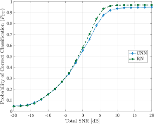
(a) Training and testing using DataSet1

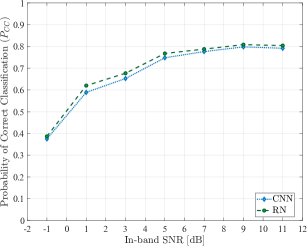
(b) Training and testing using DataSet2.

Figure 1: Classification performance of trained NNs when training and testing signals come from the same dataset.

When DataSet2 is used for NN training and testing, the corresponding probability of classification plot shown in Fig. 1(b) levels at a slightly lower value than when DataSet1 is used. This is because the two datasets are different, with more random variables in DataSet2 including a larger range of SRRC roll-off values, CFOs, randomized symbol rates, and signal power levels. Also, the architectures of the RN and CNN employed were very similar to those considered in [4] and have been optimized for DataSet1; further improvement on DataSet2 may be possible by changing the NN architecture.

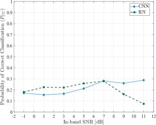
(a) Training using DataSet1, testing using DataSet2.

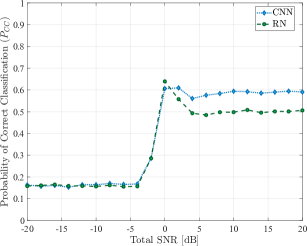
(b) Training using DataSet2, testing using DataSet1.

Figure 2: Classification performance of trained NNs when training and testing signals come from different datasets.

In the second experiment, we evaluated the performance of trained RN and CNN using test signals coming from a different dataset than the one used for training. Results from this experiment are shown in Fig. 2, from which it is apparent that the generalization performance of the trained NNs is poor, and that they fail to recognize digitally modulated signals belonging to classes they have been trained on when these signals come from a dataset that is different than the one the NNs have been trained on. We note that the use of DataSet1 for training the NNs does not seem to imply any generalization abilities as the corresponding probability of correct classification shown in Fig. 2(a) is essentially flat around $0.2$ for all SNR values. While we omit them from the presentation due to space constraints, confusion matrices for this case confirm that the NNs are not able to generalize and classify any of the modulation schemes for which they have been trained, when tested with signals that are not part of the training DataSet1.

When using DataSet2 for training the NNs, the corresponding probability of correct classification shown in Fig. 2(b) displays a jump around $0$ dB SNR from a low value of $0.2$ leveling at values around $0.5$ and $0.6$ for the RN and CNN, respectively. Thus, in this case, while the overall classification performance is below that obtained in the first experiment or reported in [4], the trained NNs seem to have some limited generalization ability, which may also be observed by looking at the corresponding confusion matrices. While these are omitted due to space constraints, we note that, out of the six modulation types which they have been trained to recognize, the RN continues to successfully classify $3$ (BPSK, QPSK, and 256-QAM), while the CNN recognizes $4$ (BPSK, QPSK, 8-PSK, and 256-QAM).

V Conclusions

The paper considers DL classification of digitally modulated signals using raw I/Q data and studies the generalization ability of NNs by evaluating their classification performance using signals that come from datasets they were not trained on. Results indicate that training a NN to perform modulation classification based on the raw I/Q data causes the NN to learn peculiarities of a particular training dataset, rather than conveying salient signal aspects that are determined by the underlying digital modulation scheme. Thus, more robust NN validation approaches, such as the one presented in this paper, should be used to ensure good classification performance.

To improve the generalization ability of NNs in classifying digitally modulated signals, future work will consider training them using specific signal features that can be extracted from the raw I/Q signal data, such as those based on cyclostationary signal processing.

References

- [1] J. L. Xu, W. Su, and M. Zhou, “Likelihood-Ratio Approaches to Automatic Modulation Classification,” IEEE Transactions on Systems, Man, and Cybernetics – Part C: Applications and Reviews, vol. 41, no. 4, pp. 3072–3108, July 2011.
- [2] F. Hameed, O. A. Dobre, and D. C. Popescu, “On the Likelihood-Based Approach to Modulation Classification,” IEEE Transactions on Wireless Communications, vol. 8, no. 12, pp. 5884–5892, December 2009.
- [3] C. M. Spooner, W. A. Brown, and G. K. Yeung, “Automatic Radio-Frequency Environment Analysis,” in Proceedings of the Thirty-Fourth Annual Asilomar Conference on Signals, Systems, and Computers, vol. 2, Monterey, CA, October 2000, pp. 1181–1186.
- [4] T. J. O’Shea, T. Roy, and T. C. Clancy, “Over-the-Air Deep Learning Based Radio Signal Classification,” IEEE Journal of Selected Topics in Signal Processing, vol. 12, no. 1, pp. 168–179, 2018.
- [5] T. O’Shea and J. Hoydis, “An Introduction to Deep Learning for the Physical Layer,” IEEE Transactions on Cognitive Communications and Networking, vol. 3, no. 4, pp. 563–575, 2017.
- [6] J. Sun, G. Wang, Z. Lin, S. G. Razul, and X. Lai, “Automatic Modulation Classification of Cochannel Signals using Deep Learning,” in Proceedings 23rd IEEE International Conference on Digital Signal Processing (DSP), 2018, pp. 1–5.
- [7] D. Zhang, W. Ding, C. Liu, H. Wang, and B. Zhang, “Modulated Autocorrelation Convolution Networks for Automatic Modulation Classification Based on Small Sample Set,” IEEE Access, vol. 8, pp. 27 097–27 105, 2020.
- [8] M. Kulin, T. Kazaz, I. Moerman, and E. De Poorter, “End-to-End Learning From Spectrum Data: A Deep Learning Approach for Wireless Signal Identification in Spectrum Monitoring Applications,” IEEE Access, vol. 6, pp. 18 484–18 501, 2018.
- [9] S. Rajendran, W. Meert, D. Giustiniano, V. Lenders, and S. Pollin, “Deep Learning Models for Wireless Signal Classification With Distributed Low-Cost Spectrum Sensors,” IEEE Transactions on Cognitive Communications and Networking, vol. 4, no. 3, pp. 433–445, 2018.
- [10] K. Bu, Y. He, X. Jing, and J. Han, “Adversarial Transfer Learning for Deep Learning Based Automatic Modulation Classification,” IEEE Signal Processing Letters, vol. 27, pp. 880–884, 2020.
- [11] J. Djolonga, J. Yung, M. Tschannen, and et al., “On Robustness and Transferability of Convolutional Neural Networks,” accessed: Feb. 18, 2021. [Online]. Available: https://arxiv.org/pdf/2007.08558.pdf.
- [12] DeepSig, Inc. RF Data Sets for Machine Learning: DeepSig Dataset RADIOML 2018.01A. Accessed Dec. 14, 2020. [Online]. Available: https://www.deepsig.ai/datasets.
- [13] The CSP Blog, “Data Set for the Machine Learning Challenge,” accessed Dec. 7, 2020. [Online]. Available: https://cyclostationary.blog/2019/02/15/data-set-for-the-machine-learning-challenge.
- [14] I. Goodfellow, Y. Bengio, and A. Courville, Deep Learning. MIT Press, 2016, https://www.deeplearningbook.org.