Using Rewrite Strategies for Efficient Functional Automatic Differentiation

Abstract.

Automatic Differentiation (AD) has become a dominant technique in ML. AD frameworks have first been implemented for imperative languages using tapes. Meanwhile, functional implementations of AD have been developed, often based on dual numbers, which are close to the formal specification of differentiation and hence easier to prove correct. But these papers have focussed on correctness not efficiency. Recently, it was shown how an approach using dual numbers could be made efficient through the right optimizations. Optimizations are highly dependent on order, as one optimization can enable another. It can therefore be useful to have fine-grained control over the scheduling of optimizations. One method expresses compiler optimizations as rewrite rules, whose application can be combined and controlled using strategy languages. Previous work describes the use of term rewriting and strategies to generate high-performance code in a compiler for a functional language. In this work, we implement dual numbers AD in a functional array programming language using rewrite rules and strategy combinators for optimization. We aim to combine the elegance of differentiation using dual numbers with a succinct expression of the optimization schedule using a strategy language. We give preliminary evidence suggesting the viability of the approach on a micro-benchmark.

1. Introduction

Training a neural network means optimizing the parameters which control its behavior, with respect to a loss function. The usually employed optimization algorithms, which are based on gradient descent, require computing the loss function’s gradient (Wang et al., 2018). This means that we need to differentiate the neural network. While this could in principle be done by hand, automatic differentiation (AD) allows computing the derivative of a given program without additional programming effort. As AD is not restricted to the specific operations used by typical neural networks, more complex constructs, for example involving control flow, can be employed in machine learning, as long as the program remains differentiable and has trainable parameters. This approach, which generalizes from deep neural networks to a broader class of programs, has been called differentiable programming (Yann LeCun, 2018).

Models in differentiable programming operate over nested arrays, or tensors. Hence, commonly used deep learning frameworks like PyTorch (Paszke et al., 2019) or JAX (Bradbury et al., 2018) feature a large number of built-in operations on tensors. In this work, we are instead interested in array languages which have only few built-in constructs upon which richer APIs can be constructed, like F̃ (Shaikhha et al., 2017, 2019) or Dex (Paszke et al., 2021). Our implementation of an array programming language as a domain specific language (DSL) closely follows the former.

Functional approaches to AD based on dual numbers can be conceptually simple and have been the basis of correctness proofs (Mazza and Pagani, 2021). There is a challenge when using this approach for ML: gradient descent needs the full gradient of the loss function. But dual numbers can only compute the gradient one entry at a time. The size of the gradient is equal to the number of parameters the model has, so differentiating over a model with $n$ parameters requires $n$ executions of the differentiated function.

To improve the performance of their dual numbers AD algorithm, Shaikhha et al. (2019) present a set of optimization rules. Optimizations are highly dependent on order, as one optimization can enable another. It can therefore be useful to have fine-grained control and explore different schedules for the optimization. One method expressing compiler optimizations as rewrite rules, whose application can be combined and controlled using strategy languages (Visser et al., 1998). Hagedorn et al. (2020) describes the use of term rewriting and strategies to generate high-performance code in a compiler for a functional language, but they did not model differentation.

Contributions

In this work, we implement dual numbers AD in a functional array programming language using rewrite rules and strategy combinators for optimization. We aim to combine the elegance of differentiation using dual numbers with a succinct expression of the optimization schedule using a strategy language. We give preliminary evidence suggesting the viability of the approach on a micro-benchmark. Our array language is implemented in the Lean programming language and theorem prover (de Moura and Ullrich, 2021) as an embedded DSL. We use Lean’s dependent types to track the sizes of arrays and indices in the type system, aiming to prevent out-of-bounds errors.

2. Language

$$n\in\mathds{Z}$$

$$\alpha,\beta ::=\alpha\to\beta~{}|~{}\alpha\times\beta~{}|~{}\mathtt{array}_{n}~{}\alpha~{}|~{}\mathtt{int}~{}|~{}\mathtt{fin}_{n}~{}|~{}\mathtt{real}$$

(a) Types.

$$\mathcal{D}\llbracket\alpha\to\beta\rrbracket~{}:=~{} \mathcal{D}\llbracket\alpha\rrbracket\to\mathcal{D}\llbracket\beta\rrbracket$$

$$\mathcal{D}\llbracket\alpha\times\beta\rrbracket~{}:=~{} \mathcal{D}\llbracket\alpha\rrbracket\times\mathcal{D}\llbracket\beta\rrbracket$$

$$\mathcal{D}\llbracket\mathtt{array}_{n}~{}\alpha\rrbracket~{}:=~{} \mathtt{array}_{n}~{}\mathcal{D}\llbracket\alpha\rrbracket$$

$$\mathcal{D}\llbracket\mathtt{int}\rrbracket~{}:=~{} \mathtt{int}$$

$$\mathcal{D}\llbracket\mathtt{fin}_{n}\rrbracket~{}:=~{} \mathtt{fin}_{n}$$

$${\color[rgb]{0,0,1}\mathcal{D}\llbracket\mathtt{real}\rrbracket~{}:=~{}} {\color[rgb]{0,0,1}\mathtt{real}\times\mathtt{real}}$$

(b) Dual numbers transformation on types.

Figure 1. Definition of types and dual numbers transformation.

x_α : α   f : α→β a : αf a : β   b : βλx_α . b : α→β   e_1 : α e_2 : βlet x_α := e_1; e_2 : β
c : int  e_1 : α e_2 : αif c then e_1 else e_2  f : α→fin_n →α x : αifold_n f x : α
n ∈Rn : real  i ∈Zi : int  i ∈{0,…,n-1}i : fin_n

$$\mathtt{mkpair} :\alpha\to\beta\to\alpha\times\beta$$

$$\mathtt{fst} :\alpha\times\beta\to\alpha$$

$$\mathtt{snd} :\alpha\times\beta\to\beta$$

$$\mathtt{geti_{n}} :\mathtt{array}_{n}~{}\alpha\to\mathtt{fin}_{n}\to\alpha$$

$$\mathtt{build_{n}} :(\mathtt{fin}_{n}\to\alpha)\to\mathtt{array}_{n}~{}\alpha$$

$$+ :\mathtt{real}\to\mathtt{real}\to\mathtt{real}$$

$$* :\mathtt{real}\to\mathtt{real}\to\mathtt{real}$$

$$\char 60\relax :\mathtt{real}\to\mathtt{real}\to\mathtt{int}$$

$$= :\mathtt{int}\to\mathtt{int}\to\mathtt{int}$$

(a) Terms.

$$\mathcal{D}\llbracket x_{\alpha}\rrbracket~{}:=~{} x_{\mathcal{D}\llbracket\alpha\rrbracket}$$

$$\mathcal{D}\llbracket e_{1}e_{2}\rrbracket~{}:=~{} \mathcal{D}\llbracket e_{1}\rrbracket\mathcal{D}\llbracket e_{2}\rrbracket$$

$$\mathcal{D}\llbracket\lambda x_{\alpha}.~{}e\rrbracket~{}:=~{} \lambda x_{\mathcal{D}\llbracket\alpha\rrbracket}.~{}\mathcal{D}\llbracket e\rrbracket$$

$$\mathcal{D}\llbracket\mathtt{let}~{}x_{\alpha}:=e_{1};~{}e_{2}\rrbracket~{}:=~{} \mathtt{let}~{}x_{\mathcal{D}\llbracket\alpha\rrbracket}:=\mathcal{D}\llbracket e_{1}\rrbracket;~{}\mathcal{D}\llbracket e_{2}\rrbracket$$

$$\mathcal{D}\llbracket\mathtt{if}~{}c~{}\mathtt{then}~{}e_{1}~{}\mathtt{else}~{}e_{2}\rrbracket~{}:=~{} \mathtt{if}~{}\mathcal{D}\llbracket c\rrbracket~{}\mathtt{then}~{}\mathcal{D}\llbracket e_{1}\rrbracket~{}\mathtt{else}~{}\mathcal{D}\llbracket e_{2}\rrbracket$$

$$\mathcal{D}\llbracket\mathtt{ifold}_{n}~{}f~{}x\rrbracket~{}:=~{} \mathtt{ifold}_{n}~{}\mathcal{D}\llbracket f\rrbracket~{}\mathcal{D}\llbracket x\rrbracket$$

$${\color[rgb]{0,0,1}\mathcal{D}\llbracket n:\mathtt{real}\rrbracket~{}:=~{}} {\color[rgb]{0,0,1}(n,0)}$$

$${\color[rgb]{0,0,1}\mathcal{D}\llbracket+\rrbracket~{}:=~{}} {\color[rgb]{0,0,1}\lambda x~{}y.~{}(x_{1}+y_{1},x_{2}+y_{2})}$$

$${\color[rgb]{0,0,1}\mathcal{D}\llbracket*\rrbracket~{}:=~{}} {\color[rgb]{0,0,1}\lambda x~{}y.~{}(x_{1}+y_{1},x_{1}*y_{2}+x_{2}*y_{1})}$$

$${\color[rgb]{0,0,1}\mathcal{D}\llbracket\char 60\relax\rrbracket~{}:=~{}} {\color[rgb]{0,0,1}\lambda x~{}y.~{}x_{1}\char 60\relax y_{1}}$$

$$\mathcal{D}\llbracket i:\mathtt{int}\rrbracket~{}:=~{} i$$

$$\mathcal{D}\llbracket i:\mathtt{fin}_{n}\rrbracket~{}:=~{} i$$

$$\mathcal{D}\llbracket\mathtt{mkpair}\rrbracket~{}:=~{} \mathtt{mkpair}$$

$$\mathcal{D}\llbracket\mathtt{fst}\rrbracket~{}:=~{} \mathtt{fst}$$

$$\mathcal{D}\llbracket\mathtt{snd}\rrbracket~{}:=~{} \mathtt{snd}$$

$$\mathcal{D}\llbracket\mathtt{geti}_{n}\rrbracket~{}:=~{} \mathtt{geti}_{n}$$

$$\mathcal{D}\llbracket\mathtt{build}_{n}\rrbracket~{}:=~{} \mathtt{build}_{n}$$

$$\mathcal{D}\llbracket=\rrbracket~{}:=~{} =$$

(b) Dual numbers transformation on terms.

Figure 2. Definition of terms and dual numbers transformation.

For writing models as well as optimization and code generation, we use an intrinsically typed deep embedding. The definition of the types is found in Figure 1(a). Our language has pairs, functions and length-indexed arrays. The base types are integers, size-bounded natural numbers and real numbers.

We use a limited form of dependent types: array types carry not only the type of the array’s elements, but also the array’s length. This means that, for example, the type $\mathtt{array}_{5}\mathtt{int}$ represents arrays of five integers. Additionally, we use the type $\mathtt{fin}_{n}$ for indices which represents integers in the range 0..n-1. To retrieve an element from an array of type $\mathtt{array}_{n}\mathtt{int}$, we require the index to be of type $\mathtt{fin}_{n}$. This is intended to prevent out-of-bounds array accesses. This is similar to the approach used in the Dex array language (Paszke et al., 2021).

Figure 2(a) shows the terms of the language. The language is intrinsically typed — Term carries a parameter representing the type of the expression. Instead of defining the syntax and the type system separately, the language’s constructs are always typed and creating an ill-typed expression is impossible. The typing rules do not use contexts; instead, each variable is labeled by its type (Church, 1940).

The terms are variables, function application, let-bindings, pair construction and projection, if-then-else, iteration, constants for real numbers, integers and indices as well as pre-defined operations for array construction and indexing, arithmetic, equality checking and conversion. Every variable consists of its name and its type. The typing rule for function application expects a function of type $\alpha\to\beta$ and an argument of type $\alpha$ and yields a term of type $\beta$. The abstraction case is based on the typing rule for lambda abstractions. Note that we again have to give both a name and a type for each variable. letin is similar to lam in that it also binds a variable, except we also already give the value that the variable should be bound to. mkpair is used to build pairs and fst and snd are used to take them apart. We can perform branching with if c then e1 else e2, evaluating the first branch if the condition is not zero, and the second otherwise. ifold allows bounded iteration. The fact that the loop index has type fin n is important when using it to access an array’s elements, for example when computing the sum of an array. The array operations build, for constructing arrays, and geti, for accessing elements, are now dependently typed. This means that geti cannot go out of bounds. The types of the two operations also reveal that they are essentially conversion functions, where build converts from fin n $\scriptstyle\sim$> a to array n a and geti converts back. There is no length operation; as the type of an array expression now carries its size, length is superfluous. We also have arithmetic operations.

3. Automatic Differentiation

The first step in our implementation of AD is a dual numbers transformation (Shaikhha et al., 2019). As can be seen in Figure 1(b), it is structurally recursive and transforms every occurrence of a real number into a pair of real numbers and leaves other type constructors unchanged. The idea is that each value is bundled with its derivative with regards to some input, so that both the normal result of the computation and the derivative are computed at the same time.

The transformation on terms is defined in Figure 2(b). Its structure follows the structure of the type transformation in that most of the cases of the transformation are trivial, except for those referring to real numbers. Variables have only their type changed. Similarly, the transformation on function application, $\lambda$-abstraction, if-then-else and iteration leaves their structure unchanged and simply recursively applies the transformation on the subexpressions. For the cases for addition and multiplication of real numbers, note that we write $(x,y)$ as shorthand for $\mathtt{mkpair}~{}x~{}y$ and $x_{1}$ and $x_{2}$ as shorthand for $\mathtt{fst}~{}x$ and $\mathtt{snd}~{}x$. Other operations are unchanged, e.g. operations on pairs (like fst), arrays (like build), or integers (like addInt, = or fromInt). This corresponds to the intuition that we actually just want to replace constants and arithmetic operations with their dual numbers equivalents.

In the case of comparisons like $\char 60\relax$, the transformed version simply retrieves the primal values from the dual numbers given as input and performs the comparison on those. As Boolean operators are not differentiable, the perturbations of the input numbers are simply discarded.

With the dual numbers transformation defined, we now want to use it to compute the gradient of a given model. The AD operators defined here are inspired by Shaikhha et al. (2019).

$$\mathtt{addZeroes}~{}(v:\mathtt{Array}_{n}~{}\alpha):\mathtt{Array}_{n}~{}(\alpha\times\mathtt{real}):=$$

$$\quad\mathtt{build}_{|v|}~{}(\lambda i.~{}(v[i],0))$$

$$\mathtt{zip}~{}(v_{1}:\mathtt{Array}_{n}~{}\alpha)~{}(v_{2}:\mathtt{Array}_{n}~{}\beta):\mathtt{Array}_{n}~{}(\alpha\times\beta):=$$

$$\quad\mathtt{build}_{n}~{}(\lambda i.~{}(v_{1}[i],v_{2}[i]))$$

The helper function addZeroes transforms an array of real numbers into an array of dual numbers by using each input number as the primal and setting the perturbation to zero, while zip combines two arrays of equal length into one.

$$\mathtt{oneHot}_{n}~{}i:=\mathtt{build}_{n}~{}(\lambda j.~{}\mathtt{if}~{}i=j~{}\mathtt{then}~{}1~{}\mathtt{else}~{}0)$$

$$\mathtt{lossDiff}~{}e~{}x~{}y~{}p~{}\bar{p}:$$

$$\quad(\mathtt{Array}_{a}~{}\mathtt{real}\to\mathtt{Array}_{b}~{}\mathtt{real}\to\mathtt{Array}_{n}~{}\mathtt{real}\to\mathtt{real})\to$$

$$\quad\mathtt{Array}_{a}~{}\mathtt{real}\to\mathtt{Array}_{b}~{}\mathtt{real}\to\mathtt{Array}_{n}~{}\mathtt{real}\to$$

$$\quad\mathtt{Array}_{n}~{}\mathtt{real}\to\mathtt{real}:=$$

$$\quad\mathtt{snd}~{}(\mathcal{D}\llbracket e\rrbracket~{}(\mathtt{addZeroes}~{}x)~{}(\mathtt{addZeroes}~{}y)~{}(\mathtt{zip}~{}p~{}\bar{p}))$$

lossDiff computes the directional derivative. It assumes as its argument a loss function that takes three arguments: an input from the dataset, the corresponding output and the current parameters of the model. The loss function then returns a number denoting the difference between the model’s output and the true output.

$$\mathtt{oneHot}_{n}~{}i:=\mathtt{build}_{n}~{}(\lambda j.~{}\mathtt{if}~{}i=j~{}\mathtt{then}~{}1~{}\mathtt{else}~{}0)$$

$$\mathtt{lossGrad}~{}e~{}x~{}y~{}p:$$

$$\quad(\mathtt{Array}_{a}~{}\mathtt{real}\to\mathtt{Array}_{b}~{}\mathtt{real}\to\mathtt{Array}_{n}~{}\mathtt{real}\to\mathtt{real})\to$$

$$\quad\mathtt{Array}_{a}~{}\mathtt{real}\to\mathtt{Array}_{b}~{}\mathtt{real}\to\mathtt{Array}_{n}~{}\mathtt{real}\to$$

$$\quad\mathtt{Array}_{n}~{}\mathtt{real}:=$$

$$\quad\mathtt{build}_{|p|}~{}(\lambda i.~{}\mathtt{lossDiff}~{}e~{}x~{}y~{}p~{}(\mathtt{oneHot}_{|p|}i))$$

lossGrad computes the full gradient. It calls lossDiff multiple times using a one-hot encoding, given by oneHot. On each call, one entry of the gradient is computed. This implies a number of executions equal to the dimension of the parameter vector.

4. Implementation

Our implementation is written in Lean, a functional programming language and theorem prover (de Moura and Ullrich, 2021). We give a short overview of our implementation.

We define terms as a generalized algebraic data type (inductive). We will omit most of the cases; they are unsurprising and follow the definition given in Fig. 1(b).

⬇

inductive Term : Typ → Type

| var (x:String) (a) : Term a

| app : Term (a ~> b) → Term a → Term b

| lam (x:String) (a) {b} : Term b → Term (a ~> b)

The dual numbers transformation is defined as a recursive function operating on the data type.

⬇

def diff : Term a → Term a.diff

| var x a => var x a.diff

| app e1 e2 => app e1.diff e2.diff

| lam x _ e => lam x _ e.diff

Lean also features dependent types, which are types that depend on values. One example of a dependent type is Fin n, intuitively the type of numbers from $0$ to $n-1$. Note that type constructors like Fin are just functions from types to types, so we can define them the same way we define other functions.

⬇

def Fin (n : Nat) : Type := {i : Nat // i < n}

The notation on the right-hand side is akin to set builder notation. It can be read as referring to the type of all natural numbers i such that i < n. More precisely, it is the type consisting of pairs where the first element is a number i and the second element is a proof of the proposition i < n.

The fact that Lean is dependently typed allows for a very simple implementation of size-typed arrays and indices, as can be seen in the definition of (a subset of) the types of our DSL:

⬇

inductive Typ

| real : Typ

| array : Nat → Typ → Typ

| fin : Nat → Typ

Both array and fin are size-typed by indexing them with a natural number representing the size.

It may seem that Term is quite limited in its expressivity. The language is simply typed and size parameters for arrays and indices have to be constants. We can however represent functions that are polymorphic both over types and over array sizes by quantifying on the level of the metalanguage, Lean. Consider, for example, the function vectorMap, which applies a function to every element of an array.

⬇

def vectorMap {n : Nat} {a b : Typ} :

Term (array n a ~> (a ~> b) ~> array n b) :=

lam ”v” _ (lam ”f” _

(build’ (lam ”i” _ (app ”f” (geti’ (var ”v” (array n a)) ”i”)))))

It is polymorphic with regards to the size of the array as well as to the type of the function and the array’s elements. This is represented by a Lean function that takes a number (the size parameter) and two values of type Typ (the type parameters) as input and returns an Term expression. This way, polymorphic functions can be specialized to concrete, monomorphic ones. The concrete types can often be inferred from the context by the Lean type checker.

5. Optimization

We want to implement rewrite rules and the following optimization strategies, based on Visser et al. (1998), in code.

(identifiers) $x$    (rules) $r$

$$\text{(strategies)}~{}s::=x~{}|~{}r~{}|~{}\mathsf{id}~{}|~{}\lightning~{}|~{}s_{1};\;s_{2}~{}|~{}s_{1}\mathrel{\mkern 8.0mu\vbox{\hbox{$\scriptscriptstyle+$}}\mkern-17.0mu{\leftarrow}}s_{2}~{}|~{}\mu x.~{}s~{}|~{}\diamond(s)$$

Strategies can be seen as procedures that try to transform terms and either succeed, returning a new term, or fail. First, every rewrite rule can be seen as a strategy that, given a term $t$, succeeds if the rule can be applied to $t$ at the root (so there is no nondeterminism here, as we do not apply rules to subterms). We also have the identity strategy id, which always succeeds, leaving the term unchanged. On the other hand, the strategy $\lightning$ always fails. We write $s_{1};s_{2}$ to denote the sequential composition of two strategies $s_{1}$ and $s_{2}$. Strategy $s_{1}$ is applied first, and if it succeeds, $s_{2}$ is applied to the result. If either $s_{1}$ or $s_{2}$ fails, $s_{1};s_{2}$ fails. Left choice $s_{1}\mathrel{\mkern 8.0mu\vbox{\hbox{$\scriptscriptstyle+$}}\mkern-17.0mu{\leftarrow}}s_{2}$ first attempts to apply $s_{1}$. If the strategy $s_{1}$ succeeds, its output is returned is the output of $s_{1}\mathrel{\mkern 8.0mu\vbox{\hbox{$\scriptscriptstyle+$}}\mkern-17.0mu{\leftarrow}}s_{2}$. If it fails, $s_{2}$ is applied on the term. We also have the fixed point operator $\mu$, which allows us to define recursive strategies.

We also make use of the following, derived, operation:

$$\text{repeat}(s):=\mu x.~{}((s;x)\mathrel{\mkern 8.0mu\vbox{\hbox{$\scriptscriptstyle+$}}\mkern-17.0mu{\leftarrow}}\mathsf{id})$$

$\text{repeat}(s)$ iteratively applies a strategy $s$ as often as possible and stops once $s$ fails. Note that $\text{repeat}(s)$ can never fail; however it may loop indefinitely. For example, because id never fails, $\text{repeat}(\mathsf{id})$ does not terminate on any input term. As rules are only applied to the root, we need a way to rewrite the subterms of a given term. This is addressed by the $\diamond$ operator. A strategy $\diamond(s)$ tries to apply $s$ to exactly one subterm of the given term and fails if there is no subterm to which $s$ can be applied successfully.

In a functional programming language, this can be done by representing strategies as functions and combinators as higher-order functions which take and return strategies. Most of the combinators defined in this section are based on those of the ELEVATE strategy language (Hagedorn et al., 2020), which is itself inspired by Stratego (Visser, 2005; Visser et al., 1998).

The type of an expressions is Term a for some a. What should the type of a strategy look like? The type Term a → Term a seems sensible, but it assumes that strategies always produce an expression. Strategies may, however, fail. So an improved type would be Term a → Option (Term a), where a value of type Option (Term a) can either be none, representing failure, or some x (where x is of type Term a), representing success. In our case, this leaves one issue open. We need to be able to generate fresh variable names (as part of capture-avoiding substitution, for example). How can we do this in a purely functional language? The answer is to combine Option with the state monad, which allows us to thread a state through our computation. In this case, the state is a natural number which serves as a counter that is incremented whenever a new variable is produced. The counter is then used as part of the returned variable name.

This leads us to the following definitions:

⬇

def RewriteResult a : Type := Nat → Option (a × Nat)

The meaning of RewriteResult is that it represents a computation which takes a counter value and then either fails or returns an output, together with a new, possibly increased counter value. It is a monad, allowing the use of do-notation.
A strategy is then a function taking an expression and returning a RewriteResult, while preserving the type of the expression.

⬇

def Strategy : Type :=

{a:Typ} → Term a → RewriteResult (Term a)

We can now define a function freshM, which returns a variable name based on the current counter and increments said counter:

⬇

def freshM : RewriteResult String

| i => some (”x” ++ toString i, i+1)

We now implement the strategy combinators. First we have id, which takes a term and a counter and returns both unchanged.

⬇

def id : Strategy := fun p i => some (p, i)

Failure $\lightning$ is implemented as a function fail, which always returns none.

⬇

def fail : Strategy := fun _ _ => none

Sequencing $s_{1};\;s_{2}$ is represented as seq s1 s2 (abbreviated as s1 ;; s2). The code uses do-notation to first apply strategy s1 to term p, and then, on success, s2.

⬇

def seq (s1 s2 : Strategy) : Strategy :=

fun p => do s2 (← s1 p)

We write left choice $s_{1}\mathrel{\mkern 8.0mu\vbox{\hbox{$\scriptscriptstyle+$}}\mkern-17.0mu{\leftarrow}}s_{2}$ as lchoice s1 s2 (abbreviated as s1 <+ s2). The implementation uses the <|> operator, which takes two computations and returns the result of the left one if it succeeds, and that of the right one otherwise.

⬇

def lchoice (s1 s2 : Strategy) : Strategy :=

fun p => s1 p <|> s2 p

We do not introduce a fixed point construct $\mu x.~{}s$, rather, we define strategies recursively using Lean’s support for recursive definitions. This can be seen in the definition of $\text{repeat}(s)$.

⬇

partial def repeat (s : Strategy) : Strategy

| _, p => ((s ;; repeat s) <+ id) p

Lean requires us to add the partial keyword before def, indicating that we cannot guarantee termination.

We now consider traversals, which are functions that transform strategies to allow us to rewrite subexpressions of the current expression.

⬇

def Traversal := Strategy → Strategy

For each constructor in the language, we define traversals for each subexpression of that constructor. For the function application constructor app, which contains two subexpressions (function and argument), we need two traversals: function s, which applies s to the first subexpression, and argument s, which applies it to the second. If function s or argument s are applied to anything other than a function application, they fail.

⬇

def function : Traversal

| s, _, app f a => do return app (<- s f) a

| _, _, _ => failure

def argument : Traversal

| s, _, app f a => do return app f (<- s a)

| _, _, _ => failure

The same way, we define traversals for the other constructors, one for each of their respective subexpressions.

We can now implement the combinator one s ($\diamond s$), which applies s to one subexpression. The implementation given here is deterministic, as it is biased towards the subexpression on the left. one works by trying to apply $s$ to every type of subexpression in order.

⬇

def one (s : Strategy) : Strategy :=

function s <+ argument s <+ – other traversals omitted

one by itself only allows us do transform expressions that are direct subexpressions of the root of the abstract syntax tree. To allow transformations of more deeply nested expressions, we define the recursive topDown traversal. topDown s first tries to apply s at the root and if that fails, recurses into the subexpressions until it finds one expression where s succeeds.

⬇

partial def topDown : Traversal :=

fun s => s <+ one (topDown s)

Combining topDown with repeat, we get normalize s, which repeatedly applies s until there is no subexpression left to be transformed.

⬇

def normalize (s : Strategy) : Strategy :=

repeat (topDown s)

We also define run, which lets us execute a strategy on a term, by initializing the variable counter to 0, applying the strategy, and then discarding the new counter at the end.

⬇

def run : Strategy → Term a → Option (Term a)

| s, p => Prod.fst <$> s p 0

5.1. Efficient AD

Deriving the gradient of a function $f$ via forward mode AD involves $n$ computations of the function, where $n$ is the size of $f$’s input vector. This would appear to make forward mode AD unusable for training large machine learning models.

To address this, Shaikhha et al. (2019) present a set of rewrite rules. Using these to optimize their programs, they are able to achieve performance on their benchmarks that is competitive with or superior to frameworks using reverse mode AD. We can implement these rules as functions of the Strategy type, using pattern matching.

As an example consider the following rule, where constructing an array and immediately retrieving a single element from it is optimized to a simple function application.

⬇

def getBuild : Strategy

| _, geti’ (build’ e1) e2 => return app e1 e2

| _, _ => failure

The correctness of the rule follows from the following equality that holds in the semantics (not shown) of our DSL.

$$\mathtt{geti}~{}(\mathtt{build}~{}e_{1})~{}e_{2}\quad\equiv\quad e_{1}~{}e_{2}$$

The intuition is that $\mathtt{build}~{}e_{1}$ constructs an array that maps an index $i$ to $e_{1}~{}i$ and therefore, indexing this array with $e_{2}$ gives $e_{1}~{}e_{2}$.

Shaikhha et al. also use a rule for removing let-bindings by substituting the bound variable:

$$\mathtt{let}~{}x_{\alpha}:=e_{1};~{}e_{2}\quad\equiv\quad e_{1}[x_{a}:=e_{2}]$$

In Lean, it looks like this:

⬇

def letSubst : Strategy

| _, letin x a e1 e2 => subst y a e1 e2

| _, _ => failure

This may duplicate work if y is used multiple times in e1. So we use the following strategy, where count (freeVars e1) (y, a) returns the number of times that the variable occurs free in e1. The strategy letSubstN only substitutes if the variable does not occur more often than a given threshold. We use a treshold of 1. This prevents the substitution from duplicating expressions, which could lead to an exponential slowdown.

⬇

def letSubstN (n : Nat): Strategy

| _, letin y a e0 e1 =>

if count (freeVars e1) (y, a) <= n

then subst y a e0 e1

else failure

| _, _ => failure

Substitution in the lambda calculus is subtle; renaming variables may be necessary to avoid name captures (Mimram, 2020). We address this by using the ”sledge-hammer [sic] approach” described by Jones and Marlow (2002): before substitution, rename every bound variable in the term you are substituting for the variable. This is done using the freshTerm strategy, which makes use of the RewriteResult monad to generate fresh variables through the freshM function. The case for lam contains the expression replaceVar y x a b’, which evaluates to the result of replacing each occurrence of var y a with var x a in b’.

⬇

def freshTerm : Strategy

| _, var y a => return var y a

| _, lam y a b => do

let b’ ← freshTerm b

let x ← freshM

return lam x a (replaceVar y x a b’)

| _, app f a =>

do return app (<- freshTerm f) (<- freshTerm a)

– omitted letin and mkpair for brevity

| _, e => return e

6. Evaluation

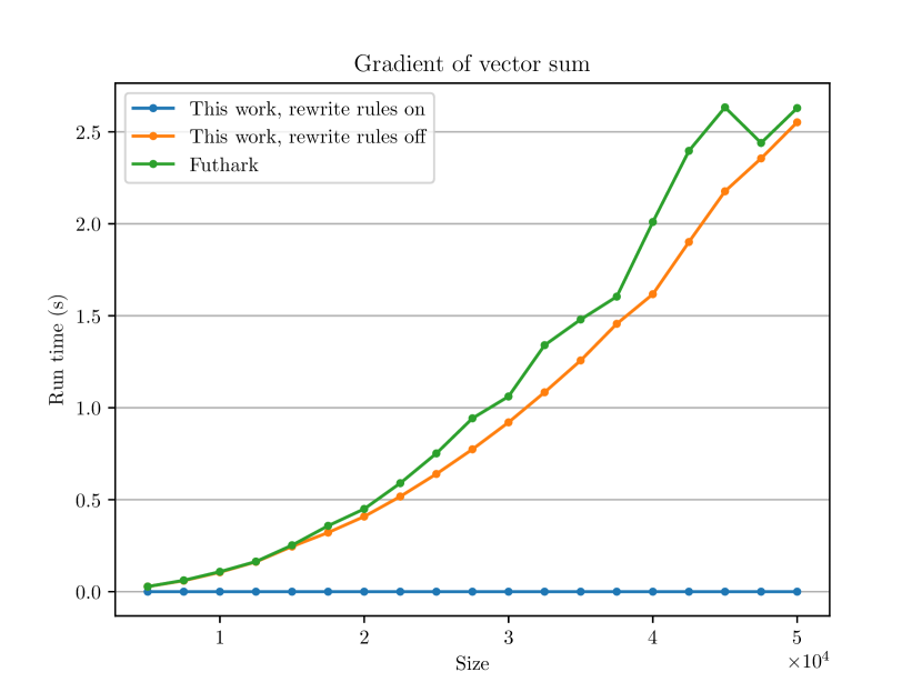
(a) Comparison between the optimized and unoptimized programs.

(b) Performance of the optimized program.

Figure 3. Results of the vector sum benchmark.

We conducted a micro-benchmark to test the performance of our implementation to measure the impact of the optimization rules. For the benchmarks we use Python 3.6.9, Futhark 0.22.0, and gcc 7.5.0. The execution is done on a Intel Pentium G860 (3GHz) with 4GB of memory. Our implementation converts the terms to a string representing Futhark (Henriksen et al., 2017) code, which is then compiled by the Futhark compiler. We use the Futhark compiler’s C backend.

The micro-benchmark consists of a very simple program which first generates an array of a given length where every entry is the same constant value and then computes the gradient of vectorSum on that array, where vectorSum is a function that sums all the entries of an array. This program is somewhat trivial, in that the vectorSum function is linear and therefore the gradient is always an array consisting of only 1s. This benchmark should merely demonstrate that the optimizations from Sec. 5.1 can in principle lead to asymptotic speedups.

We tested three different versions. First, a program that is compiled to Futhark with no optimizations applied before compilation. Second, the same program with optimizations applied before compilation to Futhark. Due to technical issues with compilation, the unoptimized program is generated from the typed embedding while the optimized one is generated from an untyped one. This should not affect the qualitative observations we make about the results. Third, we have a hand-written Futhark program, using a dual numbers library to implement forward mode AD.

We measured execution time for vector sizes from 2500 to 50000. The results can be seen in Figure 3. We give one plot comparing the three programs and another one focussing only on the runtime of our optimized one.

The left plot shows that the runtime for the unoptimized program in our DSL (orange) increases faster than linearly. This is expected, as forward mode AD leads to an overhead proportional to the size of the input vector. It can be seen however, that the optimized program (blue) is asymptotically faster than the unoptimized one. The rewrite rules are able to optimize away the nested loops involved in computing the gradient of vectorSum.

Additionally, the hand-written Futhark program (green) is also asymptotically slower than the optimized one. As all three versions are compiled by the optimizing Futhark compiler, this demonstrates that we were able to express application-specific optimizations for differentiability in our strategy-based approach which are not included in the fixed optimization passes of the Futhark compiler.

7. Related Work

Forward-mode AD tends to be implemented with dual numbers. Alternatively, reverse-mode AD allows computing the gradient in one execution, but incurs a complication, as the control flow for computing the derivative has to be inverted. Some reverse-mode AD frameworks are implemented as non-compositional transformations, including Zygote (Innes, 2018) for Julia, Enzyme (Moses and Churavy, 2020) for LLVM, and Tapenade (Hascoët and Pascual, 2013) for Fortran and C. These lack correctness proofs. Reverse-mode AD has also been implemented compositionally with continuations (Wang et al., 2018) or effect handlers (de Vilhena and Pottier, 2021) as well as mutable state, which may require advanced techniques like separation logic to verify. An abstract description of differentiation is given by categorical models of differentation (Blute et al., 2009; Bucciarelli et al., 2010; Cockett et al., 2020). These do not directly yield an AD algorithm, but can be used to verify one, as has been done by Cruttwell et al. (2020). Another compositional approach comes from Elliott (Elliott, 2018), who implements reverse-mode AD for a first-order language by reifying and transposing the derivative. Mazza and Pagani (2021) verify the correctness of AD for a Turing-complete higher-order functional language, but use an inefficient algorithm. We instead apply a forward-mode transformation and recover efficiency by optimizing the code afterwards, making use of the flexibility of rewrite strategies.

8. Conclusion

We described the implementation of a higher-order functional array language supporting differentiable programming. Previous work (Shaikhha et al., 2019), has not expressed optimizations on differentiated programs using rewrite strategy languages (Visser et al., 1998; Hagedorn et al., 2020) and rewrite strategy languages have not been used for optimizing AD. We showed the effect of the optimizations on a micro-benchmark.

- (1)
- Blute et al. (2009) Richard F Blute, J Robin B Cockett, and Robert AG Seely. 2009. Cartesian differential categories. Theory and Applications of Categories 22, 23 (2009), 622–672.
- Bradbury et al. (2018) James Bradbury, Roy Frostig, Peter Hawkins, Matthew James Johnson, Chris Leary, Dougal Maclaurin, George Necula, Adam Paszke, Jake VanderPlas, Skye Wanderman-Milne, and Qiao Zhang. 2018. JAX: composable transformations of Python+NumPy programs. http://github.com/google/jax
- Bucciarelli et al. (2010) Antonio Bucciarelli, Thomas Ehrhard, and Giulio Manzonetto. 2010. Categorical Models for Simply Typed Resource Calculi. In Proceedings of the 26th Conference on the Mathematical Foundations of Programming Semantics, MFPS 2010, Ottawa, Ontario, Canada, May 6-10, 2010 (Electronic Notes in Theoretical Computer Science, Vol. 265), Michael W. Mislove and Peter Selinger (Eds.). Elsevier, 213–230. https://doi.org/10.1016/j.entcs.2010.08.013
- Church (1940) Alonzo Church. 1940. A Formulation of the Simple Theory of Types. J. Symb. Log. 5, 2 (1940), 56–68. https://doi.org/10.2307/2266170
- Cockett et al. (2020) J. Robin B. Cockett, Geoff S. H. Cruttwell, Jonathan Gallagher, Jean-Simon Pacaud Lemay, Benjamin MacAdam, Gordon D. Plotkin, and Dorette Pronk. 2020. Reverse Derivative Categories. In 28th EACSL Annual Conference on Computer Science Logic, CSL 2020, January 13-16, 2020, Barcelona, Spain (LIPIcs, Vol. 152), Maribel Fernández and Anca Muscholl (Eds.). Schloss Dagstuhl - Leibniz-Zentrum für Informatik, 18:1–18:16. https://doi.org/10.4230/LIPIcs.CSL.2020.18
- Cruttwell et al. (2020) Geoffrey S. H. Cruttwell, Jonathan Gallagher, and Dorette Pronk. 2020. Categorical semantics of a simple differential programming language. In Proceedings of the 3rd Annual International Applied Category Theory Conference 2020, ACT 2020, Cambridge, USA, 6-10th July 2020 (EPTCS, Vol. 333), David I. Spivak and Jamie Vicary (Eds.). 289–310. https://doi.org/10.4204/EPTCS.333.20
- de Moura and Ullrich (2021) Leonardo de Moura and Sebastian Ullrich. 2021. The Lean 4 Theorem Prover and Programming Language. In Automated Deduction - CADE 28 - 28th International Conference on Automated Deduction, Virtual Event, July 12-15, 2021, Proceedings (Lecture Notes in Computer Science, Vol. 12699), André Platzer and Geoff Sutcliffe (Eds.). Springer, 625–635. https://doi.org/10.1007/978-3-030-79876-5_37
- de Vilhena and Pottier (2021) Paulo Emílio de Vilhena and François Pottier. 2021. Verifying an Effect-Handler-Based Define-By-Run Reverse-Mode AD Library. arXiv preprint arXiv:2112.07292 (2021).
- Elliott (2018) Conal Elliott. 2018. The simple essence of automatic differentiation. Proc. ACM Program. Lang. 2, ICFP (2018), 70:1–70:29. https://doi.org/10.1145/3236765
- Hagedorn et al. (2020) Bastian Hagedorn, Johannes Lenfers, Thomas Koehler, Xueying Qin, Sergei Gorlatch, and Michel Steuwer. 2020. Achieving high-performance the functional way: a functional pearl on expressing high-performance optimizations as rewrite strategies. Proc. ACM Program. Lang. 4, ICFP (2020), 92:1–92:29. https://doi.org/10.1145/3408974
- Hascoët and Pascual (2013) Laurent Hascoët and Valérie Pascual. 2013. The Tapenade automatic differentiation tool: Principles, model, and specification. ACM Trans. Math. Softw. 39, 3 (2013), 20:1–20:43. https://doi.org/10.1145/2450153.2450158
- Henriksen et al. (2017) Troels Henriksen, Niels G. W. Serup, Martin Elsman, Fritz Henglein, and Cosmin E. Oancea. 2017. Futhark: purely functional GPU-programming with nested parallelism and in-place array updates. In Proceedings of the 38th ACM SIGPLAN Conference on Programming Language Design and Implementation, PLDI 2017, Barcelona, Spain, June 18-23, 2017, Albert Cohen and Martin T. Vechev (Eds.). ACM, 556–571. https://doi.org/10.1145/3062341.3062354
- Innes (2018) Michael Innes. 2018. Don’t Unroll Adjoint: Differentiating SSA-Form Programs. CoRR abs/1810.07951 (2018). arXiv:1810.07951 http://arxiv.org/abs/1810.07951
- Jones and Marlow (2002) Simon L. Peyton Jones and Simon Marlow. 2002. Secrets of the Glasgow Haskell Compiler inliner. J. Funct. Program. 12, 4&5 (2002), 393–433. https://doi.org/10.1017/S0956796802004331
- Mazza and Pagani (2021) Damiano Mazza and Michele Pagani. 2021. Automatic differentiation in PCF. Proc. ACM Program. Lang. 5, POPL (2021), 1–27. https://doi.org/10.1145/3434309
- Mimram (2020) Samuel Mimram. 2020. PROGRAM = PROOF.
- Moses and Churavy (2020) William S. Moses and Valentin Churavy. 2020. Instead of Rewriting Foreign Code for Machine Learning, Automatically Synthesize Fast Gradients. In Advances in Neural Information Processing Systems 33: Annual Conference on Neural Information Processing Systems 2020, NeurIPS 2020, December 6-12, 2020, virtual, Hugo Larochelle, Marc’Aurelio Ranzato, Raia Hadsell, Maria-Florina Balcan, and Hsuan-Tien Lin (Eds.). https://proceedings.neurips.cc/paper/2020/hash/9332c513ef44b682e9347822c2e457ac-Abstract.html
- Paszke et al. (2019) Adam Paszke, Sam Gross, Francisco Massa, Adam Lerer, James Bradbury, Gregory Chanan, Trevor Killeen, Zeming Lin, Natalia Gimelshein, Luca Antiga, Alban Desmaison, Andreas Köpf, Edward Z. Yang, Zachary DeVito, Martin Raison, Alykhan Tejani, Sasank Chilamkurthy, Benoit Steiner, Lu Fang, Junjie Bai, and Soumith Chintala. 2019. PyTorch: An Imperative Style, High-Performance Deep Learning Library. In Advances in Neural Information Processing Systems 32: Annual Conference on Neural Information Processing Systems 2019, NeurIPS 2019, December 8-14, 2019, Vancouver, BC, Canada, Hanna M. Wallach, Hugo Larochelle, Alina Beygelzimer, Florence d’Alché-Buc, Emily B. Fox, and Roman Garnett (Eds.). 8024–8035. https://proceedings.neurips.cc/paper/2019/hash/bdbca288fee7f92f2bfa9f7012727740-Abstract.html
- Paszke et al. (2021) Adam Paszke, Daniel D. Johnson, David Duvenaud, Dimitrios Vytiniotis, Alexey Radul, Matthew J. Johnson, Jonathan Ragan-Kelley, and Dougal Maclaurin. 2021. Getting to the point: index sets and parallelism-preserving autodiff for pointful array programming. Proc. ACM Program. Lang. 5, POPL (2021), 1–29. https://doi.org/10.1145/3473593
- Shaikhha et al. (2017) Amir Shaikhha, Andrew W. Fitzgibbon, Simon Peyton Jones, and Dimitrios Vytiniotis. 2017. Destination-passing style for efficient memory management. In Proceedings of the 6th ACM SIGPLAN International Workshop on Functional High-Performance Computing, FHPC@ICFP 2017, Oxford, UK, September 7, 2017, Phil Trinder and Cosmin E. Oancea (Eds.). ACM, 12–23. https://doi.org/10.1145/3122948.3122949
- Shaikhha et al. (2019) Amir Shaikhha, Andrew W. Fitzgibbon, Dimitrios Vytiniotis, and Simon Peyton Jones. 2019. Efficient differentiable programming in a functional array-processing language. Proc. ACM Program. Lang. 3, ICFP (2019), 97:1–97:30. https://doi.org/10.1145/3341701
- Visser (2005) Eelco Visser. 2005. A survey of strategies in rule-based program transformation systems. J. Symb. Comput. 40, 1 (2005), 831–873. https://doi.org/10.1016/j.jsc.2004.12.011
- Visser et al. (1998) Eelco Visser, Zine-El-Abidine Benaissa, and Andrew P. Tolmach. 1998. Building Program Optimizers with Rewriting Strategies. In Proceedings of the third ACM SIGPLAN International Conference on Functional Programming (ICFP ’98), Baltimore, Maryland, USA, September 27-29, 1998, Matthias Felleisen, Paul Hudak, and Christian Queinnec (Eds.). ACM, 13–26. https://doi.org/10.1145/289423.289425
- Wang et al. (2018) Fei Wang, Xilun Wu, Grégory M. Essertel, James M. Decker, and Tiark Rompf. 2018. Demystifying Differentiable Programming: Shift/Reset the Penultimate Backpropagator. CoRR abs/1803.10228 (2018). arXiv:1803.10228 http://arxiv.org/abs/1803.10228
- Yann LeCun (2018) Yann LeCun. 2018. Yann LeCun - OK, Deep Learning has outlived its usefulness… — Facebook. https://web.archive.org/web/20180106001630/https://www.facebook.com/yann.lecun/posts/10155003011462143 [Online; accessed 7-April-2022].