A probabilistic, data-driven closure model for RANS simulations with aleatoric, model uncertainty

Abstract

We propose a data-driven, closure model for Reynolds-averaged Navier-Stokes (RANS) simulations that incorporates aleatoric, model uncertainty. The proposed closure consists of two parts. A parametric one, which utilizes previously proposed, neural-network-based tensor basis functions dependent on the rate of strain and rotation tensor invariants. This is complemented by latent, random variables which account for aleatoric model errors. A fully Bayesian formulation is proposed, combined with a sparsity-inducing prior in order to identify regions in the problem domain where the parametric closure is insufficient and where stochastic corrections to the Reynolds stress tensor are needed. Training is performed using sparse, indirect data, such as mean velocities and pressures, in contrast to the majority of alternatives that require direct Reynolds stress data. For inference and learning, a Stochastic Variational Inference scheme is employed, which is based on Monte Carlo estimates of the pertinent objective in conjunction with the reparametrization trick. This necessitates derivatives of the output of the RANS solver, for which we developed an adjoint-based formulation. In this manner, the parametric sensitivities from the differentiable solver can be combined with the built-in, automatic differentiation capability of the neural network library in order to enable an end-to-end differentiable framework. We demonstrate the capability of the proposed model to produce accurate, probabilistic, predictive estimates for all flow quantities, even in regions where model errors are present, on a separated flow in the backward-facing step benchmark problem.

[label1]organization=Technical University of Munich,addressline=Professorship of Data-driven Materials Modeling, School of Engineering and Design, Boltzmannstr. 15, city=85748 Garching, country=Germany

[label2]organization=Munich Data Science Institute (MDSI - Core member),city=Garching, country=Germany

1 Introduction

Turbulence is ubiquitous in fluid flows and of importance to a vast range of applications such as aircraft design, climate and ocean modeling. It has challenged and intrigued scientists and artists for centuries Marusic and Broomhall (2021). In the context of the Navier-Stokes equations, the most accurate numerical solution strategy for turbulent flows is offered by Direct Numerical Simulation (DNS), which aims at fully resolving all scales of motion. While this simulation method yields impeccable results, it is prohibitively expensive in terms of computational cost due to the very fine discretizations needed which scale as $\mathcal{O}(\mathrm{Re}^{11/4})$ Pope (2000). Reynolds-averaged Navier-Stokes (RANS) models offer a much more efficient alternative for predicting mean flow quantities. They represent the industry standard which is expected to remain the case in the coming decades Slotnick et al. (2014). Their predictive accuracy however hinges upon the closure model adopted.

Closure models are of three types: (i) Functional, which use physical insight to construct the closure, (ii) Structural, which use mathematical tools, and (iii) Data-driven, which employ experimental/simulation data Ahmed et al. (2021). For a comprehensive review, the reader is directed to San and Maulik (2017); Ahmed et al. (2021); Snyder et al. (2022). The greater availability of computational resources and the development of scalable learning frameworks in the field of machine learning have had a significant impact in computational fluid mechanics as well Brunton et al. (2020); Vinuesa and Brunton (2022); Lucor et al. (2022). Data-driven closures for RANS have revitalized turbulence modeling Duraisamy (2021) and a comprehensive review can be found in Duraisamy et al. (2019); Brunton et al. (2020). The construction of such closure models consist of two steps: (i) postulating a model form ansatz; and (ii) fitting/learning/inferring model parameters on the basis of the available data. Pertinent approaches have focused on learning model coefficients of a given turbulence model Oliver and Moser (2011) (often with statistical inference), on modeling of correction or source terms for an existing turbulence model Parish and Duraisamy (2016); Singh et al. (2017); Tracey et al. (2015); Xiao et al. (2016); Zhang and Duraisamy (2015) and on directly modeling the Reynolds stress (RS) tensor Ling et al. (2016b, a); Kaandorp and Dwight (2020); Wang et al. (2017a) with symbolic regression Schmelzer et al. (2020) or neural networks Ling et al. (2016b); Kaandorp and Dwight (2020); Zhang et al. (2022) or Gaussian Processes Zhang and Duraisamy (2015) or Random Forests Ling et al. (2016a); Wang et al. (2017a). Of particular relevance to the present study is the work of Ling et al. (2016b) wherein they use the non-linear eddy viscosity model (NLEVM) Pope (1975) to capture the anisotropic part of the RS tensor using an integrity tensor basis and a deep neural network employing local, invariant flow features. This model owing to its guaranteed Galilean invariance found a wider utilization Kaandorp and Dwight (2020); Geneva and Zabaras (2019); Zhang et al. (2022). Similarly however to the most widely used RANS closure models, such as the Launder-Sharma $k-\epsilon$ Launder and Sharma (1974) or Wilcox’s $k-\omega$ Wilcox (2008), which are based on the Boussinesq turbulent-viscosity hypothesis, it also postulates that the RS tensor at each point in the problem domain depends on the flow features at the same point (locality assumption). This is a very strong assumption for flows that exhibit strong inhomogeneity Pope (2000).

In most of the methods discussed above, data-based training is performed in an non-intrusive manner, i.e., without involving the RANS solver in the training process. The major shortcomings of such a strategy (which we attempt to address in the present paper) are two-fold. Firstly inconsistency issues, which can arise between the data-driven model and the baseline turbulence model (e.g., $k-\epsilon$) Taghizadeh et al. (2020); Duraisamy (2021). Thompson et al. (2016) showed that even substituting RS fields from reputable DNS databases may not lead to satisfactory prediction of the velocity field, and Wu et al. (2019) investigated the ill-conditioning that arises in the RANS equations, when employing data-driven models that treat the Reynolds stress as an explicit source term. This ill-conditioning can be amplified within each iteration, thus potentially leading to divergence during the solution procedure. Secondly, such models rely on full-field Reynolds stress training data, which are only available when high-fidelity simulations such as DNS/Large-Eddy Simulations (LES) are used. Unfortunately, such high-fidelity simulations due to their expense are limited to simple geometries and low Reynolds numbers.

In order to address these limitations, we advocate incorporating the RANS model in the training process. This enables one to use indirect data (e.g., mean velocities and pressure) obtained from higher-fidelity simulations or experiments as well as direct data (i.e. RS tensor observables) if this is available. In the subsequent discussions, we will refer to such a training strategy as "model-consistent learning" Duraisamy (2021). It necessitates the solution of a high-dimensional inverse problem that minimizes a discrepancy measure between the RANS solver’s output (mean velocities and pressure) and the indirect observations (e.g. mean fields from LES/DNS). Model-consistent or simulation-based Inference Cranmer et al. (2020) further requires that the solver is differentiable in order to provide derivatives of the outputs with respect to the tunable parameters that can in turn be used in the learning/inference algorithm.

In recent years there has been a concerted effort towards developing differentiable CFD solvers Bezgin et al. (2021); List et al. (2022); Um et al. (2021); Kochkov (2021) in Auto-Differentiation (AD) enabled modules like PyTorch, Tensorflow, JAX, Julia. To the best of the authors’ knowledge, this has not been accomplished yet for RANS solvers. One way to enable the computation of parametric sensitivities is by developing adjoint solvers Giles et al. (2003); Giles and Pierce (2000), which are commonly used in the context of aerodynamic shape optimization Jameson (1988). Such adjoint-based modules have also been employed to infer a spatial, corrective field for transport equations Parish and Duraisamy (2015, 2016); Singh et al. (2017) and Reynolds stresses Xiao et al. (2016). Recently, Holland et al. ; Bidar et al. (2022) tried to learn a corrective, multiplicative field in the production term of the Spalart–Allmaras transport model. This is based on an alternative approach outlined in Parish and Duraisamy (2016), in which empirical correction terms for the turbulence transport equations are learned while retaining a traditional linear eddy viscosity model (LEVM) for the closure. Brenner et al. (2022) used adjoints to recover a spatially varying eddy viscosity correction factor from sparsely distributed training data, but they also retained the LEVM assumption. More recently, Ströfer and Xiao (2021) (with adjoint methods) and Zhang et al. (2022) (with ensemble methods) combined the RANS solver and a NLEVM-based neural network proposed by Ling et al. (2016b) in order to learn the underlying model closure. However, they did not account for potential model errors in the closure equation which may arise due to the reasons discussed in the next paragraph.

We argue that even in model-consistent training, a discrepancy in the learnt RS closure model can arise due to the fact that a) the parametric, functional form employed may be insufficient to represent the underlying model, and b) the flow features which are used as input in the closure relation and which are generally restricted to each point in the problem domain (locality/Markovianity assumption Parish and Duraisamy (2017)), might not contain enough information to predict the optimal RS tensor leading to irrecoverable loss of information. Hence and irrespective of the type and amount of training data available, there could be aleatoric uncertainty in the closure model that needs to be quantified and propagated in the predictive estimates. We note that very few efforts have been directed towards quantifying uncertainties in RANS turbulence models. Earlier, parametric approaches broadly explored the uncertainties in the model choices ( i.e., uncertainty involved in choosing the best model among a class of competing models, e.g., $k-\omega,k-\epsilon$) and their respective model coefficients. Recently the shortcomings of the parametric closure models have been recognized by the turbulence modeling community Soize (2005). In light of this, various non-parametric approaches have targeted model-form uncertainty whereby uncertainties are directly introduced into the turbulent transport equations or the modeled terms such as the Reynolds stress Geneva and Zabaras (2019) or eddy viscosity. Such formulations allow for more general estimates of the model inadequacy than the parametric approaches. Researchers have also tried perturbing the eigenvalues Emory et al. (2013); Gorlé and Iaccarino (2013); Edeling et al. (2018), transport eigenvectors Thompson et al. (2019) or the tensor invariants. Wu et al. (2017) used kernel density estimates to predict the confidence of data-driven models, but it is limited to the prediction of the anisotropic stress and fails to provide any probabilistic bounds. Geneva and Zabaras (2019) tries to address this issue by incorporating a Bayesian formulation in order to quantify epistemic uncertainty and then propagating it to quantities of interest like pressure and velocity. For a comprehensive review of modeling uncertainties in the RANS models the reader is directed to Xiao and Cinnella (2019).

In order to address the aforementioned limitations, we propose a novel probabilistic, model-consistent, data-driven differential framework. The framework enables learning of a NLEVM-based, RS model in a model-consistent way using a differentiable RANS solver, with mean field observables (velocities and/or pressure). To the authors’ knowledge, uncertainty quantification has not been addressed for data-driven turbulence model training with indirect observations. We propose to augment the parametric closure model of the RS tensor by a stochastic discrepancy tensor to quantify model errors at different parts of the problem domain. With the introduction of the stochastic discrepancy tensor, we advocate a probabilistic formulation for the associated inverse problem, which provides a superior setting as it is capable of quantifying predictive uncertainties which are unavoidable when any sort of model/dimensionality reduction is pursued and when the model (or its closure) is learned from finite data Koutsourelakis et al. (2016). To achieve the desired goals, the proposed framework employs the following major elements:

• A discrete, adjoint-based differentiable RANS solver to enable model-consistent, gradient-based learning (Section (2.2), Section (2.2.4)).

• The RS closure model consists of a parametric part that is expressed with an invariant neural network as proposed in Ling et al. (2016b) (Section (2.2.1)), to which a stochastic discrepancy tensor field is added in order to account for the insufficiency of the parametric part (Section (2.2.2)).

• A fully Bayesian formulation that enables the quantification of epistemic uncertainties and their propagation to the predictive estimates (Section (2.2.4), Section (2.2.5)).

• This is combined with a sparsity-inducing prior model that activates the discrepancy term only in regions of the problem domain where the parametric model is insufficient (Section (2.2.2)).

The structure of the rest of the paper is as follows. Section (2) presents the governing equations and their discretization, the closure model proposed consisting of the parametric part and the stochastic corrections provided by latent variables introduced. We also present associated prior and posterior densities, a stochastic Variational Inference scheme that was employed for identifying model parameters and variables as well as the computation of predictive estimates with the trained model. Finally Section (3) discusses the implementation aspects and demonstrates the accuracy and efficacy of the proposed framework in the backward-facing step test case Gresho et al. (1993), where the linear eddy viscosity models are known to fail. We compare our results with LES reference values and the $k-\epsilon$ model which is arguably the most commonly used RANS model. In Section (4), we summarize our findings and discuss limitations and potential enhancements.

2 Methodology

2.1 Problem Statement

2.1.1 Reynolds-Averaged Navier-Stokes (RANS) equations

The Navier-Stokes equations for incompressible flows of Newtonian fluids are given by:

$$\frac{\partial U_{i}}{\partial t}+\frac{\partial}{\partial x_{j}}(U_{i}U_{j}) =\nu\frac{\partial^{2}U_{i}}{\partial x_{j}\partial x_{j}}-\frac{1}{\rho}\frac{\partial P}{\partial x_{i}}$$ (1)

$$\frac{\partial U_{i}}{\partial x_{i}} =0$$ (2)

where $U_{i}$, $P$, $t$, $x_{j}$, $\nu$ and $\rho$ represent the flow velocity, pressure, time, spatial coordinates, the dynamic viscosity and the density of the fluid respectively. The non-linearity of the convective term $\frac{\partial}{\partial x_{j}}(U_{i}U_{j})$ gives rise to chaotic solutions beyond a critical value of the Reynolds number $Re$. This necessitates very fine spatio-temporal discretizations in order to capture the salient scales. Such brute-force, fully-resolved simulations, commonly referred to as Direct Numerical Simulations (DNS), can become prohibitively expensive, particularly as $Re$ increases.

The velocity field can be decomposed into its time-averaged (or mean) part $u$ and the part corresponding, to generally fast, fluctuations $\tilde{u}$ as:

$$U_{i}(\bm{x},t) =u_{i}(\bm{x})+\tilde{u}_{i}(\bm{x},t)$$ (3)

$$\text{where,}~{}~{}~{}u_{i}(\bm{x}) =\left<U_{i}(\bm{x},t)\right>=\lim_{T\to\infty}\frac{1}{T}\int_{0}^{T}U_{i}(\bm{x},t)~{}dt.$$ (4)

Similarly the pressure field is also decomposed as

$$P(\bm{x},t) =p(\bm{x})+\tilde{p}(\bm{x},t)$$ (5)

$$\text{where}~{}~{}~{}p(\bm{x}) =\left<P(\bm{x},t)\right>=\lim_{T\to\infty}\frac{1}{T}\int_{0}^{T}P(\bm{x},t)dt$$ (6)

Substituting these decompositions into the Navier-Stokes equations (Equation (1)) and applying time-averaging results in the Reynolds-averaged Navier-Stokes (RANS) equations Pope (2000); Alfonsi (2009), i.e.:

$$u_{j}\frac{\partial u_{i}}{\partial x_{j}}-\nu\frac{\partial^{2}u_{i}}{\partial x_{j}\partial x_{j}}+\frac{1}{\rho}\frac{\partial p}{\partial x_{i}} =-\frac{\partial\left<\tilde{u}_{i}\tilde{u}_{j}\right>}{\partial x_{j}}$$ (7)

$$\frac{\partial u_{i}}{\partial x_{i}} =0$$ (8)

where $\left<\cdot\right>$ denotes the time average of the arguments as in Equation (4) or Equation (6). In several engineering applications involving turbulent flows, the quantities of interest depend upon the time-averaged quantities. These can be obtained by solving the RANS equations which in general implies a much lower computational cost than DNS.

2.1.2 The closure problem

The RANS equations are unfortunately unclosed as they depend on the cross-correlation of the fluctuating velocity components, commonly referred to as the Reynolds-Stress (RS) tensor $\bm{\tau}_{RS}$:

$$\bm{\tau}_{RS}=-\left<\tilde{u}_{i}\tilde{u}_{j}\right>$$ (9)

The goal of pertinent efforts is therefore to devise appropriate closure models where the RS tensor $\bm{\tau}_{RS}$ is expressed as a function as the primary state variables in the RANS equations i.e. the time-averaged flow quantities. Classically, turbulence models are devised to represent higher-order moments of the velocity fluctuations in terms of lower-order moments. This can be done directly, as in the case of the eddy-viscosity models, or indirectly, as in the case of models based on the solution of additional partial differential equations Pope (2000).

The most commonly employed strategy is based on the linear-eddy-viscosity-model (LEVM), which uses the Boussinesq approximation according to which $\bm{\tau}_{RS}$ is expressed as:

$$\bm{\tau}_{LEVM}=\frac{2}{3}k\bm{I}-2\nu_{t}\bm{\bar{S}}$$ (10)

where $\nu_{t}$ is the eddy viscosity, $\bm{\bar{S}}=\frac{1}{2}\left(\bm{\nabla}\bm{u}+\bm{\nabla}\bm{u}^{T}\right)$ is the mean strain-rate tensor, $\bm{I}$ is the second order identity tensor, and $k=-\frac{1}{2}\text{tr}(\bm{\tau}_{RS})$ is the turbulent kinetic energy. The eddy viscosity is computed after solving the equation(s) for the turbulent flow quantities such as the turbulent kinetic energy $k$ and the turbulent energy dissipation $\epsilon$ (e.g. the $k-\epsilon$ model Launder and Sharma (1974)), or the specific dissipation $\omega$ (e.g. the $k-\omega$ Wilcox (2008)). Although the Boussinesq approximation provides accurate results for a range of flows, it can give rise to predictive inaccuracies which are particularly prominent when trying to capture flows with significant curvatures, recirculation zones, separation, reattachment, anisotropy etc Pope (2000); Wilcox et al. (1998). Attempts to overcome this weakness have been made in the form of nonlinear eddy viscosity models (e.g., Speziale (1987); Pope (1975)) or Reynolds-stress transport models (e.g., Launder et al. (1975)). These models have not received widespread attention because they lack the robustness of LEVM and involve more parameters that need to be calibrated.

2.2 Probabilistic, model-consistent data-driven differential framework

Upon discretisation using e.g. a finite element scheme (A), one can express the RANS equations (Equation (7)) in residual form as:

$$\mathcal{G}(\bm{z}) =\bm{B}\bm{\tau}$$ (11)

$$\text{or, ~{}~{}}\mathcal{R}(\bm{z};\bm{\tau}):=\mathcal{G}(\bm{z}) -\bm{B}\bm{\tau}=0$$ (12)

where $\bm{z}=[\bm{u},\bm{p}]^{T}$ summarily denotes the discretized velocity $\bm{u}$ and pressure $p$ fields and $\bm{\tau}$ the discretized RS field. E.g. for a two-dimensional flow domain $\bm{z}\in\mathbb{R}^{N\times 3}$, $\bm{\tau}\in\mathbb{R}^{N\times 3}$ where $N$ is the number of grid points. The discretization scheme employed and other implementation details are discussed in A. We denote with $\mathcal{G}$ the discretized, non-linear operator accounting for the advective and diffusive terms on the left-hand side of Equation (7) as well as the conservation of mass in Equation (8), and with $\bm{B}$ the matrix (i.e. linear operator) arising from the divergence term on the right-hand side of Equation (7).

Traditional, data-driven strategies postulate a closure e.g. $\bm{\tau}_{\bm{\theta}}(\bm{z})$ (or most often $\bm{\tau}_{\bm{\theta}}(\bm{u})$) dependent on some tunable parameters $\bm{\theta}$, which they determine either by assuming that reference Reynolds-stress data is available from DNS simulations (or in general, from higher-fidelity models such as LES) or by employing experimental or simulation-based data of the mean velocities/pressures i.e. of $\bm{z}$. The former scenario which is referred to as model regression Ahmed et al. (2021) has received significant attention in the past (e.q. Geneva and Zabaras (2019); Ling et al. (2016b); Wang et al. (2017b); Kaandorp and Dwight (2020)). Apart from the heavier data requirements, it does not guarantee that the trained model would yield accurate predictions of $\bm{z}$ Thompson et al. (2016) as even small errors in $\bm{\tau}$ might get amplified when solving Equation (12). The second setting, referred to as trajectory regression in Ahmed et al. (2021), might be able to make use of indirect and noisy observations but is much more cumbersome as repeated model evaluations and parametric sensitivities, i.e. a differentiable solver, are needed for training.

Critical to any data-driven model is its ability to generalize i.e. to produce accurate predictions under different flow scenaria. On one hand this depends on the training data available but on the other on incorporating a priori available domain knowledge. The latter can attain various forms and certainly includes known invariances or equivariances that characterize the associated maps. Apart from this and the particulars of the parameterized model form, a critical aspect pertains to uncertainty quantification. We distinguish between parametric and model uncertainty. The former is of epistemic origin and has been extensively studied (e.g.,Oliver and Moser (2009, 2011); Edeling et al. (2014)). Bayesian formulations offer a rigorous manner for quantifying it and ultimately propagating it in the predictive estimates in the form of the predictive posterior. We note however that in the limit of infinite data, the posterior of the model parameters $\bm{\theta}$ (no matter what these are or represent) would collapse to a Dirac-delta i.e. point-estimates for $\bm{\theta}$ would be obtained. This false lack of uncertainty does not imply that the model employed is perfect as the true (unknown) closure might attain a form not contained in the parametric family used or in the features of $\bm{z}$ that appear in the input (e.g. even though all models proposed employ a locality assumption in the closure equations, non-local features of $\bm{u}$ might be needed).

The issue of model uncertainty in the closure equations which is of aleatoric nature, has been much less studied and represents the main contribution of this work. In particular, we augment the parametric closure model $\bm{\tau}_{\bm{\theta}}(\bm{u})$ with a set of latent (i.e. unobserved) random variables $\bm{\epsilon}_{\tau}$ which are embedded in the model equations and which quantify model discrepancies at each grid point. In reference to the discretized RS vector $\bm{\tau}$ in Equation (12), we propose:

$$\bm{\tau}=\bm{\tau}_{\bm{\theta}}(\bm{u})+\bm{\epsilon}_{\tau}.$$ (13)

We emphasize the difference between model parameters $\bm{\theta}$ and the random variables $\bm{\epsilon}_{\tau}$. While both are informed by the data, the latter remain random even in the limit of infinite data. As we explain in the sequel, we advocate a fully Bayesian formulation that employs indirect observations of the velocities/pressures. These are combined with appropriate sparsity-inducing priors which can turn-off model discrepancy terms when the parametric model is deemed to provide an adequate fit. In this manner, the regions of the problem domain where the closure is most problematic are identified while probabilistic, predictive estimates are always obtained. In particular, in Section (2.2.1) the parametric part of the closure model is discussed. In Section (2.2.2) the proposed, stochastic, discrepancy tensor is presented. In Section (2.2.3) prior and posterior densities are discussed and in Section (2.2.4) the corresponding inference and learning algorithms are introduced. Finally in Section (2.2.5), the computation of predictive estimates using the trained model is discussed.

2.2.1 Parametric RS model

In this section we discuss the parametric part, i.e. $\bm{\tau}_{\bm{\theta}}(\bm{u})$ in the closure model of Equation (13). As this represents a vector containing its values at various grid points over the problem domain, the ensuing discussion and equations should be interpreted as per grid point. We note that the most popular LEVM model (Equation (10)) assumes that the anisotropic part of the $\bm{\tau}_{LEVM}$, is linearly related to the mean strain rate tensor $\bm{\bar{S}}$. This linear relation assumption restricts the model to attain a small subset of all the possible states of turbulence. This subset is referred to as the plane strain line Iaccarino et al. (2017). Experimental and DNS data show, that turbulent flows explore large regions of the domain of realizable turbulence states.

In the present work, we make use of the invariant neural network architecture proposed by Ling et al. (2016b) which relates the anisotropic part of the RS tensor with the symmetric and antisymmetric components of the velocity gradient tensor. By using tensor invariants, the neural network is able to achieve both Galilean invariance as well as rotational invariance. The Navier-Stokes equations are Galilean-invariant, i.e. they remain unchanged for all inertial frames of reference. The theoretical foundation of this neural network lies in the Non-Linear Eddy Viscosity Model (NLEVM) proposed by Pope (1975) and has been used in several studies Geneva and Zabaras (2019); Xiao et al. (2016); Kaandorp and Dwight (2020). By employing barycentric realizability maps Gorlé and Iaccarino (2013); Emory et al. (2013); Mishra and Iaccarino (2017); Iaccarino et al. (2017); Thompson et al. (2019), it was shown in Kaandorp and Dwight (2020) that this architecture overcomes the plane strain line restriction and can explore other realizable states.

In the model proposed by Pope (1975), the normalized anistropic tensor of the R-S was given by $\bm{b}:=\bm{b}(\bm{S},\bm{\Omega})$, which was a function of the normalized mean rate of strain tensor $\bm{S}$ and the rotation tensor $\bm{\Omega}$, i.e.:

$$\bm{\tau}=2k\bm{b}+\frac{2k}{3}\bm{I};\quad\bm{S}=\frac{1}{2}\frac{k}{\epsilon}\left(\bm{\nabla}\bm{u}+\bm{\nabla}\bm{u}^{T}\right)\quad\bm{\Omega}=\frac{1}{2}\frac{k}{\epsilon}\left(\bm{\nabla}\bm{u}-\bm{\nabla}\bm{u}^{T}\right).$$ (14)

Through the application of Cayley-Hamilton theorem Pope (1975), the following general expression for the anisotropy tensor $\bm{b}$ was adopted:

$$\bm{b}=\sum_{k=1}^{10}G^{(k)}(\underbrace{\mathcal{I}_{1}...\mathcal{I}_{5}}_{\begin{subarray}{c}Scalar\\ Invarients\end{subarray}})\bm{\mathcal{T}}^{(k)}$$ (15)

where:

$$\mathcal{I}_{1}=\mathrm{tr}(\bm{S}^{2}),\quad\mathcal{I}_{2}=\mathrm{tr}(\bm{\Omega}^{2}),\quad\mathcal{I}_{3}=\mathrm{tr}(\bm{S}^{3}),\quad\mathcal{I}_{4}=\mathrm{tr}(\bm{\Omega}^{2}\bm{S}),\quad\mathcal{I}_{5}=\mathrm{tr}(\bm{\Omega}^{2}\bm{S}^{2}).$$ (16)

and $\mathcal{T}^{(k)}$ are the symmetric tensor basis functions (the complete set is listed in Table 1). The coefficients $G^{(i)}$ are scalar, non-linear functions which depend on the five invariants $\mathcal{I}_{1}...\mathcal{I}_{5}$ and must be determined. If $G^{(1)}=-0.09,G^{(n)}=0$, the NLEVM degenerates to the classical $k-\epsilon$ model. When the NLEVM was proposed, it was impossible to find good approximations for these functions and as a result it did not receive adequate attention. This hurdle however was overcome with the help of machine learning Ling et al. (2016b) where $G^{(i)}$ were learned from high-fidelity simulation data. Neural networks with parameters $\bm{\theta}$ were employed for the coefficients i.e. $G_{\bm{\theta}}^{(i)}$ and:

$$\bm{b}_{\bm{\theta}}=\sum_{i=1}^{10}G_{\bm{\theta}}^{(i)}(\underbrace{\mathcal{I}_{1}...\mathcal{I}_{5}}_{\begin{subarray}{c}Scalar\\ Invarients\end{subarray}})\bm{\mathcal{T}}^{(i)};\quad\bm{\tau}_{\bm{\theta}}=2k\bm{b}_{\bm{\theta}}+\frac{2k}{3}\bm{I};$$ (17)

We use $\bm{\tau}_{\bm{\theta}}$ to denote the neural-network-based, discretized RS tensor terms in the subsequent discussions.

As in Geneva and Zabaras (2019), we employ the following prior for the NN parameters $\bm{\theta}$:

$$p(\bm{\theta}\mid\nu)=\mathcal{N}(\bm{\theta}|0,\nu^{-1}\bm{I}_{d_{\theta}}),\quad p(\nu)=Gamma(\nu|a_{0},b_{0})$$ (18)

where $d_{\theta}=dim(\bm{\theta})$ and a Gamma hyperprior was used for the common precision hyperparameter $\nu$ with $(a_{0},b_{0})=(1.0,0.02)$. The resulting prior has the density of a Student’s $\mathcal{T}$-distribution centered at zero, which is obtained by analytically marginalizing over the hyperparameter $\nu$ Bishop and Nasrabadi (2006).

Table 1: Complete set of basis tensors $\bm{\mathcal{T}}^{(n)}$, that can be formed form $\bm{S}$ and $\bm{\Omega}$. Matrix notation is used for clarity. The trace of a tensor is denoted by $\mathrm{tr}(\bm{S})=S_{ii}$.

$\bm{\mathcal{T}}^{(1)}$	= $\bm{S}$,	$\bm{\mathcal{T}}^{(6)}$	= $\bm{\Omega}^{2}\bm{S}+\bm{S}\bm{\Omega}^{2}-\frac{2}{3}\mathrm{tr}(\bm{S}\bm{\Omega}^{2})\bm{I}$,
$\bm{\mathcal{T}}^{(2)}$	= $\bm{S}\bm{\Omega}-\bm{\Omega}\bm{S}$,	$\bm{\mathcal{T}}^{(7)}$	= $\bm{\Omega}\bm{S}\bm{\Omega}^{2}+\bm{\Omega}^{2}\bm{S}\bm{\Omega}$,
$\bm{\mathcal{T}}^{(3)}$	= $\bm{S}^{2}-\frac{1}{3}\mathrm{tr}(\bm{S}^{2})\bm{I}$,	$\bm{\mathcal{T}}^{(8)}$	= $\bm{S}\bm{\Omega}\bm{S}^{2}-\bm{S}^{2}\bm{\Omega}\bm{S}$,
$\bm{\mathcal{T}}^{(4)}$	= $\bm{\Omega}^{2}-\frac{1}{3}\mathrm{tr}(\bm{\Omega}^{2})\bm{I}$,	$\bm{\mathcal{T}}^{(9)}$	= $\bm{\Omega}^{2}\bm{S}^{2}+\bm{S}^{2}\bm{\Omega}^{2}-\frac{2}{3}\mathrm{tr}(\bm{S}^{2}\bm{\Omega}^{2})\bm{I}$,
$\bm{\mathcal{T}}^{(5)}$	= $\bm{\Omega}\bm{S}^{2}-\bm{S}^{2}\bm{\Omega}$,	$\bm{\mathcal{T}}^{(10)}$	= $\bm{\Omega}\bm{S}^{2}\bm{\Omega}^{2}-\bm{\Omega}^{2}\bm{S}^{2}\bm{\Omega}$,

2.2.2 Stochastic discrepancy term to RS

We argue that despite the careful selection of input features of the mean velocity field and the flexibility in the resulting map afforded by the NN architecture, the final form might not be able to accurately capture the true RS or at least not at every grid point in the problem domain. This would be the case, if e.g. non-local terms, which are unaccounted in the aforementioned formulation, played a significant role. As mentioned earlier, this gives rise to model uncertainty of an aleatoric nature which is of a different type than the epistemic uncertainty in the parameters $\bm{\theta}$ of the closure model presented in the previous section. It is this model uncertainty that we propose to capture with the latent, random vector $\bm{\epsilon}_{\tau}$ in Equation (13). As for $\bm{\tau}_{\bm{\theta}}$ in the previous section, $\bm{\epsilon}_{\tau}$ is a vector containing the contribution from all grid points in the problem domain. Hence, in the two-dimensional setting and given the symmetry of the RS tensor, $\bm{\epsilon}_{\tau}$ would be of dimension $d_{\epsilon}=3N$ where $N$ is the total number of grid points.

Before discussing the prior specification for $\bm{\epsilon}_{\tau}$ and associated inference procedures, we propose a dimension-reduced representation that would facilitate subsequent tasks given the high values that $N$ takes in most simulations. In particular, we represent $\bm{\epsilon}_{\tau}$ as:

$$\bm{\epsilon}_{\tau}=\bm{W}\bm{E_{\tau}}$$ (19)

It is based on considering $N_{d}$ subdomains of the problem domain and assuming that for all grid points in a certain subdomain, the corresponding RS discrepancy terms are identical. This can be expressed as in Equation (19) above where the entries of $\bm{W}$ are $1$ if a corresponding grid point (row of $\bm{W}$) belongs in a certain subdomain (column of $\bm{W}$) and $0$ otherwise. The vector $\bm{E}_{\tau}=\{\bm{E}_{\tau,J}\}_{J=1}^{N_{d}}$ contains therefore the RS discrepancy terms for each subdomain, e.g. $dim(\bm{E}_{\tau,J})=3$ for a two-dimensional flow. In the ensuing numerical illustrations, the division into subdomains is done in a regular manner and $\bm{W}$ is prescribed a priori. One could nevertheless readily envision a learnable $\bm{W}$ or even an adaptive refinement into subdomains.

The incorporation of the model discrepancy variables $\bm{\epsilon}_{\tau}$ or $\bm{E}_{\tau}$ at each grid-point or subdomain introduces redundancies i.e. there would be an infinity of combinations of $\bm{\theta}$ and $\bm{\epsilon}_{\tau}$/$\bm{E}_{\tau}$ that could fit the data equally well. In order to address this issue, we invoke the concept of sparsity which has been employed in similar situations in the context of physical modeling Brunton et al. (2016); Felsberger and Koutsourelakis (2019). To this end, we make use of a sparsity-enforcing Bayesian prior based on the Automatic Relevance Determination (ARD) Neal (2012); Wu et al. (2014). In particular:

$$p(\bm{E}_{\tau}|\bm{\Lambda})=\prod_{J=1}^{N_{d}}p(\bm{E}_{\tau,J}|\bm{\Lambda}^{(J)})=\prod_{J=1}^{N_{d}}\mathcal{N}\left(\bm{E}_{\tau,J}~{}|\bm{0},~{}diag(\bm{\Lambda}_{J})^{-1})\right)$$ (20)

where $\bm{E}_{\tau,J}$ denotes the stochastic RS discrepancy term at subdomain $J$ and the vector of hyperparameters $\bm{\Lambda}_{J}$ contains the corresponding precisions (e.g. for two-dimensional flows, $dim(\bm{\Lambda}_{J})=3$). A-priori therefore we assume that the RS discrepancies are zero on average with an unknown variance/precision that will be learned from the data as it will be discussed in the sequel. This is combined with the following hyperprior (omitting the hyperparameters $\alpha_{0},\beta_{0}$):

$$p(\bm{\Lambda})=\prod_{J=1}^{N_{d}}\prod_{\ell=1}^{L}Gamma(\Lambda_{J,\ell}~{}|\alpha_{0},\beta_{0})$$ (21)

where $\Lambda_{J,\ell}$ denotes the $\ell^{th}$ entry (e.g. $L=3$ for two-dimensional flows) of the vector of precision hyperparameters in subdomain $J$. We note that when $\Lambda_{J,\ell}\to\infty$, then the corresponding model discrepancy term $E_{\tau,J,\ell}\to 0$. The resulting prior for $\bm{E}_{\tau}$ arising by marginalizing the hyperparameters $\bm{\Lambda}$ is a light-tailed, Student’s t-distribution Tipping (2000) that promotes solutions in the vicinity of $0$ unless strong evidence in the data suggests otherwise. The hyperparameters $\alpha_{0},\beta_{0}$ are effectively the only ones that need to be provided by the analyst. We advocate very small values ($\alpha_{0}=\beta_{0}=10^{-3}$ was used in the ensuing numerical illustrations) which correspond to a uninformative prior.

2.2.3 Data, likelihood and posterior

The probabilistic model proposed is trained with indirect observational data that pertain to time-averaged velocities and pressures at various points in the problem domain. This is in contrast to the majority of efforts in data-driven RANS closure modeling (Geneva and Zabaras (2019); Ling et al. (2016b); Wang et al. (2017b); Kaandorp and Dwight (2020)), which employ direct RS data. In the ensuing numerical illustrations, the data is obtained from higher-fidelity computational simulations, but one could readily make use of actual, experimental observations.

In particular, we consider $M\geq 1$ flow settings and denote the observations collected as $\mathcal{D}=\{\hat{\bm{z}}^{(m)}\}_{m=1}^{M}$. These consist of time-averaged velocity/pressure values where $dim(\hat{\bm{z}}^{(m)})=N_{obs}$. The locations of these measurements do not necessarily coincide with the mesh used to solve the RANS model in Equation (7) nor is it necessary that the same number of observations is available for each of the $M$ flow settings. The data is ingested with the help of a Gaussian likelihood:

$$\begin{array}[]{ll}p(\mathcal{D}\mid\bm{\theta},\bm{\epsilon}_{\tau}^{(1:M)})&=\prod_{m=1}^{M}p(\hat{\bm{z}}^{(m)}\mid\bm{\theta},\bm{\epsilon}_{\tau}^{(m)})\\ &=\prod_{m=1}^{M}\mathcal{N}(\hat{\bm{z}}^{(m)}\mid\bm{z}(\bm{\theta},\bm{\epsilon}_{\tau}^{(m)}),\bm{\Sigma})\end{array}$$ (22)

where $\bm{z}(\bm{\theta},\bm{\epsilon}_{\tau}^{(m)})$ denotes the solution vector of the discretized RANS equations (see Equation (7)) with the closure model suggested by Equation (13) i.e. $\bm{\tau}=\bm{\tau}_{\bm{\theta}}(\bm{u})+\bm{\epsilon}_{\tau}^{(m)}$. We note that a different set of latent variables $\bm{\epsilon}_{\tau}^{(m)}$ is needed for each flow scenario as, by its nature, model discrepancy will in general assume different values under different flow conditions. We denote with $\bm{\Sigma}$ the covariance matrix which, given the absence of actual observation noise, plays the role of a tolerance parameter determining the tightness of the fit. The covariance was expressed as $\bm{\Sigma}=diag(\sigma_{1}^{2},\cdots,\sigma_{3N_{obs}}^{2})$, where the values in the diagonal vector are set to $1\%$ of the mean of the squares of each observable across the $M$ flow settings i.e. $\sigma_{i}^{2}=0.01~{}\frac{1}{M}\sum_{m=1}^{M}\left(\hat{z}_{i}^{(m)}\right)^{2}$.

By combining the likelihood above with the priors discussed in the previous sections as well as by employing the dimensionality reduction scheme of Equation (19) according to which $\bm{\epsilon}_{\tau}^{(m)}$ can be expressed as $\bm{\epsilon}_{\tau}^{(m)}=\bm{W}\bm{E}_{\tau}^{(m)}$, we obtain a posterior on:

• the parameters $\bm{\theta}$ of the parametric closure model,

• the latent variables $\bm{E}_{\tau}^{(1:M)}$ expressing the stochastic model discrepancy in each of the $M$ training conditions,

• the hyperparameters $\bm{\Lambda}$ in the hyperprior of $\bm{E}_{\tau}^{(1:M)}$

which would be of the form (omitting given hyperparameters):

$$\begin{array}[]{ll}p(\bm{\theta},\bm{E}_{\tau}^{(1:M)},\bm{\Lambda}|~{}\mathcal{D})&\propto p(\mathcal{D}~{}|~{}\bm{\theta},\bm{E}_{\tau}^{(1:M)})~{}p(\bm{E}_{\tau}^{(1:M)}|\bm{\Lambda})~{}p(\bm{\theta})~{}p(\bm{\Lambda})\\ &=\left(\prod_{m=1}^{M}p(\hat{\bm{z}}^{(m)}\mid\bm{\theta},\bm{E}_{\tau}^{(m)})~{}p(\bm{E}_{\tau}^{(m)}|\bm{\Lambda})\right)~{}p(\bm{\theta})~{}p(\bm{\Lambda})\end{array}$$ (23)

An illustration of the corresponding graphical model is contained in Fig. (1).

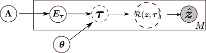
Figure 1: Probabilistic graphical model of the proposed model including model parameters ($\bm{\theta}$, $\bm{\Lambda}$), latent variables ($\bm{E}_{\tau}$) and observables $\hat{\bm{z}}$ from $M$ flow scenaria. Deterministic nodes are indicated with circles with dashed line, stochastic with circles with solid line and known/observed are shaded.

2.2.4 Inference and Learning

On the basis of the probabilistic model proposed and the posterior formulated in the previous section, we discuss numerical inference strategies for identifying the unknown parameters and latent variables. The intractability of the posterior stems from the likelihood which entails the solution of the discretized RANS equations. We advocate the use of Stochastic Variational Inference (SVI) Hoffman et al. (2013) which results in a closed-form approximation of the posterior $p(\bm{\theta},\bm{E}_{\tau}^{(1:M)},\bm{\Lambda}|\mathcal{D})$. In contrast to the popular, sampling-based strategies (MCMC, SMC etc.), SVI yields biased estimates at the benefit of computational efficiency. Given a family of probability densities $q_{\bm{\xi}}\left(\bm{\theta},\bm{\Lambda},\bm{E}_{\tau}^{(1:M)}\right)$ parametrized by $\bm{\xi}$, we find the optimal, i.e. the one that is closest to the exact posterior in terms of their Kullback-Leibler divergence, by maximizing the Evidence Lower Bound (ELBO) $\mathcal{F}(\bm{\xi})$ Bishop and Nasrabadi (2006):

$$\mathcal{F}(\bm{\xi}) =\mathbb{E}_{q_{\xi}\left(\bm{\theta},\bm{\Lambda},\bm{E}_{\tau}^{(1:M)}\right)}\left[\log\left(\frac{p\left(\mathcal{D},\bm{\theta},\bm{\Lambda},\bm{E}_{\tau}^{(1:M)}\right)}{q_{\xi}\left(\bm{\theta},\bm{\Lambda},\bm{E}_{\tau}^{(1:M)}\right)}\right)\right]$$

$$=\mathbb{E}_{q_{\xi}\left(\bm{\theta},\bm{\Lambda},\bm{E}_{\tau}^{(1:M)}\right)}\left[\log\left(\frac{p(\mathcal{D}~{}|~{}\bm{\theta},\bm{E}_{\tau}^{(1:M)})~{}p(\bm{E}_{\tau}^{(1:M)}|\bm{\Lambda})~{}p(\bm{\theta})~{}p(\bm{\Lambda})}{q_{\xi}\left(\bm{\theta},\bm{\Lambda},\bm{E}_{\tau}^{(1:M)}\right)}\right)\right]$$ (24)

As its name suggests, it can be readily shown that ELBO lower-bounds the model log-evidence and their difference is given by the aforementioned KL-divergence i.e.:

$$\log p(\mathcal{D})=\mathcal{F}(\bm{\xi})+KL\left(q_{\xi}(\bm{\theta},\bm{\Lambda},\bm{E}_{\tau}^{(1:M)})~{}\middle|\middle|~{}p(\bm{\theta},\bm{\Lambda},\bm{E}_{\tau}^{(1:M)}|\mathcal{D})\right)$$ (25)

In order to expedite computations we employ a mean-field assumption Blei et al. (2017) according to which the approximate posterior is factorized as:

$$q_{\bm{\xi}}\left(\bm{\theta},\bm{\Lambda},\bm{E}_{\tau}^{(1:M)}\right)=q_{\bm{\xi}}(\bm{\theta})q_{\bm{\xi}}(\bm{\Lambda})\prod_{m=1}^{M}q_{\bm{\xi}}\left(\bm{E}_{\tau}^{(m)}\right).$$ (26)

We employ Dirac-deltas for the first two densities i.e.:

$$q_{\bm{\xi}}(\bm{\theta})=\delta(\bm{\theta}-\bm{\theta}_{MAP})$$ (27)

$$q_{\bm{\xi}}(\bm{\Lambda})=\delta(\bm{\Lambda}-\bm{\Lambda}_{MAP})$$ (28)

In essence, we obtain point estimates for $\bm{\theta},\bm{\Lambda}$ which coincide with the Maximum-A-Posteriori (MAP) estimates. For the model discrepancy variables $\bm{E}_{\tau}^{(m)}$, we employ diagonal Gaussians given by:

$$q_{\bm{\xi}}(\bm{E}_{\tau}^{(m)})=\mathcal{N}(\bm{E}_{\tau}^{(m)}\mid\bm{\mu}^{(m)}_{E},\text{diag}(\bm{\sigma}^{2,(m)}_{E})),\quad\forall i\in\{1,\ldots,M\}$$ (29)

In summary, the vector $\bm{\xi}$ of the parameters in the variational approximation consists of:

$$\bm{\xi}=\{\bm{\theta}_{MAP},\bm{\Lambda}_{MAP},\{\bm{\mu}^{(m)}_{E},\bm{\sigma}^{2,(m)}_{E}\}_{m=1}^{M}\}$$ (30)

The updates of the parameters $\bm{\xi}$ are carried out using derivatives of the ELBO. These entail expectations with respect to $q_{\bm{\xi}}$ which are estimated (with noise) by Monte Carlo in conjunction with the ADAM stochastic optimization scheme Kingma and Ba (2014). In order to reduce the Monte-Carlo noise in the estimates, we employ the reparametrization trick Kingma and Welling (2013). This is made possible here for two reasons: Firstly due to the form of the approximate posterior $q_{\bm{\xi}}$. In particular, if we summarily denote with $\bm{\eta}=\{\bm{\theta},\bm{\Lambda},\bm{E}_{\tau}^{(1:M)}\}$ and given that the approximate posterior $q_{\bm{\xi}}(\bm{\eta})$ can be represented by deterministic transform $\bm{\eta}=g_{\xi}(\bm{\phi})$, where $\bm{\phi}$ follows a known density $q(\bm{\phi})$, the expectations involved in the ELBO and, more importantly, in its gradient can be rewritten as:

$$\nabla_{\bm{\xi}}\mathcal{F}(\bm{\xi}) =\mathbb{E}_{q(\bm{\phi})}\left[\nabla_{\bm{\xi}}g_{\xi}(\bm{\phi})\nabla_{\bm{\eta}}\left(\log p(\mathcal{D},\bm{\eta})-\log q_{\xi}(\bm{\eta})\right)\right]$$ (31)

One observes that derivatives of the log-likelihood with respect to $\bm{\eta}$ are needed. This in turn would imply derivatives of the RANS-model outputs with respect to $\{\bm{\theta},\bm{\Lambda},\bm{E}_{\tau}^{(1:M)}\}$ which appear indirectly through $\bm{\tau}$. Such derivatives are rendered possible by using an adjoint formulation of the discretized RANS model that yields in effect a differentiable solver.

Further details about the derivatives of the ELBO and the use of RANS-model sensitivities obtained by an adjoint formulation can be found in B.

An algorithmic summary of the steps entailed is contained in Algorithm 1.

Input : $\mathcal{D}=\{\hat{\bm{z}}^{(i)}\}_{m=1}^{M}$, $\bm{W}$

Output : $\bm{\xi}=\{\bm{\theta}_{MAP},\bm{\Lambda}_{MAP},\{\bm{\mu}^{(m)}_{E},\bm{\sigma}^{2,(m)}_{E}\}_{m=1}^{M}\}$

while ELBO $\hat{\mathcal{F}}$ not converged do

       $\bm{\theta}\leftarrow\bm{\theta}_{MAP}$,    $\bm{\Lambda}\leftarrow\bm{\Lambda}_{MAP}$ ;

       for $m\in\{1:M\}$ do

             for $k\in\{1:K\}$ do

                   // Reparametrization trick

                   Sample $\bm{\phi}^{(m,k)}\sim\mathcal{N}(~{}\bm{0,~{}I})$ for $k=1,\cdots,K$ ;

                   // Compute stochastic discrepancy terms

                   $\bm{E}_{\tau}^{(m,k)}=g_{\bm{\xi}}(\bm{\phi}^{(m,k)})=\bm{\mu}^{(m)}_{E}+\bm{\sigma}^{(m)}_{E}\odot\bm{\phi}^{(m,k)}$ ;

                   // Solve discretized RANS equations

                   Solve $\mathcal{R}(\bm{z};\bm{\tau}_{\bm{\theta}}(\bm{u})+\bm{W}\bm{E}_{\tau}^{(m,k)})=0$ to obtain the solution vector $\bm{z}^{(m,k)}$ ;

                    // Equation (12)

                   // Compute log-likelihoods and their gradients

                   $\ell^{(m,k)}(\bm{\theta},\bm{E}_{\tau}^{(m,k)}),~{}\partial\ell^{(m,k)}/\partial\bm{\theta},~{}\partial\ell^{(m,k)}/\partial\bm{E}_{\tau}^{(m,k)}$ ;

                    // Equations (36), (41), (42)

                  

             end for

            

       end for

      

      // Monte Carlo estimate of ELBO

       Estimate ELBO $\mathcal{\hat{F}}$ using Equation (43) ;

       // Monte Carlo estimate of the gradient of the ELBO

       Estimate gradient of ELBO $\hat{\nabla_{\bm{\xi}}\mathcal{F}}$ using Equation (45) ;

       // Stochastic Gradient Ascent

       $\bm{\xi}^{(n+1)}\leftarrow\bm{\xi}^{(n)}+\bm{\rho}^{(n)}\odot\hat{\nabla_{\bm{\xi}}\mathcal{F}}$ ;

       $n\leftarrow n+1$ ;

      

end while

return $\bm{\xi}$

Algorithm 1 Inference and Learning using SVI

2.2.5 Predictions

In this section, we describe how probabilistic, predictive estimates of any quantity of interest related to the RANS-simulated flow can be produced using the trained model. In particular, one can obtain a predictive, posterior density $p(\mathbf{z}|\mathcal{D})$ on the whole solution vector $\mathbf{z}$ of the RANS equations as follows:

$$\begin{array}[]{ll}p(\mathbf{z}|\mathcal{D})&=\int p(\mathbf{z},\bm{E}_{\tau},\bm{\theta},\bm{\Lambda}|\mathcal{D})~{}d\bm{E}_{\tau}~{}d\bm{\theta}~{}d\bm{\Lambda}\\ &=\int p(\mathbf{z}|\bm{E}_{\tau},\bm{\theta})~{}p(\bm{E}_{\tau},\bm{\theta},\bm{\Lambda}|\mathcal{D})~{}d\bm{E}_{\tau}~{}d\bm{\theta}~{}d\bm{\Lambda}\\ &=\int p(\mathbf{z}|\bm{E}_{\tau},\bm{\theta})~{}p(\bm{E}_{\tau}|\bm{\Lambda})p(\bm{\theta},\bm{\Lambda}|\mathcal{D})~{}d\bm{E}_{\tau}~{}d\bm{\theta}~{}d\bm{\Lambda}\\ \end{array}$$ (32)

The third of the densities in the intergrand is the posterior which is substituted by its variational approximation i.e. $q_{\bm{\xi}}$ in Equation (26) and for the optimal parameter values $\bm{\xi}$ identified as described in the previous section. The second of the densities represents the prior model prescribed in Equation (20). Finally the first of the densities is simply a Dirac-delta that corresponds to the solution of the RANS equations obtained when using a closure model of the form $\bm{\tau}=\tau_{\bm{\theta}}(\bm{u})+\bm{W}\bm{E}_{\tau}$. In practical terms and given the intractability of this integral, the equation above suggests a Monte Carlo scheme for obtaining samples from $p(\bm{z}|\bm{D})$ which involves the following steps. For each sample:

• Set $\bm{\theta}=\bm{\theta}_{MAP}$, $\bm{\Lambda}=\bm{\Lambda}_{MAP}$. (If a different variational approximation to the posterior $q_{\bm{\xi}}$ than the one in Equations (27), (28) were used, then $\bm{\theta},\bm{\Lambda}$ would need to be sampled from it).

• Sample $\bm{E}_{\tau}$ from $p(\bm{E}_{\tau}|\bm{\Lambda}_{MAP})$ in Equation (20) and compute model discrepancy vector $\bm{\epsilon}_{\tau}=\bm{W}\bm{E}_{\tau}$.

• Solve the discretized RANS model in Equation (12) for $\bm{\tau}=\bm{\tau}_{\bm{\theta}}(\bm{u})+\bm{\epsilon}_{\tau}$.

The aforementioned steps would need to be repeated for as many samples as desired. Subsequently the samples can be used to compute statistics of the predictive estimate (e.g. predictive mean, variance, credible intervals etc) not only of $\mathbf{z}$ (i.e. velocities/pressures) but of any quantity of interest such as the lift, drag, skin friction etc. We note however that stochastic RS discrepancy terms $\bm{\epsilon}_{\tau}$ or $\bm{E}_{\tau}$ and the associated probabilistic model, are limited to the flow geometry used for the training. While it can be used for unseen flow scenarios (e.g. different $Re$ number, inlet conditions, boundary conditions), it cannot be employed to a different flow geometry. In theory, the parametrization of the $\bm{\epsilon}_{\tau}$ can be updated to accommodate different geometries, but we leave it for future investigations. Finally, we would like to highlight the fact that baseline RANS data is not needed as an input to the neural networks for prediction in the proposed scheme, as opposed to other frameworks that have been employed in the past (e.g. Geneva and Zabaras (2019); Ling et al. (2016b); Kaandorp and Dwight (2020); Wang et al. (2017b)).

In terms of computational aspects, the stochastic nature of the (reduced) discrepancy tensor $\bm{E}_{\tau}$ can potentially introduce non-smoothness in the RS vector $\bm{\tau}$ used for solving the RANS equations. In the present work, we have used diagonal covariance for the hyper-prior of $\bm{E}_{\tau}$ given by $\bm{\Lambda}=diag(\bm{\Lambda}^{(J)}),~{}~{}J=1,\ldots,N_{d}$, thus assuming there is no correlation among the nearby nodes/region. As an avenue for future work, a banded covariance matrix can be employed to capture such spatial correlations. Sparsity-inducing priors that account for spatial correlations have been proposed in Bardsley (2013); Wu et al. (2014). Numerical results, training data and the corresponding source code will be made available at https://github.com/pkmtum/D3C-UQ/ upon publication.

3 Numerical Illustrations

3.1 Test case: Backward Facing step

We select the backward facing step configuration in order to assess the proposed modeling framework. This is a classic benchmark problem that has been widely used for studying the performance of turbulence models as it poses significant challenges due to the complex flow features such as flow separation, reattachment and recirculation Nadge and Govardhan (2014); Pioch et al. (2023). In this setup, as illustrated in Fig. (2) a two-dimensional channel flow is abruptly expanded into a rectangular cavity with a step change in height. The flow separates at the step and forms two recirculation zones downstream, one directly after the step and the other on the upper channel wall downstream. These two recirculation zones affect the reattachment length. The flow features can be seen in more detail as depicted in the LES simulations in Fig. (4). In this setting, the Reynolds number is defined as:

$$Re=\frac{uh}{\nu}$$ (33)

where $h$ and $\nu$ are the characteristic length (also the step height) and kinematic viscosity, respectively and $u$ denotes the average velocity of the inlet flow. In the present study, the expansion ratio $H/h$ is 2 and the boundary conditions are shown in Fig. (2). They consist of constant inlet bulk velocity $u_{b}=1$ in the $x$-direction $(u_{b}=u)$ on the left boundary, no-slip condition on $\Gamma_{D}$ (i.e, top/bottom boundary) and zero tractions along $\Gamma_{N}$ (i.e, at the outflow boundary) i.e. $\left(-p\bm{I}+\frac{\nu}{2}(\nabla\bm{u}+\nabla\bm{u}^{T})\right)\cdot\hat{n}=0$ where $\hat{n}$ is the outward normal of the outflow. On the $x-y$ plane, we place the origin at the corner of the step.

Figure 2: Backward facing step flow configuration with step height $h$ and the total channel height $H$. The origin of the $x-y$ plane is placed at the corner of the step. The axes are depicted at the bottom left to avoid clutter.

3.2 Training data generation

In order to generate the training data, we performed Large Eddy Simulations (LES) for various Reynolds numbers i.e. by varying the kinematic viscosity $\nu$. A three-dimensional configuration is adopted wherein the $z$-direction (i.e, the in-plane direction) is periodic and the mean fields averaged over the $z$-direction are used for training. We also performed RANS simulations using the $k-\epsilon$ model for the same set of $Re$ numbers to provide a comparison as it is the most widely used RANS model in industrial applications. In the subsequent discussions, we will refer to the $k-\epsilon$ model as the baseline RANS model.

We used the open-source CFD platform OpenFOAM Jasak et al. (2007) for the LES and baseline RANS simulations. We utilized the steady-state, incompressible solver simpleFoam for the baseline RANS simulations. This solver uses the Semi-Implicit Method for Pressure Linked Equations (SIMPLE) in order to solve both the momentum and pressure equations. For the LES simulations, we employed the pimpleFoam transient solver, which combines both the PISO (Pressure Implicit with Split Operator) and SIMPLE algorithms to solve the pressure and momentum equations. In particular, we use the WALE (Wall-Adapting Local Eddy-Viscosity) model Nicoud and Ducros (1999). This model is well-suited for capturing the turbulent structures near solid walls and is known for its accurate predictions of wall-bounded turbulent flows. We discretized both the baseline RANS and LES domains using second-order methods and all the meshes were non-uniform with mesh density increasing in the domains of interest. To ensure numerical accuracy, we ran all simulations with a CFL number below 0.3. Other pertinent details of the LES and baseline simulations are provided in Table 2.

A few snapshots of the instantaneous velocity magnitude for $Re=1100$ from the LES simulation are depicted in Fig. (3), where one can observe how the flow features of interest evolve over time. Only the time-averaged velocities/pressures were used for training which are shown in Fig. (4). The mean field reference data from LES is interpolated to the same mesh used for the Finite Element (FE)-based calibrated RANS model (model implementation details discussed in the sequel). However, not all the observations in the grid were used for training. The density of observations was higher in the regions of steeper velocity gradients (in the reattachment and recirculation regions) and lower in other regions. In the subsequent results, mean velocity/pressure observations at approximately $8\%$ of the grid points of the RANS-FE mesh were used, i.e. a rather sparse dataset (some indicative observation points are depicted in Figure 10). The influence of the number of observation points on the learning and predictive results is an interesting research direction, which we will be addressed in future investigations.

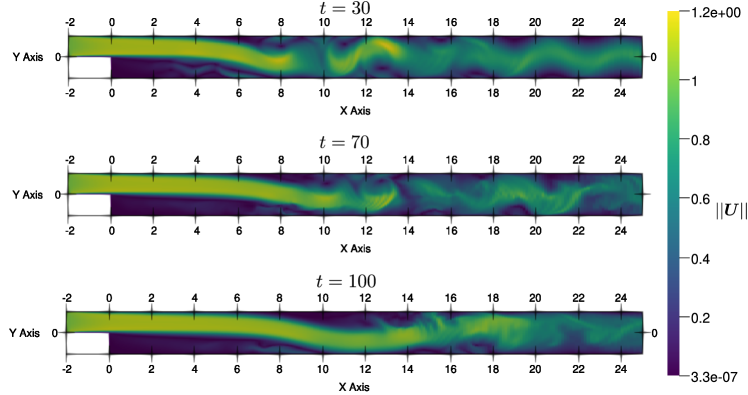
Figure 3: Instantaneous velocity magnitude $||\bm{U}||$ at different time-instants $t=\{30,70,100\}$ obtained from the LES simulation performed at $Re=1100$. We note that the flow eventually reaches a stationary state.

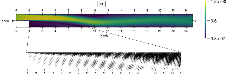
Figure 4: Time-averaged velocity magnitude $||\bm{u}||$ obtained from LES simulation performed at $Re=1100$. The velocity vector plot highlights the flow separation, recirculation zones and the flow reattachment.

Domain Size	$27h\times 2h\times h$
DoF LES	1428920
DoF $k-\epsilon$	35709
step height ($h$)	1
Total channel height ($H$)	2
kinematic viscosity $\nu$ values for training data generation ($\times 10^{-3}$)	$3.33,~{}2.00,~{}1.42,~{}1.11,~{}0.909$
$Re$ values for training data generation	$300,700,900,1100$
$Re$ value for prediction	$500$
characteristic length	step height $h$

Table 2: Parameters used for performing the CFD simulations for the generation of the training and test data Gresho et al. (1993)

3.3 Differentiable forward RANS solver and probabilistic learning implementation

For the discretization of the RANS equations (Equation (12)) the Finite Element (FE) method was employed and the implementation was carried out in the open source package FEniCS Alnæs et al. (2015) due to its innate adjoint solver Mitusch et al. (2019). The basic quantities and their dimensions are listed in Table 3. Further details about the differentiable solver can be found in A.

Probabilistic inference and learning tasks were performed using the probabilistic programming package Pyro Bingham et al. (2019) which is built on top of the popular machine learning library PyTorch Paszke et al. (2019). The ELBO maximization was performed using the ADAM scheme Kingma and Ba (2014). The number of Monte Carlo samples used at each iteration for the estimation of the ELBO and its gradient was $K=5$ (Algorithm 1). The gradient computation of the ELBO (Equation (31)) was enabled by overloading the autograd functionality of PyTorch to facilitate interaction between the solver’s adjoint formulation and the auto-differentiation-based neural network gradient. A relatively small learning rate of $10^{-6}$ was employed due to the Monte Carlo noise in the ELBO gradients. The neural network architecture employed for the parametric RS model was identical to the one suggested by Ling et al. (2016b) where the optimal number of hidden layers and nodes per layer was determined to be 8 and 30 respectively. The Leaky ReLU was chosen as the activation function for all layers. We noted however that the usual practice of random weight initialization was unsuitable as it led to divergence of the solution even after applying the stabilization schemes. For this reason, we used baseline RANS closure data with added noise to pre-train the neural network in order to provide a suitable initialization.

Quantity	dimensions
Domain Size	$27h\times 2h$
number of nodes in FE simulation ($N$)	12180
dim($\bm{z}$)	12180 $\times$ 3
dim($\bm{\tau}$)	12180 $\times$ 3
Boolean Matrix dim($\bm{W}$)	12180 $\times$ 52
dim($\bm{E}$)	52 $\times$ 3
dim($\bm{\Lambda}$)	52 $\times$ 3
dim($\bm{\theta}$)	6970

Table 3: Basic quantities and dimensions

3.4 Results and Discussion

We assessed the trained model for the test-case with $Re=500$ which was not contained in the training data. In the sequel, various aspects of the probabilistic predictions obtained as described in Section (2.2.5) are compared with the reference LES and the baseline RANS predictions. Even though the same parametrized RS closure term was used in Ling et al. (2016b) (and other subsequent works branching from this), their results are not directly comparable due to the use of blending functions Kaandorp and Dwight (2020); Geneva and Zabaras (2019), which combine baseline RS values near the walls with the constant, predicted RS in the bulk and with the amount of blending being case-dependent.

Figure 5: Comparison of the predicted components of the RS tensor $\bm{\tau}_{\bm{\theta}}$ with the LES reference values and the baseline RANS ($k-\epsilon$) for the test case with $Re=500$. The three components $\bm{\tau}_{11}$, $\bm{\tau}_{12}$ and $\bm{\tau}_{22}$ are separately compared in three different blocks. In each block, top - the LES RS tensor component contour, second - the $k-\epsilon$ RS tensor component contour, third - the predicted, parametric RS tensor $\bm{\tau}_{\bm{\theta}}$ for $\bm{\theta}=\bm{\theta}_{MAP}$, fourth - the contour plot of the absolute error between the LES RS tensor and the $\bm{\tau}_{\bm{\theta}}$ tensor component, bottom - the inferred hyper-parameter $\bm{\Lambda}$ of the (reduced) discrepancy tensor $\bm{E_{\tau}}$.

The performance of the proposed method in predicting the components of the RS tensor is shown in Fig. (5), from which the following conclusions can be drawn:

• Even though no RS observations were provided during the training, the parametric $\bm{\tau}_{\bm{\theta}}$ (i.e. neural-network based) part of the RS closure is able to capture the basic features of the reference (i.e. LES) RS field. In contrast, the baseline $k-\epsilon$ model severely under/over-estimates its magnitude and misrepresents its spatial variability.

• The bottom row of all the three blocks in Fig. (5) depicts the inferred precision $\bm{\Lambda}$ of the (reduced) discrepancy tensor $\bm{E}_{\tau}$. As this is inversely proportional to the predictive uncertainty, we note that it attains smaller values in the regions where the parametric model $\bm{\tau}_{\bm{\theta}}$ deviates the most from the LES values (e.g. for $5<x/h<10$). Conversely, it attains very large values (which correspond to practically zero model discrepancies) in areas where the parametric closure model is able to correctly account for the underlying phenomena (e.g. far downstream and for all three RS components). This is expected as the flow attains an almost parabolic profile in this region, which in turn translates to reduced fluctuations in the RS tensor, making it easier for the neural network to learn.

The Monte-Carlo-based scheme (detailed in Section (2.2.5)) was employed to propagate the model form uncertainty forward in order to obtain probabilistic predictive estimates for the quantities of interest i.e. mean stream-wise velocity $u$, wall-normal velocity $v$ (Fig. (6), Fig. (7)) and mean pressure $p$ (Fig. (8)). Cross-sections of the aforementioned quantities are depicted in Fig. (9). The following conclusions can be drawn from the Figures:

• Even though the RS field is captured with some discrepancies, the predicted mean fields agree well with the reference LES data (Figures 6, 7 and 8, discussed in the sequel). This points to the non-uniqueness of this inverse problem solution, also reported by other works Duraisamy (2021); Brenner et al. (2022).

• There exist two recirculation zones in the backward-facing step flow setup. The primary one forms just after the step and the secondary appears above it for Reynolds numbers close to 400 and above, for the given expansion ratio Armaly et al. (1983). As it can be seen in Fig. (6), the proposed model is able to predict the appearance of the two recirculation zones in close agreement with the LES, whereas the baseline RANS model underestimates the size of the first recirculation zone and almost completely misses the second one.

• The last row of Fig. (6) depicts the predictive posterior standard deviation of the aforementioned quantities. As expected, around the shear layers (the top of the first recirculation zone and the bottom of the second recirculation zone), the uncertainty is the highest. This is even more clearly observed in the cross-sections of Fig. (9) which illustrate the predictive, posterior mean plus/minus two posterior standard deviations. More importantly perhaps, one observes that the predictions envelop the reference LES values in most areas. The model is extremely confident close to the inlet, as manifested by the very tight credible interval. As one moves further downstream and close to the first recirculation zone, the parametric closure suffers, hence the uncertainty bounds are wider to account for it. The ability to quantify aleatoric, predictive uncertainty is one of the main advantages of the probabilistic model proposed in contrast to the more commonly used deterministic counterparts as well as alternatives that can only capture epistemic uncertainty.

• Similarly to the stream-wise velocity, predictions for the wall-normal velocity (Fig. (7)) and the pressure (Fig. (8)) are in good agreement with the reference LES values, as opposed to the baseline RANS. In the first recirculation zone, the baseline $k-\epsilon$ is completely off, while the predicted values with the credible interval covers the reference LES. Also, the pressure predictions (Fig. (8)) identify the crucial zone where the flow reattaches to the wall (around $x/h\approx 10$), which is very difficult to predict in general. At the reattachment point, there is a transition from low-pressure in the recirculation zone to higher pressure along the wall. The posterior standard deviation at this point is also higher than in the other regions, ensuring that the reference solution is enveloped.

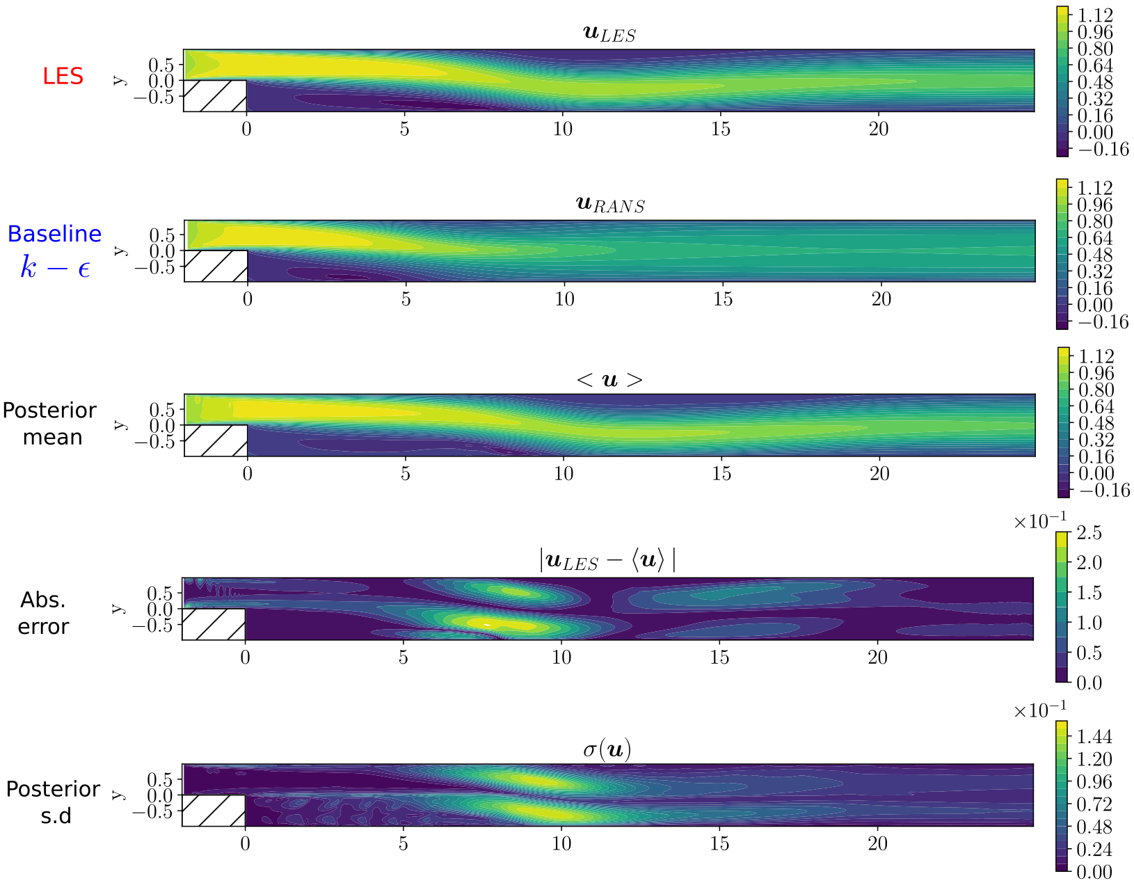
Figure 6: Velocity contours in x-direction ($\bm{u}$) for the test case with Re = 500. top - ground truth (LES), second - baseline $k-\epsilon$, third - the posterior predictive mean ($\left<\bm{u}\right>$), fourth - the contour plot of the absolute error between the LES ($\bm{u}_{LES}$) and the posterior predictive mean ($\left<\bm{u}\right>$), bottom - the standard deviation of the posterior predictive ($\sigma(\bm{u})$)

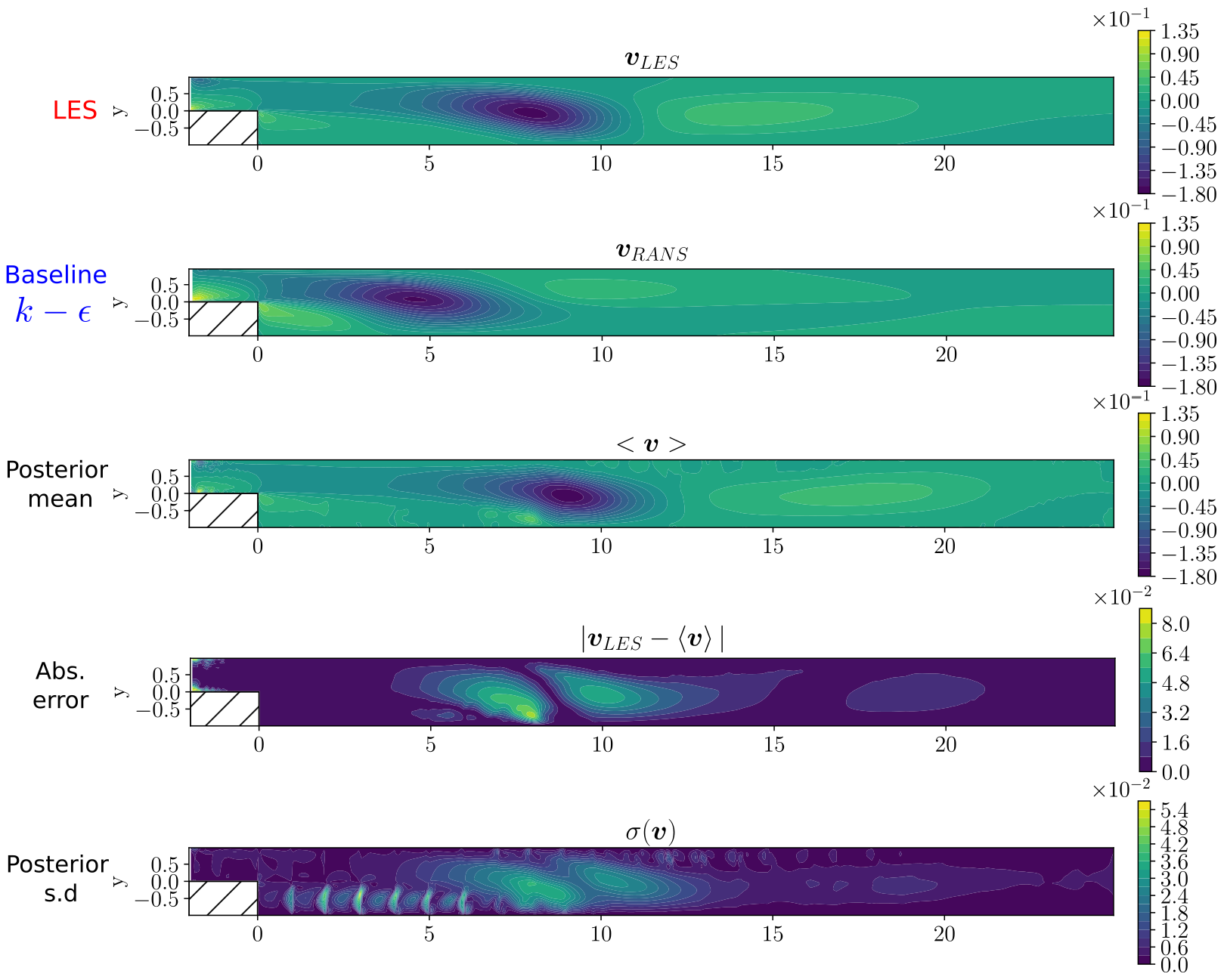
Figure 7: Velocity contours in y-direction ($\bm{v}$) for the test case with Re = 500. top - ground truth (LES), second - baseline $k-\epsilon$, third - the posterior predictive mean ($\left<\bm{v}\right>$), fourth - the contour plot of the absolute error between the LES ($\bm{v}_{LES}$) and the posterior predictive mean ($\left<\bm{v}\right>$), bottom - the standard deviation of the posterior predictive ($\sigma(\bm{v})$).

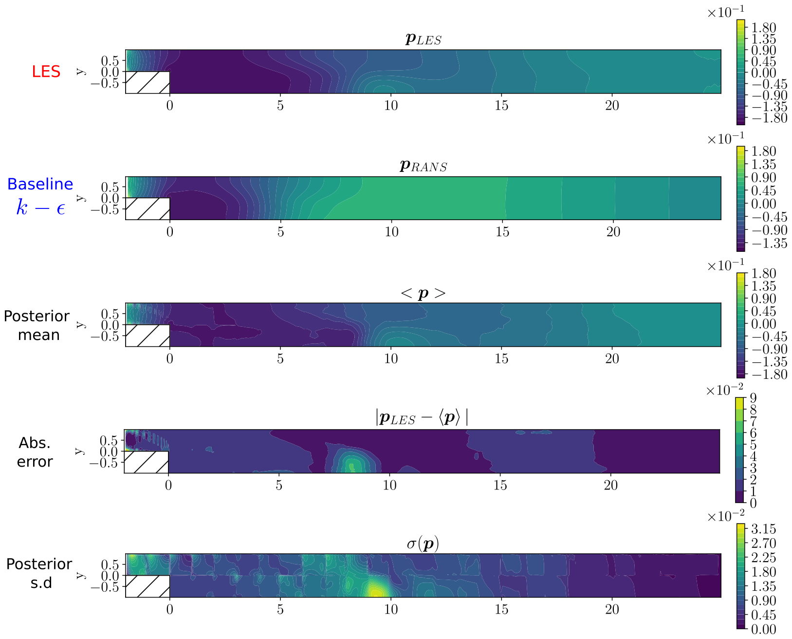
Figure 8: Pressure contours ($\bm{p}$) for the test case with Re = 500. top - ground truth (LES), second - baseline $k-\epsilon$, third - the posterior predictive mean ($\left<\bm{u}\right>$), fourth - the contour plot of the absolute error between the LES ($\bm{p}_{LES}$) and the posterior predictive mean ($\left<\bm{p}\right>$), bottom - the standard deviation of the posterior predictive ($\sigma(\bm{u})$)

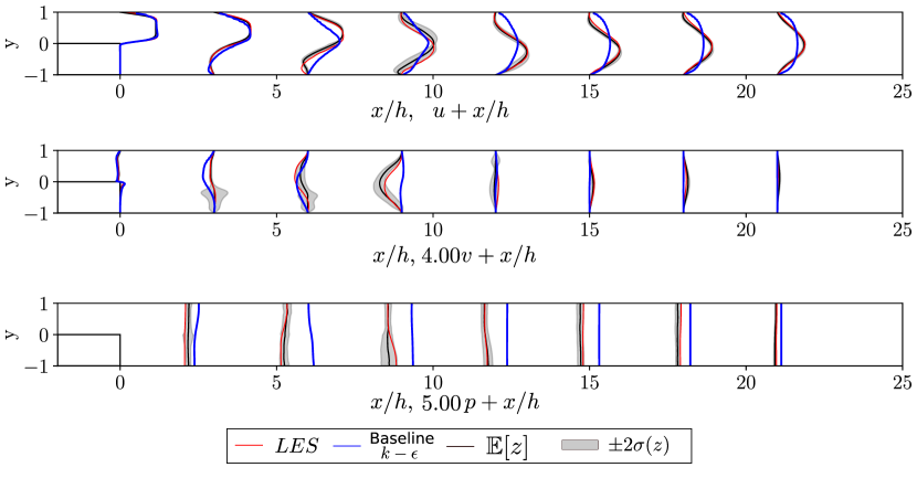
Figure 9: Section plots at different locations $x/h$ comparing the LES and Baseline RANS mean fields with the posterior predictive mean (solid black line) and $\pm 2\times$ standard deviation (shaded area) for the test case with Re = 500. top - velocity in x-direction ($\bm{u}$), middle - velocity in the y-direction ($\bm{v}$), bottom - pressure ($\bm{p}$). $\mathbb{E}[z]$ and $\sigma(z)$ depict the predictive posterior mean and standard deviation respectively.

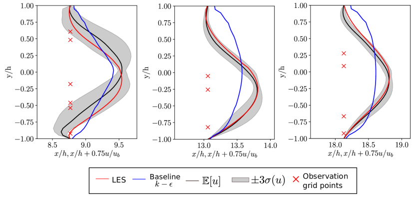
Figure 10: Section plots of the stream-wise velocity ${u}$ at three different $x/h$ locations for the test case with $Re=500$. In addition, the points where training observations were available are depicted with red crosses. $\mathbb{E}[u]$ and $\sigma(u)$ depict the predictive posterior mean and standard deviation respectively.

As previously mentioned, observations of mean velocities/pressures at approximately $8\%$ of the total number of grid points in the FE mesh were used for training. Fig. (10) highlights this by comparing the stream-wise velocity at three different sections $x/h$. The left subfigure depicts the section in the first re-circulation zone. It can be seen that despite having very few observation points near the wall, the $u$ predictions are able to capture the backward flow in the re-circulation regions. In contrast, the baseline $k-\epsilon$ completely fails to capture it. This can be attributed to the earlier reattachment of the flow in the baseline $k-\epsilon$ case (flow reattachment discussed in the sequel). The middle and the right subfigures depict sections further downstream, with the middle being in the second re-circulation zone and the right in the flow recovery zone. It is observed that with a relatively small number of observation points, the trained model’s prediction is in agreement with the LES. Furthermore the latter is enveloped by the credible interval constructed by considering $\pm 3\times$ (the posterior standard deviation). This credible interval is much tighter as compared to the one in the left subfigure.

Accurately capturing the recirculation zones is crucial to getting a reliable estimate of the reattachment length, which is a key parameter in the study of separated flows, such as the case here. The reattachment length is defined as the distance from the step where the flow separates to the point at which it reattaches to the surface downstream of the step. Reattachment occurs where the velocity gradient off the wall is zero, or in other words, where the wall shear stress is zero. The predicted reattachment length ($x_{reattach}$) by the proposed method is compared with a) the LES data (Section (3.2)) b) the baseline RANS (Section (3.2)) c) the two-dimensional, LES simulation performed by Biswas et al. (2004) for the expansion ratio of $1.9423$, and d) the results in Geneva and Zabaras (2019), who used the same Tensor Basis Neural Networks (TBNN) Ling et al. (2016b) employed in the parametric closure term in our work as well. The results are summarized in Table 4 where it is evident that while previous works deviated significantly from the reference LES value, our probabilistic prediction is able to envelop it.

The reattachment length is heavily dependent on correctly identifying the two recirculation zones and the baseline RANS model fails to predict the secondary recirculation zone (Fig. (6)). This might have resulted in such a low reattachment length. The estimate of the reattachment length is also low in Geneva and Zabaras (2019), which could be attributed to the lack of the stochastic, model correction term.

Model	$x_{reattach}$[x/h]
LES (reference)	9.10
Biswas et al. Biswas et al. (2004) ($H/h=1.9423$)	8.9
Baseline RANS ($k-\epsilon$ model)	5.61
Geneva et al.Geneva and Zabaras (2019)	5.52
proposed model	10.06 $\pm$ 1.21

Table 4: Predictions of reattachment length ($x/h$) of the primary recirculation region behind the backward-facing step (expansion ratio $H/h=2$) for the test case with $Re=500$. The $\pm$ corresponds to $3\times$ the posterior standard deviation.

4 Conclusions

We have presented a data-driven model for RANS simulations that quantifies and propagates in its predictions an often neglected source of uncertainty, namely the aleatoric, model uncertainty in the closure equations. We have combined this with a parametric closure model which employs a set of tensor basis functions that depend on the invariants of the rate of strain and rotation tensors. A fully Bayesian formulation is advocated which makes use of a sparsity-inducing prior in order to identify the regions in the problem domain where the parametric closure is insufficient and in order to quantify the stochastic correction to the Reynolds stress tensor. We have demonstrated how the model can be trained using sparse, indirect data, namely mean velocities/pressures in contrast to the majority of pertinent efforts that require direct, RS data. While the training data in our illustrations arose from a higher-fidelity model, one can readily envision using experimental observations as well.

In order to enable inference and learning tasks, we developed a differentiable RANS solver capable of providing parametric sensitivities. Such a differentiable solver was non-trivial owing to the complexity of the physical simulator and its stability issues. The lack of such numerical tools has proven to be a significant barrier for intrusive, physics-based, data-driven models in turbulence Cranmer et al. (2020). This differentiable solver was utilized in the context of a Stochastic Variational Inference (SVI) scheme that employs Monte Carlo estimates of the ELBO derivatives in conjunction with the reparametrization trick and stochastic gradient ascent. We demonstrated how probabilistic predictive estimates can be computed for all output quantities of the trained RANS model and illustrated their accuracy on a separated flow in the backward facing step benchmark problem. In most cases very good agreement with the reference values was achieved and in all cases these were enveloped by the credible intervals computed.

The proposed modeling framework offers several possibilities for extensions, some of which we discuss below:

• The indirect data i.e. velocities/pressures as in the Equation (22), could be complemented with direct, RS data at certain locations of the problem domain. This could be beneficial in improving the model’s predictive accuracy and generalization capabilities.

• The parametric closure model could benefit from non-local dependencies which could be enabled by convolutional or vector-cloud neural networks (VCNN) Han et al. (2022) with appropriate embedding of invariance properties.

• The dimensionality reduction of the stochastic discrepancy terms (Equation (19)) was based on a pre-selected and uniform division of the problem domain into subdomains. The accuracy of the model would certainly benefit from a learnable and adaptive such scheme that would be able to focus on the areas where model deficiencies are most pronounced and stochastic corrections are most needed.

Appendix A Differentiable RANS solver

In the present study, the RANS equations (Equation (7)) are numerically solved using the finite element discretization, implemented in the open source package FEniCS Alnæs et al. (2015). The discrete equations are obtained by representing the solution and test functions in appropriate finite dimensional function spaces. In particular, we employed the standard Taylor-Hood pair of basis functions with polynomial degree one for the pressure interpolants and two for the velocities. This choice is made to avoid stability issues potentially arising from the interaction between the momentum and continuity equations.

The turbulence scaling terms, $k$ and $\epsilon$ in Equation (17), are obtained by solving the respective standard transport equations Pope (2000); Alfonsi (2009). Symmetry is enforced in the RS tensor, i.e. $\tau_{xy}$ and $\tau_{yx}$ are identical without any redundancy in the representation. The discretized system is solved with damped Newton’s method. For robustness and global convergence, pseudo-time stepping is used with the backward Euler discretization Deuflhard (2005). As the Reynolds number is increased, the convection term dominates, leading to stability Donea and Huerta (2003).This elicits a need to add stabilization terms to the weak form, such as the least-square stabilization, according to which the weighted square of the strong form is added to the weak form residual. However, these extra terms have to be chosen carefully in order not to compromise the correctness of the approximate solution. Classically, researchers added artificial diffusion terms or a numerical diffusion by using upwind scheme for the convection term instead of central diffusion. The extra infused term corrupted the solution quality. To avoid this, in practice, it is common to use schemes like Streamline-Upwind Petrov-Gelarkin method (SUPG) and Galerkin Least Squares (GLS). In the present study, we have utilized a self-adjoint numerical stabilisation scheme which is an extension of Gelarkin Least Squares (GLS) Stabilisation called Galerkin gradient least square method Franca and Do Carmo (1989). This amounts to adding a stabilization term to the residual weak form. For additional details, interested readers are referred to Franca and Do Carmo (1989); Donea and Huerta (2003).

Appendix B Adjoint Formulation and Estimation of the Gradient of the ELBO

As discussed in Section 2.2.4, the SVI framework advocated, in combination with the reparametrization trick, requires derivatives of the ELBO with respect to the variables which we summarily denoted by $\bm{\eta}=\{\bm{\theta},\bm{\Lambda},\bm{E}_{\tau}^{(1:M)}\}$, i.e. (as in Equation (31)):

$$\nabla_{\bm{\xi}}\mathcal{F}(\bm{\xi})=\mathbb{E}_{q(\bm{\phi})}\left[\nabla_{\bm{\xi}}g_{\xi}(\bm{\phi})\nabla_{\bm{\eta}}\left(\log p(\mathcal{D},\bm{\eta})-\log q_{\xi}(\bm{\eta})\right)\right]$$ (34)

where from Equation (23):

$$\begin{array}[]{ll}\log p(\mathcal{D},\bm{\eta})&=\log\left(p(\mathcal{D}~{}|~{}\bm{\theta},\bm{E}_{\tau}^{(1:M)})~{}p(\bm{E}_{\tau}^{(1:M)}|\bm{\Lambda})~{}p(\bm{\theta})~{}p(\bm{\Lambda})\right)\\ &=\left(\sum_{m=1}^{M}\log p(\hat{\bm{z}}^{(m)}\mid\bm{\theta},\bm{E}_{\tau}^{(m)})+\log p(\bm{E}_{\tau}^{(m)}|\bm{\Lambda})\right)~{}+\log p(\bm{\theta})+\log~{}p(\bm{\Lambda})\end{array}$$ (35)

The form of the (log-)priors $p(\bm{E}_{\tau}^{(m)}|\bm{\Lambda})$ (Equation (20)), $p(\bm{\theta})$ (Equation (18)), $p(\bm{\Lambda})$ (Equation (21)) as well as of the approximate posterior $q_{\xi}(\bm{\eta})$ (Equations (26) and (27), (28), (29)) suggest that most of these derivatives can be analytically computed with the exception of the ones involving the log-likelihoods, i.e.:

$$\ell^{(m)}(\bm{\theta},\bm{E}_{\tau}^{(m)})=\log p(\hat{\bm{z}}^{(m)}\mid\bm{\theta},\bm{E}_{\tau}^{(m)}).$$ (36)

This is because each of these terms depends implicitly on $\bm{\theta},\bm{E}_{\tau}^{(m)}$ through the output of the RANS solver $\bm{z}(\bm{\theta},\bm{\epsilon}_{\tau}^{(m)}=\bm{W}\bm{E}_{\tau}^{(m)})$ with the closure model for the discretized RS tensor field suggested by Equation (13) i.e. $\bm{\tau}=\bm{\tau}_{\bm{\theta}}(\bm{u})+\bm{W}\bm{E}_{\tau}^{(m)}$. In view of the governing equations (Equation (12)), we explain below how adjoint equations can be formulated that enable efficient computation of the aforementioned derivatives of the log-likelihoods.

In particular, and if we drop the superscript $m$ for each term in the log-likelihood in order to simplify the notation, we formulate a Lagrangian with the help of a vector $\lambda$ of Lagrangian multipliers, i.e.:

$$\mathcal{L}=\ell+\bm{\lambda}^{T}(\mathcal{G}(\bm{z})-\bm{B}\bm{\tau})$$ (37)

where $\mathcal{G}$, $\bm{B}$, $\bm{\tau}$ and $\bm{z}$ are as defined in Section (2.2).Differentiating with respect to $\bm{\tau}$ yields:

$$\frac{d\mathcal{L}}{d\bm{\tau}} =\frac{\partial\ell}{\partial\bm{z}}\frac{d\bm{z}}{d\bm{\tau}}+\frac{d\bm{\lambda}^{T}}{d\bm{\tau}}(\mathcal{G}(\bm{z})-\bm{B}\bm{\tau})+\bm{\lambda}^{T}\left(\frac{\partial\mathcal{G}}{\partial\bm{z}}\frac{d\bm{z}}{d\bm{\tau}}-\bm{B}\right)$$

$$=\left(\frac{\partial\ell}{\partial\bm{z}}+\bm{\lambda}^{T}\frac{\partial\mathcal{G}}{\partial\bm{z}}\right)\frac{d\bm{z}}{d\bm{\bm{\tau}}}-\bm{\lambda}^{T}\bm{B}$$ (38)

We select $\bm{\lambda}^{T}$ so that the first term in parentheses vanishes, i.e. :

$$\frac{\partial\ell}{\partial\bm{z}}+\bm{\lambda}^{T}\frac{\partial\mathcal{G}}{\partial\bm{z}}=0\quad\textrm{or,}\quad\left(\frac{\partial\mathcal{G}}{\partial\bm{z}}\right)^{T}\bm{\lambda}=-\left(\frac{\partial\ell}{\partial\bm{z}}\right)^{T}$$ (39)

The linear system of equations was solved using a direct LU solver. The vector $\bm{\lambda}$ found was substituted in Equation (38) in order to obtain the desired gradient which is given by:

$$\frac{d\mathcal{L}}{d\bm{\tau}}=\frac{d\ell}{d\bm{\tau}}=-\bm{\lambda}^{T}\bm{B}$$ (40)

Subsequently, and by application of the chain rule we can obtain derivatives with respect to $\bm{\theta}$ as:

$$\frac{d\ell}{d\bm{\theta}}=\underbrace{\frac{\partial\ell}{\partial\bm{\tau}}}_{\begin{subarray}{c}\text{Adjoint}\\ \text{model}\end{subarray}}\underbrace{\frac{\partial\bm{\tau}}{\partial\bm{\theta}}}_{\begin{subarray}{c}\text{NN}\\ \text{auto-diff}\end{subarray}}$$ (41)

where $\partial\bm{\tau}/\partial\bm{\theta}$ was efficiently computed by back-propagation, which is a reverse accumulation automatic differentiation algorithm for deep neural networks that applies the chain rule on a per-layer basis. We note that since the parameters $\bm{\theta}$ are common for each likelihood $\ell^{(m)}$ the aforementioned terms would need to be added as per Equation (35).

Similarly by chain rule, the gradient with respect to the vector $\bm{E}_{\tau}$ is given by:

$$\frac{d\ell}{d\bm{E}_{\tau}}=\bm{W}^{T}\frac{d\ell}{d\bm{\tau}}$$ (42)

We note finally that the expectations involved in the ELBO and its gradient (Equation (31)) are approximated by Monte Carlo i.e.:

$$\mathcal{F}(\bm{\xi})\approx\frac{1}{K}\left(\sum_{k=1}^{K}\left(\sum_{m=1}^{M}\ell^{(m)}(\bm{\theta},\bm{E}_{\tau}^{(m,k)})+\log p(\bm{E}_{\tau}^{(m,k)}|\bm{\Lambda})\right)~{}+\log p(\bm{\theta})+\log~{}p(\bm{\Lambda})-\log q_{\xi}(\bm{\theta},\bm{\Lambda},\bm{E}_{\tau}^{(m,k)})\right)$$ (43)

where:

$$\bm{\phi}^{(m,k)}\sim\mathcal{N}(\bm{0,I}),~{}~{}\bm{E}_{\tau}^{(m,k)}=g_{\bm{\xi}}(\bm{\phi}^{(m,k)}),$$ (44)

and:

$$\nabla_{\bm{\xi}}\mathcal{F}(\bm{\xi})\approx\frac{1}{K}\sum_{k=1}^{K}\nabla_{\bm{\xi}}g_{\xi}(\bm{\phi}^{(k)})\nabla_{\bm{\eta}}\left(\log p(\mathcal{D},\bm{\eta}^{(k)})-\log q_{\xi}(\bm{\eta}^{(k)})\right)\\$$ (45)

where $\bm{\eta}^{(k)}=g_{\xi}(\bm{\phi}^{(k)})$.

References

- Ahmed et al. (2021) Ahmed, S.E., Pawar, S., San, O., Rasheed, A., Iliescu, T., Noack, B.R., 2021. On closures for reduced order models—A spectrum of first-principle to machine-learned avenues. Physics of Fluids 33. URL: https://doi.org/10.1063/5.0061577, doi:10.1063/5.0061577. 091301.
- Alfonsi (2009) Alfonsi, G., 2009. Reynolds-Averaged Navier-Stokes Equations for Turbulence Modeling. Applied Mechanics Reviews - APPL MECH REV 62. doi:10.1115/1.3124648.
- Alnæs et al. (2015) Alnæs, M., Blechta, J., Hake, J., Johansson, A., Kehlet, B., Logg, A., Richardson, C., Ring, J., Rognes, M.E., Wells, G.N., 2015. The fenics project version 1.5. Archive of Numerical Software 3.
- Armaly et al. (1983) Armaly, B.F., Durst, F., Pereira, J., Schönung, B., 1983. Experimental and theoretical investigation of backward-facing step flow. Journal of fluid Mechanics 127, 473–496.
- Bardsley (2013) Bardsley, J.M., 2013. Gaussian markov random field priors for inverse problems. Inverse Problems and Imaging 7, 397–416. doi:10.3934/ipi.2013.7.397.
- Bezgin et al. (2021) Bezgin, D.A., Buhendwa, A.B., Adams, N.A., 2021. A fully-differentiable compressible high-order computational fluid dynamics solver. arXiv preprint arXiv:2112.04979 .
- Bidar et al. (2022) Bidar, O., He, P., Anderson, S., Qin, N., 2022. An Open-source Adjoint-based Field Inversion Tool for Data-driven RANS Modelling. doi:10.2514/6.2022-4125.
- Bingham et al. (2019) Bingham, E., Chen, J.P., Jankowiak, M., Obermeyer, F., Pradhan, N., Karaletsos, T., Singh, R., Szerlip, P., Horsfall, P., Goodman, N.D., 2019. Pyro: Deep universal probabilistic programming. The Journal of Machine Learning Research 20, 973–978.
- Bishop and Nasrabadi (2006) Bishop, C.M., Nasrabadi, N.M., 2006. Pattern recognition and machine learning. volume 4. Springer.
- Biswas et al. (2004) Biswas, G., Breuer, M., Durst, F., 2004. Backward-facing step flows for various expansion ratios at low and moderate reynolds numbers. J. Fluids Eng. 126, 362–374.
- Blei et al. (2017) Blei, D.M., Kucukelbir, A., McAuliffe, J.D., 2017. Variational inference: A review for statisticians. Journal of the American statistical Association 112, 859–877.
- Brenner et al. (2022) Brenner, O., Piroozmand, P., Jenny, P., 2022. Efficient assimilation of sparse data into rans-based turbulent flow simulations using a discrete adjoint method. Journal of Computational Physics 471, 111667.
- Brunton et al. (2020) Brunton, S.L., Noack, B.R., Koumoutsakos, P., 2020. Machine learning for fluid mechanics. Annual Review of Fluid Mechanics 52, 477–508.
- Brunton et al. (2016) Brunton, S.L., Proctor, J.L., Kutz, J.N., 2016. Discovering governing equations from data by sparse identification of nonlinear dynamical systems. Proceedings of the national academy of sciences 113, 3932–3937. Publisher: National Acad Sciences.
- Cranmer et al. (2020) Cranmer, K., Brehmer, J., Louppe, G., 2020. The frontier of simulation-based inference. Proceedings of the National Academy of Sciences 117, 30055–30062.
- Deuflhard (2005) Deuflhard, P., 2005. Newton methods for nonlinear problems: affine invariance and adaptive algorithms. volume 35. Springer Science & Business Media.
- Donea and Huerta (2003) Donea, J., Huerta, A., 2003. Finite element methods for flow problems. John Wiley & Sons.
- Duraisamy (2021) Duraisamy, K., 2021. Perspectives on Machine Learning-augmented Reynolds-averaged and Large Eddy Simulation Models of Turbulence. Physical Review Fluids 6, 050504. URL: http://arxiv.org/abs/2009.10675, doi:10.1103/PhysRevFluids.6.050504. arXiv:2009.10675 [physics].
- Duraisamy et al. (2019) Duraisamy, K., Iaccarino, G., Xiao, H., 2019. Turbulence modeling in the age of data. Annual Review of Fluid Mechanics 51, 357–377.
- Edeling et al. (2014) Edeling, W.N., Cinnella, P., Dwight, R.P., Bijl, H., 2014. Bayesian estimates of parameter variability in the k– turbulence model. Journal of Computational Physics 258, 73–94.
- Edeling et al. (2018) Edeling, W.N., Iaccarino, G., Cinnella, P., 2018. Data-free and data-driven rans predictions with quantified uncertainty. Flow, Turbulence and Combustion 100, 593–616.
- Emory et al. (2013) Emory, M., Larsson, J., Iaccarino, G., 2013. Modeling of structural uncertainties in reynolds-averaged navier-stokes closures. Physics of Fluids 25, 110822.
- Felsberger and Koutsourelakis (2019) Felsberger, L., Koutsourelakis, P., 2019. Physics-constrained, data-driven discovery of coarse-grained dynamics. Communications in Computational Physics 25, 1259–1301. doi:10.4208/cicp.OA-2018-0174.
- Franca and Do Carmo (1989) Franca, L.P., Do Carmo, E.G.D., 1989. The galerkin gradient least-squares method. Computer Methods in Applied Mechanics and Engineering 74, 41–54.
- Geneva and Zabaras (2019) Geneva, N., Zabaras, N., 2019. Quantifying model form uncertainty in reynolds-averaged turbulence models with bayesian deep neural networks. Journal of Computational Physics 383, 125–147.
- Giles et al. (2003) Giles, M.B., Duta, M.C., Muller, J.D., Pierce, N.A., 2003. Algorithm developments for discrete adjoint methods. AIAA journal 41, 198–205.
- Giles and Pierce (2000) Giles, M.B., Pierce, N.A., 2000. An introduction to the adjoint approach to design. Flow, turbulence and combustion 65, 393–415.
- Gorlé and Iaccarino (2013) Gorlé, C., Iaccarino, G., 2013. A framework for epistemic uncertainty quantification of turbulent scalar flux models for reynolds-averaged navier-stokes simulations. Physics of Fluids 25, 055105.
- Gresho et al. (1993) Gresho, P.M., Gartling, D.K., Torczynski, J., Cliffe, K., Winters, K., Garratt, T., Spence, A., Goodrich, J.W., 1993. Is the steady viscous incompressible two-dimensional flow over a backward-facing step at re= 800 stable? International Journal for Numerical Methods in Fluids 17, 501–541.
- Han et al. (2022) Han, J., Zhou, X.H., Xiao, H., 2022. Vcnn-e: A vector-cloud neural network with equivariance for emulating reynolds stress transport equations. arXiv preprint arXiv:2201.01287 .
- Hoffman et al. (2013) Hoffman, M.D., Blei, D.M., Wang, C., Paisley, J., 2013. Stochastic variational inference. Journal of Machine Learning Research .
- (32) Holland, J.R., Baeder, J.D., Duraisamy, K., . Towards Integrated Field Inversion and Machine Learning With Embedded Neural Networks for RANS Modeling, in: AIAA Scitech 2019 Forum. American Institute of Aeronautics and Astronautics. URL: https://arc.aiaa.org/doi/abs/10.2514/6.2019-1884, doi:10.2514/6.2019-1884. _eprint: https://arc.aiaa.org/doi/pdf/10.2514/6.2019-1884.
- Iaccarino et al. (2017) Iaccarino, G., Mishra, A.A., Ghili, S., 2017. Eigenspace perturbations for uncertainty estimation of single-point turbulence closures. Physical Review Fluids 2. doi:10.1103/PhysRevFluids.2.024605.
- Jameson (1988) Jameson, A., 1988. Aerodynamic design via control theory. Journal of scientific computing 3, 233–260.
- Jasak et al. (2007) Jasak, H., Jemcov, A., Tukovic, Z., et al., 2007. Openfoam: A c++ library for complex physics simulations, in: International workshop on coupled methods in numerical dynamics, pp. 1–20.
- Kaandorp and Dwight (2020) Kaandorp, M.L., Dwight, R.P., 2020. Data-driven modelling of the reynolds stress tensor using random forests with invariance. Computers & Fluids 202, 104497.
- Kingma and Ba (2014) Kingma, D.P., Ba, J., 2014. Adam: A method for stochastic optimization. arXiv preprint arXiv:1412.6980 .
- Kingma and Welling (2013) Kingma, D.P., Welling, M., 2013. Auto-encoding variational bayes. arXiv preprint arXiv:1312.6114 .
- Kochkov (2021) Kochkov, D., 2021. Machine learning–accelerated computationalfluid dynamics .
- Koutsourelakis et al. (2016) Koutsourelakis, P.S., Zabaras, N., Girolami, M., 2016. Big data and predictive computational modeling. Journal of Computational Physics 321, 1252–1254.
- Launder et al. (1975) Launder, B.E., Reece, G.J., Rodi, W., 1975. Progress in the development of a reynolds-stress turbulence closure. Journal of fluid mechanics 68, 537–566.
- Launder and Sharma (1974) Launder, B.E., Sharma, B.I., 1974. Application of the energy-dissipation model of turbulence to the calculation of flow near a spinning disc. Letters in Heat and Mass Transfer 1, 131–137. doi:10.1016/0094-4548(74)90150-7.
- Ling et al. (2016a) Ling, J., Jones, R., Templeton, J., 2016a. Machine learning strategies for systems with invariance properties. Journal of Computational Physics 318, 22–35. URL: http://dx.doi.org/10.1016/j.jcp.2016.05.003, doi:10.1016/j.jcp.2016.05.003. publisher: Elsevier Inc.
- Ling et al. (2016b) Ling, J., Kurzawski, A., Templeton, J., 2016b. Reynolds averaged turbulence modelling using deep neural networks with embedded invariance. Journal of Fluid Mechanics 807, 155–166.
- List et al. (2022) List, B., Chen, L.W., Thuerey, N., 2022. Learned turbulence modelling with differentiable fluid solvers. arXiv preprint arXiv:2202.06988 .
- Lucor et al. (2022) Lucor, D., Agrawal, A., Sergent, A., 2022. Simple computational strategies for more effective physics-informed neural networks modeling of turbulent natural convection. Journal of Computational Physics 456, 111022. URL: https://doi.org/10.1016/j.jcp.2022.111022, doi:10.1016/j.jcp.2022.111022. publisher: Elsevier Inc.
- Marusic and Broomhall (2021) Marusic, I., Broomhall, S., 2021. Leonardo da vinci and fluid mechanics. Annual Review of Fluid Mechanics 53, 1–25. doi:10.1146/annurev-fluid-022620-122816.
- Mishra and Iaccarino (2017) Mishra, A.A., Iaccarino, G., 2017. Uncertainty estimation for reynolds-averaged navier-stokes predictions of high-speed aircraft nozzle jets. AIAA Journal 55, 3999–4004. doi:10.2514/1.J056059.
- Mitusch et al. (2019) Mitusch, S.K., Funke, S.W., Dokken, J.S., 2019. dolfin-adjoint 2018.1: automated adjoints for fenics and firedrake. Journal of Open Source Software 4, 1292.
- Nadge and Govardhan (2014) Nadge, P.M., Govardhan, R., 2014. High reynolds number flow over a backward-facing step: structure of the mean separation bubble. Experiments in fluids 55, 1–22.
- Neal (2012) Neal, R.M., 2012. Bayesian learning for neural networks. volume 118. Springer Science & Business Media.
- Nicoud and Ducros (1999) Nicoud, F., Ducros, F., 1999. Subgrid-scale stress modelling based on the square of the velocity gradient tensor. Flow, turbulence and Combustion 62, 183–200.
- Oliver and Moser (2009) Oliver, T., Moser, R., 2009. Uncertainty quantification for rans turbulence model predictions, in: APS division of fluid dynamics meeting abstracts, pp. LC–004.
- Oliver and Moser (2011) Oliver, T.A., Moser, R.D., 2011. Bayesian uncertainty quantification applied to RANS turbulence models, in: Journal of Physics: Conference Series, Institute of Physics Publishing. p. 042032. URL: https://iopscience.iop.org/article/10.1088/1742-6596/318/4/042032, doi:10.1088/1742-6596/318/4/042032.
- Parish and Duraisamy (2015) Parish, E., Duraisamy, K., 2015. Quantification of turbulence modeling uncertainties using full field inversion, in: 22nd AIAA Computational Fluid Dynamics Conference, p. 2459.
- Parish and Duraisamy (2016) Parish, E.J., Duraisamy, K., 2016. A paradigm for data-driven predictive modeling using field inversion and machine learning. Journal of Computational Physics 305, 758–774.
- Parish and Duraisamy (2017) Parish, E.J., Duraisamy, K., 2017. Non-markovian closure models for large eddy simulations using the mori-zwanzig formalism. Physical Review Fluids 2, 014604.
- Paszke et al. (2019) Paszke, A., Gross, S., Massa, F., Lerer, A., Bradbury, J., Chanan, G., Killeen, T., Lin, Z., Gimelshein, N., Antiga, L., et al., 2019. Pytorch: An imperative style, high-performance deep learning library. Advances in neural information processing systems 32.
- Pioch et al. (2023) Pioch, F., Harmening, J.H., Müller, A.M., Peitzmann, F.J., Schramm, D., Moctar, O.e., 2023. Turbulence Modeling for Physics-Informed Neural Networks: Comparison of Different RANS Models for the Backward-Facing Step Flow. Fluids 8, 43. URL: https://www.mdpi.com/2311-5521/8/2/43, doi:10.3390/fluids8020043. number: 2 Publisher: Multidisciplinary Digital Publishing Institute.
- Pope (1975) Pope, S.B., 1975. A more general effective-viscosity hypothesis. Journal of Fluid Mechanics 72, 331–340.
- Pope (2000) Pope, S.B., 2000. Turbulent flows. Cambridge university press.
- San and Maulik (2017) San, O., Maulik, R., 2017. Neural network closures for nonlinear model order reduction URL: https://arxiv.org/abs/1705.08532v1, doi:10.48550/arXiv.1705.08532.
- Schmelzer et al. (2020) Schmelzer, M., Dwight, R.P., Cinnella, P., 2020. Discovery of algebraic reynolds-stress models using sparse symbolic regression. Flow, Turbulence and Combustion 104, 579–603.
- Singh et al. (2017) Singh, A.P., Medida, S., Duraisamy, K., 2017. Machine-learning-augmented predictive modeling of turbulent separated flows over airfoils. AIAA journal 55, 2215–2227.
- Slotnick et al. (2014) Slotnick, J., Khodadoust, A., Alonso, J., Darmofal, D., 2014. CFD Vision 2030 Study: A Path to Revolutionary Computational Aerosciences. NNASA/CR-2014-218178 .
- Snyder et al. (2022) Snyder, W., Mou, C., Liu, H., San, O., De Vita, R., Iliescu, T., 2022. Reduced Order Model Closures: A Brief Tutorial. arXiv:2202.14017 [physics] URL: http://arxiv.org/abs/2202.14017. arXiv: 2202.14017.
- Soize (2005) Soize, C., 2005. A comprehensive overview of a non-parametric probabilistic approach of model uncertainties for predictive models in structural dynamics. Journal of sound and vibration 288, 623–652.
- Speziale (1987) Speziale, C.G., 1987. On nonlinear K-l and K- models of turbulence. Journal of Fluid Mechanics 178, 459–475. doi:10.1017/S0022112087001319.
- Ströfer and Xiao (2021) Ströfer, C.A.M., Xiao, H., 2021. End-to-end differentiable learning of turbulence models from indirect observations. arXiv preprint arXiv:2104.04821 .
- Taghizadeh et al. (2020) Taghizadeh, S., Witherden, F.D., Girimaji, S.S., 2020. Turbulence closure modeling with data-driven techniques: physical compatibility and consistency considerations. New Journal of Physics 22, 093023.
- Thompson et al. (2019) Thompson, R.L., Mishra, A.A., Iaccarino, G., Edeling, W., Sampaio, L., 2019. Eigenvector perturbation methodology for uncertainty quantification of turbulence models. Physical Review Fluids 4, 044603.
- Thompson et al. (2016) Thompson, R.L., Sampaio, L.E.B., de Bragança Alves, F.A., Thais, L., Mompean, G., 2016. A methodology to evaluate statistical errors in dns data of plane channel flows. Computers & Fluids 130, 1–7.
- Tipping (2000) Tipping, M.E., 2000. The Relevance Vector Machine, in: Solla, S.A., Leen, T.K., Müller, K.R. (Eds.), Advances in Neural Information Processing Systems 12, MIT Press. pp. 652–658.
- Tracey et al. (2015) Tracey, B.D., Duraisamy, K., Alonso, J.J., 2015. A machine learning strategy to assist turbulence model development, in: 53rd AIAA aerospace sciences meeting, p. 1287.
- Um et al. (2021) Um, K., Brand, R., Yun, Fei, Holl, P., Thuerey, N., 2021. Solver-in-the-Loop: Learning from Differentiable Physics to Interact with Iterative PDE-Solvers. arXiv:2007.00016 [physics] URL: http://arxiv.org/abs/2007.00016. arXiv: 2007.00016.
- Vinuesa and Brunton (2022) Vinuesa, R., Brunton, S., 2022. Emerging trends in machine learning for computational fluid dynamics. URL: http://arxiv.org/abs/2211.15145. arXiv:2211.15145 [physics].
- Wang et al. (2017a) Wang, J.X., Wu, J., Ling, J., Iaccarino, G., Xiao, H., 2017a. A comprehensive physics-informed machine learning framework for predictive turbulence modeling. arXiv preprint arXiv:1701.07102 .
- Wang et al. (2017b) Wang, J.X., Wu, J.L., Xiao, H., 2017b. Physics-informed machine learning approach for reconstructing reynolds stress modeling discrepancies based on dns data. Physical Review Fluids 2, 034603.
- Wilcox (2008) Wilcox, D.C., 2008. Formulation of the k- turbulence model revisited, in: AIAA Journal, pp. 2823–2838. URL: https://arc.aiaa.org/doi/abs/10.2514/1.36541, doi:10.2514/1.36541.
- Wilcox et al. (1998) Wilcox, D.C., et al., 1998. Turbulence modeling for CFD. volume 2. DCW industries La Canada, CA.
- Wu et al. (2014) Wu, A., Park, M., Koyejo, O., Pillow, J.W., 2014. Sparse bayesian structure learning with dependent relevance determination prior, in: Proceedings of the 27th International Conference on Neural Information Processing Systems - Volume 1, MIT Press, Cambridge, MA, USA. p. 1628–1636.
- Wu et al. (2019) Wu, J., Xiao, H., Sun, R., Wang, Q., 2019. Reynolds-averaged navier–stokes equations with explicit data-driven reynolds stress closure can be ill-conditioned. Journal of Fluid Mechanics 869, 553–586.
- Wu et al. (2017) Wu, J.L., Wang, J.X., Xiao, H., Ling, J., 2017. A priori assessment of prediction confidence for data-driven turbulence modeling. Flow, Turbulence and Combustion 99, 25–46.
- Xiao and Cinnella (2019) Xiao, H., Cinnella, P., 2019. Quantification of model uncertainty in rans simulations: A review. Progress in Aerospace Sciences 108, 1–31.
- Xiao et al. (2016) Xiao, H., Wu, J.L., Wang, J.X., Sun, R., Roy, C., 2016. Quantifying and reducing model-form uncertainties in reynolds-averaged navier–stokes simulations: A data-driven, physics-informed bayesian approach. Journal of Computational Physics 324, 115–136.
- Zhang et al. (2022) Zhang, X.L., Xiao, H., Luo, X., He, G., 2022. Ensemble Kalman method for learning turbulence models from indirect observation data. Journal of Fluid Mechanics 949, A26. doi:10.1017/jfm.2022.744. publisher: Cambridge University Press.
- Zhang and Duraisamy (2015) Zhang, Z.J., Duraisamy, K., 2015. Machine learning methods for data-driven turbulence modeling, in: 22nd AIAA computational fluid dynamics conference, p. 2460.