Cosmological Background Interpretation of Pulsar Timing Array Data

Abstract

We discuss the interpretation of the detected signal by Pulsar Timing Array (PTA) observations as a gravitational wave background (GWB) of cosmological origin. We combine NANOGrav 15-years and EPTA-DR2new data sets and confront them against backgrounds from supermassive black hole binaries (SMBHBs) and cosmological signals from inflation, cosmic (super)strings, first-order phase transitions, Gaussian and non-Gaussian large scalar fluctuations, and audible axions. We find that scalar-induced, and to a lesser extent audible axion and cosmic superstring signals, provide a better fit than SMBHBs. These results depend, however, on modeling assumptions, so further data and analysis are needed to reach robust conclusions. Independently of the signal origin, the data strongly constrain the parameter space of cosmological signals, for example, setting an upper bound on primordial non-Gaussianity at PTA scales as $|f_{\tt nl}|\lesssim 2.34$ at 95% CL.

Introduction.– Pulsar timing array (PTA) collaborations, NANOGrav, EPTA/InPTA, PPTA, and CPTA, have presented evidence Agazie et al. (2023a); Antoniadis et al. (2023a); Reardon et al. (2023); Xu et al. (2023) for an isotropic stochastic gravitational wave background (GWB), thanks to measuring to $\sim(3-4)\sigma$ the expected Hellings-Downs angular correlation between pulsars’ line of sight Hellings and Downs (1983); Jenet and Romano (2015).

This event represents a milestone in physics and marks the dawn of early universe gravitational wave astronomy, as it offers unprecedented opportunities for high-energy physics and early universe cosmology. Namely, early universe dynamics operate at energies unreachable by terrestrial means, emitting gravitational waves (GWs) that carry information about their source. These are referred to as cosmological GWBs, as opposed to astrophysical backgrounds. The detection of a cosmological GWB offers a new window into the physics beyond the standard model (BSM) that characterize the early Universe Caprini and Figueroa (2018). Cosmological GWBs are expected from vacuum fluctuations Grishchuk (1974); Starobinsky (1979); Rubakov et al. (1982); Fabbri and Pollock (1983) or particle production during inflation Anber and Sorbo (2006); Sorbo (2011); Pajer and Peloso (2013); Adshead et al. (2013a, b); Maleknejad (2016); Dimastrogiovanni et al. (2017); Namba et al. (2016); Ferreira et al. (2016); Peloso et al. (2016); Domcke et al. (2016); Caldwell and Devulder (2018); Guzzetti et al. (2016); Bartolo et al. (2016); D’Amico et al. (2022, 2021), and from preheating Easther and Lim (2006); Garcia-Bellido and Figueroa (2007); Garcia-Bellido et al. (2008); Dufaux et al. (2007, 2009, 2010); Bethke et al. (2013, 2014); Figueroa and Torrenti (2017); Adshead et al. (2018, 2020a, 2020b), kination-domination Giovannini (1998, 1999); Boyle and Buonanno (2008); Figueroa and Tanin (2019a, b); Gouttenoire et al. (2021a); Co et al. (2022); Gouttenoire et al. (2021b); Oikonomou (2023), thermal plasma Ghiglieri and Laine (2015); Ghiglieri et al. (2020); Ringwald et al. (2021); Ghiglieri et al. (2022), oscillons Zhou et al. (2013); Antusch et al. (2017, 2018); Liu et al. (2018); Amin et al. (2018), first order phase transitions Kamionkowski et al. (1994); Caprini et al. (2008); Huber and Konstandin (2008); Hindmarsh et al. (2014, 2015); Caprini et al. (2016); Hindmarsh et al. (2017); Cutting et al. (2018, 2018, 2020); Roper Pol et al. (2020); Caprini et al. (2020); Cutting et al. (2021); Han et al. (2023); Ashoorioon et al. (2022); Athron et al. (2023); Li et al. (2023), cosmic defects Vachaspati and Vilenkin (1985); Sakellariadou (1990); Damour and Vilenkin (2000, 2001, 2005); Figueroa et al. (2013); Hiramatsu et al. (2014); Blanco-Pillado and Olum (2017); Auclair et al. (2020a); Gouttenoire et al. (2020a); Figueroa et al. (2020); Gorghetto et al. (2021); Chang and Cui (2022); Yamada and Yonekura (2023, 2022); Kitajima et al. (2023), or large scalar fluctuations Matarrese et al. (1993, 1994, 1998); Nakamura (2007); Ananda et al. (2007); Baumann et al. (2007); Domènech (2021); Dandoy et al. (2023), see Caprini and Figueroa (2018) for a comprehensive review.

In this Letter we combine the NANOGrav 15-year (NG15) Agazie et al. (2023b) and EPTA DR2new Antoniadis et al. (2023b) data sets, performing a Bayesian search for astrophysical backgrounds from supermassive black hole binaries (SMBHBs) and cosmological signals from inflation, cosmic (super)strings, first-order phase transitions, Gaussian and non-Gaussian scalar fluctuations, and audible axions. Our analysis constrain tighter (compared to single data sets alone) the parameters of common previously analyzed cosmological scenarios Afzal et al. (2023); Antoniadis et al. (2023c). We also provide new constraints, e.g. establishing an upper bound on primordial non-Gaussianity at PTA scales, or stringent constraints on audible axions. We find that Gaussian and non-Gaussian scalar-induced and, in a lower degree audible axion or superstring signals, fit the data better than SMBHBs, with large Bayes factors. This depends, however, on modeling assumptions, which highlight that more data and analysis are needed to discern between a cosmological or an astrophysical origin of the signal.

GWB signals.– Signal candidates to explain PTA data can be classified according to their spectrum today:

i) SMBHBs. The GWB spectrum at PTA frequencies ($f_{\rm yr}=1/{\rm year}$) from SMBHBs can be parametrized as

$$\Omega_{\mathrm{GW}}^{(0)}(f)={\mathcal{A}}^{(*)}_{\rm SMBHB}\left(f/f_{\rm yr}\right)^{{2\over 3}(1+\delta)}\,,$$ (1)

with ${\mathcal{A}}^{(*)}_{\rm SMBHB}$ subject to large uncertainties Sesana et al. (2004); Sesana (2013); Burke-Spolaor et al. (2019), $\delta=0$ for highly populated circular GW-driven SMBHBs Phinney (2001), and $\delta\neq 0$ in other circumstances Agazie et al. (2023c).

ii) Inflation. Canonically-normalized single-field slow-roll models – Vanilla scenarios –, predict a spectrum as

$$\Omega_{\mathrm{GW}}^{(0)}(f)=\mathcal{A}^{(*)}_{\rm inf}\left({f/f_{*}}\right)^{n_{\rm t}}\,,$$ (2)

with a small amplitude $\mathcal{A}^{(*)}_{\rm inf}<2.2\cdot 10^{-16}$ at cosmic microwave background (CMB) scales around $f_{*}\sim 5\cdot 10^{-17}$ Hz Ade et al. (2021); Campeti and Komatsu (2022); Galloni et al. (2023). While vanilla models admit only a tiny red-tilt $n_{\rm t}\lesssim-0.0035$, scenarios that break either vanilla ingredient may develop a ’sizeable’ blue tilt at short scales Bartolo et al. (2016); Guzzetti et al. (2016); Caprini and Figueroa (2018). We will use Eq. (2) as a simple parametrization of the signal from any such scenario.

iii) Phase Transitions (PhT). First Order PhTs can generate a GWB via bubble collisions, sound waves, and turbulence Hindmarsh et al. (2014, 2015, 2017); Weir (2018); Caprini et al. (2020); Cutting et al. (2018, 2020); Roper Pol et al. (2020); Cutting et al. (2021); Cai et al. (2023a). While the GWB in dark sectors can be peaked across a wide frequency range Schwaller (2015), magneto-hydrodynamic (MHD) turbulence at the QCD scale generate GWs exactly placed around the $\sim$nHz window Neronov et al. (2021a). Denoting respectively $\alpha$, $\beta$ and $T_{*}$, the strength, (inverse) duration and temperature of the PhT, the GWB today can be written as $\Omega_{\rm GW}^{(0)}=\Omega_{\rm rad}^{(0)}\mathcal{G}(T_{*})\sum_{i}{\Omega}_{{\rm GW},i}$, where $\Omega_{\rm rad}^{(0)}\simeq 9.2\cdot 10^{-5}$, $\mathcal{G}(T)\equiv({g(T)/g_{0}})({g_{s,0}/g_{s}(T)})^{4/3}$ weights the number of degrees of freedom at temperature $T$, $i=\rm b$ (bubbles), $i=\rm sw$ (sound waves) and $i=\rm tb$ (turbulence), and

$${\Omega}_{{\rm GW},i}(f)\simeq\mathcal{N}_{i}\,\Delta_{i}(v_{\rm w})\left({\kappa_{i}\,\alpha\over 1+\alpha}\right)^{p_{i}}\left({H\over\beta}\right)^{q_{i}}s_{i}(f)\,,$$ (3)

with $\mathcal{N}_{i}$ a normalization factor, $p_{i},q_{i}$ fixed exponents, $\Delta_{i}(v_{\rm w})$ a function of the wall velocity $v_{\rm w}$, $\kappa_{i}$ an efficiency factor, and $s_{i}(f)$ a spectral shape function, see Table S.I.

iv) Audible Axions (AA). Production of a dark-$U(1)$ gauge field Machado et al. (2019, 2020); Co et al. (2021); Fonseca et al. (2020); Chatrchyan and Jaeckel (2021); Ratzinger et al. (2021); Eröncel et al. (2022); Madge et al. (2022) coupled via ${\alpha\over 4f_{a}}\phi F_{\mu\nu}\tilde{F}^{\mu\nu}$ to an oscillatory axion, can generate a large GWB Machado et al. (2019); Guo et al. (2023). The peak frequency and amplitude of the GWB are related to the axion mass $m_{a}$ and its decay constant $f_{a}$, as

$$f_{*}\simeq 3.8\cdot 10^{-9}\,{\rm Hz}(\alpha\theta/10)^{\frac{2}{3}}(m_{a}/10^{-12}\,{\rm meV})^{\frac{1}{2}}\,,$$ (4)

$$\mathcal{A}_{*}\simeq 3.41\cdot 10^{-6}(f_{a}/m_{p})^{4}\theta^{8/3}(10/\alpha)^{\frac{4}{3}},~{}~{}~{}$$ (5)

with $\alpha\gtrsim\mathcal{O}(10)$ and $\theta\sim\mathcal{O}(1)$ the initial misalignment angle Machado et al. (2019). The spectrum today can be fitted as Machado et al. (2020)

$$\Omega_{\rm GW}^{(0)}(f)=\frac{6.3\,\mathcal{A}_{*}}{\left[\frac{f}{2f_{*}}\right]^{-3/2}+\exp\left[12.9\left(\frac{f}{2f_{*}}-1\right)\right]}.$$ (6)

v) Cosmic Strings (CS). These are one-dimensional topological defects which may arise after a phase transition in the early Universe Kibble (1976); Vilenkin and Shellard (2000), or alternatively in string theory scenarios Witten (1985); Dvali and Vilenkin (2004); Copeland et al. (2004). A network of CSs emits a GWB Vilenkin (1981); Hogan and Rees (1984); Vachaspati and Vilenkin (1985) with spectrum today Blanco-Pillado and Olum (2017); Blanco-Pillado et al. (2018); Auclair et al. (2020a)

$$\Omega_{\rm GW}^{(0)}(f)\equiv{16\pi\Gamma(G\mu)^{2}\over 3pH_{0}^{2}}{1\over f}\sum_{j=1}^{\infty}{\mathcal{C}_{j}(f)\over j^{q-1}\zeta(q)}\,\,,\hskip 17.07182pt$$ (7)

$$\mathcal{C}_{j}(f)=\int{dz^{\prime}\over H(z^{\prime})(1+z^{\prime})^{6}}\,n\left({2j\over(1+z^{\prime})f},t_{e}(z^{\prime})\right),$$ (8)

with $G\mu$ the string tension (in Planck units), $G$ Newton’s constant, $\zeta(q)\equiv\sum_{j=1}^{\infty}j^{-q}$ the Riemann zeta function, $p$ the intercommutation probability, $H(z)$ and $H_{0}$ the Hubble rate at redshift $z$ and today, and $n(l_{e}(z),t_{e}(z))$ the number density of loops of size $l_{e}(z)$ at time $t_{e}(z)$. To evaluate the signal we consider Model I of Ref. Auclair et al. (2020a), with loop birth length $l=0.1/H$ Blanco-Pillado et al. (2014), $\Gamma\simeq 50$ Blanco-Pillado and Olum (2017) and $q=4/3$ corresponding to cusps. We consider $p=1$ for field theory strings and $10^{-3}\leq p<1$ for superstrings.

vi) Large Scalar Fluctuations. The coupling at second order between curvature fluctuation $\zeta$ modes leads to a GWB Matarrese et al. (1998); Nakamura (2007); Ananda et al. (2007); Baumann et al. (2007); Domènech (2021). If $\zeta$ is Gaussian, the spectrum today reads

$$\Omega^{(0)}_{\rm GW}(f)=\frac{\Omega_{\rm rad}^{(0)}\mathcal{G}(\eta_{c})}{24}\left(\frac{2\pi f}{a(\eta_{c})H(\eta_{c})}\right)^{2}\overline{\mathcal{P}_{h}^{\rm ind}(\eta_{c},2\pi f)}\hskip 5.69046pt$$ (9)

$$\overline{\mathcal{P}_{h}^{\rm ind}(\eta,k)}=2\int_{0}^{\infty}dt\int_{-1}^{1}ds\left[\frac{t(2+t)(s^{2}-1)}{(1-s+t)(1+s+t)}\right]^{2}$$

$$\times~{}\overline{I^{2}(u,v,k,\eta)}\,\mathcal{P}_{\zeta}^{\rm(G)}(ku)\,\mathcal{P}_{\zeta}^{\rm(G)}(kv),\hskip 38.12659pt$$ (10)

with $\eta$ conformal time, “c” indicating horizon crossing, and $\mathcal{P}_{\zeta}^{\rm(G)}(k)$ and $\overline{\mathcal{P}_{h}^{\rm ind}(\eta,k)}$ the power spectra of the curvature perturbation and of the induced tensors, with $u=(1+s+t)/2$ and $v=(1-s+t)/2$, and $\overline{I^{2}}$ given by Eq. (27) of Ref. Kohri and Terada (2018). We consider two cases,

$$\mathcal{P}_{\zeta}^{\rm(G)}(k)=\left\{\begin{array}[]{cl}\vspace*{2mm}\frac{\mathcal{A}_{ln}}{\sqrt{2\pi\sigma_{\mathcal{R}}^{2}}}e^{-\frac{(\ln{k/k_{*}})^{2}}{2\sigma_{\mathcal{R}}^{2}}}&~{}{\rm(Bump)\vspace*{1mm}}\\ \mathcal{A}_{si}\Theta(k-k_{s})\Theta(k_{l}-k)&~{}{\rm(Flat)}\end{array}\right.,$$ (13)

representing a single peak (Bump) Pi and Sasaki (2020); Vaskonen and Veermäe (2021); Kohri and Terada (2021), and a scale-invariant spectrum (Flat) within the range $k_{s}\leq k\leq k_{l}$, $k_{s}\ll k_{l}$ De Luca et al. (2020, 2021). For broader generality, we also consider a curvature perturbation with primordial non-Gaussianity (pNG) as $\zeta({\bf x})=\zeta_{\rm G}({\bf x})+f_{\tt nl}(\zeta_{\rm G}^{2}({\bf x})-\langle\zeta_{\rm G}^{2}({\bf x})\rangle)$, with $\zeta_{\rm G}$ Gaussian Cai et al. (2019); Unal (2019). To obtain the GWB spectrum in this case we can no longer use Eq. (10), so we used instead Eqs. (2.33)-(2.39) from Ref. Adshead et al. (2021).

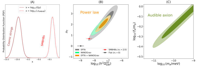
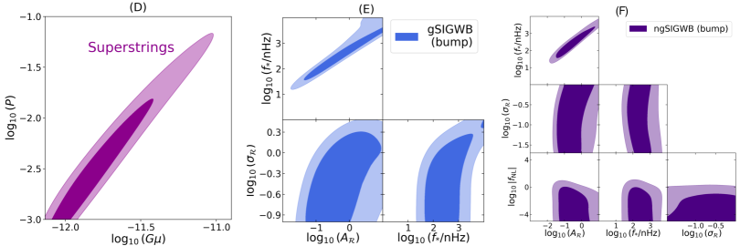
Figure 1: (A) 1D posteriors of field theory cosmic strings and SMBHBs with $n_{t}=2/3$, (B) 2D posterior for a PL signal (black and gray lines indicate the error band for $n_{t}=0$ and $2/3$, respectively) (C) 2D posterior for audible axions, (D) 2D posterior for superstrings, (E) and (F) 2D posteriors for Gaussian and non-Gaussian bump SIGWB, respectively.

Analysis.– For simplicity, we consider the data sets NG15 and EPTA-DR2new as independent, though we acknowledge the impact of overlapping pulsars on our findings. We postpone a proper combined analysis for when the full data become available. We extract physical information from free spectra chains, using Bayesian inference techniques, assuming each frequency point $f_{i}$ is independent, see supplementary material. In the following, we derive parameter constraints for scenarios $i)-vi)$.

Power Law (PL). The spectrum from canonical SMBHBs, inflation, and large scalar fluctuations with flat spectrum (cases of scenarios $(i)$, $(ii)$ and $(vi)$, respectively), can be parametrized by $\Omega_{\rm GW}^{(0)}=\mathcal{A}_{*}(f/f_{1y})^{n_{\rm t}}$, with free amplitude $\mathcal{A}_{*}$ at $f=f_{1y}$ and tilt $n_{t}=2/3$, free and $0$, respectively. Fitting simultaneously $\{\mathcal{A}_{*},n_{t}\}$ we obtain $\mathcal{A}_{*}=4.25_{-1.92}^{+3.05}\cdot 10^{-8}$ and $n_{t}=2.08_{-0.30}^{+0.32}$, at 68% CL. Fitting $\mathcal{A}_{*}$ while fixing $n_{t}=2/3$ or $n_{t}=0$, leads to $\mathcal{A}_{*}\big{|}_{2/3}=4.28_{-0.97}^{+0.99}\cdot 10^{-9}$ and $\mathcal{A}_{*}\big{|}_{0}=1.03^{+0.39}_{-0.26}\cdot 10^{-9}$, at 68% CL. Fig. 1-(A) shows the probability distribution function of $\mathcal{A}_{\rm SMBHB}$ (for $n_{t}=2/3$). Fig. 1-(B) shows the 1-$\sigma$ and 2-$\sigma$ contours of the full parameter space.

Broken Power Law (BPL). The GWB spectrum of scenario $(iii)$ on PhT’s can be captured by a BPL with $\Omega_{\rm GW}^{(0)}(f)\propto f^{n_{1}}$ and $\Omega_{\rm GW}^{(0)}(f)\propto f^{n_{2}}$ at low- ($f\ll f_{*}$) and high-frequencies ($f\gg f_{*}$), respectively. As the value of the tilts $\{n_{1},n_{2}\}$ are fixed for each PhT contribution, the peak’s frequency $f_{*}$ and amplitude $\mathcal{A}_{*}\equiv h^{2}\Omega_{\rm GW}^{(0)}(f_{*})$ are set uniquely by $\alpha$, $\beta$ and $T_{*}$. As the data constrains directly $\{f_{*},\mathcal{A}_{*}\}$, we have a clear handle on these fundamental parameters, see supplemental material. We obtain, at 68% CL, $T_{*}\in[6.2\cdot 10^{-3},9.0]$ GeV and $\beta/H_{*}\in[2.2,500]$ for bubble collisions (with $\alpha\gg 1$), $T_{*}\in[5.5,360]$ MeV and $\beta/H_{*}\in[1.0,15]$ for a signal from sound-waves + turbulence (with $\alpha\in[0.017,0.060]$), and $T_{*}\in[10^{-3},3.2]$ GeV for MHD turbulence.

Power Law with Cutoff (PLc). The spectrum of scenario (iv) on audible axions scales as $\propto f^{3/2}$ till it dies off exponentially at higher frequencies $f>f_{*}$. Fitting the cutoff frequency and peak amplitude $\{f_{*},\mathcal{A}_{*}\}$ from temaplte Eq. (6), leads to lower bounds on the axion mass and axion decay constant at 68% CL, as $m_{a}\gtrsim 8.0\cdot 10^{-11}$ meV and $f_{a}\gtrsim 1.3\cdot 10^{18}$ GeV, see Fig. 1-(C).

Cosmic Strings (CS). The broad spectrum in the CS scenario $(v)$, cf. Eq. (8), may exhibit a different frequency dependence than a power law at the PTA window. Fitting the data for field theory strings we find $\log_{10}(G\mu)=-9.90_{-0.19}^{+0.11}$, at 68% CL, see Fig. 1-(A). For superstrings instead, we find $\log_{10}(G\mu)=-11.83_{-0.15}^{+0.27}$ and $\log_{10}p=-2.63_{-0.31}^{+0.49}$, at 68% CL, see Fig. 1-(D).

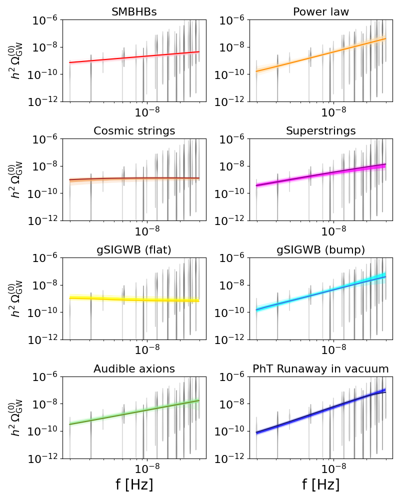
Figure 2: $h^{2}\Omega_{\rm GW}^{(0)}(f)$ for various cases. Solid-colored lines represent central values, while lighter (lightest) regions the 68% (95%) CL intervals. Dark and light gray violins are the EPTA and NANOGrav free spectrum data, respectively.

Scalar Induced GWB (SIGWB). For a Gaussian bump in scenario $(vi)$, we choose regions in the parameter space $\{\sigma_{\mathcal{R}}$, $f_{*}$, $A_{\mathcal{R}}\}$ that avoid primordial black hole (PBH) overproduction and are compatible with CMB, lensing, and LIGO/VIRGO observational bounds Green and Kavanagh (2021); Kavanagh (2019). We consider the non-linear relation between curvature and matter perturbations Young et al. (2019) and choose a real space top-hat window function to compute the variance and critical threshold of the smooth density. Fig. 1-(E) show the 1-$\sigma$ and 2-$\sigma$ contour plots, and Fig. 2 the reconstructed spectrum for the best-fit parameters, with 1-$\sigma$ and 2-$\sigma$ error bands. We notice that PTA data imposes $\sigma_{\mathcal{R}}\lesssim 3$ and provides a tighter bound than the previous data set Dandoy et al. (2023). The peak frequency is constrained to be $f_{*}\in[0.07,1.44]~{}{\mu\rm Hz}$, corresponding to a scale $k_{*}\in[4.57,88]\cdot 10^{7}$ Mpc^-1, at 68% CL. The amplitude $A_{\mathcal{R}}$ is quite large, though this depends on the value of $\sigma$. We obtain $A_{\mathcal{R}}\in[0.10,2.82]$ with $\sigma_{\mathcal{R}}\in[0.11,0.82]$ at 68% CL.

Concerning SIGWBs with pNG, we have considered a Gaussian component with bump spectrum, considering the non-linear relation between the smoothed density contrast and the linear curvature perturbation, extended to pNG Young (2022). The parameter space is $\{\sigma_{\mathcal{R}}$, $f_{*}$, $A_{\mathcal{R}},f_{\tt nl}\}$, subject to the perturbativity condition $A_{\mathcal{R}}f_{\tt nl}^{2}<1$ Adshead et al. (2021). The data impose $|f_{\tt nl}|\lesssim 2.34$ at 95% CL, see Fig. 1-(F).

Implications and model comparison.– We have fit PTA data to a variety of GWB spectra. If our fit to a PL spectrum is interpreted as an inflationary signal, this leads to connect the spectral tilt and amplitude at PTA scales to the tensor-to-scalar ratio $r$ at CMB scales, see supplemental material. Inputting our best-fit region $\{\mathcal{A}_{*},n_{t}\}$ into Eq. (S.7) leads to a tensor-to-scalar ratio (at the scale $k_{*}=0.05~{}{\rm Mpc^{-1}}$) within the range $r_{0.05}\in[4.37\cdot 10^{-14},3.47\cdot 10^{-9}]$ at 68% CL, well below current CMB constraints $r_{0.05}<0.032$ Tristram et al. (2022). Furthermore, a low-reheating temperature $T_{{\mathrm{reh}}}\lesssim 10.6$ GeV at 68% CL must be necessarily imposed to respect extra radiation $\Delta N_{\rm eff}$ constraints Allen and Romano (1999); Smith et al. (2006); Boyle and Buonanno (2008); Kuroyanagi et al. (2015); Caprini and Figueroa (2018); Ben-Dayan et al. (2019), cf. Eq. (S.10). While an inflationary signal which strongly violates the consistency relation $n_{t}=-r/8$, with a blue tilt as large as required by PTA data, $n_{t}\simeq 2$, is not impossible to conceive, adding on top the requisite of a low reheating temperature, makes extremely challenging to construct a viable model. An inflationary explanation of the PTA signal looks therefore somehow implausible.

Template	${\rm BF}_{\rm NANO}$	${\rm BF}_{\rm EPTA}$	${\rm BF}_{\rm comb}$	$\Delta{\rm AIC}_{\rm comb}$
PL($n_{t}=0$)	0.02	0.62	0.0014	10.24
PL($n_{t}=2/3$)	2.6	3.1	1.9	-5.20
PL($n_{t},\mathcal{A}_{*}$)	16	4.1	180	-12.25
field th. CS	0.18	1.3	0.019	5.22
super CS	29	3.3	58	-11.11
gSIGWB	120	15	1300	-13.54
ngSIGWB	66	8.7	780	-6.82
AA	36	2.7	130	-12.36
BPL	17	1.6	120	-0.19
PhTNR	8.5	8.1	150	-12.85
PhTRV	37	13	110	-12.34
MHD	26	3.9	210	-8.77

Table 1: Bayes factors $(\textrm{BF})$ for NANOGrav, EPTA and combined data sets, and Akaike Information Criterion $(\textrm{AIC})$ for the combined data sets. For the BF we have used the evidence of SMBHB model (2D Gaussian prior from Afzal et al. (2023)) to compare with, while the $\Delta$AIC is computed wrt SMBHB.

Two interesting cases emerge when fitting the data with a PL spectrum with fixed tilt $n_{t}$: a signal from SMBHBs with $n_{\rm t}=2/3$ Phinney (2001), and a SIGWB from large Gaussian scalar fluctuations with flat spectrum, which leads to a flat spectrum in $\Omega_{\rm GW}^{(0)}$ with $n_{t}=0$ De Luca et al. (2020, 2021). We obtain that $n_{t}=0$ and $n_{t}=2/3$ are ruled out by the combined data sets at $5.4\sigma$ and $3.9\sigma$, respectively, see Fig. 1-(B). Hence neither of these two scenarios is preferred by the PTA data.

We have also fit the data with a PL spectrum $\propto f^{3/2}$ up to a cutoff scale $f_{*}$, above which the spectrum is exponentially suppressed, cf. Eq. (6). This corresponds to an audible axion Machado et al. (2019, 2020); Co et al. (2021); Fonseca et al. (2020); Chatrchyan and Jaeckel (2021); Eröncel et al. (2022); Madge et al. (2022). PTA data implies lower bounds on the mass and decay constant of such axion, at 68% CL, as $m_{a}\gtrsim 8.0\cdot 10^{-11}$ meV and $f_{a}\gtrsim 1.3\cdot 10^{18}$ GeV, see Fig. 1-(B). As string theory does not prefer super-Planckian $f_{a}$ values Banks et al. (2003), imposing $f_{a}\leq m_{p}$ turns PTA data into a very tight constraint as $m_{a}=0.32_{-0.24}^{+1.48}$ peV. As pointed out by Geller et al. (2023), but contrary to previous NANOGrav 12.5-year data analysis Madge et al. (2023), the preferred parameter region is in tension with axion over-production and $\Delta N_{\rm eff}$ constraints.

Fitting the PTA signal also admits a BPL spectrum, which can be interpreted as a GWB originated in a first-order PhT. In this case, the low- and high-frequency PL tails $\{f^{n_{1}},f^{n_{2}}\}$ of the spectrum depend on the dominating contribution, with $\{f^{2.8}$, $f^{-1}\}$ for bubbles in a strong PhT, and $\{f^{3}$, $f^{-4}\}$ for sound waves plus a subdominant turbulence with $\{f^{2}$, $f^{-5/3}\}$ in a weak PhT. We obtain a central temperature as $T_{*}\simeq 20$ MeV ($\simeq 94$ MeV) for a strong (weak) PhT, suggesting a first-order PhT at the MeV scale which would be in tension with lattice QCD Aoki et al. (2006) and BBN prediction Bringmann et al. (2023). In the case of magneto-hydrodynamic (MHD) turbulence, the best-fit peak position can be translated Neronov et al. (2021a) into a primordial magnetic field of strength $B_{0}\simeq 23.3\mu$G and correlation length $l_{B}\simeq 0.25~{}{\rm pc}$, which is close to current constraints on primordial magnetic fields Ade et al. (2016); Jedamzik and Saveliev (2019); Neronov et al. (2021b); Acciari et al. (2023).

Fitting the PTA signal with field theory cosmic strings, leads to a very tight constraint of the associated energy scale as $\sqrt{\mu}\simeq 1.32^{+0.20}_{-0.24}\cdot 10^{14}~{}{\rm GeV}$. While this is $\mathcal{O}(10^{-2})$ smaller than standard Grand Unification scales $\sim 10^{16}~{}\rm GeV$, a wide variety of particle-physics models can still accommodate this value Vilenkin and Shellard (2000), see e.g. Kofman et al. (1996); Buchmuller et al. (2012); Buchmüller et al. (2013); Long and Wang (2019). Besides, the GWB spectrum should be also detectable by higher frequency future experiments, enabling us to learn about the cosmological history and particle physics above the BBN $\sim$MeV scale Cui et al. (2018, 2019); Gouttenoire et al. (2020a, b, 2021a, 2021b); Auclair et al. (2020b, 2023); Kitajima and Nakayama (2022); Ghoshal et al. (2023). Unfortunately, as we comment later, the GWB from field theory CS does not fit well PTA data. A cosmic superstring network, on the other hand, can fit very well the PTA data, thanks to accommodating a smaller energy scale $\sqrt{\mu}\simeq 1.56^{+0.48}_{-0.39}\cdot 10^{13}~{}{\rm GeV}$, while suppressing the intercommutation probability to $p=[1.13,7.06]\cdot 10^{-3}$.

Finally, we have fit PTA data with GWB spectra from large scalar fluctuations to second order. This leads to a stringent bound on primordial black hole (PBH) abundance. The data indicate that a GWB created by a Gaussian curvature perturbation with bump spectrum (gSIGWB-bump), requires a signal peak frequency $f_{*}\in[0.07,1.44]~{}{\mu\rm Hz}$ at 68% CL. This corresponds to a PBH distribution peaked around masses $M_{H}/M_{\odot}\in[1.5\cdot 10^{-5},5.6\cdot 10^{-3}]$, see supplemental material. Following Ref. Young et al. (2019), Fig. S.2 shows how the region of PTA best-fit is cut by the PBH over-abundance criterion $f_{\rm PBH}^{\rm tot}>1$, as well as by gravitational lensing. As the observational constraints are stronger than the over-abundance bound, our analysis implies that the PTA signal cannot correspond to an interpretation of PBH as the dark-matter totality. In any case, the best-fit PTA region can only survive for $\sigma_{\mathcal{R}}>1$. Next generation of PBH searches could resolve if the SIGWB could explain the origin of the PTA signal. We have also applied an analogous analysis for the case of a large curvature fluctuation with local pNG and Gaussian component with bump spectrum (ngSIGWB-bump), see Fig. 1-(F). Assuming perturbativity as $A_{\mathcal{R}}f_{\tt nl}^{2}<1$, PTA data provides a stringent constrain on the pNG parameter as $|f_{\tt nl}|\lesssim 2.34$ at 95% CL. This is a remarkable constraint on pNG at PTA scales, which we highlight are $\sim 8$ orders of magnitude smaller than CMB scales Akrami et al. (2020a). Our bound is conservative compared to bounds from PBH abundance, which depend strongly on the PBH formation and evolution details.

To determine which of the models is favored, we have performed a model selection/comparison Bayesian analysis. We employed two different criteria: the Bayes Factor (BF) $B_{i}=\rm{evidence}[\mathcal{H}_{i}]/\rm{evidence}[\mathcal{H}_{SMBHB}]$ (where $\mathcal{H}_{i}$ represents each model $i$ and SMBHB is a reference model with varying parameters extracted from two independent multivariate Gaussian prior distributions Afzal et al. (2023)), and the Akaike Information Criterion given by $\textrm{AIC}\equiv-2\ln\mathcal{L}+2k$ ($k$ is the number of parameters of the template). We report the values for all models analyzed in Table 1. We obtain that both for NANOGrav and EPTA, gSIGWB-bump shows the largest BFs, ${\rm BF}_{\rm NANO}=120$ and ${\rm BF}_{\rm EPTA}=15$, followed up closely by ngSIGWB-bump, with ${\rm BF}_{\rm NANO}=66$ and ${\rm BF}_{\rm EPTA}=8.7$. Additionally, the BF and $\Delta$AIC of the combined data indicate a very good fit for both gSIGWB and ngSIGWB signals, although we recall that there is an impact due to overlapping pulsars on the Bayesian search. There is also a “substantial” evidence for the audible axion and cosmic superstring models, both with ${\rm BF}_{\rm NANO}\sim 30$ and ${\rm BF}_{\rm EPTA}\sim 3$. While the superstring signal fits the data well, as pointed out in Afzal et al. (2023); Antoniadis et al. (2023c), the audible axion cannot explain the combined data because of its own relic constraints. We also remark that, as already found in Afzal et al. (2023), a simple PL with $n_{t}=2/3$ exhibits small BFs of order $\sim 2-3$ (also for the combined data set), indicating a poor/low quality fit. The remaining models examined in this paper show lower BF and AIC values, suggesting a reduced ability to fit the new data.

From our analysis we can draw some conclusions: while many models analyzed are able to fit the data, some cosmological scenarios fit better the data than SMBHBs. Among these, the gSIGWB+bump provides the best fit, with a very strong evidence in NANOGrav data and strong in EPTA data, in comparison to SMBHBs. A decisive evidence show up when the data sets are combined, with BF${}_{\rm comb}\simeq 1300$, though this number should not be taken too literally, given the caveat exposed on overlapping pulsars. Similarly, SIGWB with pNG also fit quite well the data, with BF${}_{\rm comb}\simeq 780$, and most importantly, leading to a stringent bound at the PTA scales as $|f_{\tt nl}|\lesssim 2.34$ at 95% CL. Concerning other cosmological models, we observe that, in agreement with Refs. Afzal et al. (2023); Antoniadis et al. (2023c), field theory strings do not fit well the data, whereas superstrings exhibit a good fit (though not as good as a SIGWB signals). However, as the superstring signal scaling $\propto 1/p$ is not well established, we advise to take with care this case. If eccentricity, environmental, or population effects are considered, Refs. Agazie et al. (2023c); Antoniadis et al. (2023c); Ellis et al. (2023a) show that SMBHBs can still fit well the data. Therefore, no clear conclusion about the origin of the signal can be reached at this point. While the detection of a GWB by PTA collaborations Agazie et al. (2023a); Antoniadis et al. (2023a); Reardon et al. (2023); Xu et al. (2023) has opened an exciting window for astrophysics, early universe cosmology and BSM physics, further data and analysis are still needed to reach robust conclusions.

Note added: Taken individually, some of our results overlap with the new physics searches by NANOGrav and EPTA collaborations Afzal et al. (2023); Antoniadis et al. (2023c), as well as with recent studies Franciolini et al. (2023a); Ellis et al. (2023b); Franciolini et al. (2023b); Vagnozzi (2023); Cai et al. (2023b). There are however some differences. For example, ours is a NANOGrav and EPTA combined data Bayesian analysis, which improves some of the model constraints. Furthermore, we have considered a smoothing procedure of the GWB spectra per bin. Model-wise, we have extended the search to audible axions and SIGWBs with pNG. The day before we submitted our work, two studies appeared in the ArXiv considering PTA constraints on local pNG Liu et al. (2023); Wang et al. (2023), both presenting similar constraints on $f_{\tt nl}$.

Acknowledgements – We thank Stas Babak, Matthias Koschnitzke, Andrea Mitridate, Gabriele Perna, Hippolyte Quelquejay Leclere, Kai Schmitz, Géraldine Servant, and Zach Weiner for useful discussions. DGF (ORCID 0000-0002-4005-8915) is supported by a Ramón y Cajal contract with Ref. RYC-2017-23493. This work was supported by Generalitat Valenciana grant PROMETEO/2021/083, and by Spanish Ministerio de Ciencia e Innovacion grant PID2020-113644GB-I00. AR acknowledges financial support from the Supporting TAlent in ReSearch@University of Padova (STARS@UNIPD) for the project “Constraining Cosmology and Astrophysics with Gravitational Waves, Cosmic Microwave Background and Large-Scale Structure cross-correlations”.

Supplemental Material

This supplemental material contains more details on the data analysis used in the main text. The translation from the GWB templates’ parameters into the particle physics and cosmological parameters is also provided. As examples, we link the power-law and broken power-law templates to the GWB from primordial inflation and first-order PhT, respectively. Lastly, we discuss briefly the primordial black hole and the scalar-perturbation power-spectrum constraints relating to the scalar-induced GWB interpretation.

Assumptions.– In all our computations, we have assumed standard $\Lambda$CDM cosmology for the cosmic history, with $\Omega_{\rm rad}^{(0)}\simeq 9.2\cdot 10^{-5}$, $h\simeq 0.68$, and the evolution of the relativistic degrees of freedom $g_{*}(T)$ and $g_{*,s}(T)$ obtained from App.C of Saikawa and Shirai (2018). The (reduced) Planck mass is $m_{p}\equiv(8\pi G)^{-1/2}\simeq 2.44\cdot 10^{18}$ GeV.

Input Data.– The effect of GWB is characterized, in the PTA time-of-arrival data, as the time-correlated stochastic process, parametrized by the one-sided power spectral density $S(f_{i}=i/T_{\rm obs})$ for each frequency bin that is a harmonic $i^{\rm th}$ of the inverse of observational time $T_{\rm obs}^{-1}$ Afzal et al. (2023). This turns into the power spectrum of the fraction energy density in GW today as Allen and Romano (1999),

$$\Omega_{\rm GW}^{(0)}(f)=\frac{8\pi^{4}f_{\rm yr}^{5}}{H_{0}^{2}}S(f)\left(\frac{f}{f_{\rm yr}}\right)^{5},$$ (S.1)

In the case in which the signal PSD can be parametrized with a power law like, we have

$$S(f)=\frac{A_{\rm CP}^{2}}{12\pi^{2}}\left(\frac{f}{f_{\rm yr}}\right)^{-\gamma}{f_{\rm yr}}^{-3}~{}~{}~{}~{}~{}\Leftrightarrow~{}~{}~{}~{}\Omega_{\rm GW}^{(0)}(f)=\frac{2\pi^{2}f_{\rm yr}^{2}}{3H_{0}^{2}}A_{\rm CP}^{2}\left(f\over f_{\rm yr}\right)^{5-\gamma}\,.$$ (S.2)

The “violins” in the plots represent the free spectrum marginalized probability distribution function (PDF) of the amplitude of the sine-cosine Fourier pair (i.e., $\sqrt{S(f)/T}$ in seconds) for all frequencies $f_{i}$’s.

I More details on data analysis

This section provides a more detailed explanation of the data analysis technique employed in this work. For what concerns the likelihood definition, we proceed as follows. We start by performing a Gaussian kernel smoothing of the histograms built from the free spectrum chains.The result of this procedure is used to estimate probability distribution functions (PDFs) for signal amplitude in the frequency bins $f_{k}$, which are thus assumed to be independent from one another. In particular, under these assumptions, the full log-likelihood is represented as

$$\ln\mathcal{L}=\sum_{k}\ln p_{k}(\mathcal{D}_{k}|\vec{\theta},)\;,$$ (S.3)

where $\vec{\theta}$ is the parameter vector of the models, and $\mathcal{D}_{k}$ and $p_{k}$ are the data chains and likelihoods respectively. Some signals, such as the scalar-induced GWB, exhibit variations on frequency scales that are (much) smaller than the experiment resolution $\Delta f=1/T_{\rm tot}$ (with $T_{\rm tot}$ as the total observation time). Since detection is based on integrated power within frequency bins of width $\Delta f$, the data cannot capture these variations. To account for this, we smooth the templates by averaging over bins of size $\Delta f$. The log-posterior is defined as the sum of the log-likelihood in eq. S.3 and of the (log)-priors, defined in the following section. Finally, the parameter space is sampled using the Nested Sampler Polychord Handley et al. (2015a, b) via the Cobaya Torrado and Lewis (2021) interface, as well as the MCMC sampler Lewis (2013).

Prior.– For each model, we assign uniform/log-uniform priors to all the parameters, ensuring wide ranges to avoid impact on parameter estimation. A collection of the ranges used in the analysis is reported in table S.II.

White-noise.– In analogy with the approach of Afzal et al. (2023); Antoniadis et al. (2023a), in the full frequency analysis, we assume that a flat (white noise-like) component might be present in the data. In the referenced works, this additional component was included on top of a low-frequency power law behavior, giving rise to a broken power law model with a flat tilt at large frequencies. In the present work, we add this secondary component to all the models we discuss. This procedure automatically selects the relevant bins to constrain the cosmological signal from the full frequency range and models the high-frequency part of the spectrum in terms of the extra flat component. We have compared the compatibility of the results obtained with the full frequency analysis (including the additional flat component) with the results obtained using only the low frequency part of the spectrum and found good agreement for most models.

II From Templates to Particle-Physics and Cosmological Parameters

This section provides the dictionary between the templates’ parameters and the information about particle physics and cosmology. In the main texts, some of the templates are already parametrized as the particle physics parameters, i.e., cosmic strings $G\mu$, the audible axion $\{m_{a},f_{a}\}$, and the scalar-induced GW with the parameters of the curvature-perturbation power spectrum. So we focus on the power-law template, which explains GWB from primordial inflation, and the broken power law, which is compatible with first-order phase transitions in many scenarios. The central value and the error intervals of the physical parameters, quoted in the main text, are obtained by doing analysis directly on such parameters.

Power-law.– Apart from the astrophysical GWB from SMBHBs whose spectral tilt is fixed to $2/3$, the GWB from primordial inflation beyond the vanilla slow-roll inflation can lead to a GWB with an arbitrary tilt.

Primordial Inflation. The spectrum of GW energy density fraction today (assuming the $\Lambda$CDM cosmology) reads Caprini and Figueroa (2018),

$$h^{2}\Omega_{\rm GW}^{(0)}(k)=\frac{3}{128}\Omega_{\rm rad}^{(0)}h^{2}\mathcal{P}_{t}(k)\left[\frac{1}{2}\left(\frac{k_{\rm eq}}{k}\right)^{2}+\frac{16}{9}\right]\xrightarrow{k\gg k_{\rm eq}}\frac{\Omega_{\rm rad}^{(0)}h^{2}}{24}\mathcal{P}_{t}(k),$$ (S.4)

with $\mathcal{P}_{t}(k)$ the primordial tensor power spectrum, and $k_{\rm eq}\simeq 1.3\cdot 10^{-2}~{}{\rm Mpc^{-1}}$ the comoving scale at matter-radiation equality. The second step is justified because the comoving scale around the PTA scale is much larger than $k_{\rm eq}$, i.e., the GW wavenumber-frequency conversion is $k=2\pi f$ or,

$$k=6.25\cdot 10^{5}~{}{\rm Mpc}^{-1}\left(\frac{f}{\rm nHz}\right).$$ (S.5)

With a power-law primordial tensor perturbation, the GW spectrum is also a power-law. We parametrize it in terms of the CMB measurement at the pivot scale $k_{\rm pivot}=0.05~{}{\rm Mpc^{-1}}$,

$$\mathcal{P}_{t}(k)=rA_{s}\left(\frac{k}{k_{\rm pivot}}\right)^{n_{t}},$$ (S.6)

where $r$ is the tensor-to-scalar ratio whose upper bound is $r\leq 0.032$ (Planck, BICEP/Keck, BAO) Tristram et al. (2022), $A_{s}$ is the primordial scalar perturbation measured at $k_{\rm pivot}$ whose value is constrained to $A_{s}\simeq 2.1\cdot 10^{-9}$ (TT, TE, EE+low-E+lensing) Akrami et al. (2020b), and $n_{t}$ is the spectral tilt as in Eq. (2). We can rewrite Eq. (S.4) in terms of frequency as, using Eqs. (S.5) and (S.6),

$$h^{2}\Omega_{\rm GW}^{(0)}(f)\simeq 1.19\cdot 10^{-16}\left(\frac{r}{0.032}\right)\left(\frac{A_{s}}{2.1\cdot 10^{-9}}\right)\left(\frac{f}{f_{\rm pivot}}\right)^{n_{t}},$$ (S.7)

where $f_{\rm pivot}\simeq 8\cdot 10^{-17}$ Hz is the frequency corresponding to the pivot scale $k_{\rm pivot}$. For given amplitude $\Omega_{\rm GW}^{(0)}(f_{*})$ and frequency $f_{*}$, an increasing $n_{t}$ gives a smaller $r$. From the analysis in the main text, the best-fitted spectrum is highly red-tilted and corresponds to the tensor-to-scalar ratio of $r\simeq 10^{12}$, which is firmly excluded by the CMB bound. Nonetheless, the 2$\sigma$ region prefers the blue-tilted spectrum and has the tensor-to-scalar ratio of $r\in[5\times 10^{-4},0.032]$; see Fig. S.1. The highly blue-tilted (large $n_{t}$) GWB could be in tension with the extra-radiation bound. The total GW energy density fraction should not exceed that of the extra radiation Allen and Romano (1999); Smith et al. (2006); Boyle and Buonanno (2008); Kuroyanagi et al. (2015); Caprini and Figueroa (2018); Ben-Dayan et al. (2019) parametrized by the number of extra neutrino species $\Delta N_{\nu}$,

$$\int_{f_{\rm BBN}}^{f_{\rm reh}}\frac{df}{f}\Omega_{\rm GW}^{(0)}\leq 5.6\cdot 10^{-6}\Delta N_{\nu}~{}\xrightarrow{\rm Eq.~{}\eqref{eq:GWB_inflation_in_f}}f_{\rm reh}\lesssim f_{\rm BBN}\left[1+(4.3\cdot 10^{9})\,n_{t}\left(\frac{f_{\rm pivot}}{f_{\rm BBN}}\right)^{n_{t}}\left(\frac{\Delta N_{\nu}}{0.2}\right)\left(\frac{0.032}{r}\right)\left(\frac{2.1\cdot 10^{-9}}{A_{s}}\right)\right]^{\frac{1}{n_{t}}},$$ (S.8)

where we integrated from the reheating scale $f_{\rm reh}$ to BBN (or CMB) scale $f_{\rm BBN}$ in the second step. Using that the perturbation re-enters the horizon at $k=a(T)H(T)$ when the Universe has temperature $T$, we obtain the conversion,

$$f=1.84~{}{\rm nHz}\left(\frac{T}{100~{}\rm MeV}\right)\left(\frac{g_{*}(T)}{10.75}\right)^{\frac{1}{2}}\left(\frac{g_{*,s}(T)}{10.75}\right)^{-\frac{1}{3}}.$$ (S.9)

The BBN scale $T_{\rm BBN}\simeq\rm MeV$ corresponds to $f_{\rm BBN}\simeq 1.84\cdot 10^{-11}$ Hz. From Eq.(S.8), the extra-radiation bound becomes a constraint on the reheating temperature of the Universe,

$$T_{\rm reh}\lesssim~{} {0.68~{}\rm MeV}\left(\frac{f_{\rm BBN}}{1.84\cdot 10^{-11}~{}\rm Hz}\right)\left(\frac{106.75}{g_{*}(T_{\rm reh})}\right)^{\frac{1}{2}}\left(\frac{106.75}{g_{*,s}(T_{\rm reh})}\right)^{-\frac{1}{3}}\times$$

$$\times\left[1+(4.3\cdot 10^{9})\,n_{t}\left(\frac{f_{\rm pivot}}{f_{\rm BBN}}\right)^{n_{t}}\left(\frac{\Delta N_{\nu}}{0.2}\right)\left(\frac{0.032}{r}\right)\left(\frac{2.1\cdot 10^{-9}}{A_{s}}\right)\right]^{\frac{1}{n_{t}}}.$$ (S.10)

For a power-law GW spectrum in PTA range – $h^{2}\Omega_{\rm GW}^{(0)}(f_{*})\simeq 10^{-10}$ and $f_{*}\simeq\rm nHz$ – with $A_{s}\simeq 2.1\cdot 10^{-9}$ and $r=0.032$, the spectral tilt is $n_{t}\simeq 0.73$ and the bound on the reheating temperature reads $T_{\rm reh}\lesssim 44~{}\rm TeV$. From Fig. S.1, the tip of the 2$\sigma$ region that survives the CMB constraint on $r$ requires a low-scale reheating temperature $T_{\rm reh}<0.1-1$ TeV.

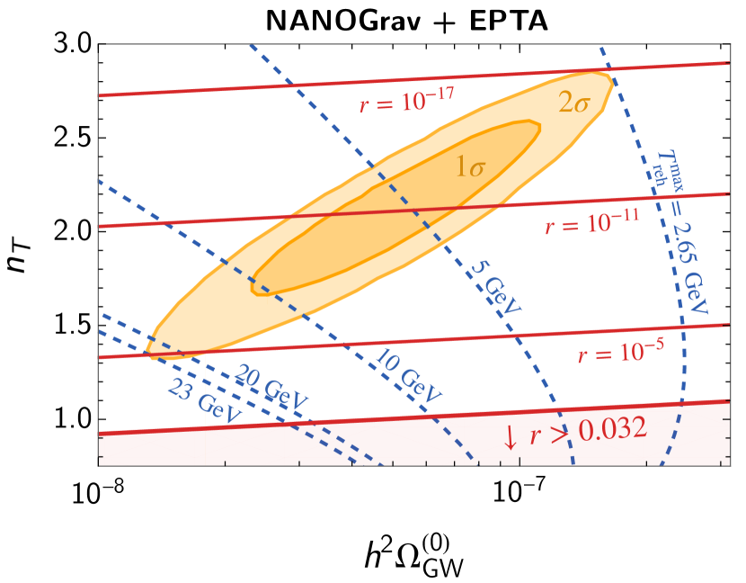
Figure S.1: The CMB observations tightly constrain the PTA-signal interpretation as the inflationary GWB (blue contours). The bound on the tensor-to-scalar ratio (in red) excludes the region with $r>0.032$. The BBN-$N_{\rm eff}$ bound requires a low-scale reheating: $T_{\rm reh}<10.6$ GeV, at 68% CL.

Lastly, the required $T_{\rm reh}$ in Eq. (S.10) does not guarantee that the extra-radiation bound is not further violated at $f>f_{\rm reh}$. Because the completion of reheating and the end of inflation can be separated by the reheating phase, which is not necessarily radiation-dominated. Assuming the dominant energy density is a fluid of equation-of-state $\omega$, the GWB from inflation is affected through its transfer function and receives a tilt Giovannini (1998, 1999); Boyle and Buonanno (2008),

$$\Omega_{\rm GW}^{(0)}(f)\propto\mathcal{P}_{t}(f)f^{-2(1-3\omega)/(1+3\omega)}\xrightarrow{\rm Eq.~{}\eqref{eq:tensor_power_spec_param}}\Omega_{\rm GW}^{(0)}(f)\propto f^{n_{t}-2(1-3\omega)/(1+3\omega)}.$$ (S.11)

If the extra-radiation bound is saturated at $T_{\rm reh}$, the reheating phase is required to have $\omega\lesssim(2-n_{t})/(6+3n_{t})$.

Broken power law.– GWBs from short-lasting sources, e.g., first-order PhT, and the particle production of the audible axion, usually have a peaked shape. Since the UV tail of the audible axion’s spectrum is not a power law but an exponential cut-off in Eq. (6), the broken power-law template represents only the case of PhT. The peak position is composed of the peak amplitude today, $\Omega_{\rm GW}^{(0)}=\Omega_{\rm rad}^{(0)}\mathcal{G}(T_{*})\sum_{i}{\Omega}_{{\rm GW},i}$ with $\mathcal{G}\equiv[g_{*}(T_{*})/g_{*}(T_{0})][g_{*,s}(T_{*})/g_{*,s}(T_{0})]^{-4/3}$ and ${\Omega}_{{\rm GW},i}$ in Eq. (3), and the peak frequency today $f_{*}$ defined in Tab. S.I. We can thus convert the fitted template’s parameters into the PhT parameters in the three scenarios: a) the bubble-dominated case for a strong PhT, b) the sound-wave-dominated case for a weak PhT, and c) the turbulence-dominated for a medium strength. Moreover, we also consider case c) the turbulence from magneto-hydrodynamic (MHD) eddies, whose GW spectrum relates to the primordial magnetic field and which might or might not rely on PhT.

	Bubbles Huber and Konstandin (2008)	Sound-wave Hindmarsh et al. (2015)	Turbulence Caprini et al. (2009)
$\mathcal{N}_{i}$	1	0.16	20
$\Delta_{i}(v_{\rm w})$	$\frac{0.11\,v_{\rm w}^{3}}{0.42+v_{\rm w}^{2}}$	$v_{\rm w}$	$v_{\rm w}$
$p_{i}$	2	2	3/2
$q_{i}$	2	1	1
$s_{i}(f,f_{*})$	$\frac{3.8(f/f_{*})^{2.8}}{1+2.8(f/f_{*})^{3.8}}$	$\left(\frac{f}{f_{*}}\right)^{3}\left[\frac{7}{4+3(f/f_{*})^{2}}\right]^{\frac{7}{2}}$	$\frac{(f/f_{*})^{3}}{(1+f/f_{*})^{11/3}\left(1+8\pi f/\tilde{H}_{*}\right)}$
$f_{*}$	$11{\rm nHz}\left(\frac{0.62}{1.8-0.1v_{\rm w}+v_{\rm w}^{2}}\right)\mathcal{F}$	$13{\rm nHz}~{}v_{\rm w}^{-1}\mathcal{F}$	$19{\rm nHz}~{}v_{\rm w}^{-1}\mathcal{F}$

Table S.I: Parameters and functions for three types of the GWB from first-order PhTs, taken or derived from Ref. Breitbach et al. (2019).

$${\rm with}~{}~{}\mathcal{F} \equiv\left(\frac{\beta}{H_{*}}\right)\left(\frac{T_{*}}{0.1~{}{\rm GeV}}\right)\left(\frac{g_{*}(T_{*})}{10.75}\right)^{\frac{1}{2}}\left(\frac{g_{*,s}(T_{*})}{10.75}\right)^{-\frac{1}{3}},$$ (S.12)

$${\rm and}~{}~{}\tilde{H}_{*} \equiv H_{*}\left(\frac{a_{*}}{a_{0}}\right)\simeq 11~{}{\rm nHz}\left(\frac{T_{*}}{0.1~{}{\rm GeV}}\right)\left(\frac{g_{*}(T_{*})}{10.75}\right)^{\frac{1}{2}}\left(\frac{g_{*,s}(T_{*})}{10.75}\right)^{-\frac{1}{3}}.$$ (S.13)

a) Bubbles. According to the envelope approximation Huber and Konstandin (2008), the shape of the GWB has the IR tail with $\Omega_{\rm GW}\propto f^{2.8}$ and the UV tail with $\Omega_{\rm GW}\propto f^{-1}$. If there is a vacuum-dominated epoch or the so-called super-cooling phase ($\alpha\gg 1$), a strong first-order PhT happens in a vacuum, and the collisions among bubble walls source the dominant GW signal. With Eq. (3) and Tab. S.I, we translate the peak position – the peak frequency today $f_{*}$ and the amplitude $\Omega_{\rm GW}^{(0)}(f_{*})$ – of the GWB into the PhT parameters:

$$\left(\frac{\beta}{H_{*}}\right)_{\rm b} \simeq 206\left[\Delta_{\rm b}(v_{\rm w})\kappa_{\rm b}^{2}\mathcal{G}(T_{*})\left(\frac{10^{-9}}{h^{2}\Omega_{\rm GW}^{(0)}(f_{*})}\right)\right]^{1/2},$$ (S.14)

$$\left(T_{*}\right)_{\rm b} \simeq 0.48~{}{\rm MeV}\left(\frac{f_{*}}{10~{}\rm nHZ}\right)\left(\frac{h^{2}\Omega_{\rm GW}^{(0)}(f_{*})}{10^{-9}}\right)^{1\over 2}\left(\frac{g_{*,s}(T_{*})}{g_{*}(T_{*})}\right)\left(\frac{1.8-0.1v_{\rm w}+v_{\rm w}^{2}}{0.62}\right)\Delta_{\rm b}^{-\frac{1}{2}}\kappa_{\rm b}^{-1}.$$ (S.15)

Typically, the vacuum energy is efficiently converted into the energy of the bubbles $\kappa_{\rm b}=1$, and the wall velocity reaches the speed of light $v_{\rm w}\to 1$ (and $\Delta_{\rm b}\approx 0.08$). For the range compatible with PTA observation, this strong PhT following the vacuum-dominated phase completes at $T_{*}\sim$MeV and can obstruct BBN Bringmann et al. (2023).

b) Sound wave. According to Ref. Hindmarsh et al. (2015), the shape of the GWB has the IR tail with $\Omega_{\rm GW}\propto f^{3}$ and the UV tail with $\Omega_{\rm GW}\propto f^{-4}$. The sound-wave contribution dominates when the PhT is not too strong, and the bubbles expand in the background thermal plasma and reach the terminal velocity (so-called non-runaway scenario). The peak position in Eq. (3) and Tab. S.I can be translated into PhT parameters ($\alpha$, $\beta/H_{*}$, $T_{*}$) by,

$$\left(\frac{\beta}{H_{*}}\right)_{\rm sw} \simeq 68\left(\frac{10^{-9}}{h^{2}\Omega_{\rm GW}^{(0)}(f_{*})}\right)\mathcal{G}(T_{*})v_{\rm w}\left[\frac{(1+\alpha)^{2}\alpha^{-2}\kappa^{-2}_{\rm sw}(\alpha)}{100}\right]^{-1},$$ (S.16)

$$\left(T_{*}\right)_{\rm sw} \simeq 1.5~{}{\rm MeV}\left(\frac{f_{*}}{10~{}\rm nHZ}\right)\left(\frac{h^{2}\Omega_{\rm GW}^{(0)}(f_{*})}{10^{-9}}\right)\left[\frac{10.75}{g_{*}(T_{*})}\right]^{\frac{3}{2}}\left[\frac{g_{*,s}(T_{*})}{10.75}\right]^{\frac{5}{3}}\left[\frac{(1+\alpha)\alpha^{-1}\kappa^{-1}_{\rm sw}(\alpha)}{10}\right]^{2}.$$ (S.17)

where the efficiency factor is $\kappa_{\rm sw}(\alpha)\simeq\alpha(0.73+0.083\sqrt{\alpha}+\alpha)^{-1}$ Espinosa et al. (2010). The numerator of the last bracket in the $T_{*}$ expression is $\simeq 84$ and 6.2 for $\alpha=0.1$ and 0.5, respectively. Note that there is degeneracy among $\alpha$, $\beta/H_{*}$, and $T_{*}$, which could be further broken by considering a UV completion of this low-$T$ first-order PhT.

c) Turbulence. From Ref. Caprini et al. (2009), the shape of the GWB is a double-broken power-law spectrum. The slope far from the peak in the IR is $\Omega_{\rm GW}\propto f^{3}$ from causality. The intermediate IR scale $\tilde{H}_{*}<f<f_{*}$ with $\Omega_{\rm GW}\propto f^{2}$ corresponding to the time scale of the turbulence, and the UV tail with $\Omega_{\rm GW}\propto f^{-5/3}$. Typically during PhT, the GW from turbulence is accompanied by the more dominant sound-wave contribution (i.e., $\kappa_{\rm turb}<\kappa_{\rm sw}$). In our analysis, we consider both sound-wave and turbulence in the case of weak PhT.

MHD turbulence.–Usually, the turbulence arises as MHD eddies due to the bubble motion during first-order PhT or some other mechanisms (e.g., Kamada and Shin (2020)) unrelated to PhT. The GWB is sourced by the magnetic anisotropy and has the energy density fraction at the production: $\Omega_{\rm GW}^{*}\sim 3(\Omega_{B}^{*})^{2}(H_{*}\mathcal{T})^{2}$ Neronov et al. (2021a) where $\Omega_{B}^{*}=B_{*}^{2}/(2\rho_{c,*})$ is the magnetic energy-density fraction, $*$ denotes the time of GW emission, and the sourcing-time scale related to size and velocity of turbulence $\mathcal{T}\sim l_{*}/v_{A}\lesssim H_{*}^{-1}$ with $v_{A}\simeq\sqrt{2\Omega_{B}^{*}}$ the Alfvén speed. The GW energy density becomes $\Omega_{\rm GW}^{*}\sim\frac{3}{2}\Omega_{B}^{*}(H_{*}l_{*})^{2}$. Nonetheless, depending on the detail of turbulence, the scaling can vary $\Omega_{\rm GW}^{*}\sim(\Omega_{B}^{*})^{n}(H_{*}l_{*})^{2}$ with $n\in[1,2]$. The GW spectrum today peaks at amplitude $\Omega_{\rm GW}^{(0)}=\Omega_{\rm rad}^{(0)}\mathcal{G}(T_{*})(\Omega_{B}^{*})^{n}(H_{*}l_{*})^{2}$ and frequency today $f_{*}=\frac{2}{l_{*}}\cdot\frac{a_{*}}{a_{0}}$ Neronov et al. (2021a). For simplicity, we consider the case of the largest processed eddies (LPE) i.e., maximized $l_{*}=v_{A}/H_{*}$ and the GW spectrum. The peak position – the amplitude and frequency – is related to the magnetic energy fraction and the temperature of the GW production,

$$\Omega_{B}^{*} \simeq\left[1.4\cdot 10^{-5}\left(\frac{h^{2}\Omega_{\rm GW}^{(0)}(f_{*})}{10^{-9}}\right)\left(\frac{10.75}{g_{*}(T_{*})}\right)\left(\frac{g_{*,s}(T_{*})}{10.75}\right)^{\frac{4}{3}}\right]^{1/(n+1)},$$ (S.18)

$$f_{*} \simeq 16.1~{}{\rm nHz}\left(\frac{T_{*}}{\rm MeV}\right)\left(\frac{10^{-2}}{\Omega_{B}^{*}}\right)^{1\over 2},$$ (S.19)

We can also characterize the MHD turbulence by the magnetic field strength $B_{0}$ and the magnetic-field correlation length scale $l_{B}\equiv l_{*}(a_{0}/a_{*})$ as observed today,

$$B_{0}=0.4~{}{\rm\mu G}\left(\frac{\Omega_{B}^{*}}{10^{-2}}\right)^{\frac{1}{2}}\left(\frac{g_{*}(T_{*})}{10.75}\right)^{\frac{1}{2}}\left(\frac{10.75}{g_{*,s}(T_{*})}\right)^{\frac{2}{3}},~{}~{}l_{B}\simeq 1.95~{}{\rm pc}\left(\frac{10~{}{\rm nHz}}{f_{*}}\right).$$ (S.20)

Cosmic Strings.– We assume that a string network loses energy only through GW emission of loops. We sum up to $j=10^{5}$ modes of loop oscillations. More complicated CS scenarios, e.g. small-loop population Lorenz et al. (2010) or meta-stable strings Buchmuller et al. (2020a, 2021, b), can alter the fittings to PTA data, see Ref. Leclere et al. (2023); Afzal et al. (2023). We also note that we consider field theory CS from a gauge symmetry, discarding the global symmetry case, whose Goldstone-boson emission leads to a strong $\Delta N_{\rm eff}$ bound Chang and Cui (2022); Gorghetto et al. (2021). See Servant and Simakachorn (2023) for the best-fitted result and constraints on global-(axionic)-string SGWB obtained from the recent analysis of the NG15 data set.

III Constraints on scalar-induced gravitational waves

Large scalar perturbations at small scales, unbounded by CMB, are constrained by their direct consequences and many observations. We classify two types of constraints:

Primordial black holes.– Sourced by the scalar perturbation, the energy density perturbations collapse into the primordial black holes (PBH) Hawking (1971); Carr and Hawking (1974); Carr (1975) whose abundance is subjected to the PBH over-abundance and many observational bounds (e.g., gravitational lensing and LVK merger events) Green and Kavanagh (2021); Kavanagh (2019). Starting from the scalar perturbation in Eq. (13), we use the peak theory method in Ref. Young et al. (2019) with a real-space top-hat window function (with $\gamma=0.36$, $\kappa=4$, and $\delta_{c}=0.55$) to calculate the total PBH abundance today, parametrized by $f_{\rm PBH}^{\rm tot}$ the total fraction of the cold dark matter today. We also include the non-linear effect between the primordial scalar and the energy density perturbations.

Since the collapse happens when the scalar perturbation re-enters the horizon, many populations of PBH can be formed from a broad scalar power spectrum along the cosmic history. However, the spectral shape of the PBH abundance over mass range inherits that of the primordial scalar perturbation. For the SIGW peaked at frequency $f_{*}$, the scale of the scalar-perturbation peak re-enters the horizon and collapses into the peak of PBH mass distribution with mass defined by the horizon mass $M_{H}$, i.e., the total energy density enclosed within the Hubble volume at temperature $T$,

$$M_{H}=\frac{4\pi}{3}H^{-3}\left(3M_{{}_{\mathrm{Pl}}}^{2}H^{2}\right)\simeq 44\,M_{\odot}\,\left(\frac{g_{*}(T)}{10.75}\right)^{\frac{1}{2}}\left(\frac{10.75}{g_{*s}(T)}\right)^{\frac{2}{3}}\left(\frac{10^{-9}\,{\rm Hz}}{f_{*}}\right)^{2},$$ (S.21)

where $M_{\odot}\simeq 1.988\times 10^{30}$ kg is the Solar mass, and we used the frequency-temperature relation (S.9). For a typical frequency of SIGW in PTA ($f_{*}\simeq 1-10$ nHz), the PBH is populated in the mass range of $M_{H}\simeq\mathcal{O}(0.4-40)M_{\odot}$.

The most conservative constraint is the PBH over-abundance $f_{\rm PBH}^{\rm tot}>1$, while many observations also exclude the PBH abundance for $f_{\rm PBH}^{\rm tot}<1$ over a wide range of masses Green and Kavanagh (2021); Kavanagh (2019). There are two dominant constraints for the Solar-mass PBH compatible with PTA interpretation: the LVK mergers, individual events and stochastic background, and the gravitational lensing constraints. We translate the bounds on the monochromatic PBH mass in Ref. Green and Kavanagh (2021) using the method outlined in Ref. Carr et al. (2017) for our extended PBH mass distribution. Fig. S.2 shows the constraints (PBH over-abundance, lensing, and LVK mergers) on the log-normal scalar perturbation. We also calculate the PBH abundance in the presence of the pNG scalar perturbation by applying the simplifying technique of Ref. Young (2022) to the procedure of the Gaussian case.

CMB and $\mu$-distortion.– Though the scalar perturbation power spectrum peaks at the scale of PTA, its tail at scales larger than PTA ($k\lesssim 10^{6}~{}{\rm Mpc}^{-1}$) can be constrained for a too broad spectrum. First, the sizeable scalar perturbation sources the density fluctuation, dissipating into photon fluid and causing the $\mu$-distortion of the CMB spectrum Chluba et al. (2012); Kohri et al. (2014). Another constraint arises when the spectrum is broad and large to contradict the CMB observations Hunt and Sarkar (2015). By translating the bounds in Ref. Inomata and Nakama (2019), we find no such bound entering the shown parameter spaces of Fig. S.2.

2nd Order Scalar Induced GWB (Gaussian)

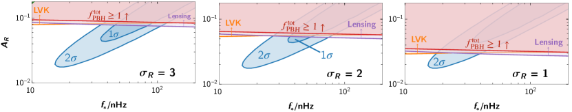
Figure S.2: Constraints on the Gaussian scalar-perturbation bumps in Eq. (13) from PBH abundance (over-abundance, lensing, LVK mergers) and other constraints ($\mu$-distortion). The parameters are $\{\sigma$, $f_{*}$, $A_{\mathcal{R}}\}$. The 2OSI GW interpretation of the PTA signal (in blue) survives but cannot account for the dark matter totality.

Parameter	Description	Prior
	Power law (PL)
$\mathcal{A}^{(*)}_{\rm inf}$	Amplitude of the signal at $f_{*}=f_{1\rm yr}$	log-uniform [$10^{-20},10^{-4}$]
$n_{t}$	Spectral tilt	uniform [$-4,6$]
	SMBHBs (PL $n_{t}=2/3$)
$\mathcal{A}^{(*)}_{\rm 2/3}$	Amplitude of the signal at $f_{*}=f_{1\rm yr}$	log-uniform [$10^{-14},10^{-6}$]
	Flat (PL $n_{t}=0$)
$\mathcal{A}^{(*)}_{\rm 0}$	Amplitude of the signal at $f_{*}=f_{1\rm yr}$	log-uniform [$10^{-13},10^{-4}$]
	Field-theory Cosmic strings (field th. CS)
$G\mu$	Cosmic-string tension	log-uniform [$10^{-14},10^{-6}$]
	Cosmic super-strings (super CS)
$G\mu$	Cosmic-string tension	log-uniform [$10^{-14},10^{-6}$]
$p$	Inter-commutation probability	log-uniform [$10^{-3},1$]
	Broken power law (BPL)
$\mathcal{A}_{*}$	Peak amplitude	log-uniform [$10^{-14},10^{-7}$]
$f_{*}$ [nHz]	Peak frequency	log-uniform [$10^{-2.5},10^{4.5}$]
$n_{1}$	Low-frequency tilt $f\ll f_{*}$	uniform [$-8,8$]
$n_{2}$	High-frequency tilt $f\gg f_{*}$	uniform [$-8,8$]
	Audible axion (AA)
$f_{a}$ [$m_{p}$]	Axion decay constant	log-uniform [$10^{-4},10^{2}$]
$m_{a}$ [meV]	Axion mass	log-uniform [$10^{-13},10^{-9}$]
	Gaussian 2nd order scalar-induced GWB: bump (gSIGWB)
$\mathcal{A}_{\mathcal{R}}$	Amplitude of the scalar power spectrum	log-uniform [$10^{-3},10$]
$\sigma_{\mathcal{R}}$	Variance of the scalar power spectrum	log-uniform [$0.1,3$]
$f_{*}$ [nHz]	Frequency corresponding to $k_{*}$	log-uniform [$10^{-2},10^{4}$]
	Non-gaussian 2nd order scalar-induced GWB: bump (ngSIGWB)
$\mathcal{A}_{\mathcal{R}}$	Amplitude of the scalar power spectrum	log-uniform [$10^{-3},10$]
$\sigma_{\mathcal{R}}$	Variance of the scalar power spectrum	log-uniform [$0.025,0.2$]
$f_{*}$ [nHz]	Frequency corresponding to $k_{*}$	log-uniform [$10^{-1},10$]
$f_{\texttt{nl}}$	Local non-Gaussianity (and imposing the perturbativity: $A_{\mathcal{R}}f_{\tt nl}^{2}\lesssim 1$ Adshead et al. (2021))	log-uniform [$10^{-5},10^{5}$]
	Strong first-order PhT: bubbles ($\alpha\gg 1$ runaway in vacuum) (PhTRV)
$\beta/H_{*}$	Inverse transition duration	log-uniform [$1,500$]
$T_{*}$ [GeV]	Transition temperature	log-uniform [$10^{-3},10^{5}$]
	Weak first-order PhT: sound-wave and turbulence (non-runaway) (PhTNR)
$\alpha$	Transition strength	log-uniform [$10^{-2},1$]
$\beta/H_{*}$	Inverse transition duration	log-uniform [$1,500$]
$T_{*}$ [GeV]	Transition temperature	log-uniform [$10^{-3},10^{5}$]
	Magnetro-hydrodynamics (MHD) turbulence
$T_{*}$ [GeV]	Temperature when turbulence is generated	log-uniform [$10^{-3},10^{6}$]
$B_{0}$ [$\mu$G]	Magnetic field strength	log-uniform [$10^{-3},10^{2}$]
$l_{B}$ [pc]	Magnetic field correlation length	log-uniform [$10^{-6},10^{3}$]

Table S.II: Summary of all priors

References

- Agazie et al. (2023a) G. Agazie et al. (NANOGrav), Astrophys. J. Lett. 951 (2023a), 10.3847/2041-8213/acdac6, arXiv:2306.16213 [astro-ph.HE] .
- Antoniadis et al. (2023a) J. Antoniadis et al., (2023a), arXiv:2306.16214 [astro-ph.HE] .
- Reardon et al. (2023) D. J. Reardon et al., Astrophys. J. Lett. 951 (2023), 10.3847/2041-8213/acdd02, arXiv:2306.16215 [astro-ph.HE] .
- Xu et al. (2023) H. Xu et al., Res. Astron. Astrophys. 23, 075024 (2023), arXiv:2306.16216 [astro-ph.HE] .
- Hellings and Downs (1983) R. w. Hellings and G. s. Downs, Astrophys. J. Lett. 265, L39 (1983).
- Jenet and Romano (2015) F. A. Jenet and J. D. Romano, Am. J. Phys. 83, 635 (2015), arXiv:1412.1142 [gr-qc] .
- Caprini and Figueroa (2018) C. Caprini and D. G. Figueroa, Class. Quant. Grav. 35, 163001 (2018), arXiv:1801.04268 [astro-ph.CO] .
- Grishchuk (1974) L. P. Grishchuk, Zh. Eksp. Teor. Fiz. 67, 825 (1974).
- Starobinsky (1979) A. A. Starobinsky, JETP Lett. 30, 682 (1979).
- Rubakov et al. (1982) V. A. Rubakov, M. V. Sazhin, and A. V. Veryaskin, Phys. Lett. B 115, 189 (1982).
- Fabbri and Pollock (1983) R. Fabbri and M. d. Pollock, Phys. Lett. B 125, 445 (1983).
- Anber and Sorbo (2006) M. M. Anber and L. Sorbo, JCAP 10, 018 (2006), arXiv:astro-ph/0606534 .
- Sorbo (2011) L. Sorbo, JCAP 06, 003 (2011), arXiv:1101.1525 [astro-ph.CO] .
- Pajer and Peloso (2013) E. Pajer and M. Peloso, Class. Quant. Grav. 30, 214002 (2013), arXiv:1305.3557 [hep-th] .
- Adshead et al. (2013a) P. Adshead, E. Martinec, and M. Wyman, Phys. Rev. D 88, 021302 (2013a), arXiv:1301.2598 [hep-th] .
- Adshead et al. (2013b) P. Adshead, E. Martinec, and M. Wyman, JHEP 09, 087 (2013b), arXiv:1305.2930 [hep-th] .
- Maleknejad (2016) A. Maleknejad, JHEP 07, 104 (2016), arXiv:1604.03327 [hep-ph] .
- Dimastrogiovanni et al. (2017) E. Dimastrogiovanni, M. Fasiello, and T. Fujita, JCAP 01, 019 (2017), arXiv:1608.04216 [astro-ph.CO] .
- Namba et al. (2016) R. Namba, M. Peloso, M. Shiraishi, L. Sorbo, and C. Unal, JCAP 01, 041 (2016), arXiv:1509.07521 [astro-ph.CO] .
- Ferreira et al. (2016) R. Z. Ferreira, J. Ganc, J. Noreña, and M. S. Sloth, JCAP 04, 039 (2016), [Erratum: JCAP 10, E01 (2016)], arXiv:1512.06116 [astro-ph.CO] .
- Peloso et al. (2016) M. Peloso, L. Sorbo, and C. Unal, JCAP 09, 001 (2016), arXiv:1606.00459 [astro-ph.CO] .
- Domcke et al. (2016) V. Domcke, M. Pieroni, and P. Binétruy, JCAP 06, 031 (2016), arXiv:1603.01287 [astro-ph.CO] .
- Caldwell and Devulder (2018) R. R. Caldwell and C. Devulder, Phys. Rev. D 97, 023532 (2018), arXiv:1706.03765 [astro-ph.CO] .
- Guzzetti et al. (2016) M. C. Guzzetti, N. Bartolo, M. Liguori, and S. Matarrese, Riv. Nuovo Cim. 39, 399 (2016), arXiv:1605.01615 [astro-ph.CO] .
- Bartolo et al. (2016) N. Bartolo et al., JCAP 12, 026 (2016), arXiv:1610.06481 [astro-ph.CO] .
- D’Amico et al. (2022) G. D’Amico, N. Kaloper, and A. Westphal, Phys. Rev. D 105, 103527 (2022), arXiv:2112.13861 [hep-th] .
- D’Amico et al. (2021) G. D’Amico, N. Kaloper, and A. Westphal, Phys. Rev. D 104, L081302 (2021), arXiv:2101.05861 [hep-th] .
- Easther and Lim (2006) R. Easther and E. A. Lim, JCAP 04, 010 (2006), arXiv:astro-ph/0601617 .
- Garcia-Bellido and Figueroa (2007) J. Garcia-Bellido and D. G. Figueroa, Phys. Rev. Lett. 98, 061302 (2007), arXiv:astro-ph/0701014 .
- Garcia-Bellido et al. (2008) J. Garcia-Bellido, D. G. Figueroa, and A. Sastre, Phys. Rev. D 77, 043517 (2008), arXiv:0707.0839 [hep-ph] .
- Dufaux et al. (2007) J. F. Dufaux, A. Bergman, G. N. Felder, L. Kofman, and J.-P. Uzan, Phys. Rev. D 76, 123517 (2007), arXiv:0707.0875 [astro-ph] .
- Dufaux et al. (2009) J.-F. Dufaux, G. Felder, L. Kofman, and O. Navros, JCAP 03, 001 (2009), arXiv:0812.2917 [astro-ph] .
- Dufaux et al. (2010) J.-F. Dufaux, D. G. Figueroa, and J. Garcia-Bellido, Phys. Rev. D 82, 083518 (2010), arXiv:1006.0217 [astro-ph.CO] .
- Bethke et al. (2013) L. Bethke, D. G. Figueroa, and A. Rajantie, Phys. Rev. Lett. 111, 011301 (2013), arXiv:1304.2657 [astro-ph.CO] .
- Bethke et al. (2014) L. Bethke, D. G. Figueroa, and A. Rajantie, JCAP 06, 047 (2014), arXiv:1309.1148 [astro-ph.CO] .
- Figueroa and Torrenti (2017) D. G. Figueroa and F. Torrenti, JCAP 10, 057 (2017), arXiv:1707.04533 [astro-ph.CO] .
- Adshead et al. (2018) P. Adshead, J. T. Giblin, and Z. J. Weiner, Phys. Rev. D 98, 043525 (2018), arXiv:1805.04550 [astro-ph.CO] .
- Adshead et al. (2020a) P. Adshead, J. T. Giblin, M. Pieroni, and Z. J. Weiner, Phys. Rev. D 101, 083534 (2020a), arXiv:1909.12842 [astro-ph.CO] .
- Adshead et al. (2020b) P. Adshead, J. T. Giblin, M. Pieroni, and Z. J. Weiner, Phys. Rev. Lett. 124, 171301 (2020b), arXiv:1909.12843 [astro-ph.CO] .
- Giovannini (1998) M. Giovannini, Phys. Rev. D 58, 083504 (1998), arXiv:hep-ph/9806329 .
- Giovannini (1999) M. Giovannini, Phys. Rev. D 60, 123511 (1999), arXiv:astro-ph/9903004 .
- Boyle and Buonanno (2008) L. A. Boyle and A. Buonanno, Phys. Rev. D 78, 043531 (2008), arXiv:0708.2279 [astro-ph] .
- Figueroa and Tanin (2019a) D. G. Figueroa and E. H. Tanin, JCAP 10, 050 (2019a), arXiv:1811.04093 [astro-ph.CO] .
- Figueroa and Tanin (2019b) D. G. Figueroa and E. H. Tanin, JCAP 08, 011 (2019b), arXiv:1905.11960 [astro-ph.CO] .
- Gouttenoire et al. (2021a) Y. Gouttenoire, G. Servant, and P. Simakachorn, (2021a), arXiv:2108.10328 [hep-ph] .
- Co et al. (2022) R. T. Co, D. Dunsky, N. Fernandez, A. Ghalsasi, L. J. Hall, K. Harigaya, and J. Shelton, JHEP 09, 116 (2022), arXiv:2108.09299 [hep-ph] .
- Gouttenoire et al. (2021b) Y. Gouttenoire, G. Servant, and P. Simakachorn, (2021b), arXiv:2111.01150 [hep-ph] .
- Oikonomou (2023) V. K. Oikonomou, (2023), arXiv:2306.17351 [astro-ph.CO] .
- Ghiglieri and Laine (2015) J. Ghiglieri and M. Laine, JCAP 07, 022 (2015), arXiv:1504.02569 [hep-ph] .
- Ghiglieri et al. (2020) J. Ghiglieri, G. Jackson, M. Laine, and Y. Zhu, JHEP 07, 092 (2020), arXiv:2004.11392 [hep-ph] .
- Ringwald et al. (2021) A. Ringwald, J. Schütte-Engel, and C. Tamarit, JCAP 03, 054 (2021), arXiv:2011.04731 [hep-ph] .
- Ghiglieri et al. (2022) J. Ghiglieri, J. Schütte-Engel, and E. Speranza, (2022), arXiv:2211.16513 [hep-ph] .
- Zhou et al. (2013) S.-Y. Zhou, E. J. Copeland, R. Easther, H. Finkel, Z.-G. Mou, and P. M. Saffin, JHEP 10, 026 (2013), arXiv:1304.6094 [astro-ph.CO] .
- Antusch et al. (2017) S. Antusch, F. Cefala, and S. Orani, Phys. Rev. Lett. 118, 011303 (2017), [Erratum: Phys.Rev.Lett. 120, 219901 (2018)], arXiv:1607.01314 [astro-ph.CO] .
- Antusch et al. (2018) S. Antusch, F. Cefala, and S. Orani, JCAP 03, 032 (2018), arXiv:1712.03231 [astro-ph.CO] .
- Liu et al. (2018) J. Liu, Z.-K. Guo, R.-G. Cai, and G. Shiu, Phys. Rev. Lett. 120, 031301 (2018), arXiv:1707.09841 [astro-ph.CO] .
- Amin et al. (2018) M. A. Amin, J. Braden, E. J. Copeland, J. T. Giblin, C. Solorio, Z. J. Weiner, and S.-Y. Zhou, Phys. Rev. D 98, 024040 (2018), arXiv:1803.08047 [astro-ph.CO] .
- Kamionkowski et al. (1994) M. Kamionkowski, A. Kosowsky, and M. S. Turner, Phys. Rev. D 49, 2837 (1994), arXiv:astro-ph/9310044 .
- Caprini et al. (2008) C. Caprini, R. Durrer, and G. Servant, Phys. Rev. D 77, 124015 (2008), arXiv:0711.2593 [astro-ph] .
- Huber and Konstandin (2008) S. J. Huber and T. Konstandin, JCAP 09, 022 (2008), arXiv:0806.1828 [hep-ph] .
- Hindmarsh et al. (2014) M. Hindmarsh, S. J. Huber, K. Rummukainen, and D. J. Weir, Phys. Rev. Lett. 112, 041301 (2014), arXiv:1304.2433 [hep-ph] .
- Hindmarsh et al. (2015) M. Hindmarsh, S. J. Huber, K. Rummukainen, and D. J. Weir, Phys. Rev. D 92, 123009 (2015), arXiv:1504.03291 [astro-ph.CO] .
- Caprini et al. (2016) C. Caprini et al., JCAP 04, 001 (2016), arXiv:1512.06239 [astro-ph.CO] .
- Hindmarsh et al. (2017) M. Hindmarsh, S. J. Huber, K. Rummukainen, and D. J. Weir, Phys. Rev. D 96, 103520 (2017), [Erratum: Phys.Rev.D 101, 089902 (2020)], arXiv:1704.05871 [astro-ph.CO] .
- Cutting et al. (2018) D. Cutting, M. Hindmarsh, and D. J. Weir, Phys. Rev. D 97, 123513 (2018), arXiv:1802.05712 [astro-ph.CO] .
- Cutting et al. (2020) D. Cutting, M. Hindmarsh, and D. J. Weir, Phys. Rev. Lett. 125, 021302 (2020), arXiv:1906.00480 [hep-ph] .
- Roper Pol et al. (2020) A. Roper Pol, S. Mandal, A. Brandenburg, T. Kahniashvili, and A. Kosowsky, Phys. Rev. D 102, 083512 (2020), arXiv:1903.08585 [astro-ph.CO] .
- Caprini et al. (2020) C. Caprini et al., JCAP 03, 024 (2020), arXiv:1910.13125 [astro-ph.CO] .
- Cutting et al. (2021) D. Cutting, E. G. Escartin, M. Hindmarsh, and D. J. Weir, Phys. Rev. D 103, 023531 (2021), arXiv:2005.13537 [astro-ph.CO] .
- Han et al. (2023) C. Han, K.-P. Xie, J. M. Yang, and M. Zhang, (2023), arXiv:2306.16966 [hep-ph] .
- Ashoorioon et al. (2022) A. Ashoorioon, K. Rezazadeh, and A. Rostami, Phys. Lett. B 835, 137542 (2022), arXiv:2202.01131 [astro-ph.CO] .
- Athron et al. (2023) P. Athron, A. Fowlie, C.-T. Lu, L. Morris, L. Wu, Y. Wu, and Z. Xu, (2023), arXiv:2306.17239 [hep-ph] .
- Li et al. (2023) Y. Li, C. Zhang, Z. Wang, M. Cui, Y.-L. S. Tsai, Q. Yuan, and Y.-Z. Fan, (2023), arXiv:2306.17124 [astro-ph.HE] .
- Vachaspati and Vilenkin (1985) T. Vachaspati and A. Vilenkin, Phys. Rev. D 31, 3052 (1985).
- Sakellariadou (1990) M. Sakellariadou, Phys. Rev. D 42, 354 (1990), [Erratum: Phys.Rev.D 43, 4150 (1991)].
- Damour and Vilenkin (2000) T. Damour and A. Vilenkin, Phys. Rev. Lett. 85, 3761 (2000), arXiv:gr-qc/0004075 .
- Damour and Vilenkin (2001) T. Damour and A. Vilenkin, Phys. Rev. D 64, 064008 (2001), arXiv:gr-qc/0104026 .
- Damour and Vilenkin (2005) T. Damour and A. Vilenkin, Phys. Rev. D 71, 063510 (2005), arXiv:hep-th/0410222 .
- Figueroa et al. (2013) D. G. Figueroa, M. Hindmarsh, and J. Urrestilla, Phys. Rev. Lett. 110, 101302 (2013), arXiv:1212.5458 [astro-ph.CO] .
- Hiramatsu et al. (2014) T. Hiramatsu, M. Kawasaki, and K. Saikawa, JCAP 02, 031 (2014), arXiv:1309.5001 [astro-ph.CO] .
- Blanco-Pillado and Olum (2017) J. J. Blanco-Pillado and K. D. Olum, Phys. Rev. D 96, 104046 (2017), arXiv:1709.02693 [astro-ph.CO] .
- Auclair et al. (2020a) P. Auclair et al., JCAP 04, 034 (2020a), arXiv:1909.00819 [astro-ph.CO] .
- Gouttenoire et al. (2020a) Y. Gouttenoire, G. Servant, and P. Simakachorn, JCAP 07, 032 (2020a), arXiv:1912.02569 [hep-ph] .
- Figueroa et al. (2020) D. G. Figueroa, M. Hindmarsh, J. Lizarraga, and J. Urrestilla, Phys. Rev. D 102, 103516 (2020), arXiv:2007.03337 [astro-ph.CO] .
- Gorghetto et al. (2021) M. Gorghetto, E. Hardy, and H. Nicolaescu, JCAP 06, 034 (2021), arXiv:2101.11007 [hep-ph] .
- Chang and Cui (2022) C.-F. Chang and Y. Cui, JHEP 03, 114 (2022), arXiv:2106.09746 [hep-ph] .
- Yamada and Yonekura (2023) M. Yamada and K. Yonekura, Phys. Lett. B 838, 137724 (2023), arXiv:2204.13125 [hep-th] .
- Yamada and Yonekura (2022) M. Yamada and K. Yonekura, Phys. Rev. D 106, 123515 (2022), arXiv:2204.13123 [hep-th] .
- Kitajima et al. (2023) N. Kitajima, J. Lee, K. Murai, F. Takahashi, and W. Yin, (2023), arXiv:2306.17146 [hep-ph] .
- Matarrese et al. (1993) S. Matarrese, O. Pantano, and D. Saez, Phys. Rev. D 47, 1311 (1993).
- Matarrese et al. (1994) S. Matarrese, O. Pantano, and D. Saez, Phys. Rev. Lett. 72, 320 (1994), arXiv:astro-ph/9310036 .
- Matarrese et al. (1998) S. Matarrese, S. Mollerach, and M. Bruni, Phys. Rev. D 58, 043504 (1998), arXiv:astro-ph/9707278 .
- Nakamura (2007) K. Nakamura, Prog. Theor. Phys. 117, 17 (2007), arXiv:gr-qc/0605108 .
- Ananda et al. (2007) K. N. Ananda, C. Clarkson, and D. Wands, Phys. Rev. D 75, 123518 (2007), arXiv:gr-qc/0612013 .
- Baumann et al. (2007) D. Baumann, P. J. Steinhardt, K. Takahashi, and K. Ichiki, Phys. Rev. D 76, 084019 (2007), arXiv:hep-th/0703290 .
- Domènech (2021) G. Domènech, Universe 7, 398 (2021), arXiv:2109.01398 [gr-qc] .
- Dandoy et al. (2023) V. Dandoy, V. Domcke, and F. Rompineve, (2023), arXiv:2302.07901 [astro-ph.CO] .
- Agazie et al. (2023b) G. Agazie et al. (NANOGrav), Astrophys. J. Lett. 951 (2023b), 10.3847/2041-8213/acda9a, arXiv:2306.16217 [astro-ph.HE] .
- Antoniadis et al. (2023b) J. Antoniadis et al., (2023b), 10.1051/0004-6361/202346841, arXiv:2306.16224 [astro-ph.HE] .
- Afzal et al. (2023) A. Afzal et al. (NANOGrav), Astrophys. J. Lett. 951 (2023), 10.3847/2041-8213/acdc91, arXiv:2306.16219 [astro-ph.HE] .
- Antoniadis et al. (2023c) J. Antoniadis et al., (2023c), arXiv:2306.16227 [astro-ph.CO] .
- Sesana et al. (2004) A. Sesana, F. Haardt, P. Madau, and M. Volonteri, Astrophys. J. 611, 623 (2004), arXiv:astro-ph/0401543 .
- Sesana (2013) A. Sesana, Mon. Not. Roy. Astron. Soc. 433, 1 (2013), arXiv:1211.5375 [astro-ph.CO] .
- Burke-Spolaor et al. (2019) S. Burke-Spolaor et al., Astron. Astrophys. Rev. 27, 5 (2019), arXiv:1811.08826 [astro-ph.HE] .
- Phinney (2001) E. S. Phinney, (2001), arXiv:astro-ph/0108028 .
- Agazie et al. (2023c) G. Agazie et al. (NANOGrav), (2023c), arXiv:2306.16220 [astro-ph.HE] .
- Ade et al. (2021) P. A. R. Ade et al. (BICEP, Keck), Phys. Rev. Lett. 127, 151301 (2021), arXiv:2110.00483 [astro-ph.CO] .
- Campeti and Komatsu (2022) P. Campeti and E. Komatsu, Astrophys. J. 941, 110 (2022), arXiv:2205.05617 [astro-ph.CO] .
- Galloni et al. (2023) G. Galloni, N. Bartolo, S. Matarrese, M. Migliaccio, A. Ricciardone, and N. Vittorio, JCAP 04, 062 (2023), arXiv:2208.00188 [astro-ph.CO] .
- Weir (2018) D. J. Weir, Phil. Trans. Roy. Soc. Lond. A 376, 20170126 (2018), arXiv:1705.01783 [hep-ph] .
- Cai et al. (2023a) R.-G. Cai, S.-J. Wang, and Z.-Y. Yuwen, Phys. Rev. D 108, L021502 (2023a), arXiv:2305.00074 [gr-qc] .
- Schwaller (2015) P. Schwaller, Phys. Rev. Lett. 115, 181101 (2015), arXiv:1504.07263 [hep-ph] .
- Neronov et al. (2021a) A. Neronov, A. Roper Pol, C. Caprini, and D. Semikoz, Phys. Rev. D 103, 041302 (2021a), arXiv:2009.14174 [astro-ph.CO] .
- Machado et al. (2019) C. S. Machado, W. Ratzinger, P. Schwaller, and B. A. Stefanek, JHEP 01, 053 (2019), arXiv:1811.01950 [hep-ph] .
- Machado et al. (2020) C. S. Machado, W. Ratzinger, P. Schwaller, and B. A. Stefanek, Phys. Rev. D 102, 075033 (2020), arXiv:1912.01007 [hep-ph] .
- Co et al. (2021) R. T. Co, K. Harigaya, and A. Pierce, JHEP 12, 099 (2021), arXiv:2104.02077 [hep-ph] .
- Fonseca et al. (2020) N. Fonseca, E. Morgante, R. Sato, and G. Servant, JHEP 04, 010 (2020), arXiv:1911.08472 [hep-ph] .
- Chatrchyan and Jaeckel (2021) A. Chatrchyan and J. Jaeckel, JCAP 02, 003 (2021), arXiv:2004.07844 [hep-ph] .
- Ratzinger et al. (2021) W. Ratzinger, P. Schwaller, and B. A. Stefanek, SciPost Phys. 11, 001 (2021), arXiv:2012.11584 [astro-ph.CO] .
- Eröncel et al. (2022) C. Eröncel, R. Sato, G. Servant, and P. Sørensen, JCAP 10, 053 (2022), arXiv:2206.14259 [hep-ph] .
- Madge et al. (2022) E. Madge, W. Ratzinger, D. Schmitt, and P. Schwaller, SciPost Phys. 12, 171 (2022), arXiv:2111.12730 [hep-ph] .
- Guo et al. (2023) S.-Y. Guo, M. Khlopov, X. Liu, L. Wu, Y. Wu, and B. Zhu, (2023), arXiv:2306.17022 [hep-ph] .
- Kibble (1976) T. W. B. Kibble, J. Phys. A 9, 1387 (1976).
- Vilenkin and Shellard (2000) A. Vilenkin and E. P. S. Shellard, Cosmic Strings and Other Topological Defects (Cambridge University Press, 2000).
- Witten (1985) E. Witten, Phys. Lett. B 153, 243 (1985).
- Dvali and Vilenkin (2004) G. Dvali and A. Vilenkin, JCAP 03, 010 (2004), arXiv:hep-th/0312007 .
- Copeland et al. (2004) E. J. Copeland, R. C. Myers, and J. Polchinski, JHEP 06, 013 (2004), arXiv:hep-th/0312067 .
- Vilenkin (1981) A. Vilenkin, Phys. Lett. B 107, 47 (1981).
- Hogan and Rees (1984) C. J. Hogan and M. J. Rees, Nature 311, 109 (1984).
- Blanco-Pillado et al. (2018) J. J. Blanco-Pillado, K. D. Olum, and X. Siemens, Phys. Lett. B 778, 392 (2018), arXiv:1709.02434 [astro-ph.CO] .
- Blanco-Pillado et al. (2014) J. J. Blanco-Pillado, K. D. Olum, and B. Shlaer, Phys. Rev. D 89, 023512 (2014), arXiv:1309.6637 [astro-ph.CO] .
- Kohri and Terada (2018) K. Kohri and T. Terada, Phys. Rev. D 97, 123532 (2018), arXiv:1804.08577 [gr-qc] .
- Pi and Sasaki (2020) S. Pi and M. Sasaki, JCAP 09, 037 (2020), arXiv:2005.12306 [gr-qc] .
- Vaskonen and Veermäe (2021) V. Vaskonen and H. Veermäe, Phys. Rev. Lett. 126, 051303 (2021), arXiv:2009.07832 [astro-ph.CO] .
- Kohri and Terada (2021) K. Kohri and T. Terada, Phys. Lett. B 813, 136040 (2021), arXiv:2009.11853 [astro-ph.CO] .
- De Luca et al. (2020) V. De Luca, G. Franciolini, and A. Riotto, Phys. Lett. B 807, 135550 (2020), arXiv:2001.04371 [astro-ph.CO] .
- De Luca et al. (2021) V. De Luca, G. Franciolini, and A. Riotto, Phys. Rev. Lett. 126, 041303 (2021), arXiv:2009.08268 [astro-ph.CO] .
- Cai et al. (2019) R.-g. Cai, S. Pi, and M. Sasaki, Phys. Rev. Lett. 122, 201101 (2019), arXiv:1810.11000 [astro-ph.CO] .
- Unal (2019) C. Unal, Phys. Rev. D 99, 041301 (2019), arXiv:1811.09151 [astro-ph.CO] .
- Adshead et al. (2021) P. Adshead, K. D. Lozanov, and Z. J. Weiner, JCAP 10, 080 (2021), arXiv:2105.01659 [astro-ph.CO] .
- Green and Kavanagh (2021) A. M. Green and B. J. Kavanagh, J. Phys. G 48, 043001 (2021), arXiv:2007.10722 [astro-ph.CO] .
- Kavanagh (2019) B. J. Kavanagh, “bradkav/pbhbounds: Release version,” (2019).
- Young et al. (2019) S. Young, I. Musco, and C. T. Byrnes, JCAP 11, 012 (2019), arXiv:1904.00984 [astro-ph.CO] .
- Young (2022) S. Young, JCAP 05, 037 (2022), arXiv:2201.13345 [astro-ph.CO] .
- Tristram et al. (2022) M. Tristram et al., Phys. Rev. D 105, 083524 (2022), arXiv:2112.07961 [astro-ph.CO] .
- Allen and Romano (1999) B. Allen and J. D. Romano, Phys. Rev. D 59, 102001 (1999), arXiv:gr-qc/9710117 .
- Smith et al. (2006) T. L. Smith, E. Pierpaoli, and M. Kamionkowski, Phys. Rev. Lett. 97, 021301 (2006), arXiv:astro-ph/0603144 .
- Kuroyanagi et al. (2015) S. Kuroyanagi, T. Takahashi, and S. Yokoyama, JCAP 02, 003 (2015), arXiv:1407.4785 [astro-ph.CO] .
- Ben-Dayan et al. (2019) I. Ben-Dayan, B. Keating, D. Leon, and I. Wolfson, JCAP 06, 007 (2019), arXiv:1903.11843 [astro-ph.CO] .
- Banks et al. (2003) T. Banks, M. Dine, P. J. Fox, and E. Gorbatov, JCAP 06, 001 (2003), arXiv:hep-th/0303252 .
- Geller et al. (2023) M. Geller, S. Ghosh, S. Lu, and Y. Tsai, (2023), arXiv:2307.03724 [hep-ph] .
- Madge et al. (2023) E. Madge, E. Morgante, C. P. Ibáñez, N. Ramberg, and S. Schenk, (2023), arXiv:2306.14856 [hep-ph] .
- Aoki et al. (2006) Y. Aoki, G. Endrodi, Z. Fodor, S. D. Katz, and K. K. Szabo, Nature 443, 675 (2006), arXiv:hep-lat/0611014 .
- Bringmann et al. (2023) T. Bringmann, P. F. Depta, T. Konstandin, K. Schmidt-Hoberg, and C. Tasillo, (2023), arXiv:2306.09411 [astro-ph.CO] .
- Ade et al. (2016) P. A. R. Ade et al. (Planck), Astron. Astrophys. 594, A19 (2016), arXiv:1502.01594 [astro-ph.CO] .
- Jedamzik and Saveliev (2019) K. Jedamzik and A. Saveliev, Phys. Rev. Lett. 123, 021301 (2019), arXiv:1804.06115 [astro-ph.CO] .
- Neronov et al. (2021b) A. Neronov, D. Semikoz, and O. Kalashev, (2021b), arXiv:2112.08202 [astro-ph.HE] .
- Acciari et al. (2023) V. A. Acciari et al. (MAGIC), Astron. Astrophys. 670, A145 (2023), arXiv:2210.03321 [astro-ph.HE] .
- Kofman et al. (1996) L. Kofman, A. D. Linde, and A. A. Starobinsky, Phys. Rev. Lett. 76, 1011 (1996), arXiv:hep-th/9510119 .
- Buchmuller et al. (2012) W. Buchmuller, V. Domcke, and K. Schmitz, Nucl. Phys. B 862, 587 (2012), arXiv:1202.6679 [hep-ph] .
- Buchmüller et al. (2013) W. Buchmüller, V. Domcke, K. Kamada, and K. Schmitz, JCAP 10, 003 (2013), arXiv:1305.3392 [hep-ph] .
- Long and Wang (2019) A. J. Long and L.-T. Wang, Phys. Rev. D 99, 063529 (2019), arXiv:1901.03312 [hep-ph] .
- Cui et al. (2018) Y. Cui, M. Lewicki, D. E. Morrissey, and J. D. Wells, Phys. Rev. D 97, 123505 (2018), arXiv:1711.03104 [hep-ph] .
- Cui et al. (2019) Y. Cui, M. Lewicki, D. E. Morrissey, and J. D. Wells, JHEP 01, 081 (2019), arXiv:1808.08968 [hep-ph] .
- Gouttenoire et al. (2020b) Y. Gouttenoire, G. Servant, and P. Simakachorn, JCAP 07, 016 (2020b), arXiv:1912.03245 [hep-ph] .
- Auclair et al. (2020b) P. Auclair, D. A. Steer, and T. Vachaspati, Phys. Rev. D 101, 083511 (2020b), arXiv:1911.12066 [hep-ph] .
- Auclair et al. (2023) P. Auclair, K. Leyde, and D. A. Steer, JCAP 04, 005 (2023), arXiv:2112.11093 [astro-ph.CO] .
- Kitajima and Nakayama (2022) N. Kitajima and K. Nakayama, (2022), arXiv:2212.13573 [hep-ph] .
- Ghoshal et al. (2023) A. Ghoshal, Y. Gouttenoire, L. Heurtier, and P. Simakachorn, (2023), arXiv:2304.04793 [hep-ph] .
- Akrami et al. (2020a) Y. Akrami et al. (Planck), Astron. Astrophys. 641, A9 (2020a), arXiv:1905.05697 [astro-ph.CO] .
- Ellis et al. (2023a) J. Ellis, M. Fairbairn, G. Hütsi, J. Raidal, J. Urrutia, V. Vaskonen, and H. Veermäe, (2023a), arXiv:2306.17021 [astro-ph.CO] .
- Franciolini et al. (2023a) G. Franciolini, A. Iovino, Junior., V. Vaskonen, and H. Veermae, (2023a), arXiv:2306.17149 [astro-ph.CO] .
- Ellis et al. (2023b) J. Ellis, M. Lewicki, C. Lin, and V. Vaskonen, (2023b), arXiv:2306.17147 [astro-ph.CO] .
- Franciolini et al. (2023b) G. Franciolini, D. Racco, and F. Rompineve, (2023b), arXiv:2306.17136 [astro-ph.CO] .
- Vagnozzi (2023) S. Vagnozzi, (2023), arXiv:2306.16912 [astro-ph.CO] .
- Cai et al. (2023b) Y.-F. Cai, X.-C. He, X. Ma, S.-F. Yan, and G.-W. Yuan, (2023b), arXiv:2306.17822 [gr-qc] .
- Liu et al. (2023) L. Liu, Z.-C. Chen, and Q.-G. Huang, (2023), arXiv:2307.01102 [astro-ph.CO] .
- Wang et al. (2023) S. Wang, Z.-C. Zhao, J.-P. Li, and Q.-H. Zhu, (2023), arXiv:2307.00572 [astro-ph.CO] .
- Saikawa and Shirai (2018) K. Saikawa and S. Shirai, JCAP 05, 035 (2018), arXiv:1803.01038 [hep-ph] .
- Handley et al. (2015a) W. J. Handley, M. P. Hobson, and A. N. Lasenby, Mon. Not. Roy. Astron. Soc. 450, L61 (2015a), arXiv:1502.01856 [astro-ph.CO] .
- Handley et al. (2015b) W. J. Handley, M. P. Hobson, and A. N. Lasenby, Mon. Not. Roy. Astron. Soc. 453, 4385 (2015b), arXiv:1506.00171 [astro-ph.IM] .
- Torrado and Lewis (2021) J. Torrado and A. Lewis, JCAP 05, 057 (2021), arXiv:2005.05290 [astro-ph.IM] .
- Lewis (2013) A. Lewis, Phys. Rev. D 87, 103529 (2013), arXiv:1304.4473 [astro-ph.CO] .
- Akrami et al. (2020b) Y. Akrami et al. (Planck), Astron. Astrophys. 641, A10 (2020b), arXiv:1807.06211 [astro-ph.CO] .
- Caprini et al. (2009) C. Caprini, R. Durrer, and G. Servant, JCAP 12, 024 (2009), arXiv:0909.0622 [astro-ph.CO] .
- Breitbach et al. (2019) M. Breitbach, J. Kopp, E. Madge, T. Opferkuch, and P. Schwaller, JCAP 07, 007 (2019), arXiv:1811.11175 [hep-ph] .
- Gouttenoire (2022) Y. Gouttenoire, Beyond the Standard Model Cocktail, Springer Theses (Springer, Cham, 2022) arXiv:2207.01633 [hep-ph] .
- Espinosa et al. (2010) J. R. Espinosa, T. Konstandin, J. M. No, and G. Servant, JCAP 06, 028 (2010), arXiv:1004.4187 [hep-ph] .
- Kamada and Shin (2020) K. Kamada and C. S. Shin, JHEP 04, 185 (2020), arXiv:1905.06966 [hep-ph] .
- Lorenz et al. (2010) L. Lorenz, C. Ringeval, and M. Sakellariadou, JCAP 10, 003 (2010), arXiv:1006.0931 [astro-ph.CO] .
- Buchmuller et al. (2020a) W. Buchmuller, V. Domcke, H. Murayama, and K. Schmitz, Phys. Lett. B 809, 135764 (2020a), arXiv:1912.03695 [hep-ph] .
- Buchmuller et al. (2021) W. Buchmuller, V. Domcke, and K. Schmitz, JCAP 12, 006 (2021), arXiv:2107.04578 [hep-ph] .
- Buchmuller et al. (2020b) W. Buchmuller, V. Domcke, and K. Schmitz, Phys. Lett. B 811, 135914 (2020b), arXiv:2009.10649 [astro-ph.CO] .
- Leclere et al. (2023) H. Q. Leclere et al. (EPTA), (2023), arXiv:2306.12234 [gr-qc] .
- Servant and Simakachorn (2023) G. Servant and P. Simakachorn, (2023), arXiv:2307.03121 [hep-ph] .
- Hawking (1971) S. Hawking, Mon. Not. Roy. Astron. Soc. 152, 75 (1971).
- Carr and Hawking (1974) B. J. Carr and S. W. Hawking, Mon. Not. Roy. Astron. Soc. 168, 399 (1974).
- Carr (1975) B. J. Carr, Astrophys. J. 201, 1 (1975).
- Carr et al. (2017) B. Carr, M. Raidal, T. Tenkanen, V. Vaskonen, and H. Veermäe, Phys. Rev. D 96, 023514 (2017), arXiv:1705.05567 [astro-ph.CO] .
- Chluba et al. (2012) J. Chluba, A. L. Erickcek, and I. Ben-Dayan, Astrophys. J. 758, 76 (2012), arXiv:1203.2681 [astro-ph.CO] .
- Kohri et al. (2014) K. Kohri, T. Nakama, and T. Suyama, Phys. Rev. D 90, 083514 (2014), arXiv:1405.5999 [astro-ph.CO] .
- Hunt and Sarkar (2015) P. Hunt and S. Sarkar, JCAP 12, 052 (2015), arXiv:1510.03338 [astro-ph.CO] .
- Inomata and Nakama (2019) K. Inomata and T. Nakama, Phys. Rev. D 99, 043511 (2019), arXiv:1812.00674 [astro-ph.CO] .