Extended team orienteering problem: Algorithms and applications

Abstract

The team orienteering problem (TOP) determines a set of routes, each within a time or distance budget, which collectively visit a set of points of interest (POIs) such that the total score collected at those visited points are maximized. This paper proposes an extension of the TOP (ETOP) by allowing the POIs to be visited multiple times to accumulate scores. Such an extension is necessary for application scenarios like urban sensing where each POI needs to be continuously monitored, or disaster relief where certain locations need to be repeatedly covered. We present two approaches to solve the ETOP, one based on the adaptive large neighborhood search (ALNS) algorithm and the other being a bi-level matheuristic method. Sensitivity analyses are performed to fine-tune the algorithm parameters. Test results on complete graphs with different problem sizes show that: (1) both algorithms significantly outperform a greedy heuristic, with improvements ranging from 9.43% to 27.68%; and (2) while the ALNS-based algorithm slightly outperform the matheuristic in terms of solution optimality, the latter is far more computationally efficient, by 11 to 385 times faster. Finally, a real-world case study of VOCs sensing is presented and formulated as ETOP on a road network (incomplete graph), where the ALNS is outperformed by matheuristic in terms of optimality as the destroy and repair operators yield limited perturbation of existing solutions when constrained by a road network.

Keywords: The orienteering problem; route planning; large neighborhood search; matheuristic; mobile urban sensing

1 Introduction

The orienteering problem (OP) is a routing problem, which determines a subset of nodes (or Points of Interests, POIs) to visit, and the order in which they are visited, so that the total collected score is maximized within a given time or distance budget (Golden et al.,, 1987). The team orienteering problem (TOP) is a natural extension of the OP by generating multiple routes (Chao et al., 1996b, , Dang et al.,, 2013, Ke et al.,, 2015). Typical application scenarios of the TOP include athlete recruiting (Chao et al., 1996b, ), home fuel delivery (Golden et al.,, 1984), search and rescue operations (Yu et al.,, 2022) and tourist trip planning (Vansteenwegen and Van Oudheusden,, 2007).

A number of variants of the TOP have been proposed and studied in the literature, including the (team) orienteering problem with time window, in which each POI can only be visited within a given time window (Gambardella et al.,, 2012, Lin and Yu,, 2012, Duque et al.,, 2015); the time dependent orienteering problem, in which the traveling time between two POIs is time-dependent (Verbeeck et al.,, 2014, Gunawan et al.,, 2014); the stochastic orienteering problem, in which the traveling time and the score at each POI have stochastic attributes (Ilhan et al.,, 2008, Zhang et al.,, 2014); and the (team) orienteering problem with variable profits, in which the profit depend on the arrival time or the service time at each POI (Yu et al.,, 2019, 2022, Tang et al.,, 2007). For more comprehensive review of the OP, its variants, and their applications, we refer the reader to Vansteenwegen et al., (2011) and Gunawan et al., (2016).

It is essential to note that the OP and its variants proposed in the literature require that each POI is visited at most once. In reality, however, there are a significant number of cases where certain POIs need to be visited multiple times, e.g. to collect sufficient information, such as urban mobile sensing (air quality, noise, heat island, etc.), or to perform tasks that require repetition, such as disaster relief (forest fire containment, emergency food supply). Such needs vary among different POIs, and it is important to allow overlap of the agents’ routes in a way that meets application-specific requirements.

We take, as an example, drive-by sensing of Volatile Organic Compounds (VOCs, a type of air pollutant) performed by a single vehicle, which needs to consistently monitor a number of factories and collect VOCs measurements. The factories are associated with different sensing importance (weights). The vehicle needs to execute two routes per day, with a distance budget of 20km per route, which amounts to a total of 10 routes per week (5 workdays). Clearly, these 10 routes are expected to have certain overlap since factories with higher sensing weights should be visited more frequently. Figure 1 shows the 10 routes generated by our proposed algorithm (see Section 6.4). No existing variant of TOP is suited for such a situation.

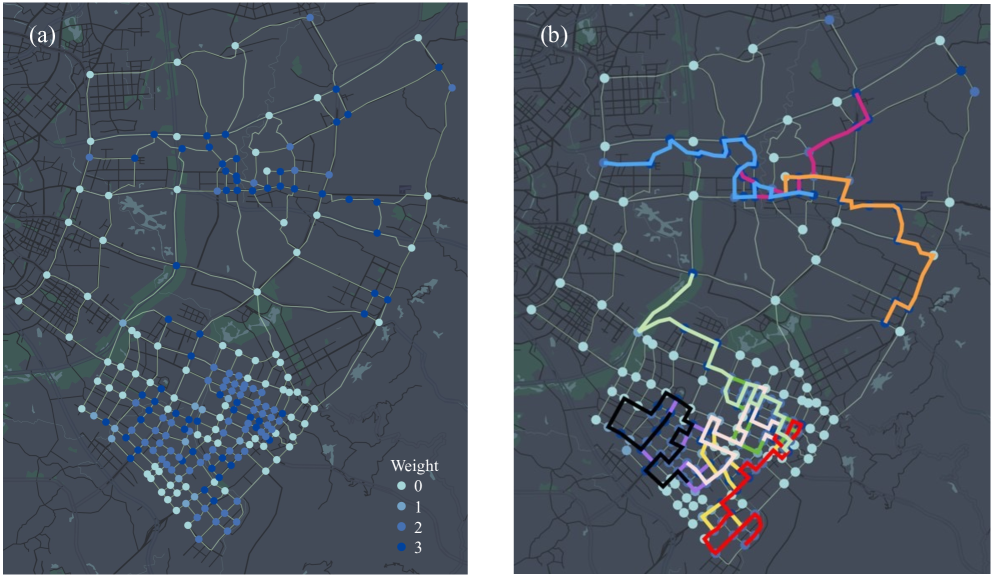
Figure 1: Demonstration of the ETOP solution: (a) A road network where the nodes are POIs with varying weights; (b) the 10 routes generated to visit these POIs.

Motivated by this, we propose the Extended Team Orienteering Problem (ETOP) by assuming that (1) each POI may be visited multiple times to accumulate scores; (2) the POIs have varying degrees of importance (weights); and (3) the score collected at each POI increases with the number of visits, but the marginal gain decreases. The aim of the ETOP is to determine a set of routes, each within a given time/distance budget and covering a subset of POIs, such that the total score is maximized. It is a nontrivial and necessary extension of the TOP. Furthermore, if the POIs are arcs instead of vertices, the ETOP can be applied to the route planning of anti-dust (road sprinkler) operation (Zhu et al.,, 2022) and road surface condition monitoring (Ali and Dyo,, 2017), which can be seen as an extension of the classical capacitated arc routing problem (CARP) (Golden and Wong,, 1981), with heterogeneous road link coverage.

We present a mathematical formulation of the ETOP as a nonlinear integer program, and two solution approaches: one based on the adaptive large neighborhood search (ALNS) algorithm (Windras Mara et al.,, 2022), the other being a bi-level matheuristic. Test results on complete graphs with different problem sizes show that: (1) both algorithms significantly outperform a greedy heuristic, with improvements ranging from 9.43% to 27.68%; and (2) while the ALNS-based algorithm slightly outperform the matheuristic in terms of solution optimality, its computational times are much higher, by 11 to 385 times. Finally, a real-world case study of mobile VOCs sensing on a road network is presented and formulated as ETOP on an incomplete graph. In this case, the ALNS is outperformed by matheuristic in terms of optimality as the destroy and repair operators yield limited perturbation of existing solutions when constrained by a road network (incomplete graph). Such a case study highlights the unique applicability of ETOP to certain real-world scenarios, as well as the effectiveness of the proposed algorithms in achieving a sensible solution.

The rest of this article is organized as follows. Section 2 articulate the ETOP with a mathematical formulation. Sections 3 and 4 present the ALNS and matheuristic solution approaches, respectively. A few discussions on model extensions are presented in Section 5. Section 6 presents extensive numerical and application studies. Finally, Section 7 presents some concluding remarks.

2 Problem Statement and Model Formulation

2.1 Preliminaries

We consider a geographic area with several points of interests (POIs), which are to be visited by a set of agents. The ETOP is articulated as follows.

Definition 2.1.

The Extended Team Orienteering Problem (ETOP) Given a set of POIs $I=\{1,...,n\}$. Each POI $i\in I$ is associated with a scoring function that depends on the POI itself as well as the number of times it is visited. Then, the ETOP is to determine $n_{K}$ routes, each to be executed by an agent within a fixed time or distance budget, such that the total score collected from visiting these POIs is maximized.

For each POI $i\in\{1,\ldots,n\}$, let $q_{i}\in\mathbb{Z}$ be the number of visits by all the agents. The scoring function, denoted $f_{i}(q_{i})$, needs to satisfy the following conditions:

1. $f_{i}(0)$=0, and $f_{i}(\cdot)$ is monotonically increasing;

2. The marginal gain of score is decreasing:

   $$f_{i}(q_{i,1}+1)-f_{i}(q_{i,1})>f_{i}(q_{i,2}+1)-f_{i}(q_{i,2})\qquad\forall 0\leq q_{i,1}<q_{i,2}$$

The first condition is straightforward. The second condition implies that when $i$ is visited many times, the extra score from one more visit is small. It is necessary to avoid over-concentration of visits at a few high-value POIs. The following function, which satisfies these conditions, will be used in this paper.

$$f(q_{i})=q_{i}^{\beta}\qquad\beta\in(0,1)$$ (2.1)

Finally, the objective of the ETOP is to maximize the following weighted sum:

$$f=\sum_{i\in I}w_{i}q_{i}^{\beta}$$ (2.2)

where the parameter $w_{i}$ is the weight of POI $i$. Intuitively, when $\beta\to 1$, the agents tend to visit high-weighting POIs more frequently; as $\beta\to 0$, their visits are more evenly distributed among all POIs. The parameters $w_{i}$’s and $\beta$ should be jointly determined based on the underlying application.

2.2 Mathematical Model

Table LABEL:tab_notations lists some key notations used in the model.

Table 1: Notations and symbols

Sets
$I$	Set of POIs;
$K$	Set of agents;
$N$	Set of vertices in the undirected graph $G$;
$A$	Set of arcs on the undirected graph $G$;
Parameters and constants
$n_{K}$	Number of agents;
$n$	Number of POIs;
$t_{ij}$	Travel time from vertex $i$ to vertex $j$;
$w_{i}$	The weight of POI $i$;
$\Delta$	The length of time or distance budget.
$\beta$	The parameter in the score function (2.1) that ensures diminishing marginal gain.
Auxiliary variables
$y_{i,k}$	Binary variable that equals $1$ if POI $i$ is visited by agent $k$;
$a_{i,k}$	The visiting time of POI $i$ by agent $k$;
$q_{i}$	The total number of times the POI $i$ is covered by the vehicles;
Decision variables
$x_{i,j,k}$	Binary variable that equals $1$ if agent $k$ travels directly from vertex $i$ to vertex $j$.

We consider a network represented as an undirected graph $G=(N,A)$, where $N$ is the set of vertices, and $A$ is the set of arcs. The arc set consists of two parts: those connecting any pair of POIs, as well as those connecting the starting/ending depots to the POIs: $A=\{(0,i)|i\in I\}\cup\{(i,j)|i,j\in I;t_{ij}\neq\inf\}\cup\{(j,n+1)|j\in I\}$. The full ETOP model is formulated as:

$$\max_{s=\{x_{i,j,k}:\,i,j\in I,k\in K\}}f(s)=\sum_{i\in I}w_{i}q_{i}^{\beta}$$ (2.3)

$$\sum_{i\in I}x_{0,i,k}=1 \forall k\in K$$ (2.4)

$$\sum_{i\in I}x_{i,n+1,k}=1 \forall k\in K$$ (2.5)

$$\sum_{(i,l)\in A}x_{i,l,k}=\sum_{(l,j)\in A}x_{l,j,k} \forall l\in I,\forall k\in K$$ (2.6)

$$\sum_{(i,j)\in A}x_{i,j,k}=y_{i,k} \forall i\in I,\forall k\in K$$ (2.7)

$$q_{i}=\sum_{k\in K}y_{i,k} \forall i\in I$$ (2.8)

$$a_{i,k}+t_{ij}-a_{j,k}\leq M(1-x_{i,j,k}) \forall i,j\in N,k\in K$$ (2.9)

$$a_{n+1}\leq\Delta$$ (2.10)

$$x_{i,j,k}\in\{0,1\} \forall i,j\in N,\forall k\in K$$ (2.11)

$$y_{i,k}\in\{0,1\} \forall i\in I,\forall k\in K$$ (2.12)

$$a_{i,k}\in\mathbb{R}_{+} \forall i\in I,\forall k\in K$$ (2.13)

The objective function (2.3) maximizes the weighted scores within time or distance budget $\Delta$. Constraints (2.4) and (2.5) ensure that each agent departs from the starting depot and return to the ending depot. Constraint (2.6) ensures flow conservation for each agent. Constraint (2.7) couples variables $x_{i,j,k}$ with indicator variable $y_{i,k}$. Constraint (2.8) calculates the total number of times the POI $i$ is visited by the agents. Constraint (2.9) acts as subtour elimination constraint (Miller et al.,, 1960). Constraint (2.10) ensure that the time or distance budget is not exceeded.

3 ALNS applied to the ETOP

This section describes a solution framework based on adaptive large neighborhood search (ALNS) for the ETOP. As summarized in Windras Mara et al., (2022), the ALNS has the following important parts: (1) initial solution $s_{0}$; (2) a set of destroy operators $\Omega^{-}=\{\Omega_{1}^{-},...,\Omega_{m}^{-}\}$; (3) a set of repair operators $\Omega^{+}=\{\Omega_{1}^{+},...,\Omega_{n}^{+}\}$; (4) adaptive mechanism; (5) acceptance criterion and (6) termination criterion. In each iteration of ALNS, a single destroy and a single repair operators are selected according to the adaptive mechanism. The destroy operator is first implemented to remove parts of a feasible solution $s$ and the resulting solution is stored in $s^{{}^{\prime}}$. The repair operator then re-inserts parts of elements to $s^{{}^{\prime}}$ so that $s^{{}^{\prime}}$ become a complete solution. Let $f(s),f(s^{{}^{\prime}}),f(s^{*})$ be the objective of the current solution, the newly obtained solution, and the best-known solution, respectively. At each iteration, an acceptance criterion is used to determine whether the newly obtained solution $s^{{}^{\prime}}$ is accepted as the current solution $s$. When the termination criterion is met, the algorithm outputs the optimal solution $s^{*}$. The framework of ALNS is shown in Algorithm 1.

Input: An initial solution $s_{0}$ (Section 3.1), set of destroy operators $\Omega^{-}$, set of repair operators $\Omega^{+}$.
  Output: Best-known solution $s^{*}$.

1:Initialize $s^{*}\leftarrow s_{0}$, $s^{{}^{\prime}}\leftarrow s_{0}$

2:while Termination Criterion (Section 3.6) not met do

3:     Select a destroy operator (Section 3.2) and a repair operator (Section 3.3) from $\Omega^{-}$ and $\Omega^{+}$ according to the adaptive mechanism.

4:     $s^{{}^{\prime}}\leftarrow repair(destroy(s))$

5:     if $s^{{}^{\prime}}$ is better than $s^{*}$ then

6:         $s^{*}\leftarrow s^{{}^{\prime}}$

7:         $s\leftarrow s^{{}^{\prime}}$

8:     end if

9:     if accept($s^{{}^{\prime}}$) (Section 3.5) then

10:         $s\leftarrow s^{{}^{\prime}}$

11:     end if

12:     Update the parameters of the adaptive mechanism

13:end while

Algorithm 1 (The framework of ALNS)

The rest of this section instantiates each step of the ALNS for solving the ETOP.

3.1 Initial Solution

The generation of an initial solution is non-trivial in the ETOP. We begin with the following definition.

Definition 3.1.

(Marginal gain) Given a POI $i\in I$ and the number of visits $q_{i}$ already made by the agents, the marginal gain refers to the additional score obtained from one more visit, namely $\eta_{i}=w_{i}\big{(}(q_{i}+1)^{\beta}-(q_{i})^{\beta}\big{)}$.

We adopt a greedy constructive heuristic algorithm to generate the routes of each agent in sequence. We begin with the POI $j\in I$ with the highest marginal gain as the starting location for the agent. The idea is to sequentially select the next POI $i^{*}$ that maximizes the reward efficiency $\psi_{ji}$ among all feasible POIs:

$$i^{*}=\mathop{\arg\max}\limits_{i}\psi_{ji}=\mathop{\arg\max}\limits_{i}\frac{\eta_{i}}{t_{ji}}$$ (3.14)

In prose, the reward efficiency refers to the score collected per unit spending of time (or distance). The pseudo-code for the generation of initial solution is shown in Algorithm 2.

Input: Number of agents $n_{K}$, the length of each time period $\Delta$, marginal gains $\{\eta_{i},i\in I\}$
  Output: Initial routing solutions $R_{0}$

1:for $v=1,...,n_{K}$ do

2:     Initialize $t=0$, list of candidate points $I_{temp}=I$;

3:     Set the starting point of vehicle $v$ as $s_{v}=\mathop{\arg\max}\limits_{i}\eta_{i}$;

4:     while $t<\Delta$ do

5:         Find the next visiting point $i^{*}=\mathop{\arg\max}\limits_{i}\psi{(i)}$;

6:         Add the point $i^{*}$ to the vehicle route $R_{0}^{v}$ and update the marginal gains $\{\eta_{i}|i\in I\}$;

7:         Update $t=t+t_{j,i^{*}}$;

8:         Set the current point is $j\leftarrow i^{*}$;

9:         Remove $j$ from the list of candidate points $I_{temp}$.

10:     end while

11:end for

Algorithm 2 (Generation of initial solution)

3.2 Destroy Operators

This section describes four removal heuristics: random removal, worst removal, related removal and route removal. All four heuristics take the current solution $s$ as input. The output of the heuristic is a temporary solution $s_{temp}^{{}^{\prime}}$ after applying the destroy operator, which removes some points from the current solution $s$.

3.2.1 Random removal

In the random removal heuristic, we randomly remove $m\%$ of the points (any decimals will be rounded to the nearest integer) from the route of each agent using a uniform probability distribution.

3.2.2 Worst removal

As proposed in Ropke and Pisinger, (2006), the worst removal heuristic removes points with the aim of obtaining most savings. For the ETOP, we need to consider the trade-off between collecting scores and the time/distance required. Specifically, we aim to remove the POIs that have limited impact on the total score, while resulting in the most time/distance savings.

Let $\mathcal{V}$ be the set of visited POIs in the current solution $s$. Given a POI $i\in\mathcal{V}$, we use $f(s)$ to represent the score of the current solution $s$, and $T(s)$ to represent the total time/distance used by all agents in the current solution $s$. Next, we define the score lost by removing $i$ from the current solution $s$ as $r(i,s)=f(s)-f_{-i}(s)$, and the time/distance saved as $t(i,s)=T(s)-T_{-i}(s)$. We define the value of each POI in the current solution $s$ as $value(i,s)$:

$$value(i,s)=\frac{r(i,s)}{t(i,s)}$$ (3.15)

Building on such a notion, this operator iteratively removes POIs with relatively low values. Following Ropke and Pisinger, (2006), we introduce random factors to avoid situations where the same points are removed over and over again. In addition, randomization is applied in a way that favors the selection of POIs with lower values. The pseudo-code for the worst removal heuristic is shown in Algorithm 3.

Input: A current solution $s$, proportion $m$% of point removal, parameter $p>0$
  Output: Temporary solution $s_{temp}^{{}^{\prime}}$ after destroy operator

1:Calculate the number of POIs to be removed based on $m$%, denoted as $n_{p}$;

2:for $n=1,...,n_{p}$ do

3:     List of all visited POIs in the current solution $s$, denoted as $\mathscr{V}$;

4:     $\mathscr{V}_{new}$ = Sorted list of $\mathscr{V}$ in an increasing order of $value(i,s)$, $i\in\mathcal{V}$;

5:     Draw a random number $y$ from the uniform distribution $U(0,1)$;

6:     Let $x$ be the $\lfloor y^{p}|\mathscr{V}|\rfloor$-th element in the ordered set $\mathscr{V}_{new}$ ($\lfloor\cdot\rfloor$ is the floor operator);

7:     Remove point $x$ from the current solution $s$.

8:end for

Algorithm 3 (Worst removal)

3.2.3 Related removal

The purpose of the related removal heuristic is to remove a set of points that, in some way, are closely related and hence easy to interchange among different routes during repairs (Pisinger and Ropke,, 2007). For the ETOP, we remove some adjacent POIs, with the understanding that points closer to each other are more likely to be interchanged. Specifically, we first randomly select a POI $o\in I$ as the center point, and then remove the $m\%$ points closest to $o$ in the current solution $s$.

3.2.4 Route removal

This operator is commonly used in the vehicle routing problem (Demir et al.,, 2012). For the ETOP, the operator randomly removes $\left[n_{K}\times m\%\right]$ of the routes from the solution $s$, where $n_{K}$ is the number of routes ($\left[\cdot\right]$ is the rounding operator).

3.3 Repair Operators

This section describes some insertion heuristics: greedy insertion and (k)-regret insertion. Insertion heuristics are typically divided into two categories: sequential and parallel. The difference between the two is that the former builds one route at a time while the latter constructs several routes simultaneously (Potvin and Rousseau,, 1993). The insertion heuristics adopted in this paper are all parallel, which will be used to repair the temporary solution $s_{temp}^{{}^{\prime}}$ following the destroy operator. The output of the insertion heuristic is a new feasible solution $s^{{}^{\prime}}$.

3.3.1 Greedy insertion

Definition 3.2.

(Minimum-cost position) Given a POI $i\in I$ and a route $R_{k}$, there are $|R_{k}|+1$ possible insertion positions for this POI. Let $\Delta t_{ik}(m)$ be the extra time/distance incurred by inserting $i$ into the $m$-th position of $R_{k}$. We define the minimum-cost position to be $m_{ik}^{*}=\mathop{\arg\min}\limits_{m=\{1,...,|R_{k}|+1\}}\Delta t_{ik}(m)$ and the minimum cost as $\Delta t_{ik}(m_{ik}^{*})$.

Let $\Delta r_{i,k}$ be the increased score after inserting point $i$ into the route of agent $k$ at the minimum-cost position. If the POI $i$ cannot insert to the route of agent $k$, we set $\Delta r_{i,k}=0$

Definition 3.3.

Similar to the reward efficiency defined in (3.14), the reward efficiency of inserting point $i$ is defined as the extra score collected per unit time/distance required to accommodate such insertion:

$$\Psi_{i,k}\doteq{\Delta r_{i,k}\over\Delta t_{ik}(m_{ik}^{*})}$$

Then, we define the maximum insertion-value of $i$ to be

$$v(i)\doteq\max_{k\in K}\Psi_{i,k}$$ (3.16)

The greedy insertion operator iteratively selects and inserts a candidate POI $i$ that has the maximum insertion-value $v(i)$. This process continues until no more POIs can be inserted into any route.

3.3.2 (k)-Regret insertion

The regret heuristic tries to improve upon the greedy heuristic by incorporating look-ahead information when selecting the point for insertion (Ropke and Pisinger,, 2006). In prose, the algorithm performs the insertion that will be most regretted if it is not done now. Recalling the notions from Section 3.3.1:

$$\Delta v_{ik}(m)=\frac{\Delta r_{i,k}}{\Delta t_{ik}(m)}\qquad\forall i\in I,\quad k\in K,\quad m=\{1,...,|R_{k}|+1\}$$ (3.17)

We sort the list $\big{\{}\Delta v_{ik}(m):i\in I,k\in K,1\leq m\leq|R_{k}|+1\big{\}}$ in descending order to obtain $\big{\{}\Delta v^{(n)}_{ik}(m):i\in I,k\in K,1\leq m\leq|R_{k}|+1\}\big{\}}$ where $n$ indexes the ordered elements in the list. Then, the $k$-regret heuristic chooses to insert the POI that maximizes $c_{k}^{*}$ in each step.

$$c_{k}^{*}=\sum_{j=1}^{k}(\Delta f_{ik}^{j}(m)-\Delta f_{ik}^{1}(m))$$ (3.18)

where $c_{k}^{*}$ is the $k$-regret value. This process continues until no POI can be inserted into any route.

3.4 Adaptive Mechanism

We defined, in Section 3.2, four destroy operators (random, worst, related, and route removal), and in Section 3.3 a class of repair operators (greedy insertion, $k$-regret). This section explains a strategy to adaptively select the destroy and repair operators at each iteration of ALNS.

We assign weights to different opertors and implement the classical roulette wheel mechanism (Ropke and Pisinger,, 2006). If we have $L$ operations with weights $\mu_{l}$, $l\in\{1,2,...,L\}$, we select operator $l$ with probability $p_{l}$ given as:

$$p_{l}=\frac{\mu_{l}}{\sum_{l=1}^{L}\mu_{l}}$$ (3.19)

Initially, we set the same weight for each operator. Then, we continuously update the weight by keeping track of a score for each operator, which measures how well the heuristic has been performing recently. Operators with higher scores have a higher probability of being selected during the iteration. The entire search is divided into a number of segments, indexed by $h$. A segment contains a few iterations of the ALNS, hereafter defined to be $\delta$ iterations. The score of all operators is set to zero at the start of each segment. The score of the operators are updated according to the following rules:

• if the score of the new solution is better than the best-known solution, the operator score increases by $\sigma_{1}$;

• if the score of the new solution is worse than the best-known solution, but better than the current solution, the operator score increases by $\sigma_{2}$;

• if the score of the new solution is worse than the current solution, but is accepted, the operator score increases by $\sigma_{3}$;

• if the new solution is not accepted, the operator score increases by $\sigma_{4}$.

It is reasonable to set $\sigma_{1}>\sigma_{2}>\sigma_{3}>\sigma_{4}$. At the end of each segment we calculate new weights using the recorded scores. Let $\mu_{l,h}$ be the weight of operator $l$ used in segment $h$, and the probability $p_{l,h}$ is calculated according to (3.19). At the end of each segment $h$ we update the weight for operator $l$ to be used in segment $h+1$ as follows:

$$\mu_{l,h+1}=\mu_{l,h}(1-\varepsilon)+\varepsilon\frac{\pi_{l,h}}{\theta_{l,h}}$$ (3.20)

where $\pi_{l,h}$ is the score of operator $l$ obtained during the last segment and $\theta_{l,h}$ is the number of times operator $l$ was used during the last segment. The reaction factor $\varepsilon$ controls how quickly the weight adjustment algorithm reacts to changes in the effectiveness of the operators.

3.5 Acceptance Criterion

A simulated annealing framework is used to decide whether to accept the newly obtained solution $s^{{}^{\prime}}$ given the current solution $s$. If the objective value $f(s^{{}^{\prime}})>f(s)$, then $s^{{}^{\prime}}$ is accepted as the current solution. Otherwise, the probability of $s^{{}^{\prime}}$ being accepted is $P(s\leftarrow s^{{}^{\prime}})$.

$$P(s\leftarrow s^{{}^{\prime}})=\exp\left\{\frac{f(s^{{}^{\prime}})-f(s)}{T}\right\}$$ (3.21)

where $T>0$ is the temperature, which begins with $T_{\text{max}}$ and decreases at every iteration according to $T=T\cdot c$, where $c\in(0,1)$ is the cooling rate. When $T$ is below $t_{\text{min}}$, take reheating measures and set $T$ to $T_{\text{max}}$.

3.6 Termination Criterion

The algorithm stops after: (1) a maximum number of iterations $N_{1}^{\text{max}}$; or (2) a certain number of non-improving iterations $N_{2}^{\text{max}}$.

4 A matheuristic method for the ETOP

This section proposes a matheuristic method to solve the ETOP based on a bi-level structure. The master (upper) problem is a route selection model and the sub (lower) problem generates a new route. The matheuristic iteratively adds new routes that may improve the score to the candidate list of the master problem until the termination criterion is met. The pseudo-code of the matheuristic method is shown in Algorithm 4.

Step 1: Initial candidate route list $R$ by Algorithm 2; the non-improving iterations $\delta=0$; the best objective value $f=0$; termination parameter $N_{0}^{\text{max}}$.
Step 2: Solve the master problem in Section 4.1 with the candidate route set $R$, and obtain the route of each agent. Record the current objective value as $f^{*}$.
Step 3: Update the marginal gain of each POI based on the result of Step 2.
Step 4: Obtain a new candidate route by solving the sub problem in Section 4.2 and add it to the candidate route list $R$.
Step 5: If $f^{*}>f$, update the best objective value $f=f^{*}$ and reset $\delta=0$, otherwise, $\delta=\delta+1$.
Step 6: If $\delta<N_{0}^{\text{max}}$, go to Step 2; otherwise, terminate the algorithm.

Algorithm 4 (The matheuristic method)

4.1 The master problem

The master problem is a route selection model. Let $R$ be the set of candidate routes to be selected, and $\lambda_{kr}$ be a binary variable taking the value 1 if agent $k$ selects the route $r$. Let $a_{ir}$ be a binary parameters taking the value 1 if the route $r$ visits POI $i$. Then, $q_{i}$ is an auxiliary variable representing the number of visits of POI $i$.

$$\max_{\{\lambda_{kr}:\,k\in K,r\in R\}}f=\sum_{i\in I}w_{i}q_{i}^{\beta}$$ (4.22)

$$\sum_{r\in R}\sum_{k\in K}\lambda_{kr}a_{ir}=q_{i} \forall i\in I$$ (4.23)

$$\sum_{r\in R}\lambda_{kr}=1 \forall k\in K$$ (4.24)

$$\sum_{r\in R}\sum_{k\in K}\lambda_{kr}\leq n_{K}$$ (4.25)

$$\lambda_{kr}\in\{0,1\} \forall k\in K,\forall r\in R$$ (4.26)

The objective function (4.22) maximizes the weighted sum of scores. Constraints (4.23) calculate the total number of visits of POI $i$ by the agents. Constraints (4.24) ensure that each agent must choose exactly one route. Constraint (4.25) ensure that the number of selected routes cannot exceed the number of agents. The master problem is a knapsack problem, which can be solved directly by commercial solver.

4.2 The sub-problem

The sub problem aims to generate a new route $r^{*}$ which may improve the score, and add it to the set $R$ of candidate routes for the master problem. Let $x_{i,j}$ be a binary variable taking the value 1 if the new route directly connects vertex $i$ to vertex $j$, $y_{i}$ be a binary variable taking the value 1 if POI $i$ is visited by the new route. Let $z_{i}$ be the order in which POI $i$ is visited in the new route, and we set $z_{0}=0$ and $z_{n+1}=n+1$ (where $0$ and $n+1$ are deemed the starting and ending depots). Finally, $\eta_{i}$ denotes the marginal gain of POI $i$.

$$\max_{x_{i,j}}\sum_{i\in I}\eta_{i}y_{i}$$ (4.27)

$$\sum_{i\in I}x_{0,i}=1$$ (4.28)

$$\sum_{i\in I}x_{i,n+1}=1$$ (4.29)

$$\sum_{(i,l)\in A}x_{i,l}=\sum_{(l,j)\in A}x_{l,j} \forall l\in I$$ (4.30)

$$\sum_{(i,j)\in A}x_{i,j}=y_{i} \forall i\in I$$ (4.31)

$$\sum_{(i,j)\in A}t_{ij}x_{i,j}\leq\Delta$$ (4.32)

$$z_{i}-z_{j}+1\leq n(1-x_{i,j}) \forall(i,j)\in A$$ (4.33)

$$1\leq z_{i}\leq n \forall i\in I$$ (4.34)

$$x_{i,j}\in\{0,1\} \forall(i,j)\in A$$ (4.35)

$$y_{i}\in\{0,1\} \forall i\in I$$ (4.36)

The objective function (4.27) maximizes the total marginal gain collected by the new route. Constraints (4.28) and (4.28) ensure that the route starts from node $0$ and ends with node $n+1$ (i.e. the depots). Constraints (4.30) expresses flow conservation. Constraints (4.31) relates variables $x_{i,j}$ to the indicator variable $y_{i}$. Constraint (4.32) ensure that the time or distance budget is not exceed. Constraints (4.33) and (4.34) act as sub-tour elimination constraints (Miller et al.,, 1960). We note that the sub problem is an orienteering problem, which is solved by the heuristic algorithm (Chao et al., 1996a, ) in this paper.

5 Discussion and extension

This section provides some discussion on the ETOP when modeling various real-world problems.

5.1 Completeness of graphs

The ETOP proposed in this paper takes as input the POI set $I$, their weights in the objective $\{w_{i}:\,i\in I\}$, and the adjacency matrix. In practice, the adjacency matrix is replaced by the travel time (or distance) matrix $\{t_{ij}:\,i,j\in I\}$, where $t_{ij}$ denotes the travel time (or distance) from vertex $i$ to $j$.

• In application scenarios like UAV routing, the spatial domain of the problem is a subset of a Euclidean space, in which any two vertices are directly connected. In this case, any element of the adjacency matrix $t_{ij}$ is a finite number. In other words, all the POIs can be seen as vertices in a complete graph.

• In application scenarios like car routing, the spatial domain is a road network represented as a directed graph $G(\mathcal{V},\,\mathcal{A})$, where $\mathcal{V}$ is the set of vertices and $\mathcal{A}$ is the set of arcs, we set $t_{ij}=\infty$ whenever the arc $(i,j)\notin\mathcal{A}$. In other words, road networks can be seen as incomplete graphs.

Not only is the completeness of graphs linked to different application domains (e.g. UAV routing or car routing), it also impacts the effectiveness of the ALNS as we later demonstrate in Sections 6.3 and 6.4.

5.2 Arcs as POIs

In some applications based on road networks, the scores are collected on arcs instead of nodes. Examples include road surface sprinkling (aiming at reducing fugitive dust), or road roughness monitoring (for regular maintenance and repair). Such tasks need to be repeatedly performed, and the weights of these arcs are heterogeneous. These problems fall within the purview of ETOP because one can simply augment the original network with artificial nodes (with scores assigned) in the middle of relevant arcs. For example, if arc $(i,j)\in\mathcal{A}$ carries scores, we insert a node $k$ to form two new arcs $(i,k)$ and $(k,j)$, and set $t_{ik}=t_{kj}={1\over 2}t_{ij}$. Then, the weight and score of arc $(i,j)$ in the original network are transferred to node $k$ in the augmented network. Such a simple technique converts arc-based ETOP to node-based ETOP, which can be solved with the proposed algorithms.

6 Computational studies

All the computational performances reported below are based on a Microsoft Windows 10 platform with Intel Core i9 - 3.60GHz and 16 GB RAM, using Python 3.8 and Gurobi 9.1.2.

6.1 Model and algorithm parameters

In ALNS, the destroy operators are parameterized by $m$, which will be determined through sensitivity analysis in Section 6.2.2. The insertion heuristics in the repair operators are parameter free. The weight adjustment algorithm is parameterized by $\sigma_{1}$, $\sigma_{2}$, $\sigma_{3}$, $\sigma_{4}$ and learning rate $\varepsilon$. We set $(\sigma_{1}$, $\sigma_{2}$, $\sigma_{3}$, $\sigma_{4})=(20,10,3,0)$; the parameter $\varepsilon$ will be determined through the sensitivity analysis in Section 6.2.2. To manage the acceptance criterion we use three parameters, $T_{\text{max}}$, $t_{\text{min}}$ and $c$. The start temperature $T_{\text{max}}$ is determined based on the value of the initial solution $f(s_{0})$ and the formula is $T_{\text{max}}=0.05\times\frac{f(s_{0})}{\ln(2)}$, which allows for a 50% probability that non-improving solutions generated at the initial solution temperature is accepted. In addition, we set $t_{\text{min}}=0.1$ and $c=0.95$. We also need to determine $N_{1}^{\text{max}}$ and $N_{2}^{\text{max}}$ that govern algorithm termination. We set $N_{1}^{\text{max}}$ to a large number 2000, and mainly rely on $N_{2}^{\text{max}}$ to terminate the algorithm. The value of parameter $N_{2}^{\text{max}}$ will be determined through sensitivity analysis in Section 6.2.2.

In the matheuristic method, only parameter $N_{0}^{\text{max}}$ needs to be determined and the sensitivity analysis results are shown in Section 6.2.3.

6.2 Sensitivity analysis of key parameters

6.2.1 Test datasets (complete graphs)

This section analyzes the impact of some key parameters or operators on the model performance, and subsequently chooses their appropriate values. For this purpose, we consider three test datasets with randomly generated locations and weights of POIs, as shown in Figure 2. Note that in this case, the travel times $t_{ij}$ are directly calculated as the Euclidean distance between two points. In other words, those POIs depicted in Figure 2 are vertices in complete graphs.

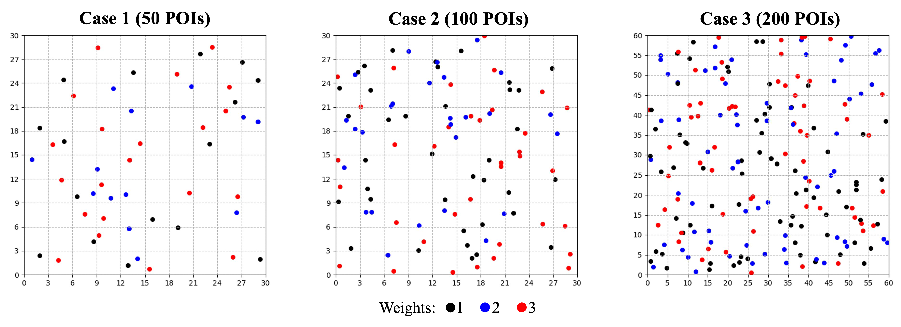
Figure 2: Three test datasets with randomly generated locations and weights of POIs.

6.2.2 ALNS parameters

The sensitivity analysis of parameters $m$, $\varepsilon$ and $N_{2}^{\text{max}}$ is conducted with the following constants ($n_{K}$, $\Delta$, $\beta$)=(4, 30, 0.5). We provide detailed explanation of these parameters and their test values in Table 2. We tune one parameter at a time by conducting 10 independent runs, while fixing the other parameters. The objective values and the CPU time are averaged and are shown in Figure 3.

Table 2: Parameters summarization in Algorithm ALNS.

Parameter	Description	Values
$m$	Percentage of points removed in the destroy operators.	$0.1:0.1:0.5$
$\varepsilon$	The reaction factor controls how quickly the weight adjustment algorithm reacts to changes in the effectiveness of the operators.	$0.3:0.1:0.7$
$N_{2}^{\text{max}}$	Number of non-improving iterations.	$100:50:350$

The results with regard to $m$ are shown in the first column of 3. For all three test cases, it is evident that the CPU times increase with $m$. Regarding the objective value, Cases 1 & 2 show similar increasing trends while Case 3 shows a non-monotone profile due to the size and complexity of the problem. All cases considered, we set $m=0.4$ (40%) for subsequent calculations.

The results with regard to $\varepsilon$ are shown in the second column of Figure 3. In all three cases, the objective value displays concave trends with the optimal value of $\varepsilon$ around $0.5$. The trends of CPT times are less obvious. We set $\varepsilon=0.5$ in the following computational experiments.

The results with regard to $N_{2}^{\text{max}}$ are shown in the third column of Figure 3. It is seen that, in all three cases, the objective values and CPU times increase with $N_{2}^{\text{max}}$ with only minor exceptions. We set $N_{2}^{\text{max}}=300$ in the following computational experiments.

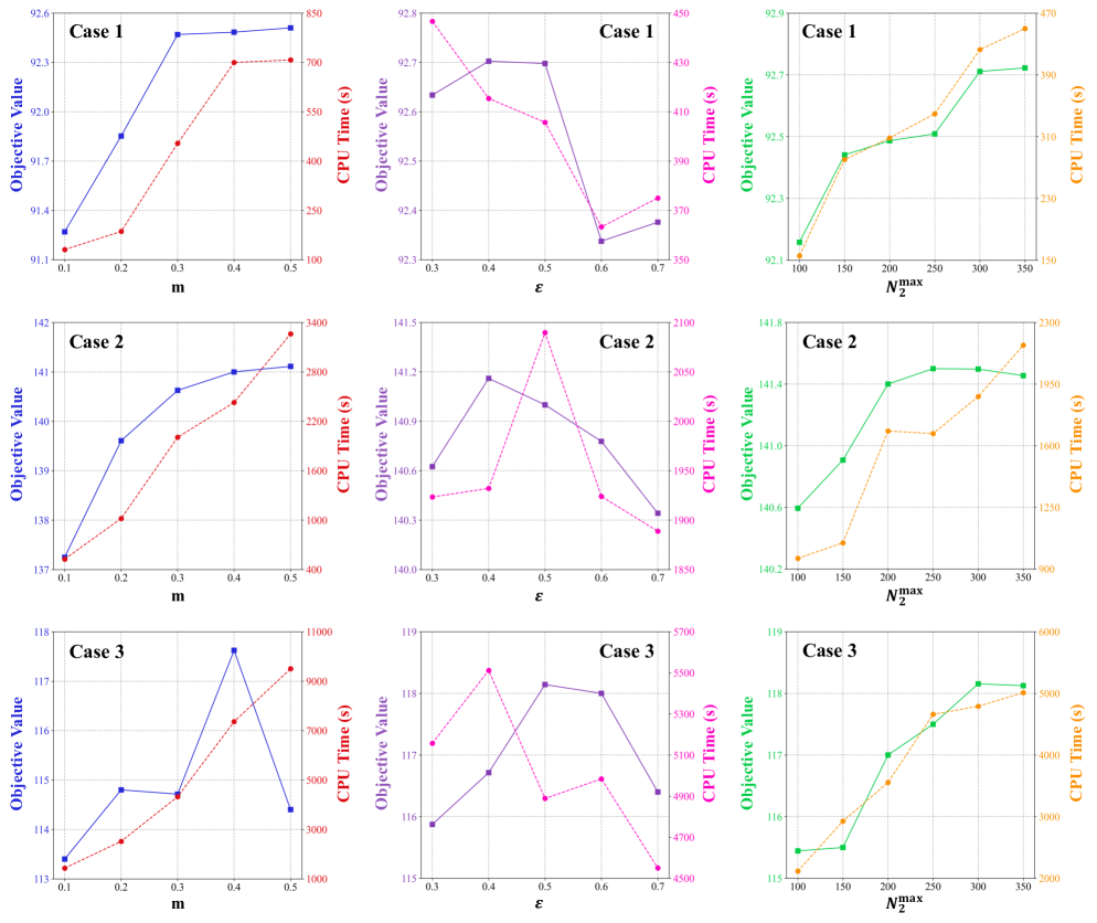
Figure 3: Average objective values and CPU times with different values of $m$, $\varepsilon$ and $N_{2}^{\text{max}}$.

6.2.3 Matheuristic parameters

The sensitivity analysis of the parameter $N_{0}^{\text{max}}$ is conducted with the following constants ($n_{K}$, $\Delta$, $\beta$)=(4, 30, 0.5). The values tested for the number of non-improving iterations $N_{0}^{\text{max}}$ are $\{50,100,150,200,250\}$. The results averaged from 10 independent runs are shown in Figure 4. The CPU times all increase with the threshold value $N_{0}^{\text{max}}$, as expected. In addition, the effect on the objective value is limited past $100$. Therefore, we set $N_{0}^{\text{max}}=100$ in the following computational experiments.

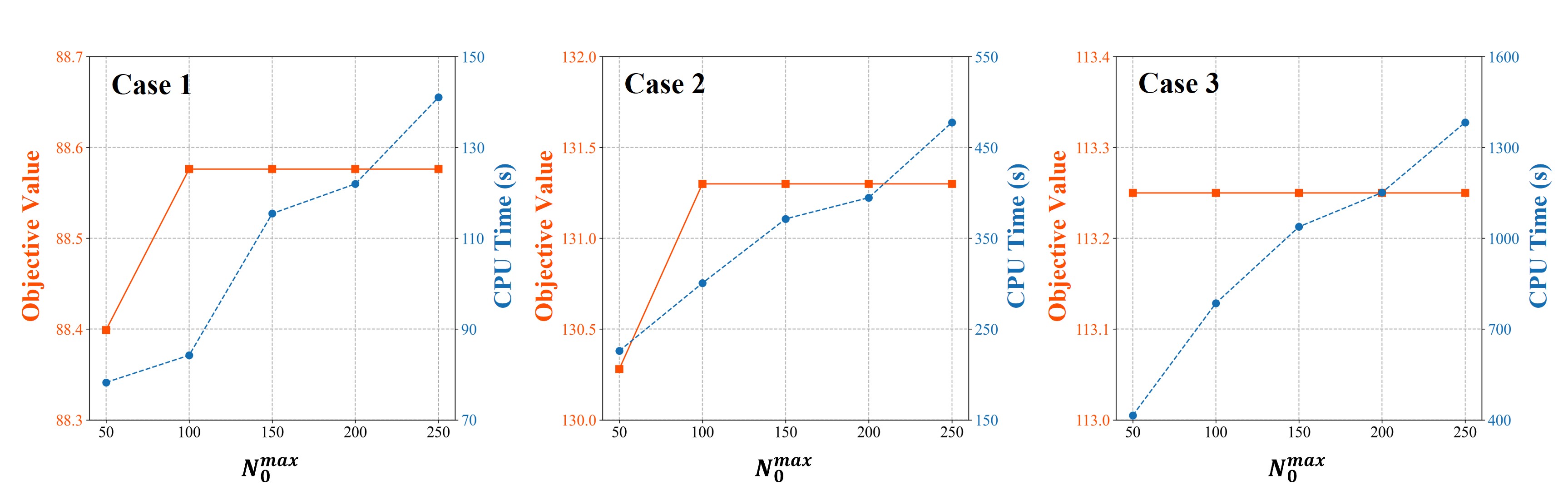
Figure 4: Average objective values and CPU times with different values of $N_{0}^{\text{max}}$.

6.2.4 Adaptive weights of the operators in ALNS

The ALNS algorithm employed in this paper considers four removal operators (random removal, worst removal, related removal and route removal) and five repair operators (greedy insertion, 2-regret insertion, 3-regret insertion, 4-regret insertion, 5-regret insertion). Here, we consider Case 3 with the constants $(n_{K}$, $\Delta$, $\beta)=(4,30,0.5)$, and show in Figure 5 the weights of these operators as they evolve over iterations of the ALNS.

We find that: (1) All the plots show decreasing trends because of the simulated annealing acceptance criteria; (2) For the destroy operators, the random and worst removal operators are selected over related and route removal by the adaptive mechanism; (3) The greedy and 5-regret insertion operators show better performance than the others.

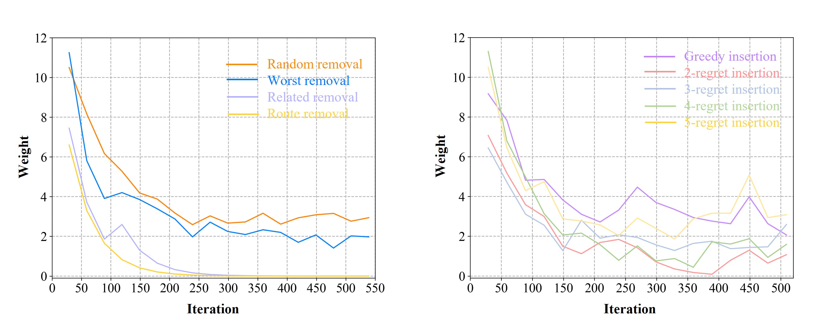
Figure 5: The weights of the destroy (left) and repair (right) operators as they evolve over iterations of the ALNS.

6.3 Algorithm performance

In this section, we compare the solution optimality and CPU times of greedy algorithm (Algorithm 2), ALNS and matheuristic on the three datasets described in Section 6.2.1. The test results under different $n_{K}$ (number of routes) are shown in Figure 6 and Table LABEL:tab_benchmark. It is shown that:

• The matheuristic and ALNS significantly outperform the greedy algorithm in solution optimality, with improvements ranging from 9.43% to 27.68%;

• Such improvements are less pronounced for larger $n_{K}$ (number of routes), because of (i) the diminishing marginal gain by design; (2) relatively high saturation of agent routes;

• Although the ALNS slightly outperform the matheuristic, the latter is much more computationally efficient, by a factor of $10^{2}$ for larger instances $n_{K}\geq 12$.

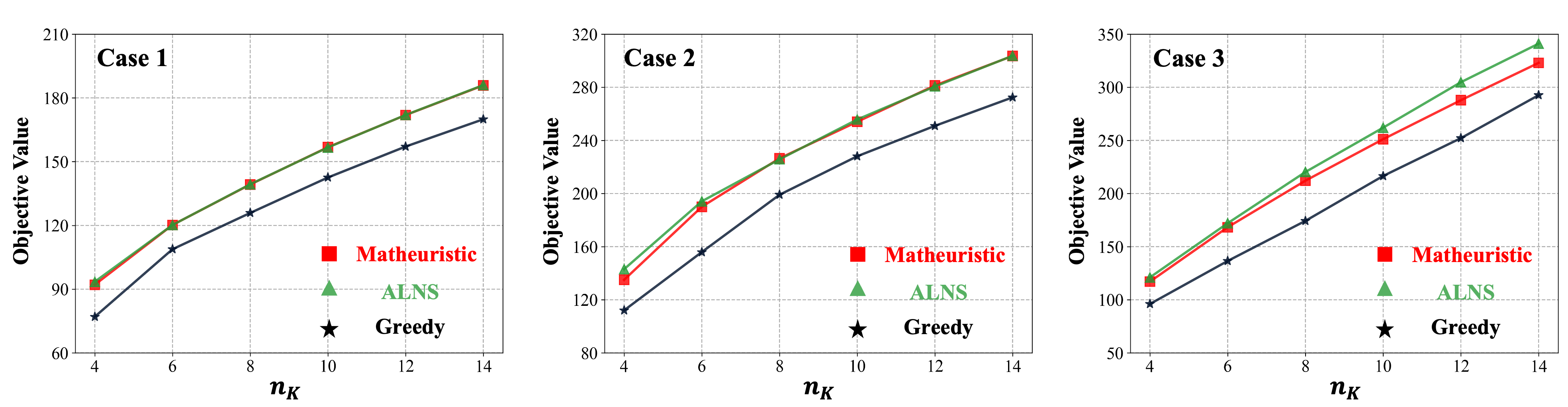
Figure 6: Objective values in three test cases with different values of $n_{K}$.

Table 3: Comparison of objective values and CPU times among greedy algorithm, matheuristic and ALNS. The ‘Increase’ column represents improvements over the greedy algorithm; the numbers in the parentheses in the ALNS-CPU column are computed as ALNS-CPU/Matheuristic-CPU.

	$n_{K}$	Greedy	Matheuristic			ALNS
		Obj.	Obj.	CPU(s)	Increase	Obj.	CPU(s)	Increase
Case 1	4	77.0	92.1	45	19.57%	93.5	777 (17)	21.40%
50 POIs	6	108.8	120.2	56	10.49%	120.2	848 (15)	10.49%
$\Delta=30$	8	125.9	139.2	63	10.63%	139.4	2326 (37)	10.72%
	10	142.5	156.8	55	10.01%	156.7	4867 (88)	9.92%
	12	157.1	171.9	46	9.43%	172.0	6770 (147)	9.46%
	14	170.0	185.9	43	9.39%	186.0	10925 (254)	9.47%
Case 2	4	112.0	135.0	308	20.54%	143.0	3504 (11)	27.68%
100 POIs	6	155.9	190.0	420	21.88%	194.1	7344 (17)	24.52%
$\Delta=30$	8	199.1	226.5	363	13.78%	225.7	9809 (27)	13.40%
	10	228.1	254.0	293	11.39%	255.7	18006 (61)	12.13%
	12	251.0	281.4	259	12.12%	280.6	34408 (133)	11.81%
	14	272.4	303.6	246	11.45%	303.8	40550 (165)	11.50%
Case 3	4	96.0	117.0	261	21.88%	121.0	11841 (45)	26.04%
200 POIs	6	136.5	168.2	290	23.26%	172.0	12510 (43)	26.02%
$\Delta=30$	8	174.2	212.1	317	21.71%	220.2	31293 (99)	26.40%
	10	216.5	251.1	497	15.98%	262.0	47984 (97)	21.00%
	12	252.1	287.9	307	14.17%	304.8	118219 (385)	20.89%
	14	292.6	323.0	477	10.39%	341.1	126867 (266)	16.57%

Figure 7 provides a visualization of the ETOP solution for Case 1, with four routes and different distance budget $\Delta$. It can be seen that, even for a small-scale problem, the solution displays some complexity, especially for larger $\Delta$ where the routes have considerable overlap. Moreover, such overlap took place at high-value nodes, which reflects the effectiveness of our proposed algorithms. Such solutions cannot be obtained via conventional TOPs or their variants.

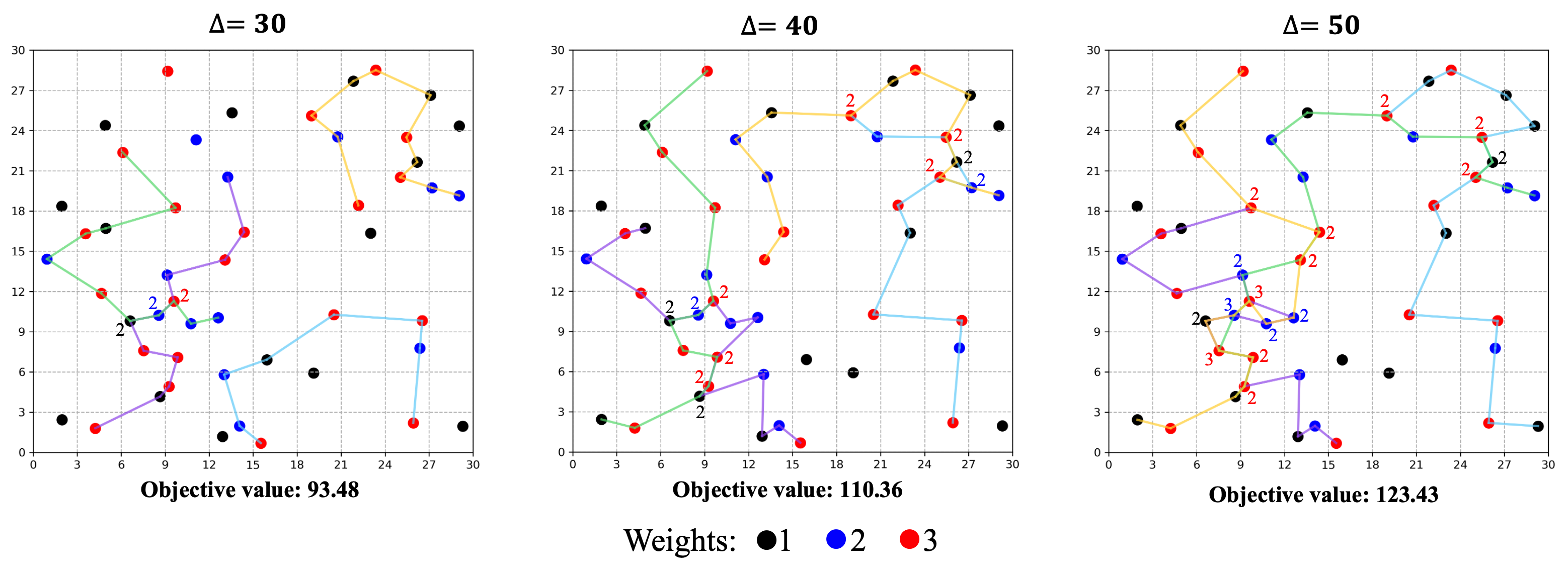
Figure 7: Solution visualization of Case 1 with four routes. $\Delta$ is the distance budget for each route. Nodes visited more than once are labeled with the number of visits.

6.4 Real-world case study (incomplete graphs)

The ETOP is demonstrated in a real-world case of Volatile Organic Compounds (VOCs) monitoring in the Longquanyi District, Chengdu, China. VOCs include a wide variety of chemicals, some of which have adverse health effects and act as catalyst of processes that form PM_2.5 and O₃ (Mishra et al.,, 2023, Yang et al.,, 2020). VOCs are emitted from the manufacturing activities from 141 factories in Longquanyi, and a single VOCs sensing vehicle, operated by local environmental protection agency, needs to perform regular monitoring tasks of the area by moving along designated routes.

The 141 factories are categorized into four class: A, B, C and D, where class A has the lowest sensing priority and D has the highest; see Figure 8(a). Based on the locations of these factories and their relative positions to the road network, their sensing priorities are transformed into the weights of the network nodes, which are treated as the POIs in our model; see Figure 8(b).

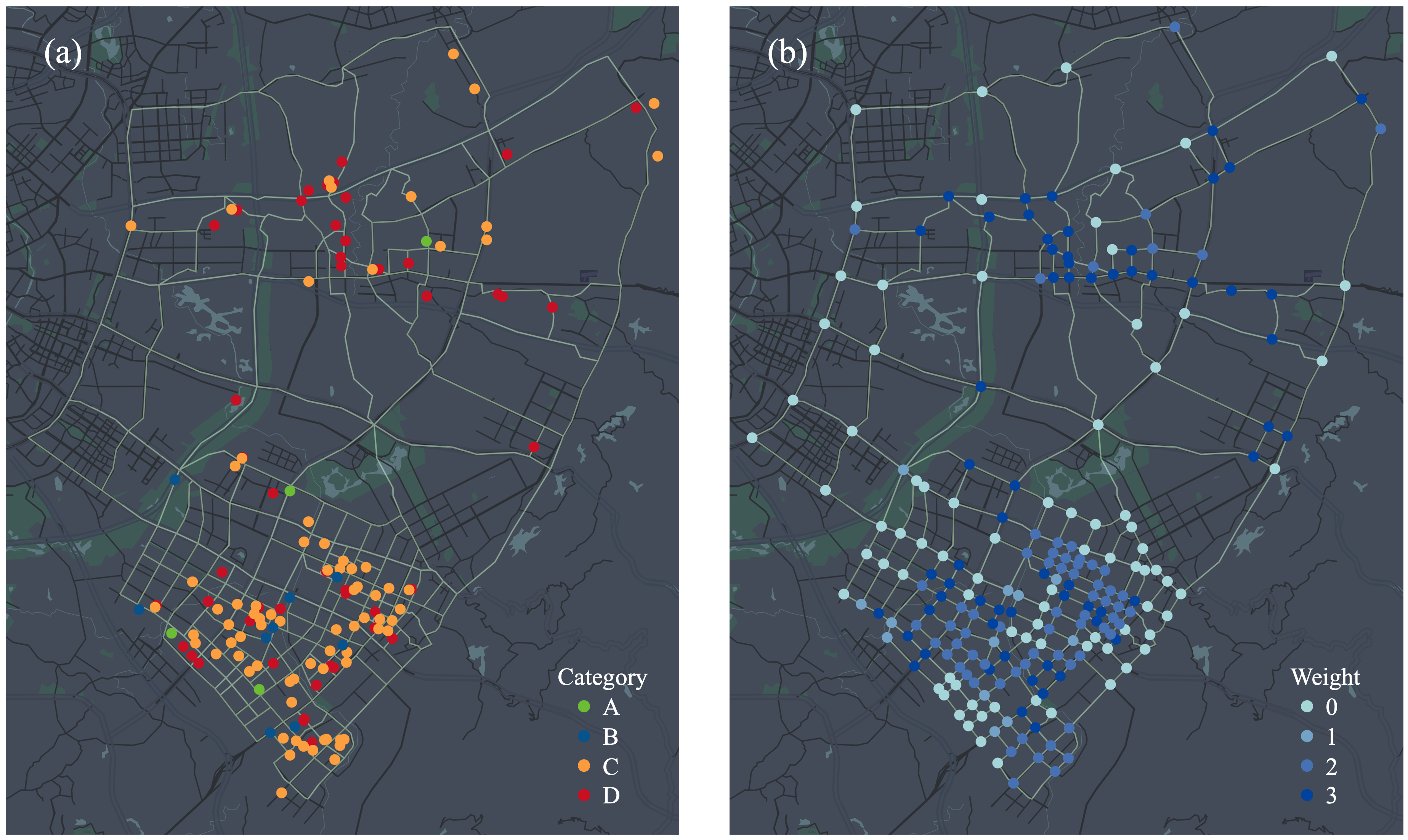
Figure 8: (a): Road network and distribution of factories of Longquanyi District, Chengdu. (b): The sensing weights of all the road network nodes.

We begin by comparing the performance of the matheuristic and the ALNS in Table 4. The computational efficiency of the former is significantly higher, which agrees with Table LABEL:tab_benchmark. Interestingly, unlike our previous finding in Figure 6, the ALNS is outperformed by the matheuristic in terms of solution optimality. The reason is that the destroy and repair operations used in the ALNS are constrained by the road network, leading to limited number of viable perturbations of a routing solution, which is different from the situation on a complete graph (Figure 2).

Table 4: Comparison of objective values and CPU times between matheuristic and ALNS. The relative increases of the objective values of the matheuristic are shown in the parentheses.

$n_{K}$	Matheuristic		ALNS
	Obj.	CPU(s)	Obj.	CPU(s)
4	239.4 (4.86%)	1000	228.3	2050
6	315.1 (5.63%)	1250	298.3	3622
8	374.9 (3.19%)	1404	363.3	5041
10	422.5 (2.42%)	2463	412.5	6268
12	465.6 (4.37%)	3007	446.1	9207
14	514.3 (6.52%)	3590	482.8	13261

Finally, to assess the validity of the solution in a mobile sensing context, we assume that the sensing vehicle needs to perform two routes per day, each within a distance budget of 20 km. Therefore, 10 routes need to be generated for a week’s (5 working days) monitoring task. This is formulated as an ETOP and solved by the ALNS and matheuristic, whose performance is compared in Figure 9(a). Figure 9(b) shows the 10 routes generated by the matheuristic. In this solution, 7 routes are located in the southern part of the area where the majority of the POIs are located. Moreover, many of the high-value POIs (with higher weights) are covered by multiple routes, which means those factories with higher sensing priority are more frequently visited, which is a desired feature of the routing plan.

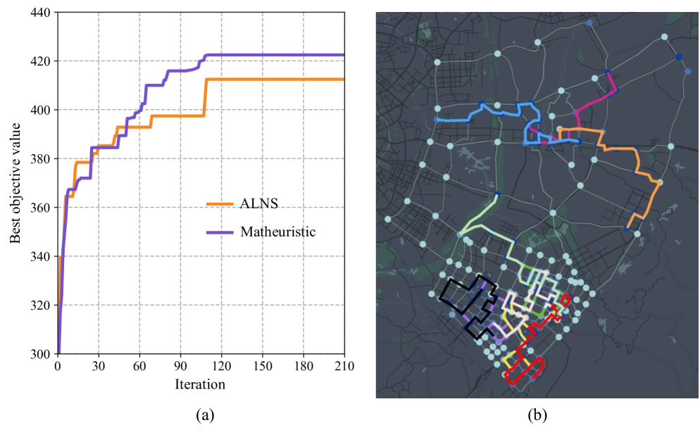
Figure 9: (a) Best objective value at each algorithm iteration; (b) visualization of the 10 routes generated by the matheuristic.

7 Conclusion

This paper proposes an extension of the team orienteering problem (TOP), named ETOP, by allowing a POI to be visited multiple times to accumulate scores. Such an extension is important because many real-world applications such as mobile sensing and disaster relief require that the POIs are continuously visited, and such needs are heterogeneous. To model such scenarios, we present the ETOP as a nonlinear integer program and propose two solution approaches: ALNS-based and matheuristic methods. The following findings are made from extensive numerical tests.

• Both algorithms are effective in finding good-quality solutions, where high-value POIs are visited more frequently. This is not achievable through solution approaches for conventional TOPs.

• On complete graphs (Figure 2), the ALNS outperforms matheuristic by a small margin, but the situation is reversed on incomplete graphs (e.g. real-world road networks), due to the limited effect of destroy and repair operators in generating new viable routes on the network.

• The ALNS is much less computationally efficient than the matheuristic, because the destroy and repair operators are typically time-consuming.

• The ETOP is transferrable to treat scenarios where the demands are concentrated on arcs instead of vertices/nodes. The resulting model can be applied to anti-dust (road sprinkler) operations or road surface condition monitoring.

8 Acknowledgement

This work is supported by the National Natural Science Foundation of China through grants 72071163 and 72101215, and the Natural Science Foundation of Sichuan Province through grants 2022NSFSC0474 and 2022NSFSC1906.

References

- Ali and Dyo, (2017) Ali, J., Dyo, V., 2017. Coverage and Mobile Sensor Placement for Vehicles on Predetermined Routes: A Greedy Heuristic Approach, in: Proceedings of the 14th International Joint Conference on e-Business and Telecommunications. Madrid, Spain, 83-88.
- (2) Chao, I., Golden, B., Wasil, E., 1996a. A fast and effective heuristic for the orienteering problem. European Journal of Operational Research, 88, 475–489.
- (3) Chao, I.-M., Golden, B. L., Wasil, E. A., 1996b. The team orienteering problem. European Journal of Operational Research, 88(3), 464–474.
- Dang et al., (2013) Dang, D.-C., Guibadj, R. N., Moukrim, A., 2013. An effective PSO-inspired algorithm for the team orienteering problem. European Journal of Operational Research, 229(2), 332–344.
- Demir et al., (2012) Demir, E., Bektaş, T., Laporte, G., 2012. An adaptive large neighborhood search heuristic for the Pollution-Routing Problem. European Journal of Operational Research, 223, 346–359.
- Duque et al., (2015) Duque, D., Lozano, L., Medaglia, A. L., 2015. Solving the orienteering problem with time windows via the pulse framework. Computers & Operations Research, 54, 168–176.
- Gambardella et al., (2012) Gambardella, L. M., Montemanni, R., Weyland, D., 2012. Coupling ant colony systems with strong local searches. European Journal of Operational Research, 220(3), 831–843.
- Golden and Wong, (1981) Golden, B. L., Wong, R. T., 1981. Capacitated routing problems. Networks, 11:305-31.
- Golden et al., (1984) Golden, B., Assad, A., Dahl, R., 1984. Analysis of a large-scale vehicle routing problem with an inventorycomponent, Large Scale Systems, 7, 181-190.
- Golden et al., (1987) Golden, B. L., Levy, L., Vohra, R., 1987. The orienteering problem. Naval Research Logistics, 34(3), 307–318.
- Gunawan et al., (2014) Gunawan, A., Yuan, Z., Lau, H. C., 2014. A mathematical model and metaheuristics for time dependent orienteering problem. In Proceedings of the 10th international conference of the practice and theory of automated timetabling (patat 2014), York, United Kingdom, 202–217.
- Gunawan et al., (2016) Gunawan, A., Lau, H.C., Vansteenwegen, P., 2016. Orienteering Problem: A survey of recent variants, solution approaches and applications. European Journal of Operational Research, 255, 315–332.
- Ilhan et al., (2008) Ilhan, T., Iravani, S. M. R., Daskin, M. S., 2008. The orienteering problem with stochastic profits. IIE Transactions, 40(4), 406–421.
- Ke et al., (2015) Ke, L., Zhai, L., Li, J., Chan, F. T. S., 2015. Pareto mimic algorithm: an approach to the team orienteering problem. Omega, 61, 155–166.
- Lin and Yu, (2012) Lin, S. W., Yu, V. F., 2012. A simulated annealing heuristic for the team orienteering problem with time windows. European Journal of Operational Research, 217(1), 94–107.
- Miller et al., (1960) Miller, C. E., Tucker, A. W., Zemlin, R. A., 1960. Integer programming formulation of traveling salesman problems. Journal of the ACM, 7(4), 326–329.
- Mishra et al., (2023) Mishra, M., Chen, P.-H., Bisquera, W., Lin, G.-Y., Le, T.-C., Dejchanchaiwong, R., Tekasakul, P., Jhang, C.-W., Wu, C.-J., Tsai, C.-J., 2023. Source-apportionment and spatial distribution analysis of VOCs and their role in ozone formation using machine learning in central-west Taiwan. Environmental Research, 232, 116329.
- Pisinger and Ropke, (2007) Pisinger, D., Ropke, S., 2007. A general heuristic for vehicle routing problems. Computers & Operations Research, 34, 2403–2435.
- Potvin and Rousseau, (1993) Potvin, J.-Y., Rousseau, J.-M., 1993. A parallel route building algorithm for the vehicle routing and scheduling problem with time windows. European Journal of Operational Research, 66, 331–340.
- Ropke and Pisinger, (2006) Ropke, S., Pisinger, D., 2006. An Adaptive Large Neighborhood Search Heuristic for the Pickup and Delivery Problem with Time Windows. Transportation Science, 40, 455–472.
- Tang et al., (2007) Tang, H., Miller-Hooks, E., Tomastik, R., 2007. Scheduling technicians for planned maintenance of geographically distributed equipment. Transportation Research Part E: Logistics and Transportation Review, 43(5), 591–609.
- Vansteenwegen and Van Oudheusden, (2007) Vansteenwegen, P., Van Oudheusden, D., 2007. The mobile tourist guide: an OR opportunity. OR Insights, 20(3), 21–27.
- Vansteenwegen et al., (2011) Vansteenwegen P., Souffriau W., Oudheusden D. V., 2011. The orienteering problem: A survey. European Journal of Operational Research, 209(1), 1–10.
- Verbeeck et al., (2014) Verbeeck, C., Sörensen, K., Aghezzaf, E. H., Vansteenwegen, P., 2014. A fast solution method for the time-dependent orienteering problem. European Journal of Operational Research, 236(2), 419–432.
- Windras Mara et al., (2022) Windras Mara, S.T., Norcahyo, R., Jodiawan, P., Lusiantoro, L., Rifai, A.P., 2022. A survey of adaptive large neighborhood search algorithms and applications. Computers & Operations Research, 146, 105903.
- Yang et al., (2020) Yang, H.-H., Gupta, S.K., Dhital, N.B., 2020. Emission factor, relative ozone formation potential and relative carcinogenic risk assessment of VOCs emitted from manufacturing industries. Sustainable Environment Research, 30, 28.
- Yu et al., (2022) Yu, Q., Adulyasak, Y., Rousseau, L.-M., Zhu, N., Ma, S., 2022. Team Orienteering with Time-Varying Profit. INFORMS Journal on Computing, 34, 262–280.
- Yu et al., (2019) Yu, Q., Fang, K., Zhu, N., Ma, S., 2019. A matheuristic approach to the orienteering problem with service time dependent profits. European Journal of Operational Research, 273, 488–503.
- Zhang et al., (2014) Zhang, S., Ohlmann, J. W., Thomas, B. W., 2014. A priori orienteering with time windows and stochastic wait times at customers. European Journal of Operational Research, 239(1), 70–79.
- Zhu et al., (2022) Zhu,B., Sun, Z., Zhou, C., Wang, X., Zhang, P., 2022. The capacitied arc routing problem for anti-dust vehicles with heterogeneous services and time-dependent profits. in: Proceedings of the Transportation Research Board of the National Academies.