CTPU-PTC-23-29

Axion-Gauge Dynamics During Inflation
as the Origin of Pulsar Timing Array Signals and Primordial Black Holes

Abstract

We demonstrate that the recently announced signal for a stochastic gravitational wave background (SGWB) from pulsar timing array (PTA) observations, if attributed to new physics, is compatible with primordial GW production due to axion-gauge dynamics during inflation. More specifically we find that axion-$U(1)$ models may lead to sufficient particle production to explain the signal while simultaneously source some fraction of sub-solar mass primordial black holes (PBHs) as a signature. Moreover there is a parity violation in GW sector, hence the model suggests chiral GW search as a concrete target for future. We further analyze the axion-$SU(2)$ coupling signatures and find that in the low/mild backreaction regime, it is incapable of producing PTA evidence and the tensor-to-scalar ratio is low at the peak, hence it overproduces scalar perturbations and PBHs.

Introduction. There is a strong evidence for a stochastic gravitational wave background (SGWB) in Pulsar Timing Array (PTA) data from the NANOGRav [1, 2], EPTA [3, 4], PPTA [5] and CPTA [6] experiments in the nHz frequency regime. While this observed signal is mainly thought to be of standard astrophysical origin sourced by supermassive black hole binary mergers [7, 8, 9], on top of astrophysical background, there may be a possibility that the data also implies SGWB of cosmological origin, such as cosmic strings [10, 11, 12, 13, 14], cosmological phase transitions [15, 16, 17, 18, 19, 20, 21, 22, 23, 24, 25, 26, 27, 28, 29, 30, 31, 32, 33], scalar induced GW (SIGW) [34, 35, 36, 37, 38, 39, 40, 41, 42, 43, 44, 45].

How about a possibility of primordial gravitational waves (GW) from cosmic inflation [46, 47, 48, 49]? In the standard inflationary model, the amplitude of SGWB is nearly scale-invariant and is parameterized by a ratio of tensor and scalar power spectra, called tensor-to-scalar ratio $r$. It is yet to be detected and current cosmic microwave background (CMB) experiments, Planck [50] and BICEP/Keck [51], have put an upper bound $r\lesssim 0.034$ at 95 % C.L. [52]. This CMB bound predicts the SGWB much smaller than that measured in PTA data. Explaining the data requires a blue-tilted spectrum around the nHz frequency regime [2, 53, 54], which is not compatible with the standard inflationary scenario producing nearly scale invariant SGWB.

In the simplest scenario discussed above, SGWB is produced by the vacuum fluctuation of the metric, and the tensor-to-scalar ratio is directly related to the energy scale of inflation. However, this is not necessarily true if additional matter fields could source the GW during inflation. In such scenarios, the dynamics of gauge fields coupled to axions, both Abelian ($U(1)$) [55, 56, 57, 58, 59, 60, 61, 62, 63, 64, 65, 66, 67, 68] and non-Abelian ($SU(2)$) [69, 70, 71, 72, 73, 74, 75, 76, 77, 78, 79, 80, 81, 82, 83] groups, have been well studied (see [84, 85] for reviews). Axions generically couple to gauge fields via topological Chern-Simons interactions, and this coupling violates the conformal invariance of the gauge field. Owing to this coupling, there is copious production of one circular polarization of the gauge field which in turn amplifies GW background during inflation. The resultant sourced SGWB is generically scale-dependent and its spectral shape is controlled by the time evolution of axion field. Therefore, depending on the potential, the sourced SGWB is enhanced on intermediate scales during inflation and is potentialy testable with future interferometers or PTAs [57, 65, 66, 67, 68, 73, 79, 86]. The amplified gauge field also inevitably sources scalar density modes, aside from GW, which could in turn lead to the generation of primordial black holes (PBHs) after inflation [66, 87, 88, 68, 89] (see also PBHs via axions [90]).

In this Letter, we show the possibility that the current PTA data can be explained by the primordial GW sourced by axion-gauge dynamics during inflation. We consider two scenarios: $U(1)$ and $SU(2)$ models. The axion is a spectator field and realizes localized gauge field amplifications on intermediate scales. We discuss the possibility of generating a enhanced power spectrum of tensor modes compatible with the NANOGrav data from these models while satisfying some theoretical consistencies. We limit our analysis to the low/mild backreaction regime for which we have robust analytic expressions and remain agnostic about the dynamics in the strong backreaction regime which require approximate numerical solutions [91, 92, 93, 94, 95, 96] or full simulations on the lattice [97, 98]. Furthermore, we discuss a possibility that the sourced power spectrum of scalar modes can lead to scalar induced GW and PBH generation [88, 99].

PTA Data. PTA experiments found evidence for the characteristic strain amplitude as [1, 2, 4])

$$h_{c}(f)=10^{-14.3\pm 0.3}\left(\frac{f}{yr^{-1}}\right)^{\gamma},$$ (1)

where $-0.5<\gamma<0.5$ in 2-$\sigma$ error bars. In terms of the GW energy density, we have

$$\Omega_{GW,0}h^{2}\simeq\left(\frac{g_{0}}{g_{*}}\right)^{1/3}\frac{2\pi^{2}}{3H_{0}^{2}}h_{c}^{2}f^{2}\ ,$$ (2)

where $g_{*,0}$ is the relativistic degrees of freedom at the time of GW formation and at present, $H_{0}$ is current Hubble parameter. Then, we evaluate $\Omega_{GW,0}\sim 10^{-7}$ implying $P_{h}\sim 10^{-2}$ around frequency $yr^{-1}$, and $\Omega_{GW,0}\sim 10^{-8}$ implying $P_{h}\sim 10^{-3}$ for $f\sim(3\,yr)^{-1}$ . This is many orders of magnitude larger than current bounds on CMB scales, ie. $P_{h,CMB}<10^{-11}$. Hence the background needs to be amplified at least 9 orders of magnitude compared to fluctuations at large scales.

Axion and U(1) Coupling. We present an inflationary model where an axion field couples to a $U(1)$ gauge field with field strength tensor $F_{\mu\nu}=\partial_{\mu}A_{\nu}-\partial_{\nu}A_{\mu}$. In this work, we consider the model where the axion coupled to the gauge field is a spectator [61, 64]. The Lagrangian density is as follows:

$$\mathcal{L} =\mathcal{L}_{\rm GR}+\mathcal{L}_{\rm inflaton}+\mathcal{L}_{\rm gauge}+\mathcal{L}_{\rm spectator}\ ,$$ (3)

$$\mathcal{L}_{\rm spectator} =-\dfrac{1}{2}\partial_{\mu}\chi\partial^{\mu}\chi-U(\chi)-\lambda\dfrac{\chi}{4f}F_{\mu\nu}\tilde{F}^{\mu\nu}\ ,$$ (4)

where $\mathcal{L}_{\rm GR}=M_{p}^{2}R/2$ and $\mathcal{L}_{\rm inflaton}=-(\partial\phi)^{2}/2-V(\phi)$ represent the Lagrangian densities of Einstein-Hilbert action and a canonical inflaton action. Regarding the inflaton potential, we let it unspecified and do not solve the background evolution of inflaton. The lagrangian density of gauge field is defined as $\mathcal{L}_{\rm gauge}=-F_{\mu\nu}F^{\mu\nu}/4$. The Hodge dual of field strength is defined as $\tilde{F}^{\mu\nu}\equiv\sqrt{-g}\epsilon^{\mu\nu\rho\sigma}F_{\rho\sigma}/2$, where $\epsilon^{\mu\nu\rho\sigma}$ is an antisymmetric tensor satisfying $\epsilon^{0123}=g^{-1}$. The important thing is that the inflaton is not directly coupled to the gauge field . This assumption enables the generation of curvature perturbations sourced by the gauge field to be suppressed.

We consider the time evolution of the gauge field coupled to a rolling axion. To do it, we decompose the gauge potential $A_{i}$ into operators with two circular polarization modes in Fourier space $\hat{A}^{\pm}_{\bm{k}}$. Then, in terms of a dimensionless time variable $x\equiv-k\tau$, the equation of motion (EoM) for the mode function $A^{\pm}_{k}$ is given by

$$\partial_{x}^{2}A^{\pm}_{k}+\left(1\mp\dfrac{2\xi}{x}\right)A^{\pm}_{k}=0\ ,\quad\xi\equiv\dfrac{\lambda\dot{\bar{\chi}}}{2fH}\ ,$$ (5)

where the dispersion relation is modified by the axion-$U(1)$ coupling controlled by a model parameter $\xi$. Initially, when the size of the mode function is deep inside the horizon ($x\gg 1$), this correction term is negligible and the gauge field obeys the standard dispersion relation. When it becomes comparable to the horizon size, however, one circular polarization mode gets an effective negative mass square for $x\lesssim 2\xi$ and a growing solution appears. The plus mode $A^{+}_{k}$ is amplified exponentially $A^{+}_{k}\propto e^{\pi\xi}$ in the time interval $(8\xi)^{-1}\lesssim x\lesssim 2\xi$. After $x\lesssim(8\xi)^{-1}$, the amplification weakens and the energy density of gauge field is diluted away by the expansion of the universe. Therefore, the gauge field production takes place at around horizon-crossing and enhances other coupled fluctuations.

This amplified gauge field enhances the coupled metric tensor modes $g_{ij}=a^{2}(\delta_{ij}+h_{ij})$ at second order level via the transverse-traceless components of energy-momentum tensor of electromagnetic field. We define the power spectrum of GW

$$\langle h_{\bm{k}}h_{\bm{k}^{\prime}}\rangle=(2\pi)^{3}\delta(\bm{k}+\bm{k}^{\prime})\dfrac{2\pi^{2}}{k^{3}}\left(P^{R}_{h}+P^{L}_{h}\right)\ ,$$ (6)

where $P^{R(L)}_{h}$ is a dimensionless right- (left-) handed tensor power spectrum. The shape of power spectrum is related to the time evolution of model parameter $\xi(t_{k})$, which is determined by the details of the axion potential. In this paper, we follow the previous works [64] and adopt a cosine potential

$$U(\chi)=\Lambda^{4}\left[\cos\left(\dfrac{\chi}{f}\right)+1\right]\ .$$ (7)

The velocity of the field gets a maximum value around $\chi(t=t_{*})=\pi f/2$. In the case of axion-$U(1)$ model, the slow-roll solution is given as

$$\xi=\dfrac{\lambda\delta}{2\cosh{[\delta H(t-t_{*})]}}\ ,\quad\delta\equiv\dfrac{\Lambda^{4}}{3H^{2}f^{2}}\ .$$ (8)

Figure 1: An example of GW production for the spectator axion-U(1) model that is in agreement with the NANOGrav signal. The chosen parameters are $\delta=0.5$, $6<\xi_{*}<6.2$, and $r_{v}=10^{-2}$ (blue). The astrophysical origin SMBHB (red), and the total SGWB (green) are also displayed.

GW Production for U(1). In Figure 1, we plot the SGWB from axion-$U(1)$ model and compare it with that from astrophysical origin [1, 2]. The astrophysical GWB from SMBHB is expected to have $10^{-15}$ characteristic strain amplitude, and -2/3 frequency slope, which translates into $\Omega_{\rm astro}\sim 10^{-9}\left(f/yr^{-1}\right)^{2/3}$. Additionally these axion-gauge field interactions produce a unique signature, namely at small frequencies it scales as $f^{3}$ consistent with the NANOGrav slope, the peak is in log-normal shape and there is a rapid decay in the UV frequencies.

Power spectra of sourced tensor and scalar mode around their peak are parametrized as [64]

$$P_{i,s}(k)=\left(\frac{H^{2}}{8\pi^{2}M_{p}^{2}}\right)^{2}f_{2,i}\qquad(i=h,\zeta)\ ,$$ (9)

where $f_{2,i}=A_{i}{\rm Exp}\left[-\ln\left(\frac{k}{x_{i}k_{*}}\right)^{2}/(2\sigma_{i}^{2})\right]$ with the amplitude $A_{i}$, the spectral width $\sigma_{i}$, and with the spectral position $x_{i}$ at which the function has the bump $k=x_{i}k_{*}$. Specifically, we have $A_{h}={\rm Exp}[-6.85+9.05\xi_{*}+0.0596\xi^{2}_{*}]$ where $\xi_{*}=\lambda\delta/2$ is the largest value of $\xi(t=t_{*})$ at the fastest motion point. We show in the shaded region the SGWB for particle production parameter in the range, $\xi_{*}=6.2$ to $\xi_{*}=6.$. We further confirm that primordial GW peak is greater than astrophysical for $\xi_{*}>5.8$. For the chosen example parameters, tensor-to-scalar ratio at the peak $r(k_{p})\sim{\rm Exp}[-0.4]\sim 1/2$. For different rolling times and particle production parameters, see [64].

A value of $P_{h}\sim 10^{-3}$ corresponds to $P_{\zeta}\sim 10^{-2.5}$ which may not violate PBH bound if fluctuations are relatively Gaussian as we will discuss in the next section. Note that although the scalar perturbations are characterized by a narrowly peaked amplitude, the GW spectrum signal is scaled as $f^{3}$ in the low frequency regime, namely in $f\ll f_{\rm peak}$. Regarding the validity of the perturbative description and effects of backreaction, we note that the values of $\xi_{*}$ explaining PTA data statistically better are close to these bounds. Beyond $\xi_{*}\gtrsim 6$ (for $\delta=0.5$), we would need a larger value of axion decay constant, closer to $M_{p}$ [101, 102]. For these parameter region, non-linear analysis becomes necessary and it is beyond the scope of our paper.

Axion and SU(2) Coupling. Next, we present an inflationary model where an axion couples to an $SU(2)$ gauge field with field strength $F^{a}_{\mu\nu}=\partial_{\mu}A_{\nu}-\partial_{\nu}A_{\mu}-g\epsilon^{abc}A^{b}_{\mu}A^{c}_{\nu}$. The original model is called chromo-natural inflation, where an inflaton is directly coupled to the $SU(2)$ field [103]. However, this model was found to be inconsistent with CMB observations [104, 105, 106]. In this paper, we adopt the spectator axion-SU(2) model [75], where the Lagrangian density is given by the same form as the $U(1)$ model (3), (4).

At the background level, the $SU(2)$ field can acquire an isotropic background value [108, 109] $\bar{A}^{a}_{i}(t)=a(t)Q(t)\delta^{a}_{i}$, which is diagonal between the indices of $SU(2)$ and $SO(3)$ algebra. Since this configuration respects the spatial isotropy, the background spacetime can be described by a simple FLRW metric. The axion-$SU(2)$ coupling in the presence of a non-zero isotropic gauge field vacuum expectation value, vev, induces a friction in the equation of motion for the axion. The vev is assumed to be at the bottom of its effective potential $Q(t)\simeq(-fU_{\chi}/(3g\lambda H))^{1/3}$ and the particle production is characterized by the parameter

$$m_{Q}=gQ/H$$ (10)

related to the $U(1)$ parameter through $\xi\simeq m_{Q}+m_{Q}^{-1}$. This solution is an attractor even if we start from the initial anisotropic parameter space as long as it leads to a stable inflationary period [110, 111, 112].

At the level of perturbations, the fluctuation of the gauge field $\delta A^{a}_{i}$ possesses the transverse-traceless mode $\delta A^{a}_{i}\supset t^{a}_{i}$ owing to the background rotational symmetry. In the presence of the background vev, the tensor modes of the gauge field couple to GW at the linear level. In an analogous manner to the $U(1)$ case only one chirality of the tensor perturbations experiences a tachyonic instability around horizon-crossing. Hence, due to the linear coupling, only one chirality mode of GW is amplified. In this paper, we assume the amplified mode is right-handed: $t_{R}$ and $h_{R}$. The ratio of the sourced fluctuations to the vacuum fluctuations takes the form [75]

$$R_{\rm GW}\equiv\frac{P_{h,s}}{P_{h,v}}=\frac{\epsilon_{B}}{2}{\cal F}^{2}$$ (11)

where $\epsilon_{B}\equiv g^{2}Q^{4}/(HM_{p})^{2}=(m_{Q}^{4}/g^{2})\;(H^{2}/M_{p}^{2})$ and $\mathcal{F}$ is a numerical factor and in the parameter range $m_{Q}\gtrsim 2$ it is approximated by $\mathcal{F}^{2}\simeq e^{3.6m_{Q}}$ [75]. Combining all, we express the primordial SGWB as follows

$$\Omega_{GW,0}h^{2}=\frac{\Omega_{\gamma,0}h^{2}}{24}\left(\frac{g_{0}}{g_{*}}\right)^{1/3}P_{h,s}$$ (12)

where $\Omega_{\gamma,0}$ is radiation energy density, and $g_{0}$ and $g_{*}$ are the relativistic degrees of freedom today and re-entry.

For the non-Abelian case in the weak backreaction regime, it can be shown that the sourced GW can not be compatible with the NANOGrav signal. The main challenge of achieving the desired signal is due to the severe restriction imposed by the backreaction constraint. Unlike the axion-$U(1)$ case, the backreaction generally affects the EoM of the gauge field vev first (which is not present in the axion-$U(1)$ case) before there is a chance to backreact in the EoM of the axion, hence there are tighter constraints on the particle production parameter $m_{Q}$ compared to the Abelian equivalent $\xi$ [113, 101]. We extend the analysis given in detail in section 5.2 of [114]. We present our combined constraints in Figure 2 which is valid for small scales and contains the SGWB amplitude. By requiring that the sourced GW is of the order of the NANOGrav signal (e.g. $\Omega_{\rm GW}h^{2}\sim 10^{-8}$), we can produce an additional line on the same figure that transparently displays what it would take to account for the NANOGrav signal.

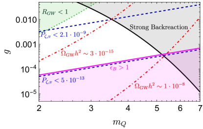
Figure 2: Constraints for the case of the axion-SU(2) model. The black contour displays the regime for which the backreaction is relevant (13) and therefore beyond the scope of this work. The two blue dashed lines indicate the corresponding value of the vacuum contribution to the power spectrum of scalar perturbations (15). The two red lines display the level of sourced GW production assuming $P_{h,v}$ the maximum allowed from CMB observations. Finally the magenta contour is disallowed because it would require for the slow-roll parameter to be greater than unity.

We impose the same backreaction constraint

$$g\ll\left(\frac{24\pi^{2}}{2.3\cdot{\rm e}^{3.9m_{Q}}}\frac{1}{1+\frac{1}{m_{Q}^{2}}}\right)^{1/2}$$ (13)

which arises by demanding that the backreaction term in the EoM of the vev is smaller than the smallest background term, as in Ref. [114]. This is the safer condition due to a cancellation among the various terms as outlined in [113] (see also [115, 116] for the Schwinger effect).

We could relax the normalization of $P_{\zeta,v}$ at small scales which is not constrained. The vacuum contribution to the power spectrum takes the form [114]

$$P_{\zeta,v}\simeq\frac{H^{2}}{8\pi^{2}M_{p}^{2}}\frac{\epsilon_{\phi}}{\sum_{i}\epsilon_{i}^{2}}=\frac{g^{2}}{8\pi^{2}m_{Q}^{4}}\frac{\epsilon_{\phi}\epsilon_{B}}{\left(\epsilon_{\phi}+\epsilon_{B}\right)^{2}}$$ (14)

which further implies an absolute maximum value or $P_{\zeta,v}$ for a given $g$ and $m_{Q}$, namely

$$P_{\zeta,v,{\rm max}}\simeq\frac{g^{2}}{32\pi^{2}m_{Q}^{4}}$$ (15)

We plot the maximum attainable value of $P_{\zeta,v}$ for particular choices of $m_{Q}$ and g on Figure 2 for reference. Naively one might think that values of $P_{\zeta,v}$ much lower than the CMB normalization are difficult to achieve, however that is not as clear cut in the non-Abelian model since there are several branches of solutions depending on the hierarchy of the slow roll parameters (for more details see Appendix F of [114]). In that case there is a lot more freedom to choose the various parameters, however for small $g$ and large $m_{Q}$ one inevitably enters the regime for which the slow-roll parameter $\epsilon_{B}$ is greater than one. Such a value is unacceptable as it would be incompatible with inflation. We plot some sample values of $P_{\zeta,v}$ in Figure 2 and superimpose the corresponding sourced GW power spectrum for some sample choices. The upper red line is the maximum produced sourced GW allowed if we assume a flat spectrum for $P_{\zeta,v}$ from CMB to PTA scales and the lower red line is the parameter space that would account for the NANOGrav signal while being agnostic about the evolution of $P_{\zeta,v}$ at small scales. Note that we assumed for $P_{h,v}$ the maximum allowed value by CMB observations and a flat spectrum. This yields the absolute best case scenario and relaxing it makes the incompatibility even worse.

Finally, we would like to point out that one can obtain an even more severe restriction in the parameter space displayed in Figure 2 by investigating whether for the NANOGrav signal at the peak $r_{\rm tot}\sim 1$ holds, which is a necessary condition for the non-overproduction of PBH. Specifically, using formulas (5.1) and (5.9) of [114] in which the sourced contributions dominate over the vacuum at the peak of the signal in the $\epsilon_{B}>\epsilon_{\phi}$ branch (Appendix F of the same reference), we have

$$r(k_{p})\simeq\frac{8.5\cdot 10^{-2}}{N_{k}^{2}}\frac{\epsilon_{B}}{\epsilon_{\phi}}\;\left(\frac{m_{Q}}{3.4}\right)^{-11}\;e^{-3.4(m_{Q}-3.4)}\;.$$ (16)

This ratio is always much smaller than one for $m_{Q}>3.4$ which implies that the large values of $m_{Q}$ required to explain the NANOGrav signal are certain to overproduce scalar density perturbations, and expectedly PBH.

In summary, our analysis indicates that the NANOGrav signal observed is highly unlikely to be due to axion-$SU(2)$ dynamics during inflation in the low backreaction regime. It would be interesting to expand our analysis to the strong backreaction regime as in [117]. However, such numerical analysis is beyond the scope of the current work.

PBH formation and Induced GW. PBHs are produced in large abundances with higher efficiency, especially in the case of large non-Gaussianity. For same PBH abundance, the following relation holds between Gaussian and chi-square ($\chi^{2}$) non-Gaussian density perturbations [88, 87]

$$P_{\zeta,{\chi^{2}}}\sim\frac{2}{\zeta_{c}^{2}}\;P_{\zeta,G}^{2}\ .$$ (17)

$\zeta_{c}\sim\frac{3}{2}\delta_{c}$ is the critical threshold for curvature perturbations. Hence, for considerable PBH abundances we have $P_{\zeta,G}\sim 2\cdot 10^{-2}$, and $P_{\zeta,\chi^{2}}\sim 10^{-3}$. For given amplitude and peak frequency, we estimate a PBH population, ranging from $10^{-10:-2}$ fraction of dark matter concentrated in masses about $10^{-4}-10^{-1}M_{\odot}$ .

It has been shown that as the fluctuations grow, they are highly non-Gaussian and approach the $\chi^{2}$ distribution. However, simulations [97] conducted in the case of the axion-$U(1)$ model reveals that near the peak scalar perturbation statistics deviate from a $\chi^{2}$ distribution and converge to a Gaussian due to non-coherent addition of modes, thus weakening the PBH bound, allowing to some extent higher amplitude perturbations (See also recent results [98] discovering the UV regime of momentum distribution.). We expect the same trend to exist in the case of axion-$SU(2)$.

Enhanced scalar perturbations also source GW, scalar induced GW. In axion inflation models, the primordial GW spectrum is larger than scalar induced GW background, which is also the case in our result, for given parameters $\Omega_{{\rm SIGW,\,peak}}\sim 10^{-9}$, and leave the spectrum details to future work.

Discussion and Conclusions. The newly released PTA measurements show evidence for a SGWB. Although compatible with a background arising from supermassive black bole binary mergers, it is interesting to interpret the signal as having an early universe origin.

We show that it is possible with axion-gauge field interactions during inflation. There are two main contributions to SGWB, one from sourced primordial GW background and the other from scalar induced GW (SIGW) background resulting from enhanced scalar perturbations. However, explaining the PTA signal with SIGW is a hard task due to PBH overproduction. Remarkably, in axion inflation, primordial GW production usually dominates over SIGW, namely primordial production is more dominant compared to SIGW, hence it allows a chance to explain the PTA data, and at the same time generating interesting signatures such sub-dominant fraction dark matter in primordial black holes and another SGWB, called scalar induced GW background.

We employ two models to explain the signal via this mechanism. The first one is an axion coupled to an Abelian gauge field [64, 66]. The axion rolls down for a finite period during inflation and when its speed is maximum, it sources one chirality of the gauge field. As a result the amplified gauge field sources one chirality of GW, axion and inflaton perturbations. The low frequency regime of the GW signal scales with $f^{3}$ instead of a log-normal fall, which improves the fit considerably together with the astrophysical background.

The second model is an axion coupled to a non-Abelian gauge field in which due to the non-zero, isotropic, vacuum expectation value of the gauge field, there is a linear coupling between GW and the gauge field [106, 75], and the scalar modes are sourced via a cubic coupling [118, 114]. The model requires large amplification of gauge modes such that GW can explain the PTA data, but this amplification results in two potential pitfalls i) strong backreaction and ii) low tensor-to-scalar ratio at the peak, both of which are very difficult to overcome.

We show that the axion-$U(1)$ model, for a finite amount of rolling, potentially explains the deviation from astrophysical background in PTA data, and is consistent with the given spectral shape, together with interesting phenomenological signatures such as chiral primordial GW, scalar induced GW and PBH production. We find that such a parameter region is not excluded but is close to the perturbativity and backreaction bounds derived in small/mild backreaction regime, and thereby there is a need for non-linear analysis. We also note that there is a clear smoking gun of axion inflation coupled to gauge fields, namely statistical parity violation, hence it is expected that the resultant GW background is almost perfectly chiral , which is a concrete prediction for forthcoming surveys [120, 121, 122, 123, 124].

Acknowledgement. We are grateful to Robert Caldwell, Angelo Caravano, Emanuela Dimastrogiovanni, Matteo Fasiello, Daniel G. Figueroa and Eiichiro Komatsu for the comments on the draft. C.U. thanks Yann Gouttenoire and Lorenzo Sorbo for the discussions on effective degrees of freedom from gauge fields. C.U. dedicates this work to Harun Kolçak, and thanks his family for their support. C.U. is supported by the Kreitman fellowship of the Ben-Gurion University, and the Excellence fellowship of the Israel Academy of Sciences and Humanities, and the Council for Higher Education, and dedicates this work to Harun Kolçak. A.P. is supported by IBS under the project code, IBS-R018-D1. I.O. is supported by JSPS KAKENHI Grant No. JP20H05859 and 19K14702.

References

- Agazie et al. [2023] G. Agazie et al. (NANOGrav), Astrophys. J. Lett. 951 (2023), 10.3847/2041-8213/acdac6, arXiv:2306.16213 [astro-ph.HE] .
- Afzal et al. [2023] A. Afzal et al. (NANOGrav), Astrophys. J. Lett. 951 (2023), 10.3847/2041-8213/acdc91, arXiv:2306.16219 [astro-ph.HE] .
- Antoniadis et al. [2023a] J. Antoniadis et al., (2023a), arXiv:2306.16214 [astro-ph.HE] .
- Antoniadis et al. [2023b] J. Antoniadis et al., (2023b), arXiv:2306.16227 [astro-ph.CO] .
- Reardon et al. [2023] D. J. Reardon et al., Astrophys. J. Lett. 951 (2023), 10.3847/2041-8213/acdd02, arXiv:2306.16215 [astro-ph.HE] .
- Xu et al. [2023] H. Xu et al., (2023), 10.1088/1674-4527/acdfa5, arXiv:2306.16216 [astro-ph.HE] .
- Pol et al. [2021] N. S. Pol et al. (NANOGrav), Astrophys. J. Lett. 911, L34 (2021), arXiv:2010.11950 [astro-ph.HE] .
- Middleton et al. [2021] H. Middleton, A. Sesana, S. Chen, A. Vecchio, W. Del Pozzo, and P. A. Rosado, Mon. Not. Roy. Astron. Soc. 502, L99 (2021), arXiv:2011.01246 [astro-ph.HE] .
- Broadhurst et al. [2023] T. Broadhurst, C. Chen, T. Liu, and K.-F. Zheng, (2023), arXiv:2306.17821 [astro-ph.HE] .
- Ellis and Lewicki [2021] J. Ellis and M. Lewicki, Phys. Rev. Lett. 126, 041304 (2021), arXiv:2009.06555 [astro-ph.CO] .
- Blasi et al. [2021] S. Blasi, V. Brdar, and K. Schmitz, Phys. Rev. Lett. 126, 041305 (2021), arXiv:2009.06607 [astro-ph.CO] .
- Samanta and Datta [2021] R. Samanta and S. Datta, JHEP 05, 211 (2021), arXiv:2009.13452 [hep-ph] .
- Ellis et al. [2023] J. Ellis, M. Lewicki, C. Lin, and V. Vaskonen, (2023), arXiv:2306.17147 [astro-ph.CO] .
- Wang et al. [2023a] Z. Wang, L. Lei, H. Jiao, L. Feng, and Y.-Z. Fan, (2023a), arXiv:2306.17150 [astro-ph.HE] .
- Higaki et al. [2016] T. Higaki, K. S. Jeong, N. Kitajima, T. Sekiguchi, and F. Takahashi, JHEP 08, 044 (2016), arXiv:1606.05552 [hep-ph] .
- Kobakhidze et al. [2017] A. Kobakhidze, C. Lagger, A. Manning, and J. Yue, Eur. Phys. J. C 77, 570 (2017), arXiv:1703.06552 [hep-ph] .
- Arunasalam et al. [2018] S. Arunasalam, A. Kobakhidze, C. Lagger, S. Liang, and A. Zhou, Phys. Lett. B 776, 48 (2018), arXiv:1709.10322 [hep-ph] .
- Nakai et al. [2021] Y. Nakai, M. Suzuki, F. Takahashi, and M. Yamada, Phys. Lett. B 816, 136238 (2021), arXiv:2009.09754 [astro-ph.CO] .
- Ratzinger and Schwaller [2021] W. Ratzinger and P. Schwaller, SciPost Phys. 10, 047 (2021), arXiv:2009.11875 [astro-ph.CO] .
- Neronov et al. [2021] A. Neronov, A. Roper Pol, C. Caprini, and D. Semikoz, Phys. Rev. D 103, 041302 (2021), arXiv:2009.14174 [astro-ph.CO] .
- Chiang and Lu [2021] C.-W. Chiang and B.-Q. Lu, JCAP 05, 049 (2021), arXiv:2012.14071 [hep-ph] .
- Arzoumanian et al. [2021] Z. Arzoumanian et al. (NANOGrav), Phys. Rev. Lett. 127, 251302 (2021), arXiv:2104.13930 [astro-ph.CO] .
- Ferreira et al. [2023] R. Z. Ferreira, A. Notari, O. Pujolas, and F. Rompineve, JCAP 02, 001 (2023), arXiv:2204.04228 [astro-ph.CO] .
- Ashoorioon et al. [2022] A. Ashoorioon, K. Rezazadeh, and A. Rostami, Phys. Lett. B 835, 137542 (2022), arXiv:2202.01131 [astro-ph.CO] .
- Han et al. [2023] C. Han, K.-P. Xie, J. M. Yang, and M. Zhang, (2023), arXiv:2306.16966 [hep-ph] .
- Li et al. [2023] Y. Li, C. Zhang, Z. Wang, M. Cui, Y.-L. S. Tsai, Q. Yuan, and Y.-Z. Fan, (2023), arXiv:2306.17124 [astro-ph.HE] .
- Fujikura et al. [2023] K. Fujikura, S. Girmohanta, Y. Nakai, and M. Suzuki, (2023), arXiv:2306.17086 [hep-ph] .
- Kitajima et al. [2023] N. Kitajima, J. Lee, K. Murai, F. Takahashi, and W. Yin, (2023), arXiv:2306.17146 [hep-ph] .
- Athron et al. [2023] P. Athron, A. Fowlie, C.-T. Lu, L. Morris, L. Wu, Y. Wu, and Z. Xu, (2023), arXiv:2306.17239 [hep-ph] .
- Blasi et al. [2023] S. Blasi, A. Mariotti, A. Rase, and A. Sevrin, (2023), arXiv:2306.17830 [hep-ph] .
- Lu and Chiang [2023] B.-Q. Lu and C.-W. Chiang, (2023), arXiv:2307.00746 [hep-ph] .
- Li and Xie [2023] S.-P. Li and K.-P. Xie, (2023), arXiv:2307.01086 [hep-ph] .
- Ghosh et al. [2023] T. Ghosh, A. Ghoshal, H.-K. Guo, F. Hajkarim, S. F. King, K. Sinha, X. Wang, and G. White, (2023), arXiv:2307.02259 [astro-ph.HE] .
- Chen et al. [2020] Z.-C. Chen, C. Yuan, and Q.-G. Huang, Phys. Rev. Lett. 124, 251101 (2020), arXiv:1910.12239 [astro-ph.CO] .
- Wang et al. [2019] S. Wang, T. Terada, and K. Kohri, Phys. Rev. D 99, 103531 (2019), [Erratum: Phys.Rev.D 101, 069901 (2020)], arXiv:1903.05924 [astro-ph.CO] .
- Vaskonen and Veermäe [2021] V. Vaskonen and H. Veermäe, Phys. Rev. Lett. 126, 051303 (2021), arXiv:2009.07832 [astro-ph.CO] .
- De Luca et al. [2021] V. De Luca, G. Franciolini, and A. Riotto, Phys. Rev. Lett. 126, 041303 (2021), arXiv:2009.08268 [astro-ph.CO] .
- Kohri and Terada [2021] K. Kohri and T. Terada, Phys. Lett. B 813, 136040 (2021), arXiv:2009.11853 [astro-ph.CO] .
- Domènech and Pi [2022] G. Domènech and S. Pi, Sci. China Phys. Mech. Astron. 65, 230411 (2022), arXiv:2010.03976 [astro-ph.CO] .
- Zhao and Wang [2023] Z.-C. Zhao and S. Wang, Universe 9, 157 (2023), arXiv:2211.09450 [astro-ph.CO] .
- Franciolini et al. [2023] G. Franciolini, A. Iovino, Junior., V. Vaskonen, and H. Veermae, (2023), arXiv:2306.17149 [astro-ph.CO] .
- Inomata et al. [2023] K. Inomata, K. Kohri, and T. Terada, (2023), arXiv:2306.17834 [astro-ph.CO] .
- Liu et al. [2023] L. Liu, Z.-C. Chen, and Q.-G. Huang, (2023), arXiv:2307.01102 [astro-ph.CO] .
- Wang et al. [2023b] S. Wang, Z.-C. Zhao, J.-P. Li, and Q.-H. Zhu, (2023b), arXiv:2307.00572 [astro-ph.CO] .
- Cai et al. [2023] Y.-F. Cai, X.-C. He, X. Ma, S.-F. Yan, and G.-W. Yuan, (2023), arXiv:2306.17822 [gr-qc] .
- Guth [1981] A. H. Guth, Phys. Rev. D23, 347 (1981).
- Sato [1981] K. Sato, Mon. Not. Roy. Astron. Soc. 195, 467 (1981).
- Linde [1982] A. D. Linde, Second Seminar on Quantum Gravity Moscow, USSR, October 13-15, 1981, Phys. Lett. 108B, 389 (1982).
- Albrecht and Steinhardt [1982] A. Albrecht and P. J. Steinhardt, Phys. Rev. Lett. 48, 1220 (1982).
- Tristram et al. [2021a] M. Tristram et al., Astron. Astrophys. 647, A128 (2021a), arXiv:2010.01139 [astro-ph.CO] .
- Ade et al. [2018] P. A. R. Ade et al. (BICEP2, Keck Array), Phys. Rev. Lett. 121, 221301 (2018), arXiv:1810.05216 [astro-ph.CO] .
- Tristram et al. [2021b] M. Tristram et al., (2021b), arXiv:2112.07961 [astro-ph.CO] .
- Vagnozzi [2023] S. Vagnozzi, (2023), arXiv:2306.16912 [astro-ph.CO] .
- Datta [2023] S. Datta, (2023), arXiv:2307.00646 [hep-ph] .
- Sorbo [2011] L. Sorbo, JCAP 1106, 003 (2011), arXiv:1101.1525 [astro-ph.CO] .
- Barnaby et al. [2011] N. Barnaby, R. Namba, and M. Peloso, JCAP 04, 009 (2011), arXiv:1102.4333 [astro-ph.CO] .
- Cook and Sorbo [2012] J. L. Cook and L. Sorbo, Phys. Rev. D85, 023534 (2012), [Erratum: Phys. Rev.D86,069901(2012)], arXiv:1109.0022 [astro-ph.CO] .
- Barnaby et al. [2012a] N. Barnaby, E. Pajer, and M. Peloso, Phys. Rev. D 85, 023525 (2012a), arXiv:1110.3327 [astro-ph.CO] .
- Barnaby et al. [2012b] N. Barnaby, J. Moxon, R. Namba, M. Peloso, G. Shiu, and P. Zhou, Phys. Rev. D86, 103508 (2012b), arXiv:1206.6117 [astro-ph.CO] .
- Cook and Sorbo [2013] J. L. Cook and L. Sorbo, JCAP 1311, 047 (2013), arXiv:1307.7077 [astro-ph.CO] .
- Mukohyama et al. [2014] S. Mukohyama, R. Namba, M. Peloso, and G. Shiu, JCAP 08, 036 (2014), arXiv:1405.0346 [astro-ph.CO] .
- Ferreira and Sloth [2014] R. Z. Ferreira and M. S. Sloth, JHEP 12, 139 (2014), arXiv:1409.5799 [hep-ph] .
- Peloso and Unal [2015] M. Peloso and C. Unal, JCAP 06, 040 (2015), arXiv:1504.02784 [astro-ph.CO] .
- Namba et al. [2016] R. Namba, M. Peloso, M. Shiraishi, L. Sorbo, and C. Unal, JCAP 1601, 041 (2016), arXiv:1509.07521 [astro-ph.CO] .
- Domcke et al. [2016] V. Domcke, M. Pieroni, and P. Binétruy, JCAP 06, 031 (2016), arXiv:1603.01287 [astro-ph.CO] .
- Garcia-Bellido et al. [2016] J. Garcia-Bellido, M. Peloso, and C. Unal, JCAP 12, 031 (2016), arXiv:1610.03763 [astro-ph.CO] .
- Obata [2017] I. Obata, JCAP 06, 050 (2017), arXiv:1612.08817 [astro-ph.CO] .
- Özsoy [2021] O. Özsoy, JCAP 04, 040 (2021), arXiv:2005.10280 [astro-ph.CO] .
- Maleknejad and Sheikh-Jabbari [2013a] A. Maleknejad and M. M. Sheikh-Jabbari, Phys. Lett. B 723, 224 (2013a), arXiv:1102.1513 [hep-ph] .
- Dimastrogiovanni and Peloso [2013a] E. Dimastrogiovanni and M. Peloso, Phys. Rev. D 87, 103501 (2013a), arXiv:1212.5184 [astro-ph.CO] .
- Adshead et al. [2013a] P. Adshead, E. Martinec, and M. Wyman, JHEP 09, 087 (2013a), arXiv:1305.2930 [hep-th] .
- Adshead et al. [2013b] P. Adshead, E. Martinec, and M. Wyman, Phys. Rev. D 88, 021302 (2013b), arXiv:1301.2598 [hep-th] .
- Obata and Soda [2016a] I. Obata and J. Soda, Phys. Rev. D93, 123502 (2016a), arXiv:1602.06024 [hep-th] .
- Obata and Soda [2016b] I. Obata and J. Soda, Phys. Rev. D 94, 044062 (2016b), arXiv:1607.01847 [astro-ph.CO] .
- Dimastrogiovanni et al. [2017] E. Dimastrogiovanni, M. Fasiello, and T. Fujita, JCAP 01, 019 (2017), arXiv:1608.04216 [astro-ph.CO] .
- Adshead et al. [2016] P. Adshead, E. Martinec, E. I. Sfakianakis, and M. Wyman, JHEP 12, 137 (2016), arXiv:1609.04025 [hep-th] .
- Agrawal et al. [2018a] A. Agrawal, T. Fujita, and E. Komatsu, Phys. Rev. D97, 103526 (2018a), arXiv:1707.03023 [astro-ph.CO] .
- Adshead and Sfakianakis [2017] P. Adshead and E. I. Sfakianakis, JHEP 08, 130 (2017), arXiv:1705.03024 [hep-th] .
- Thorne et al. [2018] B. Thorne, T. Fujita, M. Hazumi, N. Katayama, E. Komatsu, and M. Shiraishi, Phys. Rev. D 97, 043506 (2018), arXiv:1707.03240 [astro-ph.CO] .
- Agrawal et al. [2018b] A. Agrawal, T. Fujita, and E. Komatsu, JCAP 1806, 027 (2018b), arXiv:1802.09284 [astro-ph.CO] .
- Domcke et al. [2019] V. Domcke, B. Mares, F. Muia, and M. Pieroni, JCAP 04, 034 (2019), arXiv:1807.03358 [hep-ph] .
- Fujita et al. [2019] T. Fujita, E. I. Sfakianakis, and M. Shiraishi, JCAP 05, 057 (2019), arXiv:1812.03667 [astro-ph.CO] .
- Fujita et al. [2022] T. Fujita, K. Murai, I. Obata, and M. Shiraishi, JCAP 01, 007 (2022), arXiv:2109.06457 [astro-ph.CO] .
- Maleknejad et al. [2013] A. Maleknejad, M. M. Sheikh-Jabbari, and J. Soda, Phys. Rept. 528, 161 (2013), arXiv:1212.2921 [hep-th] .
- Komatsu [2022] E. Komatsu, Nature Rev. Phys. 4, 452 (2022), arXiv:2202.13919 [astro-ph.CO] .
- Campeti et al. [2021] P. Campeti, E. Komatsu, D. Poletti, and C. Baccigalupi, JCAP 01, 012 (2021), arXiv:2007.04241 [astro-ph.CO] .
- Domcke et al. [2017] V. Domcke, F. Muia, M. Pieroni, and L. T. Witkowski, JCAP 07, 048 (2017), arXiv:1704.03464 [astro-ph.CO] .
- Garcia-Bellido et al. [2017] J. Garcia-Bellido, M. Peloso, and C. Unal, JCAP 09, 013 (2017), arXiv:1707.02441 [astro-ph.CO] .
- Özsoy and Lalak [2021] O. Özsoy and Z. Lalak, JCAP 01, 040 (2021), arXiv:2008.07549 [astro-ph.CO] .
- Guo et al. [2023] S.-Y. Guo, M. Khlopov, X. Liu, L. Wu, Y. Wu, and B. Zhu, (2023), arXiv:2306.17022 [hep-ph] .
- Cheng et al. [2016] S.-L. Cheng, W. Lee, and K.-W. Ng, Phys. Rev. D 93, 063510 (2016), arXiv:1508.00251 [astro-ph.CO] .
- Notari and Tywoniuk [2016] A. Notari and K. Tywoniuk, JCAP 12, 038 (2016), arXiv:1608.06223 [hep-th] .
- Sobol et al. [2019] O. O. Sobol, E. V. Gorbar, and S. I. Vilchinskii, Phys. Rev. D 100, 063523 (2019), arXiv:1907.10443 [astro-ph.CO] .
- Dall’Agata et al. [2020] G. Dall’Agata, S. González-Martín, A. Papageorgiou, and M. Peloso, JCAP 08, 032 (2020), arXiv:1912.09950 [hep-th] .
- Domcke et al. [2020] V. Domcke, V. Guidetti, Y. Welling, and A. Westphal, JCAP 09, 009 (2020), arXiv:2002.02952 [astro-ph.CO] .
- Gorbar et al. [2021] E. V. Gorbar, K. Schmitz, O. O. Sobol, and S. I. Vilchinskii, Phys. Rev. D 104, 123504 (2021), arXiv:2109.01651 [hep-ph] .
- Caravano et al. [2022] A. Caravano, E. Komatsu, K. D. Lozanov, and J. Weller, (2022), arXiv:2204.12874 [astro-ph.CO] .
- Figueroa et al. [2023] D. G. Figueroa, J. Lizarraga, A. Urio, and J. Urrestilla, (2023), arXiv:2303.17436 [astro-ph.CO] .
- Ünal et al. [2021] C. Ünal, E. D. Kovetz, and S. P. Patil, Phys. Rev. D 103, 063519 (2021), arXiv:2008.11184 [astro-ph.CO] .
- Niu and Rahat [2023] X. Niu and M. H. Rahat, (2023), arXiv:2307.01192 [hep-ph] .
- Peloso et al. [2016] M. Peloso, L. Sorbo, and C. Unal, JCAP 09, 001 (2016), arXiv:1606.00459 [astro-ph.CO] .
- Campeti et al. [2022] P. Campeti, O. Özsoy, I. Obata, and M. Shiraishi, JCAP 07, 039 (2022), arXiv:2203.03401 [astro-ph.CO] .
- Adshead and Wyman [2012] P. Adshead and M. Wyman, Phys. Rev. Lett. 108, 261302 (2012), arXiv:1202.2366 [hep-th] .
- Dimastrogiovanni and Peloso [2013b] E. Dimastrogiovanni and M. Peloso, Phys. Rev. D87, 103501 (2013b), arXiv:1212.5184 [astro-ph.CO] .
- Adshead et al. [2013c] P. Adshead, E. Martinec, and M. Wyman, Phys. Rev. D88, 021302 (2013c), arXiv:1301.2598 [hep-th] .
- Adshead et al. [2013d] P. Adshead, E. Martinec, and M. Wyman, JHEP 09, 087 (2013d), arXiv:1305.2930 [hep-th] .
- Bagherian et al. [2023] H. Bagherian, M. Reece, and W. L. Xu, JHEP 01, 099 (2023), arXiv:2207.11262 [hep-th] .
- Maleknejad and Sheikh-Jabbari [2011] A. Maleknejad and M. Sheikh-Jabbari, Phys. Rev. D 84, 043515 (2011), arXiv:1102.1932 [hep-ph] .
- Maleknejad and Sheikh-Jabbari [2013b] A. Maleknejad and M. M. Sheikh-Jabbari, Phys. Lett. B723, 224 (2013b), arXiv:1102.1513 [hep-ph] .
- Maleknejad and Erfani [2014] A. Maleknejad and E. Erfani, JCAP 03, 016 (2014), arXiv:1311.3361 [hep-th] .
- Wolfson et al. [2020] I. Wolfson, A. Maleknejad, and E. Komatsu, (2020), arXiv:2003.01617 [gr-qc] .
- Wolfson et al. [2021] I. Wolfson, A. Maleknejad, T. Murata, E. Komatsu, and T. Kobayashi, JCAP 09, 031 (2021), arXiv:2105.06259 [gr-qc] .
- Maleknejad and Komatsu [2019] A. Maleknejad and E. Komatsu, JHEP 05, 174 (2019), arXiv:1808.09076 [hep-ph] .
- Papageorgiou et al. [2019] A. Papageorgiou, M. Peloso, and C. Unal, JCAP 07, 004 (2019), arXiv:1904.01488 [astro-ph.CO] .
- Lozanov et al. [2019] K. D. Lozanov, A. Maleknejad, and E. Komatsu, JHEP 02, 041 (2019), arXiv:1805.09318 [hep-th] .
- Mirzagholi et al. [2020] L. Mirzagholi, A. Maleknejad, and K. D. Lozanov, Phys. Rev. D 101, 083528 (2020), arXiv:1905.09258 [hep-th] .
- Ishiwata et al. [2022] K. Ishiwata, E. Komatsu, and I. Obata, JCAP 03, 010 (2022), arXiv:2111.14429 [hep-ph] .
- Papageorgiou et al. [2018] A. Papageorgiou, M. Peloso, and C. Unal, JCAP 09, 030 (2018), arXiv:1806.08313 [astro-ph.CO] .
- Garcia-Bellido et al. [2023] J. Garcia-Bellido, A. Papageorgiou, M. Peloso, and L. Sorbo, (2023), arXiv:2303.13425 [astro-ph.CO] .
- Crowder et al. [2013] S. G. Crowder, R. Namba, V. Mandic, S. Mukohyama, and M. Peloso, Phys. Lett. B 726, 66 (2013), arXiv:1212.4165 [astro-ph.CO] .
- Kato and Soda [2016] R. Kato and J. Soda, Phys. Rev. D 93, 062003 (2016), arXiv:1512.09139 [gr-qc] .
- Smith and Caldwell [2017] T. L. Smith and R. Caldwell, Phys. Rev. D 95, 044036 (2017), arXiv:1609.05901 [gr-qc] .
- Belgacem and Kamionkowski [2020] E. Belgacem and M. Kamionkowski, Phys. Rev. D 102, 023004 (2020), arXiv:2004.05480 [astro-ph.CO] .
- Sato-Polito and Kamionkowski [2022] G. Sato-Polito and M. Kamionkowski, Phys. Rev. D 106, 023004 (2022), arXiv:2111.05867 [astro-ph.CO] .