Molecular Abundance of the Circumnuclear Region Surrounding an Active Galactic Nucleus
in NGC 1068 based on Imaging Line Survey in the 3-mm Band with ALMA

Abstract

We present an imaging molecular line survey in the 3-mm band (85–114 GHz) focused on one of the nearest galaxies with an active galactic nucleus (AGN), NGC 1068, based on observations taken with the Atacama Large Millimeter/submillimeter Array (ALMA). Distributions of 23 molecular transitions are obtained in the central $\sim$3 kpc region, including both the circumnuclear disk (CND) and starburst ring (SBR) with 60 and 350 pc resolution. The column densities and relative abundances of all the detected molecules are estimated under the assumption of local thermodynamic equilibrium in the CND and SBR. Then, we discuss the physical and chemical effects of the AGN on molecular abundance corresponding to the observation scale. We found that H¹³CN, SiO, HCN, and H¹³CO⁺ are abundant in the CND relative to the SBR. In contrast, ¹³CO is more abundant in the SBR. Based on the calculated column density ratios of $N$(HCN)/$N$(HCO⁺), $N$(HCN)/$N$(CN), and other molecular distributions, we conclude that the enhancement of HCN in the CND may be due to high-temperature environments resulting from strong shocks, which are traced by the SiO emission. Moreover, the abundance of CN in the CND is significantly lower than the expected value of the model calculations in the region affected by strong radiation. The expected strong X-ray irradiation from the AGN has a relatively lower impact on the molecular abundance in the CND than mechanical feedback.

1 Introduction

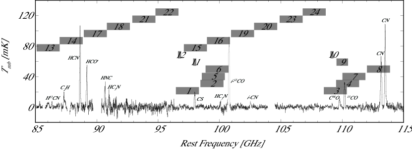
Figure 1: The gray rectangles represent the frequency coverage of each spectral window, and the numbers correspond to the setup number in Table 2. The background spectrum was obtained in NGC 1068 with the Nobeyama 45-m telescope in a previous observation (Takano et al., 2019).

To better understand the galactic power sources associated with galaxy evolution, it is important to investigate the physical/chemical properties of a nucleus in galaxies using molecular lines, which are likely to be interstellar gas tracers free from dust extinction. Several extreme and large-scale phenomena, such as starbursts, active galactic nuclei (AGNs), and merging occur in external galaxies, unlike local objects in the Milky Way. Thus far, systematic unbiased spectral scans (i.e., molecular line surveys) have been performed for typical nuclear starbursts, AGNs, and (ultra-)luminous infrared galaxies [(U)LIRGs] using large single-dish telescopes. For example, there have been reports that focus on NGC 253, NGC 1068, NGC 7469, Arp 220, Arp 157, Mrk 231, M51, M82, M83, and NGC 3627 using the IRAM 30-m telescope (Martín et al., 2006; Davis et al., 2013; Aladro et al., 2015; Watanabe et al., 2019; Qiu et al., 2020), and that focus on NGC 253, NGC 1068, IC 342, IC 10, and NGC 3627 with the NRO 45-m telescope (Nishimura et al., 2016; Nakajima et al., 2018; Takano et al., 2019; Watanabe et al., 2019). Details of previous line surveys of galaxies are listed in Martín et al. (2021). Recently, an important and interesting issue about galaxies has been the investigation of power sources in active galaxies, focusing especially on the obscured galactic nuclei, which are the central engines of the galaxy starburst or AGN. Observations revealing the power sources may provide key information regarding the evolution of galaxies.

The chemistry-based approach, which involves the use of line surveys in galaxies, is an effective way of solving this problem. From this perspective, some observations and comparative considerations of the central regions of nearby starburst galaxies and AGNs have been carried out using single-dish telescopes. Aladro et al. (2015) and Takano et al. (2019) observed the starburst galaxies and AGNs in the 3-mm band using the IRAM 30-m telescope and the NRO 45-m telescope, respectively. These studies reported that some molecules are best suited to characterize the chemistry of each type of power source. For example, large-scale shocks (e.g., CH₃OH and HNCO) and UV field (e.g., CH₃CCH and HCO) tracers dominate in starbursts, and the relative abundances of CN and HCN (and their ¹³C isotopologues) are enhanced in AGNs. However, the molecular abundances of the starbursts and AGNs are more similar than theoretically expected. The reason for this result in previous studies was the use of single-dish telescopes with a large beam size. For example, if the main beam (typically $\sim$kpc scale) sees a galactic center with an AGN, the emission from the starburst region surrounding the AGN is contaminated even in nearby galaxies. Therefore, observations made using a high angular resolution in the direction of the AGN are expected to reveal the pure molecular abundances without contaminations from the starburst region.

To date, several line survey observations toward nearby active galaxies with high angular resolution have been carried out using the Atacama Large Millimeter/sub-millimeter Array (ALMA). For example, the ALMA comprehensive high-resolution extragalactic molecular inventory (ALCHEMI) is an ALMA large program that investigates the starburst environment in the prototypical starburst galaxy NGC 253 (e.g., Martín et al., 2021). Studies of the dusty LIRG NGC 4418 (Costagliola et al., 2015) and the infrared-luminous merger NGC 3256 (Harada et al., 2018) have also been reported. However, to date, there have been no fully high-resolution surveys of nearby galaxies with an AGN. Although Martín et al. (2015) reported some major molecular lines in the 3-mm band toward the Seyfert 1 galaxy NGC 1097, the band ranged from 85.8–89.4 GHz and 97.7–101.3 GHz, and it is not fully sampled. NGC 1068 is one of the nearest Seyfert 2 galaxies ($D$=14.4 Mpc; Tully & Fisher, 1988), and the central region of this galaxy consists of the circumnuclear disk (hereafter CND) and the starburst ring (hereafter SBR). This galaxy is the best target for revealing the effect of AGNs on the interstellar medium because it is easy to separate the emission from the CND, whose size is $<$300 pc ($<$4^′′; e.g., Schinnerer et al., 2000), and the SBR, with a diameter of $\sim$2 kpc ($\sim$30^′′; e.g., Telesco & Decher, 1988), using an interferometer. In fact, Garcia-Burillo et al. (2010), Garcia-Burillo et al. (2014), Viti et al. (2014), Garcia-Burillo et al. (2017), Kelly et al. (2017), and Scourfield et al. (2020) reported the physical conditions and chemical properties of NGC 1068 using several key molecular species observed with ALMA.

In this study, we undertook a line survey toward NGC 1068 in the 3-mm band using ALMA as an expansion of our line survey with the NRO 45-m telescope (Nakajima et al., 2018; Takano et al., 2019). From the results obtained, we successfully obtained an almost complete frequency-covered spectral dataset ranging from 85 to 114 GHz by combining the four observations from cycles 0 to 2. As a result, the spatial resolution is shown to depend on the observation cycle. The largest synthesized beam is slightly smaller than 350 pc ($\sim$5^′′), which is similar to the size of the CND in NGC 1068, and the emission from the CND and SBR can be easily separated. Moreover, the highest resolution with the extended antenna configuration is approximately 60 pc ($\sim$0.^′′9) in some of the observations. The CND was resolved into a known ring structure with two bright knots, east and west, owing to the high resolution and high sensitivity of ALMA.

Here we report an imaging line survey of one of the nearest galaxies with an AGN, NGC 1068, in the 3-mm band with ALMA. To the best of our knowledge, this is the first reported high-resolution line survey that can resolve the internal structure of the CND, in a nearby galaxy that hosts an AGN. The properties of the observations and data reduction are described in Section 2. The spectra in the CND and SBR, the integrated intensity maps of each molecular line, and the estimated column densities, as well as the report of the first detected molecular lines are presented in Section 3. The results are discussed in Section 4, where we compare the fractional abundances of the CND and SBR. The conclusions of this study are listed in Section 5. In addition, we describe the calculation of rotation temperature and column density using the rotation diagram in the appendix.

2 Observations

Table 1: Chronological summary of ALMA observations.

ID	Date	On source	ANTs	Configration	Baseline	$\theta_{\rm MRS}$
Session name	(Y/M/D)	(m:s)			(m)	(arcsec)
2011.0.00061.S (P.I.; S. Takano)
uid___A002_X369097_X1e9.ms	2012/01/09	30:38	16	compact	18.6–269.0	22.6
uid___A002_X369097_X419.ms	2012/01/10	30:38	16	compact	18.6–269.0	22.6
2012.1.00657.S (P.I.; S. Takano)
uid___A002_Xa98f9c_X17f6.ms	2015/09/03	40:08	36	C34-7	15.1–1600	4.9
uid___A002_Xa98f9c_X239d.ms	2015/09/03	40:09	35	C34-7	15.1–1600	4.9
2013.1.00060.S (P.I.; T. Tosaki)
uid___A002_X97aa1b_X56e.ms	2014/12/23	44:50	40	C34-1/2	15.05–348.5	22.2
uid___A002_X97aa1b_X95d.ms	2014/12/23–24	44:50	40	C34-1/2	15.05–348.5	22.2
uid___A002_X85c183_X1d8c.ms	2014/07/02	44:52	30	C34-4	19.6–650.3	12.5
uid___A002_X85c183_X2341.ms	2014/07/02	41:11	30	C34-4	19.6–650.3	12.5
uid___A002_X87544a_X27d0.ms	2014/07/21	44:54	35	C34-5	17.8–783.5	12.5
uid___A002_Xa0b40d_X67c5.ms	2015/05/17	20:36	35	C34-3	21.4–555.5	12.5
2013.1.00279.S (P.I.; T. Nakajima)
uid___A002_Xa9a44e_X13b3.ms	2015/09/04	27:59	33	C34-7	15.1–1600	5.1
uid___A002_Xa9a44e_X1865.ms	2015/09/04	28:00	33	C34-7	15.1–1600	5.1
uid___A002_Xa9cdf5_X1250c.ms	2015/09/06	26:57	36	C34-7	15.1–1600	5.0
uid___A002_Xaa4256_X2c85.ms	2015/09/18	26:56	34	C34-7	41.4–2100	5.0
uid___A002_Xaa5cf7_X54aa.ms	2015/09/20	52:19	35	C34-7	41.4–2300	4.0

Table 2: Observational Parameters for Each Spectral Window

ID	Frequency range		$uv$ range		Synthesized beam		Rms noise
SPW No.	(GHz)		(k$\lambda$)		(major $\times$ minor, P.A.)		(mJy beam-1)
	start	end	min	max	Briggs	natural
2011.0.00061.S
1	96.4425	98.3175	4.3	86.2	4.$\!{}^{\prime\prime}$2$\times$2.$\!{}^{\prime\prime}$4, 176∘	5.$\!{}^{\prime\prime}$0$\times$3.$\!{}^{\prime\prime}$0, 177∘	0.7
2	98.45	100.325	4.4	87.9	4.$\!{}^{\prime\prime}$2$\times$2.$\!{}^{\prime\prime}$4, 178∘	4.$\!{}^{\prime\prime}$9$\times$2.$\!{}^{\prime\prime}$9, 177∘	0.7
3	108.5	110.375	4.8	96.8	3.$\!{}^{\prime\prime}$8$\times$2.$\!{}^{\prime\prime}$2, 178∘	4.$\!{}^{\prime\prime}$5$\times$2.$\!{}^{\prime\prime}$7, 177∘	0.8
4	109.5	111.375	4.8	97.6	3.$\!{}^{\prime\prime}$9$\times$2.$\!{}^{\prime\prime}$1, 177∘	4.$\!{}^{\prime\prime}$4$\times$2.$\!{}^{\prime\prime}$7, 177∘	0.7
2012.1.00657.S
5	98.5625	100.4375	4.5	523.5	0.$\!{}^{\prime\prime}$52$\times$0.$\!{}^{\prime\prime}$42, 87∘	0.$\!{}^{\prime\prime}$59$\times$0.$\!{}^{\prime\prime}$57, 5∘	0.4
6	98.8625	100.7375	4.5	525.1	0.$\!{}^{\prime\prime}$52$\times$0.$\!{}^{\prime\prime}$41, 89∘	0.$\!{}^{\prime\prime}$59$\times$0.$\!{}^{\prime\prime}$58, 14∘	0.4
7	110.0125	111.8875	5.0	581.2	0.$\!{}^{\prime\prime}$48$\times$0.$\!{}^{\prime\prime}$36, 85∘	0.$\!{}^{\prime\prime}$53$\times$0.$\!{}^{\prime\prime}$51, 25∘	0.4
8	112.0125	113.8875	5.1	591.7	0.$\!{}^{\prime\prime}$44$\times$0.$\!{}^{\prime\prime}$35, 89∘	0.$\!{}^{\prime\prime}$52$\times$0.$\!{}^{\prime\prime}$50, 25∘	0.4
2013.1.00060.S
9	109.53125	110.46875	6.7	233.7	1.$\!{}^{\prime\prime}$04$\times$0.$\!{}^{\prime\prime}$93, 149∘	1.$\!{}^{\prime\prime}$75$\times$1.$\!{}^{\prime\prime}$43, 68∘	0.1
10	109.05643	109.29083	6.6	231.2	1.$\!{}^{\prime\prime}$09$\times$0.$\!{}^{\prime\prime}$95, 158∘	1.$\!{}^{\prime\prime}$75$\times$1.$\!{}^{\prime\prime}$44, 70∘	0.2
11	97.863753	98.098153	6.0	207.5	1.$\!{}^{\prime\prime}$22$\times$1.$\!{}^{\prime\prime}$06, 158∘	1.$\!{}^{\prime\prime}$97$\times$1.$\!{}^{\prime\prime}$55, 65∘	0.2
12	96.624175	96.858575	5.1	204.9	1.$\!{}^{\prime\prime}$23$\times$1.$\!{}^{\prime\prime}$08, 157∘	1.$\!{}^{\prime\prime}$93$\times$1.$\!{}^{\prime\prime}$60, 70∘	0.1
2013.1.00279.S (Set-1)
13	85.1	86.975	4.3	411.4	0.$\!{}^{\prime\prime}$65$\times$0.$\!{}^{\prime\prime}$53, 84∘	0.$\!{}^{\prime\prime}$87$\times$0.$\!{}^{\prime\prime}$68, 57∘	0.3
14	86.975	88.85	4.4	420.3	0.$\!{}^{\prime\prime}$65$\times$0.$\!{}^{\prime\prime}$50, 58∘	0.$\!{}^{\prime\prime}$87$\times$0.$\!{}^{\prime\prime}$66, 57∘	0.4
15	97.1	98.975	4.9	464.2	0.$\!{}^{\prime\prime}$55$\times$0.$\!{}^{\prime\prime}$47, 84∘	0.$\!{}^{\prime\prime}$79$\times$0.$\!{}^{\prime\prime}$59, 59∘	0.4
16	99.975	100.85	4.9	473.1	0.$\!{}^{\prime\prime}$54$\times$0.$\!{}^{\prime\prime}$47, 85∘	0.$\!{}^{\prime\prime}$77$\times$0.$\!{}^{\prime\prime}$58, 59∘	0.4
2013.1.00279.S (Set-2)
17	88.95	90.825	3.9	539.6	0.$\!{}^{\prime\prime}$53$\times$0.$\!{}^{\prime\prime}$39, 86∘	0.$\!{}^{\prime\prime}$65$\times$0.$\!{}^{\prime\prime}$55, 126∘	0.3
18	90.825	92.7	4.0	550.9	0.$\!{}^{\prime\prime}$54$\times$0.$\!{}^{\prime\prime}$39, 85∘	0.$\!{}^{\prime\prime}$65$\times$0.$\!{}^{\prime\prime}$54, 124∘	0.3
19	100.95	102.825	4.4	605.9	0.$\!{}^{\prime\prime}$50$\times$0.$\!{}^{\prime\prime}$35, 84∘	0.$\!{}^{\prime\prime}$57$\times$0.$\!{}^{\prime\prime}$48, 117∘	0.4
20	102.825	104.7	4.4	617.1	0.$\!{}^{\prime\prime}$45$\times$0.$\!{}^{\prime\prime}$32, 81∘	0.$\!{}^{\prime\prime}$56$\times$0.$\!{}^{\prime\prime}$47, 118∘	0.5
2013.1.00279.S (Set-3)
21	92.9	94.775	11.4	557.6	0.$\!{}^{\prime\prime}$46$\times$0.$\!{}^{\prime\prime}$34, 77∘	0.$\!{}^{\prime\prime}$70$\times$0.$\!{}^{\prime\prime}$45, 57∘	0.4
22	94.775	96.65	11.6	568.7	0.$\!{}^{\prime\prime}$48$\times$0.$\!{}^{\prime\prime}$34, 76∘	0.$\!{}^{\prime\prime}$68$\times$0.$\!{}^{\prime\prime}$44, 57∘	0.4
23	104.9	106.775	12.7	623.2	0.$\!{}^{\prime\prime}$41$\times$0.$\!{}^{\prime\prime}$31, 74∘	0.$\!{}^{\prime\prime}$63$\times$0.$\!{}^{\prime\prime}$40, 57∘	0.5
24	106.75	108.65	12.9	634.3	0.$\!{}^{\prime\prime}$40$\times$0.$\!{}^{\prime\prime}$31, 73∘	0.$\!{}^{\prime\prime}$61$\times$0.$\!{}^{\prime\prime}$39, 57∘	0.5

We carried out line survey observations in the 3-mm band toward NGC 1068 with ALMA. Line survey data were obtained in combination with four observation programs from cycle-0 in 2012 to cycle-2 in 2015, with IDs of 2011.0.00061.S (P.I.; S. Takano), 2012.1.00657.S (P.I.; S. Takano), 2013.1.00060.S (P.I.; T. Tosaki), and 2013.1.00279.S (P.I.; T. Nakajima). The observational parameters are summarized in Table 1. The number of 12-m antennas and the layout were 16 in a compact configuration in cycle-0 as the early science phase, while 30–40 antennas with longer baselines were used in cycles-1 and 2. The results of the first observations (2011.0.00061.S) were published by Takano et al. (2014) and Nakajima et al. (2015). The second observation period (2012.1.00657.S) was proposed and accepted in cycle-1; in fact, the observations were carried out in the period of cycle-2, which was the same as the fourth observation (2013.1.00279.S). Therefore, the observational parameters were quite similar between these two observations; in particular, the antenna layout was an extended configuration, and the maximum baseline was more than 1600 m. The maximum recoverable scales ($\theta_{\rm MRS}$) of these two observations were smaller than those of the other observations, and these values were approximately five arcsec. The convolved angular resolutions of this line survey (0.$\!{}^{\prime\prime}$9 and 5.$\!{}^{\prime\prime}$0) were only smaller than this scale, except for the highest frequency range of the fourth observation ($\theta_{\rm MRS}$ = 4 arcsec). Note that only the spectrum of N₂H⁺ is located in this highest frequency range and that the flux density can be slightly underestimated. The third observation (2013.1.00060.S) was used for both the compact and extended antenna configurations, and the results based on these observations were reported by Tosaki et al. (2017).

The observation setup is presented in Table 2. Because the 2013.1.00279.S observations have three science goals, they are divided into three sets from Set-1 to Set-3 in this table. In total, 24 spectral windows (SPWs) cover the 3-mm region from 85.1 to 113.9 GHz. The frequency range of each SPW is illustrated on the spectrum obtained in NGC 1068 with the NRO 45-m single-dish telescope (Takano et al., 2019) in Figure 1. All observations were performed using a band-3 receiver (84–116 GHz); the two SPWs were placed in the lower sideband, and the other two were placed in the upper sideband for the dual-polarization sideband-separating receiver. Each SPW had a range of 1875 MHz with 3840 channels, resulting in frequency and velocity resolutions of 488 kHz and 2.6–3.9 km s^-1, respectively, except for SPW numbers Nos.9–12. The velocity resolution was 1.3–1.5 km s^-1 for Nos.9–12 observations, but the frequency bandwidth was narrow relative to other observations. Details of the parameters are presented in Tosaki et al. (2017). In this study, the results are presented with a velocity resolution of $\sim$20 km s^-1 to improve the signal-to-noise ratio (S/N). The synthesized beam with Briggs weighting was $\sim$4^′′ $\times$ 2^′′ ($\sim$280 pc $\times$ 140 pc at the adopted distance of NGC 1068) for Nos.1–4, $\sim$1^′′ ($\sim$70 pc) for Nos.9–12, and $\sim$0.5^′′ ($\sim$35 pc) for Nos.5–8 and Nos.13–24. The achieved noise level (RMS) was approximately 0.1–0.5 mJy beam^-1 at a velocity resolution of 20 km s^-1.

The phase reference center was set to $\alpha_{J2000}$ = 2^h42^m40.$\!{}^{s}$798 and $\delta_{J2000}$ = -00^∘00^′47^′′938 (Schinnerer et al., 2000), which corresponds to the radio position of the active nucleus (Muxlow et al., 1996) for 2011.0.00061.S and 2012.1.00657.S. In 2013.1.00060.S and 2013.1.00279.S, the position was set to $\alpha_{J2000}$ = 2^h42^m40.$\!{}^{s}$709 and $\delta_{J2000}$ = -00^∘00^′47^′′945 (Gallimore et al., 2004). The systemic velocity employed was 1150 km s^-1 for all of the observations. The 12-m antenna primary beams in this receiver range from HPBW = 53^′′ to 74^′′ for 84–116 GHz. Therefore, the circumnuclear disk (CND) with a $\lesssim$280-pc ($\lesssim$4^′′) diameter as well as surrounding starburst ring (SBR) with a $\sim$2-kpc ($\sim$30^′′) diameter in NGC 1068 were covered and simultaneously imaged by performing single pointing observations.

The calibration and imaging of the delivered data provided by the ALMA Regional Center were carried out using Common Astronomy Software Applications (CASA) (McMullin et al., 2007). We used the CASA task uvcontsub to subtract a continuum emission as a linear baseline based on the level of emission-free channels from the calibrated visibilities and tclean for image reconstruction and deconvolution with natural weighting. Although this weighting function produced images with the poorest angular resolution, we expected to obtain the highest S/N spectra for the molecular line survey. The resulting spatial resolution is listed in the 7th column of Table 2.

3 Results

3.1 New molecular line detections

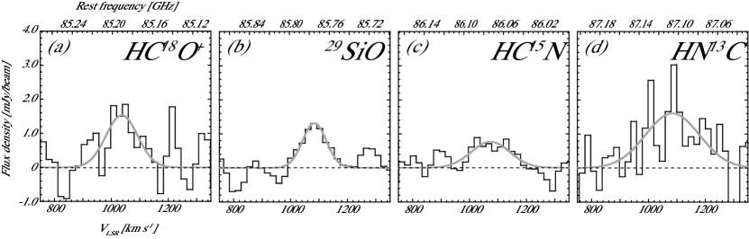
Figure 2: The spectra and Gaussian fitting curves of the first detection or the first observation with the interferometer in NGC 1068 include (a) HC¹⁸O⁺, (b) ²⁹SiO, (c) HC¹⁵N, and (d) HN¹³C. The vertical axis is the flux density per convolved beam. The spatial resolution is 5.$\!{}^{\prime\prime}$0 ($\sim$350 pc) for (a) and (d) centered at the AGN position, and 0.$\!{}^{\prime\prime}$9 ($\sim$60 pc) for (b) and (c) centered at the E-knot position (coordinates are explained in the text of section 3.2). The horizontal axes represent the velocity ($V_{\rm LSR}$; lower) and rest frequency (upper).

Figure  2 shows spectra of the first detection or of new detections with the interferometer in NGC 1068. The molecules detected include (a) HC¹⁸O⁺ ($J$ = 1–0), (b) ²⁹SiO ($J$ = 2–1), (c) HC¹⁵N ($J$ = 1–0), and (d) HN¹³C ($J$ = 1–0). Profiles (a) and (d) were obtained within the circular region with a 5^′′ diameter at the AGN position, which covers approximately the entire structure of the CND. The integrated fluxes of the detected lines are approximately 3$\sigma$ of the noise level. Profiles (b) and (c) were obtained at the E-knot position, with a resolution of 0.$\!{}^{\prime\prime}$9, and the detection levels are more than 4$\sigma$ for these lines.

Wang et al. (2014) and Qiu et al. (2018) have already reported the detection of HC¹⁸O⁺ toward NGC 1068 with the IRAM 30-m single-dish telescope. The calculated peak velocity with Gaussian fitting obtained using ALMA is 1037$\pm$27 km s^-1 (Figure  2(a)), and this value is consistent with that in previous studies. In addition, the line shape, which has several velocity components, is almost identical to that of the IRAM 30-m.

Qiu et al. (2018) reported the detection of H42$\alpha$ at 85.6950 GHz; however, it was not detected around that frequency in this observation. We found line features in the range of 85.75–85.80 GHz (Figure  2(b)), which are close to the frequency of this recombination line. This range is in close agreement with the frequency of ²⁹SiO ($J$ = 2–1, v=0; 85.759144 GHz; Lovas, 2004), and the detection of this isotopologue in NGC 1068 is the first time such detection.

Extragalactic HC¹⁵N has been reported in the Large Magellanic Cloud (LMC) and composite AGN-starburst galaxy NGC 4945 (Chin et al., 1999). However, in NGC 1068, previous line survey observations in the 3-mm band with single-dish telescopes have not yet detected this molecular line (Aladro et al., 2015; Qiu et al., 2018; Takano et al., 2019). The only upper limit reported is $<$115 mK km s^-1 (2$\sigma$) by Wang et al. (2014). In this observation, HC¹⁵N was detected in the peak positions of both the E- and W-knots, which were detected at 3.5–4$\sigma$. The integrated line ratios of HC¹⁴N/HC¹⁵N in LMC and NGC 4945 were reported by Chin et al. (1999) to be 49–69 and 46, respectively. In this work, this ratio at the E-knot position in NGC 1068 is calculated as 64.8$\pm$15.0, which is close to that in the LMC.

HN¹³C in NGC 1068 has been reported by Wang et al. (2014) and Qiu et al. (2018) using the IRAM 30-m telescope. In this study, the integrated flux ratio of HN¹²C/HN¹³C was measured to be 26.4$\pm$8.5, which ranges between 23.3 (Aladro et al., 2013) and 38.1 (Wang et al., 2014). This consistency indicates that HN¹³C is mainly located in the CND with a minor contribution from the SBR.

3.2 Molecular gas distributions

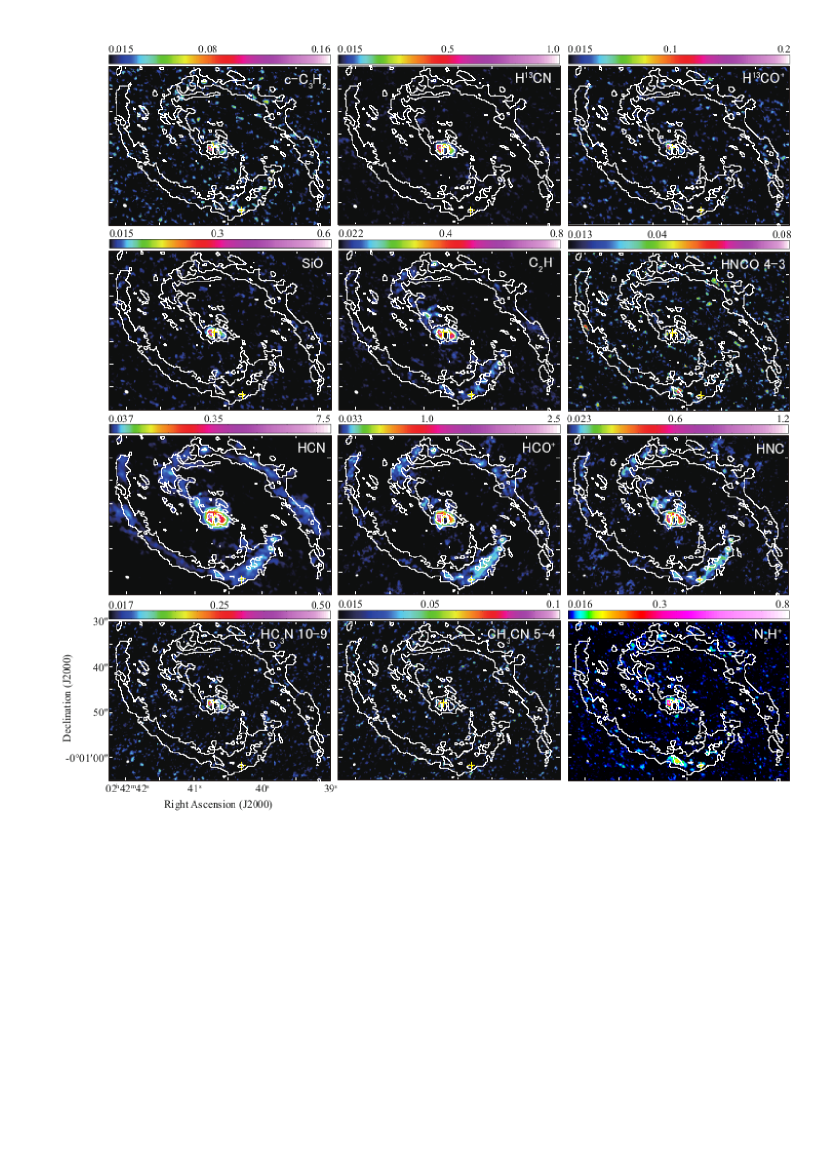
Figure 3: The images of integrated flux (moment-0) for 23 molecular lines, which are clearly detected both in the CND and the SBR in NGC 1068. The unit of the color scale is Jy beam^-1 km s^-1, and the minimum color levels are set to 1$\sigma$ noise level for each molecular line. The contour maps are 3$\sigma$ and 9$\sigma$ of ¹²CO ($J$ = 1–0); the integrated flux indicates a typical gas distribution. The positions of the AGN (Gallimore et al., 2004) and the southwestern region in the SBR (Takano et al., 2014) are indicated using yellow cross marks.

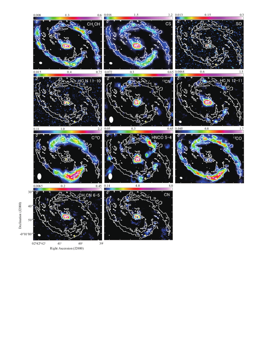
Figure 4: (continued).

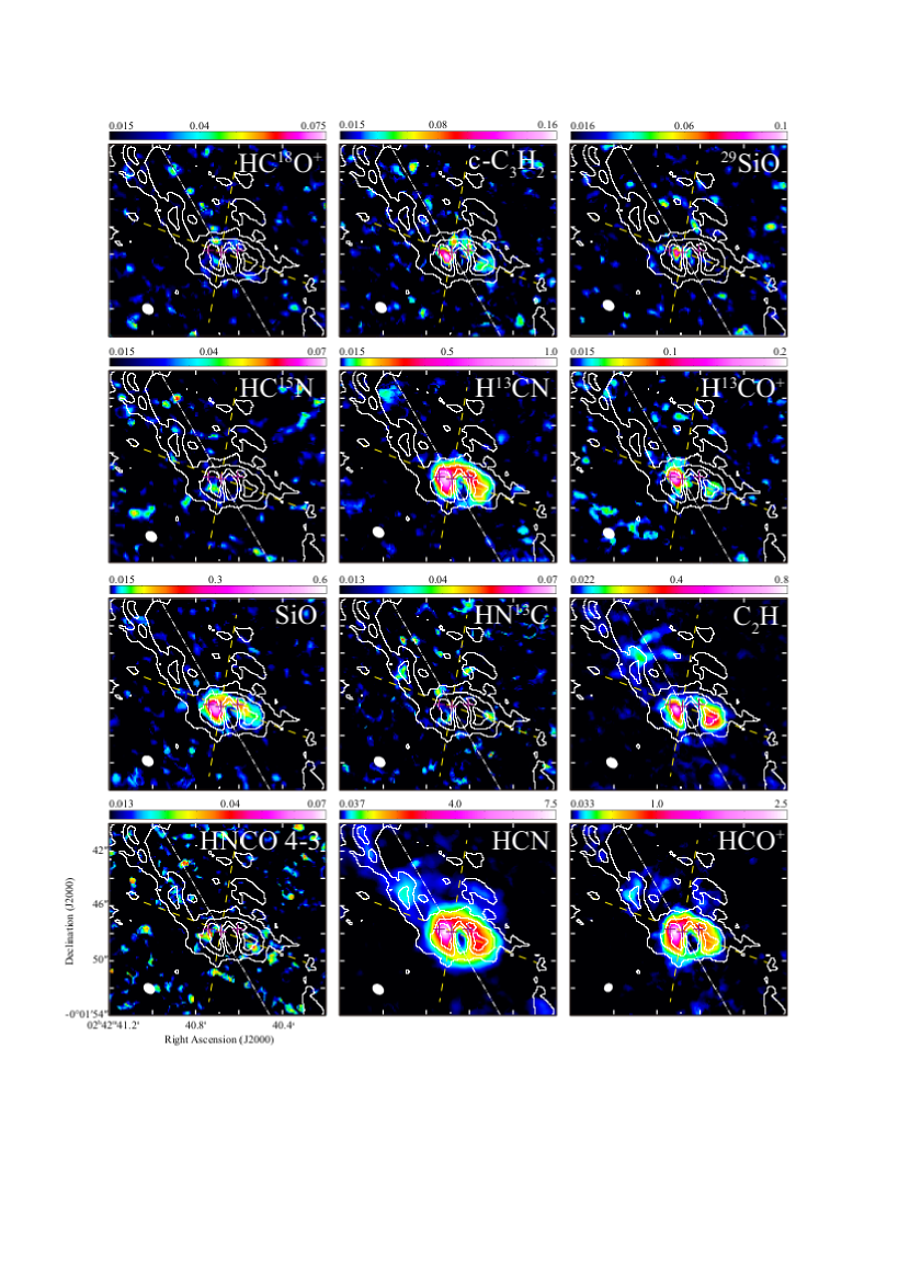
Figure 5: The enlarged integrated flux (moment-0) view of the CND for 23 molecular lines, which are obtained with high spectral resolution (synthesized beam$<$1^′′) and include the newly detected lines (see Section 3.1). The unit of the color scale is Jy beam^-1 km s^-1, and the minimum color levels are set to a 1$\sigma$ noise level for each molecular line. The contour maps are 3$\sigma$, 6$\sigma$, and 12$\sigma$ of ¹²CO ($J$ = 1–0); the integrated flux indicates a typical gas distribution. Three magenta cross marks represent the positions of the E-knot, AGN, and W-knot from the left side (the coordinates are explained in the text of Section 3.2). The dual cone structure with a 30^∘ position angle (dash-dot-dash line) and 40^∘ outer opening angle (dashed-line) from the location of the supermassive black hole is represented in all images (Das et al., 2006).

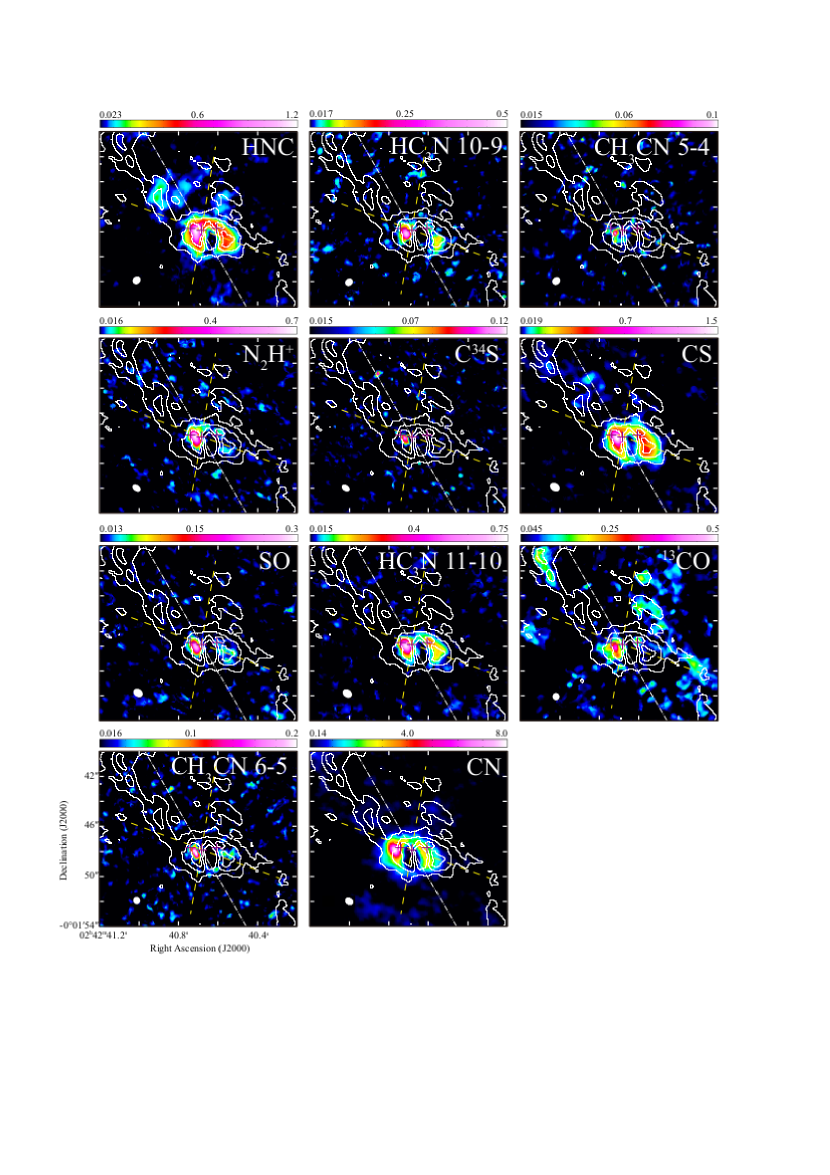
Figure 6: (continued).

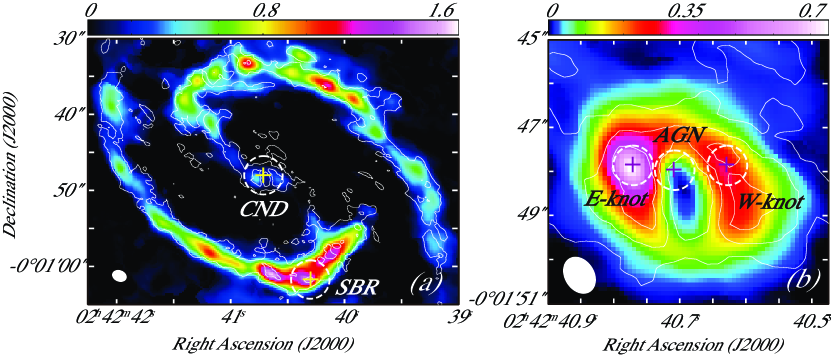
Figure 7: The extracted positions of spectral data are indicated by crosses on (a) the ¹³CO moment-0 map for the CND and SBR, and on (b) the HCN moment-0 map for the AGN, E-, and W-knots. These coordinates are explained in the text of Section 3.2. The contour map shows a ¹²CO distribution (see the captions of Figures 3 and  5). The dashed-line circles represent the convolved beam sizes of 5.$\!{}^{\prime\prime}$0 ($\sim$350 pc) in (a) and 0.$\!{}^{\prime\prime}$9 ($\sim$60 pc) in (b). These beams do not overlap and the samples are spatially independent.

Based on the molecular lines detected in our previous line survey observation with a single-dish telescope (Takano et al., 2019), we obtained the spatial distributions of the major molecular species with ALMA. In this ALMA observation, which ranged from 84–114 GHz, we successfully obtained 21 molecular line distributions for all detected molecular lines using the NRO 45-m telescope. Moreover, non-detected lines with the NRO 45-m telescope, H¹³CO⁺ ($J$ = 1–0) and CH₃CN ($J_{K}$ = 5_K–4_K), were clearly detected and imaged using ALMA. Figures 3 and  4 show the integrated flux (moment-0) as color maps of 23 molecular lines (15 molecular species and four isotopologues) covering the entire central structure, which consists of the CND and SBR. The positions of the AGN (Gallimore et al., 2004) and southwestern region in the SBR (Takano et al., 2014) are indicated using cross marks on all images. The minimum color level for each molecular line was set to a 1$\sigma$ noise level. These levels were estimated from the averaged RMS noise in the region of the emission-free blank sky as typical noise over the map. The overlaid contour map in each image represents the integrated flux of ¹²CO ($J$ = 1–0) obtained during observations 2018.1.01684.S (P.I. T. Tosaki) which exhibited a typical gas distribution. These contours represent the 3$\sigma$ and 9$\sigma$ noise levels. All $uv$ range data are used in the imaging process, and the range is different on an observational basis (see Table 2). Primary beam correction was not applied to any of the integrated flux images (Figures 3–6).

A method was applied to create integrated flux maps with higher S/N ratios compared to the standard process using the immoments task in CASA. The central channel (i.e., the peak velocity) and the number of channels for integration (i.e., the velocity width) of the spectrum are the same for each pixel in the simplest method. However, in the new method, the values are changed on a pixel-by-pixel basis depending on the peak velocity (moment-1) and velocity dispersion ($\sigma$$V$; moment-2) of ¹²CO ($J$ = 1–0) as the template. The detailed procedure of this method will be presented in a separate paper (A. Taniguchi et al. in prep.). The velocity width for integration was calculated using the velocity dispersion of the template spectrum multiplied by an arbitrary factor, and we applied 3$\sigma$$V$ in this work. The peak velocity and velocity width applied to the integrated flux map images are different for each pixel, but these values are common for all molecular lines. For example, the typical peak velocity at the CND is 1100–1150 km s^-1. Those in the eastward and westward SBR regions from the CND are approximately 1000–1050 km s^-1 and 1200–1250 km s^-1, respectively. The typical velocity dispersion in the CND and SBR regions was approximately 80 km s^-1 and 50 km s^-1, respectively.

Although the distributions of ¹³CN, C¹⁸O, and HNCO ($J_{Ka,Kc}$ = 5_0,5–4_0,4) were reported in Takano et al. (2014), and CH₃OH, CS, and ¹³CO were already reported in Tosaki et al. (2017) using the same data, these images are presented again in this paper for completeness. The S/N of these images was drastically improved owing to the new method. In addition, images of SO, HC₃N ($J$ = 11–10; 12–11), and CH₃CN ($J_{K}$ = 6_K–5_K), which are taken in the cycle-0 period, have been reported by Takano et al. (2014). However, these images are presented in this paper again using the newly obtained data in cycle-2 because the spatial resolutions are approximately ten times higher than those of the previous works.

To date, images of the molecular distribution using interferometers covering both the CND and SBR in NGC 1068 have been previously reported. However, these were obtained only for relatively strong emission lines such as those of CO, HCN, HCO⁺, and CS. For ¹²CO see Planesas et al. (1991), Kaneko et al. (1992), Helfer et al. (1995), Schinnerer et al. (2000), Tsai et al. (2012); for ¹³CO see Helfer et al. (1995), Papadopoulos et al. (1996), Tacconi et al. (1997); for C¹⁸O see Papadopoulos et al. (1996). Other references include Tacconi et al. (1994), Helfer et al. (1995), Kohno et al. (2008) for HCN, Kohno et al. (2008) for HCO⁺, and Tacconi et al. (1997), Scourfield et al. (2020) for CS. Observations of other molecules toward this galaxy are quite limited even in the 3-mm band. With the exception of papers reported by our group (Takano et al., 2014; Tosaki et al., 2017; Saito et al., 2022a, b), SiO (Garcia-Burillo et al., 2010; Huang et al., 2022), C₂H (Garcia-Burillo et al., 2017), CS (Scourfield et al., 2020), and HCN, HCO⁺ (Sánchez-García et al., 2022) with ALMA are the only reported studies. Therefore, many of the molecular distribution images obtained in the central region of NGC 1068 are being presented for the first time.

In Figures 3 and  4, the molecules showing a variety of spatial distributions are likely due to the difference in physical/chemical properties between the CND and SBR. The strong emissions of H¹³CN, H¹³CO⁺, SiO, HC₃N, CH₃CN, SO, and ¹³CN are concentrated in the CND, whereas weak emissions were observed in the SBR. The enhancement of these molecules in the CND may be due to the effect of the AGN. In contrast, C¹⁸O and ¹³CO were mainly distributed in the SBR, and were significantly weak in the CND. This feature is well known from previous studies, and we have already discussed it in Takano et al. (2014). Other molecules, cyclic-C₃H₂ (hereafter $c$-C₃H₂), C₂H, HNCO, HCN, HCO⁺, HNC, N₂H⁺, CH₃OH, CS, and CN, are distributed in both the CND and SBR. We find that the emissions of $c$-C₃H₂, HNCO ($J_{Ka,Kc}$ = 4_0,4–3_0,3), and N₂H⁺ in the SBR show particularly clumpy structures without diffuse components at the peak positions of ¹²CO. However, this may be due to an insufficient S/N or missing flux because these emission lines are very weak, especially in the SBR relative to other molecules in this category. In addition, CH₃OH ($J_{K}$ = 2_K–1_K) and HNCO ($J_{Ka,Kc}$ = 5_0,5–4_0,4) exhibit a characteristic distribution in the SBR. These peak positions are clearly different from those of ¹²CO. These molecules may reflect dynamic effects, such as cloud-cloud collisions and/or galaxy dynamics, instead of interstellar mass distribution, because they are known as shock tracers. The distribution of CH₃OH was also analyzed and discussed in Tosaki et al. (2017).

Figures  5 and  6 show enlarged views of the CND. We obtained a clear distribution of 23 molecular lines with a peak S/N$>$5 and a $<$1.0 arcsec resolution. The image size is approximately 15^′′ square ($\sim$1 kpc at a distance of 14.4 Mpc), which is almost the same size as the NRO 45-m telescope main beam around the center of the CND. The three crosses represent the positions of the E-knot, AGN, and W-knot, which were defined by Gallimore et al. (2004) for the AGN and Viti et al. (2014) for the others, from the left side of each image. In addition, the configuration of the biconical outflow model (Das et al., 2006) is indicated in all images. They proposed a biconical structure with a 30^∘ position angle and 40^∘ outer opening angle from the location of the supermassive black hole based on observations of the narrow-line region in NGC 1068 obtained with the Hubble Space Telescope (HST) and the Multi-Element Radio Linked Interferometer Network (MERLIN) radio maps. We expect to find dynamical and chemical effects owing to the interaction between the AGN jet-driven outflow and the galactic disk, as proposed by Garcia-Burillo et al. (2014) and Saito et al. (2022a).

Some molecular lines, H¹³CN, SiO, C₂H, HCN, HCO⁺, HNC, CS, and CN, show a clear ring structure in the CND, similar to the ¹²CO distribution (i.e., the contours). Other molecules were mainly detected in the vicinity of the E- and W-knots. C₂H, HC₃N, and CS show comparable peaks in both knots, but the following molecules are stronger in the E-knot with moderate detections in the W-knot: c-C₃H₂, ²⁹SiO, H¹³CO⁺, CH₃CN, N₂H⁺, C³⁴S, SO, and ¹³CO. There is no stronger molecular line in the W-knot as in the exceptional case of a neutral atomic carbon line (see Saito et al., 2022a). The peak intensity position in the W-knot varies with the molecule. In particular, H¹³CO⁺, HN¹³C, C₂H, HNCO, HC₃N ($J$ = 10–9), and SO peaks are approximately 1.$\!{}^{\prime\prime}$0–1.$\!{}^{\prime\prime}$5 southwest of the ¹²CO ($J$ = 3–2) peak, as defined by Viti et al. (2014). The comparison of these molecular abundances in each knot is discussed in Section 4.

An elongated structure toward the northeast can be seen in C₂H, HCN, HCO⁺, HNC, CS, and CN. This feature is also observed in the ¹²CO distribution. This structure connects the CND to the surrounding SBR. In addition, we found strong spot emissions approximately 5^′′–6^′′ north and 3^′′ east of the AGN position along the central axis of the northeastern outflow for many molecules such as HC¹⁸O⁺, c-C₃H₂, HC¹⁵N, HN¹³C, HNCO, CH₃CN, C³⁴S, and CS. This position coincides with the hot spot of the AGN jet detected with the Very Large Array (VLA) at a wavelength of 6 cm (Gallimore et al., 1996). Das et al. (2006) proposed that there is an interaction between gas in the host galaxy and ionizing radiation in a part of the northeastern outflow. Therefore, these bright spots likely appear because of gas interactions. This position coincides with the bow-shock arc observed in the cold dust map reported by Garcia-Burillo et al. (2014). However, distinctive structures in all the molecules were not found in the southwestern outflow region.

The amount of missing flux for each molecular line is summarized in the third and fourth column of Table 3 as recoverable flux compared with the total fluxes obtained with two single-dish telescopes. The integrated fluxes obtained with the NRO 45-m telescope ($\theta_{\rm mb}$ = 15.$\!{}^{\prime\prime}$2–19.$\!{}^{\prime\prime}$1) and IRAM 30-m telescope ($\theta_{\rm mb}$ = 21$\!{}^{\prime\prime}$–29$\!{}^{\prime\prime}$) were obtained from Takano et al. (2019) and Aladro et al. (2015). The fluxes were recovered by approximately 60–80% for most of the molecules detected in this line survey with the ALMA 12-m antennae. However, several molecules, such as HC₃N ($J$ = 10–9) and N₂H⁺, show recovered fluxes below 40% relative to both single-dish telescopes. The reason for this large missing flux of HC₃N ($J$ = 10–9) could be explained by the fact that the flux obtained for this molecule with the NRO 45-m telescope was not accurate owing to the large noise level and baseline fluctuation (see Nakajima et al., 2018; Takano et al., 2019). For N₂H⁺, the reason for the large missing flux is the maximum recoverable scale of the array configuration (see Section 2).

3.3 Line properties at 350 pc scale

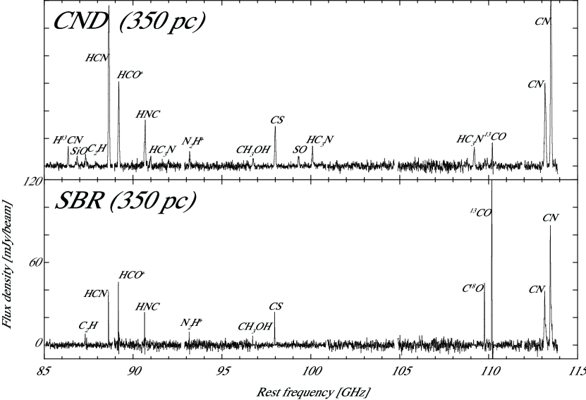
Figure 8: The obtained spectra with spatial resolution of 5.$\!{}^{\prime\prime}$0 ($\sim$350 pc) from 85 to 114 GHz in the CND (upper panel) and the SBR (lower panel). The vertical and horizontal axes are the beam-averaged flux density and rest frequency, respectively. The velocity resolution is 20 km s^-1, and the primary beam correction is applied. The names of major molecular line carriers are indicated above the spectra.

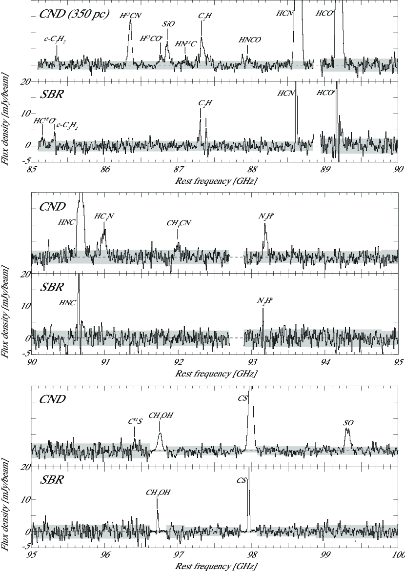
Figure 9: Enlarged spectra with a spatial resolution of 5.$\!{}^{\prime\prime}$0 ($\sim$350 pc) from 85 to 100 GHz in the CND (upper panel) and the SBR (lower panel). The vertical and horizontal axes are the beam-averaged flux density and rest frequency, respectively. The velocity resolution is 20 km s^-1, and the primary beam correction is applied. The shaded regions refer to the range of $\pm$1$\sigma$ noise level. The names of the molecular line carriers, which have a peak flux of more than 1$\sigma$, are indicated above the spectra.

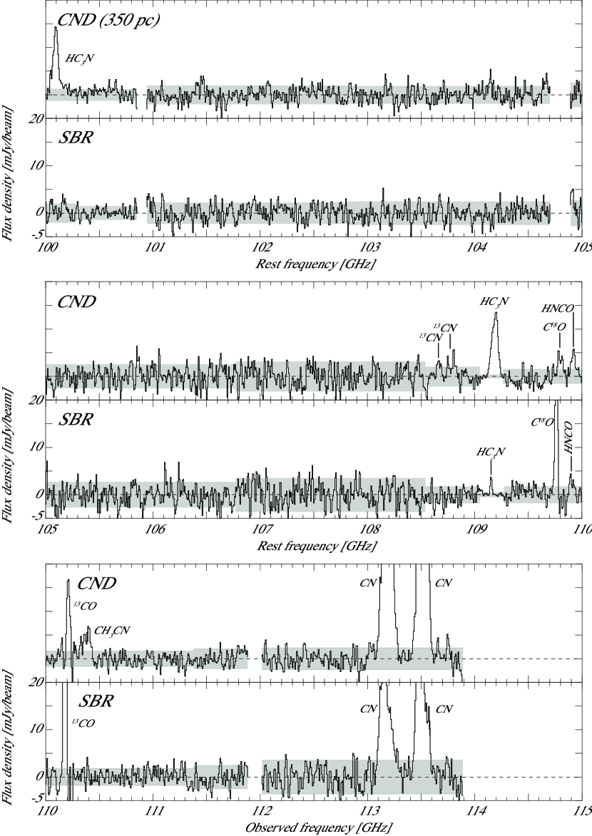
Figure 10: Enlarged spectra with a spatial resolution of 5.$\!{}^{\prime\prime}$0 ($\sim$350 pc) from 100 to 114 GHz in the CND (upper panel) and the SBR (lower panel).

To investigate the differences in the physical/chemical properties of the interstellar medium affected by the AGN and starburst sources, we extracted the line spectra in the AGN and SBR positions with a convolved beam size of 5.$\!{}^{\prime\prime}$0 ($\sim$350 pc). This is the highest matched angular resolution in this line survey (see Table 2). As shown in Figure 7(a), the beam in the AGN position covers the entire structure of the CND, which was covered by an asymmetric elongated ring of 4^′′ $\times$ 2.$\!{}^{\prime\prime}$8, as indicated by Garcia-Burillo et al. (2014).

The spectra from 85 to 114 GHz at these two positions are shown in Figure 8. The velocity resolution was set to 20 km s^-1, and primary beam correction was applied to all spectra (Figures 8–14). To obtain information from the same interstellar gas component among all 24 SPWs (see Table 2), the minimum baseline is standardized for imaging and for extracting spectra. The $uv$ range is used for more than 15 k$\lambda$, which is the largest common minimum $uv$ range of all SPWs (see Table 2).

While more than 15 species, such as HCN, HCO⁺, CO isotopologues, and CN, were detected in both the CND and SBR, the flux density ratios were different between these regions. For example, $R_{{\rm HCN/HCO^{+}}}$ is approximately two at the CND, whereas it is below unity for the SBR. The flux ratios of $R_{{\rm H^{13}CN/CS}}$, $R_{{\rm SiO/CS}}$, and $R_{{\rm HC_{3}N/CS}}$ at the CND (0.4, 0.2, and 0.3–0.4) are significantly larger than those in the SBR ($<$0.07, $<$0.07, and 0.1), despite the fact that the peak fluxes of CS are almost similar at the CND and SBR. The lines of the CO isotopologues are very weak in the CND.

Figures 9 and 10 show the detailed spectra from 85 to 114 GHz at 5 GHz intervals. Molecular line identification is only performed for peak fluxes above the 1$\sigma$ noise level (shaded regions in the images) by eye, and the results are displayed with the names of the molecular carriers of lines. The integrated fluxes of each molecule are shown in the 5th and 6th columns of Table 3, and the non-detected lines (peak flux $<$1$\sigma$) are shown as the upper limit.

3.4 Line properties at 60 pc scale

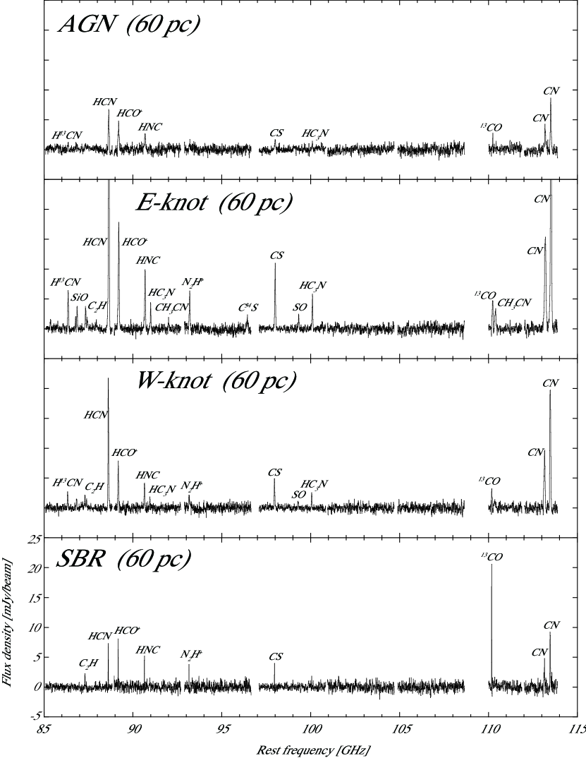
Figure 11: Obtained spectra with a spatial resolution of 0.$\!{}^{\prime\prime}$9 ($\sim$60 pc) from 85 to 114 GHz in the AGN, the E-knot, the W-knot, and the SBR (from top down). The vertical and horizontal axes are the beam-averaged flux density and rest frequency, respectively. The velocity resolution is 20 km s^-1, and the primary beam correction is applied. The names of major molecular line carriers are indicated above the spectra.

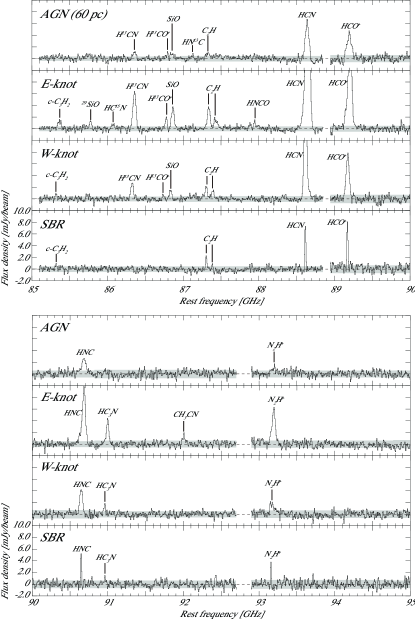
Figure 12: Enlarged spectra with a spatial resolution of 0.$\!{}^{\prime\prime}$9 ($\sim$60 pc) from 85 to 95 GHz in four regions (see the caption of Figures 11). The vertical and horizontal axes are the beam-averaged flux density and rest frequency, respectively. The velocity resolution is 20 km s^-1, and the primary beam correction is applied. The shaded regions represent the range of the $\pm$1$\sigma$ noise level. The names of the molecular line carriers, for which the peak flux is more than 1$\sigma$, are indicated above the spectra.

Figure 13: Enlarged spectra with a spatial resolution of 0.$\!{}^{\prime\prime}$9 ($\sim$60 pc) from 95 to 105 GHz in four regions (see the caption of Figures 11).

Figure 14: Enlarged spectra with a spatial resolution of 0.$\!{}^{\prime\prime}$9 ($\sim$60 pc) from 105 to 114 GHz in four regions (see the caption of Figures 11).

To determine the difference in physical/chemical properties within the CND, that is, the central position (AGN position), E-knot, and W-knot, we extracted a spectrum from the data cubes at these positions as well as the SBR with a convolved beam size of 0.$\!{}^{\prime\prime}$9 ($\sim$60 pc). This is the lowest common value among the observations of the extended antenna configuration (greater than 1600 m; Table 1). As shown in Figure 7(b), the beams at the E-knot, AGN, and W-knot positions do not overlap. However, the diffuse and extended molecular gas components around the knots likely contaminate the spectrum at the AGN position. We believe that our AGN spectrum is more or less contaminated, especially by the neighboring E-knot. Thus, our AGN spectrum does not originate solely from the AGN torus (Garcia-Burillo et al., 2016; Imanishi et al., 2018, 2020). In such a case, the source size is smaller than the convolved beam size; thus, the beam-averaged integrated flux and the column density may be underestimated. Because we would like to obtain the line properties under the same conditions at all sampling positions without arbitrary assumptions, the beam-filling factor is assumed to be unity.

The spectra from 85 to 114 GHz at these four positions are shown in Figure 11. The velocity resolution was set to 20 km s^-1, and primary beam correction was applied for all images. The $uv$ range is used for more than 15 k$\lambda$, which is the same as that in the previous section. Figures 12,  13, and  14 show the detailed spectra from 85 GHz to 114 GHz at 5 GHz intervals. The integrated fluxes of the detected lines are shown from the 7th to 10th columns of Table 3, and the non-detected lines (peak flux $<$1$\sigma$) are shown in the upper limit.

Table 3: Recovered and integrated flux for each molecular line.

Frequencya	Molecule	Recovery			$\int$flux$dv$ (Jy beam-1 km s-1)
(GHz)	(Transition)	(%)			5.$\!{}^{\prime\prime}$0 resolution			0.$\!{}^{\prime\prime}$9 resolution
		NROb	IRAMc		CND	SBR		AGN	E-knot	W-knot	SBR
85.162223	HC18O+ (1–0)	—	—		0.23$\pm$0.09d	0.36$\pm$0.11		$<$0.02	$<$0.02	$<$0.03	$<$0.03
85.338894	c-C3H2 (21,2–10,1)	80$\pm$17	—		0.40$\pm$0.09	0.51$\pm$0.11		0.09$\pm$0.02	0.22$\pm$0.03	0.09$\pm$0.02	0.08$\pm$0.03d
85.759194	29SiO (20–10)	—	—		0.33$\pm$0.08	$<$0.11		0.10$\pm$0.02	0.15$\pm$0.02	0.08$\pm$0.02	$<$0.03
86.054966	HC15N (1–0)	—	—		$<$0.1	$<$0.11		$<$0.03	0.13$\pm$0.03	0.07$\pm$0.02	$<$0.03
86.339921	H13CN (1–0)	88$\pm$17	62$\pm$10		2.67$\pm$0.13	$<$0.11		0.22$\pm$0.03	1.06$\pm$0.03	0.40$\pm$0.03	$<$0.03
86.754288	H13CO+ (1–0)	—	—		0.53$\pm$0.1	$<$0.11		0.11$\pm$0.02	0.22$\pm$0.02	0.07$\pm$0.03d	$<$0.03
86.846985	SiO (2–1)	108$\pm$31	52$\pm$10		1.40$\pm$0.12	$<$0.11		0.16$\pm$0.03	0.58$\pm$0.03	0.2$\pm$0.03	$<$0.03
87.090825	HN13C (1–0)	—	—		0.28$\pm$0.09	$<$0.09		0.08$\pm$0.03d	$<$0.03	0.08$\pm$0.03d	$<$0.03
87.316898	C2H (1–0)	138$\pm$9	54$\pm$2		2.14$\pm$0.14	1.17$\pm$0.13		0.41$\pm$0.06	0.92$\pm$0.05	0.55$\pm$0.06	0.22$\pm$0.04
87.925237	HNCO (40,4–30,3)	45$\pm$12	56$\pm$89		0.73$\pm$0.13	0.14$\pm$0.09d		0.17$\pm$0.03	0.23$\pm$0.03	$<$0.04	0.1$\pm$0.03
88.631602	HCN (1–0)	108$\pm$3	60$\pm$1		28.04$\pm$0.14	3.05$\pm$0.09		1.19$\pm$0.04	8.42$\pm$0.05	3.31$\pm$0.05	0.45$\pm$0.02
89.188525	HCO+ (1–0)	118$\pm$6	67$\pm$1		14.0$\pm$0.18	2.75$\pm$0.11		1.19$\pm$0.06	3.69$\pm$0.06	1.27$\pm$0.06	0.45$\pm$0.03
90.663568	HNC (1–0)	147$\pm$12	63$\pm$3		7.39$\pm$0.19	1.65$\pm$0.11		0.73$\pm$0.07	1.77$\pm$0.05	0.68$\pm$0.06	0.26$\pm$0.03
90.979023	HC3N (10–9)	13$\pm$4	50$\pm$17		2.20$\pm$0.23	0.23$\pm$0.09d		0.18$\pm$0.06d	0.75$\pm$0.06	0.21$\pm$0.04	0.09$\pm$0.03d
91.987088	CH3CN (5K–4K)	—	—		0.84$\pm$0.17	$<$0.15		$<$0.06	0.25$\pm$0.05	$<$0.04	$<$0.04
93.173977	N2H+ (1–0)	24$\pm$5	17$\pm$1		1.55$\pm$0.16	0.40$\pm$0.24d		0.26$\pm$0.05	1.10$\pm$0.06	0.43$\pm$0.06	0.15$\pm$0.03
96.412950	C34S (2–1)	—	—		0.39$\pm$0.14d	$<$0.13		$<$0.05	0.45$\pm$0.07	$<$0.05	$<$0.04
96.744550	CH3OH (2K–1K)	37$\pm$7	100$\pm$17		1.12$\pm$0.04	0.44$\pm$0.04
97.980953	CS (2–1)	56$\pm$2	81$\pm$2		6.78$\pm$0.04	1.68$\pm$0.03
		83$\pm$5	60$\pm$3					0.32$\pm$0.04	1.74$\pm$0.04	0.70$\pm$0.04	0.17$\pm$0.02
99.02296	H40$\alpha$	—	—		$<$0.08	$<$0.13		$<$0.03	$<$0.03	$<$0.03	0.08$\pm$0.03d
99.299870	SO (32–21)	84$\pm$21	84$\pm$12		1.51$\pm$0.12	$<$0.18
		60$\pm$26	41$\pm$17					$<$0.04	0.36$\pm$0.04	0.17$\pm$0.03	$<$0.04
100.076385	HC3N (11–10)	75$\pm$14	87$\pm$6		2.88$\pm$0.12	0.24$\pm$0.18d
		81$\pm$22	66$\pm$14					0.17$\pm$0.03	0.84$\pm$0.04	0.29$\pm$0.03	0.08$\pm$0.02
108.651297	13CN (1–0)	58$\pm$9	—		0.65$\pm$0.19	$<$0.16
109.173638	HC3N (12–11)	61$\pm$5	156$\pm$8		2.49$\pm$0.03	0.21$\pm$0.05
109.782173	C18O (1–0)	44$\pm$3	55$\pm$2		0.65$\pm$0.14	3.32$\pm$0.16
109.905753	HNCO (50,5–40,4)	43$\pm$8	—		0.72$\pm$0.14	0.27$\pm$0.16d
110.201354	13CO (1–0)	61$\pm$1	61$\pm$1		1.67$\pm$0.14	9.09$\pm$0.16
		32$\pm$1	61$\pm$2					0.17$\pm$0.04	0.79$\pm$0.04	0.38$\pm$0.06	1.06$\pm$0.04
110.383500	CH3CN (6K–5K)	115$\pm$23	49$\pm$35		1.11$\pm$0.16	$<$0.16
		54$\pm$26	23$\pm$29					0.10$\pm$0.04d	0.64$\pm$0.05	0.26$\pm$0.06	0.11$\pm$0.03
113.191279	CN (1–0)	141$\pm$4	103$\pm$3		14.89$\pm$0.21	8.49$\pm$0.32		0.79$\pm$0.06	4.06$\pm$0.08	1.87$\pm$0.06	0.47$\pm$0.06
113.490970	CN (1–0)	154$\pm$3	87$\pm$1		27.57$\pm$0.21	13.09$\pm$0.32		1.24$\pm$0.05	7.85$\pm$0.09	3.29$\pm$0.06	0.85$\pm$0.05

Note. — ^a Rest frequencies are referenced in Lilley & Palmer (1968) for the recombination line and Lovas (2004) for others. ^b Recovery fluxes with the NRO 45-m telescope were calculated based on Takano et al. (2019). ^c Recovery fluxes with the IRAM 30-m telescope were calculated based on Aladro et al. (2015). ^d Low S/N ($<$3$\sigma$).

3.5 Estimation of column densities

Table 4: Column densities of each molecule.

Molecule	$T_{\rm rot}$ (K)		$N_{\rm mol}$ (cm-2)
				5.$\!{}^{\prime\prime}$0 resolution			0.$\!{}^{\prime\prime}$9 resolution
	CND	SBR		CND	SBR		AGN	E-knot	W-knot	SBR
HC18O+	15$\pm$5	10$\pm$5		2.0${}^{+1.4}_{-1.1}$(12)	2.5${}^{+1.7}_{-1.1}$(12)		$<$5.4(12)	$<$5.4(12)	$<$8.1(12)	$<$6.4(12)
cyclic-C3H2	15$\pm$5	10$\pm$5		2.4${}^{+1.7}_{-1.1}$(13)	2.1${}^{+1.7}_{-1.0}$(13)		1.7${}^{+1.2}_{-0.8}$(14)	4.1${}^{+2.3}_{-1.7}$(14)	1.7${}^{+1.2}_{-0.8}$(14)	1.0${}^{+1.1}_{-0.6}$(14)
29SiO	15$\pm$5	10$\pm$5		4.6${}^{+2.4}_{-1.9}$(12)	$<$1.2(12)		4.2${}^{+2.0}_{-1.6}$(13)	6.5${}^{+2.6}_{-2.1}$(13)	3.7${}^{+1.9}_{-1.5}$(13)	$<$1.0(13)
HC15N	15$\pm$5	10$\pm$5		$<$1.3(12)	$<$1.3(12)		$<$1.4(13)	5.6${}^{+3.0}_{-2.3}$(13)	3.0${}^{+1.8}_{-1.4}$(13)	$<$1.1(13)
H13CN	15$\pm$5	10$\pm$5		3.8${}^{+1.1}_{-1.0}$(13)	$<$1.2(12)		9.7${}^{+3.8}_{-3.1}$(13)	4.7${}^{+1.2}_{-1.1}$(14)	1.7${}^{+0.6}_{-0.5}$(14)	$<$1.0(13)
H13CO+	15$\pm$5	10$\pm$5		4.4${}^{+2.0}_{-1.6}$(12)	$<$7.1(11)		2.7${}^{+1.3}_{-1.0}$(13)	5.6${}^{+1.9}_{-1.6}$(13)	1.8${}^{+1.4}_{-1.0}$(13)	$<$6.0(12)
SiO	15$\pm$5	10$\pm$5		1.9${}^{+0.6}_{-0.5}$(13)	$<$1.2(12)		6.7${}^{+3.0}_{-2.4}$(13)	2.4${}^{+0.7}_{-0.6}$(14)	8.2${}^{+3.4}_{-2.7}$(13)	$<$9.8(12)
HN13C	15$\pm$5	10$\pm$5		3.7${}^{+2.3}_{-1.7}$(12)	$<$9.3(11)		3.2${}^{+2.2}_{-1.6}$(13)	$<$1.2(13)	3.5${}^{+2.3}_{-1.7}$(13)	$<$9.6(12)
C2H	15$\pm$5	10$\pm$5		4.4${}^{+1.4}_{-1.2}$(14)	1.9${}^{+0.8}_{-0.5}$(14)		2.6${}^{+1.1}_{-0.9}$(15)	5.8${}^{+1.7}_{-1.5}$(15)	3.5${}^{+1.3}_{-1.0}$(15)	1.1${}^{+0.6}_{-0.4}$(15)
HNCO	9.9${}^{+0.1}_{-5.8}$	10$\pm$5		1.0${}^{+0.1}_{-0.6}$(14)	1.3${}^{+3.5}_{-0.8}$(13)		3.6${}^{+4.3}_{-0.6}$(14)	4.9${}^{+5.4}_{-0.6}$(14)	$<$8.4(13)	2.0$\pm$0.6(14)
HCN	15$\pm$5	10$\pm$5		3.6$\pm$0.8(14)	3.1${}^{+0.8}_{-0.6}$(13)		4.7${}^{+1.3}_{-1.1}$(14)	3.4${}^{+0.8}_{-0.7}$(15)	1.3$\pm$0.3(15)	1.4${}^{+0.4}_{-0.3}$(14)
HCO+	15$\pm$5	10$\pm$5		1.0${}^{+0.3}_{-0.2}$(14)	1.5${}^{+0.5}_{-0.4}$(13)		2.3${}^{+0.7}_{-0.6}$(14)	8.1${}^{+2.2}_{-2.0}$(14)	2.8${}^{+0.9}_{-0.8}$(14)	7.5${}^{+2.3}_{-1.9}$(13)
HNC	15$\pm$5	10$\pm$5		8.4${}^{+2.2}_{-1.9}$(13)	1.5${}^{+0.4}_{-0.3}$(13)		2.6${}^{+0.9}_{-0.7}$(14)	6.2${}^{+1.6}_{-1.5}$(14)	2.4${}^{+0.8}_{-0.7}$(14)	7.3${}^{+1.9}_{-1.3}$(13)
HC3N	16.7${}^{+3.9}_{-3.1}$	10$\pm$5		5.9${}^{+1.5}_{-0.8}$(13)	0.9${}^{+6.0}_{-0.4}$(13)		1.4${}^{+0.7}_{-0.5}$(14)	5.9${}^{+1.3}_{-0.8}$(14)	1.6${}^{+0.6}_{-0.4}$(14)	0.9${}^{+2.0}_{-0.3}$(14)
CH3CN	11.5${}^{+0.7}_{-0.2}$	10$\pm$5		5.5${}^{+4.4}_{-1.5}$(12)	$<$1.2(12)		1.9$\pm$0.8(13)	1.2${}^{+0.0}_{-0.1}$(14)	5.0$\pm$0.1(13)	2.2$\pm$0.6(13)
N2H+	15$\pm$5	10$\pm$5		1.3$\pm$0.4(13)	2.6${}^{+0.7}_{-0.4}$(12)		6.6${}^{+3.0}_{-2.4}$(13)	2.8${}^{+0.8}_{-0.7}$(14)	1.1$\pm$0.4(14)	3.1${}^{+0.8}_{-0.5}$(13)
C34S	15$\pm$5	10$\pm$5		8.7${}^{+5.8}_{-4.3}$(12)	$<$2.3(12)		$<$3.5(13)	3.1${}^{+1.3}_{-1.0}$(14)	$<$3.5(13)	$<$2.2(13)
CH3OH	15$\pm$5	10$\pm$5		2.7${}^{+1.1}_{-1.7}$(14)	7.6${}^{+6.4}_{-5.0}$(13)
CS	12.6$\pm$0.2	10.5${}^{+0.8}_{-0.6}$		1.4$\pm$0.03(14)	3.0${}^{+0.7}_{-0.3}$(13)		2.0$\pm$0.3(14)	1.1$\pm$0.03(15)	4.4$\pm$0.3(14)	9.7${}^{+2.2}_{-0.9}$(13)
SO	15$\pm$5	10$\pm$5		1.0${}^{+0.4}_{-0.3}$(14)	$<$9.1(12)		$<$8.4(13)	7.6${}^{+2.9}_{-2.6}$(14)	3.7${}^{+1.7}_{-1.4}$(14)	$<$6.2(13)
13CN	15$\pm$5	10$\pm$5		1.7${}^{+0.9}_{-0.7}$(14)	$<$3.4(12)
C18O	13.9${}^{+3.1}_{-2.0}$	8.0$\pm$0.3		2.8${}^{+1.3}_{-1.0}$(15)	1.1${}^{+0.3}_{-0.1}$(16)
13CO	16.7${}^{+1.2}_{-1.0}$	8.5$\pm$0.1		7.6${}^{+0.4}_{-0.3}$(15)	3.0$\pm$0.04(16)		5.5${}^{+2.8}_{-1.8}$(16)	2.6${}^{+0.7}_{-0.4}$(17)	1.3${}^{+0.5}_{-0.3}$(17)	2.1$\pm$0.02(17)
CN	15$\pm$5	10$\pm$5		9.5${}^{+7.8}_{-1.8}$(14)	4.0${}^{+0.9}_{-0.3}$(14)		1.4${}^{+0.4}_{-0.3}$(15)	8.2${}^{+1.8}_{-1.6}$(15)	3.6${}^{+0.8}_{-0.7}$(15)	7.5${}^{+1.7}_{-0.6}$(14)

The column densities ($N_{\rm mol}$) of each molecule were estimated under the assumption of local thermodynamic equilibrium (LTE), and the estimated results are listed in Table 4. In the estimation, the rotational temperatures ($T_{\rm rot}$) and column densities are calculated using the rotation diagram approach under the assumption that all lines are optically thin and that a single excitation temperature characterizes all transitions (e.g., Goldsmith & Langer, 1999). The assumption of LTE, especially in CND, may not be correct because the environment of this region is expected to be significantly affected by strong emissions and/or outflow from the AGN. However, this assumption is the simplest and most commonly used method for estimating molecular abundance. In addition, it allows us a direct comparison with similar studies in the literature (e.g., Martín et al., 2006; Bayet et al., 2009; Aladro et al., 2013).

Because almost all the detected molecules in this work only show a single transition in the 3-mm band, we assume that $T_{\rm rot}$ in the CND (also in the AGN and the E- and W-knots) and that in the SBR are 15$\pm$5 K and 10$\pm$5 K, respectively. These values were determined based on the average of the previous ALMA observations, and the temperatures in the CND and the SBR were significantly different (Nakajima et al., 2015). Derived averaged rotational temperatures among a few molecules with two line detections (Figure 20 in the Appendix) are 13.6 K and 9.0 K toward the CND and the SBR, respectively. Therefore, we believe that the assumed $T_{\rm rot}$ values in the CND and SBR are reasonable. Note that the $T_{\rm rot}$ is a lower limit estimate for kinetic temperature ($T_{\rm kin}$) in general, and the value of $T_{\rm rot}$ is significantly smaller than that of $T_{\rm kin}$ in many cases. In fact, several works derived $T_{\rm kin}$ in the CND with non-LTE analysis, and they derived at least a few hundred kelvins from CO, HCN, HCO⁺, CS, SiO, and HNCO (Viti et al., 2014; Scourfield et al., 2020; Butterworth et al., 2022; Huang et al., 2022).

The column densities of CS, HCN, and HCO⁺ using non-LTE analysis have been reported in previous works. We compare these reported values and our estimations to validate the assumption of LTE analysis. For CS, Scourfield et al. (2020) reported $N$(CS) using RADEX (van der Tak et al., 2007) and UCLCHEM (Holdship et al., 2017) codes. As a result, $N$(CS) in the CND and SBR only from RADEX is consistently compared with our LTE results (see Table 5 in Scourfield et al. 2020). However, $N$(CS) in the SBR from both UCLCHEM and RADEX is larger than our results (see Table 6 in Scourfield et al., 2020). For HCN and HCO⁺, $N$(HCN) and $N$(HCO⁺) in both the CND and SBR from RADEX are significantly large (more than one order of magnitude) relative to the LTE analysis (see Table 6 in Butterworth et al., 2022). If the analysis with the LTE assumption in this work underestimates the column densities, the possibilities of this reason are the effect of optical depth, especially HCN, described above, and a missing flux in this ALMA band-3 observation using only the 12-m main array.

The optical depth of some major molecules with the possibility of being optically thick using the single-dish telescope was reported in the previous research (see Table 2 in Nakajima et al., 2018). Based on this result, ¹²CO, HCN, and CN are optically thick in the case of the beam size of $\sim$1 kpc. Note that ¹²CO is not included in this work. Thus, we estimate the optical depth of these molecules in ALMA observations. The optical depth of HCN is estimated using an assumption of a ¹²C/¹³C ratio ($\sim$38; Tang et al., 2019), and the values with 60 and 350 pc are 7.8 and 3.7, respectively. For CN, the value is estimated to be about 0.1 with both 60 and 350 pc using the intensity ratio of the hyperfine structure (Skatrud et al., 1983). Therefore, HCN is optically thick, and the column density is possibly underestimated. We do not use HCN but mainly H¹³CN to discuss molecular abundance in this paper.

Figure 15: Comparison of column densities of each molecule in (a) 350 pc scale and (b) 60 pc scale. The bar graphs in red, blue, green, and black are for the CND (or AGN), the E-knot, the W-knot, and the SBR, respectively. The order of molecules is arranged in descending order from left to right based on the column density toward CND in (a) or AGN in (b). Arrows indicate upper limits.

4 Discussion

Figure 16: Fractional abundances relative to CS in (a) the 350 pc scale and (b) the 60 pc scale. Ratios over unity, which is indicated by the bold dashed line, represents the enhancement of molecular abundances relative to CS. White arrows indicate the upper limits of the relative abundances. The order of the molecules is arranged in descending order from left to right based on the difference between the CND and the SBR for (a) and between the AGN and the SBR for (b). Therefore, the molecules on the left side of CS are enhancements in the CND (or AGN) compared with the SBR; in contrast, those on the right side of CS are enhancements in the SBR. Note that C³⁴S, SO, HC¹⁵N, and HC¹⁸O⁺ are not detected in both the CND (or AGN) and SBR.

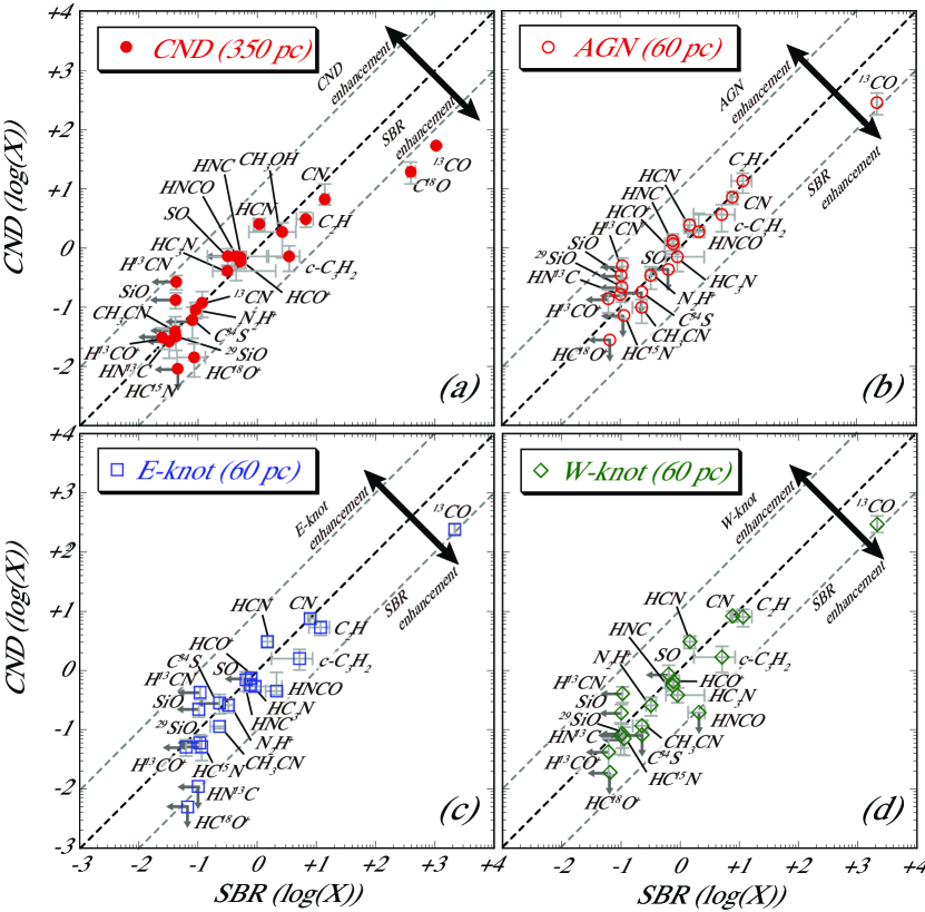
Figure 17: Plots of the fractional abundances relative to CS (a) between CND and SBR with the 350 pc scale, (b) between AGN and SBR with the 60 pc scale, (c) between E-knot and SBR with the 60 pc scale, and (d) between W-knot and SBR with the 60 pc scale. These results represent the abundance correlation between the CND and the SBR. Plots above the bold dashed line represent the enhanced molecules and plots below represent deficient ones in the CND (or AGN).

In this section, we discuss primarily the physical and chemical effects of the AGN on molecular composition and abundance. First, $N_{\rm mol}$ of each molecule and the fractional abundances relative to CS in the CND were compared with those in the SBR. Next, we investigated the difference between the fractional abundances for those obtained with ALMA (spatial resolutions of 60 pc and 350 pc) and the NRO 45-m single-dish telescope ($\sim$1.2 kpc) because it is expected that the higher the resolution, the more clear the effect of the AGN.

4.1 Column densities in the CND vs. SBR

Figure 15 shows the column density of each molecule with spatial resolutions of 350 pc and 60 pc in the CND and SBR. The order of molecules is arranged in descending order from left to right based on $N_{\rm mol}$ toward the CND (350 pc scale) in Figure 15(a), and toward the AGN (60 pc scale) in (b).

At the 350 pc scale, column densities in the CND are systematically higher than those in the SBR, except for ¹³CO, C¹⁸O, and HC¹⁸O⁺. Note that the difference in HC¹⁸O⁺ between the CND and SBR is within the error bar. At the 60 pc scale, column densities in the AGN are systematically higher than those in the SBR, except for ¹³CO. This feature is consistent with the single-dish measurements reported in the literature (e.g., Nakajima et al., 2018). There are no molecules with a higher density in the AGN position than in the E- and/or W- knots. We believe that the dense molecular torus at the AGN position, whose density may be close to that of the knot regions reported by Garcia-Burillo et al. (2016) and Imanishi et al. (2018), is not significant in this observation. In addition, one of the reasons for the lower column densities could be the effect of the beam-filling factor (see Section 3.4). None of the molecules detected in either knot has a higher $N_{\rm mol}$ in the W-knot than in the E-knot in the 60 pc scale except for HN¹³C. The high value for HN¹³C in the W-knot is not significant because the detection is judged with low-S/N (see Table 3). Saito et al. (2022a) reported the integrated intensity map of atomic carbon [C$\mathrm{I}$], and that in the W-knot is higher than that in the E-knot owing to the effect of the AGN jet and outflow. In this work, it is difficult to identify this effect because the samples are only at three positions, and these are too discrete. In a recent study, Saito et al. (2022b) also discussed the effect on molecules using a principal component analysis.

4.2 Fractional abundances relative to CS

Fractional abundances in the CND and SBR at 350 pc and 60 pc resolution are shown in Figure 16 as a column graph, and Figure 17 as a scatter plot. The molecule used for the normalization of abundance was CS, which is one of the best tracers of dense gas because of its high critical density. Scourfield et al. (2020) described the chemistry and excitation in individual regions located in the CND and the SBR in NGC 1068 based on the multi-transitions of CS with ALMA. In addition, fractional abundance with respect to CS is useful for comparing different chemical compositions because CS is known to show a slight variation in abundance among different types of galaxies such as starbursts, AGNs, ULIRGs, and normal galaxies (Martín et al., 2009). Moreover, Saito et al. (2022b) reported that the distribution of CS in NGC 1068 is one of the molecules that has little relation to the AGN-driven outflow. This indicates that the CS abundance is likely to be less sensitive to density variations and dissociation.

The abundant molecules in the CND with a 350 pc scale and in the AGN with a 60 pc scale relative to the SBR are in good agreement; thus, significant differences were not found based on these figures. H¹³CN, SiO, HCN, and H¹³CO⁺ were enhanced in the entirety of all CND and AGN positions. In fact, HCN (4–3)/CS (2–1 and 7–6) in the CND and AGN position are significantly higher than that in the SBR with ALMA high-resolution ($\sim$40 pc) observations (Butterworth et al., 2022). The enhancement of these molecules is possibly due to a shock by the AGN outflow. Because the line intensity ratio is increasing in high-velocity components (i.e., $>$200 km s^-1; broad wing component) than that in the central velocity components in the case of the HCN/CS intensity ratio. Unfortunately, due to low S/N, line ratios for the high-velocity components for H¹³CN, SiO, and H¹³CO⁺ cannot be calculated. In contrast, ¹³CO was enhanced in the SBR with both spatial resolutions. No clear trend can be found in the other molecules because they are not much different owing to the large error bars or are not detected in the AGN and/or SBR.

The abundance of CN, which is known as a possible tracer of X-ray dominated regions (XDRs) proposed in theoretical studies (e.g., Maloney et al., 1996; Meijerink & Spaans, 2005; Meijerink et al., 2007), is one of the highest among all detected molecules in the CND and AGN. Thus, strong X-ray radiation from the AGN was expected. This feature was also described in Garcia-Burillo et al. (2010). However, CN in the SBR is also abundant based on our line survey, and the high abundance of CN is not only due to high X-ray flux, but also due to UV radiation (i.e., photon-dominated regions; PDRs) (Jansen et al., 1995). We have already discussed the abundance of CN toward NGC 1068 in a previous work using single-dish observations (Nakajima et al., 2018), and this result does not change with the observational scale.

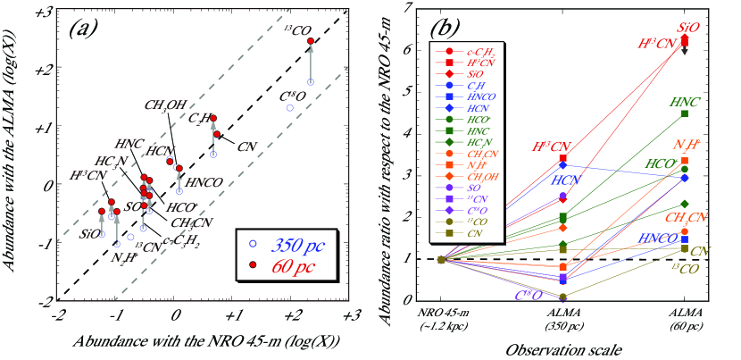
Figure 18: (a) Plot of the fractional abundances with respect to CS between the observation with ALMA and the NRO 45-m telescope. Blue open circles and red filled circles represent the abundances in the CND with the 350 pc scale and those in the AGN with the 60 pc scale, respectively. These results represent the abundance correlation between the 350 pc and 1.2 kpc scales, and between the 60 pc and 1.2 kpc scales. Plots with the bold dashed line represent the same abundance without dependence on the observational scale. Arrows indicate increasing or decreasing abundance from 350 pc to the 60 pc scale. (b) Fractional abundances with respect to CS normalized by the NRO 45-m telescope traced on a 1.2 kpc scale. The bold dashed line represents an abundance ratio of unity.

4.3 Comparison with the abundance using the single-dish telescope

The NRO 45-m telescope was used to obtain molecular abundances toward the central region of NGC 1068 with an approximate 1.2 kpc scale (Nakajima et al., 2018; Takano et al., 2019). Figure 18 shows the dependence of the scale on the molecular abundance with respect to CS by comparing ALMA results with those of the NRO 45-m telescope. It is expected that the smaller the beam size (i.e., from 1.2 kpc through 350 pc to 60pc), the clearer the effect of the AGN as an abundance enhancement or deficient. The enhancements or deficiencies are plotted above or below the lines with a slope of 1 in Figure 18(a) and lines with a ratio of 1 in (b), respectively.

In these figures, ¹³CO and C¹⁸O with both 350 pc and 60 pc scales show low abundance values relative to the 1.2 kpc scale at first sight. This means the abundance with 1.2 kpc is the highest among these observational scales. The molecular gas of the CO isotopologues is distributed in the interarm region between the CND and the SBR (d $>$350 pc), as shown in Tosaki et al. (2017), while the NRO 45-m telescope detected the emission from the components. Except for these CO isotopologues, the fractional abundance of almost all molecules at the 350 pc scale is consistent with those at the 1.2 kpc scale. The abundances of CH₃OH, H¹³CN, SiO, and HCN are slightly higher (ratio $>$2), as shown in Figure 18(b). In contrast, a different trend of plots with 60 pc is clearly observed for some molecules. SiO, H¹³CN, and HNC are significantly enhanced, while HCO⁺, N₂H⁺, C₂H, HCN, c-C₃H₂, HNCO, and HC₃N are also slightly enhanced when compared to those with the 1.2 kpc scale. Although the mechanisms of these enhancements may differ for each molecule (i.e., X-ray irradiation and/or mechanical feedback), this feature betrays an effect of the AGN on the surrounding molecular gas depending on the observational scale. The enhancement scenarios for some molecules are described in the following subsections.

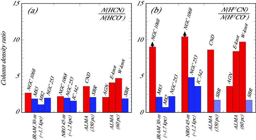
Figure 19: Column density ratios of (a) $N$(HCN)/$N$(HCO⁺) and (b) $N$(H¹³CN)/$N$(H¹³CO⁺). The values with the IRAM 30-m telescope and the NRO 45-m telescope are taken from Aladro et al. (2015) and Nakajima et al. (2018), respectively. Red and blue columns represent the values in the CND (or AGN) of NGC 1068 and in the SBR of NGC 1068 or starburst galaxies, respectively. Light blue columns in (b) represent the upper-limit of both the numerator and denominator of a fraction because both H¹³CN and H¹³CO⁺ are not detected.

4.4 Column density ratios in the AGN

An enhancement of the HCN ($J$ = 1–0) intensity relative to HCO⁺ ($J$ = 1–0) ($I$(HCN)/$I$(HCO⁺)) toward the Seyfert nuclei compared with the nuclear starburst galaxies at a few 100 pc scales has been proposed in previous studies (e.g., Kohno et al., 2001; Kohno, 2005), and this trend was also confirmed in NGC 1068. Kohno et al. (2008) reported that $R_{{\rm HCN/HCO^{+}}}$ toward the CND and the SBR in NGC 1068 are 2.1 and approximately unity, respectively, as measured with the Nobeyama Millimeter Array (NMA). Therefore, $I$(HCN)/$I$(HCO⁺) may be a useful discriminator for the galactic power source between AGN and starburst activity. In addition, this trend with higher transition HCN ($J$ = 4–3) and HCO⁺ ($J$ = 4–3) lines is clearer than that of the fundamental transition lines (Izumi et al., 2016). However, the column density ratio $N$(HCN)/$N$(HCO⁺) in NGC 1068 and that in typical starburst galaxies are almost the same value with single-dish telescopes (Aladro et al., 2015; Nakajima et al., 2018). These studies reported that the values of $N$(HCN)/$N$(HCO⁺) do not exhibit a clear trend corresponding to the type of galactic activity. The authors of previous studies have proposed that probable reasons for the lack of a trend are the low angular resolution and the effect of the optical depth. Moreover, Nakajima et al. (2018) proposed that the ¹³C isotopic species ratio (i.e., $N$(H¹³CN)/$N$(H¹³CO⁺)) with optically thin lines, is significantly enhanced in NGC 1068 and in typical starburst galaxies with values of $>$10.4 and $\sim$4–5, respectively, and could be more useful for differentiation.

In this study, we estimate the column density ratios with the 350 and 60 pc scales, as shown in Figure 19. In $N$(HCN)/$N$(HCO⁺) estimated at 350 pc, we determined that the ratios in the CND and SBR are 3.6 and 2.1, respectively. The value in the CND is twice as large as that in the SBR and is much different from that obtained by single-dish telescopes (Figure 19(a)). Therefore, a high spatial resolution is important to determine the difference in these ratios among different galaxies. In addition, we found that the ratios in the E- and W-knots are higher than those in the AGN position compared with those in the SBR with a 60 pc scale. This indicates that the ring structure surrounding the AGN at $\sim$200 pc, rather than the gas component at the AGN position, further contributes to the enhancement of $N$(HCN)/$N$(HCO⁺) in the AGNs. These features are clearer in the ratio using ¹³C isotopic species (Figure 19(b)).

According to the model calculation, a high-temperature reaction ${\rm CN+H_{2}\longrightarrow HCN+H}$ efficiently converts CN into HCN, reducing the fractional abundance of CN at elevated temperatures and increasing that of HCN in hot environments (Harada et al., 2010). Therefore, the enhancements of HCN and H¹³CN in the CND may be due to the high-temperature environment. Izumi et al. (2013) claimed that the reason for the HCN increase is mechanical heating due to the shock by the AGN jet. In fact, the E-knot is likely to be heavily shocked based on observations of the shock tracers SiO, HNCO, CH₃OH, and chemical model calculations (Garcia-Burillo et al., 2010; Kelly et al., 2017). We also confirmed that the distribution of H¹³CN in the CND is strongly correlated with the emission of SiO, which is well-known as a strong shock tracer, with additional ALMA observations (A. Taniguchi et al. in prep.).

$N$(CN)/$N$(HCN) is expected to have a large value that lies between 40 (at $n\sim$10⁶ cm^-3) and over 1000 (at $n\sim$10⁴ cm^-3) in an XDR model (Meijerink et al., 2007). The density in the CND was estimated to be 10⁵–10⁶ cm^-2 toward the CND and AGN positions (Scourfield et al., 2020). In contrast, the estimated value in our study is approximately 15 in the CND, which is smaller (1/3–1/5) than that in the SBR. Therefore, the high-temperature environment resulting from mechanical heating in the CND is more effective than the expected strong X-ray and/or cosmic ray irradiation from the AGN based on the footprint of molecular compositions.

However, we reported a significant enhancement of $N$(CN) in the CND compared to that in the SBR based on another ALMA observation of the higher transition line $N$ = 3–2 (Nakajima et al., 2015). In this study, higher transition lines are not used for analysis because CN emission lines are located in the band edge of the spectrometer, and the detection is only partial. For a more accurate estimation of the physical properties of these molecules, it is necessary to obtain information on multiple transitions.

5 Conclusions

In this paper, we present an imaging molecular line survey in the 3-mm band (85–114 GHz) toward one of the nearest galaxies with an AGN, NGC 1068, based on observations taken with ALMA. This is the first line survey with high resolution that can resolve the internal structure of the circumnuclear disk (CND) at the nucleus in an AGN host of a nearby galaxy. The results and discussion are summarized as follows.

1. A total of 23 molecular gas distributions are obtained covering the entire structure of the central region, which consists of the CND and starburst ring (SBR), with 60 and/or 350 pc resolution. We detected a ²⁹SiO line for the first time toward NGC 1068. Moreover, non-detection lines in the previous line survey with the NRO 45-m telescope, H¹³CO⁺ and CH₃CN ($J_{K}$ = 5_K–4_K), are clearly detected and imaged using the ALMA.

2. The strong emissions of H¹³CN, H¹³CO⁺, SiO, HC₃N, CH₃CN, SO, and ¹³CN are concentrated in the CND, while weak emission is either seen or not seen in the SBR with 350 pc scale observations. Takano et al. (2014) already reported this feature for HC₃N, CH₃CN, SO, and ¹³CN, and we newly confirmed that other molecules have similar characteristics. The enhancement of these molecules in the CND may be a result of the effect of the AGN. In addition, CH₃OH and HNCO ($J_{Ka,Kc}$ = 5_0,5–4_0,4) have a characteristic distribution in the SBR. Their peak positions are clearly different from that of ¹²CO. Such a feature for CH₃OH was reported by Tosaki et al. (2017), and we newly found that HNCO has a similar trend. These molecules may reflect dynamic effects, such as cloud-cloud collisions and/or galaxy dynamics because they are known as shock tracers.

3. The following molecules have significantly strong emissions from the E-knot relative to the W-knot: c-C₃H₂, ²⁹SiO, H¹³CO⁺, CH₃CN, N₂H⁺, C³⁴S, SO, and ¹³CO with 60 pc scale observations. Although there are no molecular lines of stronger emission from the W-knot than that from the E-knot, there are various peak intensity positions in the W-knot for molecules.

4. In the fractional abundances relative to CS in the CND, AGN position, and SBR, the abundant molecules in the CND with the 350 pc scale and in the AGN with the 60 pc scale are almost similar in the two resolutions. H¹³CN, SiO, HCN, and H¹³CO⁺ show enhancements in the whole of the CND as well as the AGN position. These HCN, H¹³CN, H¹³CO⁺, and ¹³CO trends were already reported using single-dish telescopes compared with the typical starburst galaxies (Aladro et al., 2013; Nakajima et al., 2018), and ALMA observations (Butterworth et al. 2022). However, the enhancement of SiO in the CND relative to the SBR is newly found thanks to high-resolution imaging with ALMA. However, ¹³CO shows an enhancement in the SBR compared to that in the CND and AGN.

5. Except for the CO isotopologue, the abundance of almost all molecules with ALMA (350 pc scale) are consistent with those with the NRO 45-m telescope ($\sim$1.2 kpc). SiO and H¹³CN are significantly enhanced, and HNC, N₂H⁺, C₂H, HCN, c-C₃H₂, HNCO, and HC₃N are also slightly enhanced compared with those with 1.2 kpc. This may be because of the effect of AGN on surrounding molecular gas depending on the observational scale.

6. We estimate column density ratios $N$(HCN)/$N$(HCO⁺) and $N$(H¹³CN)/$N$(H¹³CO⁺) with 350 and 60 pc scales. $N$(HCN)/$N$(HCO⁺) in the CND is twice as large as that in the SBR, and it is significantly different from that obtained by the single-dish telescopes. Therefore, high spatial resolution is important to determine the difference in these ratios among different galaxies. This feature is more clearly observed in the ratio using ¹³C isotopic species.

7. Based on the column density ratios of $N$(HCN)/$N$(HCO⁺)and $N$(CN)/$N$(HCN), the enhancements of HCN in the CND are possibly due to the high-temperature environment, which was claimed by Harada et al. (2010) and Izumi et al. (2013). The expected strong X-ray and/or cosmic ray irradiation from the AGN have relatively less impact on the molecular abundance in the CND than mechanical feedback.

Appendix A Rotation diagram

The rotational temperatures ($T_{\rm rot}$) were calculated using the rotation diagram approach (Figure 20) under the assumption of local thermodynamic equilibrium (LTE), that all lines are optically thin, and that a single excitation temperature characterizes all transitions (e.g., Goldsmith & Langer (1999)). In this study, multiple transition lines in the 3-mm band were detected in three molecules (HNCO (4_0,4–3_0,3 and 5_0,5–4_0,4); HC₃N (10–9, 11–10, and 12–11); and CH₃CN (5_K–4_K and 6_K–5_K). For CH₃CN, we apply a method of separating blended lines based on Martín et al. (2006) because the transitions of different K ladders are blended. For CS, C¹⁸O, and ¹³CO, we used the data in the 3-mm and 0.8-mm band (Nakajima et al., 2015) to plot the rotation diagrams. Note that the errors of HNCO and HC₃N (11–10) in the SBR are too large (S/N less than 3$\sigma$); thus, we did not use the calculated $T_{\rm rot}$ of this molecule for the estimation of $N_{\rm mol}$.

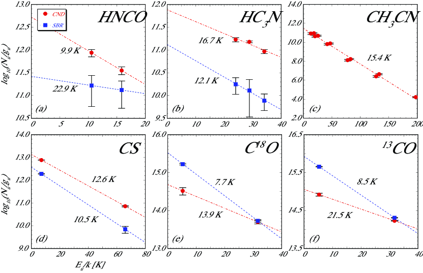
Figure 20: The rotational diagram of each molecule (a) HNCO, (b) HC₃N, (c) CH₃CN, (d) CS, (e) C¹⁸O, and (f) ¹³CO in the CND (circle symbols) and the SBR (square symbols). The calculated rotational temperatures are shown beside a fitting line. The error bars are based on the $\pm$1$\sigma$ noise level of integrated flux.

Appendix B Column densities of molecules

The column densities are calculated using the following equation, which is described in detail in Turner (1991):

$${\rm log}\left(\frac{N_{\rm mol}}{Z}\right)={\rm log}\frac{8{\pi}k{\nu}^{2}}{hc^{3}A_{ul}g_{u}g_{I}g_{K}}W+\frac{E_{u}}{k}\frac{{\rm log}\,e}{T_{\rm rot}},$$ (B1)

where $N_{\rm mol}$ is the column density, $Z$ is the partition function, $\nu$ is the frequency, $A_{ul}$ is the Einstein A-coefficient, $g_{u}$ is the rotational degeneracy of the upper state (2$J_{u}$ + 1), $g_{I}$ and $g_{K}$ are the reduced nuclear spin degeneracy and $K$-level degeneracy, respectively, and $E_{u}$ is the energy of the upper state of the transition. In this study, we obtained the value of the partition function from the Cologne Database for Molecular Spectroscopy (CDMS; Müller et al. (2005)). However, note that the spin degeneracy $g_{I}$ of 3 for the ¹⁴N nucleus is included in the partition functions of HCN, H¹³CN, N₂H⁺, CN, and ¹³CN. In addition, those of radicals in the 2$\Sigma$ electronic state, C₂H, CN, and ¹³CN, are included in the spin doublet of 2. It is necessary to consider the included degeneracies when calculating $N_{\rm mol}$ using the partition function in the database. In particular, because the degeneracies of $g_{I}$ and/or $g_{K}$ for cyclic-C₃H₂, CH₃OH and CH₃CN are complicated, we do not use the partition function in the CDMS. Details pertaining to the calculations for these molecules were explained in our previous paper (Nakajima et al., 2018).

References

- Aladro et al. (2013) Aladro, R., Viti, S., Bayet, E., et al. 2013, A&A, 549, A39
- Aladro et al. (2015) Aladro, R., Martín, S., Riquelme, D., et al. 2015, A&A, 579, A101
- Bayet et al. (2009) Bayet, E., Aladro, R., Martín, S, Viti, S. & Martín-Pintado, J. 2015, ApJ, 707, 126
- Butterworth et al. (2022) Butterworth, J., Holdship, J., Viti, S, & García-Burillo, S. 2022, A&A, 667, A131
- Chin et al. (1999) Chin, Y.-N., Henkel, C., Langer, N., & Mauersberger, R. 1999, ApJ, 512, L143
- Costagliola et al. (2015) Costagliola, F., Sakamoto, K., Muller, S., et al. 2015, A&A, 582, A91
- Das et al. (2006) Das, V., Crenshaw, D. M., Kraemer, S. B., & Deo, R. P. 2006, AJ, 132, 620
- Davis et al. (2013) Davis, T. A., Heiderman, A., Evans II, N. J., & Iono, D. 2013, MNRAS, 436, 570
- Gallimore et al. (1996) Gallimore, J. F., Baum, S. A., O’Dea, C. P., & Pedlar, A. 1996, ApJ, 458, 136
- Gallimore et al. (2004) Gallimore, J. F., Baum, S. A., & O’Dea, C. P. 2004, ApJ, 613, 794
- Garcia-Burillo et al. (2010) García-Burillo, S., Usero, A., Fuente, A., et al. 2010, A&A, 519, A2
- Garcia-Burillo et al. (2014) García-Burillo, S., Combes, F., Usero, A., et al. 2014, A&A, 567, A125
- Garcia-Burillo et al. (2016) García-Burillo, S., Combes, F., Ramos Almeida, C., et al. 2016, ApJ, 823, L12
- Garcia-Burillo et al. (2017) García-Burillo, S., Viti, S., Combes, F., et al. 2017, A&A, 608, A56
- Goldsmith & Langer (1999) Goldsmith, P. F., & Langer, W. D. 1999, ApJ, 517, 209
- Harada et al. (2010) Harada, N., Herbst, E., & Wakelam, V. 2010, ApJ, 721, 1570
- Harada et al. (2018) Harada, N., Sakamoto, K., Martín, S., et al. 2018, ApJ, 855, 49
- Helfer et al. (1995) Helfer, T. T., & Blitz, L. 1995, ApJ, 450, 90
- Holdship et al. (2017) Holdship, J, Viti, S., Jiménez-Serra, I., Makrymallis, A., & Priestley, F. 2017, AJ, 154, 38
- Huang et al. (2022) Huang, K. -Y., Viti, S., Holdship, J., et al. 2022, A&A, 666, A102
- Imanishi et al. (2018) Imanishi, M., Nakanishi, K., Izumi, T., & Wada, K. 2018, ApJ, 853, L25
- Imanishi et al. (2020) Imanishi, M. Nguyen, D. D., Wada, K., et al., 2020, ApJ, 902, 99
- Izumi et al. (2013) Izumi, T. Kohno, K., Martín, S., et al., 2013, PASJ, 65, 100
- Izumi et al. (2016) Izumi, T., Kohno, K., Aalto, S., et al. 2016, ApJ, 818, 42
- Jansen et al. (1995) Jansen, D. J., van Dishoeck, E. F., Black, J. H., Spaans, M., & Sosin, C. 1995, A&A, 302, 223
- Kaneko et al. (1992) Kaneko, N., Morita, K., Fukui, Y., et al. 1992, PASJ, 44, 341
- Kelly et al. (2017) Kelly, G., Viti, S., García-Burillo, S., et al. 2017, A&A, 597, A11
- Kohno et al. (2001) Kohno, K., Matsushita, S., Vila-Vilaró, B., et al. 2001, in ASP Conf. Ser. 249, The Central Kiloparsec of Starbursts and AGN: The La Palma Connection, ed. J. H. Knapen et al. (San Francisco, CA: ASP), 672
- Kohno (2005) Kohno, K. 2005, in AIP Conf. Ser., 783, The Evolution of Starbursts: The 331stWilhelm and Else Heraeus Seminar, ed. S. Hüttemeister et al. (New York: AIP), 203
- Kohno et al. (2008) Kohno, K., Nakanishi, K., Tosaki, T., et al. 2008, Ap&SS, 313, 279
- Lilley & Palmer (1968) Lilley, A. E., & Palmer, P. 1968, ApJS, 16, 143
- Lovas (2004) Lovas, F. J. 2004, J. Phys. Chem. Ref. Data, 33, 177
- Maloney et al. (1996) Maloney, P. R., Hollenbach, D. J. & Tielens, A. G. G. M. 1996, ApJ, 466, 561
- Martín et al. (2006) Martín, S., Mauersberger, R., Martín-Pintado, J., Henkel, C., & García-Burillo, S. 2006, ApJS, 164, 450
- Martín et al. (2009) Martín, S., Martín-Pintado, J., & Mauersberger, R. 2009, ApJ, 694, 610
- Martín et al. (2015) Martín, S., Kohno, K., Izumi, T., et al. 2015, A&A, 573, A116
- Martín et al. (2021) Martín, S., Mangum, J. G., Harada, N., et al. 2021, A&A, 656, A46
- McMullin et al. (2007) McMullin, J. P., Waters, B., Schiebel, D., Young, W., & Golap, K. 2007, Astronomical Data Analysis Software and Systems XVI (ASP Conf. Ser. 376), ed. R. A. Shaw, F. Hill, & D. J. Bell (San Francisco, CA: ASP), 127
- Meijerink & Spaans (2005) Meijerink, R., & Spaans, M. 2005, A&A, 436, 397
- Meijerink et al. (2007) Meijerink, R., Spaans, M., & Israel, F. P. 2007, A&A, 461, 793
- Muxlow et al. (1996) Muxlow, T. W. B., Pedlar, A., Holloway, A. J., Gallimore, J. F., & Antonucci, R. R. J. 1996, MNRAS, 278, 854
- Müller et al. (2005) Müller, H. S. P., Schlöder, F., Stuzki, J., & Winnewisser, G. 2005, J. Mol. Struct., 742, 215
- Nakajima et al. (2015) Nakajima, T., Takano, S., Kohno, K., et al. 2015, PASJ, 67, 8
- Nakajima et al. (2018) Nakajima, T., Takano, S., Kohno, K., Harada, N., & Herbst, E. 2018, PASJ, 70, 7
- Nishimura et al. (2016) Nishimura, Y., Shimonishi, T., Watanabe, Y., et al. 2016, ApJ, 829, 94
- Papadopoulos et al. (1996) Papadpoulos, P. P., Seaquist, E. R., & Scoville, N. Z. 1996, ApJ, 465, 173
- Planesas et al. (1991) Planesas, P., Scoville, N., & Myers, S. T. 1991, ApJ, 369, 364
- Qiu et al. (2018) Qiu, J., Wang, J., Shi, Y., et al. 2018, A&A, 613, A3
- Qiu et al. (2020) Qiu, J., Zhang, J., Zhang, Y., Jia, L., & Tang, X., 2020, A&A, 634, A125
- Saito et al. (2022a) Saito, T., Takano, S., Harada, N., et al. 2022a, ApJ, 927, L32
- Saito et al. (2022b) Saito, T., Takano, S., Harada, N., et al. 2022b, ApJ, 935, 155
- Sánchez-García et al. (2022) Sánchez-García, M., García-Burillo, S., Pereira-Santaella, M., et al. 2022, A&A, 660, A83
- Schinnerer et al. (2000) Schinnerer, E., Eckart, A., Tacconi, L. J., Genzel, R., & Downes, D. 2000, ApJ, 533, 850
- Scourfield et al. (2020) Scourfield, M., Viti, S., García-Burillo, S., et al. 2020, MNRAS, 496, 5308
- Skatrud et al. (1983) Skatrud, D. D., De Lucia, F. C., Blake, G. A., & Sastry, K. V. L. N. 1983, Journal of Molecular Spectroscopy, 99, 35
- Tacconi et al. (1994) Tacconi, L. J., Genzel, R., Blietz, M., et al. 1994, ApJ, 426, L77
- Tacconi et al. (1997) Tacconi, L. J., Gallimore, J. F., Genzel, R., Schinnerrer, E., & Downes, D. 1997, Ap&SS, 248, 59
- Takano et al. (2014) Takano, S., Nakajima, T., Kohno, K., et al. 2014, PASJ, 66, 75
- Takano et al. (2019) Takano, S., Nakajima, T., & Kohno, K., 2019, PASJ, 71, S20
- Tang et al. (2019) Tang, X. D., Henkel, C., Menten, K. M., et al. 2019, A&A, 629, A6
- Telesco & Decher (1988) Telesco, C. M., & Decher, R. 1988, ApJ, 334, 573
- Tosaki et al. (2017) Tosaki, T., Kohno, K., Harada, N., et al. 2017, PASJ, 69, 18
- Tsai et al. (2012) Tsai, M., Hwang, C.-Y., Matsushita, S, Baker, A. J., & Espada, D. 2012, ApJ, 746, 129
- Tully & Fisher (1988) Tully, R. B., & Fisher, J. R. 1988, Catalog of Nearby Galaxies, Cambridge University Press
- Turner (1991) Turner, B. E. 1991, ApJS, 76, 617
- van der Tak et al. (2007) van der Tak, F. F. S., Black, J. H., Schöier, F. L., Jansen, D. J., & van Dishoeck, E. F. 2007, A&A, 468, 627
- Viti et al. (2014) Viti, S., García-Burillo, S., Fuente, A., et al. 2014, A&A, 570, A28
- Wang et al. (2014) Wang, J., Zhang, Z.-Y., Qiu, J., et al. 2014, ApJ, 796, 57
- Watanabe et al. (2019) Watanabe, Y., Nishimura, Y., Sorai, K., et al. 2019, ApJS, 242, 26