Absorbing Phase Transitions
in Artificial Deep Neural Networks

Abstract

Theoretical understanding of the behavior of infinitely-wide neural networks has been rapidly developed for various architectures due to the celebrated mean-field theory. However, there is a lack of a clear, intuitive framework for extending our understanding to finite networks that are of more practical and realistic importance. In the present contribution, we demonstrate that the behavior of properly initialized neural networks can be understood in terms of universal critical phenomena in absorbing phase transitions. More specifically, we study the order-to-chaos transition in the fully-connected feedforward neural networks and the convolutional ones to show that (i) there is a well-defined transition from the ordered state to the chaotics state even for the finite networks, and (ii) difference in architecture is reflected in that of the universality class of the transition. Remarkably, the finite-size scaling can also be successfully applied, indicating that intuitive phenomenological argument could lead us to semi-quantitative description of the signal propagation dynamics.

1 Introduction

The 21st century has witnessed the tremendous success of deep learning applications. Properly trained deep neural networks have successfully demonstrated performance comparable with, or even superior to, that of human experts in various tasks, a few remarkable examples being the game of Go [1], image synthesis [2], and natural language processing [3]. Boosted by an exciting discovery of the so-called neural network scaling laws [4, 5], the frenetic pace in improving neural network performance is likely to persist, and hence it may be safe to say that deep learning technologies will constitute indispensable building blocks of the next-generation human society.

Despite the fact that practically deep learning models can achieve such impressive performances, theoretically their behaviors are not yet fully understood. Deep neural networks are usually heavily over-parametrized, with the number of parameters in state-of-the-art neural networks growing exponentially over time [6]. From an energetic viewpoint, the state-of-the-art deep learning models consume a lot of energy, as the number of parameters is correlated to the amount of energy needed to perform an inference. In contrast, human brains seem to be good at learning and generalizing in an energetically efficient manner, even though strictly speaking they are generally not at doing arithmetic operations. This suggests that placing and comparing artificial neural networks in a broader context of biological neural networks on an equal footing, at least from a functional perspective, is promising for developing their understanding.

The notion of criticality is the key to linking biological and artificial neural networks. Systems at a particular condition (e.g. at the critical point of second-order phase transitions) exhibit anomalous behavior, referred to as critical phenomena. They are universal in the sense that microscopically diverse systems can be described by a single mathematical model as long as the essential properties remain unchanged.

The critical phenomena of particular interest in neuroscience are those of absorbing phase transitions [7, 8]: transitions to a state from which a system cannot escape (hereafter referred to as “an absorbing state”). Besides the obvious analogy with brains without any neuronal activity (i.e. death), absorbing phase transitions are considered to be one of the essential ingredients for self-organized criticality [9], by which the systems can be automatically tuned to the critical point. Recent theoretical and experimental studies support the view that the brains may operate near the critical point (albeit in a slightly nuanced manner), and the universal scaling law in the critical phenomena of absorbing phase transition has been attracting considerable interest among the community; interested readers are referred to, for example, the recent review by Girardi-Schappo [10].

As a matter of fact, the deep learning research community is also familiar (albeit implicitly) with the notion of criticality. In theoretical studies on deep neural networks, the concept of the edge of chaos has played a considerable role. While the discovery of chaos in random neural networks dates back to (at least) as early as the late 1980s [11], the concept has attracted recent interest among the community when Poole et al. theoretically demonstrated that infinitely-wide deep neural networks also exhibit the order-to-chaos transition [12]. Remarkably, at the onset of chaos, trainable depth of the networks is suggested to diverge [13], which is reminiscent of the divergence of the correlation length at the critical point of second-order phase transitions at equilibrium. Furthermore, recent work has successfully applied the renormalization group method to classify the order-to-chaos transitions in the fully-connected feedforward neural networks for various activation functions into a small number of universality classes [14].

Nevertheless, we argue that the notion of criticality has not been fully exploited in studies of artificial deep neural networks. As also discussed by Hesse and Gross [15], bottom-up approaches (in which one derives macroscopic properties from microscopic theories) and top-down ones (in which one starts from phenomenological observations or some heuristics to deduce macroscopic properties) are complementary to each other for studying complicated systems. Numerous works, including those cited in the previous paragraph, have successfully adopted one of the bottom-up approaches for a specific architecture and/or an activation function. However, the situation with regard to the top-down approaches is less satisfactory. Since the universality of the critical phenomena enables the classification of the systems into a reduced number of universality classes based on their fundamental properties, taking full advantage of it would lead us to intuitive and yet powerful understanding of the behavior of deep neural networks across different architectures.

Given all these observations, the purpose of the present work is to demonstrate that the notion of absorbing phase transition is a promising tool for theoretical understanding of the deep neural networks. First, we establish an analogy between the aforementioned order-to-chaos transition and an absorbing phase transition by studying the linear stability of the ordered state. In the framework of the mean-field theory of signal propagation in deep neural networks [12], the critical point is characterized by loss of linear stability of the fixed point corresponding to the ordered phase. We extend the analysis to the networks of finite width, and we directly see that the transition to chaos in artificial deep neural networks is an emergent property of the networks which requires the participation of sufficiently many neurons (and thus more appropriately seen as a phase transition, rather than a mere bifurcation in dynamical systems).

Next, we show that the order-to-chaos transitions in initialized artificial deep neural networks exhibit the universal scaling laws of absorbing phase transition. Actually it is fairly straightforward to find the scaling exponents associated with the transition in the framework of the mean-field theory (or equivalently in the infinitely-wide networks) for the fully-connected feedforward neural networks [13], but it is not clear how we can extend the analysis into the networks of finite width or a different architecture. Our empirical study reveals that the idea of the universal scaling can still be successfully applied to such cases. We also provide an intuitive way to understand the resulting universality class for each architecture, based on a phenomenological theory. Remarkably, the finite-size scaling can also be successfully applied, indicating that intuitive phenomenological argument could lead us to semi-quantitative description of the signal propagation dynamics in the finite networks.

To summarize, we believe that the this work places the order-to-chaos transition in the initialized artificial deep neural networks in the broader context of absorbing phase transitions, and serves as the first step toward the systematic comparison between natural/biological and artificial neural networks.

2 Preliminaries

In this work, we illustrate our view with the following deep neural networks:

• FC: A fully-connected feedforward neural network of width $n$ and depth $L$. We assume the same width for all the hidden layers, although the size $n_{0}$ of the input needs not be equal to $n$. The weight matrices $W^{(l)}$ $(l=1,2,\cdots,L)$ and bias vectors $\boldsymbol{b}^{(l)}$ are initialized according to normal distribution, respectively $\mathcal{N}(0,\sigma_{w}^{2}/n)$ and $\mathcal{N}(0,\sigma_{b}^{2})$.

• Conv: A vanilla $d$-dimensional convolutional neural network (having $c$ channels) of width $n$ and depth $L$, although we mostly deal with the case $d=1$. The similar assumption as FC is also applicable for Conv. The convolutional filters $w^{(l;j,m)}$ of width $k$ (for each dimension) and bias vectors $\boldsymbol{b}^{(l;j)}$ are initialized according respectively to $\mathcal{N}(0,\sigma_{w}^{2}/(ck^{d}))$ and $\mathcal{N}(0,\sigma_{w}^{2}/(ck^{d}))$. The so-called circular padding is applied.

Formally, the recurrence relations for the preactivation ($\boldsymbol{z}^{(l)}$ for FC and $\boldsymbol{z}^{(l;\alpha)}$ for Conv) are respectively written as follows:

$$z_{i}^{(l+1)}=\sum_{j}W_{ij}^{(l+1)}h(z^{(l)}_{j})+b_{i}^{(l+1)},$$ (1)

$$z_{i}^{(l+1;\alpha)}=\sum_{\begin{subarray}{c}j\in ker,\\ m\in chn\end{subarray}}w^{(l+1;\alpha,m)}_{j+\frac{k+1}{2}}h(z_{i+j}^{(l;m)})+b_{i}^{(l+1;\alpha)},$$ (2)

where $ker=\{-(k-1)/2,\cdots,-1,0,1,\cdots,(k-1)/2\}$, $chn=\{1,2,\cdots,c\}$, and the subscripts for $z$ larger than $n$ is understood as the remainder when divided by $n$ whereas smaller than $1$ as the addition to $n$ (due to the circular padding). The activation function is assumed to be $h(x)=\tanh x$ unless otherwise stated, but we expect essentially same results to hold within a fairly large class of functions.

These initialized neural networks are known to exhibit order-to-chaos transition in the limit of infinitely wide network (for FC [12]) or infinitely many channels (for Conv [17]), as depicted in Fig. 1(a). Deep networks return almost same output for any inputs in the ordered phase, whereas correlation between similar inputs is lost in the chaotic phase. In either case, the deep networks “forget” what they were given, which is very likely to be disadvantageous for machine learning tasks. Presumably this is the central reason why the phase boundary, also known as the edge of chaos, has attracted considerable interest in the literature. As a matter of fact, recent studies have theoretically demonstrated that initialization of the network (in particular at the edge of chaos) is linked to practically important issues in deep learning: the problem of vanishing or exploding gradients [13], the dilemma between trainability and generalizability [18], to name only a few examples.

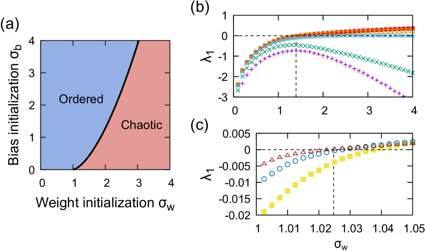
Figure 1: Absorbing phase transitions in deep neural networks. (a) Phase diagram of signal propagation in FC and Conv (see text for their formal definition). The solid curve indicates the phase boundary as derived from their respective mean-field theory [12, 17], identical with each other. (b) The maximum generalized Lyapunov exponent $\lambda_{1}$ (see Eq. (3)) in FC as a function of the weight initialization $\sigma_{w}$, numerically calculated for various width $n$ (1 (purple), 2 (green), 9 (light blue), 20 (orange) and 50 (red)). (c) Similar with (b), but now with Conv for various number of channels $c$ (from 5 (yellow) to 50 (brown)). The width $n,k$ of the network and the convolutional filters are respectively fixed to 50 and 3. The standard deviation $\sigma_{b}$ for the bias vectors is fixed to be 0.3 (for FC) and $\sqrt{20}\times 10^{-3}$ (for Conv).

A clarification comment is in order before we proceed: the two technical terms, namely the ordered state and the ordered phase are not to be confused with each other. Hereafter, the former technical term refers to the state where the two preactivations $\boldsymbol{z}_{1}^{(l)},\boldsymbol{z}_{2}^{(l)}$ corresponding to generally different inputs $\boldsymbol{x}_{1},\boldsymbol{x}_{2}$ are identical, whereas the latter to the region in the phase space $(\sigma_{w},\sigma_{b})$ where $\boldsymbol{z}_{1}$ and $\boldsymbol{z}_{2}$ almost surely become arbitrarily close to each other in the infinitely deep limit. For example, even if the combination of the hyperparameters $(\sigma_{w},\sigma_{b})$ are not in the ordered phase, it is possible that a pair of preactivations $\boldsymbol{z}_{1},\boldsymbol{z}_{2}$ reaches to the ordered state, depending on the inputs $\boldsymbol{x}_{1},\boldsymbol{x}_{2}$ and specific realizations of the weights and biases.

3 Absorbing property of the ordered state

Now let us establish an analogy between the ordered state and an absorbing state. Clearly, the ordered state is a fixed point of the signal propagation dynamics for any $\sigma_{w}$ once the weight matrices and the bias vectors are initialized. It is also clear, however, that the ordered state is almost never achieved accidentally: That is, if $\boldsymbol{z}_{1}^{(l)}\neq\boldsymbol{z}_{2}^{(l)}$ for some $l$, the probability that $\boldsymbol{z}^{(l+1)}_{1}=\boldsymbol{z}_{2}^{(l+1)}$ is zero for that $l$. Hence a more relevant question is whether the ordered state is stable against infinitesimal disturbance, at least for some $\sigma_{w}$.

To address the issue of the linear stability of the ordered state, we study the maximum Lyapunov exponent for the front propagation dynamics (1), (2) (we only display the definition for FC for convenience; extending it to Conv is straightforward):

$$\lambda_{1}:=\lim_{l\rightarrow\infty}\frac{1}{l}\log\frac{\|J^{(l)}(\boldsymbol{z}^{(l)})\cdots J^{(1)}(\boldsymbol{z}^{(1)})\boldsymbol{u}_{0}\|}{\|\boldsymbol{u}_{0}\|},$$ (3)

where $\boldsymbol{u}_{0}\in\mathbb{R}^{n}$ is an arbitrary nonzero vector and $J^{(l)}$ is the layer-wise input-output Jacobian

$$J^{(l)}(\boldsymbol{z})=\left(\begin{array}[]{ccc}J_{11}^{(l)}(\boldsymbol{z})&\cdots&J_{1n}^{(l)}(\boldsymbol{z})\\ \vdots&\ddots&\vdots\\ J_{n1}^{(l)}(\boldsymbol{z})&\cdots&J_{nn}^{(l)}(\boldsymbol{z})\\ \end{array}\right)\quad\mathrm{with}\quad J_{ij}^{(l)}(\boldsymbol{z}):=W_{ij}^{(l)}h^{\prime}(z_{j}).$$ (4)

By doing so we can directly see how the notion of the order-to-chaos transition emerges as a many-body effect in the neural networks; see the numerical results in Fig. 1(b). In the case where the hidden layer consists of only a small number $n$ of neurons (say $n\lesssim 10$ for FC), the maximum Lyapunov exponent $\lambda_{1}$ as a function of the weight initialization $\sigma_{w}$ is negative in the entire domain, which suggests that the ordered state is always stable against infinitesimal discrepancy. However, $\lambda_{1}$ increases as $n$ becomes larger, and eventually, $\lambda_{1}$ changes its sign at some $\sigma_{w}$ for large $n$, indicating loss of the linear stability. Naturally, the position of the onset of the linear instability is very close to that of the critical point predicted from the mean-field theory [12] when $n$ is large, and is expected to coincide in the limit of $n\rightarrow\infty$.

Thus, the maximum Lyapunov exponent $\lambda_{1}$ successfully captures the well-defined transition from the ordered phase to the chaotic phase even for finite networks. In the ordered phase, once a pair of preactivations $(\boldsymbol{z}_{1},\boldsymbol{z}_{2})$ reaches reasonably close to the ordered state, it is hard to escape from it. Meanwhile, in the chaotic phase, a pair of preactivations are allowed to get away from the vicinity of the ordered state, although the ordered state itself is still absorbing. This scenario, a transition from a non-fluctuating absorbing phase to a fluctuating active phase, is highly reminiscent of an absorbing phase transition in statistical mechanics.

The similar scenario also holds for Conv, but the qualitative difference from FC in the behavior of the maximum generalized Lyapunov exponent $\lambda_{1}$ in the vicinity of the critical point calls for further discussion. In Conv with fixed width $n$, we numerically observe that $\lambda_{1}$ increases as the number $c$ of channels do so in the ordered phase, whereas it decreases in the chaotic phase. This is in sharp contrast with FC, where $\lambda_{1}$ increases as $n$ do so regardless of the phase. This tendency suggests that, in the limit of $c\rightarrow\infty$, the derivative of $\lambda_{1}$ with respect to $\sigma_{w}$ vanishes at the critical point, and therefore the characteristic depth for the transition diverges faster than the reciprocal of the deviation $|\sigma_{w}-\sigma_{w;c}|$ from the critical point. Later we will provide additional evidence that the correlation depth indeed diverges faster than $|\sigma_{w}-\sigma_{w;c}|^{-1}$.

4 Universal scaling around the order-to-chaos transition

Having seen that the order-to-chaos transition is at least conceptually analogous to absorbing phase transitions, the next step is to seek the deeper connection between these two by further quantitative characterization. One of the most common strategies for studying systems with absorbing phase transition is to examine universal scaling laws [7, 8]. Systems with a continuous transition to an absorbing phase can be characterized by power-law behavior for various quantities. For example, an order parameter (a quantity that vanishes in an absorbing phase whereas remaining positive otherwise) $\rho$ and correlation time $\xi_{\|}$ for the statistically steady state respectively exhibit power-law onset and divergence with some suitable exponents

$$\rho\sim\tau^{\beta},\quad\xi_{\|}\sim|\tau|^{-\nu_{\|}}$$ (5)

in the vicinity of the critical point, where $\tau$ denotes the deviation from the critical point (we define it to be $\tau:=\sigma_{w}-\sigma_{w;c}$ in the present work, where $\sigma_{w;c}$ is the weight initialization parameter $\sigma_{w}$ at the critical point), and $\beta,\nu_{\|}$ are the exponents associated with the power-law scaling. Moreover, the exponents, hereafter referred to as the critical exponents, are universal in the sense that they are believed to depend only on fundamental properties of the system, such as spatial dimensionality and symmetry, giving rise to the concept of the universality classes. The complexity of the underlying first-principle theory is not necessarily a problem for the universal scaling; even the transition between two topologically different turbulent states of electrohydrodynamic convection in liquid crystals, of which one cannot hope to construct the comprehensible first-principle theory, has been demonstrated to exhibit clear universal scaling laws [20, 21] with the critical exponents identical with the contact process [22], a massively simplified stochastic model for population growth. Thus, the critical exponents are expected to provide a keen insight into a priori complex systems.

Some preparations are in order before we proceed:

• In the present context, the depth $l$ of the hidden layer can be regarded as time, because the signal propagates sequentially across the layers and yet simultaneously within a layer. Hereafter, the neural-network counterpart for the correlation time will be referred to as the correlation depth.

• A natural candidate for the order parameter $\rho$ in the present context, which we will use in the following, is the Pearson correlation coefficient between preactivations for different inputs, subtracted from unity so that $\rho$ vanishes in the ordered state:

  $$\rho^{(l)}[\sigma_{w};n]:=1-\frac{\sum_{i}(z_{1;i}^{(l)}-Z_{1}^{(l)})(z_{2;i}^{(l)}-Z_{2}^{(l)})}{\sqrt{\sum_{i}(z_{1;i}^{(l)}-Z_{1}^{(l)})^{2}\sum_{i}(z_{2;i}^{(l)}-Z_{2}^{(l)})^{2}}},$$ (6)

  where $\boldsymbol{z}_{1}^{(l)},\boldsymbol{z}_{2}^{(l)}\in\mathbb{R}^{n}$ is the preactivation at the $l$th hidden layer for different inputs $\boldsymbol{x}_{1},\boldsymbol{x}_{2}$, $z_{j;i}^{(l)}$ the $i$th element of $\boldsymbol{z}_{j}^{(l)}$ and $Z_{j}^{(l)}:=\frac{1}{n}\sum_{i}z_{j;i}^{(l)}$. In the case of Conv where we have multiple channels, $\rho^{(l)}$ is obtained by first calculating the correlation coefficient (6) for each channel and then taking the average over all the channels.

• While one could measure the critical exponents directly from the Eq. (5) (although one still has to formally define the correlation depth $\xi_{\|}$), the more informative approach we employ here is to examine the dynamical scaling, where we study the scaling properties of $\rho$ as a function of the depth $l$, not only that in the infinitely-deep limit. In the framework of phenomenological scaling theory described in Appendix A, one can see that $\rho$ is expected to follow the universal scaling ansatz below (here we recall $\tau:=\sigma_{w}-\sigma_{w;c}$):

  $$\lim_{n\rightarrow\infty}\rho^{(l)}[\sigma_{w};n]\simeq l^{-\beta/\nu_{\|}}f(\tau l^{1/\nu_{\|}}).$$ (7)

Now let us demonstrate the utility of the aforementioned phenomenological scaling theory with FC, where much of the critical properties can be studied in a rigorous manner. In the case of FC, the critical exponents $\beta,\nu_{\|}$ can be analytically derived as a fairly straightforward (albeit a bit tedious) extension of the theoretical analysis by Schoenholz et al. [13]: That is, we consider infinitesimally small deviation $\delta\sigma_{w}$ from the critical point $\sigma_{w;c}$ and expand the mean-field theory [12] to track the change of the position of the fixed point and of the characteristic depth ($\xi_{c}$ in Ref. [13]) up to the first-order of $\delta\sigma_{w}$ (whereas change of the infinitesimal deviation from the fixed point with respect to depth for arbitrary $\sigma_{w}$ was studied in the preceding literature [13]). We leave the detailed derivation to Appendix B, and merely quote the final results:

$$\beta_{\mathrm{FC}}=1,\quad\nu_{\|\mathrm{FC}}=1.$$ (8)

Naturally, the above scaling exponents can be empirically validated by checking the data collapse expected from Eq. (7), as we show in Fig. 2(a).

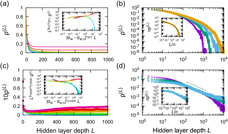
Figure 2: Universal scaling laws in the order-to-chaos transition. (a) The order parameter $\rho^{(l)}$ (see Eq. (6)) as a function of the depth $l$ of the hidden layer for various weight initialization $\sigma_{w}$ (from 1.35 (blue; ordered phase) to 1.45 (magenta; chaotic phase)) in the infinitely-wide FC, as calculated from the numerical solution of the mean-field theory [12]. The inset shows the same data rescaled according to the universal scaling ansatz (7) with critical exponents (8). (b) The order parameter $\rho^{(l)}$ at the critical point $\sigma_{w;c}\sim 1.395584$ for various width $n$ (from 50 (purple) to 400 (orange)), empirically averaged over $10^{4}$ realizations. Two orthogonal (that is, the dot product of zero) inputs of size $n_{0}=10$ were given. The inset shows the same data rescaled according to the univesal scaling ansatz (11). The black dashed curve indicates the solution of the phenomenology (10), with $\lambda=0.288,\kappa=0.686$. (c) Similar with (a), but now with the one-dimensional Conv with $n=100$ and $c=5$, empirically averaged over $10^{4}$ realizations. The two inputs $\boldsymbol{x}_{1},\boldsymbol{x}_{2}$ were set to be identical with each other, except a single element to be different by unity. The weight initialization $\sigma_{w}$ was varied from 1.41 (blue) to 1.45 (magenta). The inset shows the same data rescaled with the critical exponents of $(1+1)$-dimensional directed percolation (13). $\sigma_{w;c}=1.4335$ is chosen to find the scaling collapse. (d) Similar with (b), but now with Conv near the critical point ($\sigma_{w}=1.428$) for $n$ from 50 (purple) to 200 (light blue). The black dashed line is a guide-to-eye for $l^{-1}(=l^{-\beta_{\mathrm{FC}}/\nu_{\|\mathrm{FC}}})$. The inset shows the same data rescaled according to (11). In both FC and Conv, the standard deviation $\sigma_{b}$ for bias vectors are fixed to be 0.3.

Besides the analytical treatment, it is worthwhile to note that heuristics are also available for quickly understanding some aspects of the results. In the vicinity of the ordered state ($\rho=0$), the dynamics of the order parameter $\rho$ can be described by a linear recurrence relation at the lowest-order approximation, whose coefficient $\gamma$ is given by Jacobian of the mean-field theory at the fixed point corresponding to the ordered state. However, the linear approximation is not necessarily valid in the entire domain; in particular, one expects saturation of $\rho$ due to the bounded nature of the activation function (note also that, for the present definition (6) of the order parameter, the range of $\rho$ is bounded in the first place), which gives rise to a quadratic loss preventing $\rho$ from diverging to infinity. To sum up, one arrives at the following approximate description for the dynamics of $\rho$:

$$\frac{\mathrm{d}\rho}{\mathrm{d}l}=\gamma(\tau)\rho-\kappa\rho^{2},$$ (9)

where $\gamma(\tau)$ and $\kappa$ are phenomenological parameters (here we emphasized the dependence of $\gamma$ on the deviation $\tau$ from the critical point; the sign of $\gamma$ and $\tau$ should be the same). The above equation coincides with the mean-field theory for absorbing phase transitions [7, 8], and it admits the universal scaling ansatz (7) with the critical exponents (8). Of course, higher-order corrections are present in reality, but they do not affect the scaling properties of the networks (that is, the corrections are irrelevant in the sense of renormalization group in statistical mechanics).

A real virtue of the phenomenological scaling argument is that it provides us useful intuition even into the networks of finite width, where quantitatively tracking the deviation from the Gaussian process can be cumbersome (if not impossible [23, 24]). To illustrate this point, let us consider the finite-size scaling of FC at the critical point (corresponding to $\tau=0$ in the above heuristic argument). One can observe that the fourth-order (and other even-order) cumulants come into play in the case of finite networks, although the third-order (and other odd-order, except the first) ones vanish because the activation function is odd. In the spirit of the asymptotic expansion of the probability distribution [25], this observation indicates that the leading correction to the Gaussian process is an order of $n^{-1}$, the reciprocal of the width. Thus, together with a trivial fact that $\rho=0$ is an absorbing state also for the finite networks, we are led to the following modified phenomenology:

$$\frac{\mathrm{d}\rho}{\mathrm{d}l}=-\frac{\lambda}{n}\rho-\kappa\rho^{2},$$ (10)

which admits the finite-size scaling ansatz below:

$$\rho^{(l)}[\sigma_{w}=\sigma_{w;c};n]\simeq n^{-1}f(n^{-1}l).$$ (11)

We empirically checked whether the universal scaling ansatz (11) indeed holds for FC, and the result was affirmative, at least to a good approximation; see the data collapse in Fig. 2(b). It is interesting to note that the phenomenology (10) can be solved analytically to find

$$n\rho^{(l)}=\frac{\rho_{0}\lambda}{\rho_{0}\kappa(e^{\frac{\lambda l}{n}}-1)+(\lambda/n)e^{\frac{\lambda l}{n}}}.$$ (12)

The empirical results for $\rho^{(l)}$ after the scaling collapse can be fitted reasonably well by (12) with a suitable choice of the parameters $\rho_{0},\lambda,\kappa$. In particular, one can see that the solution (12) exhibits a crossover from the power-law decay to the exponential one at $l/n\sim 1/\lambda$, based on which one can judge whether a given deep neural network is exceedingly wide compared to its depth or vice versa. Thus the phenomenological scaling argument serves as a fast track to the recent theoretical idea that the width-to-depth ratio is a more informative quantity for describing the properties of the network than the nominal depth or width is, at least in the case of FC [14].

Next we study Conv to demonstrate that different network structure results in different universality class the network belongs to. Our empirical studies (see Fig. 2(c)) suggest that, like FC, the universal scaling ansatz (7) remains valid for Conv, although we cannot expect clear scaling collapse if $\sigma_{w}$ is too close to the critical point, due to the so-called finite-size effects. The associated critical exponents, however, are considerably different from FC (Eq. (8)); rather they are close to those of the directed percolation (DP) [26] in $(1+1)$-dimension (that is, both the preferred direction and the space perpendicular thereto is one-dimensional) [27]:

$$\beta_{\mathrm{1DDP}}\sim 0.27649,\quad\nu_{\|\mathrm{1DDP}}\sim 1.73385.$$ (13)

Again we argue that, equipped with some prior knowledge in statistical mechanics, the difference between FC and Conv can be understood quite naturally. In the case of FC, a single neuron in a hidden layer is connected to all the neurons in the one layer above. Regarding the depth as time and speaking in physics language, each neuron is effectively in a very high-dimensional space, in which case one typically expects the mean-field scaling. In contrast, the neurons in Conv interact only locally through the convolutional filters, and the mean-field picture does not necessarily apply. In this case, the robustness of the DP universality class is the key; it is conjectured by Janssen and Grassberger [28, 29] that systems exhibiting continuous phase transition into absorbing state without exceptional properties (long-range interaction, higher symmetry, etc.) belong to the DP universality class. Since the exceptional properties seem absent in Conv, it is natural to expect the DP universality, and the results in Fig. 2(c) suggest that this is indeed the case. The discussion presented here indicates that the spatial dimensionality of the network is relevant for describing the signal propagation dynamics in Conv. In passing, we have checked (though Figures are not shown) that the essentially same scenario holds true for the two-dimensional Conv ($d=2$), where the critical exponents $\beta,\nu_{\|}$ are replaced [30, 31] with

$$\beta_{\mathrm{2DDP}}\sim 0.58,\quad\nu_{\|\mathrm{2DDP}}\sim 1.29.$$ (14)

The locality of the connections for Conv induces the correlation width $\xi_{\perp}$ within a hidden layer. The correlation width $\xi_{\perp}$ for a system within the $(1+1)$-dimensional DP universality class exhibits power-law divergence with the following critical exponent $\nu_{\perp\mathrm{1DDP}}$:

$$\xi_{\perp}\sim\tau^{-\nu_{\perp\mathrm{1DDP}}}\quad\mathrm{with}\quad\nu_{\perp\mathrm{1DDP}}\sim 1.09685.$$ (15)

Importantly, the exponent $\nu_{\perp}$ for the correlation width does not coincide with the exponent $\nu_{\|}$ for the correlation depth. This fact can be seen as a caution: the most informative combination of the network width $n$ and the depth $L$ for describing the behavior of the neural networks is generally nontrivial (one might be tempted to simply use the ratio $L/n$, and indeed this works for FC, but not necessarily for other architectures). In the case where an intralayer length scale is well-defined (unlike FC), the universal scaling ansatz for the finite-size scaling in the intermediate layer $l$

$$\rho^{(l)}[\sigma_{w}=\sigma_{w;c};n]\simeq n^{-\beta/\nu_{\perp}}f(n^{-\nu_{\|}/\nu_{\perp}}l)$$ (16)

can be derived within the framework of the phenomenological scaling theory, just as we did for Eq. (7) (see also Appendix A). That is, the most informative combination of the width $n$ and the depth $L$ for describing the behavior of the critically initialized deep neural networks may be $L/n^{\nu_{\|}/\nu_{\perp}}$.

Finally, one may wonder whether the DP universality presented here for Conv with a finite number $c$ of channels is coherently connected to the $c\rightarrow\infty$ limit, where the signal propagation dynamics is reduced to the mean-field theory [17]. In the case of finite $c$, the phenomenology is similar to that in the diffusive contact process [32]. That is, we expect the existence of the depth scale $l^{*}$ below which the network effectively exhibits the mean-field scaling. Indeed, in the vicinity of the critical point $\sigma_{w;c}$, we can observe the power-law decay of the order parameter $\rho^{(l)}$ in agreement with the mean-field universality class (8) for sufficiently small $l$ (see Fig. 2(d)). Conversely, we expect the DP scaling at a depth scale larger than $l^{*}$. The depth scale $l^{*}$ at which the crossover occurs increases with $c$, and eventually diverges in the $c\rightarrow\infty$ limit, meaning that the mean-field scaling is fully recovered.

5 Discussions

In the present work, we pursued the analogy between the behavior of the classical deep neural networks and absorbing phase transitions. During the pursuit, we performed the linear stability analysis of the ordered-to-chaos transition for the neural networks of finite width or channels and uncovered the universal scaling laws in the signal propagation process in the initialized networks. In the language of absorbing phase transitions, the structural difference between FC and Conv, namely the locality of the coupling between the neurons within a hidden layer, is reflected in the universality class and thereby the value of the critical exponents. Thus we demonstrated the promising potential of heuristic argument for the semi-quantitative description of the deep neural networks.

Let us turn ourselves back to the question of similarities and differences between human brains and the artificial deep neural networks. The present work suggests that, if adequately initialized, even classical deep neural networks utilize the criticality of absorbing phase transitions, just like the brains, at the early stage of the training process. However, it is easy to see experimentally that the weights and biases cease to be at the critical point during the training unless one designs the network to be extremely wide compared to the depth. This suggests that the classical networks equipped with typical optimization schemes do not have the auto-tuning mechanisms toward the criticality. It remains to be an important question whether (and if so, how) such auto-tuning mechanisms are implemented in the state-of-the-art architectures and/or optimization schemes.

We foresee some interesting directions for future work. One of the most natural directions is to extend the present analysis to the backpropagation and to analyze the training dynamics. The neural tangent kernel (NTK) [33] has played a crucial role in the study of the training dynamics in the infinitely-wide deep neural networks, but it is repeatedly argued in the literature that the infinitely-wide limit cannot fully explain the success of deep learning [34, 35]. We are aware that some of the recent works extend the analysis beyond the infinitely-wide limit [36]. It would be interesting to see how the bottom-up approach established in the literature and the top-down one presented here can be merged into a further improved understanding of deep learning. In particular, going beyond the infinitely-many-channel limit for Conv solely by the bottom-up approaches is not very likely to be feasible due to the notorious mathematical difficulty of the directed percolation problem [37]. In this case, we believe an appropriate combination of rigorous analysis and heuristics is necessary to make progress.

Limitations.

The attempt to characterize the behavior of artificial deep neural networks in terms of absorbing phase transitions is admittedly at its infancy. The most critical limitation in our opinion is that we only dealt with the classical cases where the signals propagate across the hidden layers in a purely sequential manner. As such, extension of the present analysis to the networks of more practical use is not necessarily straightforward, although the notion of the edge of chaos is still valid in some of these cases [38, 39] and therefore one should not be too pessimistic about the feasibility. Note also that implication of the analogy on the learning dynamics has not been thoroughly investigated. Thus this is not the end of the story at all; rather it is only the beginning. Nevertheless, we hope that the this work accelerates the use of recent ideas in statistical mechanics for improving our understanding of deep learning.

Appendix A Basics of phenomenological scaling theory

The purpose of this section is to briefly recall the phenomenological scaling theory for non-equilibrium phase transitions, as the readers are not necessarily familiar with statistical mechanics. In the phenomenological scaling theory we employ throughout the paper, we postulate the following two ansatzes:

1. The behavior of systems near a critical point can be characterized by a single correlation length $\xi_{\perp}$ (if any) and a single correlation time $\xi_{\|}$. These length scales diverge at the critical point.

2. Any measurable quantities which characterize the transition (that is, vanish or diverge at the critical point) exhibit power law scaling with a suitable exponent (often called a critical exponent) as we vary the discrepancy from the critical point.

For example, let us consider a measurable quantity $\rho$ (with the critical exponent $\beta(>0)$), which depends on time $t$ and the (signed) discrepancy $\tau$ from the critical point. Then, the first ansatz states that $\rho(t,\tau)$ is a function of $t/\xi_{\|}$, parameterized by $\tau$:

$$\rho(t,\tau):=R_{\tau}(t/\xi_{\|,\tau}).$$ (17)

Thus the first ansatz introduces a one-parameter family of functions $R=\{R_{\tau}:\mathbb{R}\rightarrow\mathbb{R}|\tau\in\mathbb{R}\}$. The second ansatz is about the relationship between different members of the one-parameter family. That is, we postulate that the correlation time $\xi_{\|}$ (the critical exponent for the correlation time is conventionally denoted as $-\nu_{\|}$) and the function $R_{\tau}$ is scaled respectively by $\lambda^{-\nu_{\|}}$ and $\lambda^{\beta}$, as the discrepancy $\tau$ is multiplied by a factor $\lambda>0$:

$$\xi_{\|,\lambda\tau}=\lambda^{-\nu_{\|}}\xi_{\|,\tau},\quad R_{\lambda\tau}(x)=\lambda^{\beta}R_{\tau}(x)\ \mathrm{for}\ \forall x\in\mathbb{R}.$$ (18)

In order to demonstrate how one can obtain useful formulae from this theoretical framework, let us derive Eq. (7) in the main text. The following equality immediately follows from Eq. (18):

$$R_{\tau}(t/\xi_{\|,\tau})=\lambda^{-\beta}R_{\lambda\tau}(\lambda^{-\nu_{\|}}t/\xi_{\|,\lambda\tau}).$$ (19)

By recalling Eq. (17) and substituting $(t/T)^{1/\nu_{\|}}$ (where $T$ is an arbitrary constant having a dimension of time) into $\lambda$, we find

$$\rho(t,\tau)=(t/T)^{-\beta/\nu_{\|}}\rho(T,(t/T)^{1/\nu_{\|}}\tau).$$ (20)

The above result implies that $t^{\beta/\nu_{\|}}\rho(t,\tau)$ is a function of $\tau t^{1/\nu_{\|}}$

$$\rho(t,\tau)=t^{-\beta/\nu_{\|}}f(\tau t^{1/\nu_{\|}}),$$ (21)

which can be checked by examining a data collapse, as we have seen in Fig. 2.

If the system has a well-defined length (unlike FC), the phenomenological scaling theory can be extended to study the universal scaling properties within finite system size $L$. In this case, the first ansatz states that $\rho(t,\tau,L)$ is a function of $t/\xi_{\|}$ and $L/\xi_{\perp}$, parameterized by $\tau$:

$$\rho(t,\tau,L):=R_{\tau}(t/\xi_{\|,\tau},L/\xi_{\perp,\tau})$$ (22)

Then, by repeating the same argument as before, we arrive at the following finite-size scaling ansatz:

$$\rho(t,\tau,L)\simeq\lambda^{-\beta}g(\lambda^{-\nu_{\|}}t,\lambda\tau,\lambda^{-\nu_{\perp}}L),$$ (23)

where $-\nu_{\perp}$ is the critical exponent for the correlation length, and $g$ is a suitable scaling function.

An important point here is that the critical exponents are believed to be universal. Systems with continuous phase transitions are classified into a small number of universality classes, and systems within the same universality class share the same essential properties and the critical exponents. Hence essential mechanisms behind the transition can be deduced from measurements of the critical exponents. Interested readers are referred to the textbook by Henkel et al. [7] for further details; alternatively, a preprint of the review article by Hinrichsen [8] is freely available on arXiv.

Appendix B Derivation of the critical exponents for FC

Here we show the derivation of Eq. (8) in the main text. The starting point is the mean-field theory of the preactivations of FC by Poole et al. [12], which becomes exact in the limit of infinitely wide network [42, 43]:

$$q^{(l+1)}=\sigma_{w}^{2}\int\mathrm{d}z\frac{1}{\sqrt{2\pi}}e^{-\frac{z^{2}}{2}}h^{2}(\sqrt{q^{(l)}}z)+\sigma_{b}^{2};$$ (24)

$$c^{(l+1)}=\frac{1}{\sqrt{q_{1}^{(l)}q_{2}^{(l)}}}\left[\sigma_{w}^{2}\int\mathrm{d}z_{1}\int\mathrm{d}z_{2}\frac{1}{\sqrt{(2\pi)^{2}}}e^{-\frac{z_{1}^{2}+z_{2}^{2}}{2}}h(u_{1}^{(l)})h(u_{2}^{(l)})+\sigma_{b}^{2}\right],$$ (25)

where $q^{(l)}$ denotes the variance of the preactivation at the $l$th hidden layer (different subscripts correspond to different input), $c^{(l)}$ the Pearson correlation coefficient of the preactivations for different inputs, and $u_{1}^{(l)}=\sqrt{q_{1}^{(l)}}z_{1},u_{2}^{(l)}=\sqrt{q_{2}^{(l)}}(c^{(l)}z_{1}+\sqrt{1-c^{(l)2}}z_{2})$. One can readily see that the order parameter $\rho^{(l)}$ defined in the main text (namely Eq. (6)) is related to $c^{(l)}$ in the limit of infinitely wide network:

$$\rho^{(l)}[\sigma_{w};\infty]:=\lim_{n\rightarrow\infty}\rho^{(l)}[\sigma_{w};n]=1-c^{(l)}.$$ (26)

This is a dynamical system with two degrees of freedom, and a single stable fixed point $(q^{*}{},c^{*}{})$ exists [12] for given initialization parameters $(\sigma_{w},\sigma_{b})$. In this framework, the ordered (chaotic) phase of the deep neural network is characterized by the linear stability (instability) of the trivial fixed point $(q^{*},1)$. As such, the position of the critical point $\sigma_{w;c}$ for a given $\sigma_{b}$ can be determined by solving

$$\sigma_{w;c}^{2}\int\mathrm{d}z\frac{1}{\sqrt{2\pi}}e^{-\frac{z^{2}}{2}}h^{\prime 2}(\sqrt{q^{*}{}(\sigma_{w}=\sigma_{w;c})}z)=1.$$ (27)

It can be shown that the discrepancy from the fixed point $c^{*}$ asymptotically decays exponentially with a suitable correlation depth $\xi_{c}$ [13]:

$$\lim_{l\rightarrow\infty}\frac{\log|c^{(l)}-c^{*}{}|}{l}=-\frac{1}{\xi_{c}}$$ (28)

with

$$\xi_{c}^{-1}=\left\{\begin{array}[]{ll}\displaystyle-\log\left[\sigma_{w}^{2}\int\mathrm{d}z\frac{1}{\sqrt{2\pi}}e^{-\frac{z^{2}}{2}}h^{\prime 2}(\sqrt{q^{*}{}}z)\right]&\sigma_{w}<\sigma_{w;c}\\ \displaystyle-\log\left[\sigma_{w}^{2}\int\mathrm{d}z_{1}\int\mathrm{d}z_{2}\frac{1}{\sqrt{2\pi}}e^{-\frac{z_{1}^{2}+z_{2}^{2}}{2}}h^{\prime}(u_{1}^{*})h^{\prime}(u_{2}^{*})\right]&\sigma_{w}>\sigma_{w;c},\end{array}\right.$$ (29)

where $u_{1}^{*}=\sqrt{q^{*}{}}z_{1}$ and $u_{2}^{*}=\sqrt{q^{*}{}}(c^{*}{}z_{1}+\sqrt{1-c^{*}{}^{2}}z_{2})$.

The two central tasks for proving Eq. (8)

$$\lim_{l\rightarrow\infty}\rho^{(l)}\sim(\sigma_{w}-\sigma_{w;c})^{\beta_{\mathrm{FC}}},\ \xi_{c}\sim|\sigma_{w}-\sigma_{w;c}|^{-\nu_{\|\mathrm{FC}}}\quad\mathrm{with}\quad\beta_{\mathrm{FC}}=1,\ \nu_{\|\mathrm{FC}}=1$$

are the following (although it is fairly easy to see them empirically; see Fig. 3):

1. For $\boldsymbol{\beta}$: Prove that $c^{*}$ as a function of $\sigma_{w}$ is continuous (but not differentiable) at $\sigma_{w}=\sigma_{w;c}$. In particular, there exists a one-sided limit $\zeta>0$ so that

   $$\lim_{\delta\sigma_{w}\rightarrow 0^{+}}\frac{c^{*}(\sigma_{w;c}+\delta\sigma_{w})}{\delta\sigma_{w}}=-\zeta.$$ (30)

2. For $\boldsymbol{\nu_{\|}}$: Prove that $\xi_{c}^{-1}$ as a function of $\sigma_{w}$ approaches linearly to 0 as $\sigma_{w}\rightarrow\sigma_{w;c}$. That is, there exists $\iota_{1},\iota_{2}$ such that

   $$\lim_{\delta\sigma_{w}\rightarrow 0^{-}}\frac{\xi^{-1}_{c}(\sigma_{w;c}+\delta\sigma_{w})}{\delta\sigma_{w}}=-\iota_{1};\quad\lim_{\delta\sigma_{w}\rightarrow 0^{+}}\frac{\xi^{-1}_{c}(\sigma_{w;c}+\delta\sigma_{w})}{\delta\sigma_{w}}=\iota_{2}.$$ (31)

The remainder of this Section is organized as follows. First, as a lemma, we will prove that $q^{*}$ as a function of $\sigma_{w}$ is continuous at $\sigma_{w}=\sigma_{w;c}$. This also serves as a demonstration of the strategy we employ throughout the proof. Next we will prove the second proposition in the above, assuming that the first one is correct. Finally the first proposition is proved.

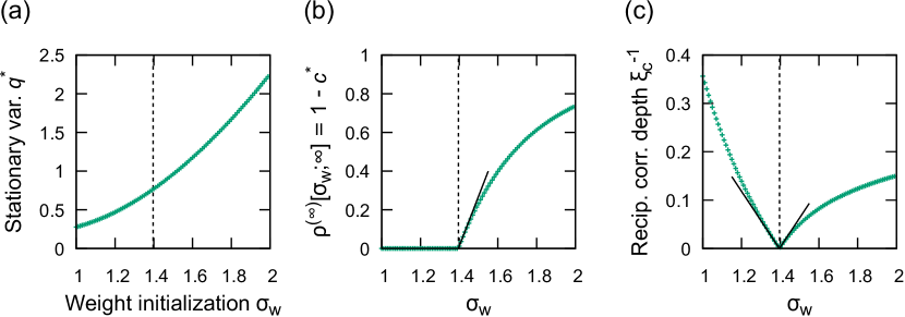
Figure 3: Quantitative characterization of the order-to-chaos transition in infinitely-wide FC. (a) The fixed point $q^{*}$ of the reucurrence relation (24) as a function of $\sigma_{w}$. (b) The fixed point $1-c^{*}$ of the recurrence relation (25) as a function of $\sigma_{w}$. The black solid line is guide-to-eye for linear onset, as expected from Eq. (47). (c) The reciprocal correlation depth $\xi_{c}^{-1}$, as calculated from Eq. (29). In all the three panels, $\sigma_{b}$ is set to be 0.3, and the vertical dashed lines indicate the poisition of the critical point $\sigma_{w;c}(\sim 1.3956)$ for that $\sigma_{b}$. The black solid lines are guide-to-eye for linear onset, as expected from Eq. (38) (left) and Eq. (40) (right).

Now let us prove the continuity of $q^{*}$ as a function of $\sigma_{w}$. As we stated in the main text, we expand the mean-field theory [12] with respect to infinitesimally small deviation $\delta\sigma_{w}$ from the critical point $\sigma_{w;c}$. Consider the fixed point $q^{*}$ of the mean-field theory (24) for infinitesimally different $\sigma_{w}$, and let $\delta\sigma_{w}$ and $\delta q^{*}$ respectively denote the increment in $\sigma_{w}$ and $q^{*}$. Then, we would like to find $\alpha>0$ such that

$$\delta q=\alpha\delta\sigma_{w}+O((\delta\sigma_{w})^{2}).$$ (32)

The following equality follows by the definition of $q^{*}$:

$$q^{*}=\sigma_{w}^{2}\int\mathrm{d}z\frac{1}{\sqrt{2\pi}}e^{-\frac{z^{2}}{2}}{}h^{2}(\sqrt{q^{*}}z)+\sigma_{b}^{2}$$ (33)

We expand the mean-field theory (24) to see the following (here we show the step-by-step calculations for demonstrations; after the equation below, straightforward deformations of formula are omitted in the proofs for brevity):

$$\begin{array}[]{rcl}q^{*}+\delta q^{*}&=&\displaystyle(\sigma_{w}+\delta\sigma_{w})^{2}\int\mathrm{d}z\frac{1}{\sqrt{2\pi}}e^{-\frac{z^{2}}{2}}{}h^{2}(\sqrt{q^{*}+\delta q^{*}}z)+\sigma_{b}^{2}\\ &=&\displaystyle\sigma_{w}^{2}\int\mathrm{d}z\frac{1}{\sqrt{2\pi}}e^{-\frac{z^{2}}{2}}{}\left[h(\sqrt{q^{*}}z)+\frac{\delta q^{*}z}{2\sqrt{q^{*}}}h^{\prime}(\sqrt{q^{*}}z)+O((\delta q^{*})^{2})\right]^{2}+\sigma_{b}^{2}\\ &&\displaystyle+2\sigma_{w}\delta\sigma_{w}\int\mathrm{d}z\frac{1}{\sqrt{2\pi}}e^{-\frac{z^{2}}{2}}h^{2}(\sqrt{q^{*}}z)+O((\delta\sigma_{w})^{2})\\ &=&\displaystyle\sigma_{w}^{2}\int\mathrm{d}z\frac{1}{\sqrt{2\pi}}e^{-\frac{z^{2}}{2}}{}h^{2}(\sqrt{q^{*}}z)+\sigma_{b}^{2}\\ &&\displaystyle+\delta q^{*}\cdot\frac{\sigma_{w}^{2}}{\sqrt{q^{*}}}\int\mathrm{d}z\frac{z}{\sqrt{2\pi}}e^{-\frac{z^{2}}{2}}{}h(\sqrt{q^{*}}z)h^{\prime}(\sqrt{q^{*}}z)\\ &&\displaystyle+2\sigma_{w}\delta\sigma_{w}\cdot\frac{q^{*}-\sigma_{b}^{2}}{\sigma_{w}^{2}}+O((\delta q^{*})^{2})+O((\delta\sigma_{w})^{2}).\end{array}$$ (34)

Subtracting Eq. (33) from Eq. (34) yields

$$\delta q^{*}{}=\delta q^{*}\sigma_{w}^{2}\int\mathrm{d}z\frac{z}{\sqrt{2\pi q^{*}{}}}e^{-\frac{z^{2}}{2}}h(\sqrt{q^{*}}z)h^{\prime}(\sqrt{q^{*}{}}z)+\frac{2(q^{*}-\sigma_{b}^{2})}{\sigma_{w}}\delta\sigma_{w},$$ (35)

from which we immediately find

$$\alpha=\frac{\displaystyle 2(q^{*}-\sigma_{b}^{2})}{\displaystyle\sigma_{w}\left[1-\sigma_{w}^{2}\int\mathrm{d}z\frac{z}{\sqrt{2\pi q^{*}}}e^{-\frac{z^{2}}{2}}h(\sqrt{q^{*}}z)h^{\prime}(\sqrt{q^{*}{}}z)\right]}.$$ (36)

In particular at the critical point $\sigma_{w;c}$, $\alpha$ can be further simplified to

$$\alpha=\frac{\displaystyle 2(q^{*}_{c}-\sigma_{b}^{2})}{\displaystyle-\sigma_{w}^{3}\int\mathrm{d}z\frac{1}{\sqrt{2\pi}}e^{-\frac{z^{2}}{2}}h(\sqrt{q^{*}_{c}}z)h^{\prime\prime}(\sqrt{q^{*}_{c}}z)},$$ (37)

where $q_{c}^{*}$ denotes the fixed point $q^{*}$ at the critical point. It turns out that the numerator and the denominator of the RHS of Eq. (36) converge to a finite value, and hence so does $\alpha$ itself.

Next we study the behavior of $\xi_{c}^{-1}$ around the critical point. To do this, we expand Eq. (29) with respect to an infinitesimal deviation $\delta\sigma_{w}$ from the critical point $\sigma_{w;c}$:

$$\begin{array}[]{rcl}e^{-\frac{1}{\xi_{c}(\sigma_{w;c}-\delta\sigma_{w})}}&=&\displaystyle(\sigma_{w;c}-\delta\sigma_{w})^{2}\int\mathrm{d}z\frac{1}{\sqrt{2\pi}}e^{-\frac{z^{2}}{2}}h^{\prime 2}(\sqrt{q_{c}^{*}-\alpha\delta\sigma_{w}}z)\\ &\sim&\displaystyle 1-\left[\frac{2}{\sigma_{w;c}}+\frac{\alpha\sigma_{w;c}^{2}}{\sqrt{q_{c}^{*}}}\int\mathrm{d}z\frac{z}{\sqrt{2\pi}}e^{-\frac{z^{2}}{2}}h^{\prime}(\sqrt{q_{c}^{*}}z)h^{\prime\prime}(\sqrt{q_{c}^{*}}z)\right]\delta\sigma_{w}.\\ \end{array}$$ (38)

The coefficient for $\delta\sigma_{w}$ in the RHS remains finite for the given activation function (namely $\tanh$), and hence one can see that $\xi_{c}^{-1}$ decreases to 0 as $\sigma_{w}\uparrow\sigma_{w;c}$ in an asymptotically linear manner, in particular

$$\iota_{1}=\frac{2}{\sigma_{w;c}}+\frac{\alpha\sigma_{w;c}^{2}}{\sqrt{q_{c}^{*}}}\int\mathrm{d}z\frac{z}{\sqrt{2\pi}}e^{-\frac{z^{2}}{2}}h^{\prime}(\sqrt{q_{c}^{*}}z)h^{\prime\prime}(\sqrt{q_{c}^{*}}z).$$ (39)

Similarly one finds

$$\begin{array}[]{rcl}e^{-\frac{1}{\xi_{c}(\sigma_{w;c}+\delta\sigma_{w})}}&=&\displaystyle(\sigma_{w;c}+\delta\sigma_{w})^{2}\int\mathrm{d}z_{2}\int\mathrm{d}z_{1}\frac{1}{\sqrt{(2\pi)^{2}}}e^{-\frac{z_{1}^{2}+z_{2}^{2}}{2}}h^{\prime}(u_{1}^{*}+\delta u_{1}^{*})h^{\prime}(u_{2}^{*}+\delta u_{2}^{*})\\ &\sim&\displaystyle 1-\left[\zeta\cdot\sigma_{w;c}^{2}q_{c}^{*}\int\mathrm{d}z\frac{1}{\sqrt{2\pi}}e^{-\frac{z^{2}}{2}}h^{\prime\prime 2}(\sqrt{q_{c}^{*}}z)-\iota_{1}\right]\delta\sigma_{w}\\ \end{array}$$ (40)

at the chaotic phase (assuming Eq. (30) holds), which indicates

$$\iota_{2}=\zeta\cdot\sigma_{w;c}^{2}q_{c}^{*}\int\mathrm{d}z\frac{1}{\sqrt{2\pi}}e^{-\frac{z^{2}}{2}}h^{\prime\prime 2}(\sqrt{q_{c}^{*}}z)-\iota_{1}.$$ (41)

Note that the contribution of order $\delta\sigma_{w}^{\frac{1}{2}}$ vanishes because

$$\int\mathrm{d}z\frac{z}{\sqrt{2\pi}}e^{-\frac{z^{2}}{2}}=0.$$ (42)

Thus it is confirmed that $\nu_{\|\mathrm{FC}}=1$.

To see the behavior of $c^{*}$ as a function of $\sigma_{w}$ in the chaotic phase, we expand the so-called $\mathcal{C}$-map (which can be obtained by setting $q_{1}^{(l)}=q_{2}^{(l)}=q^{*}$ in Eq. (25))

$$c^{(l+1)}=\frac{1}{q^{*}}\left[\sigma_{w}^{2}\int\mathrm{d}z_{1}\int\mathrm{d}z_{2}\frac{1}{\sqrt{(2\pi)^{2}}}e^{-\frac{z_{1}^{2}+z_{2}^{2}}{2}}h(u_{1}^{(l)})h(u_{2}^{(l)})+\sigma_{b}^{2}\right]$$ (43)

slightly above the critical point (that is, $\sigma_{w}=\sigma_{w;c}+\delta\sigma_{w}$) around the trivial fixed point $c^{(l)}=1$

$$c^{(l+1)}-c^{(l)}=\left(\left.\frac{\mathrm{d}c^{(l+1)}}{\mathrm{d}c^{(l)}}\right|_{c^{(l)=1}}-1\right)(c^{(l)}-1)+\frac{1}{2}\left.\frac{\mathrm{d}^{2}c^{(l+1)}}{\mathrm{d}c^{(l)2}}\right|_{c^{(l)}=1}(c^{(l)}-1)^{2}+\cdots,$$ (44)

because the straightforward expansion of the $\mathcal{C}$-map (43) around $\sigma_{w;c}$, as was done in the derivation of $\alpha$ (see Eq. (34)), yields a trivial identity ($0=0$). Notice that one can inductively see

$$\left.\frac{\mathrm{d}^{n}c^{(l+1)}}{\mathrm{d}c^{(l)n}}\right|_{c^{(l)}=1}=\sigma_{w}^{2}q^{*n-1}\int\mathrm{d}z\frac{1}{\sqrt{2\pi}}e^{-\frac{z^{2}}{2}}{}\left(\frac{\mathrm{d}^{n}h}{\mathrm{d}z^{n}}(\sqrt{q^{*}}z)\right)^{2},$$ (45)

which implies these derivatives are positive and finite at any order. Particularly in the vicinity of the critical point, we have

$$\left.\frac{\mathrm{d}c^{(l+1)}}{\mathrm{d}c^{(l)}}\right|_{c^{(l)}=1}-1=\iota_{1}\delta\sigma_{w}+o(\delta\sigma_{w}).$$ (46)

By taking the first two terms of the expansion (44) into account, one can see that the leading contribution for the nontrivial fixed point of the $\mathcal{C}$-map (43) is of order $\delta\sigma_{w}$ (and hence $\beta_{\mathrm{FC}}=1$), in particular

$$\zeta=\frac{2\iota_{1}}{\displaystyle\sigma_{w}^{2}q^{*}_{c}\int\mathrm{d}z\frac{1}{\sqrt{2\pi}}e^{-\frac{z^{2}}{2}}h^{\prime\prime 2}(\sqrt{q^{*}_{c}}z)}.$$ (47)

Remarkably, we find that the two coefficients $\iota_{1},\iota_{2}$ characterizing the power-law divergence of the correlation depth $\xi_{c}$ are identical with each other:

$$\iota_{1}=\iota_{2}(=:\iota).$$ (48)

To sum up, the order-to-chaos transition in untrained infinitely-wide FC with $\tanh$ activation can be characterized by the two critical exponents $\beta_{\mathrm{FC}}=1,\nu_{\|\mathrm{FC}}=1$ and three nonuniversal parameters $\sigma_{w;c},\iota,\zeta$. At this point, it is worthwhile to note that the parameters $\iota,\zeta$ are directly related to the parameters $\gamma(\tau),\kappa$ in the phenomenological description (9) in the main text; the order parameter $\rho^{(l)}$ as a function of depth $l$ can be described (to a reasonably good approximation, at least) by a solution of

$$\frac{\mathrm{d}\rho}{\mathrm{d}l}=\iota\cdot(\sigma_{w}-\sigma_{w;c})\rho-\frac{\iota}{\zeta}\rho^{2},$$ (49)

provided that the network is close enough to the critical point and that $l$ is sufficiently large.

References

- [1] David Silver, Aja Huang, Chris J. Maddison, Arthur Guez, Laurent Sifre, George van den Driessche, Julian Schrittwieser, Ioannis Antonoglou, Veda Panneershelvam, Marc Lanctot, Sander Dieleman, Dominik Grewe, John Nham, Nal Kalchbrenner, Ilya Sutskever, Timothy Lillicrap, Madeleine Leach, Koray Kavukcuoglu, Thore Graepel, and Demis Hassabis. Mastering the game of go with deep neural networks and tree search. Nature, 529(7587):484–489, Jan 2016.
- [2] Robin Rombach, Andreas Blattmann, Dominik Lorenz, Patrick Esser, and Björn Ommer. High-resolution image synthesis with latent diffusion models. In Proceedings of the IEEE/CVF Conference on Computer Vision and Pattern Recognition (CVPR), pages 10684–10695, June 2022.
- [3] Felix Stahlberg. Neural Machine Translation: A Review. Journal of Artificial Intelligence Research, 69:343–418, 2020.
- [4] Tom Henighan, Jared Kaplan, Mor Katz, Mark Chen, Christopher Hesse, Jacob Jackson, Heewoo Jun, Tom B. Brown, Prafulla Dhariwal, Scott Gray, Chris Hallacy, Benjamin Mann, Alec Radford, Aditya Ramesh, Nick Ryder, Daniel M. Ziegler, John Schulman, Dario Amodei, and Sam McCandlish. Scaling laws for autoregressive generative modeling. CoRR, abs/2010.14701, 2020.
- [5] Jared Kaplan, Sam McCandlish, Tom Henighan, Tom B. Brown, Benjamin Chess, Rewon Child, Scott Gray, Alec Radford, Jeffrey Wu, and Dario Amodei. Scaling laws for neural language models. CoRR, abs/2001.08361, 2020.
- [6] Xiaowei Xu, Yukun Ding, Sharon Xiaobo Hu, Michael Niemier, Jason Cong, Yu Hu, and Yiyu Shi. Scaling for edge inference of deep neural networks. Nature Electronics, 1(4):216–222, Apr 2018.
- [7] M. Henkel, H. Hinrichsen, and S. Lübeck. Non-Equilibrium Phase Transitions. Springer, 1st edition, 2008.
- [8] Haye Hinrichsen. Non-equilibrium critical phenomena and phase transitions into absorbing states. Advances in Physics, 49(7):815–958, 2000. arXiv: https://arxiv.org/abs/cond-mat/0001070.
- [9] Ronald Dickman, Alessandro Vespignani, and Stefano Zapperi. Self-organized criticality as an absorbing-state phase transition. Phys. Rev. E, 57:5095–5105, May 1998.
- [10] Mauricio Girardi-Schappo. Brain criticality beyond avalanches: open problems and how to approach them. Journal of Physics: Complexity, 2(3):031003, sep 2021.
- [11] H. Sompolinsky, A. Crisanti, and H. J. Sommers. Chaos in random neural networks. Phys. Rev. Lett., 61:259–262, Jul 1988.
- [12] Ben Poole, Subhaneil Lahiri, Maithra Raghu, Jascha Sohl-Dickstein, and Surya Ganguli. Exponential expressivity in deep neural networks through transient chaos. In D. Lee, M. Sugiyama, U. Luxburg, I. Guyon, and R. Garnett, editors, Advances in Neural Information Processing Systems, volume 29. Curran Associates, Inc., 2016.
- [13] Samuel S. Schoenholz, Justin Gilmer, Surya Ganguli, and Jascha Sohl-Dickstein. Deep Information Propagation. In International Conference on Learning Representations, 2017.
- [14] Daniel A. Roberts, Sho Yaida, and Boris Hanin. The Principles of Deep Learning Theory. Cambridge University Press, 2022. https://deeplearningtheory.com, arXiv: https://arxiv.org/abs/2106.10165.
- [15] Janina Hesse and Thilo Gross. Self-organized criticality as a fundamental property of neural systems. Frontiers in Systems Neuroscience, 8, 2014.
- [16] Soufiane Hayou, Arnaud Doucet, and Judith Rousseau. On the Impact of the Activation function on Deep Neural Networks Training. In Kamalika Chaudhuri and Ruslan Salakhutdinov, editors, Proceedings of the 36th International Conference on Machine Learning, volume 97 of Proceedings of Machine Learning Research, pages 2672–2680. PMLR, 09–15 Jun 2019.
- [17] Lechao Xiao, Yasaman Bahri, Jascha Sohl-Dickstein, Samuel Schoenholz, and Jeffrey Pennington. Dynamical Isometry and a Mean Field Theory of CNNs: How to Train 10,000-Layer Vanilla Convolutional Neural Networks. In Jennifer Dy and Andreas Krause, editors, Proceedings of the 35th International Conference on Machine Learning, volume 80 of Proceedings of Machine Learning Research, pages 5393–5402. PMLR, 2018.
- [18] Lechao Xiao, Jeffrey Pennington, and Samuel Schoenholz. Disentangling trainability and generalization in deep neural networks. In Hal Daumé III and Aarti Singh, editors, Proceedings of the 37th International Conference on Machine Learning, volume 119 of Proceedings of Machine Learning Research, pages 10462–10472. PMLR, 13–18 Jul 2020.
- [19] Gianbiagio Curato and Antonio Politi. Onset of chaotic dynamics in neural networks. Phys. Rev. E, 88:042908, Oct 2013.
- [20] Kazumasa A. Takeuchi, Masafumi Kuroda, Hugues Chaté, and Masaki Sano. Directed percolation criticality in turbulent liquid crystals. Phys. Rev. Lett., 99:234503, Dec 2007.
- [21] Kazumasa A. Takeuchi, Masafumi Kuroda, Hugues Chaté, and Masaki Sano. Experimental realization of directed percolation criticality in turbulent liquid crystals. Phys. Rev. E, 80:051116, Nov 2009.
- [22] T. E. Harris. Contact interactions on a lattice. The Annals of Probability, 2(6):969–988, 1974.
- [23] Kevin T. Grosvenor and Ro Jefferson. The edge of chaos: quantum field theory and deep neural networks. SciPost Phys., 12:081, 2022.
- [24] Sho Yaida. Non-Gaussian processes and neural networks at finite widths. In Jianfeng Lu and Rachel Ward, editors, Proceedings of The First Mathematical and Scientific Machine Learning Conference, volume 107 of Proceedings of Machine Learning Research, pages 165–192. PMLR, 20–24 Jul 2020.
- [25] John E. Kolassa. Edgeworth Series, pages 31–62. Springer New York, New York, NY, 2006.
- [26] S. R. Broadbent and J. M. Hammersley. Percolation processes: I. crystals and mazes. Mathematical Proceedings of the Cambridge Philosophical Society, 53(3):629â641, 1957.
- [27] Iwan Jensen. Low-density series expansions for directed percolation: I. a new efficient algorithm with applications to the square lattice. Journal of Physics A: Mathematical and General, 32(28):5233, jul 1999.
- [28] H. K. Janssen. On the nonequilibrium phase transition in reaction-diffusion systems with an absorbing stationary state. Zeitschrift für Physik B Condensed Matter, 42(2):151–154, Jun 1981.
- [29] P. Grassberger. On phase transitions in schlögl’s second model. Zeitschrift für Physik B Condensed Matter, 47(4):365–374, Dec 1982.
- [30] Christopher A. Voigt and Robert M. Ziff. Epidemic analysis of the second-order transition in the ziff-gulari-barshad surface-reaction model. Phys. Rev. E, 56:R6241–R6244, Dec 1997.
- [31] Junfeng Wang, Zongzheng Zhou, Qingquan Liu, Timothy M. Garoni, and Youjin Deng. High-precision monte carlo study of directed percolation in () dimensions. Phys. Rev. E, 88:042102, Oct 2013.
- [32] Andreas Messer and Haye Hinrichsen. Crossover from directed percolation to mean field behavior in the diffusive contact process. Journal of Statistical Mechanics: Theory and Experiment, 2008(04):P04024, 2008.
- [33] Arthur Jacot, Franck Gabriel, and Clement Hongler. Neural tangent kernel: Convergence and generalization in neural networks. In S. Bengio, H. Wallach, H. Larochelle, K. Grauman, N. Cesa-Bianchi, and R. Garnett, editors, Advances in Neural Information Processing Systems, volume 31. Curran Associates, Inc., 2018.
- [34] Lénaïc Chizat, Edouard Oyallon, and Francis Bach. On Lazy Training in Differentiable Programming. In H. Wallach, H. Larochelle, A. Beygelzimer, F. d'Alché-Buc, E. Fox, and R. Garnett, editors, Advances in Neural Information Processing Systems, volume 32. Curran Associates, Inc., 2019.
- [35] Boris Hanin and Mihai Nica. Finite Depth and Width Corrections to the Neural Tangent Kernel. In International Conference on Learning Representations, 2020.
- [36] Mariia Seleznova and Gitta Kutyniok. Neural Tangent Kernel Beyond the Infinite-Width Limit: Effects of Depth and Initialization. In Kamalika Chaudhuri, Stefanie Jegelka, Le Song, Csaba Szepesvari, Gang Niu, and Sivan Sabato, editors, Proceedings of the 39th International Conference on Machine Learning, volume 162 of Proceedings of Machine Learning Research, pages 19522–19560. PMLR, 17–23 Jul 2022.
- [37] A.J. Guttmann. Indicators of solvability for lattice models. Discrete Mathematics, 217(1):167–189, 2000.
- [38] Minmin Chen, Jeffrey Pennington, and Samuel Schoenholz. Dynamical isometry and a mean field theory of RNNs: Gating enables signal propagation in recurrent neural networks. In Jennifer Dy and Andreas Krause, editors, Proceedings of the 35th International Conference on Machine Learning, volume 80 of Proceedings of Machine Learning Research, pages 873–882. PMLR, 10–15 Jul 2018.
- [39] Ge Yang and Samuel Schoenholz. Mean field residual networks: On the edge of chaos. In I. Guyon, U. Von Luxburg, S. Bengio, H. Wallach, R. Fergus, S. Vishwanathan, and R. Garnett, editors, Advances in Neural Information Processing Systems, volume 30. Curran Associates, Inc., 2017.
- [40] Silvio R. Dahmen, Haye Hinrichsen, and Wolfgang Kinzel. Space representation of stochastic processes with delay. Phys. Rev. E, 77:031106, Mar 2008.
- [41] Marco Faggian, Francesco Ginelli, Francesco Marino, and Giovanni Giacomelli. Evidence of a critical phase transition in purely temporal dynamics with long-delayed feedback. Phys. Rev. Lett., 120:173901, Apr 2018.
- [42] Jaehoon Lee, Jascha Sohl-dickstein, Jeffrey Pennington, Roman Novak, Sam Schoenholz, and Yasaman Bahri. Deep Neural Networks as Gaussian Processes. In International Conference on Learning Representations, 2018.
- [43] Alexander G. de G. Matthews, Jiri Hron, Mark Rowland, Richard E. Turner, and Zoubin Ghahramani. Gaussian Process Behaviour in Wide Deep Neural Networks. In International Conference on Learning Representations, 2018.