Did we hear the sound of the Universe boiling?
Analysis using the full fluid velocity profiles and NANOGrav 15-year data

Abstract

In this paper, we analyse sound waves arising from a cosmic phase transition where the full velocity profile is taken into account as an explanation for the gravitational wave spectrum observed by multiple pulsar timing array groups. Unlike the broken power law used in the literature, in this scenario the power law after the peak depends on the macroscopic properties of the phase transition, allowing for a better fit with pulsar timing array (PTA) data. We compare the best fit with that obtained using the usual broken power law and, unsurprisingly, find a better fit with the gravitational wave (GW) spectrum that utilizes the full velocity profile. We then discuss models that can produce the best-fit point and complementary probes using CMB experiments and searches for light particles in DUNE, IceCUBE-Gen2, neutrinoless double $\beta-$decay, and forward physics facilities (FPF) at the LHC like FASER$\nu$, etc.

I Introduction

It has been known for some time that Pulsar Timing Array (PTA) experiments can be used to detect gravitational waves (GWs) Sazhin1978 ; Detweiler:1979wn ; Foster1990 . This is possible by studying the timing distortions of successive light pulses emitted by millisecond pulsars, which are extremely stable clocks. The PTAs search for spatially correlated fluctuations in the pulse arrival time measurements of such pulsars, due to GWs perturbing the space-time metric along the line of sight to each pulsar. For GWs, the timing distortions should exhibit the angular dependence expected for an isotropic background of spin two GWs which enables them to be distinguished from either spin-zero or spin-one waves, and other effects, according to the work of Hellings and Down Hellings:1983fr .

Recently, several PTA projects have reported the discovery of a stochastic gravitational wave background (SGWB). In particular, the North American Nanohertz Observatory for Gravitational Waves (NANOGrav) NANOGrav:2023gor , the European PTA Antoniadis:2023ott , the Parkes PTA Reardon:2023gzh and the Chinese CPTA Xu2023 have all released results which seem to be consistent with a Hellings-Downs pattern in the angular correlations which is characteristic of the SGWB. In particular, the largest statistical evidence for SGWB is seen in the NANOGrav 15-year data (NANOGrav15) NANOGrav:2023gor . This is the first discovery of GWs in the frequency around $10^{-8}$ Hz, and wavelengths around 10 light years. The most obvious origin of such an SGWB is due to the merging supermassive black hole binaries (SMBHBs) resulting from the collision of two galaxies, each with an SMBH with masses in the range $10^{8-9}$ solar masses at its centre Sesana:2004sp ; Burke-Spolaor:2018bvk . The expected amplitude has an order of magnitude uncertainty depending on the density, redshift, and other properties of SMBH sources. Indeed, there may be millions of such sources contributing to the SGWB.

However, the current data does not allow individual SMBH binary sources to be identified, so it is unclear if the observed SGWB has an astrophysical or cosmological origin Afzal2023 . For example, the cosmological origin of SGWB could be due to first-order phase transitions Winicour1973 ; Hogan:1986qda ; Caprini:2010xv ; NANOGrav:2021flc ; Xue:2021gyq ; DiBari:2021dri , cosmic strings Siemens:2006yp ; Ellis:2020ena ; King:2020hyd ; Buchmuller:2020lbh ; Blasi:2020mfx ; Bian:2022tju ; Fu:2023nrn , domain walls Ferreira:2022zzo ; An:2023idh ; Dunsky:2021tih , or scalar-induced gravitational waves (SIGWs) generated from primordial fluctuations Vaskonen:2020lbd ; DeLuca:2020agl ; Inomata:2020xad ; Sugiyama:2020roc ; Zhou:2020kkf ; Ghoshal:2023sfa . Such possibilities represent new physics beyond the standard model (BSM) and it would be interesting to know how such alternative scenarios could be distinguished.

One characteristic feature is the shape of the spectrum in the recent data, which, unlike the previous results, seems to be blue-tilted NANOGrav:2023gor ; Afzal2023 . The analysis of the NANOGrav 12.5-year data release suggested a nearly flat GW spectrum as a function of frequency ($f$), $\Omega_{GW}\propto f^{(-1.5,0.5)}$ at one sigma, in a narrow range of frequencies around 5.5 nHz NANOGrav:2020bcs . By contrast, the recent 15-year data release finds a steeper slope, $\Omega_{GW}\propto f^{(1.3,2.4)}$ at one sigma NANOGrav:2023gor . The naive scaling predicted for GW from SMBH binaries is disfavoured by the latest NANOGrav data, although environmental and statistical effects can lead to different predictions Afzal2023 ; Agazie2023 .

Motivated by the above considerations, new analyses are necessary to explore which SGWB formation mechanisms can lead to the generation of a signal consistent with these updated observations. Indeed, following the recent announcements, several papers have appeared which address some of these issues King:2023cgv ; Megias2023 ; Han2023 ; Guo2023 ; Yang2023 ; Kitajima2023 ; Bai2023 ; Zu2023 ; Kitajima2023a ; Vagnozzi2023 ; Lambiase2023 ; Ellis2023 ; Li2023 ; Franciolini2023 ; Shen2023 ; Ellis2023a ; Franciolini2023a ; Wang2023 ; Ghoshal2023 ; Fujikura2023 ; Athron:2023mer ; Kitajima:2023vre ; Lazarides:2023ksx ; Yang:2023qlf ; Addazi:2023jvg ; Broadhurst:2023tus ; Cai:2023dls ; Inomata:2023zup ; Depta:2023qst ; Depta:2023qst ; Eichhorn:2023gat ; Huang:2023chx ; Gouttenoire:2023ftk ; Blasi:2023sej .

In this paper, we consider the sound waves arising from a cosmic phase transition where the full velocity profile is taken into account. We compare the best fit with that obtained using the usual broken power law and find a better fit to NANOGrav data using the full velocity profile. We first explain how to obtain this result before discussing some models that can produce such thermal parameters. Finally, we discuss complementary probes of hidden sectors.

II PTA data and the sound shell model

Multiple PTA collaborations observed strong evidence for a gravitational wave spectrum, with NANOGrav and EPTA giving the best fit for a power law spectrum parametrized as follows,

$$\Omega=\frac{8\pi^{4}f^{5}\Phi(f)}{H_{0}^{2}\Delta f}$$ (1)

with

$$\Phi=\frac{A^{2}}{12\pi^{2}T_{\rm obs}}\left(\frac{f}{{\rm yr}^{-1}}\right)^{-\gamma}{\rm yr}^{3}$$ (2)

where $\Delta f=1/T_{\rm obs}$ and $H_{0}=h\times 100\,{\rm km}\,{\rm s}^{-1}{\rm Mpc}^{-1}$ is the current value of the Hubble rate. The best fit values of the parameters $A$ and $\gamma$ in Eq. 2 are given by

$$\gamma = \left\{\begin{array}[]{cc}3.2\pm 0.6&{\rm NANOGrav}\\ 3.1^{+0.77}_{-0.68}&{\rm EPTA}\end{array}\right.$$ (5)

$$A = \left\{\begin{array}[]{cc}6.4^{+4.2}_{-2.7}\times 10^{-15}&{\rm NANOGrav}\\ 10^{-14.13\pm 0.12}&{\rm EPTA}\end{array}\right.$$ (8)

While inspiralling SMBHBs provide the standard astrophysical explanation for the signal, a first-order phase transition (FOPT) at the $\mathcal{O}({\rm MeV})$ scale is an intriguing alternative. In this Section, we model the FOPT with the sound shell model Hindmarsh:2016lnk , obtain the corresponding GW spectrum, and compare our results with the fit performed by the NANOGrav Collaboration.

The GW spectrum from a FOPT is characterized by the following parameters: the nucleation temperature $T_{n}$, the strength of the FOPT $\alpha_{n}$, the average separation of bubbles $R_{n}$ which can be related to the bubble nucleation rate $\beta$, and the bubble wall velocity $v_{w}$. The fit frequently appearing in the literature, and in particular in the recent analysis of the NANOGrav paper describes a single broken power-law of the form Guo:2020grp ; Guo:2021qcq ; Caldwell:2022qsj ; Espinosa:2010hh ; Giese:2020rtr ; Hindmarsh:2016lnk ; Hindmarsh:2019phv ; Hindmarsh:2017gnf

$$h^{2}\Omega_{\text{GW}} = 8.5\times 10^{-6}\left(\frac{100}{g_{*}(T_{e})}\right)^{1/3}\Gamma^{2}\bar{U}_{f}^{4}\left[\frac{H_{s}}{\beta(v_{w})}\right]v_{w}\times\Upsilon$$ (9)

$$\times S(f),$$

where $\bar{U}_{f}$ is the root mean square fluid velocity, $\Gamma\sim 4/3$ is the adiabatic index and ${\Upsilon}$ is the suppression factor arising from the finite lifetime Ellis:2020awk ; Guo:2020grp ($\tau_{\text{sh}}$) of the sound waves Guo:2020grp

$$\Upsilon=1-\frac{1}{\sqrt{1+2\tau_{\text{sh}}H_{s}}}.$$ (10)

Finally, the spectral form has the shape

$$S(f)=\left(\frac{f}{f_{p}}\right)^{3}\left(\frac{7}{4+3(f/f_{p})^{2}}\right)^{7/2}$$ (11)

where $f_{p}$ is the peak frequency given by

$$f_{p}=8.9\times 10^{-6}\frac{1}{v_{w}}\left(\frac{\beta}{H_{e}}\right)\left(\frac{z_{p}}{10}\right)\left(\frac{T_{e}}{100{\rm GeV}}\right)\left(\frac{g_{\ast}(T_{e})}{100}\right)^{1/6}{\rm Hz}$$ (12)

However, a full calculation of the sound shell model can see qualitative deviations from this curve Hindmarsh:2019phv with a better fit being a double broken power law. Most important for our interests is the fact that the power law after the peak depends on the strength of the phase transition and the bubble wall velocity Gowling:2021gcy . A more optimistic scenario was studied in NANOGrav:2023hvm where the power law on either side of the peak was treated as a free parameter. In this work, we will perform a full calculation of the sound shell model to take advantage of this flexibility in the peak of the spectrum. Note that in the sound shell model, by keeping the force term between the bubble wall and the plasma longer, the shape can be modified in the infrared Cai:2023guc .

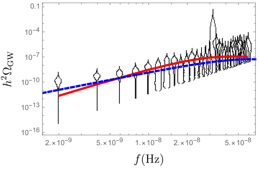
Figure 1: The data from NANOGrav measurement for relic density of SGWB w.r.t. frequency in Hz (black) against the best fit using the full sound shell model (red) and the best fit for a broken power law fit (blue) frequently appearing in the literature (see eqn 9). The parameters behind each fit are in Table 1.

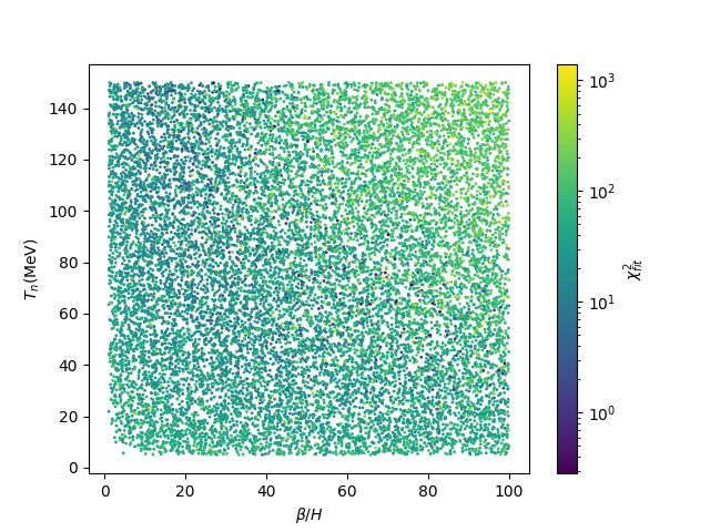
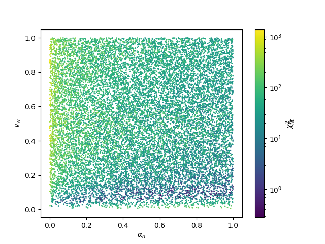
Figure 2: Scan over different parameters of FOPT: $T_{n}$, $\beta/H$, $v_{w}$ and $\alpha_{n}$ to find the minimum of $\chi_{\rm fit}^{2}$ for the best-fit point that matches the NANOGrav data for SGWB around $10^{-8}$ Hz.

Full Sound shell
Parameter	Best fit value
$\alpha_{n}$	0.85
$\beta/H_{\ast}$	42
$T_{n}$	133 MeV
$v_{w}$	0.09
$\chi_{\rm fit}$	1.4

Broken power law fit
Parameter	Best fit value
$\alpha_{n}$	0.89
$\beta/H_{\ast}$	5.17
$T_{n}$	142 MeV
$v_{w}$	0.67
$\chi_{\rm fit}$	1.59

Table 1: Best fit values for the full sound shell model and the usual fit used in the literature as given by Eq. 9. The full sound shell model performs somewhat better than the fit.

We will perform a scan over the space of thermal parameters, $(\alpha_{n},T_{n},v_{w},\beta/H_{n})$, to find the best fit to the NANOGrav data (who have released their full data including uncertainties). The scans are performed over the following ranges: nucleation temperature $3~{}\text{MeV}<T_{n}<150~{}\text{MeV}$, bubble wall velocity $0<v_{w}<1$, phase transition strength $0<\alpha_{n}<1$, and the efficiency of bubble formation w.r.t. the expansion rate $0<\beta/H<100$. Since the relevant ranges of temperature and frequency are around the quark-gluon confinement regime near $150$ MeV, we consider $g_{*}(T_{n})$ the evolution of degrees of freedom for the energy density of the thermal bath of SM particles at the nucleation temperature Drees:2015exa . The best fit point we use the following figure of merit

$$\chi_{\rm fit}^{2}=\sum_{i=1}^{N}\frac{\left(\log_{10}\Omega_{\rm th}h^{2}-\log_{10}\Omega_{\rm exp}h^{2}\right)^{2}}{2\bar{\sigma}_{i}^{2}}\,,$$ (13)

where $\Omega_{\rm th}h^{2}$ and $\Omega_{\rm exp}h^{2}$ represent the GW relic from theoretical prediction of FOPT and experimental value from PTA, respectively. Note that we ignore the width in the uncertainty regions, taking the midpoint and fitting to the vertical width. That is, $\sigma$, in the above equation is the distance from the midpoint value of $\log_{10}h^{2}\Omega_{\rm GW}$ for each uncertainty region to the top or bottom.

In Fig. 2 we display the results of our scan for data corresponding to NANOGrav.Using the data of NANOGrav we obtain the following values for the best fit point: $v_{w}\simeq 0.09$, $\alpha_{n}\simeq 0.85$, $T_{n}\simeq 132.95$ MeV and $\beta/H\simeq 42.02$.

III BSM Scenarios and Complementary Laboratory Probes

We are somewhat spoilt for choice in models that can produce a strong first order phase transition at roughly the QCD scale. The very large strength of the transition lends credit to solitosynthesis as a possible explanation Croon:2019rqu , as this mechanism typically leads to a stronger transition than conventional nucleation. The low wall velocity, however, supports a model that can predict a lot of friction like perhaps a SIMP model which can contain particles with large multiplicites Hochberg:2014dra ; Hochberg:2015vrg ; Garcia-Bellido:2021zgu ; Chakrabarty:2022yzp . Quite a few other dark sector phase transitions have been considered in this temperature range, see for instance  Breitbach:2018ddu ; Nakai:2020oit ; Ratzinger:2020koh ; Bai:2021ibt ; Bringmann:2023opz ; Deng:2023seh . Of course, while the QCD phase transition is a crossover in the standard model at low density, a high lepton asymmetry or a different number of light quarks can change this picture  Neronov:2020qrl ; Li:2021qer ; Sagunski:2023ynd . We focus here on a dark sectors that have the prospect of having complementary probes in searches for long lived particles. A full model survey we leave for future work.

Let us now briefly discuss model-independent constraints on a MeV scale FOPT in the dark or hidden sector. During a FOPT, the vacuum energy contained in the false vacuum gets released, and a part of it goes into reheating the photons or neutrinos in the plasma. The released energy may also end up heating relativistic particles in the dark sector. If the reheating of the SM particles happens at around or after the thermal decoupling of neutrinos and photons, either or both of their temperatures will differ from the predictions of standard cosmology. This will change the relativistic degrees of freedom, $N_{\text{eff}}$, which is strongly constrained by Big Bang Nucleosynthesis (BBN) and the Cosmic Microwave Background (CMB). The abundances of light element will also be modified and offer further bounds. $N_{\text{eff}}$ measurements severely constrain the dark sector reheating scenario as well. While our best fit point has a percolation temperature well above the scale at which we need to be concerned with BBN constraints, there are some points the agree well with NANOGrav data and have a much lower percolation temperature.

We first consider the reheating of the dark radiation case. In the approximation $T_{n}^{D}\ll T_{n}^{\gamma}$, one can show that $\alpha_{n}<0.08$ for $T_{n}^{\gamma}\sim\mathcal{O}$(MeV) Bai:2021ibt . Ref. Bai:2021ibt also derived model-independent constraints on phase temperature ($T_{n}$) and strength parameter ($\alpha_{n}$) from $N_{\text{eff}}$ and helium and primary deuterium abundance ratios ($Y_{P}$ and $D/H|_{P}$, respectively) measured by CMB and BBN experiments when the FOPT heats the SM particles. For illustration, we discuss here the neutrino reheating scenario since the portal operator that can induce it (and the associated phenomenology) is relatively well-studied Berryman:2022hds .

Using the BBN data from PDG ParticleDataGroup:2020ssz and the CMB data from the latest Planck results Planck:2019nip , Ref. Bai:2021ibt shows that the neutrino reheating temperature, $T^{\nu}_{\text{rh}}$, has to be greater than $\sim 3$ MeV for $\alpha_{n}>0.1$. A future CMB experiment like CMB-S4 Abazajian:2019eic will improve the bounds to $T^{\nu}_{\text{rh}}\gtrsim 4$ MeV. One can translate the above bounds on $T^{\nu}_{\text{rh}}$ to the phase transition temperature $T_{n}$ by using the formula,

$$T^{\nu}_{\text{rh}}=\bigg{[}1\,+\,\alpha_{n}\,+\,\alpha_{n}\frac{g_{*}^{\gamma}(t_{{\text{rh}}})}{g_{*}^{\nu}(t_{\text{rh}})}\Big{(}\frac{T_{n}^{\gamma}}{T_{n}^{\nu}}\Big{)}^{4}\bigg{]}^{1/4}\,T_{n}^{\nu}\,\,,$$ (14)

where for reheating temperatures above MeV, $g_{*}^{\gamma}(t_{{\text{rh}}})\approx 11/2$ and $g_{*}^{\nu}(t_{{\text{rh}}})\approx 21/4$. Thus, one can conclude that the existing CMB and BBN data bounds place an almost flat constraint on $T_{n}^{\nu}\gtrsim 2$ MeV for $\alpha_{n}>0.1$ as shown by the blue line in Fig. 3. The bound on $T_{n}$ from the photon reheating case is almost the same but extends to a bit smaller values of $\alpha_{n}$ Bai:2021ibt .

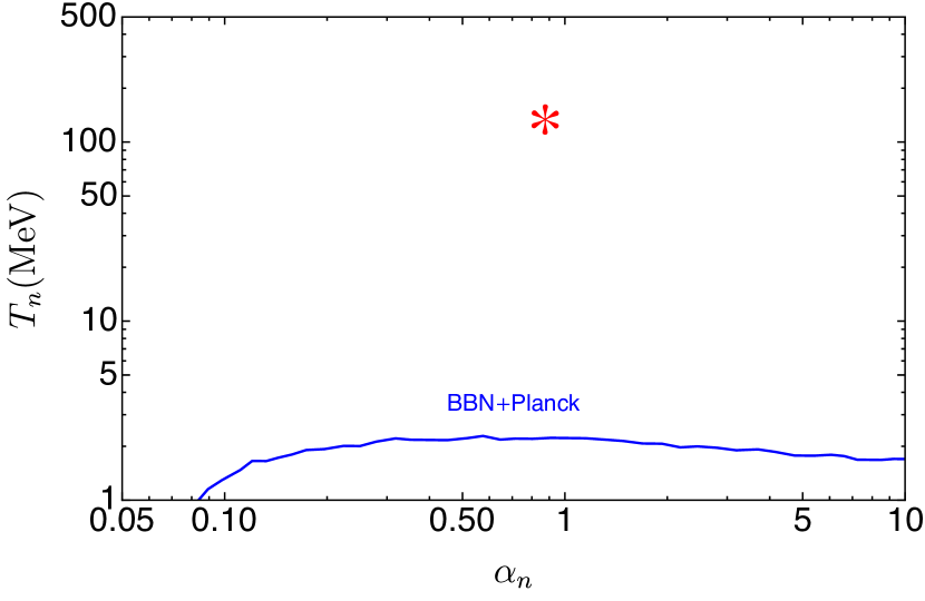
Figure 3: Constraints on FOPT parameters from PLANCK and BBN taken from Ref. Bai:2021ibt . The best-fit point obtained from our sound shell analysis with the NANOGrav data is shown by the red star.

Finally, we provide a brief discussion on the interactions between the SM neutrinos and the dark sector scalar that is responsible for the FOPT under discussion. There is one point that we should clarify that the reheating has to be instantaneous for the above constraints to be applicable. For a delayed reheating, the constraints on the FOPT is expected be much stronger Bai:2021ibt . The neutrino reheating can happen from the decay of a dark scalar $\phi$ to a pair of neutrinos via the dimension-6 effective operator

$$\mathcal{O}=\lambda_{\alpha\beta}\,\frac{(L^{T}_{\alpha}i\sigma_{2}H)(H^{T}i\sigma_{2}L_{\beta})\phi}{\Lambda^{2}},$$ (15)

where $L$ and $H$ are the SM lepton and Higgs doublets, respectively. After the electroweak symmetry breaking the above operator will generate an interaction term $g_{\alpha\beta}\,{\nu}\nu\phi$, where $\alpha,\beta=e,\mu,\tau$ and $g_{\alpha\beta}=\lambda_{\alpha\beta}\,v^{2}/\Lambda^{2}$. Significant bounds already exists on the $g_{\alpha\beta}-m_{\phi}$ plane from existing laboratory experiments like meson decay spectra Pasquini:2015fjv , neutrinoless double $\beta$-decay Brune:2018sab , $Z$ or the SM Higgs invisible decay or $\tau$ decay deGouvea:2019qaz . Also, these couplings are significant interest of study in upcoming experiments like DUNEBerryman:2018ogk ; Kelly:2021mcd , generation-2 IceCube Cherry:2014xra , and forward physics facilities (FPF) Kelly:2021mcd at the LHC. We show a subset of these existing and projected bounds on the $g_{\alpha\beta}-m_{\phi}$ plane in Fig. 4. For the detailed phenomenology of these couplings at various terrestrial and celestial experiments we refer the interested readers to the recent review paper on this topic Berryman:2022hds . As far as the UV-completion of the effective operator of Eq. 15 is concerned, the most canonical models that can provide it are the massive Majoron models Rothstein:1992rh ; Gu:2010ys ; Queiroz:2014yna ; Brune:2018sab . In addition, the generation of this effective operator from an inverse seesaw model Lyu:2020lps and a $U(1)_{B-L}$ Dev:2021axj model has been considered in the literature.

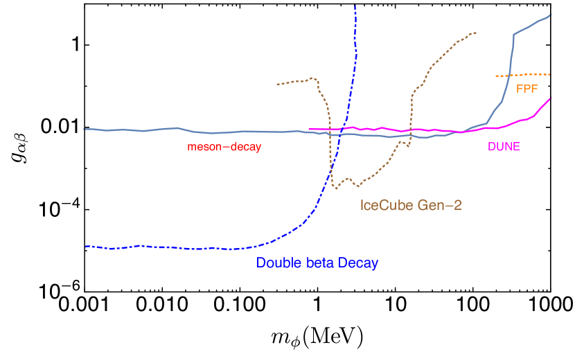
Figure 4: A selection of limits on the parameters $g_{\alpha\beta}$ and $m_{\phi}$ that can participate in reheating the neutrino plasma from the decay of a dark sector scalar. We show the existing laboratory constraints from meson decay spectra [dark blue solid] and neutrinoless double $\beta$-decay [blue dot dashed]. Also we show the projected limits from DUNE [magenta solid], IceCube Gen-2 [brown dotted] and forward physics facility at the LHC [orange dotted].

IV Discussions and Conclusions

In this paper we have had an in depth look at sound wave induced gravitational waves from a strong first order cosmic phase transition as a possible explanation for the recent signal at multiple pulsar timing arrays. In particular, we have looked at how much including the full velocity profile rather than using a broken power law fit improves agreement with data. The best fit parameters also look a bit more realistic than what can be achieved via the broken power law, with the time scale of the phase transition being a smaller fraction of the Hubble time. We of course emphasize the caveat that understanding the spectrum from sound shell models is still in a state of flux. Reheating can suppress the nucelation rate enhancing the spectrum Jinno:2021ury . On the other hand, energy lost to vorticity can suppress the spectrum Cutting:2019zws . We leave a detailed analysis of this to future work. We then took a brief look at dark sector models that can be responsible for such a phase transition. We show that one for phase transitions occurring at low temperatures, the cosmological constraints from BBN, PLANCK data and future sensitivities from CMB experiments like CMB-S4, CMB-HD, CMB-Bharat, LiteBIRD will be complementary to the gravitational wave detectors to essential probe phase transition parameter space. This complementarity approach to probe phase transitions via GW detectors as well as CMB detectors paves the way distinguish the SMBHB and phase transition explanations to observed gravitational waves. Furthermore we showed that once we fix an operator that decides the interactions between the SM sector and the invisible sector (Eqn. 11) one is able to search for such mediators which is responsible for such interactions. We also discussed possible UV-complete neutrino mass models that can give rise to such low scale phase transitions and GW from sound waves measured in PTA data however detailed analysis involving a complete UV-complete model is beyond the scope of the current paper and will be taken up in a future publication. We envisage that the precision measurements that the GW cosmology and GW astronomy offers us from current data and from the planned worldwide network of GW detectors will make the dream of testing particle physics and fundamental BSM scenarios a reality in the very near future.

Acknowledgments

The work of T.G. is supported by the funding available from the Department of Atomic Energy (DAE), Government of India for Harish-Chandra Research Institute. A.G. thanks hospitality of University of Pisa during the ongoing work. SFK acknowledges the STFC Consolidated Grant ST/L000296/1 and the European Union’s Horizon 2020 Research and Innovation programme under Marie Sklodowska-Curie grant agreement HIDDeN European ITN project (H2020-MSCA-ITN-2019//860881-HIDDeN). KS is supported by the U. S. Department of Energy grant DE-SC0009956. XW acknowledges the Royal Society as the funding source of the Newton International Fellowship.

References

- (1) M. V. Sazhin, “Opportunities for detecting ultralong gravitational waves,” Soviet Astronomy 22 (Feb., 1978) 36–38.
- (2) S. L. Detweiler, “Pulsar timing measurements and the search for gravitational waves,” Astrophys. J. 234 (1979) 1100–1104.
- (3) R. S. Foster and D. C. Backer, “Constructing a Pulsar Timing Array,” Astrophys. J. 361 (Sept., 1990) 300.
- (4) R. w. Hellings and G. s. Downs, “UPPER LIMITS ON THE ISOTROPIC GRAVITATIONAL RADIATION BACKGROUND FROM PULSAR TIMING ANALYSIS,” Astrophys. J. Lett. 265 (1983) L39–L42.
- (5) NANOGrav Collaboration, G. Agazie et al., “The NANOGrav 15-year Data Set: Evidence for a Gravitational-Wave Background,” Astrophys. J. Lett. 951 no. 1, (2023) , arXiv:2306.16213 [astro-ph.HE].
- (6) J. Antoniadis et al., “The second data release from the European Pulsar Timing Array III. Search for gravitational wave signals,” arXiv:2306.16214 [astro-ph.HE].
- (7) D. J. Reardon et al., “Search for an isotropic gravitational-wave background with the Parkes Pulsar Timing Array,” Astrophys. J. Lett. 951 no. 1, (2023) , arXiv:2306.16215 [astro-ph.HE].
- (8) H. Xu, S. Chen, et al., “Searching for the nano-hertz stochastic gravitational wave background with the chinese pulsar timing array data release i,” arXiv:2306.16216 [astro-ph.HE].
- (9) A. Sesana, F. Haardt, P. Madau, and M. Volonteri, “Low - frequency gravitational radiation from coalescing massive black hole binaries in hierarchical cosmologies,” Astrophys. J. 611 (2004) 623–632, arXiv:astro-ph/0401543.
- (10) S. Burke-Spolaor et al., “The Astrophysics of Nanohertz Gravitational Waves,” Astron. Astrophys. Rev. 27 no. 1, (2019) 5, arXiv:1811.08826 [astro-ph.HE].
- (11) A. Afzal, G. Agazie, et al., “The nanograv 15-year data set: Search for signals from new physics,” arXiv:2306.16219 [astro-ph.HE].
- (12) J. Winicour, “Gravitational Radiation from Relativistic Phase Transitions,” Astrophys. J. 182 (June, 1973) 919–934.
- (13) C. J. Hogan, “Gravitational radiation from cosmological phase transitions,” Mon. Not. Roy. Astron. Soc. 218 (1986) 629–636.
- (14) C. Caprini, R. Durrer, and X. Siemens, “Detection of gravitational waves from the QCD phase transition with pulsar timing arrays,” Phys. Rev. D 82 (2010) 063511, arXiv:1007.1218 [astro-ph.CO].
- (15) NANOGrav Collaboration, Z. Arzoumanian et al., “Searching for Gravitational Waves from Cosmological Phase Transitions with the NANOGrav 12.5-Year Dataset,” Phys. Rev. Lett. 127 no. 25, (2021) 251302, arXiv:2104.13930 [astro-ph.CO].
- (16) X. Xue et al., “Constraining Cosmological Phase Transitions with the Parkes Pulsar Timing Array,” Phys. Rev. Lett. 127 no. 25, (2021) 251303, arXiv:2110.03096 [astro-ph.CO].
- (17) P. Di Bari, D. Marfatia, and Y.-L. Zhou, “Gravitational waves from first-order phase transitions in Majoron models of neutrino mass,” JHEP 10 (2021) 193, arXiv:2106.00025 [hep-ph].
- (18) X. Siemens, V. Mandic, and J. Creighton, “Gravitational wave stochastic background from cosmic (super)strings,” Phys. Rev. Lett. 98 (2007) 111101, arXiv:astro-ph/0610920.
- (19) J. Ellis and M. Lewicki, “Cosmic String Interpretation of NANOGrav Pulsar Timing Data,” Phys. Rev. Lett. 126 no. 4, (2021) 041304, arXiv:2009.06555 [astro-ph.CO].
- (20) S. F. King, S. Pascoli, J. Turner, and Y.-L. Zhou, “Gravitational Waves and Proton Decay: Complementary Windows into Grand Unified Theories,” Phys. Rev. Lett. 126 no. 2, (2021) 021802, arXiv:2005.13549 [hep-ph].
- (21) W. Buchmuller, V. Domcke, and K. Schmitz, “From NANOGrav to LIGO with metastable cosmic strings,” Phys. Lett. B 811 (2020) 135914, arXiv:2009.10649 [astro-ph.CO].
- (22) S. Blasi, V. Brdar, and K. Schmitz, “Has NANOGrav found first evidence for cosmic strings?,” Phys. Rev. Lett. 126 no. 4, (2021) 041305, arXiv:2009.06607 [astro-ph.CO].
- (23) L. Bian, J. Shu, B. Wang, Q. Yuan, and J. Zong, “Searching for cosmic string induced stochastic gravitational wave background with the Parkes Pulsar Timing Array,” Phys. Rev. D 106 no. 10, (2022) L101301, arXiv:2205.07293 [hep-ph].
- (24) B. Fu, A. Ghoshal, and S. King, “Cosmic string gravitational waves from global symmetry breaking as a probe of the type I seesaw scale,” arXiv:2306.07334 [hep-ph].
- (25) R. Z. Ferreira, A. Notari, O. Pujolas, and F. Rompineve, “Gravitational waves from domain walls in Pulsar Timing Array datasets,” JCAP 02 (2023) 001, arXiv:2204.04228 [astro-ph.CO].
- (26) H. An and C. Yang, “Gravitational Waves Produced by Domain Walls During Inflation,” arXiv:2304.02361 [hep-ph].
- (27) D. I. Dunsky, A. Ghoshal, H. Murayama, Y. Sakakihara, and G. White, “GUTs, hybrid topological defects, and gravitational waves,” Phys. Rev. D 106 no. 7, (2022) 075030, arXiv:2111.08750 [hep-ph].
- (28) V. Vaskonen and H. Veermäe, “Did NANOGrav see a signal from primordial black hole formation?,” Phys. Rev. Lett. 126 no. 5, (2021) 051303, arXiv:2009.07832 [astro-ph.CO].
- (29) V. De Luca, G. Franciolini, and A. Riotto, “NANOGrav Data Hints at Primordial Black Holes as Dark Matter,” Phys. Rev. Lett. 126 no. 4, (2021) 041303, arXiv:2009.08268 [astro-ph.CO].
- (30) K. Inomata, M. Kawasaki, K. Mukaida, and T. T. Yanagida, “NANOGrav Results and LIGO-Virgo Primordial Black Holes in Axionlike Curvaton Models,” Phys. Rev. Lett. 126 no. 13, (2021) 131301, arXiv:2011.01270 [astro-ph.CO].
- (31) S. Sugiyama, V. Takhistov, E. Vitagliano, A. Kusenko, M. Sasaki, and M. Takada, “Testing Stochastic Gravitational Wave Signals from Primordial Black Holes with Optical Telescopes,” Phys. Lett. B 814 (2021) 136097, arXiv:2010.02189 [astro-ph.CO].
- (32) Z. Zhou, J. Jiang, Y.-F. Cai, M. Sasaki, and S. Pi, “Primordial black holes and gravitational waves from resonant amplification during inflation,” Phys. Rev. D 102 no. 10, (2020) 103527, arXiv:2010.03537 [astro-ph.CO].
- (33) A. Ghoshal, Y. Gouttenoire, L. Heurtier, and P. Simakachorn, “Primordial Black Hole Archaeology with Gravitational Waves from Cosmic Strings,” arXiv:2304.04793 [hep-ph].
- (34) NANOGrav Collaboration, Z. Arzoumanian et al., “The NANOGrav 12.5 yr Data Set: Search for an Isotropic Stochastic Gravitational-wave Background,” Astrophys. J. Lett. 905 no. 2, (2020) L34, arXiv:2009.04496 [astro-ph.HE].
- (35) G. Agazie, A. Anumarlapudi, et al., “The nanograv 15-year data set: Constraints on supermassive black hole binaries from the gravitational wave background,” arXiv:2306.16220 [astro-ph.HE].
- (36) S. F. King, D. Marfatia, and M. H. Rahat, “Towards distinguishing Dirac from Majorana neutrino mass with gravitational waves,” arXiv:2306.05389 [hep-ph].
- (37) E. Megias, G. Nardini, and M. Quiros, “Pulsar timing array stochastic background from light kaluza-klein resonances,” arXiv:2306.17071 [hep-ph].
- (38) C. Han, K.-P. Xie, J. M. Yang, and M. Zhang, “Self-interacting dark matter implied by nano-hertz gravitational waves,” arXiv:2306.16966 [hep-ph].
- (39) S.-Y. Guo, M. Khlopov, X. Liu, L. Wu, Y. Wu, and B. Zhu, “Footprints of axion-like particle in pulsar timing array data and jwst observations,” arXiv:2306.17022 [hep-ph].
- (40) J. Yang, N. Xie, and F. P. Huang, “Nano-hertz stochastic gravitational wave background as hints of ultralight axion particles,” arXiv:2306.17113 [hep-ph].
- (41) N. Kitajima, J. Lee, K. Murai, F. Takahashi, and W. Yin, “Nanohertz gravitational waves from axion domain walls coupled to qcd,” arXiv:2306.17146 [hep-ph].
- (42) Y. Bai, T.-K. Chen, and M. Korwar, “Qcd-collapsed domain walls: Qcd phase transition and gravitational wave spectroscopy,” arXiv:2306.17160 [hep-ph].
- (43) L. Zu, C. Zhang, Y.-Y. Li, Y.-C. Gu, Y.-L. S. Tsai, and Y.-Z. Fan, “Mirror qcd phase transition as the origin of the nanohertz stochastic gravitational-wave background detected by the pulsar timing arrays,” arXiv:2306.16769 [astro-ph.HE].
- (44) N. Kitajima and T. Takahashi, “Stochastic gravitational wave background from early dark energy,” arXiv:2306.16896 [astro-ph.CO].
- (45) S. Vagnozzi, “Inflationary interpretation of the stochastic gravitational wave background signal detected by pulsar timing array experiments,” arXiv:2306.16912 [astro-ph.CO].
- (46) G. Lambiase, L. Mastrototaro, and L. Visinelli, “Astrophysical neutrino oscillations after pulsar timing array analyses,” arXiv:2306.16977 [astro-ph.HE].
- (47) J. Ellis, M. Fairbairn, G. Hütsi, J. Raidal, J. Urrutia, V. Vaskonen, and H. Veermäe, “Gravitational waves from smbh binaries in light of the nanograv 15-year data,” arXiv:2306.17021 [astro-ph.CO].
- (48) Y. Li, C. Zhang, Z. Wang, M. Cui, Y.-L. S. Tsai, Q. Yuan, and Y.-Z. Fan, “Primordial magnetic field as a common solution of nanohertz gravitational waves and hubble tension,” arXiv:2306.17124 [astro-ph.HE].
- (49) G. Franciolini, D. Racco, and F. Rompineve, “Footprints of the qcd crossover on cosmological gravitational waves at pulsar timing arrays,” arXiv:2306.17136 [astro-ph.CO].
- (50) Z.-Q. Shen, G.-W. Yuan, Y.-Y. Wang, and Y.-Z. Wang, “Dark matter spike surrounding supermassive black holes binary and the nanohertz stochastic gravitational wave background,” arXiv:2306.17143 [astro-ph.HE].
- (51) J. Ellis, M. Lewicki, C. Lin, and V. Vaskonen, “Cosmic superstrings revisited in light of nanograv 15-year data,” arXiv:2306.17147 [astro-ph.CO].
- (52) G. Franciolini, A. J. Iovino, V. Vaskonen, and H. Veermae, “The recent gravitational wave observation by pulsar timing arrays and primordial black holes: the importance of non-gaussianities,” arXiv:2306.17149 [astro-ph.CO].
- (53) Z. Wang, L. Lei, H. Jiao, L. Feng, and Y.-Z. Fan, “The nanohertz stochastic gravitational-wave background from cosmic string loops and the abundant high redshift massive galaxies,” arXiv:2306.17150 [astro-ph.HE].
- (54) A. Ghoshal and A. Strumia, “Probing the dark matter density with gravitational waves from super-massive binary black holes,” arXiv:2306.17158 [astro-ph.CO].
- (55) K. Fujikura, S. Girmohanta, Y. Nakai, and M. Suzuki, “Nanograv signal from a dark conformal phase transition,” arXiv:2306.17086 [hep-ph].
- (56) P. Athron, A. Fowlie, C.-T. Lu, L. Morris, L. Wu, Z. Xu, and Y. Wu, “Can Supercooled Phase Transitions explain the Gravitational Wave Background observed by Pulsar Timing Arrays?,” arXiv:2306.17239 [hep-ph].
- (57) N. Kitajima and K. Nakayama, “Nanohertz gravitational waves from cosmic strings and dark photon dark matter,” arXiv:2306.17390 [hep-ph].
- (58) G. Lazarides, R. Maji, and Q. Shafi, “Superheavy quasi-stable strings and walls bounded by strings in the light of NANOGrav 15 year data,” arXiv:2306.17788 [hep-ph].
- (59) A. Yang, J. Ma, S. Jiang, and F. P. Huang, “Implication of nano-Hertz stochastic gravitational wave on dynamical dark matter through a first-order phase transition,” arXiv:2306.17827 [hep-ph].
- (60) A. Addazi, Y.-F. Cai, A. Marciano, and L. Visinelli, “Have pulsar timing array methods detected a cosmological phase transition?,” arXiv:2306.17205 [astro-ph.CO].
- (61) T. Broadhurst, C. Chen, T. Liu, and K.-F. Zheng, “Binary Supermassive Black Holes Orbiting Dark Matter Solitons: From the Dual AGN in UGC4211 to NanoHertz Gravitational Waves,” arXiv:2306.17821 [astro-ph.HE].
- (62) Y.-F. Cai, X.-C. He, X. Ma, S.-F. Yan, and G.-W. Yuan, “Limits on scalar-induced gravitational waves from the stochastic background by pulsar timing array observations,” arXiv:2306.17822 [gr-qc].
- (63) K. Inomata, K. Kohri, and T. Terada, “The Detected Stochastic Gravitational Waves and Sub-Solar Primordial Black Holes,” arXiv:2306.17834 [astro-ph.CO].
- (64) P. F. Depta, K. Schmidt-Hoberg, and C. Tasillo, “Do pulsar timing arrays observe merging primordial black holes?,” arXiv:2306.17836 [astro-ph.CO].
- (65) A. Eichhorn, R. R. Lino dos Santos, and J. a. L. Miqueleto, “From quantum gravity to gravitational waves through cosmic strings,” arXiv:2306.17718 [gr-qc].
- (66) H.-L. Huang, Y. Cai, J.-Q. Jiang, J. Zhang, and Y.-S. Piao, “Supermassive primordial black holes in multiverse: for nano-Hertz gravitational wave and high-redshift JWST galaxies,” arXiv:2306.17577 [gr-qc].
- (67) Y. Gouttenoire and E. Vitagliano, “Domain wall interpretation of the PTA signal confronting black hole overproduction,” arXiv:2306.17841 [gr-qc].
- (68) S. Blasi, A. Mariotti, A. Rase, and A. Sevrin, “Axionic domain walls at Pulsar Timing Arrays: QCD bias and particle friction,” arXiv:2306.17830 [hep-ph].
- (69) M. Hindmarsh, “Sound shell model for acoustic gravitational wave production at a first-order phase transition in the early Universe,” Phys. Rev. Lett. 120 no. 7, (2018) 071301, arXiv:1608.04735 [astro-ph.CO].
- (70) H.-K. Guo, K. Sinha, D. Vagie, and G. White, “Phase Transitions in an Expanding Universe: Stochastic Gravitational Waves in Standard and Non-Standard Histories,” JCAP 01 (2021) 001, arXiv:2007.08537 [hep-ph].
- (71) H.-K. Guo, K. Sinha, D. Vagie, and G. White, “The benefits of diligence: how precise are predicted gravitational wave spectra in models with phase transitions?,” JHEP 06 (2021) 164, arXiv:2103.06933 [hep-ph].
- (72) R. Caldwell et al., “Detection of early-universe gravitational-wave signatures and fundamental physics,” Gen. Rel. Grav. 54 no. 12, (2022) 156, arXiv:2203.07972 [gr-qc].
- (73) J. R. Espinosa, T. Konstandin, J. M. No, and G. Servant, “Energy Budget of Cosmological First-order Phase Transitions,” JCAP 06 (2010) 028, arXiv:1004.4187 [hep-ph].
- (74) F. Giese, T. Konstandin, and J. van de Vis, “Model-independent energy budget of cosmological first-order phase transitions—A sound argument to go beyond the bag model,” JCAP 07 no. 07, (2020) 057, arXiv:2004.06995 [astro-ph.CO].
- (75) M. Hindmarsh and M. Hijazi, “Gravitational waves from first order cosmological phase transitions in the Sound Shell Model,” JCAP 12 (2019) 062, arXiv:1909.10040 [astro-ph.CO].
- (76) M. Hindmarsh, S. J. Huber, K. Rummukainen, and D. J. Weir, “Shape of the acoustic gravitational wave power spectrum from a first order phase transition,” Phys. Rev. D 96 no. 10, (2017) 103520, arXiv:1704.05871 [astro-ph.CO]. [Erratum: Phys.Rev.D 101, 089902 (2020)].
- (77) J. Ellis, M. Lewicki, and J. M. No, “Gravitational waves from first-order cosmological phase transitions: lifetime of the sound wave source,” JCAP 07 (2020) 050, arXiv:2003.07360 [hep-ph].
- (78) C. Gowling and M. Hindmarsh, “Observational prospects for phase transitions at LISA: Fisher matrix analysis,” JCAP 10 (2021) 039, arXiv:2106.05984 [astro-ph.CO].
- (79) NANOGrav Collaboration, A. Afzal et al., “The NANOGrav 15 yr Data Set: Search for Signals from New Physics,” Astrophys. J. Lett. 951 no. 1, (2023) L11, arXiv:2306.16219 [astro-ph.HE].
- (80) R.-G. Cai, S.-J. Wang, and Z.-Y. Yuwen, “Hydrodynamic sound shell model,” arXiv:2305.00074 [gr-qc].
- (81) M. Drees, F. Hajkarim, and E. R. Schmitz, “The Effects of QCD Equation of State on the Relic Density of WIMP Dark Matter,” JCAP 06 (2015) 025, arXiv:1503.03513 [hep-ph].
- (82) D. Croon, A. Kusenko, A. Mazumdar, and G. White, “Solitosynthesis and Gravitational Waves,” Phys. Rev. D 101 no. 8, (2020) 085010, arXiv:1910.09562 [hep-ph].
- (83) Y. Hochberg, E. Kuflik, T. Volansky, and J. G. Wacker, “Mechanism for Thermal Relic Dark Matter of Strongly Interacting Massive Particles,” Phys. Rev. Lett. 113 (2014) 171301, arXiv:1402.5143 [hep-ph].
- (84) Y. Hochberg, E. Kuflik, and H. Murayama, “SIMP Spectroscopy,” JHEP 05 (2016) 090, arXiv:1512.07917 [hep-ph].
- (85) J. Garcia-Bellido, H. Murayama, and G. White, “Exploring the early Universe with Gaia and Theia,” JCAP 12 no. 12, (2021) 023, arXiv:2104.04778 [hep-ph].
- (86) N. Chakrabarty, H. Roy, and T. Srivastava, “Single-step first order phase transition and gravitational waves in a SIMP dark matter scenario,” arXiv:2212.09659 [hep-ph].
- (87) M. Breitbach, J. Kopp, E. Madge, T. Opferkuch, and P. Schwaller, “Dark, Cold, and Noisy: Constraining Secluded Hidden Sectors with Gravitational Waves,” JCAP 07 (2019) 007, arXiv:1811.11175 [hep-ph].
- (88) Y. Nakai, M. Suzuki, F. Takahashi, and M. Yamada, “Gravitational Waves and Dark Radiation from Dark Phase Transition: Connecting NANOGrav Pulsar Timing Data and Hubble Tension,” Phys. Lett. B 816 (2021) 136238, arXiv:2009.09754 [astro-ph.CO].
- (89) W. Ratzinger and P. Schwaller, “Whispers from the dark side: Confronting light new physics with NANOGrav data,” SciPost Phys. 10 no. 2, (2021) 047, arXiv:2009.11875 [astro-ph.CO].
- (90) Y. Bai and M. Korwar, “Cosmological constraints on first-order phase transitions,” Phys. Rev. D 105 no. 9, (2022) 095015, arXiv:2109.14765 [hep-ph].
- (91) T. Bringmann, P. F. Depta, T. Konstandin, K. Schmidt-Hoberg, and C. Tasillo, “Does NANOGrav observe a dark sector phase transition?,” arXiv:2306.09411 [astro-ph.CO].
- (92) S. Deng and L. Bian, “Constraining low-scale dark phase transitions with cosmological observations,” arXiv:2304.06576 [hep-ph].
- (93) A. Neronov, A. Roper Pol, C. Caprini, and D. Semikoz, “NANOGrav signal from magnetohydrodynamic turbulence at the QCD phase transition in the early Universe,” Phys. Rev. D 103 no. 4, (2021) 041302, arXiv:2009.14174 [astro-ph.CO].
- (94) S.-L. Li, L. Shao, P. Wu, and H. Yu, “NANOGrav signal from first-order confinement-deconfinement phase transition in different QCD-matter scenarios,” Phys. Rev. D 104 no. 4, (2021) 043510, arXiv:2101.08012 [astro-ph.CO].
- (95) L. Sagunski, P. Schicho, and D. Schmitt, “Supercool exit: Gravitational waves from QCD-triggered conformal symmetry breaking,” Phys. Rev. D 107 no. 12, (2023) 123512, arXiv:2303.02450 [hep-ph].
- (96) J. M. Berryman et al., “Neutrino self-interactions: A white paper,” Phys. Dark Univ. 42 (2023) 101267, arXiv:2203.01955 [hep-ph].
- (97) Particle Data Group Collaboration, P. A. Zyla et al., “Review of Particle Physics,” PTEP 2020 no. 8, (2020) 083C01.
- (98) Planck Collaboration, N. Aghanim et al., “Planck 2018 results. V. CMB power spectra and likelihoods,” Astron. Astrophys. 641 (2020) A5, arXiv:1907.12875 [astro-ph.CO].
- (99) K. Abazajian et al., “CMB-S4 Science Case, Reference Design, and Project Plan,” arXiv:1907.04473 [astro-ph.IM].
- (100) P. S. Pasquini and O. L. G. Peres, “Bounds on Neutrino-Scalar Yukawa Coupling,” Phys. Rev. D 93 no. 5, (2016) 053007, arXiv:1511.01811 [hep-ph]. [Erratum: Phys.Rev.D 93, 079902 (2016)].
- (101) T. Brune and H. Päs, “Massive Majorons and constraints on the Majoron-neutrino coupling,” Phys. Rev. D 99 no. 9, (2019) 096005, arXiv:1808.08158 [hep-ph].
- (102) A. de Gouvêa, P. S. B. Dev, B. Dutta, T. Ghosh, T. Han, and Y. Zhang, “Leptonic Scalars at the LHC,” JHEP 07 (2020) 142, arXiv:1910.01132 [hep-ph].
- (103) J. M. Berryman, A. De Gouvêa, K. J. Kelly, and Y. Zhang, “Lepton-Number-Charged Scalars and Neutrino Beamstrahlung,” Phys. Rev. D 97 no. 7, (2018) 075030, arXiv:1802.00009 [hep-ph].
- (104) K. J. Kelly, F. Kling, D. Tuckler, and Y. Zhang, “Probing neutrino-portal dark matter at the Forward Physics Facility,” Phys. Rev. D 105 no. 7, (2022) 075026, arXiv:2111.05868 [hep-ph].
- (105) J. F. Cherry, A. Friedland, and I. M. Shoemaker, “Neutrino Portal Dark Matter: From Dwarf Galaxies to IceCube,” arXiv:1411.1071 [hep-ph].
- (106) I. Z. Rothstein, K. S. Babu, and D. Seckel, “Planck scale symmetry breaking and majoron physics,” Nucl. Phys. B 403 (1993) 725–748, arXiv:hep-ph/9301213.
- (107) P.-H. Gu, E. Ma, and U. Sarkar, “Pseudo-Majoron as Dark Matter,” Phys. Lett. B 690 (2010) 145–148, arXiv:1004.1919 [hep-ph].
- (108) F. S. Queiroz and K. Sinha, “The Poker Face of the Majoron Dark Matter Model: LUX to keV Line,” Phys. Lett. B 735 (2014) 69–74, arXiv:1404.1400 [hep-ph].
- (109) K.-F. Lyu, E. Stamou, and L.-T. Wang, “Self-interacting neutrinos: Solution to Hubble tension versus experimental constraints,” Phys. Rev. D 103 no. 1, (2021) 015004, arXiv:2004.10868 [hep-ph].
- (110) P. S. B. Dev, B. Dutta, T. Ghosh, T. Han, H. Qin, and Y. Zhang, “Leptonic scalars and collider signatures in a UV-complete model,” JHEP 03 (2022) 068, arXiv:2109.04490 [hep-ph].
- (111) R. Jinno, T. Konstandin, H. Rubira, and J. van de Vis, “Effect of density fluctuations on gravitational wave production in first-order phase transitions,” JCAP 12 no. 12, (2021) 019, arXiv:2108.11947 [astro-ph.CO].
- (112) D. Cutting, M. Hindmarsh, and D. J. Weir, “Vorticity, kinetic energy, and suppressed gravitational wave production in strong first order phase transitions,” Phys. Rev. Lett. 125 no. 2, (2020) 021302, arXiv:1906.00480 [hep-ph].