Rethinking Multiple Instance Learning for Whole Slide Image Classification: A Good Instance Classifier is All You Need

Abstract

Weakly supervised whole slide image classification is usually formulated as a multiple instance learning (MIL) problem, where each slide is treated as a bag, and the patches cut out of it are treated as instances. Existing methods either train an instance classifier through pseudo-labeling or aggregate instance features into a bag feature through attention mechanisms and then train a bag classifier, where the attention scores can be used for instance-level classification. However, the pseudo instance labels constructed by the former usually contain a lot of noise, and the attention scores constructed by the latter are not accurate enough, both of which affect their performance. In this paper, we propose an instance-level MIL framework based on contrastive learning and prototype learning to effectively accomplish both instance classification and bag classification tasks. To this end, we propose an instance-level weakly supervised contrastive learning algorithm for the first time under the MIL setting to effectively learn instance feature representation. We also propose an accurate pseudo label generation method through prototype learning. We then develop a joint training strategy for weakly supervised contrastive learning, prototype learning, and instance classifier training. Extensive experiments and visualizations on four datasets demonstrate the powerful performance of our method. Codes will be available.

multiple instance learning, contrastive learning, prototype learning, whole slide image classification

1 Introduction

The deep learning-based whole slide image (WSI) processing technology is expected to greatly promote the automation of pathological image diagnosis and analysis [1, 2, 3, 4, 5]. However, WSIs are quite different from natural images in size, and the size can range from 100 million to 10 billion pixels, which makes it impossible to directly utilize deep learning models developed for natural images to WSIs. It is a common approach to divide WSI into many non-overlapping small patches for processing, but providing fine-grained annotations for these patches is very expensive (a WSI can typically produce tens of thousands of patches), making patch-based supervised methods infeasible [6, 7, 8, 9, 10]. Therefore, weakly supervised learning approaches based on Multiple Instance Learning (MIL) have become the mainstream in this field. In the MIL setting, each WSI is regarded as a bag, and the small patches cut out of it are regarded as instances of the bag. For a positive bag, there is at least one positive instance, while for a negative bag, all instances are negative. In clinical applications, there are two main tasks for WSI classification: bag-level classification, which accurately predicts the class of a whole slide, and instance-level classification, which accurately identifies positive instances [11, 12].

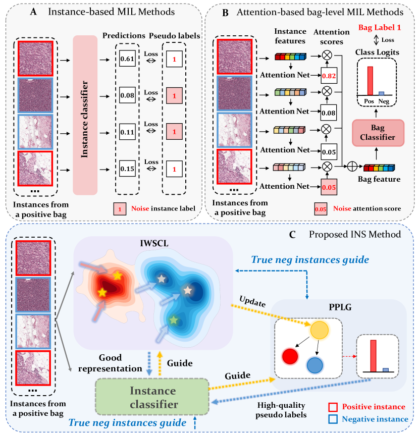
Figure 1: Motivation of our method. A. Existing instance-based MIL methods typically assign a bag’s label to its instances as pseudo labels, resulting in a large number of noises in instance pseudo labels. B. The loss function of bag-based MIL methods is defined at the bag level, which often only finds the most easily identifiable positive instances and ignores other more difficult ones. C. In contrast to these methods, we propose an effective instance-based MIL framework based on contrastive learning and prototype learning and a joint training strategy.

Currently, MIL methods for WSI classification can be divided into instance-based methods [13, 14, 11, 15] and bag-based methods [16, 17, 18, 19, 20, 21, 22, 23, 10, 24, 25]. Instance-based methods typically train an instance classifier with pseudo labels and then aggregate the predictions of instances to obtain the bag-level prediction. The main problem of this approach is that instance pseudo labels contain a lot of noise. Since the true label of each instance is unknown, the quality of the pseudo labels assigned to all instances is a key factor that determines the performance of this type of methods. However, existing studies usually assign instance pseudo labels by inheriting the label of the bag they belong to, which leads to a large amount of noise in the pseudo labels and greatly limits their performance. Figure 1 A shows the typical training process and issues of instance-based methods.

Bag-based methods first use an instance-level feature extractor to extract features for each instance in a bag, and then aggregate these features to obtain a bag-level feature, which is used to train a bag classifier. Most recent bag-based methods utilize attention mechanisms to aggregate instance features and they introduce an independent scoring module to generate learnable attention weights for each instance feature, which can be used to realize instance-level classification. Although this type of method overcomes the problem of noisy labels in instance-based methods, it also has the following issues: 1) Low performance in instance-level classification. We find that the difficulty of identifying different positive instances is different in the same positive bag (e.g., instances with larger tumor areas are easier to be identified than those with smaller tumor areas). Attention-based methods define losses at the bag level, which often leads to the result that only the most easily identifiable positive instances are found while other more difficult ones are missed [19, 12]. In other words, the network assigns higher attention weights to the most easily recognizable positive instances to achieve correct bag classification, without the need to find all positive instances, which greatly limits its instance-level classification performance. 2) Bag-level classification performance is not robust. As mentioned earlier, bag-level classification relies heavily on the attention scores assigned by the scoring network to each instance. When these attention scores are inaccurate, the performance of the bag classifier will also be affected. A typical example is the bias that occurs in classifying bags with a large number of difficult positive instances while very few easy positive instances. Figure 1 B shows the typical training process and issues of bag-based methods.

In the history of deep learning-based MIL research, although instance-based methods were first proposed, their reliance on instance pseudo labels, which are difficult to obtain, has led to a bottleneck in their performance. In contrast, an increasing number of researchers [20, 22] have focused on using stronger attention-based methods at the bag level to provide more accurate attention scores. However, intuitively, as long as the loss function is defined at the bag level, attention-based scoring methods will inevitably exhibit ”laziness” in finding more difficult positive instances [19, 12]. Different from the above-mentioned studies, we propose an instance-based MIL framework based on contrastive learning and prototype learning, called INS. Figure 1 C illustrates the main idea and basic components of INS. Our main objective is to directly train an efficient instance classifier at the fine-grained instance level, which needs to fulfill two requirements: first, obtaining a good instance-level feature representation, and second, assigning an accurate pseudo label to each instance. To this end, we propose instance-level weakly supervised contrastive learning (IWSCL) for the first time in the MIL setting to learn good instance representations, better separating negative and positive instances in the feature space. We also propose the Prototype-based Pseudo Label Generation (PPLG) strategy, which generates high-quality pseudo labels for each instance by maintaining two representative feature vectors as prototypes, one for negative instances and the other for positive instances. We further develop a joint training strategy for IWSCL, PPLG and the instance classifier. Overall, IWSCL and PPLG are completed under the guidance of the instance classifier’s predictions. At the same time, the good feature representations from IWSCL and the accurate pseudo labels from PPLG can then further improve the instance classifier. More importantly, we efficiently utilize the true negative instances from negative bags in the training set to guide all the instance classifier, the IWSCL and the PPLG, ensuring that INS iterates towards the right direction. After training the instance classifier, due to its strong instance classification performance, we can complete accurate bag classification using simple mean pooling.

We comprehensively evaluated the performance of INS on six tasks, using a simulated CIFAR10 dataset and three real-world datasets containing breast cancer, lung cancer, and cervical cancer. Extensive experimental results demonstrate that INS achieved better performance in both instance and bag classification than state-of-the-art methods. More importantly, our experiments not only include the tasks that human doctors can directly judge from H$\&$E-stained slides, like tumor diagnosis and tumor subtyping, but also the tasks that human doctors cannot directly make decisions from HE slides, including predicting lymph node metastasis from primary lesion, patient prognosis, and prediction of immunohistochemical markers. Given the strong instance-level classification ability of INS, we can use it for explainable research and new knowledge discovery in these difficult clinical tasks. In the task of predicting lymph node metastasis from primary lesion of cervical cancer, we use INS to classify high- and low-risk instances, thereby identifying the ”Micropapillae” pathological pattern that indicates high risk of lymph node metastasis.

The main contributions of this paper are as follows:

$\bullet$ We propose INS, an instance-based MIL framework that combines contrastive learning and prototype learning. This framework serves as an efficient instance classifier, capable of effectively addressing instance-level and bag-level classification tasks at the finest-grained instance level.

$\bullet$ We propose instance-level weakly supervised contrastive learning (IWSCL) for the first time in the MIL setting to learn good feature representations for each instance. We also propose the Prototype-based Pseudo Label Generation (PPLG) strategy, which generates high-quality pseudo labels for each instance through prototype learning. We further propose a joint training strategy for IWSCL, PPLG, and the instance classifier.

$\bullet$ We comprehensively evaluated the performance of INS on six tasks of four datasets. Extensive experiments and visualization results demonstrate that INS achieves the best performance of instance and bag classification.

2 Related Work

2.1 Instance-based MIL Methods

Instance-based methods train an instance classifier by assigning pseudo labels to each instance, and bag classification is achieved by aggregating the prediction of all instances in a bag. Early methods [26, 27, 28, 29] typically assign a bag’s label to all its instances, leading to a large number of noisy labels in positive bags. Some recent methods [13, 14, 11] select key instances and only use them for training, thus reducing the impact of noise to some extent. In this paper, we present a strong instance classifier and we believe that a good instance classifier requires both good instance-level representation learning and accurate pseudo instance labels. To fulfill this goal, we propose for the first time the instance-level weakly supervised contrastive learning under the MIL setting, which achieves efficient instance feature representation. We also propose a prototype learning-based strategy to generate high-quality pseudo labels.

2.2 Bag-based MIL Methods

Bag-based methods first extract instance features and then aggregate these features in a bag to generate bag features for training a bag classifier. Attention-based methods [16, 17, 18, 19, 20, 21, 10] are the mainstream of this paradigm, which typically use an independent scoring network for each instance feature to produce learnable attention weights, which can also be used to generate instance predictions. The main problem of these methods is that they cannot accurately identify difficult positive instances, resulting in limited instance and bag classification performance. Recently, some studies [19, 12, 24] have added instance-level classification loss to bag-level losses, but the pseudo labels assigned to instances are still noisy. Some methods have also been proposed to accomplish WSI classification using reinforcement learning [30], graph learning [31, 32], and bayesian learning [33]. However, none of them can effectively fulfill the instance classification task. In contrast, we directly start from the finest instance-level and use weakly supervised contrastive learning and prototype learning to complete instance feature learning and pseudo-label updating, thereby addressing both instance and bag classification.

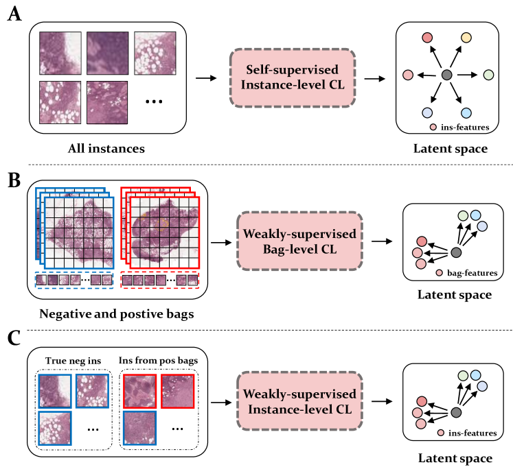
Figure 2: Comparison of our IWSCL with existing contrastive learning methods. The red box and blue box represent positive and negative instances, respectively. ”Ins” is the abbreviation for instances, ”pos” for positive, ”neg” for negative, and ”CL” for contrastive learning. A. Self-supervised instance-level contrastive learning separates instance features as much as possible, regardless of whether they are positive or negative. B. Weakly supervised contrastive learning at the bag level [25] does not take instance features into account. C. The proposed instance-level weakly supervised contrastive learning tries to separate positive and negative instances directly in the feature space.

2.3 Contrastive Learning for WSI Classification

Existing methods [20, 21, 22, 12, 34, 35, 36] usually first use WSI patches to pretrain an instance-level feature extractor through self-supervised learning and then perform model training using the extracted features. Most of them [20, 21, 12, 35, 36] use contrastive self-supervised learning methods [37, 38, 39] to extract instance features, but this process is completely unsupervised and it can only attempt to separate all instances as much as possible instead of effectively separating positive and negative instances. In the latest research, Wang et al. [25] proposed a feature-based contrastive learning method at the bag-level, but it still cannot perform effective instance classification. In contrast, we for the first time propose instance-level weakly supervised contrastive learning (IWSCL) under the MIL setting, which effectively separates negative and positive instance features. Figure 2 shows the differences between existing contrastive learning methods and our proposed IWSCL.

2.4 Prototype Learning for WSI Classification

Prototype learning, derived from Nearest Mean Classifiers, aims to provide a concise representation for instances. Recent studies demonstrate the potential of using representations or prototypes for classification, with variations in construction and utilization. PMIL [40] employs unsupervised clustering to construct prototypes, enhancing bag features by assessing instance similarity within bags. TPMIL [41] creates learnable prototype vectors, utilizing attention scores as soft pseudo-labels to assign instances. However, PMIL’s non-learnable prototypes focus on improving bag features, posing challenges for fine-grained instance classification. TPMIL heavily relies on attention scores, which often fail to accurately identify challenging positive instances. Additionally, their prototype learning lacks effective integration of feature-level contrastive learning, resulting in limited performance. In contrast, our proposed PPLG strategy generates high-quality pseudo-labels, utilizing joint training with instance contrastive representation learning, prototype learning, and the instance classifier. Our prototype learning also incorporates guidance from the instance classifier and includes true negative instances from negative bags in the training set.

3 Method

3.1 Problem Formulation

Given a dataset $X=\{X_{1},X_{2},\ldots,X_{N}\}$ containing $N$ WSIs, and each WSI $X_{i}$ is divided into non-overlapping patches $\{x_{i,j},j=1,2,\ldots n_{i}\}$, where $n_{i}$ denotes the number of patches obtained from $X_{i}$. All the patches from $X_{i}$ constitute a bag, where each patch is an instance of this bag. The label of the bag $Y_{i}\in\left\{0,1\right\},\ i=\{1,2,...N\}$, and the labels of each instance $\{y_{i,j},j=1,2,\ldots n_{i}\}$ have the following relationship:

$$Y_{i}=\left\{\begin{array}[]{cc}0,&\quad\text{ if }\sum_{j}y_{i,j}=0\\ 1,&\quad\text{ else }\end{array}\right.$$ (1)

This indicates that all instances in negative bags are negative, while in positive bags, there exists at least one positive instance. In the setting of weakly supervised MIL, only the labels of bags in the training set are available, while the labels of instances in positive bags are unknown. Our goal is to accurately predict the label of each bag (bag classification) and the label of each instance (instance classification) in the test set.

3.2 Framework Overview

Figure 3 presents the overall framework of the proposed INS, which aims to train an efficient instance classifier using instance-level weakly supervised contrastive learning (IWSCL) and Prototype-based Pseudo Label Generation (PPLG). We use the true negative instances from negative bags in the training set to guide all the instance classifier, the IWSCL and the PPLG, ensuring that INS iterates towards the right direction. IWSCL and PPLG are also guided by the instance classifier, and they also help improve the instance classifier through iterative optimization.

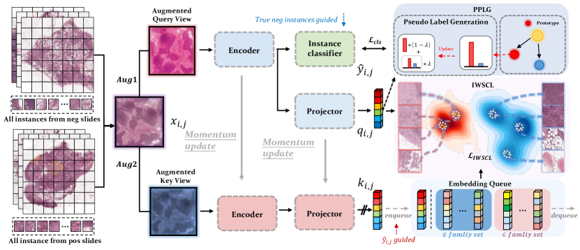
Figure 3: Workflow of the proposed INS framework, where ”pos” is the abbreviation for positive, ”neg” for negative, ”Aug” for augmentation, ”IWSCL” for the proposed instance-level weakly supervised contrastive learning, and ”PPLG” for the proposed prototype-based pseudo label generation.

Specifically, in one iteration, we first randomly select an instance $x_{i,j}$ from all instances in the training set, and generate a query view and a key view using two different augmentations. In the Query View branch, we input the query view into an Encoder and then feed its output to both the instance classifier and the MLP-based projector to obtain the predicted class ${\hat{y}}_{i,j}\in\mathbb{R}^{2}$ (a one-hot vector indicating negative or positive) and the feature embedding $q_{i,j}\in\mathbb{R}^{d}$, respectively. In the Key View branch, we input the key view into an Encoder and then feed its output to a Projector to obtain the feature embedding $k_{i,j}\in\mathbb{R}^{d}$, where both Encoder and Projector are updated through momentum-based methods from the Query View branch. Inspired by MOCO [38] and Pico [42], we maintain a large Embedding Queue to store the feature embeddings of the Key View branch together with the predicted class labels of the corresponding instances. Then, we use the current instance’s ${\hat{y}}_{i,j}$, $q_{i,j}$, $k_{i,j}$, and the Embedding Queue from the previous iteration to perform instance-level weakly supervised contrastive learning (IWSCL). For $q_{i,j}$, we pull closer the instance embeddings in the Embedding Queue that have the same predicted class and push away those with different predicted class. In the PPLG module, we maintain two representative feature vectors as prototypes for positive and negative classes during training. We use $q_{i,j}$ and the prototype vectors from the previous iteration to generate pseudo labels for $x_{i,j}$. Finally, we update the Embedding Queue using ${\hat{y}}_{i,j}$ and $k_{i,j}$, update the prototype vectors using ${\hat{y}}_{i,j}$ and $q_{i,j}$, and train the instance classifier with the generated pseudo label, which completes the current iteration. In addition, to prevent bag-level degradation during training, we add a bag-level constraint loss function. The IWSCL module and the PPLG module are presented in Section 3.3 and Section 3.4, respectively. The bag constraint and total loss are given in Section 3.5.

3.3 Instance-level Weakly Supervised Contrastive Learning

In contrastive learning, the most important step is to construct positive and negative sample sets, and then learn robust feature representations by pulling positive samples closer and pushing negative samples farther in the feature space [37, 38, 39]. To distinguish from the positive and negative instances in the MIL setting, we use family/non-family sample sets to represent the positive/negative sample sets in contrastive learning, respectively.

In traditional self-supervised contrastive learning, the standard method for constructing family and non-family sets is to use two augmented views of the same sample as family samples, while all other samples are considered as non-family sets. This can only force all samples to be as far away from each other as possible in the feature space, but cannot separate positive and negative instances in the MIL setting. In contrast, in the MIL setting, all instances from negative bags in the training set have true negative labels, and they naturally belong to the same set. This weak label information can effectively guide the instance-level contrastive learning, which is neglected in existing studies. We maintain a large Embedding Queue during training to store the feature embeddings $k_{i,j}$ of a large number of instances and their predicted classes ${\hat{y}}_{i,j}$ by the instance classifier. Note that for true negative instances, we no longer save their predicted classes, but directly assign them a definite negative class, i.e., ${\hat{y}}_{i,j}$=0.

Family and Non-family Sample Selection. For the instance $x_{i,j}$ and its embedding $q_{i,j}$, we use the instance classifier’s predicted class ${\hat{y}}_{i,j}$ and the Embedding Queue to construct its family set $F(q_{i,j})$ and non-family set $F^{\prime}(q_{i,j})$, and then perform contrastive learning based on $q_{i,j}$. Specifically, $F(q_{i,j})$ comes from two parts, of which the first part consists of the embeddings $q_{i,j}$ and $k_{i,j}$ and the second part consists of all embeddings in the Embedding Queue whose class label equals ${\hat{y}}_{i,j}$. Embeddings with the other class label in the Embedding Queue form the non-family set $F^{\prime}(q_{i,j})$.

Mathematically, for a given mini-batch, let all query and key embeddings be denoted as $B_{q}$ and $B_{k}$, and the Embedding Queue as $Q$. For an instance $(x_{i,j},q_{i,j},{\hat{y}}_{i,j})$, its contrastive embedding pool is defined as:

$$P\left(q_{i,j}\right)=\left(B_{q}\cup B_{k}\cup Q\right)\backslash\left\{q_{i,j}\right\}$$ (2)

In $P(q_{i,j})$, its family set $F(q_{i,j})$ and non-family set $F^{\prime}(q_{i,j})$ are defined as:

$$F\left(q_{i,j}\right)=\left\{m\mid m\in P\left(q_{i,j}\right),\hat{y}_{m}=\hat{y}_{i,j}\right\}$$ (3)

$$F^{\prime}\left(q_{i,j}\right)=P\left(q_{i,j}\right)\backslash F\left(q_{i,j}\right)$$ (4)

Contrastive Loss. We construct a contrastive learning loss based on the embedding $q_{i,j}$:

$$\mathcal{L}_{\mathit{IWSCL}}\left(q_{i,j}\right)=$$ (5)

$$-\frac{1}{\left|F\left(q_{i,j}\right)\right|}\sum_{{k}_{+}\in F\left(q_{i,j}\right)}\log\frac{\exp\left(q_{i,j}{}^{\top}{k}_{+}/\tau\right)}{\Sigma_{{k}^{-}\in F^{\prime}\left(q_{i,j}\right)}\exp\left(q_{i,j}{}^{\top}{k}_{-}/\tau\right)},$$

where ${k}_{+}$ denotes the family sample of the current $q_{i,j}$, ${k}_{-}$ denotes the non-family sample of the current $q_{i,j}$, and $\tau\geq 0$ is the temperature coefficient.

Embedding Queue Updating. At the end of each iteration, the current instance’s momentum embedding $k_{i,j}$ and its predicted label ${\hat{y}}_{i,j}$ or true negative label are added to the Embedding Queue, and the oldest embedding and its label are dequeued.

3.4 Prototype-based Pseudo Label Generation

On the basis of obtaining a meaningful feature representation, we assign more accurate pseudo labels to instances by prototype learning. To this end, we maintain two representative feature vectors, one for negative instances and the other for positive instances, as prototype vectors ${\mu}_{r}\in\mathbb{R}^{d},{r=0,1}$. The generation of pseudo labels and the updating process of prototypes are also guided by true negative instances and the instance classifier. If the current instance $x_{i,j}$ comes from a positive bag, we use its embedding $q_{i,j}$ and the prototype vectors ${\mu}_{r}$ to generate its pseudo label $s_{i,j}\in\mathbb{R}^{2}$. At the same time, we update the prototype vector of the corresponding class using its predicted label ${\hat{y}}_{i,j}$ and embedding $q_{i,j}$. If the current instance $x_{i,j}$ comes from a negative bag, we directly assign it a negative label and update the negative prototype vector using its embedding $q_{i,j}$. Then, we use the generated pseudo labels to train the instance classifier and complete this iteration.

Pseudo Label Generation. If the current instance $x_{i,j}$ comes from a positive bag, we calculate the inner product between its embedding $q_{i,j}$ and the two prototype vectors ${\mu}_{r}$, and select the prototype label with the smaller feature distance as the update direction $z_{i,j}\in\mathbb{R}^{2}$ for the pseudo label of $x_{i,j}$. Then, we use a moving updating strategy to update the pseudo label of the instance, defined as follows:

$$s_{i,j}=\alpha s_{i,j}+(1-\alpha)z_{i,j},z_{i,j}=onehot\left(\operatorname{argmax}q_{i,j}{}^{\top}{\mu}_{r}\right),$$ (6)

where $\alpha$ is a coefficient for moving updating, and $onehot(\cdot)$ is a function that converts a value to a two-dimensional one-hot vector. The moving updating strategy can make the process of updating pseudo labels smoother and more stable.

Prototype Updating. If the current instance $x_{i,j}$ comes from a positive bag, we update the corresponding prototype vector ${\mu}_{c}$ according to its predicted category ${\hat{y}}_{i,j}$ and embedding $q_{i,j}$ using a moving updating strategy as follows:

$${\mu}_{c}=\mathit{Norm}\left(\beta{\mu}_{c}+(1-\beta)q_{i,j}\right),c=\operatorname{argmax}\hat{y}_{i,j},$$ (7)

where $\beta$ is a coefficient for moving updating and $\mathit{Norm}(\cdot)$ is the normalization function.

If the current instance $x_{i,j}$ comes from a negative bag, i.e., $x_{i,j}$ is a true negative instance, we update the negative prototype vector ${\mu}_{0}$ using its embedding $q_{i,j}$ as follows:

$${\mu}_{0}=\mathit{Norm}\left(\beta{\mu}_{0}+(1-\beta)q_{i,j}\right)$$ (8)

Instance Classification Loss. We use the cross-entropy loss between the predicted value $p_{i,j}\in\mathbb{R}^{2}$ of the instance classifier and the pseudo label $s_{i,j}$ to train the instance classifier.

$$\mathcal{L}_{cls}=\mathit{CE}\left(p_{i,j},s_{i,j}\right),$$ (9)

where $\mathit{CE}(\cdot)$ represents the cross-entropy loss function.

3.5 Bag Constraint and Total Loss

Bag Constraint. To further utilize the bag labels, we record the bag index of each instance and apply the following bag constraint loss:

$$\mathcal{L}_{bc}=\mathit{CE}\left(\mathit{MLP}\left({Mean}\left(q_{i,j},j=1,2,\ldots n_{i}\right)\right),Y_{i}\right),$$ (10)

where $Mean(q_{i,j},j=1,2,\ldots n_{i})$ represents the mean pooling of all instance embeddings in a bag to obtain a bag embedding.

Total Loss. The total loss $\mathcal{L}$ is composed of the contrastive loss $\mathcal{L}_{\mathit{IWSCL\ }}$, instance classification loss $\mathcal{L}_{cls}$, and bag constraint loss $\mathcal{L}_{bc}$, defined as follows:

$$\mathcal{L}=\mathcal{L}_{\mathit{IWSCL}}+\lambda_{1}\mathcal{L}_{cls}+\lambda_{2}\mathcal{L}_{bc},$$ (11)

where $\lambda_{1}$ and $\lambda_{2}$ are weight coefficients used for balancing.

4 Experimental Results

4.1 Datasets

We used four datasets to comprehensively evaluate the instance and bag classification performance of INS, including a simulated dataset called CIFAR-MIL, constructed using CIFAR 10 [13], as well as three real WSI datasets: the Camelyon 16 Dataset [11] for breast cancer, the TCGA-Lung Cancer Dataset, and an in-house Cervical Cancer Dataset. More importantly, our experiments not only include the tasks that doctors can directly judge from H&E stained slides, including tumor diagnosis (on the Camelyon 16 Dataset) and tumor subtyping (on the TCGA-Lung Cancer Dataset), but also the tasks that doctors cannot directly make decisions from HE slides, including lymph node metastasis from primary lesion, patient prognosis, and prediction of immunohistochemical marker (all on the Cervical Cancer Dataset).

4.1.1 Simulated CIFAR-MIL Dataset

To evaluate the performance of INS under different positive ratios and compare it with the comparison methods, following WENO [14], we used 10-class natural image datasets CIFAR-10 [13] to construct a simulated WSI dataset called CIFAR-MIL with different positive ratios.

The CIFAR-10 dataset consists of 60,000 32$\times$32-pixel color images divided into 10 categories (airplane, automobile, bird, cat, deer, dog, frog, horse, ship, truck), with each category containing 6,000 images. Out of these images, 50,000 are used for training and 10,000 for testing. To simulate pathological Whole Slide Images (WSIs), we combined a set of random images from each category of the CIFAR-10 dataset to construct the WSI. Specifically, we treated each image from each category of the CIFAR-10 dataset as an instance, and only all instances of the ”truck” category were labeled as positive while the other instances were labeled as negative (the truck category is chosen at random). Then, we randomly selected a positive bag consisting of a set of $a$ positive instances and $100-a$ negative instances (without repetition) from all instances, with a positive ratio of $\frac{a}{100}$. Similarly, we randomly selected a negative bag consisting of 100 negative instances (without repetition). We repeated this process until all positive or negative instances in the CIFAR-10 dataset were used up. By adjusting the value of a, we constructed 5 subsets of the CIFAR-MIL dataset with positive ratios of 5%, 10%, 20%, 50%, and 70%, respectively.

4.1.2 Camelyon16 Public Dataset

The Camelyon16 dataset is a publicly available dataset of histopathology images used for detecting breast cancer metastasis in lymph nodes [11]. WSIs containing metastasis are labeled positive, while those without metastasis are labeled negative. In addition to slide-level labels indicating whether a WSI is positive or negative, the dataset also provides pixel-level labels for metastasis areas. To satisfy weakly supervised scenarios, we used only slide-level labels for training and evaluated the instance classification performance of each algorithm using the pixel-level labels of cancer areas. Prior to training, we divided each WSI into non-overlapping 512$\times$512 image patches under 10$\times$ magnification. Patches with entropy less than 5 were removed as background, and a patch was labeled positive if it contained 25% or more cancer areas, otherwise, it was labeled negative. A total of 186,604 instances were obtained for training and testing, with 243 slides used for training and 111 for testing.

4.1.3 TCGA Lung Cancer Dataset

The TCGA Lung Cancer dataset comprises 1054 WSIs obtained from the Cancer Genome Atlas (TCGA) Data Portal, which consists of two lung cancer subtypes, namely Lung Adenocarcinoma and Lung Squamous Cell Carcinoma. Our objective is to accurately diagnose both subtypes, with WSIs of Lung Adenocarcinoma labeled as negative and WSIs of Lung Squamous Cell Carcinoma labeled as positive. This dataset provides only slide-level labels and patch-level labels are unavailable. The dataset contains about 5.2 million patches at 20$\times$ magnification, with an average of approximately 5,000 patches per slide. These WSIs were randomly partitioned into 840 training slides and 210 test slides (4 low-quality corrupted slides are discarded).

4.1.4 Cervical Cancer Dataset

The Cervical Cancer dataset is an in-house clinical pathology dataset that includes 374 H&E-stained WSIs of primary lesions of cervical cancer from different patients, after slide selection. We conducted all experiments at 5$\times$ magnification, and we divided each WSI into non-overlapping patches of size 224$\times$224 to form a bag. Background patches with entropy values less than 5 were discarded from the original WSI. For prediction of lymph node metastasis in primary tumors, we labeled the corresponding slides of patients who developed pelvic lymph node metastasis as positive (209 cases) and those who did not develop pelvic lymph node metastasis as negative (165 cases). We randomly divided the WSIs into a training set (300 cases) and a test set (74 cases). For prediction of patient survival prognosis, following Skrede et al. [28], we grouped all patients based on detailed follow-up records using the median as a cutoff, where those who did not experience cancer-related death within three years were labeled as negative (good prognosis) and those who did were labeled as positive (poor prognosis). Then, we randomly divided the WSIs into a training set (294 cases) and a test set (80 cases) according to the labels. For prediction of the immunohistochemical marker KI-67, following Liu et al. [29] and Feng et al. [16], we grouped all patients based on detailed KI-67 immunohistochemistry reports using the median as a cutoff, where KI-67 levels below 75 were labeled as negative and those above 75 were labeled as positive. Then, we randomly divided the WSIs into a training set (294 cases) and a test set (80 cases) according to the labels.

4.2 Evaluation Metrics and Comparison Methods

For both instance and bag classification, we used Area Under Curve (AUC) and Accuracy as evaluation metrics. Bag classification performance is evaluated on all datasets but instance-level classification performance is only evaluated on the CIFAR-MIL Dataset and the Camelyon 16 Dataset, since only these two datasets have instance labels. We compared our INS to 11 competitors, including three instance-based methods: MILRNN[13], Chi-MIL[14], and DGMIL[11], and eight bag-based methods: ABMIL[16], Loss-ABMIL[19], CLAM [10], DSMIL[20], TransMIL[22], DTFD-MIL[21], TPMIL [41] and WENO[12]. In accordance with DSMIL [26], we employed SimCLR [27] as the self-supervised approach to pre-extract patch features for all techniques. Regarding all comparative approaches, we replicated them using the published codes and conducted a grid search on the crucial hyperparameters across all methods. We cited the reported results from their papers under the same experimental settings.

4.3 Implementation Details

In line with DSMIL [26], we conducted pre-processing on WSI datasets such as patch cropping and background removal. For all datasets, the encoders are implemented using the ResNet18. The Instance classifier is implemented using MLP. The Projector is a 2-layer MLP and the Prototype vectors are 128 dimensions. No pre-training of the network parameters is performed. The SGD optimizer is used to optimize the network parameters with a learning rate of 0.01, momentum of 0.9 and the batch size is 64. The length of Embedding Queue is 8192. In order to smooth the training process, we empirically set up the warm-up epochs. After warm-up, we updated pseudo labels and gave true negative labels. The hyperparameter thresholds vary for each dataset, and we used grid search on the validation set to determine the optimal values. For more details, please refer to our codes, which will be available soon.

4.4 Results on the Synthetic Dataset CIFAR-MIL

We constructed the synthetic WSI datasets CIFAR-MIL with varying positive instance ratios to investigate the instance and bag classification performance of each method at different positive instance ratios. The results are shown in Table 1 and Table 2. It can be seen that INS achieved the best performance in both instance and bag classification tasks at all positive instance ratios. Most methods cannot work well in low positive instance ratios of 5% and 10%, for which the AUC of INS exceeds 0.94. At positive instance ratios above 20%, the performance of INS is comparable to that of fully supervised methods.

Another interesting phenomenon is that most methods have higher bag classification performance when the positive ratio is higher than 20%, but the instance classification performance is still fairly poor. This suggests that accurately identifying all positive instances is not necessary to complete correct bag classification. As the positive ratio increases, there are many positive instances in positive bags, which makes the bag classification task easier. The network often only needs to identify the simplest positive instances to complete bag classification, losing the motivation to accurately classify all positive instances. In contrast, INS maintains high instance and bag classification performance at all positive instance ratios.

Table 1: Instance classification results on the CIFAR-MIL Dataset.

Positive instance ratio	5%	10%	20%	50%	70%
Fully supervised	0.9621	0.9723	0.9740	0.9699	0.9715
ABMIL (18’ICML)	0.8485	0.8505	0.8909	0.8224	0.7935
Loss-ABMIL (20’AAAI)	0.6915	0.7372	0.7430	0.7475	0.6881
Chi-MIL (20’MICCAI)	0.5872	0.6801	0.7039	0.6851	0.7091
DSMIL (21’CVPR)	0.5515	0.4918	0.8258	0.6152	0.7525
DGMIL (22’MICCAI)	0.7016	0.7818	0.8815	0.8217	0.8308
WENO (22’NeurIPS)	0.9408	0.9179	0.9657	0.9393	0.9525
INS (ours)	0.9418	0.9466	0.9668	0.9702	0.9720

Table 2: Bag classification results on the CIFAR-MIL Dataset.

Positive instance ratio	5%	10%	20%	50%	70%
Fully supervised	0.9621	0.9723	0.9740	0.9699	0.9715
ABMIL (18’ICML)	0.6783	0.9344	0.9678	1.0000	1.0000
Loss-ABMIL (20’AAAI)	0.4913	0.9108	0.9352	0.9475	1.0000
Chi-MIL (20’MICCAI)	0.5630	0.4519	0.8633	0.9105	1.0000
DSMIL(21’CVPR)	0.5174	0.5265	0.9468	0.9850	1.0000
DGMIL (22’MICCAI)	0.7159	0.9414	0.9681	0.9838	1.0000
WENO (22’NeurIPS)	0.9367	0.9900	1.0000	1.0000	1.0000
INS (ours)	0.9408	0.9903	1.0000	1.0000	1.0000

Table 3: Results on the Camelyon 16 Dataset.

	Instance-level		Bag-level
Methods	AUC	Accuracy	AUC	Accuracy
ABMIL (18’ICML)	0.8480	0.8033	0.8379	0.8198
MILRNN (19’Nat. Med)	0.8568	0.8174	0.8262	0.8198
Loss-ABMIL (20’AAAI)	0.8995	0.8512	0.8299	0.8018
Chi-MIL (20’MICCAI)	0.7880	0.7453	0.8256	0.8018
DSMIL (21’CVPR)	0.8858	0.8566	0.8401	0.8108
TransMIL (21’NeurIPS)	-	-	0.8566	0.8288
CLAM (21’ Nat. Biomed. Eng.)	0.8913	0.8655	0.8594	0.8378
DTFD-MIL (22’CVPR)	0.8928	0.8701	0.8638	0.8468
DGMIL (22’MICCAI)	0.9012	0.8859	0.8368	0.8018
WENO (22’NeurIPS)	0.9377	0.9057	0.8495	0.8108
TPMIL (23’MIDL)	0.9234	0.8867	0.8421	0.8018
INS (ours)	0.9583	0.9249	0.9016	0.8739

Table 4: Results on the TCGA-Lung Cancer Dataset.

	Bag-level
Methods	AUC	Accuracy
ABMIL (18’ICML)	0.9488	0.9000
MILRNN (19’Nat. Med)	0.9107	0.8619
Loss-ABMIL (20’AAAI)	0.9517	0.9143
Chi-MIL (20’MICCAI)	0.9523	0.9190
DSMIL(21’CVPR)	0.9633	0.9190
TransMIL(21’NeurIPS)	0.9830	0.9381
CLAM (21’Nat. Biomed. Eng.)	0.9788	0.9286
DTFD-MIL(22’CVPR)	0.9808	0.9524
DGMIL (22’MICCAI)	0.9702	0.9190
WENO (22’NeurIPS)	0.9727	0.9238
TPMIL (23’MIDL)	0.9799	0.9429
INS (ours)	0.9837	0.9571

Table 5: Results on the Cervical Cancer Dataset.

Clinical Tasks (Bag level)	Lymph node metastasis		Survival Prognosis		KI-67 Prediction
Methods	AUC	Accuracy	AUC	Accuracy	AUC	Accuracy
ABMIL (18’ICML)	0.7716	0.7297	0.7439	0.7125	0.6963	0.6500
Loss-ABMIL (20’AAAI)	0.7835	0.7568	0.7505	0.7250	0.6987	0.6625
Chi-MIL (20’MICCAI)	0.7783	0.7432	0.7349	0.7000	0.6933	0.6625
DSMIL (21’CVPR)	0.8022	0.7838	0.7622	0.7375	0.7124	0.6875
TransMIL (21’NeurIPS)	0.8126	0.7838	0.7716	0.7375	0.7252	0.6875
CLAM (21’Nat. Biomed. Eng.)	0.8138	0.7838	0.7755	0.7375	0.7297	0.7000
DTFD-MIL (22’CVPR)	0.8108	0.7703	0.7650	0.7375	0.7267	0.6875
DGMIL (22’MICCAI)	0.8056	0.7568	0.7515	0.7250	0.7115	0.6875
WENO (22’NeurIPS)	0.8222	0.7703	0.7775	0.7500	0.7323	0.7000
TPMIL (23’MIDL)	0.8213	0.7703	0.7728	0.7500	0.7318	0.7000
INS (ours)	0.8677	0.8243	0.7812	0.7625	0.7534	0.7125

4.5 Results on Real-World Datasets

4.5.1 Camelyon 16 Dataset

Table 3 shows the classification performance of INS and other methods on the Camelyon 16 Dataset. The low positive ratio of Camelyon 16 Dataset (about 10%-20%) makes the classification task quite difficult. INS outperforms all the compared methods with a large margin, exceeding the second-best method by 2.1% and 3.8% in AUC for instance and bag classification, respectively. Figure 4 shows typical visualization results on this dataset. It can be seen that INS accurately localizes almost all positive instances in the positive bags.

4.5.2 TCGA-Lung Cancer Dataset

Table 4 shows the results on the TCGA-Lung Cancer Dataset. Unlike the Camelyon 16 Dataset, this dataset has a high positive instance ratio (more than 80%), so the performance of all methods is fairly good, while INS still achieves the best performance.

4.5.3 Cervical Cancer Dataset

Table 5 shows the experimental results of three tasks on the in-house Cervical Cancer Dataset, including lymph node metastasis prediction from primary lesion, patient prognosis, and immunohistochemical marker KI-67 prediction from H&E stained WSIs. Unlike the previous two real-world datasets, these three tasks are very tough even for human doctors. It can be seen that INS significantly outperforms other methods in all three tasks, demonstrating the strong performance of INS.

Figure 4: Typical visualization results on the Camelyon 16 Dataset, where the yellow line represents the true tumor boundary annotated by doctors, and the pick boxes represent the positive instances predicted by INS as heatmaps.

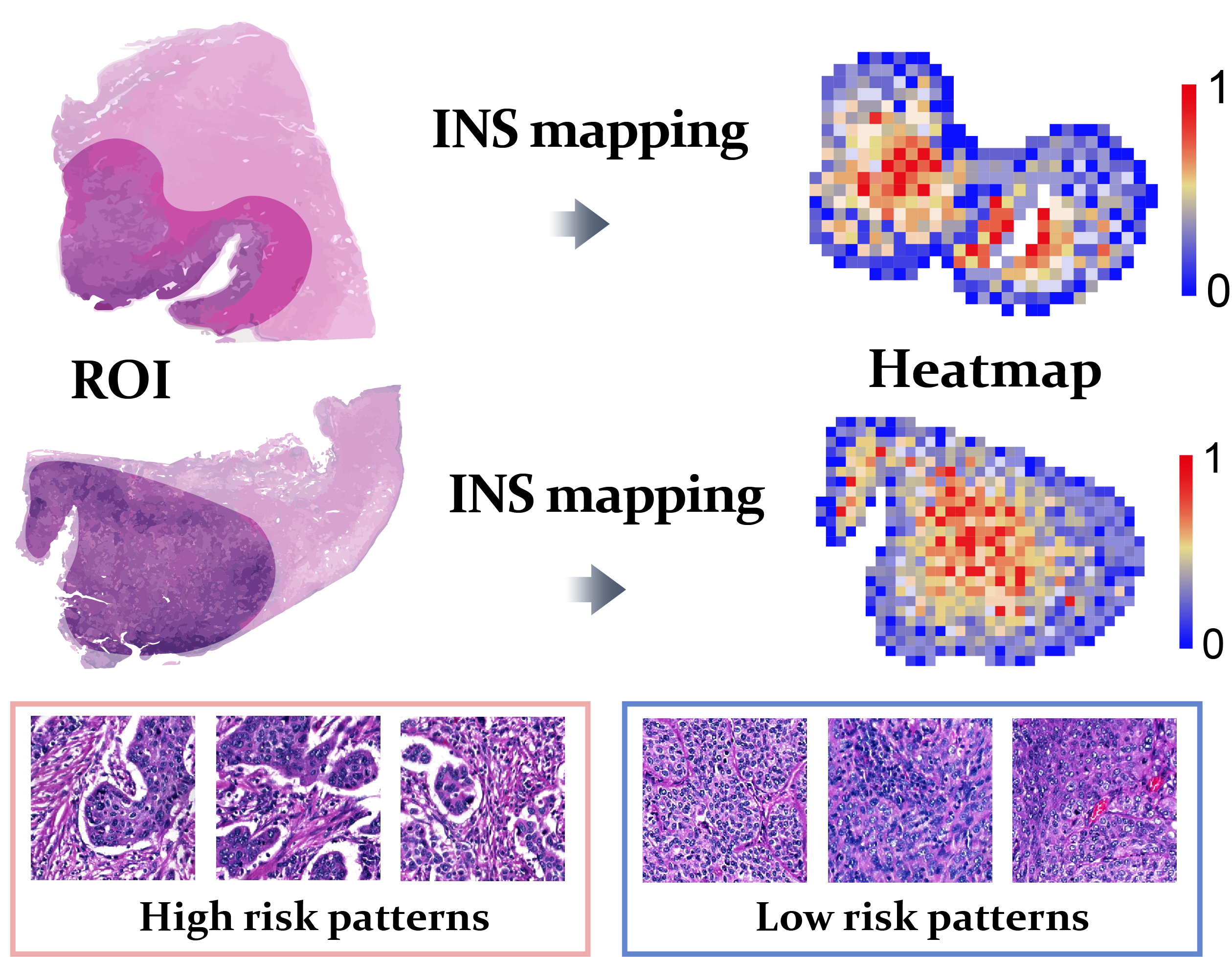
Figure 5: Heatmap visualization of INS on the lymph node metastasis task, where we identify the ”Micropapillae” pathological pattern that indicates positive metastasis from HE slides.

4.6 Interpretability Study of the Lymph Node Metastasis Task

As can be seen from Table 5, INS can predict the preoperative lymph node status of cervical cancer with high performance using HE-stained slides of the primary tumor. However, this does not offer pathologists additional interpretable pathological patterns. While cancer diagnosis is possible through visual inspection of HE-stained pathological slides, the same cannot be said for accurately determining lymph node metastasis status from the primary lesion. Given INS’s powerful instance classification ability, we hope to find explicit pathological patterns that can suggest the lymph node metastasis status and perform interpretable analysis as well as new knowledge discovery. Specifically, we used INS to predict the probability of each instance being positive within the positive bags, and visualized the top 0.1% instances with the highest and lowest probabilities separately. These instances with the highest predicted positive probabilities are likely to contain pathological patterns that identify high-risk lymph node metastasis, as shown in Figure 5.

As can be seen, in images suggesting lymph node metastasis, structures resembling ”micropapillae” are more prevalent, indicating a high-risk pathological pattern. Micropapillary structures are characterized by small clusters of infiltrating cancer cells forming hollow or mulberry-like nests without a central fibrovascular axis, surrounded by blank lacunae or lacunae between interstitial components. Conversely, negative lymph node images more commonly exhibit a ”sheet-like” pattern, in which cells form tightly connected nests of varying sizes within the tumor interstitium, with fissures or lacunae rarely observed. This conclusion highlights the interpretability of using INS to assess lymph node metastasis and its significant guiding implications for future clinical research.

5 Ablation Study and Further Analysis

5.1 Ablation Study on Key Components

We conducted comprehensive ablation experiments on the components of INS using the Camelyon 16 Dataset, and the results are shown in Table 6. Here, w/o $\mathcal{L}_{\mathit{IWSCL\ }}$ means that weakly supervised contrastive learning is not used, w/o $\mathcal{L}_{bc}$ means that bag-level constraint is not used, and w/o MU means that $\alpha$=0 in formula 4, indicating that the pseudo label updating strategy with moving updating is not used. It can be seen that IWSCL is the crucial component of INS, and without contrastive learning, the performance of INS declines significantly. Both the bag constraint and the pseudo label updating strategy with moving updating can effectively improve the performance of INS. It is worth noting that INS still outperforms all comparing methods even without either one of these two components.

Table 6: Results of ablation study on the Camelyon 16 Dataset.

Conditions	$\mathcal{L}_{\mathit{IWSCL}}$	$\mathcal{L}_{bc}$	pseudo label	Instance AUC	Bag AUC
Ours	✓	✓	✓	0.9583	0.9016
w/o $\mathcal{L}_{\mathit{IWSCL}}$		✓	✓	0.9005	0.8301
w/o $\mathcal{L}_{bc}$	✓		✓	0.9411	0.8734
w/o MU	✓	✓	✓	0.9423	0.8815

5.2 Further Analysis

We conducted more detailed evaluation and interpretive experiments of INS.

Effective Representation Learning of INS. Currently, many studies [20, 21, 22, 12, 34, 35] use pre-trained feature extractors to extract instance features for subsequent training, among which ImageNet pretrained method [22] and contrastive self-supervised methods [20, 21, 12, 35, 36] are most commonly used. We compared these feature extraction methods with INS on the Camelyon16 Dataset. Specifically, we first used feature extractors pre-trained by ImageNet [43], SimCLR [37], DGMIL [11], and our INS, respectively, to extract all instance features. All methods used ResNet-18 as the network structure. Then we used the true labels of each instance only based on these features to train a simple SVM classifier and a linear classifier and tested the two classifiers on the test set to evaluate these features. Please note that the pre-training process of feature extractors is unsupervised (not using labels) or weakly supervised (using only bag labels), while the process of training SVM and Linear with the pre-extracted features is fully supervised using instance labels, enabling an effective evaluation of the quality of the pre-extracted features. We also trained the network in an end-to-end way as an upper bound. The results are shown in Figure 6 A. The features extracted from INS achieve the best results, indicating effectiveness of our method.

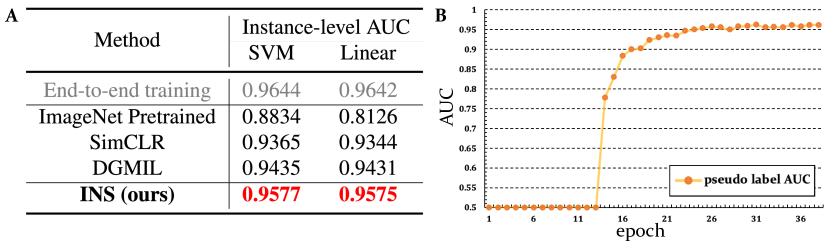
Figure 6: A. SVM and linear evaluation of pre-extracted features on the Camelyon16 Dataset. B. Visualization of the quality assessment of generated pseudo labels.

In addition, we use SimCLR and our INS to extract features of all instances from a typical slide in the Camelyon16 Dataset and visualize the feature distribution using t-SNE, as shown in Figure 7. It can be visually observed that the positive and negative instances are separated in the features extracted by INS. Surprisingly, we can even manually draw a clear boundary between them on the two-dimensional plane, indicating the powerful feature representation ability of INS. In contrast, although the features of SimCLR are relatively scattered in the feature space, there is significant overlapping between the positive and negative instances, which cannot be easily separated.

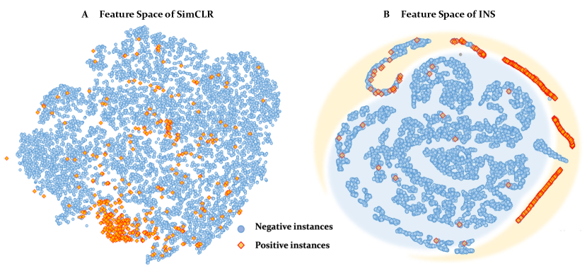
Figure 7: Visualization of feature distribution on a typical slide on the Camelyon16 Dataset using t-SNE. A. Instance features extracted by SimCLR. B. Instance features extracted by our INS.

Evaluation of Pseudo Labels. To intuitively demonstrate the quality of the instance pseudo labels, we plotted the AUC curve of the pseudo labels for all instances in the training set of the CIFAR-MIL Dataset (with a 0.2 positive instance ratio) against the training epochs, as shown in Figure 6 B. It can be clearly seen that the quality of the pseudo labels continues to improve, providing more and more effective guidance to the instance classifier.

6 Conclusion

In this paper, we propose INS, an instance-level MIL framework based on contrastive learning and prototype learning, which effectively addresses both instance and bag classification tasks. Guided by true negative instances, we propose a weakly-supervised contrastive learning method for effective instance-level feature representation under the MIL setting. In addition, we propose a prototype-based pseudo label generation method that generates high-quality pseudo labels for instances from positive bags. We further propose a joint training strategy for weakly-supervised contrastive learning, prototype learning, and instance classification. Extensive experiments on one synthetic dataset and five tasks on three real datasets demonstrate the strong performance of INS. With only slide labels, INS has the ability to accurately locate positive instances and has the potential to discover new knowledge or perform interpretability research on tough clinical tasks.

References

- [1] L. Qu, S. Liu, X. Liu, M. Wang, and Z. Song, “Towards label-efficient automatic diagnosis and analysis: a comprehensive survey of advanced deep learning-based weakly-supervised, semi-supervised and self-supervised techniques in histopathological image analysis,” Phys. Med. Biol., 2022.
- [2] C. L. Srinidhi, O. Ciga, and A. L. Martel, “Deep neural network models for computational histopathology: A survey,” Med. Image Anal., vol. 67, p. 101813, 2021.
- [3] M. Y. Lu, T. Y. Chen, D. F. Williamson, M. Zhao, M. Shady, J. Lipkova, and F. Mahmood, “Ai-based pathology predicts origins for cancers of unknown primary,” Nature, vol. 594, no. 7861, pp. 106–110, 2021.
- [4] F. Mahmood, D. Borders, R. J. Chen, G. N. McKay, K. J. Salimian, A. Baras, and N. J. Durr, “Deep adversarial training for multi-organ nuclei segmentation in histopathology images,” IEEE Trans. Med. Imaging, vol. 39, no. 11, pp. 3257–3267, 2019.
- [5] M. Y. Lu, R. J. Chen, D. Kong, J. Lipkova, R. Singh, D. F. Williamson, T. Y. Chen, and F. Mahmood, “Federated learning for computational pathology on gigapixel whole slide images,” Med. Image Anal., vol. 76, p. 102298, 2022.
- [6] J. Rony, S. Belharbi, J. Dolz, I. B. Ayed, L. McCaffrey, and E. Granger, “Deep weakly-supervised learning methods for classification and localization in histology images: a survey,” arXiv:1909.03354, 2019.
- [7] V. Cheplygina, M. de Bruijne, and J. P. Pluim, “Not-so-supervised: a survey of semi-supervised, multi-instance, and transfer learning in medical image analysis,” Med. Image Anal., vol. 54, pp. 280–296, 2019.
- [8] R. J. Chen, M. Y. Lu, J. Wang, D. F. Williamson, S. J. Rodig, N. I. Lindeman, and F. Mahmood, “Pathomic fusion: an integrated framework for fusing histopathology and genomic features for cancer diagnosis and prognosis,” IEEE Trans. Med. Imaging, vol. 41, no. 4, pp. 757–770, 2020.
- [9] M. Y. Lu, R. J. Chen, J. Wang, D. Dillon, and F. Mahmood, “Semi-supervised histology classification using deep multiple instance learning and contrastive predictive coding,” arXiv:1910.10825, 2019.
- [10] M. Y. Lu, D. F. Williamson, T. Y. Chen, R. J. Chen, M. Barbieri, and F. Mahmood, “Data-efficient and weakly supervised computational pathology on whole-slide images,” Nat. Biomed. Eng., vol. 5, no. 6, pp. 555–570, 2021.
- [11] L. Qu, X. Luo, S. Liu, M. Wang, and Z. Song, “Dgmil: Distribution guided multiple instance learning for whole slide image classification,” in MICCAI. Springer, 2022, pp. 24–34.
- [12] L. Qu, M. Wang, Z. Song et al., “Bi-directional weakly supervised knowledge distillation for whole slide image classification,” NeurIPS, vol. 35, pp. 15 368–15 381, 2022.
- [13] G. Campanella, M. G. Hanna, L. Geneslaw, A. Miraflor, V. Werneck Krauss Silva, K. J. Busam, E. Brogi, V. E. Reuter, D. S. Klimstra, and T. J. Fuchs, “Clinical-grade computational pathology using weakly supervised deep learning on whole slide images,” Nat. Med., vol. 25, no. 8, pp. 1301–1309, 2019.
- [14] P. Chikontwe, M. Kim, S. J. Nam, H. Go, and S. H. Park, “Multiple instance learning with center embeddings for histopathology classification,” in MICCAI. Springer, 2020, pp. 519–528.
- [15] F. Kanavati, G. Toyokawa, S. Momosaki, M. Rambeau, Y. Kozuma, F. Shoji, K. Yamazaki, S. Takeo, O. Iizuka, and M. Tsuneki, “Weakly-supervised learning for lung carcinoma classification using deep learning,” Sci. Rep., vol. 10, no. 1, p. 9297, 2020.
- [16] M. Ilse, J. Tomczak, and M. Welling, “Attention-based deep multiple instance learning,” in ICML. PMLR, 2018, pp. 2127–2136.
- [17] N. Hashimoto, D. Fukushima, R. Koga, Y. Takagi, K. Ko, K. Kohno, M. Nakaguro, S. Nakamura, H. Hontani, and I. Takeuchi, “Multi-scale domain-adversarial multiple-instance cnn for cancer subtype classification with unannotated histopathological images,” in CVPR, 2020, pp. 3852–3861.
- [18] J. Yao, X. Zhu, J. Jonnagaddala, N. Hawkins, and J. Huang, “Whole slide images based cancer survival prediction using attention guided deep multiple instance learning networks,” Med. Image Anal., vol. 65, p. 101789, 2020.
- [19] X. Shi, F. Xing, Y. Xie, Z. Zhang, L. Cui, and L. Yang, “Loss-based attention for deep multiple instance learning,” in AAAI, vol. 34, no. 04, 2020, pp. 5742–5749.
- [20] B. Li, Y. Li, and K. W. Eliceiri, “Dual-stream multiple instance learning network for whole slide image classification with self-supervised contrastive learning,” in CVPR, 2021, pp. 14 318–14 328.
- [21] H. Zhang, Y. Meng, Y. Zhao, Y. Qiao, X. Yang, S. E. Coupland, and Y. Zheng, “Dtfd-mil: Double-tier feature distillation multiple instance learning for histopathology whole slide image classification,” in CVPR, 2022, pp. 18 802–18 812.
- [22] Z. Shao, H. Bian, Y. Chen, Y. Wang, J. Zhang, X. Ji et al., “Transmil: Transformer based correlated multiple instance learning for whole slide image classification,” NeurIPS, vol. 34, pp. 2136–2147, 2021.
- [23] R. J. Chen, M. Y. Lu, W.-H. Weng, T. Y. Chen, D. F. Williamson, T. Manz, M. Shady, and F. Mahmood, “Multimodal co-attention transformer for survival prediction in gigapixel whole slide images,” in ICCV, 2021, pp. 4015–4025.
- [24] A. Myronenko, Z. Xu, D. Yang, H. R. Roth, and D. Xu, “Accounting for dependencies in deep learning based multiple instance learning for whole slide imaging,” in MICCAI. Springer, 2021, pp. 329–338.
- [25] X. Wang, J. Xiang, J. Zhang, S. Yang, Z. Yang, M.-H. Wang, J. Zhang, Y. Wei, J. Huang, and X. Han, “Scl-wc: Cross-slide contrastive learning for weakly-supervised whole-slide image classification,” in NeurIPS.
- [26] Y. Yan, X. Wang, X. Guo, J. Fang, W. Liu, and J. Huang, “Deep multi-instance learning with dynamic pooling,” in ACML. PMLR, 2018, pp. 662–677.
- [27] X. Wang, Y. Yan, P. Tang, X. Bai, and W. Liu, “Revisiting multiple instance neural networks,” Pattern Recognit., vol. 74, pp. 15–24, 2018.
- [28] O. Z. Kraus, J. L. Ba, and B. J. Frey, “Classifying and segmenting microscopy images with deep multiple instance learning,” Bioinformatics, vol. 32, no. 12, pp. i52–i59, 2016.
- [29] O. Maron and T. Lozano-Pérez, “A framework for multiple-instance learning,” NeurIPS, vol. 10, 1997.
- [30] Z. Zhu, L. Yu, W. Wu, R. Yu, D. Zhang, and L. Wang, “Murcl: Multi-instance reinforcement contrastive learning for whole slide image classification,” IEEE Trans. Med. Imaging, 2022.
- [31] Y. Zheng, R. H. Gindra, E. J. Green, E. J. Burks, M. Betke, J. E. Beane, and V. B. Kolachalama, “A graph-transformer for whole slide image classification,” IEEE Trans. Med. Imaging, vol. 41, no. 11, pp. 3003–3015, 2022.
- [32] W. Hou, C. Lin, L. Yu, J. Qin, R. Yu, and L. Wang, “Hybrid graph convolutional network with online masked autoencoder for robust multimodal cancer survival prediction,” IEEE Trans. Med. Imaging, 2023.
- [33] J.-G. Yu, Z. Wu, Y. Ming, S. Deng, Q. Wu, Z. Xiong, T. Yu, G.-S. Xia, Q. Jiang, and Y. Li, “Bayesian collaborative learning for whole-slide image classification,” IEEE Trans. Med. Imaging, 2023.
- [34] R. J. Chen, C. Chen, Y. Li, T. Y. Chen, A. D. Trister, R. G. Krishnan, and F. Mahmood, “Scaling vision transformers to gigapixel images via hierarchical self-supervised learning,” in CVPR, 2022, pp. 16 144–16 155.
- [35] R. J. Chen and R. G. Krishnan, “Self-supervised vision transformers learn visual concepts in histopathology,” arXiv:2203.00585, 2022.
- [36] H. Cai, X. Feng, R. Yin, Y. Zhao, L. Guo, X. Fan, and J. Liao, “Mist: multiple instance learning network based on swin transformer for whole slide image classification of colorectal adenomas,” J. Pathol., vol. 259, no. 2, pp. 125–135, 2023.
- [37] T. Chen, S. Kornblith, M. Norouzi, and G. Hinton, “A simple framework for contrastive learning of visual representations,” in ICML. PMLR, 2020, pp. 1597–1607.
- [38] K. He, H. Fan, Y. Wu, S. Xie, and R. Girshick, “Momentum contrast for unsupervised visual representation learning,” in CVPR, 2020, pp. 9729–9738.
- [39] M. Caron, H. Touvron, I. Misra, H. Jégou, J. Mairal, P. Bojanowski, and A. Joulin, “Emerging properties in self-supervised vision transformers,” in ICCV, 2021, pp. 9650–9660.
- [40] J.-G. Yu, Z. Wu, Y. Ming, S. Deng, Y. Li, C. Ou, C. He, B. Wang, P. Zhang, and Y. Wang, “Prototypical multiple instance learning for predicting lymph node metastasis of breast cancer from whole-slide pathological images,” Med. Image Anal., p. 102748, 2023.
- [41] L. Yang, D. Mehta, S. Liu, D. Mahapatra, A. Di Ieva, and Z. Ge, “Tpmil: Trainable prototype enhanced multiple instance learning for whole slide image classification,” arXiv:2305.00696, 2023.
- [42] H. Wang, R. Xiao, Y. Li, L. Feng, G. Niu, G. Chen, and J. Zhao, “Pico: Contrastive label disambiguation for partial label learning,” arXiv:2201.08984, 2022.
- [43] J. Deng, W. Dong, R. Socher, L.-J. Li, K. Li, and L. Fei-Fei, “Imagenet: A large-scale hierarchical image database,” in CVPR. IEEE, 2009, pp. 248–255.