$D$-Optimal Subsampling Design for Massive Data Linear Regression

Abstract.

Data reduction is a fundamental challenge of modern technology, where classical statistical methods are not applicable because of computational limitations. We consider linear regression for an extraordinarily large number of observations, but only a few covariates. Subsampling aims at the selection of a given percentage of the existing original data. Under distributional assumptions on the covariates, we derive $D$-optimal subsampling designs and study their theoretical properties. We make use of fundamental concepts of optimal design theory and an equivalence theorem from constrained convex optimization. The thus obtained subsampling designs provide simple rules for whether to accept or reject a data point, allowing for an easy algorithmic implementation. In addition, we propose a simplified subsampling method with lower computational complexity that differs from the $D$-optimal design. We present a simulation study, comparing both subsampling schemes with the IBOSS method in the case of a fixed size of the subsample.

1. Introduction

Data reduction is a fundamental challenge of modern technology, which allows us to collect huge amounts of data. Often, technological advances in computing power do not keep pace with the amount of data, creating a need for data reduction. We speak of big data whenever the full data size is too large to be handled by traditional statistical methods. We usually distinguish between the case where the number of covariates is large and the case where there are very many observations. The first case is referred to as high-dimensional data and numerous methods have been studied to deal with such data, most notably LASSO by Tibshirani (1996), which utilizes $\ell_{1}$ penalization to find sparse parameter vectors, thus fusing subset selection and ridge regression. We consider the second case, referred to as massive data. To deal with huge amounts of observations typically one of two methods is applied: One strategy is to divide the data into several smaller datasets and compute them separately, known as divide-and-conquer, see Lin and Xi (2011). Alternatively one can find an informative subsample of the full data. This can be done in a probabilistic fashion, creating random subsamples in a nonuniform manner. Among the prominent studies are Drineas et al. (2006), Mahoney (2011) and Ma et al. (2014). They present subsampling methods for linear regression models called algorithmic leveraging, which draw samples according to probabilities based on the normalized statistical leverage scores of the covariate matrix. More recently, Dereziński and Warmuth (2018) studied volume sampling, where subsamples are chosen proportional to the squared volume of the parallelepiped spanned by its observations. Conversely, subdata can be selected in a deterministic way. Shi and Tang (2021) present such a method, that maximizes the minimal distance between two observations in the subdata. Most prominently, Wang et al. (2019) have introduced the information-based optimal subdata selection (IBOSS) to tackle big data linear regression in a deterministic fashion based on $D$-optimality. The IBOSS approach selects the outer-most data points of each covariate successively. Other subsampling methods for linear regression include the works by Wang et al. (2021), who have introduced orthogonal subsampling inspired by orthogonal arrays, which selects observations in the corners of the design space and the optimal design based subsampling scheme by Deldossi and Tommasi (2021). Subsampling becomes increasingly popular, leading to more work outside linear models. Cheng et al. (2020) extent the idea of the IBOSS method from the linear model to logistic regression and other work on generalized linear regression include the papers by Zhang et al. (2021) and Ul Hassan and Miller (2019). Su et al. (2022) have recently considered subsampling for missing data, whereas Joseph and Mak (2021) focused on non-parametric models and make use of the information in the dependent variables. Various works consider subsampling when the full data is distributed over several data sources, among them Yu et al. (2022) and Zhang and Wang (2021) For a more thorough recent review on design inspired subsampling methods see the work by Yu et al. (2023).

In this paper we assume that both the model and the shape of the joint distribution of the covariates are known. We search for $D$-optimal continuous subsampling designs of total measure $\alpha$ that are bounded from above by the distribution of the covariates. Wynn (1977) and Fedorov (1989) were the first to study such directly bounded designs. Pronzato (2004) considered this setting using subsampling designs standardized to one and bounded by $1/\alpha$ times the distribution of the covariates. More recently, the same has been studied by Pronzato and Wang (2021) in the context of sequential subsampling. In Reuter and Schwabe (2023) we have studied bounded $D$-optimal subsampling designs for polynomial regression in one covariate, using many similar ideas as we use here. We stay with the unstandardized version emphasizing the subsampling character of the design. For the characterization of the optimal subsampling design, we will make use of an equivalence theorem from Sahm and Schwabe (2001). This equivalence theorem allows us to construct such subsampling designs for different settings of the distributional assumptions on the covariates. Based on this, we propose a simple subsampling scheme for selecting observations. This method includes all data points in the support of the optimal subsampling design and rejects all other observations. Although this approach is basically probabilistic, as it allows selection probabilities, the resulting optimal subsampling design is purely deterministic, since it depends only on the acceptance region defined by the optimal subsampling design. We make comments on the asymptotic behavior of the ordinary least squares estimator based on the $D$-optimal subsampling design that selects the data points with the largest Mahalanobis distance from the mean of the data.

Since the proposed algorithm requires computational complexity of the same magnitude as calculating the least squares estimator on the full data, we also propose a simplified version with lower computational complexity, that takes the variances of the covariates into account while disregarding the covariances between them.

The rest of this paper is organized as follows. After introducing the model in Section 2 we present the setup and establish necessary concepts and notation in Section 3. Section 3.1 illustrates our methodology for linear regression in one explanatory variable. We construct optimal subsampling designs for multiple linear regression in Section 3.2. In Section 4 we consider the case of a fixed subsample size, then examine the performance of our method in simulation studies in Section 5. We make concluding remarks in Section 6. Technical details and proofs are deferred to an Appendix.

2. Model Specification

We treat the situation of data $({\bf x}_{i},y_{i})$, where $y_{i}$ is the value of the response variable $Y_{i}$ and the ${\bf x}_{i}$ are realizations of the $d$-dimensional i.i.d. random vectors $\bm{X}_{i}$ of covariates with probability density function $f_{\bm{X}}$ for unit $i=1,\dots,n$. We assume the covariates $\bm{X}_{i}$ have an elliptical distribution. We suppose that the dependence of the response variable on the covariates $\bm{X}_{i}=(X_{i1},\dots,X_{id})^{\top}$ is given by the multiple linear regression model

$$Y_{i}=\beta_{0}+\beta_{1}X_{i1}+\beta_{2}X_{i2}+\dots+\beta_{d}X_{id}+\varepsilon_{i}$$

with independent, homoscedastic errors $\varepsilon_{i}$ with zero mean and $\operatorname{Var}[\varepsilon_{i}]=\sigma_{\varepsilon}^{2}<\infty$ which we assume to be independent of all $\bm{X}_{i^{\prime}}$.

We assume that the number of observations $n$ is very large. The aim is to estimate the regression parameter $\bm{\beta}=(\beta_{0},\dots,\beta_{d})^{\top}$, where $\beta_{0}$ is the intercept and $\beta_{j}$ is the slope parameter in the $j$-th component $x_{j}$ of ${\bf x}=(x_{1},\dots,x_{d})^{\top}$ for $j=1,\dots,d$. For notational convenience we write the multiple linear regression model as a general linear model

$$Y_{i}={\bf f}(\bm{X}_{i})^{\top}\bm{\beta}+\varepsilon_{i},\;\;\;i=1,\dots,n\,,$$

where ${\bf f}({\bf x})=(1,{\bf x}^{\top})^{\top}$.

3. Subsampling Design

We consider a scenario where the $y_{i}$ are expensive to observe and therefore only a percentage $\alpha$ ($0<\alpha<1$) of the $y_{i}$ are observed, given all ${\bf x}_{i}$. Another possible setting is that all $y_{i}$ and ${\bf x}_{i}$ are available, but parameter estimation is only computationally feasible on a percentage $\alpha$ of the data. Either setup leads to the question which subsample of the data $({\bf x}_{i},y_{i})$ yields the best estimation of the parameter $\bm{\beta}$ or essential parts of it.

Throughout this section we assume, that the distribution of $\bm{X}_{i}$ and its density $f_{\bm{X}}$ are known. We consider continuous designs $\xi$ with total measure $\alpha$ on $\mathbb{R}^{d}$ with density functions $f_{\xi}$ that are bounded from above by the density of the covariates $f_{\bm{X}}$ such that $\int f_{\xi}({\bf x})\mathop{}\!\mathrm{d}{\bf x}=\alpha$ and $f_{\xi}({\bf x})\leq f_{\bm{X}}({\bf x})$ for all ${\bf x}\in\mathbb{R}^{d}$. The resulting set of all such designs $\xi$ is denoted by $\Xi^{f_{\bm{X}}}$. A subsample can then be generated according to such a continuous design by accepting units $i$ with probability $f_{\xi}({\bf x}_{i})/f_{\bm{X}}({\bf x}_{i})$.

Let ${\bf M}(\xi)=\int{\bf f}({\bf x}){\bf f}({\bf x})^{\top}\xi(\mathop{}\!\mathrm{d}{\bf x})$ be the information matrix of $\xi$. We require $\operatorname{E}[\|\bm{X}_{i}\|^{2}_{2}]<\infty$ as some entries of the information matrix can be infinite otherwise. ${\bf M}(\xi)$ measures the quality of the least squares estimator $\hat{\bm{\beta}}$ based on a subsample according to $\xi$ in the sense that $\sqrt{\alpha n}(\hat{\bm{\beta}}-\bm{\beta})$ asymptotically follows a normal distribution with mean zero and covariance matrix $\sigma_{\varepsilon}^{2}{\bf M}(\xi)^{-1}$ when $n$ tends to infinity. To find an appropriate subsampling design $\xi\in\Xi^{f_{\bm{X}}}$, we aim to minimize the design criterion for $D$-optimality $\Psi(\xi)=-\ln(\det({\bf M}(\xi)))$. Then, the $D$-optimal design minimizes the determinant of the asymptotic covariance matrix of the parameter least squares estimator and can be interpreted as minimizing the volume of the respective confidence ellipsoid of $\bm{\beta}$. The optimal subsampling design that minimizes $\Psi(\xi)$ in $\Xi^{f_{\bm{X}}}$ is denoted by $\xi^{*}$ with density $f_{\xi^{*}}$. We make use of the sensitivity function $\psi({\bf x},\xi)=\alpha{\bf f}({\bf x})^{\top}{\bf M}(\xi)^{-1}{\bf f}({\bf x})$ (see Lemma A.1). For the characterization of the $D$-optimal continuous subsampling design, we apply the constrained equivalence theorem under Kuhn-Tucker conditions (see Sahm and Schwabe, 2001, Corollary 1 (c)) to the present case of multiple linear regression in the following theorem.

Theorem 3.1.

In multiple linear regression with $d\geq 2$ covariates with density $f_{\bm{X}}({\bf x})$ of the covariates $\bm{X}_{i}$, the subsampling design $\xi^{*}$ is $D$-optimal if and only if there exist a subset $\mathcal{X}^{*}\subset\mathbb{R}^{d}$ and a threshold $s^{*}$ such that

• $\xi^{*}$ has density $f_{\xi^{*}}({\bf x})=f_{\bm{X}}({\bf x})\mathds{1}_{\mathcal{X}^{*}}({\bf x})$

• $\psi({\bf x},\xi^{*})\geq s^{*}$ for ${\bf x}\in\mathcal{X}^{*}$, and

• $\psi({\bf x},\xi^{*})<s^{*}$ for ${\bf x}\not\in\mathcal{X}^{*}$.

Here, $\mathds{1}_{A}({\bf x})$ denotes the indicator function, i. e. $\mathds{1}_{A}({\bf x})=1$, if ${\bf x}\in A$ and $\mathds{1}_{A}({\bf x})=0$ otherwise. Before treating the general case of subsampling design in multiple linear regression, we briefly present some results from Reuter and Schwabe (2023) for the case of ordinary linear regression in one covariate for illustrative purposes.

3.1. Subsampling Design in a single Covariate

In the case of linear regression in one covariate $X_{i}$, we have $d=1$, ${\bf f}(x)=(1,x)^{\top}$ and $\bm{\beta}=(\beta_{0},\beta_{1})^{\top}$. We assume the known distribution of the covariate $X_{i}$ to be symmetric ($f_{X}(-x)=f_{X}(x)$) and to have a finite second moment ($\operatorname{E}[X_{i}^{2}]<\infty$). We use the linear equivariance of the regression function, ${\bf f}(h(x))=\operatorname{diag}(1,-1){\bf f}(x)$, where $\operatorname{diag}(\cdot)$ denotes a diagonal matrix, and the invariance of the $D$-criterion w.r.t. the sign change $h(x)=-x$ to show that any design $\xi$ is dominated by its symmetrization $\bar{\xi}=(\xi+\xi^{h})/2$ such that $\Psi(\bar{\xi})\leq\Psi(\xi)$ (see Pukelsheim, 1993, Chapter 13.11.). Thus we can restrict our search for a $D$-optimal subsampling design $\xi^{*}$ to designs in $\Xi^{f_{X}}$ that are invariant to the sign change. For an invariant $\xi^{*}$ we find for the off-diagonal entries of the information matrix $\int xf_{\xi^{*}}(x)\mathop{}\!\mathrm{d}x=0$. ${\bf M}(\xi^{*})=\operatorname{diag}(\alpha,m)$ is thus a $2\times 2$ diagonal matrix, where $m=\int x^{2}f_{\xi^{*}}(x)\mathop{}\!\mathrm{d}x$. As a consequence the sensitivity function $\psi(x,\xi^{*})=1+\alpha x^{2}/m$ is a polynomial of degree two as a function in $x$ which is symmetric in $x$, $\psi(-x,\xi^{*})=\psi(x,\xi^{*})$. Obviously, the coefficient of the leading term of $\psi(x,\xi^{*})$ is positive. We use from Theorem 3.1 that there exists a threshold $s^{*}$ such that $f_{\xi^{*}}(x)=f_{X}(x)$ if $\psi(x,\xi^{*})\geq s^{*}$ and $f_{\xi^{*}}(x)=0$ elsewhere. Paired with the symmetry of $\psi(x,\xi^{*})$, we find $\mathcal{X}^{*}=(-\infty,-a]\cup[a,\infty)$, where $a\geq 0$ and conclude that the density $f_{\xi^{*}}$ of the $D$-optimal subsampling design is of the form

$$f_{\xi^{*}}(x)=f_{X}(x)\mathds{1}_{(-\infty,-a]\cup[a,\infty)}(x).$$

Since we require $\xi^{*}(\mathbb{R})=\alpha$, we can easily see that $a$ is equal to the $(1-\alpha/2)$-quantile of the distribution of $X_{i}$. To select a subsample we accept all units where the absolute value of the covariate is equal or greater than $a$.

This approach is not limited to centered symmetric distributions, but applies accordingly to all symmetric distributions: units will be accepted if their values of the covariate lie in the lower or upper $(\alpha/2)$-tail of the distribution. This procedure can be interpreted as a theoretical counterpart in one dimension to the IBOSS method proposed by Wang et al. (2019).

Example 3.2 (normal distribution).

If the covariate $X_{i}$ comes from a standard normal distribution, then the optimal boundaries are the $(\alpha/2)$- and the $(1-\alpha/2)$-quantile $\pm z_{1-\alpha/2}$, and unit $i$ is accepted when $|x_{i}|\geq z_{1-\alpha/2}$. We find ${\bf M}(\xi^{*})=\operatorname{diag}(\alpha,m)$, where $m=\alpha+\sqrt{2/\pi}z_{1-\alpha/2}\exp(-z_{1-\alpha/2}^{2}/2)$.

For $X_{i}$ having a general univariate normal distribution with mean $\mu_{X}$ and variance $\sigma_{X}^{2}$, the optimal boundaries remain to be the $(\alpha/2)$- and $(1-\alpha/2)$-quantile $\mu_{X}\pm\sigma_{X}z_{1-\alpha/2}$ (see Reuter and Schwabe, 2023, Theorem 3.2).

3.2. Multiple Linear Regression Subsampling Design

We now examine the case of multiple linear regression $Y_{i}={\bf f}(\bm{X}_{i})^{\top}\bm{\beta}+\varepsilon_{i}\,,\,i=1,\dots,n\,$, where $\bm{X}_{i}$ is a $d$-dimensional random vector with $d\geq 2$ and ${\bf f}({\bf x})=(1,{\bf x}^{\top})^{\top}$. In this work, we assume the $\bm{X}_{i}$ have an elliptical distribution with density $f_{\bm{X}}$. In this section we start with the special case that the $\bm{X}_{i}$ follow a centered spherical distribution, i. e.  a distribution invariant w.r.t. the special orthogonal group $SO(d)$ (rotations about the origin in $\mathbb{R}^{d}$), but relax this to the case of non-centered and elliptical distributions later. For $\bm{X}_{i}$ to be centered and spherical implies, in particular, that $\operatorname{E}[\bm{X}_{i}]=\bm{0}$, $\bm{X}_{i}$ has covariance matrix $\sigma_{\bm{X}}^{2}\bm{\mathbb{I}}_{d}$, where $\bm{\mathbb{I}}_{d}$ denotes the identity matrix of dimension $d$, and all $d$ covariates follow the same symmetric distribution. For instance, the multivariate standard normal distribution satisfies this condition with $\sigma_{\bm{X}}^{2}=1$.

To make use of the rotational invariance, we characterize subsampling designs in their hyperspherical coordinate representation, where a point in $\mathbb{R}^{d}$ is represented by a radial coordinate or radius $r$ and a $(d-1)$-dimensional vector of angular coordinates $\bm{\theta}$, indicating the direction in the space. Details are deferred to the appendix. The design in hyperspherical coordinates $\xi_{R,\bm{\Theta}}$ can be decomposed into the product $\xi_{R}\otimes\xi_{\bm{\Theta}|R}$ of the marginal design $\xi_{R}$ on the radius, and the conditional design $\xi_{\bm{\Theta}|R}$ on the vector of angles given $R=r$ as a Markov kernel. In particular for $\mathbb{B}=[0,\pi]^{d-2}\times[0,2\pi)$ we have $\xi_{\bm{\Theta}|R=r}(\mathbb{B})=1$ for any $r\geq 0$. Subsequently, for $\xi_{\bm{\Theta},R}\in\Xi^{f_{\bm{X}}}$ it must hold that $\xi_{R}([0,\infty))=\alpha$ and the density of $\xi_{R}$ is bounded from above by the marginal density $f_{R(\bm{X})}$ of $\bm{X}_{i}$ on the radius. In the case $d=2$, the transformation is a mapping to the standard polar coordinates and we can decompose the subsampling design into a measure on the radius $R$ and a conditional one on the single angle $\theta$.

To start, we want to show that there exists a continuous $D$-optimal subsampling design that is invariant w.r.t. $SO(d)$. This requires to employ a left Haar measure $\mu$ on $SO(d)$. For the representation in hyperspherical coordinates this is, up to a constant, a product of Lebesgue measures $\lambda$ on the components of the angle vector $\bm{\theta}$ (see Cohn, 2013, Example 9.2.1.(c) for the case $d=2$). We set $\mu=\bigotimes_{i=1}^{d-2}\lambda/\pi\otimes\lambda/(2\pi)$ such that $\mu(\mathbb{B})=1$, where $\otimes$ denotes the common product of measures.

Now, we prove the equivalence between invariance w.r.t. the special orthogonal group $SO(d)$ of a subsampling design $\xi$ and decomposing $\xi$ in a measure on the radius and a uniform measure on the angle.

Lemma 3.3.

In multiple linear regression with $d\geq 2$ covariates, a design $\xi$ is invariant with respect to $SO(d)$ if and only if $\xi$ can be decomposed into the marginal measure $\xi_{R}$ on the radius and the Haar measure $\mu$ on the angle, i. e. $\xi=\xi_{R}\otimes\mu$.

For a subsampling design $\xi\in\Xi^{f_{\bm{X}}}$ with marginal design $\xi_{R}$ on the radius, we denote the symmetrized measure $\xi_{R}\otimes\mu$ of $\xi$ by $\overline{\xi}$.

Lemma 3.4.

In multiple linear regression with $d\geq 2$ covariates, let $\xi=\xi_{R}\otimes\xi_{\bm{\Theta}|R}\in\Xi^{f_{\bm{X}}}$. Then its symmetrization $\overline{\xi}=\xi_{R}\otimes\mu$ is also in $\Xi^{f_{\bm{X}}}$.

Note that $\overline{\xi}$ is invariant w.r.t. $SO(d)$ by Lemma 3.3. Next, we establish an equality between the arithmetic mean of information matrices of rotated subsampling designs and the information matrix of $\overline{\xi}$.

Lemma 3.5.

In multiple linear regression with $d\geq 2$ covariates, let $G$ be the finite group of rotations about the $d$ axes that map the $d$-dimensional cross-polytope onto itself. Then

$$\frac{1}{|G|}\sum_{g\in G}{\bf M}(\xi^{g})={\bf M}(\overline{\xi}).$$

We make use of this to prove that any subsampling design can be improved by its symmetrized subsampling design $\overline{\xi}$, which allows us to restrict the search for an optimal subsampling design from $\Xi^{f_{\bm{X}}}$ to the essentially complete class of rotation invariant subsampling designs in $\Xi^{f_{\bm{X}}}$.

Theorem 3.6.

In multiple linear regression with $d\geq 2$ covariates, let $\Phi$ be a convex optimality criterion that is invariant w.r.t. $SO(d)$, i. e. $\Phi(\xi^{h})=\Phi(\xi)$ for any $\mathbb{h}\in SO(d),\xi\in\Xi^{f_{\bm{X}}}$. Then for any $\xi=\xi_{R}\otimes\xi_{\bm{\Theta}|R}\in\Xi^{f_{\bm{X}}}$ it holds that $\Phi(\overline{\xi})\leq\Phi(\xi)$, with $\overline{\xi}=\xi_{R}\otimes\mu$.

The regression model is linearly equivariant w.r.t. $SO(d)$ as

$${\bf f}(\mathbb{h}({\bf x}))={\bf Q}_{\mathbb{h}}{\bf f}({\bf x})=\begin{pmatrix}1&0\\ 0&{\bf H}\end{pmatrix}{\bf f}({\bf x})\,,$$

for $\mathbb{h}\in SO(d)$ and ${\bf H}$ its respective orthogonal matrix with determinant one, i. e. $\mathbb{h}({\bf x})={\bf H}{\bf x}$. Further note that $\Psi(\xi)=\Psi(\xi^{\mathbb{h}})$ for any $\xi\in\Xi^{f_{\bm{X}}},\mathbb{h}\in SO(d)$, since $\det({\bf M}(\xi^{\mathbb{h}}))=\det({\bf Q}_{\mathbb{h}})^{2}\det({\bf M}(\xi))$ and $\det({\bf Q}_{\mathbb{h}})=1$ for all $\mathbb{h}\in SO(d)$. The $D$-optimality criterion $\Psi(\xi)=\det({\bf M}(\xi)^{-1})$ is indeed convex and invariant w.r.t. $SO(d)$. Theorem 3.6 applies to other optimality criteria as well such as Kiefer’s $\Phi_{q}$-criteria including the $A$-criterion or the integrated mean squared error (IMSE) criterion. Before we construct the optimal subsampling design in the subsequent theorem we make some preliminary remarks.

By Theorem 3.6 we can restrict our search for a $D$-optimal subsampling design to invariant designs. We study the shape of the sensitivity function $\psi({\bf x},\xi^{*})$ of an invariant $D$-optimal subsampling design $\xi^{*}\in\Xi^{f_{\bm{X}}}$. Since $\xi^{*}$ is composed of the Haar measure on the vector of angles, one can easily verify that all off-diagonal entries $\int x_{j}\xi^{*}(\mathop{}\!\mathrm{d}{\bf x})$ and $\int x_{j}x_{j^{\prime}}\xi^{*}(\mathop{}\!\mathrm{d}{\bf x})$ of the information matrix of $\xi^{*}$ are equal to zero, $j,j^{\prime}=1,\dots,d$, $j\neq j^{\prime}$. The $(d+1)\times(d+1)$ information matrix is thus ${\bf M}(\xi^{*})=\operatorname{diag}(\alpha,m,\dots,m)$, where $m=\int x_{1}^{2}\xi^{*}(\mathop{}\!\mathrm{d}{\bf x})$. As a consequence, the sensitivity function simplifies to

$$\psi({\bf x},\xi^{*})=\alpha\left(1,{\bf x}^{\top}\right)\operatorname{diag}(1/\alpha,1/m,\dots,1/m)\left(\begin{array}[]{c}1\\ {\bf x}\end{array}\right)=1+\frac{\alpha}{m}\|{\bf x}\|_{2}^{2}\,.$$ (1)

The sensitivity function is thus invariant to $SO(d)$ in the sense that $\psi(\mathbb{h}({\bf x}),\xi^{*})=\psi({\bf x},\xi^{*})$ for all $\mathbb{h}\in SO(d)$ because $\|\mathbb{h}({\bf x})\|_{2}^{2}=\|{\bf x}\|_{2}^{2}$. Theorem 3.1 states that for a subsampling design to be optimal, it must hold that $\inf_{{\bf x}\in\mathcal{X}^{*}}\psi({\bf x},\xi^{*})\geq\sup_{{\bf x}\notin\mathcal{X}^{*}}\psi({\bf x},\xi^{*})$, where $\mathcal{X}^{*}$ is the support of $\xi^{*}$. Given that $\psi({\bf x},\xi^{*})$ is constant on the $d$-sphere for all radii $r>0$, this suggests that the optimal subsampling design is equal to zero in the interior of a $d$-sphere around the origin with radius $r^{*}$ and equal to the bounding distribution on $\mathcal{X}^{*}$, outside of this sphere. Since the total measure of $\xi^{*}$ is $\alpha$, $r^{*}$ is the $(1-\alpha)$-quantile of the radius $R$.

Theorem 3.7.

For multiple linear regression with $d\geq 2$ covariates and any $SO(d)$ invariant distribution of the covariates $\bm{X}_{i}$, the density of the continuous $D$-optimal subsampling design $\xi^{*}$ is

$$f_{\xi^{*}}({\bf x})=f_{\bm{X}}({\bf x})\mathds{1}_{[q_{1-\alpha},\infty)}(\|{\bf x}\|_{2}^{2})\,,$$

where $q_{1-\alpha}$ is the $(1-\alpha)$-quantile of the distribution of $\|\bm{X}_{i}\|^{2}_{2}$.

Note that this corresponds to the optimal subsampling design derived in Section 3.1 for $d=1$.

Example 3.8 (multivariate standard normal distribution).

We apply Theorem 3.7 to the case of $\bm{X}_{i}\sim\mathcal{N}_{d}\left(\bm{0},\mathbb{I}_{d}\right)$. Then $q_{1-\alpha}=\chi^{2}_{d,1-\alpha}$ is the $(1-\alpha)$-quantile of the $\chi^{2}$-distribution with $d$ degrees of freedom and the $(d+1)\times(d+1)$ information matrix ${\bf M}(\xi^{*})$ is of the form $\operatorname{diag}(\alpha,m,\dots,m)$ with

$$m=\alpha+\frac{2\chi^{2}_{d,1-\alpha}}{d}f_{\chi^{2}_{d}}(\chi^{2}_{d,1-\alpha}),$$ (2)

where $f_{\chi^{2}_{d}}$ is the density of the $\chi^{2}$-distribution with $d$ degrees of freedom. Note that $m>\alpha$ for all $\alpha\in(0,1)$, because $\chi^{2}_{d,1-\alpha}>0$ for $\alpha\in(0,1)$ and $f_{\chi^{2}_{d}}(w)>0$ for all $w>0$. In view of Example 3.2, we see that equation (2) also holds for $d=1$. We will use this example to examine the performance of the subsampling design in Section 4. In Figure 1 we consider a 2-dimensional standard normal covariate $\bm{X}_{i}$ and $\alpha=0.1$ and we depict the marginal optimal subsampling design $\xi_{R}^{*}$ and the corresponding sensitivity function $\psi_{R}(r,\xi_{R}^{*})$ as a function of the radius $r=\|{\bf x}\|_{2}$. We find from equation 1 that $\psi_{R}(r,\xi_{R}^{*})=1+r^{2}\alpha/m$. The dotted vertical line describes the $(1-\alpha)$-quantile $\sqrt{\chi^{2}_{d,1-\alpha}}$ of the marginal distribution on the radius $R$. The horizontal dotted line indicates the threshold $s^{*}$.

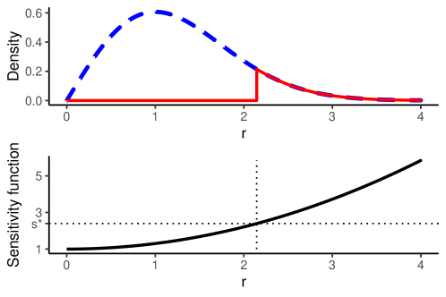
Figure 1. Density of the marginal optimal subsampling design $\xi_{R}^{*}$ on the radius (red solid) and of the marginal distribution on the radius (blue dashed) of a 2-dimensional standard normal distribution (upper panel), and sensitivity function (lower panel) for subsampling proportion $\alpha=0.1$

So far we have assumed that the covariates are centered and spherical. Let $\bm{Z}_{i}$ be such covariates that are invariant w.r.t. $SO(d)$. Now we consider covariates $\bm{X}_{i}=\bm{A}\bm{Z}_{i}+\bm{\mu}$ which are location-scale transformations of $\bm{Z}_{i}$ with non-singular transformation matrix $\bm{A}$. The covariates $\bm{X}_{i}$ have elliptical distribution with mean $\bm{\mu}$ and non-singular covariance matrix $\bm{\Sigma}_{\bm{X}}=\bm{A}\bm{A}^{\top}$. Because of equivariance of the $D$-criterion w.r.t. to such transformations, we find $D$-optimal subsampling designs in this case by transforming the observations back to the former situation by subtracting the mean $\bm{\mu}$ and multiplying with $\bm{A}^{-1}$. We show that this indeed constitutes a $D$-optimal subsampling design in the following lemma and derive the respective density in the subsequent theorem.

Lemma 3.9.

In multiple linear regression with $d\geq 2$ covariates, let the distribution of covariates $\bm{Z}_{i}\in\mathbb{R}^{d}$ be invariant w.r.t. $SO(d)$ and let $\zeta^{*}\in\Xi^{f_{\bm{Z}}}$ be the corresponding $D$-optimal subsampling design. Let $\bm{A}$ be a non-singular $d\times d$ matrix and $\bm{\mu}$ a constant in $\mathbb{R}^{d}$. Then the $D$-optimal subsampling design $\xi^{*}\in\Xi^{f_{\bm{X}}}$ for the covariates $\bm{X}_{i}=\bm{A}\bm{Z}_{i}+\bm{\mu}$ is given by $\xi^{*}(B)=\zeta^{*}(\bm{A}^{-1}(B-\bm{\mu}))$ for any measurable set $B\subset\mathbb{R}^{d}$.

Note that $\xi^{*}$ is the measure theoretic image of $\zeta^{*}$ under the transformation ${\bf z}\mapsto{\bf x}=\bm{A}{\bf z}+\bm{\mu}$.

Theorem 3.10.

In multiple linear regression with $d\geq 2$ covariates, let the distribution of the covariates $\bm{Z}_{i}\in\mathbb{R}^{d}$ be invariant w.r.t. $SO(d)$. Let $\bm{A}$ be a non-singular $d\times d$ matrix and $\bm{\mu}$ a constant in $\mathbb{R}^{d}$. Then the density of the $D$-optimal subsampling design $\xi^{*}$ for covariates $\bm{X}_{i}=\bm{A}\bm{Z}_{i}+\bm{\mu}$ is

$$f_{\xi^{*}}({\bf x})=f_{\bm{X}}({\bf x})\mathds{1}_{[q_{1-\alpha},\infty)}\left(({\bf x}-\bm{\mu})^{\top}\bm{\Sigma}^{-1}({\bf x}-\bm{\mu})\right),$$

where $\bm{\Sigma}=\bm{A}\bm{A}^{\top}$ and $q_{1-\alpha}$ is the $(1-\alpha)$-quantile of $\|\bm{Z}_{i}\|_{2}^{2}$.

To implement the continuous $D$-optimal subsampling design $\xi^{*}$ from Theorem 3.1 we suggest Algorithm 1, a simple acceptance-rejection method, where all data points that lie in the support of $\xi^{*}$ are accepted into the subdata and all others are rejected.

Data: Covariates ${\bf x}_{i},i=1,\dots,n$, mean $\bm{\mu}_{\bm{X}}$, covariance matrix $\Sigma_{\bm{X}}$.

Step 1: Calculate $c_{i}=({\bf x}_{i}-\bm{\mu}_{\bm{X}})^{\top}\bm{\Sigma}_{\bm{X}}^{-1}({\bf x}_{i}-\bm{\mu}_{\bm{X}})$;

Step 2: Select ${\bf x}_{i}$ when $c_{i}\geq q_{1-\alpha}$;

Algorithm 1 Subsample selection according to $D$-optimal subsampling design $\xi^{*}$

The resulting subsample is denoted by $({\bf x}^{\prime}_{1},\dots,{\bf x}^{\prime}_{k_{n}})$ as realization of $(\bm{X}^{\prime}_{1},\dots,\bm{X}^{\prime}_{K_{n}})$, where the $\bm{X}^{\prime}_{i}$ are i.i.d. random variables. For Algorithm 1, the subsample size $K_{n}$ is random as it depends on the $\bm{X}_{i}$, but $K_{n}$ is independent of the $\bm{X}^{\prime}_{i}$. In view of limit theorems on stopped random walks (see e. g. Gut, 2009, Theorem 1.1.) one can reasonably presume that the least squares estimator $\hat{\bm{\beta}}$ based on $(\bm{X}^{\prime}_{1},\dots,\bm{X}^{\prime}_{K_{n}})$ asymptotically follows a normal distribution with covariance matrix $\sigma_{\varepsilon}^{2}{\bf M}(\xi^{*})^{-1}$.

Example 3.11 (multivariate normal distribution).

Here we extend our findings from Example 3.8 to the case of a general multivariate normal distribution of the covariates with mean $\bm{\mu}_{\bm{X}}$ and covariance matrix $\bm{\Sigma}_{\bm{X}}$, i. e. $\bm{X}_{i}=\bm{A}\bm{Z}_{i}+\bm{\mu}_{\bm{X}}$, where $\bm{A}$ is a root of $\bm{\Sigma}_{\bm{X}}$, i. e.  $\bm{\Sigma}_{\bm{X}}=\bm{A}\bm{A}^{\top}$, and $\bm{Z}_{i}$ follows a multivariate standard normal distribution. By Theorem 3.10 we know that the $D$-optimal subsampling design is equal to the distribution of the $\bm{X}_{i}$ outside of an ellipsoid given by $({\bf x}-\bm{\mu}_{\bm{X}})^{\top}\bm{\Sigma}_{\bm{X}}^{-1}({\bf x}-\bm{\mu}_{\bm{X}})<q_{1-\alpha}$, where $q_{1-\alpha}=\chi^{2}_{d,1-\alpha}$ is equal to the $(1-\alpha)$-quantile of the $\chi^{2}$-distribution with $d$ degrees of freedom.

To guarantee the subsampling proportion $\alpha$ as well as to avoid reliance on the $(1-\alpha)$-quantile of $\|\bm{Z}_{i}\|_{2}^{2}$ in Algorithm 1 we suggest Algorithm 2. Here, the subsample size $k_{n}$ is deterministic and this algorithm only depends on the first two moments of the distribution and the distribution to be elliptical.

Let $k_{n}=[\alpha/n]$ be the integer part of $\alpha/n$;

Data: Covariates ${\bf x}_{i},i=1,\dots,n$, mean $\bm{\mu}_{\bm{X}}$, covariance matrix $\Sigma_{\bm{X}}$.

Step 1: Calculate $c_{i}=({\bf x}_{i}-\bm{\mu}_{\bm{X}})^{\top}\bm{\Sigma}_{\bm{X}}^{-1}({\bf x}_{i}-\bm{\mu}_{\bm{X}})$;

Step 2: Select ${\bf x}_{1:n},\dots,{\bf x}_{k_{n}:n}$ corresponding to the $k_{n}$ largest $c_{i}$;

Algorithm 2 Subsample selection according to design $({\bf x}_{1:n},\dots,{\bf x}_{k_{n}:n})$

The notation ${\bf x}_{i:n}$ is chosen to indicate a generalized (reverse) order statistics based on the standardized distance $c_{i}$ such that $({\bf x}_{1:n},...,{\bf x}_{n:n})$ is a permutation of $({\bf x}_{1},...,{\bf x}_{n})$ and $({\bf x}_{i:n}-\bm{\mu}_{\bm{X}})^{\top}\bm{\Sigma}_{\bm{X}}^{-1}({\bf x}_{i:n}-\bm{\mu}_{\bm{X}})\geq({\bf x}_{i+1:n}-\bm{\mu}_{\bm{X}})^{\top}\bm{\Sigma}_{\bm{X}}^{-1}({\bf x}_{i+1:n}-\bm{\mu}_{\bm{X}})$. Because the distribution of the covariates is continuous, these inequalities are strict almost surely. The selection in Step 2 of Algorithm 2 can e. g. be done using partial quicksort (see Martínez, 2004).

Remark 3.12.

For multiple linear regression the selection criterion $c_{i}=({\bf x}_{i}-\bm{\mu}_{\bm{X}})^{\top}\bm{\Sigma}_{\bm{X}}^{-1}({\bf x}_{i}-\bm{\mu}_{\bm{X}})$ for a $D$-optimal subsample is equivalent to the theoretical leverage scores $h_{i}={\bf f}({\bf x}_{i})^{\top}{\bf M}_{\bm{X}}^{-1}{\bf f}({\bf x}_{i})$, where ${\bf M}_{\bm{X}}=\operatorname{E}({\bf f}(\bm{X}_{i}){\bf f}(\bm{X}_{i})^{\top})$, as $h_{i}=c_{i}+c_{0}$, where $c_{0}=\bm{\mu}_{\bm{X}}^{\top}\bm{\Sigma}_{\bm{X}}^{-1}\bm{\mu}_{\bm{X}}\geq 0$ is a constant. Subsampling via algorithmic leveraging as described in e. g. Ma et al. (2014) uses a sampling distribution proportional to the leverage scores $h_{i}$, rather than selecting a subsample deterministically as we do here.

4. Fixed Sample Size

Unlike in the previous section, where we selected a certain percentage of the full data, we now want to select a fixed, sufficiently large, number of $k$ instances out of the total $n$ data points. This implies that we want to select a decreasing percentage $\alpha_{n}=k/n$ of the full data when $n$ increases. The subsampling design $\xi_{n}$ with total measure $\alpha_{n}$ has non-standardized (per subsample) information matrix ${\bf M}_{n}(\xi_{n})=n\int{\bf f}({\bf x}){\bf f}({\bf x})^{\top}\xi_{n}(\mathop{}\!\mathrm{d}{\bf x})$, such that $n\int\xi_{n}(\mathop{}\!\mathrm{d}{\bf x})=k$. Here we use the non-standardized information matrix to to allow for comparison of the performance for varying $n$.

If $k$ is large, the asymptotic properties in the previous section may give rise to consider the inverse information matrix ${\bf M}_{n}(\xi_{n})^{-1}$ as an approximation to the covariance matrix of $\hat{\bm{\beta}}$ based on $k$ out of $n$ observations. Hence, it seems to be reasonable to make use of the optimal continuous subsampling design $\xi_{n}^{*}$ for subsampling a proportion $\alpha_{n}=k/n$ according to Theorem 3.10. Here we adapt Algorithm 2 to select the fixed number $k_{n}=k$ data points ${\bf x}_{i}$ that correspond to the $k$ largest $c_{i}$. This design will be denoted by $({\bf x}_{1:n},...,{\bf x}_{k:n})$ with non-standardized information matrix ${\bf M}(({\bf x}_{1:n},...,{\bf x}_{k:n}))=\sum_{i=1}^{k}{\bf f}({\bf x}_{i:n}){\bf f}({\bf x}_{i:n})^{\top}$.

The computational complexity for the selection of ${\bf x}_{1:n},...,{\bf x}_{k:n}$ is $\mathcal{O}(nd^{2})$. Note that finding the inverse root of the covariance matrix is negligible, as computation of the inverse only depends on the number of covariates $d$ and we work under the assumption that $d\ll n$. Computing the least squares estimator based on $k$ observations uses computational complexity $\mathcal{O}(kd^{2})$. When $n\gg d$ it is reasonable to assume that $k\leq n/d$. Then the computational complexity for the entire procedure is $\mathcal{O}(nd^{2})$, the same magnitude as computing the least squares estimator $\hat{\bm{\beta}}$ on the full data, making it only viable in a scenario where the focus is on the expense of observing the response variable $Y_{i}$.

For scenarios where computational complexity is the main issue, we propose a second simplified method. Here we merely standardize each covariate $X_{ij}$ by its standard deviation $\sigma_{j}$. We use the matrix $\bm{\tilde{\Sigma}}_{\bm{X}}$, containing only the diagonal entries of $\bm{\Sigma}_{\bm{X}}$, for transformation of the data. To implement this we adapt Algorithm 2 by replacing the $c_{i}$ with $\tilde{c}_{i}=({\bf x}_{i}-\bm{\mu}_{\bm{X}})^{\top}\bm{\tilde{\Sigma}}_{\bm{X}}^{-1}({\bf x}_{i}-\bm{\mu}_{\bm{X}})$ and select a fixed number $k$ of points. This design will be denoted by $(\tilde{{\bf x}}_{1:n},\dots,\tilde{{\bf x}}_{k:n})$. Here, the entire procedure has computational complexity $\mathcal{O}(nd)$, as the matrix multiplication $\bm{\tilde{\Sigma}}_{\bm{X}}^{-1}({\bf x}_{i}-\bm{\mu}_{\bm{X}})$ only requires computational complexity $\mathcal{O}(nd)$, because $\bm{\tilde{\Sigma}}_{\bm{X}}^{-1}$ is a diagonal matrix. The simplified method has one more advantage. It is easier to implement in practice when there is no prior knowledge of the covariance matrix of the covariates as estimating only the variances of the covariates on a small uniform random subsample (prior to the actual subsampling procedure) is much easier than estimating the entire covariance matrix. We will see in the simulation study in Section 5 that this second method is indeed viable.

For now, however, we first want to study the performance of the initial method, where the full covariance matrix of the covariates is used for the transformation of the data. As a measure of quality of the method with a fixed sample size $k$ we use the covariance matrix $\operatorname{Cov}[\hat{\bm{\beta}};({\bf x}_{1:n},...,{\bf x}_{k:n})]$ of the least squares estimator $\hat{\bm{\beta}}$ given a subsample according to $({\bf x}_{1:n},...,{\bf x}_{k:n})$. For large $k$ the subsample size $k$ is expected to be close to the random subsample size generated by Algorithm 1 according to $\xi_{n}^{*}$, and the covariance matrix may be approximated by the inverse of the information matrix of the corresponding optimal continuous design $\xi_{n}^{*}$,

$$\operatorname{Cov}[\hat{\bm{\beta}};({\bf x}_{1:n},...,{\bf x}_{k:n})]\approx\sigma_{\varepsilon}^{2}{\bf M}_{n}(\xi_{n}^{*})^{-1}.$$ (3)

In the literature, the main interest is often only in the slope parameter $\bm{\beta}_{\mathrm{slope}}=(\beta_{1},\dots,\beta_{d})$ and the covariance matrix of the vector $\hat{\bm{\beta}}_{\mathrm{slope}}=(\hat{\beta}_{1},\dots,\hat{\beta}_{d})^{\top}$ of slope parameter estimators. Therefore, we will adopt this approach here. Note that the $D$-optimal subsampling design for $\bm{\beta}_{\mathrm{slope}}$ is the same as for the full parameter vector $\bm{\beta}$ because $\det({\bf M}^{-1})$ and the determinant of the lower right $d\times d$ submatrix of ${\bf M}^{-1}$ differ only by the constant factor $1/k$. Then, under the $D$-optimal subsampling design $\xi_{n}^{*}$ from Theorem 3.10, we find for $\bm{X}_{i}$ with mean $\bm{\mu}_{\bm{X}}$ and covariance matrix $\bm{\Sigma}_{\bm{X}}$

$$\operatorname{Cov}[\hat{\bm{\beta}}_{\mathrm{slope}};({\bf x}_{1:n},...,{\bf x}_{k:n})]\approx\sigma_{\varepsilon}^{2}(nm_{n})^{-1}\bm{\Sigma}_{\bm{X}}^{-1}\,,$$ (4)

where $m_{n}$ is the design specific term in the information matrix ${\bf M}_{n}(\zeta_{n}^{*})=n\operatorname{diag}(k/n,m_{n},\dots,m_{n})$ with $\xi_{n}^{*}(B)=\zeta_{n}^{*}(\bm{A}^{-1}(B-\bm{\mu}_{\bm{X}}))$.

Example 4.1 (multivariate standard normal distribution).

We consider the design $({\bf x}_{1:n},...,{\bf x}_{k:n})$. In the case of normally distributed covariates $\bm{X}_{i}\sim\mathcal{N}_{d}(\bm{0},\bm{\mathbb{I}}_{d})$, we find the following approximation of the covariance matrix $\operatorname{Cov}[\hat{\bm{\beta}}_{\mathrm{slope}};\xi_{k,n}^{*}]$ from equations (2) and (4)

$$\operatorname{Cov}[\hat{\bm{\beta}}_{\mathrm{slope}};({\bf x}_{1:n},...,{\bf x}_{k:n})]\approx\sigma_{\varepsilon}^{2}\left(k+\frac{2n\chi_{d,1-(k/n)}^{2}}{d}f_{\chi_{d}^{2}}(\chi_{d,1-(k/n)}^{2})\right)^{-1}\bm{\mathbb{I}}_{d}.$$ (5)

With this we can approximate the trace of the covariance matrix of $\hat{\bm{\beta}}_{\mathrm{slope}}$, which is equal to the mean squared error $\operatorname{MSE}(\hat{\bm{\beta}}_{\mathrm{slope}})=\operatorname{E}[\|\hat{\bm{\beta}}_{\mathrm{slope}}-\bm{\beta}_{\mathrm{slope}}\|_{2}^{2}]$, since the least squares estimator is unbiased. In order to compare the behavior between different dimensions $d$ we find $\operatorname{MSE}(\hat{\bm{\beta}}_{\mathrm{slope}})$ divided by $d$ is equal to any of the diagonal entries of the covariance matrix, e.g. the variance $\operatorname{Var}[\hat{\beta}_{1};({\bf x}_{1:n},...,{\bf x}_{k:n})]$ of the slope parameter estimator of the first covariate. In Figure 2 the lines depict the approximation from equation (5) of $\operatorname{MSE}(\hat{\bm{\beta}}_{\mathrm{slope}})/d$, indicated on the left vertical axis of Figure 2, for standard normal covariates in dependence of the size of the full data $n$ given a fixed size $k=1000$ of the subsample. The symbols depict the respective simulated values. The simulation procedure is given in section 5, with the only difference that the number of simulation runs $S$ for each combination of number of covariates $d$ and full sample size $n$ here is only $S=1000$, since the computations for $n=10^{7}$ take infeasibly long. We see that $\operatorname{MSE}(\hat{\bm{\beta}}_{\mathrm{slope}})/d$ tends to zero as $n\to\infty$, but substantially slower for higher dimensions $d$ as more parameters need to be estimated. Moreover, the approximation in equations (4) and (5) turn out to be useful because they are very close to the values obtained by simulation, at least, for small to moderate dimensions $d$.

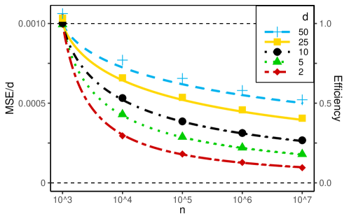
Figure 2. Approximated (lines) and simulated (symbols) MSE$/d$ of the slope parameter estimator and approximated efficiencies of uniform random subsampling (lines) in the case of standard normal covariates in dependence of the size of the full data $n$ given a fixed mean subsample size $k=1000$ and $\sigma_{\varepsilon}^{2}=1$ for various numbers of covariates $d=2,5,10,25$ and $50$

To demonstrate the advantage of the design $({\bf x}_{1:n},...,{\bf x}_{k:n})$, we consider uniform random subsampling as a natural choice to compare with. The uniform random subsampling design $\xi_{n}^{u}$ has density $f_{\xi_{n}^{u}}({\bf x})=k/nf_{\bm{X}}({\bf x})$. As a measure of quality, we study the $D$-efficiency of $\xi_{n}^{u}$ w.r.t. the $D$-optimal subsampling design $({\bf x}_{1:n},...,{\bf x}_{k:n})$. For estimating the slopes, the $D$-efficiency of a subsampling design $\xi_{n}$ with subsampling proportion $\alpha_{n}=k/n$ is defined as

$$\operatorname{eff}_{D_{\mathrm{slope}}}(\xi_{n})=\left(\frac{\det(\operatorname{Cov}[\hat{\bm{\beta}}_{\mathrm{slope}};({\bf x}_{1:n},...,{\bf x}_{k:n})])}{\det(\operatorname{Cov}[\hat{\bm{\beta}}_{\mathrm{slope}};\xi_{n}])}\right)^{1/d}$$

and can be approximated by replacing the covariances by the inverse information matrices for the slopes. For this definition the homogeneous version $(\det(\operatorname{Cov}[\hat{\bm{\beta}}_{\mathrm{slope}};\xi_{n}]))^{1/d}$ of the $D$-criterion is used, satisfying the homogeneity condition $(\det(\lambda\operatorname{Cov}[\hat{\bm{\beta}}_{\mathrm{slope}};\xi_{n}]))^{1/d}=\lambda(\det(\operatorname{Cov}[\hat{\bm{\beta}}_{\mathrm{slope}};\xi_{n}]))^{1/d}$ for all $\lambda>0$ (see Pukelsheim, 1993, Chapter 6.2).

As mentioned in Reuter and Schwabe (2023), the $D$-efficiency $\operatorname{eff}_{D_{\mathrm{slope}}}(\xi_{n}^{u})$ of uniform random subsampling can be nicely interpreted: the sample size required to obtain the same precision (in terms of the $D_{\mathrm{slope}}$-criterion), as when the $D_{\mathrm{slope}}$-optimal subsampling design $\xi_{n}^{*}$ with subsample size $k$ is used, is equal to the inverse of the efficiency $\operatorname{eff}_{D_{\mathrm{slope}}}(\xi_{n}^{u})$ times $k$. For example, if the efficiency $\operatorname{eff}_{D_{\mathrm{slope}}}(\xi_{n}^{u})$ is equal to $0.5$, then twice as many observations would be needed under uniform random sampling than for a $D_{\mathrm{slope}}$-optimal subsampling design. The information matrix for uniform random subsampling is given by ${\bf M}_{n}(\xi_{n}^{u})=k\int{\bf f}({\bf x}){\bf f}({\bf x})^{\top}f_{\bm{X}}({\bf x})\mathop{}\!\mathrm{d}{\bf x}=k\operatorname{diag}(1,\Sigma_{\bm{X}})$.

Corollary 4.2.

The $D_{\mathrm{slope}}$-efficiency of the design $({\bf x}_{1:n},...,{\bf x}_{k:n})$ can be approximated by $\operatorname{eff}_{D_{\mathrm{slope}}}(\xi_{n}^{u})\approx k/(nm_{n})$, where $m_{n}$ are the diagonal entries of ${\bf M}_{n}(\zeta_{n}^{*})=n\operatorname{diag}(k/n,m_{n},\dots,m_{n})$.

Example 4.3 (normal distribution).

Consider $\bm{X}_{i}\sim\mathcal{N}_{d}(\bm{\mu}_{\bm{X}},\bm{\Sigma}_{\bm{X}})$. By Corollary 4.2 we have $\operatorname{eff}_{D_{\mathrm{slope}}}(\xi_{n}^{u})\approx k/(nm_{n})$, where

$$m_{n}=\frac{k}{n}+\frac{2\chi^{2}_{d,1-\alpha}}{d}f_{\chi^{2}_{d}}(\chi^{2}_{d,1-\alpha}),$$

from equation (2). The approximated efficiency $\operatorname{eff}_{D_{\mathrm{slope}}}(\xi_{n}^{u})$ is thus equal to the approximated $\operatorname{MSE}(\hat{\bm{\beta}}_{\mathrm{slope}})/d$ given the design $({\bf x}_{1:n},...,{\bf x}_{k:n})$ as depicted in Figure 2, multiplied by $k/\sigma_{\varepsilon}^{2}$. The efficiency ranges between zero and one and is indicated by the vertical axis on the right of Figure 2.

5. Simulation Study

We divide our simulation study into two parts. First, we study the performance of the optimal subsampling designs $({\bf x}_{1:n},\dots,{\bf x}_{k:n})$ derived from Theorem 3.10 in the case of multivariate normally distributed and multivariate $t$-distributed covariates with three degrees of freedom, respectively, both with and without correlation between the covariates. For the $t$-distribution, we choose three degrees of freedom to maximize dispersion, while maintaining existence of the variance. Second, we use the simplified design $(\tilde{{\bf x}}_{1:n},\dots,\tilde{{\bf x}}_{k:n})$ discussed in Section 4 that only takes the variance of the covariates into account while ignoring the correlation. The latter has lower computational complexity, $\mathcal{O}(nd)$. For better comparability, the simulation is structured similar to those in the work by Wang et al. (2019). The data is generated from the linear model $Y_{i}=\beta_{0}+\bm{X}_{i}^{\top}\bm{\beta}_{\mathrm{slope}}+\varepsilon_{i},\;i=1,\dots,n,$ with $d=50$. The parameter vector $\bm{\beta}$ was generated from a multivariate normal distribution in each iteration. Note, however, that the value of $\bm{\beta}$ does not have any influence on the results. For the errors we choose independent $\varepsilon_{i}\sim\mathcal{N}(0,1)$. The subdata is of fixed size $k=1000$, whereas the size of the full data takes the values $n=5000,10000,100000$, and one million. For each value of $n$, we apply our subsampling methods and calculate the least squares estimator $\hat{\bm{\beta}}$ for each method. We repeat this $S=10000$ times. We select subdata based on our approach (D-OPT) and the IBOSS method (IBOSS) by Wang et al. (2019). Further we select subdata by uniform sampling (UNIF) and give a comparison to estimates based on the full data (FULL) to give context to our approach and the IBOSS method. In each iteration s, we form the subsample in the $k\times d$ matrix $\bm{X}_{(s)}$ (based on the respective method) and calculate its inverse information matrix $\mathcal{C}_{(s)}=((\bm{1}_{k},\bm{X}_{(s)})^{\top}(\bm{1}_{k},\bm{X}_{(s)}))^{-1}$, where $\bm{1}_{k}$ is a $k$-dimensional vector with all entries equal to one. We then take the average of these $(d+1)\times(d+1)$ covariance matrices $\mathcal{C}=1/S\sum_{s=1}^{S}\mathcal{C}_{(s)}$ and partition this matrix the following way.

$$\mathcal{C}=\begin{pmatrix}c_{0}&\bm{c}_{1}^{\top}\\ \bm{c}_{1}&\mathcal{C}_{1},\end{pmatrix}$$

where $c_{0}\geq 1/k$ with equality if $\bm{c}_{1}=\bm{0}$. The submatrix $\mathcal{C}_{1}$ is of dimension $d\times d$. Note that $\mathcal{C}$ and $\mathcal{C}_{1}$ are the simulated covariance matrices of $\bm{\beta}$ and $\bm{\beta}_{\mathrm{slope}}$, respectively. The mean of the covariance matrices is taken instead of the mean of the information matrices, which has been the target quantity for asymptotic behavior. Note that the inverse of the mean information matrix is a lower bound for the mean covariance matrix by Jensen’s inequality. Then, we calculate the determinant of $\mathcal{C}_{1}$ and scale it to homogeneity, i. e. $\det(\mathcal{C}_{1})^{(1/d)}$. Alternatively to using $\det(\mathcal{C}_{1})^{(1/d)}$ to compare the different methods, we have also used the MSE of $\hat{\bm{\beta}}_{\mathrm{\mathrm{slope}}}$, i. e. $\operatorname{MSE}_{\bm{\hat{\beta}}_{\mathrm{slope}}}=S^{-1}\sum_{s=1}^{S}\|\bm{\hat{\beta}}_{\mathrm{slope}}^{(s)}-\bm{\beta}_{\mathrm{slope}}\|_{2}^{2}$, where $\bm{\hat{\beta}}_{\mathrm{slope}}^{(s)}$ is the estimator of the $s$-th iteration. Results were very similar in all cases and, importantly, the comparison between them does not change. In particular note that the trace of $\mathcal{C}_{1}$ is equal to $\operatorname{MSE}_{\hat{\bm{\beta}}_{\mathrm{slope}}}$.

Consider the special case of homoscedastic covariates. Then all diagonal elements of the theoretical counterpart of $\operatorname{Cov}(\hat{\bm{\beta}}_{\mathrm{slope}})$ are equal and all off-diagonal entries are equal to zero. Thus in theory we have the MSE divided by $d$ is equal to the term of interest $\det(\operatorname{Cov}(\hat{\bm{\beta}}_{\mathrm{slope}}))^{1/d}$ in our simulations. In this situation, the $D$-optimal subsampling design is equal to the $A$-optimal subsampling design for the slope parameters, which minimizes $\operatorname{trace}(\operatorname{Cov}(\hat{\bm{\beta}}_{\mathrm{slope}}))$ and thus the MSE. As $A$- and $D$-optimal subsampling designs are not equal in other cases we recommend using an $A$-optimal subsampling design as a benchmark for other methods when the MSE is used as the measure of comparison, but we will not follow this line further here. All simulations are performed using R Statistical Software (R Core Team, 2023, v4.2.2).

5.1. Optimal Subsampling Design $({\bf x}_{1:n},\dots,{\bf x}_{k:n})$

Here we use the subsampling design $({\bf x}_{1:n},\dots,{\bf x}_{k:n})$ from Algorithm 2 with fixed $k$. Let $\bm{\Sigma}_{\bm{X}}=\bm{\mathbb{I}}_{50}$ or $\bm{\Sigma}_{0.5}$, where $\bm{\Sigma}_{0.5}=(\bm{\mathbb{I}}_{50}+\bm{1}_{50}\bm{1}_{50}^{\top})/2$ represents compound symmetry with correlation $\rho=0.5$. Figure 3 shows the results for normally distributed covariates $\bm{X}_{i}$ with $\bm{\mathbb{I}}_{50}$ and $\bm{\Sigma}_{0.5}$ as the covariance matrix respectively. Figure 4 shows the results for the $t$-distribution with three degrees of freedom where $\bm{\mathbb{I}}_{50}$ and $\bm{\Sigma}_{0.5}$ are the respective scale matrices, so again we have compound symmetry with correlation $\rho=0.5$ in the latter case. Here, we omit the uniformly selected subsample for better visibility because uniform subsampling performs substantially worse. For uniform random subsampling, the determinant is close to constant at around $4.6\times 10^{-4}$ for all four values of $n$ in the case of no correlation and similarly around $8.5\times 10^{-4}$ in the case with correlation.

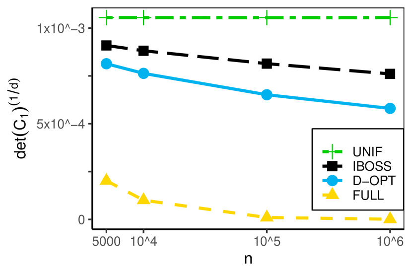
(a) $\bm{X}_{i}\sim\mathcal{N}\left(\bm{0},\bm{\mathbb{I}}_{50}\right)$.

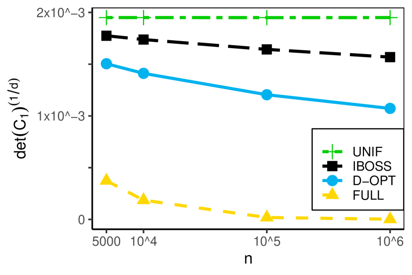
(b) $\bm{X}_{i}\sim\mathcal{N}\left(\bm{0},\bm{\Sigma}_{0.5}\right)$.

Figure 3. Standardized determinant of the inverse information matrix for normally distributed covariates given different covariance matrices.

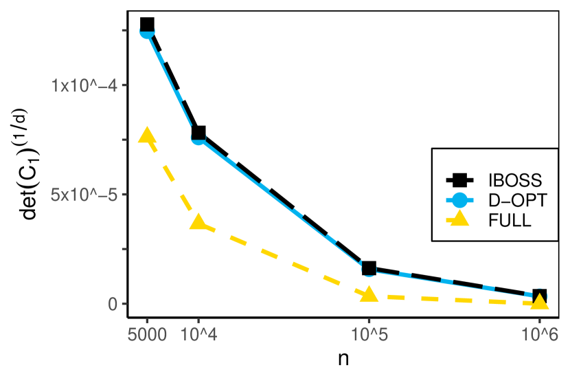
(a) $\bm{X}_{i}\sim t_{3}\left(\bm{0},\bm{\mathbb{I}}_{50}\right)$

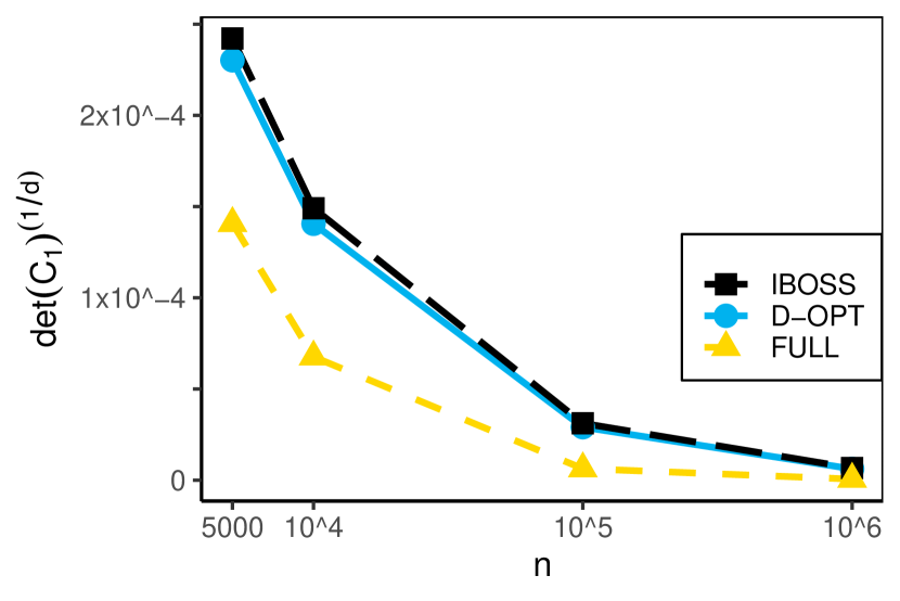
(b) $\bm{X}_{i}\sim t_{3}\left(\bm{0},\bm{\Sigma}_{0.5}\right)$.

Figure 4. Standardized determinant of the inverse information matrix for $t$-distributed covariates with three degrees of freedom given different scale matrices

As expected, regardless of the distribution of the covariates, for uniform random subsampling the full sample size $n$ has no impact on $\det(\mathcal{C}_{1})^{(1/d)}$, which is equal to $n/k$ times that value of the full data.

With the prior knowledge of the distribution of the covariates, our method is able to outperform the IBOSS method. As is to be expected, our approach can increase its advantage over the IBOSS method when there is correlation between the covariates. The advantage is however minor for the heavy-tailed $t$-distribution, where both methods perform much closer to the full data. In particular, for large $n$ both perform basically as good as the full data. For reference, in the case of positive correlations the relative efficiency of the IBOSS method with respect to the D-OPT method, i.e. the ratio of the corresponding values of D-OPT divided by IBOSS, ranges from approximately 0.951 to 0.928 for the different values in full sample size $n$.

5.2. Simplified Method $(\tilde{{\bf x}}_{1:n},\dots,\tilde{{\bf x}}_{k:n})$

Finally, we want to study the simplified design $(\tilde{{\bf x}}_{1:n},\dots,\tilde{{\bf x}}_{k:n})$ of the D-OPT method that only scales by standard deviations and can be performed in $\mathcal{O}(nd)$. In this method, we ignore the correlations between the covariates. We use the diagonal matrix $\bm{\tilde{\Sigma}}=\operatorname{diag}(\sigma_{1}^{2},\dots,\sigma_{d}^{2})$ containing only the diagonal entries of $\bm{\Sigma}_{\bm{X}}$ for transformation of the data, such that the entire procedure has computational complexity $\mathcal{O}(nd)$. We examine this method in the case of normally distributed covariates and refer to the simplified D-OPT method as “D-OPT-s” in the figures.

Note that in the case of no correlation between the covariates the simplified method is equal to the D-OPT method of the previous section. Thus results for this scenario can be inherited from Figure 3(A). Further, we consider compound symmetry with $\rho=0.05$ and $\rho=0.5$. The $50\times 50$ covariance matrices of the $\bm{X}_{i}$ are $\bm{\Sigma}_{\bm{X}}=\bm{\Sigma}_{0.05}$ or $\bm{\Sigma}_{0.5}$, with $\sigma_{0.05,ii}=1$ and $\sigma_{0.05,ij}=0.05$ for $i\neq j$ and $\bm{\Sigma}_{0.5}$ as before. Figure 5 shows the results for normally distributed covariates $\bm{X}_{i}$ with $\bm{\Sigma}_{0.05}$ and $\bm{\Sigma}_{0.5}$ as the covariance matrix, respectively. While the advantage of the $D$-optimal subsampling design over the IBOSS method is reduced, there are still scenarios where it can outperform the IBOSS method such as the one of covariance matrix $\bm{\Sigma}_{0.05}$ with small correlations. However, if correlations are particularly large as in the case of covariance matrix $\bm{\Sigma}_{0.5}$, the simplified method D-OPT-s seems to perform much worse and only slightly outperforms uniform subsampling.

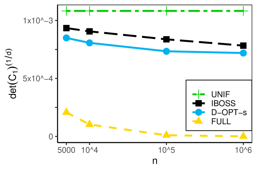
(a) $\bm{X}_{i}\sim\mathcal{N}\left(\bm{0},\bm{\Sigma}_{0.05}\right)$.

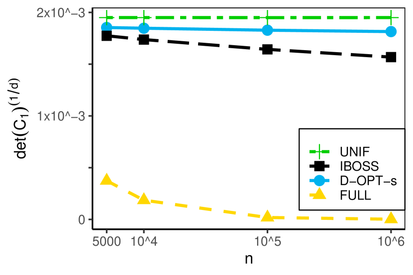
(b) $\bm{X}_{i}\sim\mathcal{N}\left(\bm{0},\bm{\Sigma}_{0.5}\right)$.

Figure 5. Standardized determinant of the inverse information matrix for normally distributed covariates given different covariance matrices for the simplified D-OPT-s method

6. Concluding Remarks

We have constructed optimal subsampling designs $\xi^{*}$ for multiple linear regression, first for centered spherical distributions, then for distributions that can be generated from such a distribution via location-scale transformation. We have given two methods of implementation and discussed that the computational complexity of the $D$-optimal method, that selects the $k$ data points with the largest Mahalanobis distance from the mean of the data, is $\mathcal{O}(nd^{2})$, whereas the simplified version can be performed in $\mathcal{O}(nd)$. We have compared these implementations to the IBOSS method of Wang et al. (2019) in simulation studies with the expected result that the full method outperforms IBOSS as well as the simplified method outperforms the IBOSS method in certain settings with small correlations between the covariates. Besides applications where the covariance matrix of the covariates is known, our method can be used as a benchmark for other methods that do not require prior knowledge of the distribution of the covariates. Note, that the proposed subsampling designs depend both on the distribution of the covariates and the model. If either is incorrect, the subsampling designs will no longer be optimal. Recent work on subsampling for model discrimination is done by Yu and Wang (2022).

Appendix A Technical Details

Lemma A.1.

The essential part of the directional derivative

$$F_{\Psi}(\xi,\xi_{{\bf x}})=\lim_{\epsilon\to 0^{+}}\frac{1}{\epsilon}\left(-\log(\det({\bf M}((1-\epsilon)\xi+\epsilon\xi_{{\bf x}})))+\log(\det({\bf M}(\xi)))\right)$$

at a design $\xi$ in the direction of a one-point measure $\xi_{{\bf x}}$ with total measure $\alpha$ is the sensitivity function $\psi({\bf x},\xi)=(d+1)-F_{\Psi}(\xi,\xi_{{\bf x}})=\alpha{\bf f}({\bf x})^{\top}{\bf M}(\xi)^{-1}{\bf f}({\bf x})$.

Proof of Lemma A.1.

The directional derivative $F_{\Psi}(\xi,\xi_{{\bf x}})$ can be calculated as $F_{\Psi}(\xi,\xi_{{\bf x}})=(d+1)-\operatorname{Tr}({\bf M}(\xi)^{-1}{\bf M}(\xi_{{\bf x}}))$ (see Silvey, 1980, Example 3.8) which reduces to $F_{\Psi}(\xi,\xi_{{\bf x}})=(d+1)-\alpha{\bf f}({\bf x})^{\top}{\bf M}(\xi)^{-1}{\bf f}({\bf x})$ for a one-point measure $\xi_{{\bf x}}$. Equivalently, we consider the sensitivity function $\psi({\bf x},\xi)=\alpha{\bf f}({\bf x})^{\top}{\bf M}(\xi)^{-1}{\bf f}({\bf x})$, which incorporates the essential part of the directional derivative ($\psi({\bf x},\xi)=(d+1)-F_{\Psi}(\xi,\xi_{{\bf x}})$). ∎

Remark A.2.

For the representation of a design $\xi$ in hyperspherical coordinates we make use of the transformation $T:[0,\infty)\times[0,\pi]^{d-2}\times[0,2\pi)\to\mathbb{R}^{d},T(r,\bm{\theta})={\bf x}$, where $\bm{\theta}=(\theta_{1},\dots,\theta_{d-1})^{\top}$, $x_{k}=r\cos(\theta_{k})\prod_{j=1}^{k-1}\sin(\theta_{j})$ for $k=1,\dots,d-1$, and $x_{d}=r\prod_{j=1}^{d-1}\sin(\theta_{j})$. We identify all points with radius zero with the origin and denote the inverse of the transformation $T$ by $S=T^{-1}$. Then, for a subsampling design $\xi\in\Xi^{f_{\bm{X}}}$ on $\mathbb{R}^{d}$, the induced subsampling design $\xi^{S}$ is the same subsampling design in hyperspherical coordinates, i. e. on $[0,\infty)\times\mathbb{B}$, where $\mathbb{B}=[0,\pi]^{d-2}\times[0,2\pi)$.

Proof of Theorem 3.1.

The result follows immediately from Corollary 1 (c) in Sahm and Schwabe (2001) as in Theorem 3.1. in Reuter and Schwabe (2023). ∎

Proof of Lemma 3.3.

We define $\mathbb{h}$ as a mapping from $\mathbb{R}_{>0}\times\mathbb{B}$ to itself. Let $\mathbb{h}=(h_{0},\mathbb{h}_{1}^{\top})^{\top}$, where $h_{0}(r)=r$ is the identity on the radius and $\mathbb{h}_{1}\in SO(d)$ acts on the angle $\bm{\theta}$. First note that for any $B=B_{R}\times B_{\bm{\Theta}}$ with $B_{R}\in\mathcal{B}(\mathbb{R}_{>0})$ and $B_{\bm{\Theta}}\in\mathcal{B}(\mathbb{B})$ and any $\mathbb{h}_{1}\in SO(d)$ the mapping $\mathbb{h}$ only affects the set $B_{\bm{\Theta}}$ on the angle. Since $\mu$ is a left Haar measure w.r.t $SO(d)$, it holds that $\mu(\mathbb{h}_{1}^{-1}(B_{\bm{\Theta}}))=\mu(B_{\bm{\Theta}})$ for any $\mathbb{h}_{1}\in SO(d)$ and any $B_{\bm{\Theta}}\in\mathcal{B}(\mathbb{B})$. We first prove that the composition $\xi=\xi_{R}\otimes\mu$ of a measure $\xi_{R}$ on the radius and the Haar measure $\mu$ implies invariance. For any $B=B_{R}\times B_{\bm{\Theta}}$ and any $\mathbb{h}_{1}\in SO(d)$, we have

$$\xi^{\mathbb{h}}(B) =(\xi_{R}\otimes\mu)(\mathbb{h}^{-1}(B_{R}\times B_{\bm{\Theta}}))$$

$$=\xi_{R}(B_{R})\mu(\mathbb{h}_{1}^{-1}(B_{\bm{\Theta}}))$$

$$=\xi_{R}(B_{R})\mu(B_{\bm{\Theta}})$$

$$=\xi(B).$$

Because the $\sigma$-algebra $\mathcal{B}(\mathbb{R}_{>0})\otimes\mathcal{B}(\mathbb{B})$ is generated by $\mathcal{B}(\mathbb{R}_{>0})\times\mathcal{B}(\mathbb{B})$, we conclude that $\xi$ is invariant w.r.t. $SO(d)$.

Conversely, let us assume $\xi=\xi_{R}\otimes\xi_{\bm{\Theta}|R}$ (this decomposition exists by the Radon–Nikodym Theorem) is invariant w.r.t. $SO(d)$ and there exist sets $B_{R}\in\mathcal{B}(\mathbb{R}_{>0})$ with $\xi_{R}(B_{R})>0$ and $B_{\bm{\Theta}}\in\mathcal{B}(\mathbb{B})$ such that $\xi_{\bm{\Theta}|R\in B_{R}}(B_{\bm{\Theta}})\neq\mu(B_{\bm{\Theta}})>0$. Then there exists a rotation $\mathbb{h}_{1}\in SO(d)$ such that $\xi_{\bm{\Theta}|R\in B_{R}}(B_{\bm{\Theta}})\neq\xi_{\bm{\Theta}|R\in B_{R}}(\mathbb{h}_{1}^{-1}(B_{\bm{\Theta}}))$, and subsequently we have $\xi^{\mathbb{h}}(B_{R}\times B_{\bm{\Theta}})\neq\xi(B_{R}\times B_{\bm{\Theta}})$. This contradicts the invariance assumption and we derive that invariance of $\xi$ w.r.t. $SO(d)$ implies that $\xi_{\bm{\Theta}|R}(B_{\bm{\Theta}})=\mu(B_{\bm{\Theta}})$ almost everywhere w.r.t. $\xi_{R}$. This concludes the proof. ∎

Proof of Lemma 3.4.

The $\bm{X}_{i}$ are invariant w.r.t. $SO(d)$ and thus we can write the density of the $\bm{X}_{i}$ as $f_{\bm{X}}({\bf x})=f_{R(\bm{X})}(r)f_{\mu}(\bm{\theta})$ by Lemma 3.3. We can decompose the density of $\xi$ into $f_{\xi}({\bf x})=f_{R(\xi)}(r)f_{\bm{\Theta}|R}(\bm{\theta})$. We have $f_{R(\xi)}(r)\leq f_{R(\bm{X})}(r)$ because $\xi\in\Xi^{f_{\bm{X}}}$. As a result $f_{\overline{\xi}}({\bf x})=f_{R(\xi)}(r)f_{\mu}(\bm{\theta})\leq f_{R(\bm{X})}(r)f_{\mu}(\bm{\theta})$ and thus $\overline{\xi}\in\Xi^{f_{\bm{X}}}$. ∎

Proof of Lemma 3.5.

Consider the information matrix of a subsampling design $\xi$ in hyperspherical coordinates, i. e. with the transformation $T$ and its inverse $S$. The Jacobi matrix of $T$ is denoted by $\bm{J}_{T}(r,\bm{\theta})$. Then

$${\bf M}(\xi) =\int_{\mathbb{R}^{d}}{\bf f}({\bf x}){\bf f}({\bf x})^{\top}\xi(\mathop{}\!\mathrm{d}{\bf x})$$

$$=\int_{S(\mathbb{R}^{d})}{\bf f}(T(r,\bm{\theta})){\bf f}(T(r,\bm{\theta}))^{\top}\xi^{S}(\mathop{}\!\mathrm{d}(r,\bm{\theta}))$$

$$=\int_{[0,\infty)}\int_{\mathbb{B}}{\bf f}(T(r,\bm{\theta})){\bf f}(T(r,\bm{\theta}))^{\top}|\det(\bm{J}_{T}(r,\bm{\theta}))|\xi_{\bm{\Theta}|R=r}(\mathop{}\!\mathrm{d}\bm{\theta})\xi_{R}(\mathop{}\!\mathrm{d}r).$$

Now we study the sum of information matrices of rotated subsampling designs.

$$\frac{1}{|G|}\sum_{g\in G}{\bf M}(\xi^{g}) =\frac{1}{|G|}\sum_{g\in G}\int_{[0,\infty)}\int_{\mathbb{B}}{\bf f}(T(r,\bm{\theta})){\bf f}(T(r,\bm{\theta}))^{\top}|\det(\bm{J}_{T}(r,\bm{\theta}))|\xi^{g}_{\bm{\Theta}|R=r}(\mathop{}\!\mathrm{d}\bm{\theta})\xi_{R}(\mathop{}\!\mathrm{d}r)$$

$$=\frac{1}{|G|}\sum_{g\in G}\int_{[0,\infty)}\int_{\mathbb{B}}{\bf f}(g^{-1}(T(r,\bm{\theta}))){\bf f}(g^{-1}(T(r,\bm{\theta})))^{\top}|\det(\bm{J}_{T}(r,\bm{\theta}))|\xi_{\bm{\Theta}|R=r}(\mathop{}\!\mathrm{d}\bm{\theta})\xi_{R}(\mathop{}\!\mathrm{d}r)$$

$$=\int_{[0,\infty)}\int_{\mathbb{B}}\sum_{g\in G}\frac{1}{|G|}{\bf f}(g^{-1}(T(r,\bm{\theta}))){\bf f}(g^{-1}(T(r,\bm{\theta})))^{\top}|\det(\bm{J}_{T}(r,\bm{\theta}))|\xi_{\bm{\Theta}|R=r}(\mathop{}\!\mathrm{d}\bm{\theta})\xi_{R}(\mathop{}\!\mathrm{d}r).$$

The inner sum can be regarded as the information matrix of a design putting equal weight on the vertices of a rotated $$d d$$-dimensional cross-polytope. This is equal to the information matrix of the uniform distribution on the -sphere, see Pukelsheim (1993, Chapter 15.18.) or Gaffke and Heiligers (1996, Lemma 4.9.). Then

$$\frac{1}{|G|}\sum_{g\in G}{\bf M}(\xi^{g}) =\int_{[0,\infty)}\int_{\mathbb{B}}\int_{\mathbb{B}}{\bf f}(T(r,\bm{\gamma})){\bf f}(T(r,\bm{\gamma}))^{\top}|\det(\bm{J}_{T}(r,\bm{\gamma}))|\mu(\mathop{}\!\mathrm{d}\bm{\gamma})\xi_{\bm{\Theta}|R=r}(\mathop{}\!\mathrm{d}\bm{\theta})\xi_{R}(\mathop{}\!\mathrm{d}r)$$

$$=\int_{[0,\infty)}\int_{\mathbb{B}}{\bf f}(T(r,\bm{\gamma})){\bf f}(T(r,\bm{\gamma}))^{\top}|\det(\bm{J}_{T}(r,\bm{\gamma}))|\mu(\mathop{}\!\mathrm{d}\bm{\gamma})\int_{\mathbb{B}}\xi_{\bm{\Theta}|R=r}(\mathop{}\!\mathrm{d}\bm{\theta})\xi_{R}(\mathop{}\!\mathrm{d}r)$$

$$=\int_{[0,\infty)}\int_{\mathbb{B}}{\bf f}(T(r,\bm{\gamma})){\bf f}(T(r,\bm{\gamma}))^{\top}|\det(\bm{J}_{T}(r,\bm{\gamma}))|\mu(\mathop{}\!\mathrm{d}\bm{\gamma})\xi_{R}(\mathop{}\!\mathrm{d}r)$$

$$={\bf M}(\xi_{R}\otimes\mu).$$

In the third equality we used $\int_{\mathbb{B}}\xi_{\bm{\Theta}|R=r}(\mathop{}\!\mathrm{d}\bm{\theta})=1$. ∎

Proof of Theorem 3.6.

By the result ${\bf M}(\overline{\xi})=\frac{1}{|G|}\sum_{g\in G}{\bf M}(\xi^{g})$ of Lemma 3.5 we have

$$\Phi({\bf M}(\overline{\xi})) \leq\frac{1}{|G|}\sum_{g\in G}\Phi({\bf M}(\xi^{g}))$$

by the convexity of $$\Phi g\in G\subset SO(d) \Phi SO(d) \Phi({\bf M}(\xi^{g}))=\Phi({\bf M}(\xi))$$. Note that . We then utilize that is invariant w.r.t. , i. e. , and obtain

$$\Phi({\bf M}(\overline{\xi})) \leq\Phi({\bf M}(\xi)).$$

∎

Proof of Theorem 3.7.

We apply Theorem 3.1. $\xi^{*}$ is defined such that it is equal to the bounding distribution on $\mathcal{X}^{*}=\{{\bf x}\in\mathcal{X}:\|{\bf x}\|^{2}_{2}\geq q_{1-\alpha}\}$ and equal to zero on $\{{\bf x}\in\mathcal{X}:\|{\bf x}\|^{2}_{2}<q_{1-\alpha}\}$. The sensitivity function from equation (1) is

$$\psi({\bf x},\xi^{*})=1+\frac{\alpha}{m}\|{\bf x}\|_{2}^{2}.$$

Then we can immediately see that $s^{*}=\inf_{x\in\mathcal{X}^{*}}\psi({\bf x},\xi^{*})=\sup_{x\notin\mathcal{X}^{*}}\psi({\bf x},\xi^{*})=\frac{\alpha}{m}q_{1-\alpha}.$ and thus conditions (i)-(iii) are satisfied, which concludes the proof. ∎

Proof of Lemma 3.9.

Note that for any $d\times d$ matrix $\bm{A}$ and any vector $\bm{\mu}\in\mathbb{R}^{d}$, there exists a bijection $\Xi^{f_{\bm{Z}}}\to\Xi^{f_{\bm{X}}}$, where every subsampling design $\zeta\in\Xi^{f_{\bm{Z}}}$ is mapped to $\xi\in\Xi^{f_{\bm{X}}}$, which is defined as $\xi(B)=\zeta(\bm{A}^{-1}(B-\bm{\mu}))$ for any measurable set $B\subset\mathbb{R}^{d}$. Let $\zeta\in\Xi^{f_{\bm{Z}}}$. Consider the information matrix of the subsampling design $\xi$,

$${\bf M}(\xi) =\int{\bf f}({\bf x}){\bf f}({\bf x})^{\top}\xi(\mathop{}\!\mathrm{d}{\bf x})$$

$$=\int{\bf f}(\bm{A}{\bf z}+\bm{\mu}){\bf f}(\bm{A}{\bf z}+\bm{\mu})^{\top}\zeta(\mathop{}\!\mathrm{d}{\bf z})$$

$$=\int\begin{pmatrix}1&\bm{0}^{\top}\\ \bm{\mu}&\bm{A}\end{pmatrix}{\bf f}({\bf z}){\bf f}({\bf z})^{\top}\begin{pmatrix}1&\bm{\mu}^{\top}\\ \bm{0}&\bm{A}^{\top}\end{pmatrix}\zeta(\mathop{}\!\mathrm{d}{\bf z})$$

$$=\begin{pmatrix}1&\bm{0}^{\top}\\ \bm{\mu}&\bm{A}\end{pmatrix}{\bf M}(\zeta)\begin{pmatrix}1&\bm{\mu}^{\top}\\ \bm{0}&\bm{A}^{\top}\end{pmatrix}.$$

The determinant of the information matrix can be calculated as follows.

$$\det\left({\bf M}(\xi)\right) =\det(\bm{A}\bm{A}^{\top})\det\left({\bf M}(\zeta)\right).$$

Thus $\xi^{*}$ minimizes $\Psi(\xi)$ in $\Xi^{f_{\bm{X}}}$, if $\zeta^{*}$ minimizes $\Psi(\zeta)$ in $\Xi^{f_{\bm{Z}}}$. ∎

Proof of Theorem 3.10.

From Lemma 3.9 we have that $\xi^{*}(B)=\zeta^{*}(\bm{A}^{-1}(B-\bm{\mu}))$ for any measurable set $B\subset\mathbb{R}^{d}$, where $\zeta^{*}$ is the optimal subsampling design for covariates $\bm{Z}_{i}$ in the setting of Theorem 3.7. We inherit the desired result by applying Theorem 3.7. ∎

Proof of equation (2).

Let $\bm{X}_{i}=(X_{i,1},\dots,X_{i,d})^{\top}\sim\mathcal{N}_{d}\left(\bm{0},\mathbb{I}_{d}\right)$ with density $f_{\bm{X}}$. From Theorem 3.7, we know that the support of $\xi^{*}$ is $\mathcal{X}^{*}=\{{\bf x}\in\mathbb{R}^{d}:\|{\bf x}\|^{2}_{2}\geq\chi^{2}_{d,1-\alpha}\}$ on which it is equal to the $d$-dimensional standard normal distribution. By definition, the information matrix of $\xi^{*}$ is ${\bf M}(\xi^{*})=\int{\bf f}({\bf x}){\bf f}({\bf x})^{\top}\xi^{*}(\mathop{}\!\mathrm{d}{\bf x})$. Any off-diagonal entries $\int x_{j}\xi^{*}(\mathop{}\!\mathrm{d}{\bf x})$ and $\int x_{j}x_{j^{\prime}}\xi^{*}(\mathop{}\!\mathrm{d}{\bf x})$, $j,j^{\prime}=1,\dots,d,j\neq j^{\prime}$ are equal to zero. The upper left element of the matrix is $\xi^{*}(\mathbb{R}^{d})=\alpha$ by the definition of a subsampling design. The other elements on the main diagonal are equal because $\xi^{*}$ is invariant w.r.t. $SO(d)$ and thus $\int x_{j}^{2}\xi^{*}(\mathop{}\!\mathrm{d}{\bf x})=\int x_{j^{\prime}}^{2}\xi^{*}(\mathop{}\!\mathrm{d}{\bf x})$ for any $j,j^{\prime}=1,\dots,d$. Note that $W=\|\bm{X}_{i}\|^{2}_{2}$ follows a $\chi^{2}$-distribution with $d$ degrees of freedom. We start to calculate $m$ by formulating it as the expected value of $W$.

$$m =\int_{\mathcal{X}^{*}}x_{1}^{2}f_{\bm{X}}({\bf x})\mathop{}\!\mathrm{d}{\bf x}$$

$$=\operatorname{E}\left[X_{i,1}^{2}\mathds{1}_{\{\|\bm{X}_{i}\|^{2}_{2}\geq\chi^{2}_{d,1-\alpha}\}}\right]$$

$$=\frac{1}{d}\operatorname{E}\left[\|\bm{X}_{i}\|^{2}_{2}\mathds{1}_{\{\|\bm{X}_{i}\|^{2}_{2}\geq\chi^{2}_{d,1-\alpha}\}}\right]$$

$$=\frac{1}{d}\operatorname{E}\left[W\mathds{1}_{\{W\geq\chi^{2}_{d,1-\alpha}\}}\right].$$

We write the expected value in its integral form and insert the density $$f_{\chi^{2}_{d}} \chi^{2} d$$ of the -distribution with degrees of freedom. Then

$$m =\frac{1}{d}\int_{\chi^{2}_{d,1-\alpha}}^{\infty}wf_{\chi^{2}_{d}}(w)\mathop{}\!\mathrm{d}w$$

$$=\frac{1}{d2^{d/2}\Gamma(d/2)}\int_{\chi^{2}_{d,1-\alpha}}^{\infty}w^{d/2}e^{-w/2}\mathop{}\!\mathrm{d}w.$$

Integration by parts yields

$$m =\frac{1}{d2^{d/2}\Gamma(d/2)}\left(2(\chi^{2}_{d,1-\alpha})^{d/2}e^{-\chi^{2}_{d,1-\alpha}/2}+d\int_{\chi^{2}_{d,1-\alpha}}^{\infty}w^{(d/2)-1}e^{-w/2}\mathop{}\!\mathrm{d}w\right)$$

$$=\frac{(\chi^{2}_{d,1-\alpha})^{d/2}e^{-\chi^{2}_{d,1-\alpha}/2}}{d2^{(d/2)-1}\Gamma(d/2)}+\int_{\chi^{2}_{d,1-\alpha}}^{\infty}\frac{w^{(d/2)-1}e^{-w/2}}{2^{d/2}\Gamma(d/2)}\mathop{}\!\mathrm{d}w.$$

The latter term simplifies to $$\alpha \chi^{2} d$$ because the integrand is the density of the distribution with degrees of freedom. Then

$$m =\frac{2\chi^{2}_{d,1-\alpha}}{d}f_{\chi^{2}_{d}}(\chi^{2}_{d,1-\alpha})+\alpha.$$

∎

Proof of equation (4).

We get from equation (3) that the covariance matrix of $\hat{\bm{\beta}}$ is

$$\operatorname{Cov}[\hat{\bm{\beta}};({\bf x}_{1:n},...,{\bf x}_{k:n})]\approx\sigma_{\varepsilon}^{2}({\bf M}_{n}(\xi_{n}^{*}))^{-1}.$$

As in the proof of Lemma 3.9,

$${\bf M}_{n}(\xi_{n}^{*})=\begin{pmatrix}1&\bm{0}^{\top}\\ \bm{\mu}_{\bm{X}}&\bm{A}\end{pmatrix}{\bf M}_{n}(\zeta_{n}^{*})\begin{pmatrix}1&\bm{\mu}_{\bm{X}}^{\top}\\ \bm{0}&\bm{A}^{\top}\end{pmatrix}.$$

Recall that ${\bf M}_{n}(\zeta_{n}^{*})=n\operatorname{diag}(k/n,m_{n},\dots,m_{n})$, where $m_{n}=\int x_{1}^{2}\zeta_{n}^{*}(\mathop{}\!\mathrm{d}{\bf x})$. We get for the covariance matrix of the asymptotic distribution of the parameter estimator

$$\operatorname{Cov}[\hat{\bm{\beta}};({\bf x}_{1:n},...,{\bf x}_{k:n})] \approx\sigma_{\varepsilon}^{2}\begin{pmatrix}1&-(\bm{A}^{-1}\bm{\mu}_{\bm{X}})^{\top}\\ \bm{0}&(\bm{A}^{-1})^{\top}\end{pmatrix}n^{-1}\operatorname{diag}((k/n),m_{n},\dots,m_{n})^{-1}\begin{pmatrix}1&\bm{0}^{\top}\\ -\bm{A}^{-1}\bm{\mu}_{\bm{X}}&\bm{A}^{-1}\end{pmatrix}.$$

The approximation of the covariance matrix of the slope parameters estimators $\hat{\bm{\beta}}_{\mathrm{slope}}$ is given by the lower right block of the matrix above.

$$\operatorname{Cov}[\hat{\bm{\beta}}_{\mathrm{slope}};({\bf x}_{1:n},...,{\bf x}_{k:n})] \approx\sigma_{\varepsilon}^{2}(\bm{A}^{-1})^{\top}(nm_{n})^{-1}\mathbb{I}_{d}\bm{A}^{-1}$$

$$=\sigma_{\varepsilon}^{2}(nm_{n})^{-1}\bm{\Sigma}_{\bm{X}}^{-1}.$$

∎

Proof of Corollary (4.2).

For the covariance matrix of $\hat{\bm{\beta}}_{\mathrm{slope}}$ under the uniform random subsampling design $\xi_{n}^{u}$ we find

$$\det(\operatorname{Cov}[\hat{\bm{\beta}}_{\mathrm{slope}};\xi_{n}^{u}])\approx\sigma_{\varepsilon}^{2d}k^{-d}\det(\bm{\Sigma}_{\bm{X}})^{-1}.$$

For the covariance matrix of $\hat{\bm{\beta}}_{\mathrm{slope}}$ given $({\bf x}_{1:n},...,{\bf x}_{k:n})$ we have with the approximation in equation (4)

$$\det(\operatorname{Cov}[\hat{\bm{\beta}}_{\mathrm{slope}};({\bf x}_{1:n},...,{\bf x}_{k:n})])\approx\sigma_{\varepsilon}^{2d}(nm_{n})^{-d}\det(\bm{\Sigma}_{\bm{X}})^{-1},$$

where $m_{n}$ are the diagonal entries of ${\bf M}_{n}(\zeta_{n}^{*})=n\operatorname{diag}(k/n,m_{n},\dots,m_{n})$. Thus $\operatorname{eff}_{D_{\mathrm{slope}}}(\xi_{n}^{u})\approx k/(nm_{n})$. ∎

References

- Cheng et al. (2020) Qianshun Cheng, HaiYing Wang, and Min Yang. Information-based optimal subdata selection for big data logistic regression. Journal of Statistical Planning and Inference, 209:112–122, 2020. doi: https://doi.org/10.1016/j.jspi.2020.03.004.
- Cohn (2013) Donald L. Cohn. Measure theory. Birkhäuser, Boston, 2013.
- Deldossi and Tommasi (2021) Laura Deldossi and Chiara Tommasi. Optimal design subsampling from big datasets. Journal of Quality Technology, 54(1):93–101, 2021.
- Dereziński and Warmuth (2018) Michał Dereziński and Manfred K. Warmuth. Reverse iterative volume sampling for linear regression. The Journal of Machine Learning Research, 19(1):853–891, 2018.
- Drineas et al. (2006) Petros Drineas, Michael W. Mahoney, and Shan Muthukrishnan. Sampling algorithms for regression and applications. In Proceedings of the seventeenth annual ACM-SIAM symposium on Discrete algorithm, pages 1127–1136, 2006.
- Fedorov (1989) Valerii V. Fedorov. Optimal design with bounded density: optimization algorithms of the exchange type. Journal of Statistical Planning and Inference, 22(1):1–13, 1989. doi: https://doi.org/10.1016/0378-3758(89)90060-8.
- Gaffke and Heiligers (1996) Norbert Gaffke and Berthold Heiligers. Approximate designs for polynomial regression: Invariance, admissibility, and optimality. In S. Ghosh and C.R. Rao, editors, Handbook of Statistics 13, pages 1149–1199. Elsevier, Amsterdam, 1996.
- Gut (2009) Allan Gut. Stopped random walks. Springer, New York, second edition, 2009.
- Joseph and Mak (2021) V. Roshan Joseph and Simon Mak. Supervised compression of big data. Statistical Analysis and Data Mining: The ASA Data Science Journal, 14(3):217–229, 2021.
- Lin and Xi (2011) Nan Lin and Ruibin Xi. Aggregated estimating equation estimation. Statistics and its Interface, 4(1):73–83, 2011.
- Ma et al. (2014) Ping Ma, Michael W. Mahoney, and Bin Yu. A statistical perspective on algorithmic leveraging. In International Conference on Machine Learning, pages 91–99. PMLR, 2014.
- Mahoney (2011) Michael W. Mahoney. Randomized algorithms for matrices and data. Foundations and Trends® in Machine Learning, 3(2):123–224, 2011. doi: http://dx.doi.org/10.1561/2200000035.
- Martínez (2004) Conrado Martínez. Partial quicksort. In Proc. 6th ACMSIAM Workshop on Algorithm Engineering and Experiments and 1st ACM-SIAM Workshop on Analytic Algorithmics and Combinatorics, pages 224–228, 2004.
- Pronzato (2004) Luc Pronzato. A minimax equivalence theorem for optimum bounded design measures. Statistics & Probability Letters, 68(4):325–331, 2004.
- Pronzato and Wang (2021) Luc Pronzato and HaiYing Wang. Sequential online subsampling for thinning experimental designs. Journal of Statistical Planning and Inference, 212:169–193, 2021. doi: https://doi.org/10.1016/j.jspi.2020.08.001.
- Pukelsheim (1993) Friedrich Pukelsheim. Optimal Design of Experiments. Wiley, New York, 1993.
- R Core Team (2023) R Core Team. R: A Language and Environment for Statistical Computing. R Foundation for Statistical Computing, Vienna, Austria, 2023. URL https://www.R-project.org/.
- Reuter and Schwabe (2023) Torsten Reuter and Rainer Schwabe. Optimal subsampling design for polynomial regression in one covariate. Statistical Papers, 2023. doi: https://doi.org/10.1007/s00362-023-01425-0.
- Sahm and Schwabe (2001) Michael Sahm and Rainer Schwabe. A note on optimal bounded designs. In A. Atkinson, B. Bogacka, and A. Zhigljavsky, editors, Optimum Design 2000, pages 131–140. Kluwer, Dordrecht, 2001.
- Shi and Tang (2021) Chenlu Shi and Boxin Tang. Model-robust subdata selection for big data. Journal of Statistical Theory and Practice, 15(4):1–17, 2021.
- Silvey (1980) S.D. Silvey. Optimal design. Chapman and Hall, London, 1980.
- Su et al. (2022) Miaomiao Su, Ruoyu Wang, and Qihua Wang. A two-stage optimal subsampling estimation for missing data problems with large-scale data. Computational Statistics & Data Analysis, 173:107505, 2022. ISSN 0167-9473. doi: https://doi.org/10.1016/j.csda.2022.107505.
- Tibshirani (1996) Robert Tibshirani. Regression shrinkage and selection via the lasso. Journal of the Royal Statistical Society: Series B, 58(1):267–288, 1996.
- Ul Hassan and Miller (2019) Mahmood Ul Hassan and Frank Miller. Optimal item calibration for computerized achievement tests. Psychometrika, 84(4):1101–1128, 2019.
- Wang et al. (2019) HaiYing Wang, Min Yang, and John Stufken. Information-based optimal subdata selection for big data linear regression. Journal of the American Statistical Association, 114(525):393–405, 2019.
- Wang et al. (2021) Lin Wang, Jake Elmstedt, Weng Kee Wong, and Hongquan Xu. Orthogonal subsampling for big data linear regression. The Annals of Applied Statistics, 15(3):1273–1290, 2021.
- Wynn (1977) Henry P. Wynn. Optimum designs for finite populations sampling. In S.S. Gupta, D.S. Moore, editors, Statistical Decision Theory and Related Topics II, pages 471–478. Academic Press, New York, 1977.
- Yu and Wang (2022) Jun Yu and HaiYing Wang. Subdata selection algorithm for linear model discrimination. Statistical Papers, 63(6):1883–1906, 2022. doi: https://doi.org/10.1007/s00362-022-01299-8.
- Yu et al. (2022) Jun Yu, HaiYing Wang, Mingyao Ai, and Huiming Zhang. Optimal distributed subsampling for maximum quasi-likelihood estimators with massive data. Journal of the American Statistical Association, 117(537):265–276, 2022. doi: https://doi.org/10.1080/01621459.2020.1773832.
- Yu et al. (2023) Jun Yu, Mingyao Ai, and Zhiqiang Ye. A review on design inspired subsampling for big data. Statistical Papers, 2023. doi: https://doi.org/10.1007/s00362-022-01386-w.
- Zhang and Wang (2021) Haixiang Zhang and HaiYing Wang. Distributed subdata selection for big data via sampling-based approach. Computational Statistics & Data Analysis, 153:107072, 2021. ISSN 0167-9473. doi: https://doi.org/10.1016/j.csda.2020.107072.
- Zhang et al. (2021) Tao Zhang, Yang Ning, and David Ruppert. Optimal sampling for generalized linear models under measurement constraints. Journal of Computational and Graphical Statistics, 30(1):106–114, 2021.