Personalized Federated Learning via Amortized Bayesian Meta-Learning: A New Perspective and Practical Algorithms

Abstract

Federated learning is a decentralized and privacy-preserving technique that enables multiple clients to collaborate with a server to learn a global model without exposing their private data. However, the presence of statistical heterogeneity among clients poses a challenge, as the global model may struggle to perform well on each client’s specific task. To address this issue, we introduce a new perspective on personalized federated learning through Amortized Bayesian Meta-Learning. Specifically, we propose a novel algorithm called FedABML, which employs hierarchical variational inference across clients. The global prior aims to capture representations of common intrinsic structures from heterogeneous clients, which can then be transferred to their respective tasks and aid in the generation of accurate client-specific approximate posteriors through a few local updates. Our theoretical analysis provides an upper bound on the average generalization error and guarantees the generalization performance on unseen data. Finally, several empirical results are implemented to demonstrate that FedABML outperforms several competitive baselines.

1 Introduction

Federated Learning (FL, McMahan et al. 2017) is a general distributed learning paradigm in which a substantial number of clients collaborate to train a shared model without revealing their local private data. Despite its success in data privacy and communication reduction, standard FL faces a significant challenge that affects its performance and convergence rate: the presence of statistical heterogeneity in real-world data. This heterogeneity indicates that the underlying data distributions among the clients are distinct (i.e., non-i.i.d.), posing an obstacle to FL. Consequently, the shared global model, trained using this non-i.i.d. data, lacks effective generalization to each client’s data.

To address these issues, several personalized federated learning (pFL) approaches have recently emerged. These approaches utilize local models to fit client-specific data distributions while incorporating shared knowledge through a federated scheme (Tan et al., 2022; Gao et al., 2022). Recently, several pFL algorithms inspired (Jiang et al., 2019; Fallah et al., 2020; T Dinh et al., 2020; Zhang et al., 2023a) by Model-Agnostic Meta-Learning (MAML) methods aim to find a shared initial model suitable for all clients, which performs well after local updates. In other words, this collaborative approach enables each client to adjust the initial model based on their own data and have a customized solution tailored to their specific tasks.

Motivation.

Despite their ability to help train personalized models to a certain extent, they often fall short in effectively incorporating and leveraging global information, especially when training with limited data. In addition, standard MAML can suffer from overfitting when trained on limited data (Chen and Chen, 2022). Similarly, in the context of FL, overfitting the local training data of each client negatively impacts the performance of the global model. For instance, the distribution shift problem arises, leading to conflicting objectives among the local models (Qu et al., 2022; Wang et al., 2020). To tackle these limitations, Bayesian meta-learning (BML, Grant et al. 2018; Ravi and Beatson 2019; Yoon et al. 2018) approaches have emerged as an alternative. It allows for the estimation of a posterior distribution of task-specific parameters as a function of the task data and the initial model parameters, rather than relying on a single point estimation. Therefore, considering personalized federated learning from a Bayesian meta-learning perspective is a promising approach.

To bridge this gap, this paper proposes a general personalized Federated learning framework that utilizes Amortized Bayesian Meta-Learning (FedABML). Moreover, we introduce hierarchical variational inference across clients, allowing for learning a shared prior distribution. This shared prior serves the purpose of uncovering common patterns among a set of clients and enables them to address their individual learning tasks with client-specific approximate posterior through a few iterations. To achieve this, our learning procedure consists of two main steps (see Fig. 1). In the first step, the server learns the prior distribution by leveraging the data aggregation across multiple clients, which can be considered as the collective knowledge shared among heterogeneous clients. In the second step, using prior, clients can obtain high-quality approximate posteriors that are capable of generalizing well on their own data after a few updates. The client-specific variational distribution can be viewed as the transferred knowledge derived from the shared information among a collection of clients.

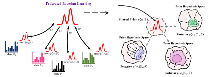
Figure 1: Illustration of the framework of FedABML. On the server side, the global prior $p(\bm{\mathrm{w}}_{i}|\bm{\theta})$ aims to identify the underlying common patterns among heterogeneous clients. On the client side, this prior helps each client effectively accomplish their specific learning tasks $q(\bm{\mathrm{w}}_{i}|\bm{\phi}_{i})\approx p(\bm{\mathrm{w}}_{i}|\mathcal{D}_{i},\bm{\theta})$ with limited training examples and iterations.

Building on these insights, our method provides a flexible and robust framework from a probabilistic perspective. It excels at capturing the uncertainty in personalized parameter estimation, while simultaneously allowing for a clear representation of local diverse knowledge and global common patterns. The incorporation of uncertainty estimates serves as a vital tool in mitigating the impact of overfitting, as it curbs the model’s tendency to become excessively confident in its predictions, thereby enabling well generalization to unseen data. Thus, FedABML empowers the integration of prior knowledge or assumptions regarding the data distribution, which can further enhance the model’s generalization capabilities.

Contributions.

The main contributions of this paper can be summarized as follows:

• We propose a novel perspective on personalized federated learning through Amortized Bayesian Meta-Learning.

• From this perspective, we design a new personalized federated learning algorithm named FedABML, which incorporates a hierarchical variational inference across clients. In this way, the learned global prior identifies common patterns among clients and aids their local tasks without extensive iterations on the client side, while also adapting flexibly to new clients (Section 3).

• We provide a theoretical guarantee for the proposed method. Specifically, we derive an upper bound on the average generalization error across all clients. (Section 4).

• Finally, we conduct extensive experiments on various benchmark tasks to evaluate the empirical performance of FedABML. Our results demonstrate that our method outperforms several competitive baselines. In addition, our method is practical for performing inference with new clients and enables uncertainty quantification (Section 5).

2 Related Work

Federated Learning and challenges.

Recent years have witnessed a growing interest in various aspects of FL. One of the pioneering algorithms in FL is FedAvg (McMahan et al., 2017), which utilizes local SGD updates and server aggregation to construct a shared model from homogeneous client datasets. However, the convergence rate of FedAvg typically deteriorates in the presence of client heterogeneity. In recent years, several variants of FedAvg have been proposed in an attempt to speed up convergence and tackle issues related to heterogeneity (Zhao et al., 2018; Li et al., 2018; Karimireddy et al., 2020; Reddi et al., 2020). For instance, Li et al. (2018) introduced a regularization term in the client objectives, which helps improve the alignment between the local models and the global model. This regularization term contributes to improving the overall performance of the federated learning process. The SCAFFOLD method, proposed by (Karimireddy et al., 2020), introduced control variables and devised improved local training strategies to mitigate client drift. While these methods have made some progress, they tend to prioritize training a single global model for all clients, disregarding the unique demands and preferences of individual clients. This approach overlooks the potential benefits of addressing the unique needs of different clients through personalized models.

Personalised Federated Learning.

Therefore, to maintain the benefits of both federation and personalized models, a variety of recent works have been explored in the context of FL, including clustering (Briggs et al., 2020; Mansour et al., 2020), multi-task learning (Smith et al., 2017; Dinh et al., 2021; Deng et al., 2020), regularized loss functions (T Dinh et al., 2020; Li et al., 2021), transfer learning (Yang et al., 2020; Chen et al., 2020; Razavi-Far et al., 2022), and meta-learning (Chen et al., 2018; Jiang et al., 2019; Fallah et al., 2020; T Dinh et al., 2020). These methods enable the extraction of personalized insights while leveraging the collaborative nature of FL. More recently, a line of work (Chen et al., 2018; Fallah et al., 2020; T Dinh et al., 2020) employed an optimization framework through a Model-Agnostic Meta-Learning (MAML) approach (Finn et al., 2017). Unlike other methods that primarily focus on developing local models during training, these works aimed to initialize a well-performing shared global model that can be further personalized through client-specific updates. With the MAML framework, the global model can be quickly adapted to new clients’ task through inner updates. Recent work by Jiang et al. (2019) studied that the FedAvg algorithm can be viewed as a meta-learning algorithm, where a global model learned through FedAvg can serve as an initial model for each client. Additionally, numerous techniques and algorithms have been proposed for pFL in the face of heterogeneity (see (Tan et al., 2022; Kulkarni et al., 2020) for comprehensive details).

Bayesian Federated Learning.

Bayesian techniques are one of the active areas in machine learning and have been studied for a variety of purposes (Bernardo and Smith, 2009; Wilson and Izmailov, 2020; Garnett, 2023). While standard pFL methods have advanced significantly for heterogeneous client data, they often suffer from model overfitting when data from clients are limited. Bayesian techniques, such as Bayesian neural networks (MacKay, 1992; Neal, 2012; Blundell et al., 2015), which introduce prior distributions on each parameter, can estimate model uncertainty and incorporate prior knowledge to improve generalization performance. This result enables practical FL while preserving the benefits of Bayesian principles (Cao et al., 2023). In particular, it provides a principled way to combine information from multiple clients while accounting for the uncertainty associated with each client’s data. For example, Chen and Chao (2020) employed a novel aggregation method based on Bayesian ensembles at the server’s side, also known as FedBE. FedPA (Al-Shedivat et al., 2020) provided an approximate posterior inference scheme by averaging local posteriors to infer the global posterior. Similarly, the Laplace approximation was introduced by Liu et al. (2021) to approximate posteriors on both the client and server side, which is also known as FOLA. Other variants (such as mixture distribution) (Marfoq et al., 2021) have been investigated under the assumption that local client data distributions can be represented as mixtures of underlying distributions. Another recent approach called pFedbayes (Zhang et al., 2022, 2023b) can be viewed as an implicit regularization-based method that approximates global posteriors from individual posteriors. Guo et al. (2023) showed that the expectation propagation approach can be generalized to FL and attain an accurate approximation to the global posterior distribution. Although the above methods contribute to the understanding of Bayesian FL, none of them fully consider the problem of personalizing FL from the perspective of hierarchical Bayesian.

3 Proposed Method

3.1 Preliminaries

In the conventional conception of FL (McMahan et al., 2017; Reddi et al., 2020) over $N$ clients, we would like to solve the following optimization problem:

$$\min_{\bm{\theta}\in\mathbb{R}^{d}}\,F(\bm{\theta}):=\frac{1}{N}{\sum}_{i=1}^{N}f_{i}(\bm{\theta}),$$ (3.1)

where $F(\bm{\theta})$ is the global loss function, $f_{i}(\bm{\theta}):=\mathbb{E}_{\xi_{i}\sim\mathcal{D}_{i}}[\ell_{i}(\bm{\theta};\xi_{i})]$ corresponds to the expected loss at the $i$ client. We assume that each client $i\in[N]$ holds $n$ training data samples $\xi_{i}$ drawn from the distribution $\mathcal{D}_{i}$. It should be noted that the distributions $\mathcal{D}_{i}$ can vary across clients, which corresponds to client heterogeneity.

Typically, Federated Averaging (FedAvg, McMahan et al. 2017) and its variants are widely used algorithms to solve the traditional FL problem 3.1. However, these approaches only produce a common output for all clients, without adapting the model to each individual client. Consequently, the global model obtained by minimizing 3.1 may not perform well when applied to the local datasets of heterogeneous clients, where each client has a distinct underlying data distribution.

To address this limitation, several FL algorithms have been developed to incorporate personalization into the FL system (Jiang et al., 2019; Fallah et al., 2020; T Dinh et al., 2020). These algorithms aim to modify the formulation of the FL problem in order to leverage the shared information among all clients, enabling each client to obtain a model that is tailored to its specific requirements through fine-tuning. Inspired by the Meta-Learning Finn et al. (2017) approach, a natural idea emerges: to discover an initial point shared among all clients that exhibit good performance when adapted to individual clients through client-specific updates. This idea serves as a guiding principle for several proposed FL algorithms. Concretely,

Per-FedAvg.

With the MAML framework, Per-FedAvg (Fallah et al., 2020) proposes a personalized variant of the FedAvg algorithm and places more emphasis on the initial point which is consensus among clients. Thus, the objective function 3.1 is changed to:

$$\begin{split}\text{Per-FedAvg:}\;\min_{\bm{\theta}\in\mathbb{R}^{d}}\,\Big{\{}F(\bm{\theta}):=\frac{1}{N}{\sum}_{i=1}^{N}f_{i}\big{(}\bm{\mathrm{w}}_{i}(\bm{\theta})\big{)}\Big{\}},\quad\text{where}\;\bm{\mathrm{w}}_{i}(\bm{\theta})=\bm{\theta}-\alpha\nabla f_{i}(\bm{\theta}).\end{split}$$ (3.2)

Based on the MAML framework, 3.2 aims to find a global model $\bm{\theta}$ that can serve as an initialization for each client $i$ to perform an additional gradient update, resulting in a personalized model $\bm{\mathrm{w}}_{i}(\bm{\theta})$. In this way, each client obtains the final model it needs based on the initial model and its own data, where the initial model is obtained collaboratively by all clients in a distributed manner. This approach enables each client to have a model that is tailored to their specific dataset, providing a customized solution.

pFedMe.

Compared to Per-FedAvg, a similar approach is taken by treating $\bm{\theta}$ as a “meta-model”. Specifically, instead of using $\bm{\theta}$ solely as an initialization, pFedMe (T Dinh et al., 2020) introduces a regularized loss function with an $l_{2}$-norm for each client. This is achieved by solving the following bi-level problem:

$$\begin{split}\text{pFedME:}\;\min_{\bm{\theta}\in\mathbb{R}^{d}}\,\Big{\{}F(\bm{\theta}):=\frac{1}{N}{\sum}_{i=1}^{N}F_{i}(\bm{\theta})\Big{\}},\quad\text{where}\;F_{i}(\bm{\theta})=\min_{\bm{\mathrm{w}}_{i}\in\mathbb{R}^{d}}f_{i}(\bm{\mathrm{w}}_{i})+\frac{\lambda}{2}\big{\|}\bm{\mathrm{w}}_{i}-\bm{\theta}\big{\|}^{2},\end{split}$$ (3.3)

where parameter $\bm{\theta}$ is determined by aggregating from multiple clients at the outer level, while the client-specific parameter $\bm{\mathrm{w}}_{i}$ is optimized with respect to the specific data distribution on client $i$. The underlying idea is to allow clients to pursue their own models in different directions while still ensuring that they do not deviate significantly from $\bm{\theta}$, which is a collective representation contributed by all clients.

3.2 Problem Formulation

Typically, $f_{i}(\bm{\theta})$ represents the negative log likelihood of the data $\mathcal{D}_{i}$ on client $i$ under a probabilistic model parameterized by $\bm{\theta}$, i.e., $f_{i}(\bm{\theta}):=-\log p(\mathcal{D}_{i}|\bm{\theta})$. For instance, the least squares loss corresponds to the likelihood under a Gaussian model, while the cross-entropy loss corresponds to categorical distributions. Therefore, the optimization problem 3.1, which aims to find the maximum likelihood estimation (MLE) of the parameters $\bm{\theta}$, can be reformulated from a probabilistic perspective as follows:

$$\begin{split}\min_{\bm{\theta}}\,F(\bm{\theta}):&=-\log p(\mathcal{D}_{1}\cup\dots\cup\mathcal{D}_{N}|\bm{\theta})=\frac{1}{N}{\sum}_{i=1}^{N}-\log p(\mathcal{D}_{i}|\bm{\theta}).\end{split}$$ (3.4)

Upon this, we adopt a different approach by introducing a hierarchical model that consists of a shared global variable $\bm{\theta}$ and client-specific exclusive variables $\bm{\phi}_{i}$ for each client $i$. This hierarchical structure allows for capturing both global patterns shared among all clients and individual characteristics specific to each client. The shared global variable $\bm{\theta}$ represents the common knowledge and information across all clients, while the client-specific variables $\bm{\phi}_{i}$ capture the unique features and nuances of each client’s data. Thus, we employ hierarchical variational inference to lower bound the likelihood of all the data $\mathcal{D}$:

$$-F(\bm{\theta}) =\frac{1}{N}{\sum}_{i=1}^{N}\log p(\mathcal{D}_{i}|\bm{\theta})=\frac{1}{N}{\sum}_{i=1}^{N}\log\int p(\mathcal{D}_{i}|\bm{\mathrm{w}}_{i})\,p(\bm{\mathrm{w}}_{i}|\bm{\theta})d\bm{\mathrm{w}}_{i}$$

$$\geq\frac{1}{N}{\sum}_{i=1}^{N}\int q(\bm{\mathrm{w}}_{i}|\bm{\phi}_{i})\Big{[}\log p(\mathcal{D}_{i}|\bm{\mathrm{w}}_{i})-\log\frac{q(\bm{\mathrm{w}}_{i}|\bm{\phi}_{i})}{p(\bm{\mathrm{w}}_{i}|\bm{\theta})}\Big{]}d\bm{\mathrm{w}}_{i}$$

$$=\frac{1}{N}\sum_{i=1}^{N}\mathbb{E}_{q(\bm{\mathrm{w}}_{i}|\bm{\phi}_{i})}[\log p(\mathcal{D}_{i}|\bm{\mathrm{w}}_{i})]-\mathrm{KL}[q(\bm{\mathrm{w}}_{i}|\bm{\phi}_{i})\|p(\bm{\mathrm{w}}_{i}|\bm{\theta})],$$

where $\mathbb{E}_{q(\bm{\mathrm{w}}_{i}|\bm{\phi}_{i})}[\log p(\mathcal{D}_{i}|\bm{\mathrm{w}}_{i})]-\mathrm{KL}[q(\bm{\mathrm{w}}_{i}|\bm{\phi}_{i})\|p(\bm{\mathrm{w}}_{i}|\bm{\theta}]$ is often known as the Evidence Lower Bound (ELBO) associated with the local data $\mathcal{D}_{i}$, the $\mathrm{KL}$ is the Kullback-Leibler divergence which serves as a regularization and penalizes the difference between the global prior $p(\bm{\mathrm{w}}_{i}|\bm{\theta})$ and the local approximated posterior $q(\bm{\mathrm{w}}_{i}|\bm{\phi}_{i})$. The first term of ELBO is commonly referred to as the likelihood cost.

Building upon this intuition, we introduce a novel and general FL algorithm in this paper, called FedABML. We extend the previous work (Fallah et al., 2020; T Dinh et al., 2020), and propose a hierarchical variational meta-learning approach for personalized FL. In particular, the optimization of negative Federated Evidence Lower Bound (Fed-ELBO) can be formulated as a bi-level problem:

$$\begin{split}\min_{\bm{\theta}}\;F(\bm{\theta}&)=\frac{1}{N}{\sum}_{i=1}^{N}f_{i}(\bm{\theta})\\ \operatorname{s.t.}\;f_{i}(\bm{\theta})&=\min_{\bm{\phi}_{i}}\,\Big{\{}\mathbb{E}_{q(\bm{\mathrm{w}}_{i}|\bm{\phi}_{i})}\big{[}-\log p(\mathcal{D}_{i}|\bm{\mathrm{w}}_{i})\big{]}+\mathrm{KL}\big{[}q(\bm{\mathrm{w}}_{i}|\bm{\phi}_{i})\|p(\bm{\mathrm{w}}_{i}|\bm{\theta})\big{]}\Big{\}}\\ &=\min_{\bm{\phi}_{i}}\,\mathrm{KL}\big{[}q(\bm{\mathrm{w}}_{i}|\bm{\phi}_{i})\|p(\bm{\mathrm{w}}_{i}|\mathcal{D}_{i},\bm{\theta})\big{]},\end{split}$$ (3.5)

where $\bm{\theta}$ denotes the global prior parameters that aim to capture shared statistical structure across all clients. Each client-specific $\bm{\phi}_{i}$ represents the variational parameters of the local approximate posteriors $q(\bm{\mathrm{w}}_{i}|\bm{\phi}_{i})\approx p(\bm{\mathrm{w}}_{i}|\mathcal{D}_{i},\bm{\theta})$, which are able to align with their respective data distribution. Furthermore, $\bm{\mathrm{w}}_{i}$ corresponds to the weights of a deep neural network, while $\bm{\theta}$ and $\bm{\phi}_{i}$ denote the parameters and variational parameters of the weight distribution, such as a mean and standard deviation of each weight.

From 3.5, we observe that the global prior $p(\bm{\mathrm{w}}_{i}|\bm{\theta})$ serves the purpose of identifying the shared common patterns among a set of clients. This prior helps each client effectively accomplish their respective learning tasks with only a small number of training examples and iterations. To this end, our learning procedure consists of two distinct steps. In the first step, sever learn the shared prior parameters $\bm{\theta}^{\star}$ through exploiting the data aggregation across multiple clients: $\bm{\theta}_{i}^{\star}=\arg\min_{\bm{\theta}_{i}}\frac{1}{N}\sum_{i}\mathbb{E}_{q(\bm{\mathrm{w}}_{i}|\bm{\phi}_{i})}[-\log p(\mathcal{D}_{i}|\bm{\mathrm{w}}_{i})]+\mathrm{KL}[q(\bm{\mathrm{w}}_{i}|\bm{\phi}_{i})\|p(\bm{\mathrm{w}}_{i}|\bm{\theta})]$. The resulting $\bm{\theta}^{\star}$ can be viewed as common knowledge among heterogeneous clients. In the second step, using $p(\bm{\mathrm{w}}_{i}|\bm{\theta}^{\star})$ as the prior, we aim to obtain client-specific variational posterior parameters $\bm{\phi}^{\star}$ that can effectively generalize well on their own data $\mathcal{D}_{i}$ after a few trials: $\bm{\phi}_{i}^{\star}=\arg\min_{\bm{\phi}_{i}}\mathrm{KL}[q(\bm{\mathrm{w}}_{i}|\bm{\phi}_{i})\|p(\bm{\mathrm{w}}_{i}|\mathcal{D}_{i},\bm{\theta})]$. The client-specific variational parameters $\bm{\phi}_{i}^{\star}$ can be viewed as transferred knowledge derived from the shared information among a collection of clients. In addition, a constraint $\mathrm{KL}[q(\bm{\mathrm{w}}_{i}|\bm{\phi}_{i})\|p(\bm{\mathrm{w}}_{i}|\bm{\theta})]$ is in place to ensure that these posteriors should not be far from the “reference prior distribution” $p(\bm{\mathrm{w}}_{i}|\bm{\theta})$.

Before proceeding further, we are interested in the connection with some meta-learning based methods mentioned before. Specifically,

Remark (Relation to Per-FedAvg).

For comparison, we consider the simplest case, where both the approximate posterior and prior are assumed to be the Dirac delta function:

$$q(\bm{\mathrm{w}}_{i}|\bm{\phi}_{i})=\delta(\bm{\mathrm{w}}_{i}-\bm{\mathrm{w}}_{i}^{\text{MAP}}),\quad p(\bm{\mathrm{w}}_{i}|\bm{\theta})=\delta(\bm{\mathrm{w}}_{i}-\bm{\theta}),$$

where the local mode $\bm{\mathrm{w}}_{i}^{\text{MAP}}$ can be obtained by using maximum a posterior. Then, gradient descent is used, and the local mode can be determined as:

$$\bm{\mathrm{w}}_{i}^{\text{MAP}} =\arg\max_{\bm{\mathrm{w}}_{i}}\big{[}\log p(\mathcal{D}_{i}|\bm{\mathrm{w}}_{i})+\log p(\bm{\mathrm{w}}_{i}|\bm{\theta})\big{]}$$

$$\approx\bm{\theta}-\eta_{\alpha}\nabla_{\bm{\mathrm{w}}_{i}}\big{[}-\log p(\mathcal{D}_{i}|\bm{\mathrm{w}}_{i})\big{]}\big{|}_{\bm{\mathrm{w}}_{i}=\theta}.$$

Based on this, our method can be formulated as follows:

$$\min_{\bm{\theta}}\;f(\bm{\theta}):=\frac{1}{N}{\sum}_{i=1}^{N}f_{i}\big{(}\bm{\phi}_{i}(\bm{\theta})\big{)},\quad\operatorname{s.t.}\;\bm{\phi}_{i}\big{(}\bm{\theta}\big{)}=\bm{\theta}-\alpha\nabla_{\bm{\mathrm{w}}_{i}}\big{[}-\log p(\mathcal{D}_{i}|\bm{\mathrm{w}}_{i})\big{]}\big{|}_{\bm{\mathrm{w}}_{i}=\theta}.$$ (3.6)

Compared to 3.2, Per-FedAvg can be viewed as a special case of our method where all distributions reduce to point estimates.

Remark (Relation to pFedMe).

Compared to pFedMe, our problem has a similar meaning of $\bm{\theta}$ as a “meta-model”, but instead of using $\bm{\theta}$ as the single “reference point”. Moreover, let $p(\bm{\mathrm{w}}_{i}|\bm{\theta})=\mathcal{N}(\bm{\mathrm{w}}_{i}|\bm{\theta},I/\lambda)$, $q(\bm{\mathrm{w}}_{i}|\bm{\phi}_{i})=\mathcal{N}(\bm{\mathrm{w}}_{i}|\bm{\phi}_{i},I/\rho)$. Next, rewriting the 3.5 as:

$$\min_{\bm{\theta}}\;F(\bm{\theta}):=\frac{1}{N}{\sum}_{i=1}^{N}F_{i}(\bm{\theta}),\quad\operatorname{s.t.}\;F_{i}(\bm{\theta})=\min_{\bm{\phi}_{i}}\mathbb{E}_{q(\bm{\mathrm{w}}_{i}|\bm{\phi}_{i})}\big{[}-\log(\mathcal{D}_{i}|\bm{\mathrm{w}}_{i})\big{]}+\frac{\lambda}{2}\big{\|}\bm{\phi}_{i}-\bm{\theta}\big{\|}^{2}.$$ (3.7)

The results show that our method is a relaxation of pFedMe, which arguably has a close idea to pFedMe. In addition, $\lambda$ plays the exact same role as a regularization tuning parameter.

3.3 Algorithm

With the objective 3.5 in mind, we now detail how to implement a specific model. We first outline the distribution forms of the priors and posteriors.

Distribution of global prior $p(\bm{\mathrm{w}}_{i}|\bm{\theta})$.

The global prior distribution is assumed to be a multivariate Gaussian distribution with parameters $\bm{\theta}=\big{\{}\bm{m}_{\theta},\bm{\Lambda}_{\theta}\big{\}}$. Then, the shared prior distribution for client $i$ to be:

$$p\big{(}\bm{\mathrm{w}}_{i}|\bm{\theta}\big{)}=\mathcal{N}\big{(}\bm{\mathrm{w}}_{i}|\bm{m}_{\bm{\theta}},\bm{\Lambda}_{\bm{\theta}}\big{)},$$

which is a Gaussian distribution with mean vector $\bm{m}_{\theta}\in\mathbb{R}^{d}$ and a diagonal covariance matrix $\bm{\Lambda}_{\theta}={\bm{\sigma}}_{\bm{\theta}}^{2}I_{d}\in\mathbb{R}^{d\times d}$.

Distribution of approximated local posterior $q(\bm{\mathrm{w}}_{i}|\bm{\phi}_{i})$.

For $q\big{(}\bm{\mathrm{w}}_{i}|\bm{\phi}_{i}\big{)}$, $\bm{\mathrm{w}}_{i}$ denotes the weights of a deep neural network and $\bm{\phi}_{i}$ denotes the variational parameters (i.e., means and standard deviations). Due to the high dimension of $\bm{\mathrm{w}}_{i}$, it is computationally difficult to learn variational parameters $\bm{\phi}_{i}$. Hence, we resort to amortized variational inference (Ravi and Beatson, 2019; Ganguly et al., 2022),

$$q\big{(}\bm{\mathrm{w}}_{i}|\bm{\phi}_{i}\big{)}\approx q\big{(}\bm{\mathrm{w}}_{i}|\bm{\theta},\mathcal{D}_{i};\bm{\phi}_{i}\big{)}:=q\big{(}\bm{\mathrm{w}}_{i};{SGD}_{k}(\bm{\theta},\mathcal{D}_{i},\eta)\big{)}.$$

From a global initialization $\bm{\theta}$, we produce the variational parameter $\bm{\phi}_{i}$ by conducting several steps of gradient descent. Let $\mathcal{L}_{i}(\bm{\theta},\bm{\phi}_{i})=\mathbb{E}_{q(\bm{\mathrm{w}}_{i}|\bm{\phi}_{i})}[-\log p(\mathcal{D}_{i}|\bm{\mathrm{w}}_{i})]+\mathrm{KL}[q(\bm{\mathrm{w}}_{i}|\bm{\phi}_{i})\|p(\bm{\mathrm{w}}_{i}|\bm{\theta})]$ be the loss on the client $\mathcal{D}_{i}$. We define the procedure of stochastic gradient descent, ${SGD}_{k}(\bm{\theta},\mathcal{D}_{i},\eta)$, to produce $\bm{\phi}_{i}$ from the global initialization $\bm{\theta}$:

$$\begin{split}1.\ &\bm{\phi}_{i}^{0}\leftarrow\bm{\theta}.\\ 2.\ &\text{for }\kappa=0,\cdots,k-1,\text{set}\\ &\quad\bm{\phi}_{i}^{\kappa}\leftarrow\bm{\phi}_{i}^{\kappa-1}-\eta\nabla_{\bm{\phi}_{i}}\mathcal{L}_{i}(\bm{\theta},\bm{\phi}_{i}^{\kappa-1}),\\ \end{split}$$ (3.8)

where $k$ is the gradient descent steps and $\eta$ is the learning rate.

Reparameterization Trick.

With well-defined prior $p(\bm{\mathrm{w}}_{i}|\bm{\theta})$ and the posterior $q(\bm{\mathrm{w}}_{i}|\bm{\phi}_{i})$, solving equation 3.5 by Monte Carlo sampling is a straightforward process. The reparameterization trick (Blundell et al., 2015; Kingma et al., 2015) provides a computationally and statistically efficient method for estimating gradients, which helps improve numerical stability. Specifically, we parameterize the standard deviation point-wisely as $\bm{\sigma}=\exp(\bm{\nu})$ when performing gradient update for the standard deviations of model parameters. In this way, the global prior parameters and the variational posterior parameters can be rewritten as $\bm{\theta}=\big{\{}\bm{m}_{\bm{\theta}},\exp(\bm{\nu}_{\bm{\theta}})\big{\}}$ and $\bm{\phi}_{i}=\big{\{}\bm{m}_{i},\exp(\bm{\nu}_{i})\big{\}}$. Thus, we can update the variational distribution $\bm{\phi}_{i}$ can be updated by minimizing the local negative EBLO in 3.5 with stochastic backpropagation and the reparameterization trick:

$$\bm{\mathrm{w}}_{i}\mid\bm{\phi}_{i}=\bm{m}_{i}+\epsilon\circ\exp(\bm{\nu}_{i}),$$ (3.9)

where $\epsilon\sim\mathcal{N}(0,I_{d})$, and $\circ$ denotes the element-wise multiplication. Given this direct dependency, the gradients of the cost function $\mathcal{L}_{i}(\bm{\phi}_{i},\bm{\theta})$ in 3.5 with respect to $\bm{\phi}_{i}$ can be derived as:

$$\begin{split}\nabla_{\bm{m}_{i}}\mathcal{L}_{i}&=\frac{\partial\mathcal{L}_{i}(\bm{\theta},\bm{\phi}_{i})}{\partial\bm{\mathrm{w}}_{i}}+\frac{\partial\mathcal{L}_{i}(\bm{\theta},\bm{\phi}_{i})}{\partial\bm{m}_{i}},\\ \nabla_{\bm{\nu}_{i}}\mathcal{L}_{i}&=\frac{\partial\mathcal{L}_{i}(\bm{\theta},\bm{\phi}_{i})}{\partial\bm{\mathrm{w}}_{i}}\epsilon\circ\exp(\bm{\nu}_{i})+\frac{\partial\mathcal{L}_{i}(\bm{\theta},\bm{\phi}_{i})}{\partial\bm{\nu}_{i}}.\end{split}$$ (3.10)

The training process of our FedABML is summarized in Algorithm 1. In each round of FedABML, the server selects a fraction of clients with size $\tau N$ ($\tau\in(0,1])$ and sends its current prior parameters $\bm{\theta}_{t}$ to these clients (Line 4). During the client update stage, each selected client updates its approximated posterior $q(\bm{\mathrm{w}}_{i}|\bm{\phi}_{i})$ by utilizing its own data distribution $\mathcal{D}_{i}$ and performing $k\geq 1$ steps of stochastic gradient descent (Line 8). Then, each client updates the global prior $p(\bm{\mathrm{w}}_{i}|\bm{\theta}_{t})$ based on the performance of its updated posterior (Line 9). Finally, the server averages the updates received from these sampled clients and then proceeds to the next round (Line 10).

Algorithm 1 Personalized Federated Learning via Amortized Bayesian Meta-Learning (FedABML)

1:  Input: Initial iterate $\bm{\theta}_{0}$, fraction of active clients $\tau$, learning rates $\eta,\eta^{\prime}$, $T$, $R$.

2:  for $t=0$ to $T-1$ do

3:     Server chooses a subset of clients $\mathcal{A}_{t}$ uniformly at random; $\triangleright$ Global communication rounds

4:     Server sends $\bm{\theta}_{t}$ to all clients in $\mathcal{A}_{t}$;

5:     for all $i\in\mathcal{A}_{t}$ do

6:        $\bm{\phi}_{i,0}^{t}\leftarrow\bm{\theta}_{t};\quad\bm{\theta}_{i,0}^{t}\leftarrow\bm{\theta}_{t}$ $\triangleright$ Local update rounds

7:        for $r=0$ to $R-1$ do

8:           draw $s$ samples $\bm{\mathrm{w}}_{i}\sim q(\bm{\mathrm{w}}_{i}|\bm{\phi}_{i,r}^{t})$ and update

$$\bm{\phi}_{i,r+1}^{t}\leftarrow\bm{\phi}_{i,r}^{t}-\eta\nabla_{\bm{\phi}}\mathcal{L}_{i}(\bm{\phi}_{i,r}^{t},\bm{\theta}_{i,r}^{t})$$

9:           dram $s$ samples $\bm{\mathrm{w}}_{i}\sim q(\bm{\mathrm{w}}_{i}|\bm{\phi}_{i,r+1}^{t})$ and update

$$\bm{\theta}_{i,r+1}^{t}\leftarrow\bm{\theta}_{i,r}^{t}-\eta^{\prime}\nabla_{\bm{\theta}}\mathcal{L}_{i}(\bm{\phi}_{i,r+1}^{t},\bm{\theta}_{i,r}^{t})$$

10:     Server updates: $\bm{\theta}_{t+1}\leftarrow\frac{1}{|\mathcal{A}_{t}|}\sum_{i\in\mathcal{A}_{t}}\bm{\theta}_{i,R}^{t}$

4 Theoretical Results

In this section, we present the theoretical analysis of our method. We start with the regression-based data modeling perspective and introduce some related assumptions and notations necessary for the proof of our theoretical results. Let us consider the $i$-th client, which satisfies a nonparametric regression model with random covariates:

$$y_{i}^{(m)} =f_{i}(\mathrm{x}_{i}^{(m)})+\varepsilon_{i}^{(m)},\;\varepsilon_{i}^{(m)}\sim\mathcal{N}(0,\sigma_{\varepsilon}^{2}),\quad m=1,\ldots,n,$$

where the data is a random data sample drawn from the distribution of client $i$, denoted as $(\mathrm{x}_{i}^{(m)},y_{i}^{(m)})\sim\mathcal{D}_{i},i=1,\dots,N$. The target variable $y_{i}^{(m)}\in\mathbb{R}^{\mathcal{Y}}$ is real vector, and each client $i$ has a true regression function $f_{i}:\,\mathbb{R}^{\mathcal{X}}\rightarrow\mathbb{R}^{\mathcal{Y}}$. For simplicity of analysis, we assume that the noise variance $\sigma_{\varepsilon}$ for all clients is the same, and the number of data points is the same for each client $|\mathcal{D}_{i}|=n$.

Recall that each client employs the same neural network architecture, i.e., a fully-connected Deep Neural Network (DNN). However, due to the non-i.i.d. nature of their respective datasets, the parameters of the DNN vary across clients. Specifically, a neural network consists $L$ hidden layers, with the $l$-th layer having $s_{l}$ neurons and activation functions $\sigma(\cdot)$ for $l=0,1,...,L$. As a consequence, the weight matrix and bias parameters for each layer are denoted as $W_{l}\in\mathbb{R}^{s_{l}\times s_{l+1}}$ and $b_{l}\in\mathbb{R}^{s_{l+1}}$ for $l=0,\ldots,L$. Then, given parameters $\mathrm{w}=$ $\big{\{}W_{0},b_{0},\dots,W_{L-1},b_{L-1},W_{L},b_{L}\big{\}}$, the output of the DNN model can be represented as:

$$f_{\bm{\mathrm{w}}}(\mathrm{x})=W_{L}\sigma\big{(}W_{L-1}\sigma(\dots\sigma(W_{0}\mathrm{x}+b_{0})\dots)+b_{L-1}\big{)}+b_{L}.$$

Before proceeding further, we introduce additional notations to simplify the exposition and analysis throughout this section. Let $f(\mathrm{X}_{i})$ denote the concatenated vector of $f(\mathrm{x})$ for all $\mathrm{x}\in\mathrm{X}_{i}$ , i.e., $f(\mathrm{X}_{i})=[f(\mathrm{x})]_{\mathrm{x}\in\mathrm{X}_{i}}$, where $f(\cdot)$ refers to either the true $f_{i}(\cdot)$ or the model $f_{\bm{\mathrm{w}}_{i}}(\cdot)$ for the $i$-th client. Furthermore, let $P_{0}$ denote the underlying probability measure of the data, and $p_{0}$ represent the corresponding density function, i.e., $p_{0}=\mathcal{N}(f_{0}(\mathrm{x}_{i}),\sigma^{2}_{\varepsilon})$.

For simplicity, we analyze the equal-width neural network, as done in previous works such as Polson and Ročková (2018); Bai et al. (2020).

Assumption 1.

In our FL model, we state the following assumptions throughout the paper.

• The backbone network is a neural network with $L$-hidden-layers, and each layer has equal width $M$ ($s_{l}=M,l=1,\dots,L$). The parameters $\mathrm{w}$ of the backbone network are also assumed to be bounded. More formally,

  $$\bm{\mathrm{w}}\in\mathbb{W}=\{\bm{\mathrm{w}}\in\mathbb{R}^{d}:\|\bm{\mathrm{w}}\|_{\infty}\leq B\}.$$

• Additionally, all activation functions $\sigma(\cdot)$ are assumed to be $1$-Lipschitz continuous (e.g., ReLU, sigmoid and tanh).

Next, recall the definition of generalized Hellinger divergence, which plays a crucial role in the analysis of our method. As a measure of the generalization error, we consider the expected squared Hellinger distance between the true distribution $P_{i}$ and the model distribution $P_{\bm{\mathrm{w}}}$. Formally,

Definition 1 (Hellinger Distance).

For probability measures $P_{\bm{\mathrm{w}}}$ and $P_{i}$, the Hellinger distance between them is defined as

$$d^{2}(P_{\bm{\mathrm{w}}},P_{i})=\mathbb{E}_{\mathrm{x}\sim p_{i}(\mathrm{x})}\big{[}1-\exp\big{(}-{\big{\|}f_{\bm{\mathrm{w}}}(\mathrm{x})-f_{i}(\mathrm{x})\big{\|}_{2}^{2}}/{(8\sigma_{\epsilon}^{2})}\big{)}\big{]}.$$

4.1 Main Theorem

More specifically, we will bound the posterior-averaged distance $\frac{1}{N}{\sum}_{i=1}^{N}\mathbb{E}_{q^{\star}(\bm{\mathrm{w}}_{i}|\bm{\phi}_{i})}\big{[}d^{2}\big{(}P_{\bm{\mathrm{w}}_{i}},P_{i}\big{)}\big{]}$, where $q^{\star}(\bm{\mathrm{w}}_{i}|\bm{\phi}_{i})$ is an optimal solution of our negative Fed-ELBO objective (3.5).

Theorem 1 (Generalization bound).

Assuming Assumption 1, then we have the following upper bound holds (with high probability):

$$\begin{split}\frac{1}{N}{\sum}_{i=1}^{N}\mathbb{E}_{q^{\star}(\bm{\mathrm{w}}_{i}|\bm{\phi}_{i})}&\big{[}d^{2}\big{(}P_{\bm{\mathrm{w}}_{i}},P_{i}\big{)}\big{]}\leq C\epsilon_{n}^{2}+C^{\prime}r_{n}+C^{\prime\prime}\frac{1}{N}{\sum}_{i=1}^{N}\xi_{i},\end{split}$$ (4.1)

where $C,C^{\prime},C^{\prime\prime}>0$ are some positive constant, $\xi_{i}=\inf_{\bm{\mathrm{w}}_{i}\in\mathbb{W}}\big{\|}f_{\bm{\mathrm{w}}_{i}}-f_{i}\big{\|}_{\infty}^{2}$ is the best error within our backbone $\mathbb{W}$, $r_{n}=({(L+1)}d/{n})\log M+(d/n)\log(s_{0}\sqrt{n/d})$ and $\epsilon_{n}=\sqrt{r_{n}}\log^{\delta}(n)$ for $\delta>1$ constant.

Remark.

Given that the former two errors have only logarithmic difference, the upper bound 4.1 can be divided into two parts: the first and second terms correspond to the estimation error (i.e., $\varepsilon_{n}^{2}$, $r_{n}$), while the third term represents the approximation error (i.e., $\xi_{i}$). This is easy to verify: the estimation error decreases with the increase of sample size as $n\rightarrow\infty$, $r_{n}\rightarrow 0$ obviously, accordingly $\epsilon_{n}\rightarrow 0$. On the other hand, the approximation error $\xi_{i}$ depends on the total number of parameters $T$ (width and depth) of the neural network. As the number of parameters increases (larger $T$), the approximation error decreases, while the estimation error increases. The convergence rate achieved by our method strikes a balance among these three error terms, taking into account the sample size, model complexity, and approximation error. Consequently, Theorem 1 implies the optimal solution for our negative Fed-ELBO problem 3.5 is asymptotically optimal.

4.2 Proof Sketch

In this subsection, we demonstrate our proof framework by sketching the proof for Theorem 1. The proof of Theorem 1 is based on the following two lemmas regarding the convergence of the variational distribution under the Hellinger distance and an upper bound for the negative Fed-ELBO respectively. For simplicity, we will write the following symbols $q(\bm{\mathrm{w}}_{i}):=q(\bm{\mathrm{w}}_{i}|\bm{\phi}_{i}),\,p(\bm{\mathrm{w}}_{i})=p(\bm{\mathrm{w}}_{i}|\theta)$.

Lemma 2.

Assuming Assumption 1, the following inequality holds (with dominating probability) for some constant $C>0$:

$$\begin{split}&\frac{1}{N}{\sum}_{i=1}^{N}\mathbb{E}_{q(\bm{\mathrm{w}}_{i})}\big{[}d^{2}(P_{\bm{\mathrm{w}}_{i}},P_{i})\big{]}\leq C\varepsilon_{n}^{2}+\frac{1}{n}\Big{\{}\frac{1}{N}{\sum}_{i=1}^{N}\mathbb{E}_{q(\bm{\mathrm{w}}_{i})}\big{[}\ell_{n}(P_{\bm{\mathrm{w}}_{i}},P_{i})\big{]}+\mathrm{KL}\big{(}q(\bm{\mathrm{w}}_{i})\|p(\bm{\mathrm{w}}_{i}|\theta)\big{)}\Big{\}}\end{split}$$ (4.2)

where $\epsilon_{n}=\sqrt{r_{n}}\log^{\delta}(n)$ for any $\delta>1$ and $\ell_{n}\big{(}P_{\bm{\mathrm{w}}_{i}},P_{i}\big{)}:=-\log p({\mathcal{D}_{i}|\bm{\mathrm{w}}_{i}})/\log p_{i}(\mathcal{D}_{i})$.

Lemma 3.

Assuming Assumption 1, then with dominating probability, the following inequality holds for some constant $C^{\prime},C^{\prime\prime}>0$:

$$\begin{split}&\frac{1}{N}{\sum}_{i=1}^{N}\Big{\{}\mathbb{E}_{q(\bm{\mathrm{w}}_{i})}\big{[}\ell_{n}(P_{\bm{\mathrm{w}}_{i}},P_{i})\big{]}+\mathrm{KL}\big{(}q(\bm{\mathrm{w}}_{i})\|p(\bm{\mathrm{w}}_{i}|\theta)\big{)}\Big{\}}\leq n\big{(}C^{\prime}r_{n}+C^{\prime\prime}\frac{1}{N}{\sum}_{i=1}^{N}\xi_{i}\big{)},\end{split}$$ (4.3)

where $r_{n}=({(L+1)}d/{n})\log M+(d/n)\log(s_{0}\sqrt{n/d})$ and $\xi_{i}=\inf_{\bm{\mathrm{w}}_{i}\in\mathbb{W}}\|f_{\bm{\mathrm{w}}_{i}}-f_{i}\|_{\infty}^{2}.$

The proof of Lemmas 2 and 3 is deferred to Section 4.3. With Lemmas 2 and 3 at hands, the proof of Theorem 1 is immediate.

Proof of Theorem 1.

Combining 4.2 and 4.3 yields

$$\frac{1}{N}{\sum}_{i=1}^{N}\mathbb{E}_{q(\bm{\mathrm{w}}_{i})}[d^{2}(P_{\bm{\mathrm{w}}_{i}},P_{i})]\leq\frac{1}{n}nC^{\prime}\big{(}r_{n}+\xi_{i}\big{)}+C\varepsilon_{n}^{2}\leq C^{\prime}\big{(}r_{n}+\xi_{i}\big{)}+C\varepsilon_{n}^{2}.$$

∎

4.3 Proof of Lemmas

4.3.1 Deferred Proof of Lemma 2

Proof of Lemma 2.

Applying Lemma 4 with the specified $q(z):=q(\bm{\mathrm{w}}_{i}),p(z):=p(\bm{\mathrm{w}}_{i}|\bm{\theta})$ and $h(z):=\log\eta(P_{\bm{\mathrm{w}}_{i}},P_{i})$ yields (for any $\bm{\theta}$)

$$\log\mathbb{E}_{p(\bm{\mathrm{w}}_{i}|\bm{\theta})}\big{[}\eta(P_{\bm{\mathrm{w}}_{i}},P_{i})\big{]}\geq\mathbb{E}_{q(\bm{\mathrm{w}}_{i})}\big{[}\log\eta(P_{\bm{\mathrm{w}}_{i}},P_{i})\big{]}-\mathrm{KL}\big{(}q(\bm{\mathrm{w}}_{i})\|p(\bm{\mathrm{w}}_{i}|\theta)\big{)},$$

where $\eta(P_{\bm{\mathrm{w}}_{i}},P_{i}):=\exp\{-\ell_{n}\big{(}P_{\bm{\mathrm{w}}_{i}},P_{i}\big{)}+nd^{2}(P_{\bm{\mathrm{w}}_{i}},P_{i})\}$ and $\ell_{n}\big{(}P_{\bm{\mathrm{w}}_{i}},P_{i}\big{)}:=-\log p({\mathcal{D}_{i}|\bm{\mathrm{w}}_{i}})/\log p_{i}(\mathcal{D}_{i})$.

Dividing both sides by $n$ and rearranging

$$\mathbb{E}_{q(\bm{\mathrm{w}}_{i})}\big{[}d^{2}(P_{\bm{\mathrm{w}}_{i}},P_{i})\big{]}\leq\frac{1}{n}\Big{\{}\mathbb{E}_{q(\bm{\mathrm{w}}_{i})}\big{[}\ell_{n}(P_{\bm{\mathrm{w}}_{i}},P_{i})\big{]}+\mathrm{KL}\big{(}q(\bm{\mathrm{w}}_{i})\|p(\bm{\mathrm{w}}_{i}|\theta)\big{)}\Big{\}}+C\varepsilon^{2}_{n},$$

where the last inequality is due to $\mathbb{E}_{p(\mathrm{w})}[\eta(\mathrm{w})]\leq e^{Cn\varepsilon^{2}_{n}}$ from the Theorem 3.1 in (Pati et al., 2018).

Taking average over $i=1,\dots,N$ gives (the average over clients)

$$\frac{1}{N}{\sum}_{i=1}^{N}\mathbb{E}_{q(\bm{\mathrm{w}}_{i})}\big{[}d^{2}(P_{\bm{\mathrm{w}}_{i}},P_{i})\big{]}\leq C\varepsilon^{2}_{n}+\frac{1}{nN}{\sum}_{i=1}^{N}\Big{\{}\mathbb{E}_{q(\bm{\mathrm{w}}_{i})}\big{[}\ell_{n}(P_{\bm{\mathrm{w}}_{i}},P_{i})\big{]}+\mathrm{KL}\big{(}q(\bm{\mathrm{w}}_{i})\|p(\bm{\mathrm{w}}_{i}|\theta)\big{)}\Big{\}},$$

completing the proof of Lemma 2. ∎

4.3.2 Deferred Proof of Lemma 3

Proof of Lemma 3.

We start by analyzing $\mathrm{KL}(q(\bm{\mathrm{w}}_{i})\|p(\bm{\mathrm{w}}_{i}|\theta))$ in the inequality of Lemma 3: It suffices to construct some $q^{\star}(\bm{\mathrm{w}})\in\mathbb{W}$, such that w.h.p,

$$\mathbb{E}_{q^{\star}(\bm{\mathrm{w}}_{i})}\big{[}\ell_{n}(P_{\bm{\mathrm{w}}_{i}},P_{i})\big{]}+\mathrm{KL}\big{(}q^{\star}(\bm{\mathrm{w}}_{i})\|p(\bm{\mathrm{w}}_{i}|\theta)\big{)}\leq nC_{0}^{\prime}\big{(}r_{n}+\xi_{i}\big{)}.$$

Recall $\bm{\mathrm{w}}_{i}^{\star}=\arg\min_{\bm{\mathrm{w}}_{i}\in\mathbb{W}}\|f_{\bm{\mathrm{w}}_{i}}-f_{i}\|^{2}_{2}$, then $q^{\star}(\bm{\mathrm{w}})$ can be constructed as

$$\mathrm{KL}\big{(}q^{\star}(\bm{\mathrm{w}}_{i})\|p(\bm{\mathrm{w}}_{i}|\theta)\big{)}\leq C^{\prime}_{0}nr_{n},\text{and}\;\mathbb{E}_{q^{\star}(\bm{\mathrm{w}}_{i})}\|f_{\bm{\mathrm{w}}_{i}}-f_{\bm{\mathrm{w}}_{i}^{\star}}\|_{\infty}^{2}\leq r_{n}.$$

Then, the $q^{\star}(\bm{\mathrm{w}}_{i})$ can be defined as : $\bm{\mathrm{w}}\sim\mathcal{N}(\bm{\mathrm{w}}^{\star},\sigma^{2}_{n}),$ where $\sigma_{n}^{2}=\nicefrac{{d}}{{8n}}\cdot A\leq B^{2},$ and $A^{-1}=\log(3s_{0}M)\cdot(2BM)^{2(L+1)}\big{[}(s_{0}+1+\nicefrac{{1}}{{BM-1}})^{2}+\nicefrac{{1}}{{(2BM)^{2}-1}}+\nicefrac{{2}}{{(2BM-1)^{2}}}\big{]}.$ Thus,

$$\mathrm{KL}\big{(}q(\bm{\mathrm{w}}_{i})\|p(\bm{\mathrm{w}}_{i}|\theta)\big{)}\leq\nicefrac{{d}}{{2}}\log\big{(}\nicefrac{{2B^{2}}}{{\sigma_{n}^{2}}}\big{)}$$ (by the Proof of Lemma 2 in (Zhang et al., 2022))

$$\leq d(L+1)\log(2BM)+\nicefrac{{d}}{{2}}\log(3s_{0}M)+d\log\big{(}4s_{0}\sqrt{\nicefrac{{n}}{{d}}}\big{)}+\nicefrac{{d}}{{2}}\log(2B^{2}) \sigma_{n}^{2}$$ (definition of )

$$\leq C_{0}^{\prime}nr_{n}.$$

Consequently, taking average over $i=1,\dots,N$ gives

$$\frac{1}{N}{\sum}_{i=1}^{N}\mathrm{KL}\big{(}q^{\star}(\bm{\mathrm{w}}_{i})\|p(\bm{\mathrm{w}}_{i}|\theta)\big{)}\leq C_{0}^{\prime}nr_{n},$$ (4.4)

and the $\mathrm{KL}$ term on 4.3 is bounded. Furthermore, by Appendix in (Chérief-Abdellatif, 2020), it can be shown

$$\mathbb{E}_{q(\bm{\mathrm{w}}_{i})}\big{[}\big{\|}f_{\bm{\mathrm{w}}_{i}}-f_{\bm{\mathrm{w}}_{i}^{\star}}\big{\|}_{\infty}^{2}\big{]}\leq\nicefrac{{s_{0}}}{{n}}\leq r_{n}.$$ (4.5)

It remains to investigate the first term in the inequality of Lemma 3. From our regression model assumption,

$$\mathbb{E}_{q(\bm{\mathrm{w}}_{i})}\big{[}\ell_{n}\big{(}P_{\bm{\mathrm{w}}_{i}},P_{i}\big{)}\big{]}$$

$$=\mathbb{E}_{q(\bm{\mathrm{w}}_{i})}\big{[}\log p_{i}(\mathcal{D}_{i})-\log p(\mathcal{D}_{i}|\bm{\mathrm{w}}_{i})\big{]}$$

$$=\frac{1}{2\sigma_{\epsilon}^{2}}\Big{(}\mathbb{E}_{q(\bm{\mathrm{w}}_{i})}\big{[}\|Y_{i}-f_{\bm{\mathrm{w}}_{i}}(\mathrm{X}_{i})\big{\|}_{2}^{2}\big{]}-\mathbb{E}_{q(\bm{\mathrm{w}}_{i})}\big{[}\|Y_{i}-f_{i}(\mathrm{X}_{i})\|_{2}^{2}\big{]}\Big{)}$$

$$=\frac{1}{2\sigma_{\epsilon}^{2}}\Big{(}\underbrace{\mathbb{E}_{q(\bm{\mathrm{w}}_{i})}\big{[}\big{\|}f_{\bm{\mathrm{w}}_{i}}(\mathrm{X}_{i})-f_{i}(\mathrm{X}_{i})\big{\|}_{2}^{2}}_{\text{(I)}}\big{]}+2\underbrace{\mathbb{E}_{q(\bm{\mathrm{w}}_{i})}\big{[}\big{\langle}Y_{i}-f_{i}(\mathrm{X}_{i}),f_{i}(X_{i})-f_{\bm{\mathrm{w}}_{i}}(\mathrm{X}_{i})\big{\rangle}\big{]}}_{\text{(II)}}\Big{)}.$$ (4.6)

For (I), we know that (by $\|f_{\bm{\mathrm{w}}_{i}}(\mathrm{X}_{i})-f_{i}(\mathrm{X}_{i})\|_{2}^{2}\leq n\|f_{\bm{\mathrm{w}}_{i}}-f_{i}\|_{\infty}^{2}\leq n\|f_{\bm{\mathrm{w}}_{i}}-f_{\bm{\mathrm{w}}_{i}^{\star}}\|_{\infty}^{2}+n\|f_{\bm{\mathrm{w}}_{i}^{\star}}-f_{i}\|_{\infty}^{2}$),

(I) $$\leq n\mathbb{E}_{q(\bm{\mathrm{w}}_{i})}\big{[}\big{\|}f_{\bm{\mathrm{w}}_{i}}-f_{\bm{\mathrm{w}}_{i}^{\star}}\big{\|}_{\infty}^{2}\big{]}+n\xi_{i} \xi_{i}$$ (definition of )

$$\leq n\big{(}r_{n}+\xi_{i}\big{)}.$$ (by Appendix in (Chérief-Abdellatif, 2020))

For (II) we observe that

(II) $$=\mathbb{E}_{q(\bm{\mathrm{w}}_{i})}\big{[}\epsilon^{\top}\cdot\big{(}f_{i}(\mathrm{X}_{i})-f_{\bm{\mathrm{w}}_{i}}(\mathrm{X}_{i})\big{)}\big{]} Y_{i}-f_{i}(\mathrm{X}_{i})=\epsilon\sim\mathcal{N}(0,\sigma^{2}_{\epsilon}I)$$ (by )

$$=\epsilon^{\top}\mathbb{E}_{q(\bm{\mathrm{w}}_{i})}\big{(}f_{i}(X_{i})-f_{\bm{\mathrm{w}}_{i}}(\mathrm{X}_{i})\big{)}$$ (independence)

$$\sim\mathcal{N}(0,c_{f}\sigma^{2}_{\varepsilon}),$$

where $c_{f}=\|\mathbb{E}_{q(\bm{\mathrm{w}}_{i})}[f_{i}(\mathrm{X}_{i})-f_{\bm{\mathrm{w}}_{i}}(\mathrm{X}_{i})]\|^{2}_{2}\leq\mathbb{E}_{q(\bm{\mathrm{w}}_{i})}[\|f_{i}(\mathrm{X}_{i})-f_{\bm{\mathrm{w}}_{i}}(\mathrm{X}_{i})\|^{2}_{2}]=\text{(I)}$ (due to Cauchy-Schwarz inequality). Therefore, there exists some constant $C_{0}^{\prime\prime}$ such that (w.h.p)

$$\text{(II)}\leq C_{0}^{\prime\prime}\cdot c_{f}\leq C_{0}^{\prime\prime}\cdot\text{(I)}.$$ (4.7)

Summarizing the above two inequalities completes the proof:

$$\mathbb{E}_{q(\bm{\mathrm{w}}_{i})}\big{[}\ell_{n}\big{(}P_{\bm{\mathrm{w}}_{i}}(\mathcal{D}_{i}),P_{i}(\mathcal{D}_{i})\big{)}\big{]} =\nicefrac{{1}}{{2\sigma_{\epsilon}^{2}}}\big{(}\text{(I)}+2\text{(II)}\big{)}\leq\nicefrac{{1+2C_{0}^{\prime\prime}}}{{2\sigma_{\epsilon}^{2}}}\cdot\text{(I)}$$ (by 4.7)

$$\leq C_{1}^{\prime\prime}n\big{(}r_{n}+\xi_{i}\big{)}.$$ (4.8)

Plugging 4.4 and 4.8 back to 4.3 yields

$$\frac{1}{N}{\sum}_{i=1}^{N}\Big{\{}\mathbb{E}_{q(\bm{\mathrm{w}}_{i})}\big{[}\ell_{n}(P_{\bm{\mathrm{w}}_{i}},P_{i})\big{]}+\mathrm{KL}\big{(}q(\bm{\mathrm{w}}_{i})\|p(\bm{\mathrm{w}}_{i}|\theta)\big{)}\Big{\}}\leq n\big{(}C^{\prime}r_{n}+\nicefrac{{C^{\prime\prime}}}{{N}}{\sum}_{i=1}^{N}\xi_{i}\big{)},$$ (rearranging)

completing the proof of Lemma 3. ∎

4.4 Auxiliary Lemmas

With the help of the KL divergence, Donsker-Varadhan’s inequality allows us to express the expectation of any exponential function variationally. Specifically, it provides a relationship between the expectation of a function of a random variable and the KL divergence between two probability distributions.

Lemma 4 (Donsker-Varadhan’s theorem, Boucheron et al. (2013)).

For any probability distributions $q,p$ and any (bounded) measurable function $h$,

$$\mathbb{E}_{q(z)}\big{[}h(z)\big{]}\leq\mathrm{KL}\big{(}q(z)\|p(z)\big{)}+\log\Big{(}\mathbb{E}_{p(z)}\big{[}e^{h(z)}\big{]}\Big{)}.$$ (4.9)

5 Numerical Experiments

In this section, we demonstrate the efficiency of the proposed method on several realistic benchmark tasks, where we observe that our method outperforms several competitive baselines.

Table 1: The average test accuracies on various partitions of CIFAR-10, CIFAR-100, EMNIST and FashionMNIST with participation rate $\tau=10\%$.

	CIFAR-10		CIFAR-100		EMNIST	FashionMNIST
($\#$clients $N$, $\#$classes per client $\mathcal{S}$)	$(100,2)$	$(100,5)$	$(100,5)$	$(100,20)$	$(150,3)$	$(200,2)$
Local Only	$80.31$	$57.08$	$73.23$	$40.01$	$90.88$	$95.52$
FedAvg (McMahan et al., 2017)	$41.29$	$52.64$	$18.10$	$36.79$	$57.63$	$81.10$
FedAvg +FT	$84.38$	$72.45$	$82.30$	$62.83$	$95.38$	$96.50$
FedProx (Li et al., 2018)	$41.13$	$52.00$	$17.81$	$33.25$	$57.59$	$81.06$
FedProx +FT	$83.96$	$71.88$	$81.77$	$62.25$	$95.24$	$96.42$
SCAFFOLD (Karimireddy et al., 2020)	$29.94$	$40.08$	$8.28$	$28.13$	$54.11$	$80.86$
SCAFFOLD+FT	$73.21$	$59.85$	$73.21$	$59.85$	$88.66$	$94.38$
FedRep (Collins et al., 2021)	$77.67$	$59.31$	$71.48$	$44.30$	$95.51$	$-$
FedBABU [(Oh et al., 2021)]	$83.35$	$70.36$	$80.59$	$61.10$	$91.82$	$-$
FedPop (Kotelevskii et al., 2022)	$81.64$	$64.99$	$76.26$	$50.95$	$95.85$	$-$
Per-FedAvg (Fallah et al., 2020)	$80.39$	$66.25$	$76.93$	$55.31$	$94.70$	$96.19$
pFedMe (Dinh et al., 2021)	$82.09$	$68.11$	$78.07$	$55.46$	$94.45$	$96.44$
Ditto (Li et al., 2021)	$83.25$	$72.57$	$82.94$	$63.46$	$94.07$	$96.39$
pFedbayes (Zhang et al., 2022)	$\bm{84.96}$	$68.74$	$81.16$	$60.91$	$94.61$	$95.88$
Ours	$84.83$	$\bm{75.34}$	$\bm{83.17}$	$\bm{64.80}$	$\bm{95.95}$	$\bm{96.57}$

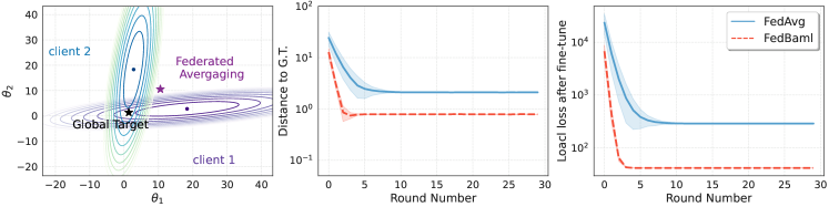
Figure 2: An illustration of federated least squares regression with two clients. Left: Contour plots of each of the quadratic objectives and the corresponding exact global posterior mean (global target). Middle: Convergence curves for our method and FedAvg with 10 steps per round. Right: The curves of local loss for our method and FedAvg after 10 steps of local fine-tuning per round.

5.1 Toy Experiment

To illustrate our method, we start with a simple toy example on a synthetic dataset. We consider a federated regression problem, where the two clients with quadratic objectives of the form:

$$f_{i}(\bm{\theta}) =\log\exp\big{\{}\frac{1}{2}\big{\|}\mathbf{y}_{i}-\mathbf{X}_{i}\bm{\mathrm{w}}\big{\|}^{2}\big{\}}$$

$$=\log\exp\big{\{}\frac{1}{2}(\bm{\mathrm{w}}-\bm{\mu}_{i})^{\top}\bm{\Sigma}_{i}^{-1}(\bm{\mathrm{w}}-\bm{\mu}_{i})\big{\}}+\text{const},$$

where $\mathbf{X}_{i}\in\mathbb{R}^{n_{i}\times d}$ and $\mathbf{y}_{i}\in\mathbb{R}^{n_{i}}$ are synthetic samples from client $i$, $i=1,2$. Here the goal is to infer the mean of the global posterior $p(\bm{\mathrm{w}}|\mathcal{D}_{1},\mathcal{D}_{2})$ from two clients. Assuming an improper uniform prior, each local posterior follows a Gaussian distribution $p_{i}(\bm{\mathrm{w}})\sim\mathcal{N}(\bm{\mu}_{i},\bm{\Sigma}_{i})$, as does the global posterior. Each client approximates its own local posterior, and the server aggregates the obtained results to infer the global posterior. We measure the Euclidean Distance between the mean of approximate posterior $\bm{\mu}_{i}$ and the global target $\bm{\mu}$ (exact global posterior) at each round.

Fig. 2 presents the plotted convergence trajectories of FedABML and FedAvg, where experimental results demonstrate that our method exhibits faster convergence and approaches the global target more closely compared to FedAvg. Given our focus on personalization, it is crucial to assess the extent of per-client improvement achieved through global posterior inference. Therefore, we employ the approximate global posterior as local initialization and investigate the speed of personalization through local fine-tuning. Fig. 2 shows that our method achieves a lower local loss after local fine-tuning. This indicates that our method enables accurate and rapid personalization. The shaded areas in the graph indicate the 95% confidence interval, while the mean and standard deviation metrics are calculated as the average of 5 runs with different initializations and random seeds.

5.2 Experimental Setup

Next, we explore the applicability of our method to nonlinear models and real datasets. Following the same setup in Collins et al. (2021), our method is compared with several competitive baselines on realistic tasks. First of all, we provide a comprehensive overview of our experimental setup.

Datasets and Models.

We conducted experiments on four image datasets:

• FashionMNIST (Xiao et al., 2017): a dataset consisting of images of digits, with a training set containing 60,000 examples and a test set containing 10,000 examples.

• EMNIST (Cohen et al., 2017): a dataset of handwritten characters featuring 62 distinct classes (including 52 alphabetical classes and 10 digital classes). In this paper, we utilize only 10% of the original dataset due to its unnecessarily large number (814,255) of examples for the 2-layer MLP model.

• CIFAR-10 and CIFAR-100 (Krizhevsky et al., 2009): image classification datasets that contain 60,000 colored images with a resolution of $32\times 32$ pixels. Both datasets share the same set of 60,000 input images. However, CIFAR-100 has a finer labeling scheme with 100 unique labels, whereas CIFAR-10 has only 10 unique labels.

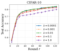
(a) Impact of $\lambda$

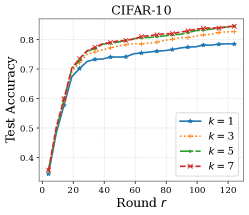
(b) Impact of $k$

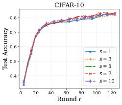
(c) Impact of $s$

Figure 3: Results on CIFAR-10 under various hyperparameters are shown. Observe that our method is robust to changes in the number of Monte Carlo samples $s$, but performs poorly with a larger KL term of $\lambda$ and a smaller number of inner updates $k$.

EMNIST and FashionMNIST are randomly partitioned into $N=150$ and $200$ clients respectively. The CIFAR datasets are also randomly divided among $N=100$ clients. To ensure the heterogeneity in these data, we follow the same procedure used in McMahan et al. (2017), where they partitioned the datasets based on labels and assigned each client at most $S$ classes. Generally, each client is assigned an equal number of training samples and classes, except for the EMNIST dataset. In our experiments, we employ a 5-layer CNN for CIFAR-10, ResNet-18 for CIFAR-100, and 2-layer MLP for EMNIST, as done in (Collins et al., 2021). For FashionMNIST, we apply a multi-class logistic regression.

Table 2: Performance according to the fine-tune epochs on new clients.

	Algorithm	Fine-tune epochs
		0	1	2	3	4	5	8	10
CIFAR-10 (100,2)	FedAvg	$\bm{19.18}$	75.19	75.71	76.42	76.98	77.37	78.11	78.45
	FedProx	19.00	74.77	75.25	75.94	76.52	76.94	77.67	78.01
	Per-FedAvg	18.00	71.29	72.13	73.89	75.22	76.24	78.61	80.08
	pFedMe	14.42	71.99	71.81	71.54	71.68	72.14	72.14	72.33
	pFedbayes	16.95	67.25	67.60	68.46	68.93	68.53	69.40	69.09
	Ours	16.09	$\bm{77.12}$	$\bm{79.61}$	$\bm{80.65}$	$\bm{81.64}$	$\bm{81.75}$	$\bm{83.05}$	$\bm{83.23}$
CIFAR-10 (100,5)	FedAvg	25.54	60.01	60.41	60.65	60.87	60.48	61.51	61.63
	FedProx	24.28	59.04	59.32	59.53	59.73	59.50	60.62	60.52
	Per-FedAvg	19.82	48.08	51.49	52.69	54.05	54.90	57.81	58.71
	pFedMe	20.90	54.81	55.04	55.33	55.46	54.86	55.31	55.48
	pFedbayes	16.99	45.71	48.28	47.99	48.48	47.96	48.77	48.58
	Ours	$\bm{29.52}$	$\bm{62.02}$	$\bm{62.79}$	$\bm{63.76}$	$\bm{64.12}$	$\bm{64.50}$	$\bm{65.40}$	$\bm{66.11}$

Baselines.

We conduct a comprehensive comparison, evaluating our approach against a range of personalized FL approaches, as well as methods that focus on learning a single global model and their fine-tuned counterparts. Among the global FL methods, we consider FedAvg (McMahan et al., 2017), FedProx (Li et al., 2018) and SCAFFOLD (Karimireddy et al., 2020). Among the personalized FL methods, Per-FedAvg (Fallah et al., 2020) and pFedMe (T Dinh et al., 2020) are two meta-learning based approaches that prioritize reference initialization. Additionally, Ditto (Li et al., 2021) simultaneously trains local personalized models and a global model, incorporating extra local updates based on regularization to the global model. pFedbayes (Zhang et al., 2022) can be regarded as a Bayesian extension of FedProx. In addition to these methods, we also include other common personalized FL methods such as FedRep (Collins et al., 2021), FedBABU (Oh et al., 2021), and FedPop (Kotelevskii et al., 2022). Among the above methods, Per-FedAvg, pFedMe, and pFedbayes are most similar to our proposed method. To obtain fine-tuning results, we follow a two-step process. First, we train the global model for the entire training period. Then, each client performs fine-tuning on its local training data, making adjustments to the global model. Finally, we evaluate the test accuracy based on these fine-tuned models.

Implementation.

In each experiment, we sample a fraction of clients at a ratio of $\tau=10\%$ in every communication round. The models are initialized randomly and the training is conducted for a total of $T=100$ communication rounds across all datasets. For all methods, we perform $R=5$ local epochs in all cases. To calculate accuracies, we take the average local accuracies for all clients over the final 10 rounds, except for the fine-tuning methods. The entire training and evaluation process is repeated five times to ensure the robustness of the results.

Hyperparameters.

As in (McMahan et al., 2017), the local sample batch size was set to 50 for each dataset. For each dataset, the learning rates were tuned via grid search in $\{10^{-3},10^{-2},10^{-1.5},10^{-1},10^{-0.5}\}$. The best selected learning rate was $10^{-3}$ for CIFAR datasets and $10^{-2}$ for MNIST datasets. For algorithm-specific hyperparameters, we followed the recommendations provided in their respective papers. For FedProx, we tuned the regularization term $\mu$ among the values $\{0.05,0.1,0.25,0.5\}$ and selected $\mu=0.25$ for CIFAR datasets and $\mu=0.5$ for MNIST datasets. For Ditto, we tuned the $\lambda$ among the values $\{0.25,0.5,0.75,1\}$, and chose $\lambda=0.75$ for all cases. For Per-FedAvg, we used an inner learning rate of $10^{-4}$ and employed the Hessian-free version. The inner learning rate and regularization weight of pFedMe were set to the global learning rate and $\lambda=15$ with $k=5$. For SCAFFOLD, the learning rate on the server was set to $1$ for all cases. For pFedbayes, we tuned $\lambda$ among the values $\{0.05,0.1,0.25,0.5\}$ and used $\lambda=0.05$ with $k=5$.

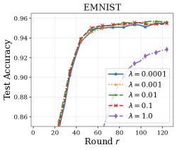
(a) Impact of $\lambda$

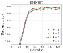
(b) Impact of $k$

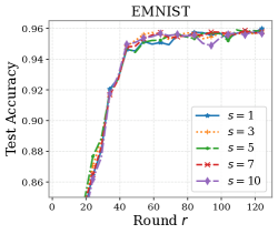
(c) Impact of $s$

Figure 4: Results on EMNIST under various hyperparameters are shown. We observe that the impact of different hyperparameters on convergence is not readily apparent, possibly due to the task’s relative simplicity.

5.3 Performance Comparison

Performance with compared benchmarks.

We present the average local test errors of various algorithms for different settings in Table 1. Our method consistently outperforms or closely matches the top-performing method across all settings. Our proposed algorithms demonstrate superior performance in terms of both accuracy and convergence. Particularly, the performance improvement on the CIFAR-100 dataset is more pronounced than others. This can be attributed to the more efficient optimization capabilities of our method, which are particularly effective on complex datasets.

Generalization to new clients (Fine-tuning performance).

As discussed in Section 4, our method enables easy learning of own personalized models for new clients joining after the distributed training. In the next experiments, we provide an empirical example to evaluate the generalization strength in terms of adaptation for new clients. To do this, we first train our method and several personalized FL methods in a common setting on CIFAR-10, with only 20% of the clients participating to the training. In the second phase, the remaining 80% of clients join and utilize their local training datasets to learn a personalized model. By controlling the number of fine-tuning epochs during the evaluation process, we investigate the speed of personalization for these methods.

Table 2 presents the initial and personalized accuracies of those methods on new clients. Notably, our method achieves higher accuracy with a small number of Fine-tuning epochs, indicating accurate and rapid personalization, especially when fine-tuning is either costly or restricted. The results demonstrate the superior performance of our method compared to the baseline methods.

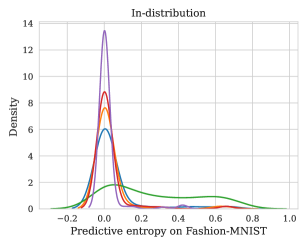
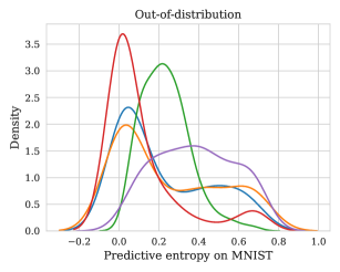
Figure 5: Left: In-distribution with FashionMNIST training. Right: Out-of-distribution with MNIST inference – one curve corresponds to one client. Observe that the client with in-distribution data participating in the training and the client with out-of-distribution data present significantly different patterns.

Uncertainty Quantification.

As mentioned before, a notable advantage of our proposed method over other personalized FL approaches is the ability to quantify uncertainty through local sampling from the posterior distribution. To achieve this, we conducted an out-of-distribution analysis on pairs of training client data and test client data from MNIST/FashionMNIST and CIFAR-10/SVHN. Specifically, we compare the density of predicted entropy for in-distribution (ID) on training clients and out-of-distribution (OOD) data on test clients. it is important to note that the training client and the test client have exactly the same labels. This serves as a measure of uncertainty, given by $\operatorname{Ent}(\mathrm{x})=\sum_{y\in\mathcal{Y}}p(y|\mathrm{x})\log p(y|\mathrm{x})$. These uncertainties can provide insights into how well the model captures the diverse patterns of heterogeneous clients. Based on these insights, we can classify clients and retrain them accordingly.

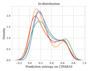
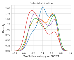
Figure 6: Left: In-distribution with CIFAR-10 training. Right: Out-of-distribution with SVHN inference – one curve corresponds to one client.

In Fig. 5, we present the results of the uncertainty analysis for the MNIST/FashionMNIST pair. In the left part of the figure, we see the distribution of entropy assigned to the in-distribution objects (validation split, but from the same domain as the training data). In the right part, we see the distribution for out-of-distribution data (FashionMNIST in our case). It can be observed that our proposed approach provides relevant uncertainty diagnosis, as indicated by the distinct distributions of entropy for the in-distribution and out-of-distribution data. However, the level of uncertainty captured by Fig. 6, which illustrates the uncertainty distribution for the CIFAR-10/SVHN pair, is not as pronounced as in the MNIST/FashionMNIST example. This could be attributed to the more complex nature of the datasets, which makes it harder to visualize uncertainty.

Impact of other hyperparameters.

Here, we investigate the impact of various parameters on the convergence of our method. We conduct experiments on the EMNIST and CIFAR-10 datasets to analyze the effects of different parameters, including the number of gradient updates $k$, the weight of the $\mathrm{KL}$ term $\lambda$, and the number of Monte Carlo samples $s$. In particular, $k$ allows for approximately finding the personalized model. Figs. 3(b) and 4(b) show that larger values of $k$ (e.g., 7) do not result in significant improvement in convergence. Therefore, we determine that a value of $k=5$ is sufficient for our method. Next, Figs. 3(a) and 4(a) demonstrate the convergence behavior of our method with different values of $\lambda$. We observe that increasing $\lambda$ does not necessarily lead to a substantial improvement in accuracy. Thus, it is crucial to carefully tune the value of $\lambda$ depending on the dataset. Furthermore, the number of Monte Carlo samples considered in practice is often limited. In Figs. 3(c) and 4(c), we observe that larger values of $s$ do not yield significant improvements, and a value of $s=5$ already provides a considerable level of performance.

6 Conclusion

In this paper, we aim to study personalized FL through Amortized Bayesian Meta-Learning and propose a novel approach called FedABML from a probabilistic inference perspective. Moreover, our approach utilizes hierarchical variational inference across clients, enabling the learning of a shared prior distribution. This shared prior plays a crucial role in identifying common patterns among a group of clients and facilitates their individual learning tasks by generating client-specific approximate posterior distributions through a few iterations. In addition, our theoretical analysis provides an upper bound on the average generalization error across all clients, providing insight into the model’s generalization performance and reliability. Furthermore, extensive empirical results validate its effectiveness in rapidly adapting a model to a client’s local data distribution through the use of shared priors. These findings underscore the practical applicability of our approach in real-world federated learning scenarios. Although the probabilistic perspective offers valuable insights for inference and prediction, it comes with the drawback of increased communication overhead due to transmitting variational parameters. To address this limitation, future research could investigate the integration of our approach with compression methods, such as quantization techniques, to effectively reduce the amount of communication required. This would enable more efficient implementation of our approach in large-scale federated learning scenarios.

References

- Al-Shedivat et al. (2020) Maruan Al-Shedivat, Jennifer Gillenwater, Eric Xing, and Afshin Rostamizadeh. Federated learning via posterior averaging: A new perspective and practical algorithms. arXiv preprint arXiv:2010.05273, 2020.
- Bai et al. (2020) Jincheng Bai, Qifan Song, and Guang Cheng. Efficient variational inference for sparse deep learning with theoretical guarantee. Advances in Neural Information Processing Systems, 33:466–476, 2020.
- Bernardo and Smith (2009) José M Bernardo and Adrian FM Smith. Bayesian theory, volume 405. John Wiley & Sons, 2009.
- Blundell et al. (2015) Charles Blundell, Julien Cornebise, Koray Kavukcuoglu, and Daan Wierstra. Weight uncertainty in neural network. In International conference on machine learning, pages 1613–1622. PMLR, 2015.
- Boucheron et al. (2013) Stéphane Boucheron, Gábor Lugosi, and Pascal Massart. Concentration inequalities: A nonasymptotic theory of independence. Oxford university press, 2013.
- Briggs et al. (2020) Christopher Briggs, Zhong Fan, and Peter Andras. Federated learning with hierarchical clustering of local updates to improve training on non-iid data. In 2020 International Joint Conference on Neural Networks (IJCNN), pages 1–9. IEEE, 2020.
- Cao et al. (2023) Longbing Cao, Hui Chen, Xuhui Fan, Joao Gama, Yew-Soon Ong, and Vipin Kumar. Bayesian federated learning: A survey. arXiv preprint arXiv:2304.13267, 2023.
- Chen et al. (2018) Fei Chen, Mi Luo, Zhenhua Dong, Zhenguo Li, and Xiuqiang He. Federated meta-learning with fast convergence and efficient communication. arXiv preprint arXiv:1802.07876, 2018.
- Chen and Chao (2020) Hong-You Chen and Wei-Lun Chao. Fedbe: Making bayesian model ensemble applicable to federated learning. arXiv preprint arXiv:2009.01974, 2020.
- Chen and Chen (2022) Lisha Chen and Tianyi Chen. Is bayesian model-agnostic meta learning better than model-agnostic meta learning, provably? In International Conference on Artificial Intelligence and Statistics, pages 1733–1774. PMLR, 2022.
- Chen et al. (2020) Yiqiang Chen, Xin Qin, Jindong Wang, Chaohui Yu, and Wen Gao. Fedhealth: A federated transfer learning framework for wearable healthcare. IEEE Intelligent Systems, 35(4):83–93, 2020.
- Chérief-Abdellatif (2020) Badr-Eddine Chérief-Abdellatif. Convergence rates of variational inference in sparse deep learning. In International Conference on Machine Learning, pages 1831–1842. PMLR, 2020.
- Cohen et al. (2017) Gregory Cohen, Saeed Afshar, Jonathan Tapson, and Andre Van Schaik. Emnist: Extending mnist to handwritten letters. In 2017 international joint conference on neural networks (IJCNN), pages 2921–2926. IEEE, 2017.
- Collins et al. (2021) Liam Collins, Hamed Hassani, Aryan Mokhtari, and Sanjay Shakkottai. Exploiting shared representations for personalized federated learning. In International Conference on Machine Learning, pages 2089–2099. PMLR, 2021.
- Deng et al. (2020) Yuyang Deng, Mohammad Mahdi Kamani, and Mehrdad Mahdavi. Adaptive personalized federated learning. arXiv preprint arXiv:2003.13461, 2020.
- Dinh et al. (2021) Canh T Dinh, Tung T Vu, Nguyen H Tran, Minh N Dao, and Hongyu Zhang. Fedu: A unified framework for federated multi-task learning with laplacian regularization. arXiv preprint arXiv:2102.07148, 400, 2021.
- Fallah et al. (2020) Alireza Fallah, Aryan Mokhtari, and Asuman Ozdaglar. Personalized federated learning with theoretical guarantees: A model-agnostic meta-learning approach. Advances in Neural Information Processing Systems, 33:3557–3568, 2020.
- Finn et al. (2017) Chelsea Finn, Pieter Abbeel, and Sergey Levine. Model-agnostic meta-learning for fast adaptation of deep networks. In International conference on machine learning, pages 1126–1135. PMLR, 2017.
- Ganguly et al. (2022) Ankush Ganguly, Sanjana Jain, and Ukrit Watchareeruetai. Amortized variational inference: Towards the mathematical foundation and review. arXiv preprint arXiv:2209.10888, 2022.
- Gao et al. (2022) Dashan Gao, Xin Yao, and Qiang Yang. A survey on heterogeneous federated learning. arXiv preprint arXiv:2210.04505, 2022.
- Garnett (2023) Roman Garnett. Bayesian optimization. Cambridge University Press, 2023.
- Grant et al. (2018) Erin Grant, Chelsea Finn, Sergey Levine, Trevor Darrell, and Thomas Griffiths. Recasting gradient-based meta-learning as hierarchical bayes. arXiv preprint arXiv:1801.08930, 2018.
- Guo et al. (2023) Han Guo, Philip Greengard, Hongyi Wang, Andrew Gelman, Yoon Kim, and Eric P Xing. Federated learning as variational inference: A scalable expectation propagation approach. arXiv preprint arXiv:2302.04228, 2023.
- Jiang et al. (2019) Yihan Jiang, Jakub Konečnỳ, Keith Rush, and Sreeram Kannan. Improving federated learning personalization via model agnostic meta learning. arXiv preprint arXiv:1909.12488, 2019.
- Karimireddy et al. (2020) Sai Praneeth Karimireddy, Satyen Kale, Mehryar Mohri, Sashank Reddi, Sebastian Stich, and Ananda Theertha Suresh. Scaffold: Stochastic controlled averaging for federated learning. In International Conference on Machine Learning, pages 5132–5143. PMLR, 2020.
- Kingma et al. (2015) Durk P Kingma, Tim Salimans, and Max Welling. Variational dropout and the local reparameterization trick. Advances in neural information processing systems, 28, 2015.
- Kotelevskii et al. (2022) Nikita Kotelevskii, Maxime Vono, Eric Moulines, and Alain Durmus. Fedpop: A bayesian approach for personalised federated learning. arXiv preprint arXiv:2206.03611, 2022.
- Krizhevsky et al. (2009) Alex Krizhevsky, Geoffrey Hinton, et al. Learning multiple layers of features from tiny images. 2009.
- Kulkarni et al. (2020) Viraj Kulkarni, Milind Kulkarni, and Aniruddha Pant. Survey of personalization techniques for federated learning. In 2020 Fourth World Conference on Smart Trends in Systems, Security and Sustainability (WorldS4), pages 794–797. IEEE, 2020.
- Li et al. (2018) Tian Li, Anit Kumar Sahu, Manzil Zaheer, Maziar Sanjabi, Ameet Talwalkar, and Virginia Smith. Federated optimization in heterogeneous networks. arXiv preprint arXiv:1812.06127, 2018.
- Li et al. (2021) Tian Li, Shengyuan Hu, Ahmad Beirami, and Virginia Smith. Ditto: Fair and robust federated learning through personalization. In International Conference on Machine Learning, pages 6357–6368. PMLR, 2021.
- Liu et al. (2021) Liangxi Liu, Feng Zheng, Hong Chen, Guo-Jun Qi, Heng Huang, and Ling Shao. A bayesian federated learning framework with online laplace approximation. arXiv preprint arXiv:2102.01936, 2021.
- MacKay (1992) David JC MacKay. A practical bayesian framework for backpropagation networks. Neural computation, 4(3):448–472, 1992.
- Mansour et al. (2020) Yishay Mansour, Mehryar Mohri, Jae Ro, and Ananda Theertha Suresh. Three approaches for personalization with applications to federated learning. arXiv preprint arXiv:2002.10619, 2020.
- Marfoq et al. (2021) Othmane Marfoq, Giovanni Neglia, Aurélien Bellet, Laetitia Kameni, and Richard Vidal. Federated multi-task learning under a mixture of distributions. Advances in Neural Information Processing Systems, 34:15434–15447, 2021.
- McMahan et al. (2017) Brendan McMahan, Eider Moore, Daniel Ramage, Seth Hampson, and Blaise Aguera y Arcas. Communication-efficient learning of deep networks from decentralized data. In Artificial intelligence and statistics, pages 1273–1282. PMLR, 2017.
- Neal (2012) Radford M Neal. Bayesian learning for neural networks, volume 118. Springer Science & Business Media, 2012.
- Oh et al. (2021) Jaehoon Oh, Sangmook Kim, and Se-Young Yun. Fedbabu: Towards enhanced representation for federated image classification. arXiv preprint arXiv:2106.06042, 2021.
- Pati et al. (2018) Debdeep Pati, Anirban Bhattacharya, and Yun Yang. On statistical optimality of variational bayes. In International Conference on Artificial Intelligence and Statistics, pages 1579–1588. PMLR, 2018.
- Polson and Ročková (2018) Nicholas G Polson and Veronika Ročková. Posterior concentration for sparse deep learning. Advances in Neural Information Processing Systems, 31, 2018.
- Qu et al. (2022) Zhe Qu, Xingyu Li, Rui Duan, Yao Liu, Bo Tang, and Zhuo Lu. Generalized federated learning via sharpness aware minimization. In International Conference on Machine Learning, pages 18250–18280. PMLR, 2022.
- Ravi and Beatson (2019) Sachin Ravi and Alex Beatson. Amortized bayesian meta-learning. In International Conference on Learning Representations, 2019.
- Razavi-Far et al. (2022) Roozbeh Razavi-Far, Boyu Wang, Matthew E Taylor, and Qiang Yang. An introduction to federated and transfer learning. In Federated and Transfer Learning, pages 1–6. Springer, 2022.
- Reddi et al. (2020) Sashank Reddi, Zachary Charles, Manzil Zaheer, Zachary Garrett, Keith Rush, Jakub Konečnỳ, Sanjiv Kumar, and H Brendan McMahan. Adaptive federated optimization. arXiv preprint arXiv:2003.00295, 2020.
- Smith et al. (2017) Virginia Smith, Chao-Kai Chiang, Maziar Sanjabi, and Ameet S Talwalkar. Federated multi-task learning. Advances in neural information processing systems, 30, 2017.
- T Dinh et al. (2020) Canh T Dinh, Nguyen Tran, and Josh Nguyen. Personalized federated learning with moreau envelopes. Advances in Neural Information Processing Systems, 33:21394–21405, 2020.
- Tan et al. (2022) Alysa Ziying Tan, Han Yu, Lizhen Cui, and Qiang Yang. Towards personalized federated learning. IEEE Transactions on Neural Networks and Learning Systems, 2022.
- Wang et al. (2020) Jianyu Wang, Qinghua Liu, Hao Liang, Gauri Joshi, and H Vincent Poor. Tackling the objective inconsistency problem in heterogeneous federated optimization. Advances in neural information processing systems, 33:7611–7623, 2020.
- Wilson and Izmailov (2020) Andrew G Wilson and Pavel Izmailov. Bayesian deep learning and a probabilistic perspective of generalization. Advances in neural information processing systems, 33:4697–4708, 2020.
- Xiao et al. (2017) Han Xiao, Kashif Rasul, and Roland Vollgraf. Fashion-mnist: a novel image dataset for benchmarking machine learning algorithms. arXiv preprint arXiv:1708.07747, 2017.
- Yang et al. (2020) Hongwei Yang, Hui He, Weizhe Zhang, and Xiaochun Cao. Fedsteg: A federated transfer learning framework for secure image steganalysis. IEEE Transactions on Network Science and Engineering, 8(2):1084–1094, 2020.
- Yoon et al. (2018) Jaesik Yoon, Taesup Kim, Ousmane Dia, Sungwoong Kim, Yoshua Bengio, and Sungjin Ahn. Bayesian model-agnostic meta-learning. Advances in neural information processing systems, 31, 2018.
- Zhang et al. (2023a) Xiaojin Zhang, Yan Kang, Lixin Fan, Kai Chen, and Qiang Yang. A meta-learning framework for tuning parameters of protection mechanisms in trustworthy federated learning. arXiv preprint arXiv:2305.18400, 2023a.
- Zhang et al. (2022) Xu Zhang, Yinchuan Li, Wenpeng Li, Kaiyang Guo, and Yunfeng Shao. Personalized federated learning via variational bayesian inference. In International Conference on Machine Learning, pages 26293–26310. PMLR, 2022.
- Zhang et al. (2023b) Xu Zhang, Wenpeng Li, Yunfeng Shao, and Yinchuan Li. Federated learning via variational bayesian inference: Personalization, sparsity and clustering. arXiv preprint arXiv:2303.04345, 2023b.
- Zhao et al. (2018) Yue Zhao, Meng Li, Liangzhen Lai, Naveen Suda, Damon Civin, and Vikas Chandra. Federated learning with non-iid data. arXiv preprint arXiv:1806.00582, 2018.