Evaluating AI systems under uncertain ground truth: a case study in dermatology

Abstract

For safety, AI systems in health undergo thorough evaluations before deployment, validating their predictions against a so-called ground truth. Importantly, this ground truth is assumed known and fixed, i.e., certain. However, especially in health settings, this is actually not the case and the ground truth may be uncertain. Unfortunately, this is largely ignored in standard evaluation of AI models but can have severe consequences such as overestimating the future performance (Gordon et al., 2021). To avoid this, we measure the effects of ground truth uncertainty, which we assume decomposes into two main components: annotation uncertainty which stems from the lack of reliable annotations, and inherent uncertainty due to limited observational information. This ground truth uncertainty is ignored when estimating the ground truth by deterministically aggregating annotations, e.g., by majority voting or averaging. In contrast, we propose a framework where aggregation is done using a statistical model. Specifically, we frame aggregation of annotations as posterior inference of so-called plausibilities, representing distributions over classes in a classification setting, subject to a hyper-parameter encoding annotator reliability. Based on this model, we propose a metric for measuring annotation uncertainty and provide uncertainty-adjusted metrics for performance evaluation. We present a case study applying our framework to skin condition classification from images (Liu et al., 2020) where annotations are provided in the form of differential diagnoses, modeled as partial ranking of conditions. The deterministic adjudication process called inverse rank normalization (IRN) from previous work ignores ground truth uncertainty in evaluation. Instead, we present two alternative statistical models: a probabilistic version of IRN and a Plackett–Luce-based model (Plackett, 1975; Luce, 2012). We find that a large portion of the dataset exhibits significant ground truth uncertainty and standard IRN-based evaluation severely over-estimates performance without providing uncertainty estimates. In contrast, our framework provides uncertainty estimates on common metrics of interest such as top-$k$ accuracy and average overlap, showing that performance can change multiple percentage points depending on the annotator reliability which directly impacts model selection.

1 Introduction

Prior to usage, predictive AI models in health are usually evaluated by comparing model predictions on a held-out test set annotated with a corresponding known ground truth. In a supervised classification context, this typically assumes the availability of a single, unique and certain ground truth per example. In almost all benchmarks for supervised learning, this ground truth is derived by deterministic aggregation of multiple human annotations, e.g., using simple majority voting or averaging, often ignoring any uncertainty or disagreement. For example, in medical diagnosis, doctors hired for labeling examples have to make complex decisions with very limited information. Where doctors would usually ask patients questions or perform additional tests, they instead have to come up with a working hypothesis of possible conditions, a so-called differential diagnosis. On ambiguous cases, doctors with different levels of experience in medicine, different expertise and biases, constrained by an imperfect labeling tool, will come to different conclusions (Freeman et al., 2021).

Instead of ignoring this disagreement and pretending the ground truth to be fixed and certain, we argue that it is important to acknowledge and address this disagreement. This is to ensure the best possible outcome for the patient because disagreement often reflects individual challenges that when ignored pose significant risks. Specifically, we state that ground truth is uncertain. This uncertainty can be decomposed into annotation uncertainty and inherent uncertainty. The former stems from an imperfect labeling process: even expert annotators can make mistakes; tasks might be subjective, annotators might be biased, inexperienced in using the labeling tool or simply lack experience in the labeling task. The inherent uncertainty, on the other hand, stems from limited observational information. In the example above, there might be ambiguous cases where inferring a clear condition for a patient solely on a single image or a short report, can be extremely difficult. This also includes what related work calls task ambiguity (Uma et al., 2022) (e.g., if classes are not agreed upon (Phene et al., 2019; Medeiros et al., 2023)). In practice, ground truth uncertainty is manifested through disagreement among annotators (e.g., measured by inter-annotator disagreement) and it is challenging to attribute disagreement to annotation or inherent uncertainty (Abercrombie et al., 2023; Röttger et al., 2022). However, while recruiting a larger group of annotators, training them better or improving the labeling tool can reduce annotation uncertainty (usually at a very high cost), inherent uncertainty is generally irresolvable (Schaekermann et al., 2016). This also holds for adjudication (Schaekermann et al., 2019b; Duggan et al., 2021). Moreover, deterministically aggregating more annotators may eliminate minority views (Field et al., 2021).

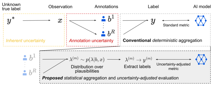
Figure 1: Ground truth uncertainty in supervised AI systems such as classification: The unobserved ground truth $y^{*}$ is assumed to yield an observation $x$. This observation can contain limited information giving rise to inherent uncertainty where the true label might not be clearly identifiable purely from $x$. Nevertheless, experts are asked to provide annotations $b^{1},\dots,b^{R}$ based on $x$. These are subject to annotation uncertainty caused by the lack of reliable annotations. See Figure 5 for a concrete example in skin condition classification. These annotations are then typically (deterministically) aggregated and a single estimate $y$ of the true label $y^{*}$ is extracted. Evaluation of AI models uses the estimate $y$ as ground truth, ignoring any ground truth uncertainty. In contrast, we use statistical aggregation to explicitly model distributions over ground truth labels, so-called plausibilities $\lambda$, representing categorical distributions over classes. The distribution over $\lambda$ captures annotation uncertainty; the plausibilities themselves may capture inherent uncertainty. We discuss how to measure annotation uncertainty and evaluate AI systems on top of these plausibilities.

We can observe annotator disagreement in many standard datasets (see Figure 3 for an example on CIFAR10 (Krizhevsky, 2009; Peterson et al., 2019)). For many of these benchmarks, ground truth uncertainty is limited to a small fraction of examples while the ground truth of the majority of examples can be trusted. In medicine, in contrast, it is common that a significant portion of examples is subject to ground truth uncertainty, observed by high annotator disagreement (Schaekermann et al., 2016). For example, this has recently been shown in skin condition classification (Jain et al., 2021; Eng et al., 2019), but also holds beyond health, e.g., in toxicity classification (see Figure 9). As a result, the problem of ground truth uncertainty has been recognized in several previous works; see e.g. (Sculley, 2007; Cabitza et al., 2020; Northcutt et al., 2021; Uma et al., 2021; Gordon et al., 2021; Davani et al., 2022; Plank, 2022; Leonardelli et al., 2023). Often, however, the focus is on mitigating the symptoms of ground truth uncertainty rather than tackling it directly. For example, there is a large body of work on dealing with label noise (Northcutt et al., 2021). In contrast, we believe that many instances of label errors stem from ignoring the underlying disagreement. In cases where ground truth uncertainty is modeled explicitly, related work focuses on training (Welinder et al., 2010; Rodrigues and Pereira, 2018; Guan et al., 2018) but still assumes certain ground truth for evaluation. This is despite Maier-Hein et al. (2018) explicitly highlighting the impact of ignoring annotator disagreement in evaluation on model selection and ranking. As illustrated in (Gordon et al., 2021), ignoring disagreement by deterministically aggregating annotations may lead to misleading and fragile results when assessing the future performance of AI systems.

We propose here a general framework for measuring and evaluating with ground truth uncertainty based on statistical aggregation of annotations. Essentially, we pose aggregation as a posterior inference task following Figure 1: given multiple annotations and a prior knowledge of annotator reliability, we infer so-called plausibilities. In a classification setting, these plausibilities represent categorical distributions over classes. The variation in plausibilities captures annotation uncertainty. The plausibilities themselves capture inherent uncertainty depending on the entropy of the corresponding categorical distributions. Reliability can be thought of as a model parameter that provides a prior over the expected variation in plausibilities (cf. Figure 2). It could be informed by domain experts or tuned on data (similar to work in crowd sourcing (Yan et al., 2014; Zheng et al., 2017)). However, as quantifying annotator reliability is difficult, we assume it to be a free parameter during evaluation. Then, we propose a measure of annotation certainty to quantify the uncertainty of any label being the true ground truth. This allows us to quantify annotation uncertainty on individual examples as well as on whole datasets. In addition, we present uncertainty-adjusted variants of common classification metrics such as top-k accuracy or average overlap. Altogether, we provide a comprehensive strategy to evaluate AI systems for health under ground truth uncertainty.

In this paper, we apply our framework to skin condition classification from images in dermatology following the setting of (Liu et al., 2020). Here, annotations are expressed as differential diagnoses, i.e., partial rankings. Because classifying skin conditions purely from images is an incredibly difficult task, there is significant disagreement among annotations for a large portion of the dataset. Following (Liu et al., 2020), we consider inverse rank normalization (IRN) as baseline deterministic aggregation method. IRN can be thought of as providing a plausibility point estimate and prior work typically used the top-1 label as ground truth for evaluation – ignoring both annotation and inherent uncertainty. Instead, we propose two alternative statistical models: a probabilistic interpretation of IRN and a Plackett–Luce-based model (Plackett, 1975; Luce, 2012) specifically adapted to partial rankings. Our experiments highlight the high annotation uncertainty in this setting. Moreover, they show that previous IRN-based evaluation significantly over-estimates classifier performance and disregards large variations in performance due to ground truth uncertainty, hindering model selection. We discussed these results with dermatologists and highlight medical implications such as the inability to clearly categorize cases by risk.

2 Framework for evaluation under uncertain ground truth

This section introduces our framework for evaluation of AI systems with ground truth uncertainty. While this paper focuses on a case study in dermatology, we present our framework in general terms and discuss technical details of applying it to the differential diagnosis annotations from (Liu et al., 2020) in Appendix B. We start by introducing notation and give an intuition of our approach on a toy example as well as a standard image recognition task, namely CIFAR10 (Krizhevsky, 2009). We then formalize this intuition by presenting the statistical model we use for modeling how annotator opinions are aggregated. Based on this model, we present measures for annotation uncertainty as well as uncertainty adjusted performance metrics for evaluating AI models.

2.1 Notation and introductory examples

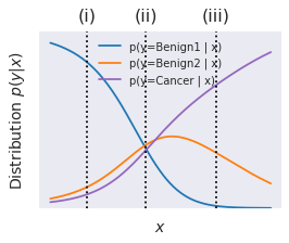
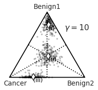
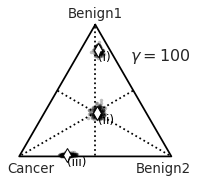
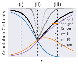
Figure 2: Illustration of annotation certainty on a toy dataset. Left: Synthetic dataset showing one-dimensional observations $x$ and corresponding true distribution $p(y|x)$ over labels $y$ for three imaginary labels Benign1, Benign2 and Cancer. Example (ii) is particularly ambiguous in the sense that $p(y|x)$ is not crisp. Middle left: For illustration, we plot the distribution $p(y|x)$ on the 3-simplex. Middle and middle right: Modeling aggregation of annotator opinions $b$ statistically, see text, allows us to sample plausibilities $\lambda^{(m)}\sim p(\lambda|b,x)$. The spread of these plausibilities around the actual true distributions $p(y|x)$ captures the annotation uncertainty. This is influenced by the annotations as well as a prior reliability parameter $\gamma$. This parameter reflects our a prior trust in the annotators. Right: Measuring how often the top-1 label changes given plausibility samples $\lambda^{(m)}$, we can compute annotation certainty for all examples. We plot annotation certainty across different reliabilities $\gamma$ (black to gray) indicating the effect of different prior trust levels.

For illustration and introducing notation, we consider the synthetic toy dataset of Figure 2 (left). Here, observations $x$ are illustrated as one-dimensional on the x-axis and we plot the true distribution $p(y|x)$ for three different classes (blue, orange and violet) on the y-axis. We highlight three examples, (i), (ii) and (iii), where the latter two are inherently ambiguous, i.e., the corresponding distribution $p(y|x)$ is not crisp. This is intuitively visualized when plotting the distributions $p(y|x)$ on a 3-simplex where the corners would correspond to crisp distributions (middle left). Of course, we never observe the true $p(y|x)$ for these points. Instead, we assume access to a finite set of expert annotations $b$. For simplicity, in this example we assume these annotations to be single labels (sampled from the true $p(y|x)$). Then, we aggregate these opinions to obtain an approximation $\hat{\lambda}$ of $p(y|x)$ and select a label to use as ground truth based on, e.g., majority voting. This represents how labels for many common benchmarks such as CIFAR, ImageNet (Russakovsky et al., 2015) or Hateful Memes (Kiela et al., 2020) have been obtained. We refer to $\hat{\lambda}$ as plausibilities as they construct a distribution $p(y|\hat{\lambda})$ over labels from which the $\arg\max$ corresponds to the majority voted label. However, this approach ignores any uncertainty present in the annotations $b$.

Instead, we assume a distribution $p(\lambda|b,x)$ over plausibilities. Here, we use a Dirichlet distribution with concentration parameters reflecting the annotator opinions as well as a prior reliability parameter ($\gamma$ in Figure 2; also see Appendix A for details). This reliability parameter will quantify our a priori trust in the annotators. For example, we expect reliability to increase with the number of annotators or their expertise and training. However, choosing or estimating reliability can be challenging or require additional information. Instead, we take the reliability to be a free parameter, allowing us different views on the data. This is illustrated in Figure 2 (middle and middle right), showing plausibilities $\lambda^{(m)}\sim p(\lambda|b,x)$, $m\in[M]$, sampled from the statistical aggregation model on the 3-simplex. The spread in these plausibilities represents annotation uncertainty and can be reduced using a higher reliability. The position on the simplex represents inherent uncertainty which is lower for plausibilities close to the corners such as (i) and higher for plausibilities close to the center such as (ii). Then, we compute the top-1 label for every sampled $\lambda^{(m)}$, i.e., the label with the largest plausibility $\arg\max_{k\in[K]}\lambda^{(m)}_{k}$. This allows us to measure annotation certainty (defined formally in Section 2.3) – if the top-1 label is always the same label, there is no annotation uncertainty. Specifically we can measure the fraction of plausibilities $\lambda^{(m)}$ among all $M$ samples where the top-1 label is $k$. Taking the maximum over all labels $k$ defines annotation certainty. In Figure 2 (middle) we plot this annotation certainty for different reliabilities (black and gray) and we clearly see that annotation certainty is consistently low for example (ii), while for (iii) annotation certainty increases with higher reliability. This also allows us to easily summarize annotation uncertainty across the whole dataset.

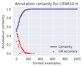
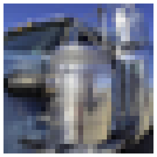
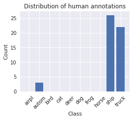
Figure 3: We plot annotation certainty and uncertainty-adjusted (UA) accuracy for CIFAR10-H (Krizhevsky, 2009; Peterson et al., 2019), highlighting the 1000 examples with lowest annotation certainty. There is a small set of $178$ images with certainty below $99\%$ for which annotators tend to disagree. Given the large number of annotators ($50$), this likely indicates examples with inherent uncertainty, as shown for two examples on the right (images and histogram of annotations).

To move from this toy example to a real benchmark, we consider CIFAR10 (Krizhevsky, 2009) with the human annotations from (Peterson et al., 2019). As above, each annotator provides a single label such that we can apply the same methodology. Figure 3 (left) reports the corresponding annotation certainty alongside an uncertainty-adjusted version of accuracy. As can be seen, annotators agree for the majority of examples, resulting in certainties close to $1$. Nevertheless, on roughly $178$ test examples, certainty is below $0.99$. As there are 50 annotators per example with only 10 classes, it is likely that these are actually difficult cases, i.e. cases with inherent uncertainty, as confirmed in Figure 3. This corresponds to roughly $0.2\%$ of the examples. Interestingly, recent improvements in accuracy on CIFAR10 are often smaller than $0.2\%$. To measure accuracy while taking annotation uncertainty into account, we measure how often the original CIFAR10 ground truth labels coincide with the top-1 labels obtained from sampled plausibilities. We call this uncertainty-adjusted accuracy (formally defined in Section 2.4) and, unsurprisingly, observe that the original labels of (Krizhevsky, 2009) (when interpreted as predictions) often perform poorly for examples with high annotation uncertainty (red in Figure 3). We expect the impact of ground truth uncertainty to be significantly more pronounced in settings with more disagreement, especially in our dermatology case study (Liu et al., 2020), but also in other domains. For example, Appendix A includes an example on Wikipedia Toxicity (Wulczyn et al., 2017) and we refer to (Leonardelli et al., 2021) for more examples in NLP.

2.2 Statistical model

The statistical model $p(\lambda|b,x)$ informally introduced above and summarized in Figure 4 is at the core of our framework. Essentially, we propose to replace deterministic aggregation of annotator opinions with a statistical model. To this end, we view aggregation as computing the posterior distribution $p(\lambda|b,x)$ over plausibilities, given annotations $b$ and observations $x$. In all the examples discussed within this paper, we make the simplifying assumption $p(\lambda|b,x)=p(\lambda|b)$ such that plausibilities are inferred solely from the annotator opinions. Then, plausibilities represent distributions over labels:

$$p(y|b,x)=\int p(y|\lambda)p(\lambda|b,x)\mathrm{d}\lambda.$$ (1)

We compute this posterior by specifying the annotation process, i.e., $p(b|\lambda)$ and assuming a prior $p(\lambda)$ independent of the input $x$. The annotation process specifies how we expect experts to provide their annotations if we knew the underlying distribution $\lambda$ over labels. Additionally, we assume a reliability parameter as part of our statistical model. In practice, this often corresponds to a temperature parameter in $p(b|\lambda)$ (e.g., $\gamma$ in our toy example from Figure 2). However, we interpret it as quantifying the prior trust we put in the annotators. As fixing this parameter based on domain expertise or data is challenging, we treat it as a free parameter that is to be explored during evaluation.

On CIFAR10, we assumed each annotator to provide the top-1 label. Thus, it was simple to derive the posterior in closed form for a Dirichlet prior distribution. Here, the plausibilities $\lambda$ explicitly correspond to the categorical distribution over classes $p(y|x)$. In other cases, where annotations do not directly match the label space (see Appendix A for examples), this statistical model might be more complex. For our case study, a skin-condition classification problem detailed in Section 3, the expert annotations are partial rankings instead of top-1 labels. In this case, the plausibilities $\lambda$ approximate the categorical distribution $p(y|x)$ as for CIFAR10 but we will rely on a Plackett–Luce model for $p(b|\lambda)$ (Plackett, 1975; Luce, 2012). Unfortunately, this means that the posterior $p(\lambda|b)$ is not available in closed-form so specific techniques are needed to sample from it; see Appendix B.

Figure 4: Graphical model corresponding to the statistical aggregation model at the core of our framework: This describes the joint distribution of the observation $x$, plausibilities $\lambda$, annotations $b=(b^{1},...,b^{R})$ and label $y$. We observe $x$ and $b$ from which one can infer plausibilities $p(\lambda|b,x)$ and label $p(y|\lambda)$, see text. As discussed in the text, in order to simplify inference of $\lambda$, we assume a simplified model with $p(\lambda|b,x)=p(\lambda|b)$.

Our model in Figure 4 comes with assumptions and limitations that are important to highlight. First, we assume the annotators to be conditionally independent given the plausibilities. This is a simplification and there is significant work in crowd sourcing and truth discovery considering alternative models (Yan et al., 2014). Second, as discussed previously, in all our examples, we consider a simplified version of the model in Figure 4, assuming conditional independence $p(\lambda|b,x)=p(\lambda|b)$. This makes inferring the posterior over $\lambda$ easier but clearly reduces our ability to model input dependent uncertainty and thereby disentangle the different sources of uncertainty outlined above. This means that $p(\lambda|b)$ can only capture the uncertainty present in the annotations. This reduces our ability to decide whether the uncertainty stems mainly from limited observational information or from the annotation process. For example, it is difficult to distinguish between an inherently ambiguous example where we observed low disagreement by chance and an actually unambiguous example with low disagreement. However, this distinction would be extremely valuable, e.g., to inform relabeling. Finally, it is important to realize that this introduces a model assumption in our certainty and performance metrics. For example, there is no guarantee that $p(y|b,x)$ converges to the true $p(y|x)$ as the number of annotators goes to infinity as the annotation model can be mis-specified. However, all existing benchmarks are based on an assumed annotation model. That this assumption is implicit and often unacknowledged does not change the fact that it has tangible effects on evaluation.

2.3 Annotation certainty

To formalize our measure for annotation uncertainty as described above, we consider a fixed but arbitrary label $y\in[K]$. This could be a deterministically aggregated ground truth as on CIFAR10 or, in Section 2.4, a prediction from a classifier. Then, we informally define the certainty for a specific label $y$ as the probability that $y$ corresponds to the top-1 label of the plausibilities $\lambda$, given the input $x$ and annotations $b$ as well as the chosen statistical model. More formally, we can write this as an expectation over $p(\lambda|b,x)$:

$$\text{Certainty}(y;b,x)=p(y=\arg\max_{j}\lambda_{j})=\mathbb{E}_{p(\lambda|b,x)}\Big{\{}\delta\left[{y=\arg\max_{j}\lambda_{j}}\right]\Big{\}}.$$ (2)

where $\delta[\cdot]\in\{0,1\}$ is the indicator function for an event. In practice, we compute it using a Monte Carlo average

$$\text{Certainty}(y;b,x)\approx\frac{1}{M}\sum_{m=1}^{M}\delta\left[{y=\arg\max_{j}\lambda_{j}^{(m)}}\right],\quad\text{where\leavevmode\nobreak\ }\lambda^{(m)}\overset{\textup{i.i.d.}}{\sim}p(\lambda|b,x).$$ (3)

This estimates certainty for a specified label $y$. To summarize annotation certainty for an example, we compute the maximum certainty across all possible labels $y$:

$$\text{AnnotationCertainty}_{1}(b,x)=\max_{y\in[K]}\text{Certainty}(y;b,x).$$ (4)

Here, the subscript $1$ indicates that annotation certainty refers to the top-1 label from plausibilities. However, we can similarly generalize this to sets of labels $C$, e.g., top-$j$ sets with $|C|=j$:

$$\text{AnnotationCertainty}_{j}(b,x)=\max_{C:\text{ top-}j\text{ labels}}\text{Certainty}(C;b,x)$$ (5)

with $$\text{Certainty}(C;b,x)=\mathbb{E}_{p(\lambda|b,x)}\Big{\{}\delta\left[{C=Y_{\text{top}-|C|}(\lambda)}\right]\Big{\}}.$$ (6)

This certainty measure can also be estimated using $M$ Monte Carlo samples. This prevents us from having to enumerate all $K!/(j!(K-j)!)$ subsets of size $j$ as seemingly implied by (5), which would be prohibitive. Instead, we only need to consider top-$j$ sets corresponding to the $M$ samples. However, larger $j$ might require a higher $M$ for reliable estimates of annotation certainty. To measure annotation certainty of a dataset, we can average AnnotationCertainty($b,x$) across examples.

There are some caveats of our measure of annotation certainty to be aware of, most of them depending on the aggregation procedure $p(\lambda|b,x)$. For example, Equation (5) is always $1$ for any input where the model $p(\lambda|b,x)$ is a point mass; i.e., it gives a single deterministic point estimate $\hat{\lambda}$ (subject to there being ties, which we ignore for simplicity). This is, by construction the case in any deterministic aggregation procedure for human annotations. Also, with an infinite number of annotators $p(\lambda|b,x)$ will typically converge to a point mass $\hat{\lambda}$ such that annotation certainties converge to $1$. However, this does not mean that the plausibilities correspond to an unambiguous one-hot distribution over classes. Finally, annotation certainties for the same problem depend on the used statistical aggregation process and the reliability we attribute to annotators. This also means that annotation certainty is not a metric that is to be minimized. This is trivially possible, for example, by putting infinite trust in annotators and working with a point estimate $\hat{\lambda}$ (infinite reliability $\gamma$ in Figure 2).

Considering the 3-simplex in Figure 2, annotation certainty measures the impact of the spread in plausibilities on the top-$j$ labels. Thereby, annotation certainty implicitly also captures inherent uncertainty: even a small spread in plausibilities changes the top-$j$ labels more often for inherently uncertain examples, i.e., plausibilities close to the center of the simplex. More generally, this means that annotation certainty will be high for easy, unambiguous examples that all annotators agree on. The reverse, however, is not necessarily true: low annotation certainty can indicate high inherent uncertainty but it does not necessarily have to. For example, many experienced annotators consistently disagreeing might indicate high inherent uncertainty; however, annotators might also disagree for other reasons such as unclear annotation instructions, even if the example is generally easy to classify. This also explains our naming: annotation certainty explicitly measures annotation uncertainty and only implicitly accounts for inherent uncertainty. Partly, this also stems from our assumption that $p(\lambda|b,x)=p(\lambda|b)$ in Section 2.2, making it more difficult to disentangle annotation and inherent uncertainty.

2.4 Uncertainty-adjusted accuracy

Given a measure of annotation certainty, we intend to take it into account when evaluating performance of AI models. Specifically, we assume the label set $C$ used in Equation (5) to be a prediction set from a classifier – for example, corresponding to the top-$k$ logits of a deep neural networks. Then, we wish to measure the quality of this prediction set. If we knew the true plausibilities $\lambda^{*}=p(y|x)$, our ground truth target $Y_{\text{top}-j}(\lambda^{*})$ would be chosen as the top-$j$ elements of $\lambda^{*}$. The quality of the prediction can then be computed by evaluating the indicator of the event that the target set is contained within the prediction set, $\delta\left[{Y_{\text{top}-j}(\lambda^{*})\subseteq C_{\text{top}-k}(x)}\right]\in\{0,1\}$, assuming $j\leq k$ for simplicity). For example, the standard top-$k$ accuracy is an estimate of the probability where we specifically take $j=1$ and define

$$\text{Accuracy}_{\text{top}-k}=p(Y_{\text{top}-1}(\lambda^{*})\subseteq C_{\text{top}-k}(x))=\mathbb{E}_{p(x)}\{\delta\left[{Y_{\text{top}-1}(\lambda^{*})\subseteq C_{\text{top}-k}(x)}\right]\}.$$ (7)

However, we acknowledge that we cannot know $\lambda^{*}$ and that there is uncertainty on $\lambda$. Luckily, given $p(\lambda|b,x)$, we can quantify this uncertainty using Certainty from Equation (3). Integrating this into the above definition of accuracy yields the proposed uncertainty-adjusted version:

$$\text{UA-Accuracy}_{\text{top}-k}=p(Y_{\text{top-}1}(\lambda)\subseteq C_{\text{top-}k}(x))=\mathbb{E}_{p(x)}\mathbb{E}_{p(\lambda|b,x)}\{\delta[Y_{\text{top-}1}(\lambda)\subseteq C_{\text{top-}k}(x)]\}.$$ (8)

Note that this metric now implicitly depends on the annotations $b$ through our statistical model $p(\lambda|b,x)$. As with annotation certainty, this metric mainly accounts for annotation uncertainty and is only indirectly aware of inherent uncertainty (see Section 2.3). In order to explicitly account for inherent uncertainty, i.e., the plausibilities $\lambda$ not having a clear top-$1$ label, we can compare the top-$j$ target set $Y_{\text{top-}j}(\lambda)$ with the top-$k$ prediction set $C_{\text{top-}k}(x)$ set. However, to avoid extensive notation, we consider only target sets having the same cardinality as the prediction set. We call this metric uncertainty-adjusted top-$k$ set accuracy:

$$\text{UA-SetAccuracy}=p(Y_{\text{top}-|C|}(\lambda)=C(x))=\mathbb{E}_{p(x)}\mathbb{E}_{p(\lambda|b,x)}\{\delta\left[{Y_{\text{top}-|C|}(\lambda)=C(x)}\right]\}.$$ (9)

This deviates slightly from the notion of standard top-$k$ (vs. top-$1$) accuracy, but can be more appropriate when evaluating under uncertain ground truth where a large part of the uncertainty stems from inherent uncertainty. In such cases, the top-$1$ label will often be a poor approximation of the ground truth. In practice, we approximate these uncertainty-adjusted metrics using a Monte Carlo estimate.

Uncertainty-adjusted accuracy reduces to standard accuracy as soon as there is no annotation uncertainty or it is ignored through deterministic aggregation (i.e., when a point estimate $\hat{\lambda}$ is used). As with annotation certainty, uncertainty-adjusted metrics primarily capture annotation uncertainty and do not necessarily capture inherent uncertainty if it is not reflected in the annotations. This is particularly important to highlight for uncertainty-adjusted top-$k$ accuracy, which only considers the top-1 label from sampled plausibilities $\lambda^{(m)}$. For very ambiguous examples, this can ignore inherent uncertainty if the annotation uncertainty is low such that most plausibilities $\lambda^{(m)}$ agree on the top-1 label. To some extent this is mitigated by using our uncertainty-adjusted set accuracy. However, as our approach of constructing uncertainty-adjusted metrics is very general, this can also be addressed by considering different “base” metrics.

For example, we illustrate the applicability of our framework on a class of ranking metrics: Specifically, for large prediction set sizes $k=|C|$, the annotation certainty can be very low as achieving exact match of large prediction and target sets can be a rare event. Thus, it seems natural to consider less stringent metrics based on the intersection of prediction set $C$ and ground truth set $Y$ instead of requiring equality:

$$\text{Overlap}(C,Y)=\frac{|C\cap Y|}{|C|}.$$ (10)

As we do not know the target ground truth set, we use instead the expectation under the aggregation procedure $p(\lambda|b,x)$ where we define an uncertainty adjusted overlap as

$$\text{UA-Overlap}(C,x)=\mathbb{E}_{p(\lambda|b,x)}\Big{\{}\text{Overlap}(C,Y_{\text{top}-|C|}(\lambda))\Big{\}}.$$ (11)

Now, following (Wu and Crestani, 2003; Webber et al., 2010), we consider overlaps of increasingly larger prediction and ground truth sets and define uncertainty adjusted average overlap as

$$\text{UA-AverageOverlap@L}=\mathbb{E}_{p(x)}\Big{\{}\frac{1}{L}\sum_{k=1}^{L}\text{UA-Overlap}(C_{\text{top-}k}(x),x)\Big{\}}.$$ (12)

Similar uncertainty-adjusted variants can be defined for other ranking-based metrics (Sakai, 2013), e.g., Kendall’s tau or Spearman’s footrule (Shieh, 1998; Fagin et al., 2003, 2004; Kumar and Vassilvitskii, 2010; Vigna, 2015). In general, we expect that uncertainty-adjusted variants can easily be defined for almost all relevant metrics in machine learning.

3 Case study: skin condition classification

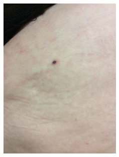
A0: {Pyogenic granuloma} {Hemangioma} {Melanoma}
A1: {Angiokeratoma of skin} {Atypical Nevus}
A2: {Hemangioma} {Melanocytic Nevus, Melanoma, O/E - ecchymoses present}
A3: {Hemangioma, Melanoma, Skin Tag}
A4: {Melanoma}
A5: {Hemangioma} {Melanoma} {Melanocytic Nevus}

Image and annotations

 

Plausibilities

 

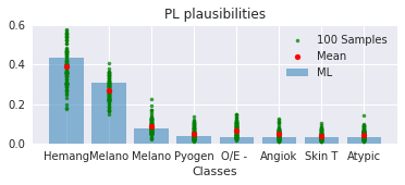
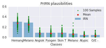
Pred.

Model A: $C_{\text{top-}3}=$
{Atyp. Nevus, Hemangioma, Melanocytic Nevus}

Model B: $C_{\text{top-}3}=$
{Hemangioma, Melanocytic Nevus, Melanoma}

 

Eval.

Model A	PL	PrIRN
$\mathbb{E}_{p(\lambda|b,x)}\{\delta[Y_{\text{top-}1}(\lambda)\subseteq C_{\text{top-}3}(x)]\}$	$0.7$	$0.52$

Model B	PL	PrIRN
$\mathbb{E}_{p(\lambda|b,x)}\{\delta[Y_{\text{top-}1}(\lambda)\subseteq C_{\text{top-}3}(x)]\}$	$1$	$0.99$

Figure 5: An example from our case study: Given images (one shown), the task is to predict a set out of $419$ different skin conditions. For evaluation, six annotators provided (partial) rankings of potential ground truth conditions (top row). Given these annotations, our statistical aggregation models, PL and PrIRN, produce distributions over plausibilities (samples indicated in green), contrasted with deterministic aggregation such as IRN or ML (blue). These plausibilities represent categorical distributions over all conditions (second row). We then evaluate uncertainty-adjusted metrics based on these plausibilities: given prediction sets for models A and B (third row), we evaluate how often, in expectation, the top-1 label from the plausibilities is included (bottom row).

We demonstrate our framework on a case study in dermatology: skin condition classification from images (Liu et al., 2020). Here, several dermatologists provide annotations in the form of differential diagnoses, i.e., partial rankings of classes (see Figure 5). Based on previous work (Eng et al., 2019; Jain et al., 2021), we expect significant disagreement among annotators indicating a high degree of uncertainty in the ground truth. Following (Liu et al., 2020), we initially use inverse rank normalization (IRN) for deterministic aggregation. We then introduce two statistical aggregation models: a probabilistic version of IRN (PrIRN) as well as a Plackett–Luce (Plackett, 1975; Luce, 2012) (PL) based model. Both models include a reliability parameter described in Section 2 that reflects our trust in the annotators. Selecting a range of reliabilities, we evaluate annotation certainty as well as uncertainty-adjusted accuracy of classifiers in a range of different trust scenarios. Across reliabilities, we observe very high annotation uncertainty in the dataset of (Liu et al., 2020) and discuss implications for evaluating and selecting classifiers.

3.1 Dataset and methods

The dataset of (Liu et al., 2020) includes $K=419$ different conditions which are to be predicted from three $448\times 448$ pixel images taken with consumer-grade cameras. This is illustrated in Figure 5 (top row), showing one of the input images alongside the corresponding annotations from six dermatologists. Each annotation includes a variable number of conditions combined with a confidence value. As these confidence values are not comparable across dermatologists, previous work (Eng et al., 2019; Roy et al., 2022; Azizi et al., 2022) uses them to obtain (partial) rankings of conditions (made explicit by braces in Figure 5). Details and statistics on the annotations are provided in Appendix C. Following (Liu et al., 2020), we use inverse rank normalization (IRN) to obtain a point estimate of plausibilities. Specifically, IRN weights each condition by its inverse rank, i.e., $\nicefrac{{1}}{{j}}$ for the $j$-th condition, sums across annotations and re-normalizes. We use these plausibilities to train several classifiers using the cross-entropy loss by varying architecture and hyper-parameters following (Roy et al., 2022). We randomly selected four of these classifiers for evaluation and comparison. In prior work, evaluation is based purely on the top-1 IRN label (i.e., the classifier is evaluated against the argmax of IRN plausibilities), ignoring both evidence of lower ranked conditions as well as the uncertainty induced through the aggregated annotations.

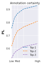
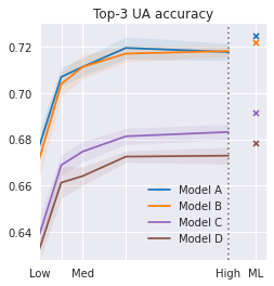
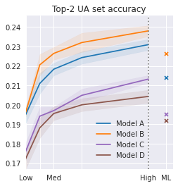
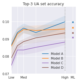
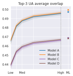
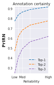
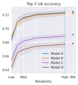
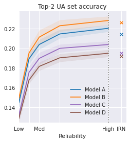
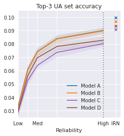
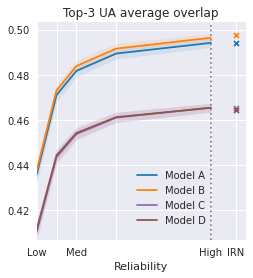
Figure 6: For PL (top) and PrIRN (bottom), we plot annotation certainty as well as uncertainty-adjusted top-3 accuracy, top-2 and top-3 set accuracy and top-3 average overlap (y-axis). We consider four classifiers, A to D, across various reliabilities (x-axis). We omit exact reliability values as they are inherently not comparable between PL and PrIRN. Annotation certainty and evaluation metrics are averages across all examples and $M=1000$ plausibility samples. The shaded region additionally reports the standard deviation of metrics after averaging across plausibility samples; colored $\times$ mark performance against point estimates (ML for PL, IRN for PrIRN). We find that reliability severely impacts evaluated performance and that there is a significant variation induced by annotation uncertainty. Moreover, classifiers tend to perform significantly worse when evaluated against more than the top-1 labels using set accuracy.

In contrast, we propose two alternative statistical aggregation models following Section 2: a probabilistic version of IRN (PrIRN), and a Plackett–Luce (PL) based model. PrIRN interprets the IRN plausibilities $\hat{\lambda}$ as a maximum likelihood estimate of the parameters of a multinomial distribution. The posterior $p(\lambda|b)$ for sampling plausibilities is accordingly defined to be a Dirichlet distribution $\mathcal{D}(\gamma\hat{\lambda})$ where $\gamma$ is the aforementioned reliability parameter. Instead, PL is a standard model for rankings of conditions that we extend to handle partial rankings. PL assumes a categorical distribution over conditions from which annotators sample without replacement. Assuming independent gamma priors on plausibilities, a Gibbs sampler allows to efficiently sample plausibilities from the corresponding posterior. Similar to IRN, we consider the maximum likelihood (ML) estimate under PL likelihood as a deterministic counterpart to modeling the full posterior. Like PrIRN, PL model can also accommodate a reliability parameter that specifies our trust into the annotators. In both models, higher reliability will result in higher annotation certainty, cf. Equation (2). As it is generally unclear what the “right” reliability should be, we perform experiments across a range of reliabilities, corresponding to different scenarios of how much we trust our annotators. We refer to Appendix B for an in-depth description of both approaches, including several technical contributions in applying PL to partial rankings.

Plausibilities from PrIRN and PL for a particular difficult case are shown in Figure 5 (second row). Compared to ML and IRN (blue bars), there is clearly significant variation in the sampled plausibilities (green dots) to the extent that the two most likely conditions (Hemangioma and Melanoma) may swap their positions. This also impacts evaluation: considering the two prediction sets from Figure 5 (third row), the first model (A) does not include both conditions, while the second model (B) does. Concretely, model A includes the top-1 label in only 70% of the sampled plausibilities, while model B always includes the top-1 label (100%), cf. Figure 5 (fourth row). In a nutshell, this summarizes our evaluation methodology on one specific case with fixed reliability, which we extend to the whole test set and across multiple reliabilities next.

3.2 Results

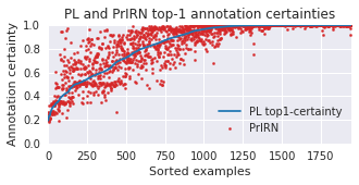
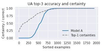
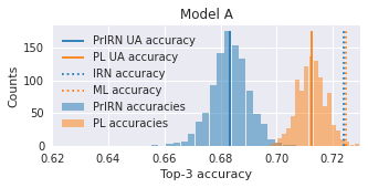
Figure 7: For a fixed, medium reliability, we present annotation certainty and uncertainty-adjusted top-3 accuracy across examples and plausibility samples. Left: PL top-1 annotation certainty plotted against sorted examples (blue) in comparison to PrIRN (red). While there is high correlation between PL and PrIRN, there can be significant difference for individual examples. Middle: Uncertainty-adjusted top-3 accuracy for model A against sorted examples (blue). For many examples, the classifier does not consistently include all possible top-1 ground truth label in its predictions, resulting in values between $0$ and $1$. Right: Histogram plot of uncertainty-adjusted top-3 accuracy (averaged over examples) across the $M=1000$ plausibility samples. Between worst- and best-case plausibilities, there can be up to 4% difference in accuracy.

Our main results focus on evaluating (top-k) annotation certainty (see Equation (5)) alongside uncertainty-adjusted accuracy (see Equation (8)) across classifiers and reliabilities. As reliabilities are inherently not comparable across PL and PrIRN, we omit specific values. Then, Figure 6 (first column) highlights that average annotation certainty clearly increases with higher reliability; eventually being $1$ at infinite reliability. Also, top-$2$ and top-$3$ annotation certainty is significantly lower than top-1 annotation certainty, meaning that there is significant uncertainty not only in the top-1 condition but also lower ranked ones. This annotation uncertainty also has a clear impact on accuracy: Uncertainty-adjusted top-3 accuracy (second column) reduces significantly for lower reliability. As indicated by the shaded region, there is also high variation in accuracy across plausibility samples. In contrast, the ML and IRN plausibility point estimates, as used in previous work (Liu et al., 2020), typically overestimate performance and cannot provide an estimate of the expected variation in performance.

In order to account for inherent uncertainty in the evaluation, i.e., plausibilities not being crisp distributions, we additionally consider set accuracy in Figure 6 (third and fourth columns). Strikingly, set accuracy is dramatically lower than standard accuracy, highlighting that the trained classifiers perform poorly on conditions likely ranked second or third. This is further emphasized by the fact that the reduction in accuracy is significantly larger than the corresponding drop in annotation certainty. Moreover, shifting focus to set accuracy also impacts the ranking of classifiers. This may has severe implications for hyper-parameter optimization and model selection which is typically based purely on standard accuracy. We also observe more significant differences between using PrIRN and PL, e.g., in terms of absolute accuracy numbers, their variation, or differences across classifiers. This highlights the impact that the statistical aggregation model can have on evaluation. As we might not want to put equal weight on all top-3 ground truth labels equally, Figure 6 (last column) also shows top-3 uncertainty-adjusted average overlap, where second and third condition are weighed by $\nicefrac{{1}}{{2}}$ and $\nicefrac{{1}}{{3}}$, respectively. Besides resulting in generally higher numbers, this also reduces variation significantly.

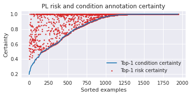
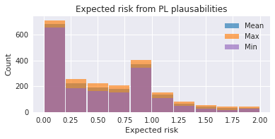
Figure 8: Implications of ground truth uncertainty on risk categories. Right: Annotation certainty computed for risks in red in comparison to conditions blue. Going from 419 conditions to 3 risk levels clearly increases annotation certainty on average. But for many examples, risk categories remain very uncertain. Right: For many examples, there is evidence for multiple risk categories within the annotations. We plot a histogram of expected risk, the expected risk categories given the plausibilities, i.e., distributions over conditions.

In the following, we focus on a fixed, medium reliability (as annotated in Figure 6) and consider annotation certainty and uncertainty-adjusted accuracy across examples. Specifically, Figure 7 (left) plots annotation certainty from PL (blue) and PrIRN (red) over examples (sorted for PL): For at least a quarter of the examples there is significant annotation uncertainty, i.e., top-1 annotation certainty is well below $1$. We also observe that annotation certainty is strongly correlated between PL and PrIRN (correlation coefficient 0.9). This indicates that similar examples are identified as having high annotation uncertainty. However, on individual examples, there can still be a significant difference. Similarly, we found that annotation certainty correlates well with annotator disagreement (see Appendix D). Figure 7 (middle) also shows uncertainty-adjusted top-3 accuracy against (sorted) examples. Again, for at least a quarter of examples, uncertainty-adjusted accuracy lies in between $0$ and $1$, i.e., the top-3 prediction sets do not always include all possible top-1 ground truth labels. In Figure 7 (right), we also show results across plausibility samples might implicate in terms of aggregate statistics. While Figure 6 depicted the variability based on plausibility samples only through standard deviation error bars, these histograms clearly show that accuracy can easily vary by up to 4% between best and worst case.

Besides performance evaluation across all 419 distinct conditions, previous work (Roy et al., 2022) also put significant focus on classifying risk categories, considering low, medium or high risk conditions. These categories are assigned to each condition independent of the actual case (e.g., Melanoma is a high-risk condition). As recommendations to users (e.g., whether the user should see a specialist) are similar for conditions in the same risk categories, it is often more important to correctly classify risk categories compared to individual conditions. Figure 8 (left), however, shows that these risk categories are also subject to significant uncertainty. This is made explicit by computing top-1 annotation certainty for risks categories (red) derived from the plausibilities over conditions. While this is generally higher than annotation certainty for conditions (blue) due to the smaller label space (3 risks vs. 419 conditions), annotation certainty remains low for many cases. This also has far-reaching consequences for evaluation. For example, evaluation metrics such as accuracy are often conditioned on high-risk cases. That is, for evaluation, we are interested in a classifier’s accuracy only considering high-risk cases. This conditioning, however, is not well defined in light of this uncertainty. This is made explicit in Figure 8 (right) which plots expected risk: the expected risk assignment for cases, based on plausibility samples, after mapping risk levels to an ordinal scale; low = 0, medium = 1, and high = 2. Most cases do not yield crisp risk assignments as there is typically evidence for multiple risk categories present in the annotations.

3.3 Discussion

We also qualitatively evaluated our framework in an informal study with two US board-certified dermatologists familiar with the labeling tool (Liu et al., 2020). Specifically, we discussed individual cases with particularly low annotation certainty by showing input images alongside meta information (sex, age, etc.) and the corresponding annotations (cf. Figure 5). Discussing these cases takes considerable time while the dermatologists try to understand how the annotators came to their respective conclusions. In most cases, the disagreement was attributed to inherent uncertainty, i.e., missing information, inconclusive images, etc. In only few cases, the disagreement was attributed to annotator mistakes or annotation quality in general – e.g., inexperienced annotators, annotators ignoring meta information etc. Again, this highlights the difficulty of disentangling annotation and inherent uncertainty in cases with high disagreement (as discussed in Sections 2.2 and 2.3) and is in line with related work on “meta-annotation” for understanding sources of disagreement (Sandri et al., 2023; Bhattacharya et al., 2019). However, this also highlights that our uncertainty-adjusted metrics appropriately take both sources of uncertainty into account.

The results for this case study indicate, using our annotation certainty measure, that a large portion of the dataset exhibits high ground truth uncertainty. The current approach (Liu et al., 2020) of deterministically aggregating annotations using IRN and then evaluating against the corresponding top-1 labels largely ignores this uncertainty. In our framework, using the PrIRN model, this implicitly corresponds to evaluation at infinite reliability, i.e., full trust in all annotators. Instead, our approach to evaluation paints a more complete picture by computing uncertainty-adjusted (top-k) accuracy across a range of reliabilities, corresponding to different trust “scenarios”. In practice, this not only allows to compare models across these different scenarios but also highlights the expected variation in performance. Moreover, we show that performance is always relative to the chosen aggregation model, as highlighted using our alternative Plackett-Luce (PL) (Plackett, 1975; Luce, 2012) based model. As feedback from dermatologists indicates that most of this ground truth uncertainty stems from inherently ambiguous cases, we also explored metrics considering more than the top-1 conditions for evaluation. Here, performance drops rather drastically, indicating potential negative consequences for patients when lower ranked conditions are not appropriate. For example, seemingly random conditions on the 2nd or 3rd place of the prediction set can easily lead to confusion or anxiety. Overall, we believe that our framework will help with model development and make model selection more robust and thereby positively influence patient outcome.

4 Related work

Annotator disagreement has been discussed extensively and early on in medicine (Feinstein and Cicchetti, 1990; McHugh, 2012; Raghu et al., 2019; Schaekermann, 2020) as well as machine learning (Dawid and Skene, 1979; Smyth et al., 1994). Natural language processing, for example, has particularly strong work on dealing with disagreement (Reidsma and op den Akker, 2008; Aroyo and Welty, 2014, 2015; Schaekermann et al., 2016; Dumitrache et al., 2019; Röttger et al., 2022; Abercrombie et al., 2023), see (Pavlick and Kwiatkowski, 2019) for an overview. As crowdsourcing human annotations has become a standard tool in creating benchmarks across the field (Kovashka et al., 2016; Sorokin and Forsyth, 2008; Snow et al., 2008) – though not without criticism (Röttger et al., 2021) – most work focuses on resolving or measuring disagreement and aggregating annotations. Methods for measuring disagreement (Feinstein and Cicchetti, 1990; Powers, 2012; Uma et al., 2021) are often similar across domains. However, measures such as Fleiss’/Cohen’s kappa (Cohen, 1960; Fleiss et al., 2003), percent agreement (McHugh, 2012), or intra-class correlation coefficient (Landis and Koch, 1977) are only applicable to annotations with single class responses such that generalized approaches (Braylan et al., 2022) or custom measures are used for more structured annotations (Pavlick and Kwiatkowski, 2019). Resolving disagreement is typically done computationally (e.g., through majority vote). However, recent work has explored domain-specific interactive approaches for resolving disagreement, involving discussions or deliberation (Schaekermann et al., 2020b, a, 2019a; Schaekermann, 2020; Pradhan et al., 2022; Drapeau et al., 2016; Chen et al., 2019b; Silver et al., 2021; Bakker et al., 2022) or relabeling (Sheng et al., 2008), and reducing disagreement by co-designing labeling with experts (Freeman et al., 2021). Recent work also considers properly modeling disagreement (Vitsakis et al., 2023) or performing meta analysis (Sandri et al., 2023; Bhattacharya et al., 2019), trying to understand sources of disagreement. For benchmarks, disagreement is generally addressed by aggregating labels from multiple annotators to arrive at what is assumed to be the single correct label. This can involve basic majority voting or more advanced methods (Dawid and Skene, 1979; de Marneffe et al., 2012; Pham et al., 2017; Warby et al., 2014; Carvalho and Larson, 2013; Gaunt et al., 2016; Tian et al., 2019), including inverse rank normalization (IRN) as discussed in this paper. Often, aggregation is also performed using probabilistic models from the crowdsourcing and truth-discovery literature (Yin et al., 2008; Welinder and Perona, 2010; Li et al., 2012; Dong et al., 2009; Zhao et al., 2012; Wang et al., 2012; Bachrach et al., 2012; Rodrigues and Pereira, 2018; Guan et al., 2018; Chu et al., 2021; Gordon et al., 2022), see (Yan et al., 2014; Zheng et al., 2017) for surveys. However, evaluation is often based on point estimates and the impact of annotator disagreement on evaluation is generally poorly understood (Gordon et al., 2021). While, e.g., (Reidsma and op den Akker, 2008; Collins et al., 2022) train models on individual annotators, (de Marneffe et al., 2012; Nie et al., 2020) perform evaluation on aggregated probabilities instead of top-1 labels, and (Gao et al., 2017) trains on label distributions rather than discrete aggregated labels, there is no common understanding for dealing with annotation uncertainty for evaluation. Instead, following (Plank, 2022), disagreement is often treated as label noise. Here, early work (Angluin and Laird, 1987; Kearns, 1998; Kearns and Li, 1993; Lawrence and Schölkopf, 2001) assumes uniform or class-conditional label noise, while more recent work (Beigman and Klebanov, 2009; Oyen et al., 2022) also considers feature-dependent or annotator-dependent noise. Popular methods try to estimate the label noise distributions (Northcutt et al., 2019; Hendrycks et al., 2018) in order to prune or re-weight examples. Such approaches have also been utilized to infer annotator confusion matrices (Zhang et al., 2020; Tanno et al., 2019), similar to annotator quality in crowdsourcing. We refer to (Chen et al., 2019a; Zhang et al., 2022) for good overviews and note that there is also some similarity to partial label learning (Hüllermeier and Beringer, 2005; Nguyen and Caruana, 2008; Cour et al., 2011; Wang et al., 2022).

Overall, work on handling annotation disagreement is very fragmented, as highlighted above and in recent surveys (Uma et al., 2021). Moreover, many works treat symptoms such as label noise rather than treating annotator disagreement as uncertainty in the ground truth. This is emphasized in recent position papers (Baan et al., 2022; Plank, 2022; Basile et al., 2021) that argue for common frameworks to deal with this challenge. Indeed, recent work (Sculley, 2007; Maier-Hein et al., 2018; Cabitza et al., 2020; Belz et al., 2023) demonstrates that many results in machine learning are not reproducible, in part due to annotation uncertainty. This has also been the basis for several workshops and challenges on directly learning with disagreement (Leonardelli et al., 2023). Closest to our work, (Gordon et al., 2021; Lovchinsky et al., 2020) propose methods to incorporate label disagreement into evaluation metrics. However, their work is limited to binary classification tasks. Moreover, the considered annotations are unstructured, i.e., annotators merely provide single labels. In contrast, our framework for evaluation with annotation uncertainty if independent of task, domain or annotation format. In contrast to our findings, (Chen et al., 2021) argues that label noise in validation sets can still lead to reliable model selection on rather unambiguous datasets such as CIFAR10. Finally, (Collins et al., 2022) evaluates against labels aggregated from random subsets of annotators on CIFAR10-H, which can be seen as a bootstrapping approach to statistical aggregation in our framework.

5 Conclusion

In this paper, we proposed a framework for evaluating AI models under uncertain ground truth. We believe that ground truth uncertainty stems from annotation uncertainty as well as inherent uncertainty and is typically observed in terms of annotator disagreement: in almost all supervised learning tasks, ground truth labels are implicitly or explicitly obtained by aggregating annotations, e.g., counting frequencies and majority voting. Unfortunately, this type of deterministic aggregation typically ignores the underlying uncertainty which can have severe consequences for safety-critical applications such as health. Instead, we introduce a framework based on a statistical model for aggregating annotations that explicitly accounts for uncertainty. Further, we propose a novel measure of annotation uncertainty and present uncertainty-adjusted metrics for evaluating and comparing AI systems. Applied to a case study in skin condition classification, our framework allowed us to make several important observations that previous work (Liu et al., 2020) missed: First, a large portion of cases exhibits high ground truth uncertainty which, according to dermatologists, often stems from inherent uncertainty. Second, classifier performance often degrades and exhibits significant variation under our uncertainty-adjusted metrics. Third, classifiers perform poorly when taking into account inherent uncertainty by evaluating not only against possible top-1 ground truth labels. Our framework can readily be applied to other settings by adapting the statistical aggregation model to the annotations at hand. We believe that properly accounting for ground truth uncertainty in evaluation will play a critical role in successfully tackling more nuanced and ambiguous tasks.

Data availability

The de-identified dermatology data used in this paper is not publicly available due to restrictions in the data-sharing agreements.

*

Appendix A Further introductory examples and details

Toy dataset and CIFAR10: For our toy dataset as well as CIFAR10, we model $p(\lambda|b,x)=\mathcal{D}(\lambda;\mu)$ as Dirichlet distribution with concentration parameter vector $\mu$. We define $\mu=\gamma s+\alpha\mathbf{1}$ where $s$ is a vector of sufficient statistics with the $c$’th element $s_{c}$ denoting the number of annotators that have chosen $c$ as (top-1) label, $\gamma>0$ is the reliability parameter, $\alpha>0$ is a small prior parameter that we assign to each label $c$, and $\mathbf{1}$ a vector of ones of the same shape as $s$. As shown in Figure 2, a higher reliability parameter $\gamma$ makes the plausibilities $\lambda\sim p(\lambda|b)$ more concentrated, resulting in higher annotation certainty. Here, the effect of $\alpha$ vanishes with higher reliability or more annotators; essentially, $\alpha$ represents a minimum number of annotators.

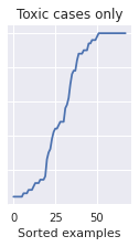
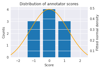
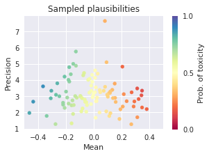
Figure 9: Annotation certainty for 1k examples from the Wikipedia toxicity dataset (Wulczyn et al., 2017) as well as those examples identified by the majority of annotators as toxic or very toxic. On the right, we show an example score distribution and samples from the corresponding posterior over plausibilities. Certainty is low for approximately $50\%$ of the toxic examples.

Wikipedia Toxicity (Wulczyn et al., 2017) is a natural language dataset for detecting toxicity in comments posted in Wikipedia page discussions. Around 10 annotators rate each comment between -2 (very toxic) and 2 (very healthy). Then, a comment can be treated as toxic if the mean rating is below 0. This suggests that the scores are assumed to be normally distributed. In this case, we define the plausibilities as the mean and standard deviation: $\lambda=(\mu,\sigma^{2})$. As before, plausibilities parameterize the distribution over targets. Choosing an appropriate prior for $\mu$ and $\sigma$ allows to calculate certainty as the maximum of the two possible outcomes: $\mathcal{N}(y\leq 0;\mu,\sigma^{2})$ and $\mathcal{N}(y>0;\mu,\sigma^{2})$. Figure 9 shows the computed certainties for the first 1k examples of the dataset. A significant part of the examples is highly uncertain, especially among the toxic cases (majority of annotators responding -2 or -1, roughly 1% of all cases). We also show one qualitative example with the corresponding annotations and plausibility samples. Note that, in this case, plausibilities correspond to one-dimensional Gaussian distributions which are plotted using mean and precision.

AVA (Murray et al., 2012) is a dataset of visual aesthetics scores. Photography enthusiasts and experts rated more than 200k images on a scale between 1 and 10. Compared to CIFAR10, this is a more subjective and thus ambiguous labeling task. Nevertheless, the dataset is commonly used for predicting visual aesthetics, e.g., by predicting poor or good images (Lu et al., 2014; Esfandarani and Milanfar, 2018). For simplicity, this can be done by taking the mean of the ratings and classifying images with mean score lower than $5$ as poor and those with mean score higher or equal to $5$ as good. This suggests that the scores are assumed to be normally distributed. Specifically, $\lambda=(\mu,\sigma^{2})$, modeling mean and standard deviation. Using the same normal-inverse-gamma prior as above, we can compute certainty by estimating $\mathcal{N}(y\leq 5;\mu,\sigma^{2})$ and $\mathcal{N}(y>5;\mu,\sigma^{2})$. Figure 10 shows the computed certainties as well as an example of a typical score distribution and plausibility samples. Surprisingly, for the first 10k images of AVA, most examples receive high certainty. However, this does not imply that there is no inherent ambiguity, as highlighted in Figure 10. Instead, it might just show that there is lower annotation uncertainty due to the high number of, on average, $222$ annotations.

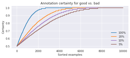
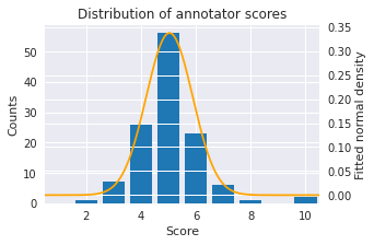
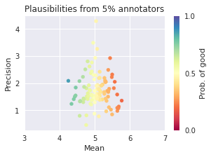
Figure 10: Left: Annotation certainty for the first 10k AVA (Murray et al., 2012) images considering a binary classification setting of poor images (score $<5$) against good images (score $\geq 5$). Certainty might be high primarily due to the large number of annotators. Right: Score distribution for one example together with samples from the corresponding posterior $p(\lambda=(\mu,\sigma^{2})|b)$.

Appendix B Methods for differential diagnoses in health

Having presented our general framework in Section 2, we present in this section technical details and specific methods for applying our methodology to differential diagnosis as observed in our dermatology case study. As indicated in Section 3, we model differential diagnoses as partial rankings and discuss meaningful aggregation models $p(\lambda|b,x)$ that facilitate sampling plausibilities. Specifically, we follow (Liu et al., 2020), and use inverse rank normalization (IRN) as deterministic aggregation as well as propose a probabilistic variant. We also show how a Plackett–Luce model (Plackett, 1975; Luce, 2012) can be adapted to this case. Remember that in this paper we assume $p(\lambda|b,x)=p(\lambda|b)$ in our aggregation schemes.

B.1 Modeling annotations as partial rankings

We model differential diagnoses as partial rankings. In our case study, for each case, each annotator selects a subset of conditions they think might be the true diagnosis. In addition, they assign a confidence score to each condition, indicating how likely they think that condition is the true diagnosis. The subsets of conditions selected by different annotators may differ in size. Moreover, the confidence scores are usually not comparable across annotators which is why they are instead used to produce a ranking of the conditions for each annotator (Liu et al., 2020). This results in partial rankings because there may be ties among conditions (i.e., conditions with the same confidence score) and the large majority of possible conditions remains unranked. Formally, we write

$$b=(b_{{}{}{1}}\succ b_{{}{}{2}}\ldots\succ b_{{}{}{L}}).$$ (13)

We call groups of tied conditions “blocks”, and each block contains one or more labels, $b_{{}{}{i}}=\{{\sigma_{{i}{1}}},\ldots,{\sigma_{{i}{|b_{{}{}{i}}|}}}\}$ with ${\sigma_{{i}{j}}}\in[K]$ and $K$ being the number of classes. Here, $b_{{}{}{i}}\succ b_{{}{}{j}}$ indicates that classes in the $i$-th block are ranked higher than those in the $j$-th block (according to the confidence scores). We assume the blocks are non-empty, mutually exclusive, i.e., $\emptyset\neq b_{{}{}{i}}\subseteq[K]$ and $b_{{}{}{i}}\cap b_{{}{}{j}}=\emptyset$, and that $\bigcup_{i=1}^{L}b_{i}=[K]$. Note that there might exist multiple equivalent permutations within the individual blocks $b_{i}$ such that we use $\mathcal{S}(b)$ to denote the set of all permutations compatible with Equation (13). In the literature discussing ranking metrics and aggregation (Sakai, 2013; Webber et al., 2010; Sculley, 2007; Wu and Crestani, 2003), partial rankings are also commonly referred to as top-$k$ rankings with ties. While some metrics such as Kendall’s tau and Spearman’s footrule have been adapted to ties (Fagin et al., 2004; Vigna, 2015), modeling partial rankings is generally non-trivial. This also holds for any aggregation model $p(\lambda|b,x)$ as we will see in Section B.4.

As an example, we recall annotator 2 from Figure 5 where the blocks are defined as

$$b=(b_{1}=\{\textit{Hemangioma}\},b_{2}=\{\textit{Melanocytic Nevus},\textit{Melanoma},\textit{O/E}\}).$$

We interpret the above example as follows: the annotator declares that Hemangioma is their first choice, followed by either Melanocytic Nevus, Melanoma, or O/E. However, for the latter three conditions, the annotator is unable to say which one is more likely than the others. That is, these three conditions are tied for the second rank. Implicitly, this means that all $3!=6$ possible permutations would be equivalent:

$$(\textit{Hemangioma},\textit{Melanocytic Nevus},\textit{Melanoma},\textit{O/E}),$$

$$(\textit{Hemangioma},\textit{Melanoma},\textit{Melanocytic Nevus},\textit{O/E}),$$

$$\ldots$$

$$(\textit{Hemangioma},\textit{O/E},\textit{Melanocytic Nevus},\textit{Melanoma}).$$

The larger the individual blocks, the larger the number of compatible permutations becomes. Also, annotators usually ignore a large set of conditions. Strictly speaking, the ignored conditions can be thought of as another block, such that

$$b=(b_{1}=\{\textit{Hemangioma}\},b_{2}=\{\textit{Melanocytic Nevus},\textit{Melanoma},\textit{O/E}\},b_{3}=\{\text{\color[rgb]{1,0,0}any other condition}\})$$

with the last block $b_{L}=b_{3}$ capturing all unranked classes. We say that annotators provide a full ranking if all blocks except $b_{L}$ have size one, i.e., $|b_{i}|=1$, $i<L$. We say the annotators provide a complete ranking if all blocks are of size one, i.e., $|b_{i}|=1$, $i\leq L$. Note that we can have multiple annotators providing partial rankings, in which case we let $b^{r}$, $r\in[R]$, denote the annotation by the annotator $r$ out of $R$ annotators.

B.2 Inverse rank normalized (IRN) aggregation

An intuitive method for aggregating differential diagnoses to arrive at a plausibility point estimate is inverse rank normalization (IRN) (Liu et al., 2020). Given a partial ranking $b$ from a single annotator with $L$ blocks as in Equation (13), we define the unnormalized IRN score of a condition $y$ as

$$\text{unnormalizedIRN}(y;b)=\sum_{i=1}^{L-1}\frac{\nicefrac{{1}}{{i}}}{|b_{{}{i}{}}|}\delta[y\in b_{{}{i}{}}].$$ (14)

Unnormalized IRN assigns a weight $\nicefrac{{1}}{{i}}$ to each block $b_{{}{i}{}}$, $i=1,\dots,L-1$ and a weight of $0$ for all the classes in the last block $b_{{}{}{L}}$ of unranked classes. The weight is distributed equally across all classes in a block, i.e., class ${\sigma_{{i}{j}}}$ obtains weight $\nicefrac{{{1/i}}}{{|b_{{}{i}{}}|}}$. Given $R$ partial rankings $b^{1},\ldots,b^{R}$ from $R$ annotators, we define the unnormalized IRN score of a condition $y$ as

$$\text{unnormalizedIRN}(y;b^{1},\ldots,b^{R})=\sum_{r=1}^{R}\text{unnormalizedIRN}(y;b^{r})$$ (15)

with $L_{r}$ being the number of blocks for annotator $r$ and $b_{j}^{r}$ indexing these blocks. Normalized IRN is

$$\text{IRN}(y;b^{1},\ldots,b^{R})=\text{unnormalizedIRN}(k;b^{1},\ldots,b^{R})/\sum_{k=1}^{K}\text{unnormalizedIRN}(k;b^{1},\ldots,b^{R}).$$ (16)

Note that normalization comes after aggregation rather than normalizing per annotator $r$ first and then averaging. Overall, IRN can be viewed as an adhoc point estimate of the plausibilities $\lambda$ without an explicit generative model for $p(\lambda|b,x)$. This also implies that we cannot sample plausibilities from $p(\lambda|b,x)$. In contrast, the next section describes a probabilistic version of IRN that allows to sample plausibilities.

B.3 Probabilistic IRN (PrIRN) aggregation

To derive a probabilistic variant of IRN (PrIRN), we interpret the calculation of unnormalizedIRN as a counting method for accumulating the statistics of a histogram on discrete data. Then, the normalized $\text{IRN}(y;b^{1},\ldots,b^{R})$ corresponds to a maximum likelihood estimate of the parameters of a multinomial distribution (the sampling distribution of a histogram) given the accumulated statistics. In this spirit, we define the sampling distribution $p(\lambda|b^{1},\ldots,b^{R})$ directly as a Dirichlet distribution $\mathcal{D}(\gamma\hat{\lambda})$ where $\hat{\lambda}_{y}=\text{IRN}(y;b^{1},\ldots,b^{R})$ and $\gamma>0$ (the concentration parameter) represents our reliability parameter. Here, the $\mathcal{D}(\gamma\hat{\lambda})$ distribution is the true posterior distribution of the parameters of a categorical distribution if labels were drawn i.i.d. and the observed counts would be $\gamma\hat{\lambda}$. Then, the reliability parameter $\gamma$ can be interpreted as the number of annotators: with increasing number of annotators we have less annotation uncertainty and for $\gamma\rightarrow\infty$ the Dirichlet distribution degenerates to a point mass on $\hat{\lambda}$ – the IRN estimate.

B.4 Plackett–Luce (PL) aggregation

One conceptual problem of PrIRN is that its weighting and aggregation choices seem to be arbitrary, in the sense of not being justified by an explicit generative model for the annotation process, i.e. $p(b|\lambda)$. Another alternative is defining a generative model, and inferring the plausibilities accordingly. More specifically, this would imply defining a likelihood $p(b|\lambda)$, and estimating $\lambda$ accordingly. Having defined a likelihood, one option would be obtaining a maximum likelihood estimate of $\lambda$ under the observations $b$. Another option is to define a prior $p(\lambda)$, and then infer $\lambda$ using the posterior $p(\lambda|b)$.

As we are dealing with rankings, the Plackett–Luce (PL) (Plackett, 1975; Luce, 2012) model is a natural choice for the likelihood $p(b|\lambda)$. It models how annotators, given the true plausibilities $\lambda$, draw full rankings by sampling without replacement from all conditions. Although very appropriate for our problem, unfortunately, the posterior of the plausibilities cannot be derived analytically under the Bayesian variants of this model. However, efficient Gibbs sampling algorithms (Caron and Doucet, 2010; Francois et al., 2012) and optimization procedures (Hunter, 2003) do exist. Here, we extend the Gibbs sampler of (Caron and Doucet, 2010) to partial rankings. Importantly, our sampler will have to be correct and efficient for partial rankings, i.e., with ties and unranked conditions.

In the following, we assume a single case for brevity, with the annotator being indexed by $r\in[R]$ and assume the plausibilities $\lambda_{k}$, $k\in[K]$, to be non-negative. The inferential procedure we describe can be repeated for any other case independently. We also assume that

$$p({\sigma}|\lambda)=\prod_{r=1}^{R}p({\sigma^{{r}}}|\lambda),$$ (17)

meaning that the annotators’ rankings are independent, conditioned on plausibilities. Then, moving to the description of $p({\sigma^{{r}}}|\lambda)$, the classical PL model assumes that each annotator $r$ reports a full ranking of classes by sampling without replacement, proportional to the plausibilities $\lambda$, such that the first class ${\sigma^{{r}}_{{}{1}}}$ is drawn with probability

$$p({\sigma^{{r}}_{{}{1}}}=k)=\frac{\lambda_{k}}{Z}$$

where the normalization constant is $Z=\sum_{k^{\prime}}\lambda_{k^{\prime}}$. Then the annotator draws the next choice ${\sigma^{{r}}_{{}{2}}}$ (by excluding the previous choice ${\sigma^{{r}}_{{}{1}}}$) from $\{1\dots K\}\setminus\{{\sigma^{{r}}_{{}{1}}}\}$ with probability

$$p({\sigma^{{r}}_{{}{2}}}=k|{\sigma^{{r}}_{{}{1}}})=\frac{\lambda_{k}}{Z-\lambda_{{\sigma^{{r}}_{{}{1}}}}}$$

and the next choice ${\sigma^{{r}}_{{}{3}}}$ from $\{1\dots K\}\setminus\{{\sigma^{{r}}_{{}{1}}},{\sigma^{{r}}_{{}{2}}}\}$ with probability

$$p({\sigma^{{r}}_{{}{3}}}=k|{\sigma^{{r}}_{{}{1}}},{\sigma^{{r}}_{{}{2}}})=\frac{\lambda_{k}}{Z-\lambda_{{\sigma^{{r}}_{{}{1}}}}-\lambda_{{\sigma^{{r}}_{{}{2}}}}}$$

and so on until no choices are left. Then, the log-likelihood of the plausibility vector $\lambda$ given the choices ${\sigma^{{r}}}$ is given as

$$\mathcal{L}_{r}(\lambda)=\log\lambda_{{\sigma^{{r}}_{{}{1}}}}-\log Z+\log\lambda_{{\sigma^{{r}}_{{}{2}}}}-\log(Z-\lambda_{{\sigma^{{r}}_{{}{1}}}})+\dots+\log\lambda_{{\sigma^{{r}}_{{}{K}}}}-\log\left(Z-\sum_{k=1}^{K-1}\lambda_{{\sigma^{{r}}_{{}{k}}}}\right).$$

Given Equation (17), the log-likelihood for the entire parameter vector $\lambda$ is simply the equal contributions of all the annotators that have rated the case $\mathcal{L}(\lambda)=\sum_{r}\mathcal{L}_{r}(\lambda)$.

The inferential goal of interest is estimating the latent plausibilities $\lambda$ based on the annotations $b$ in the form of full rankings $\sigma$. As mentioned before, this can be done according to maximum likelihood by maximizing $\mathcal{L}(\lambda)$, or in a Bayesian way by assigning a prior distribution $p(\lambda)$ and inferring the posterior distribution $p(\lambda|{\sigma})\propto p(\lambda)\prod_{r}p({\sigma^{{r}}}|\lambda)$. As the maximum likelihood solution provides a point estimate of the plausibilities, similar to IRN, here we focus on the Bayesian approach.

We can also introduce the equivalent of a reliability parameter $\gamma$ for the PL distribution by defining a new tempered PL distribution with parameters $\bar{\lambda}=\lambda^{\gamma}$ and normalization $\bar{Z}=\sum_{k}\bar{\lambda}_{k}=\sum_{k}\lambda^{\gamma}_{k}$. Unfortunately, the resulting model no longer enjoys the conjugacy properties needed for deriving a Gibbs sampling algorithm. While it is possible to use more generic sampling methods such as Hamiltonian Monte Carlo (HMC) for this tempered PL model, qualitatively we obtain the same concentration effect by simply repeating the partial rankings for each annotator such that the likelihood contribution of each annotator to the posterior is $\gamma\mathcal{L}_{r}(\lambda)$ where $\gamma$ is a small integer. This also matches the intuition of the reliability parameter $\gamma$ in PrIRN from the previous section.

The PL model as introduced above defines a distribution over full rankings. While it is straightforward to compute the probability of a given full ranking under the PL distribution, partial rankings – especially with larger block sizes – provide a computational challenge as we need to consider all the permutations compatible with the partial rankings. This would amount to a computational complexity that scales factorially in the block size. In contrast, the next section describes a procedure for computing the exact likelihood for partial rankings that scales only exponentially in the block sizes.

B.4.1 Exact likelihood computation for partial rankings

For a more concise exposition, we will temporarily assume that we have a single annotator providing a partial ranking $b$, and will introduce the multiple annotator formulation at the end of Section B.4.2. We see that for the partitioning $b=(b_{{}{}{1}},b_{{}{}{2}},\dots,b_{{}{}{L}})$ the probability $p(b|\lambda)=p(b_{{}{}{1}}\succ b_{{}{}{2}}\succ\dots\succ b_{{}{}{L}})$ admits the factorization

$$p(b|\lambda) =p(b_{{}{}{1}}|\lambda)p(b_{{}{}{2}}|\lambda,b_{{}{}{1}})\dots p(b_{{}{}{L-1}}|\lambda,b_{{}{}{1:L-2}}).$$

Note that above we have redefined $b$ to include all unranked classes, if any, in $b_{L}$, such that $b_{1}\cup\dots\cup b_{L}=[K]$, hence we omit the term $p(b_{L}|\lambda,b_{1:L-1})=1$.

Here, the first term is the probability of drawing a permutation from the PL distribution that starts with a sequence of classes that are all in $b_{{}{}{1}}$:

$$p(b_{{}{}{1}}|\lambda)=p(b_{{}{}{1}}\succ(b_{{}{}{2}}\cup b_{{}{}{3}}\cup\dots\cup b_{{}{}{L}}))=\sum_{\sigma}\delta\left[{\sigma_{1:|b_{{}{}{1}}|}\in\mathcal{S}(b_{{}{}{1}})}\right]p(\sigma|\lambda).$$

Remember that $\mathcal{S}(b)$ refers to all permutations compatible with Equation (13). With a slight abuse of notation, we let $\mathcal{S}(b_{{}{}{1}})$ be the set containing all possible permutations of the first block. Concatenating all classes such that $\sigma_{1:|b_{{}{}{i}}|}$ corresponds to the first block, this is essentially the probability that the prefix $\sigma_{1:|b_{{}{}{1}}|}$ is in the first block $b_{{}{}{1}}$. Now, we define the cumulative sum of block sizes as $c_{l}=|b_{1}|+|b_{2}|+\dots+|b_{l}|$ with $c_{0}=0$ and $c_{L}=K$ and get

$$\begin{split}p(b_{{}{}{2}}|\lambda,b_{{}{}{1}})&=p(b_{{}{}{2}}\succ(b_{{}{}{3}}\cup\dots\cup b_{{}{}{L}})|b_{{}{}{1}}\succ(b_{{}{}{2}}\cup b_{{}{}{3}}\cup\dots\cup b_{{}{}{L}}))\\ &=\frac{p(b_{{}{}{1}},b_{{}{}{2}}|\lambda)}{p(b_{{}{}{1}}|\lambda)}=\frac{\sum_{\sigma}\delta\left[{\sigma_{c_{0}+1:c_{1}}\in\mathcal{S}(b_{{}{}{1}})}\right]\delta\left[{\sigma_{c_{1}+1:c_{2}}\in\mathcal{S}(b_{{}{}{2}})}\right]p(\sigma|\lambda)}{\sum_{\sigma}\delta\left[{\sigma_{c_{0}+1:c_{1}}\in\mathcal{S}(b_{{}{}{1}})}\right]p(\sigma|\lambda)}\end{split}$$

for the second block. This suggests that we can generalize this for any arbitrary block $l\in[L]$ as follows:

$$p(b_{{}{}{l}}|\lambda,b_{{}{}{1:l-1}})=\frac{\sum_{\sigma}\Big{(}\prod_{\kappa=1}^{l}\delta\left[{\sigma_{c_{\kappa-1}+1:c_{\kappa}}\in\mathcal{S}(b_{{}{}{\kappa}})}\right]\Big{)}p(\sigma|\lambda)}{\sum_{\sigma}\Big{(}\prod_{\kappa=1}^{l-1}\delta\left[{\sigma_{c_{\kappa-1}+1:c_{\kappa}}\in\mathcal{S}(b_{{}{}{\kappa}})}\right]\Big{)}p(\sigma|\lambda)},$$

with the convention that $b_{{}{}{1:0}}=\emptyset$. This still requires to enumerate all the permutations in $\mathcal{S}(b)$ which is factorial in the length of the blocks. However, the computation can be reduced through an algorithm reminiscent of dynamic programming as one can show that

$$p(b_{{}{}{l}}|\lambda,b_{{}{}{1:l-1}}) =\Big{(}\prod_{k\in b_{{}{}{l}}}\lambda_{k}\Big{)}\cdot\mathcal{R}_{l}({b_{{}{}{l}}}).$$

Here, $\mathcal{R}_{l}(A)$ is a function that is defined recursively for any subset $A\subset b_{{}{}{l}}$ as

$$\mathcal{R}_{l}(A)=\left\{\begin{array}[]{cc}1&A=\emptyset\\ \Big{(}\sum_{a\in A}\mathcal{R}_{l}(A\setminus\{a\})\Big{)}/{\Big{(}\bar{Z}_{l}+\sum_{a\in A}\lambda_{a}\Big{)}}&A\neq\emptyset\end{array}\right.$$

where $\bar{Z}_{l}=\sum_{k\in\bar{b}_{l}}\lambda_{k}$ denotes the total plausibility of the remaining elements $\bar{b}_{l}=b_{{}{}{l+1}}\cup\dots\cup b_{{}{}{L}}$. The probability of a partition is

$$p(b|\lambda) =\Pr\{b_{{}{}{1}}\succ b_{{}{}{2}}\succ\dots\succ b_{{}{}{L}}\}=\Big{(}\prod_{k\notin b_{L}}\lambda_{k}\Big{)}\prod_{l=1}^{L-1}\mathcal{R}_{l}(b_{l}).$$

We refer to Appendix B.4.3 for a proof and an example, but illustrate the recursion in Figure 11.

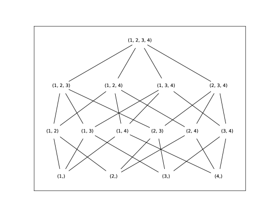
Figure 11: Hasse diagram of subsets of $\{1,2,3,4\}$. To compute the probability of a partial order of the form $\{1,2,3,4\}\succ\bar{b}$ exactly under a PL distribution with parameters $\lambda$, we associate the value $\mathcal{R}(A)$ with each node $A\subset\{1,2,3,4\},A\neq\emptyset$. After initialization of the bottom nodes, that correspond to subsets with only a single element, the algorithm proceeds by computing values of $\mathcal{R}(A)$ layer by layer using the update $\mathcal{R}_{A}\leftarrow{\sum_{a\in A}\mathcal{R}({A\setminus\{a\}}})/{(\bar{Z}+\sum_{a\in A}\lambda_{a})}$ for each node. Here, the total plausibility of the classes in $\bar{b}$ is given as $\bar{Z}=\sum_{k\in\bar{b}}\lambda_{k}$. The desired probability is $p(\{1,2,3,4\}\succ\bar{b})=\Big{(}\prod_{k\in\{1,2,3,4\}}\lambda_{k}\Big{)}\mathcal{R}({\{1,2,3,4\}})$.

B.4.2 Gibbs sampling with partial rankings

Following (Caron and Doucet, 2010), we consider the following hierarchical Bayesian model for PL with partial rankings by introducing latent arrival times $\tau$:

$$\lambda_{k} \sim\mathcal{G}(\alpha,\beta),\quad k=1\dots K$$ (18)

$$\tau_{k} \sim\mathcal{E}(\lambda_{k}),\quad k=1\dots K$$

$$\sigma =\arg\text{\tt sort}(\tau)$$

$$B =QP_{\sigma}$$

where $\tau=\tau_{1:K}$, $\mathcal{G}(\alpha,\beta)$ is a Gamma distribution with shape $\alpha$ and rate $\beta$ and $\mathcal{E}(\rho)$ is an exponential distribution with rate $\rho$. Here, $P_{\sigma}$ denotes the $K\times K$ permutation matrix associated with $\sigma$ that would bring $\tau$ into an ascending sorted order. $Q$ denotes a $L\times K$ matrix that represents the partition structure of the partial ranking and transforms a given permutation matrix $P_{\sigma}$ to a matrix where each row represents the sets associated with each block. Finally, $B$ denotes a $L\times K$ matrix representation of the partial ranking $b$. For example, the partial ranking $b=\{1,5\}\succ\{2,3\}\succ\{4\}$ corresponds to

$$B =\begin{pmatrix}1&0&0&0&1\\ 0&1&1&0&0\\ 0&0&0&1&0\end{pmatrix} Q =\begin{pmatrix}1&1&0&0&0\\ 0&0&1&1&0\\ 0&0&0&0&1\end{pmatrix}$$

Hence for any permutation ${\sigma}\in\mathcal{S}(b)$ that is consistent with $b$, the associated permutation matrix $P_{{\sigma}}$ satisfies the matrix equality $B=QP_{{\sigma}}$. In other words, $P_{{\sigma}}$ and $B$ are matrix representations for the random variables ${\sigma}$ and $b$, respectively.

In this model, the goal is to construct a Markov chain with the target distribution $p(\lambda|B)$. However, directly sampling form the desired posterior is difficult, thus we sample from an augmented target distribution $p(\lambda,\tau,P_{\sigma}|B)$ instead, extending (Caron and Doucet, 2010) to the case of partial rankings. Specifically, Gibbs sampling constructs such a Markov chain by iteratively sampling from full conditionals. In our model, the conditionals are

$$\lambda\sim p(\lambda|\tau) \tau \sim p(\tau|\lambda,P_{\sigma}) P_{\sigma}\sim p(P_{\sigma}|\lambda,B)$$

where $\lambda=\lambda_{1:K}$. In the sequel, we will derive each full conditional separately.

Sampling from $p(\lambda|\tau)$: Each coordinate of $\lambda$ becomes conditionally independent from the rest, given the corresponding coordinate of $\tau$. The full conditional is obtained using the conjugacy of a gamma prior $p(\lambda_{k})$ and exponential observation model $p(\tau_{k}|\lambda_{k})$ as

$$p(\lambda_{k}|\tau_{k}) =\mathcal{G}(\lambda_{k};\alpha+1,\beta+\tau_{k}).$$

Sampling from $p(\tau|\lambda,P_{\sigma})$: Given $\lambda$ and $P_{\sigma}$, it is easier to generate $\tau_{\text{sorted}}$ rather than $\tau$ directly. The difficulty is that the arrival times must be drawn proportionally to $p(\tau|\lambda)$ while still satisfying the ranking prescribed by $P_{\sigma}$. Fortunately, this is simplified by exploiting that the exponential distribution is memoryless. Specifically, define $\tilde{\lambda}=P_{\sigma}\lambda$ (note that $\tilde{\lambda}$ itself may not be sorted, it is just rearranged according to the permutation matrix $P_{\sigma}$). By the order statistics of the exponential distribution, the arrival time of the winner is distributed by

$$p(\tau_{\text{sorted},1}|P_{\sigma},\lambda)=\mathcal{E}(\sum_{k=1}^{K}\tilde{\lambda}_{k}).$$

Now, for the runner-up, we know that $\tau_{\text{sorted},2}>\tau_{\text{sorted},1}$ with probability one. Moreover, thanks to the memoryless property of the exponential distribution, at time $\tau_{\text{sorted},1}$, when the winner has finished, the remaining race looks like a race between the remaining contenders (i.e., classes). Thus, the interarrival time for this second race is $\Delta_{2}=\tau_{\text{sorted},2}-\tau_{\text{sorted},1}$ has the distribution

$$p(\Delta_{2}|\tau_{\text{sorted},1},P_{\sigma},\lambda)=\mathcal{E}(\sum_{k=2}^{K}\tilde{\lambda}_{k}).$$

For the $k$th position in the race, we see that the interarrival time $\Delta_{k}=\tau_{\text{sorted},k}-\tau_{\text{sorted},k-1}$ has the distribution

$$p(\Delta_{k}|\tau_{\text{sorted},1:k-1},P,\lambda)=\mathcal{E}(\sum_{j=k}^{K}\tilde{\lambda}_{j}).$$

This observation provides the following procedure to draw from $p(\tau|P_{\sigma},\lambda)$: First, we express the cumulative sum operation using a $K\times K$ upper triangular matrix $U$ where the diagonal and upper diagonal entries are one and remaining elements are zero. Second, the exponential distribution with vector argument $x\sim\mathcal{E}(v)$ denotes $x_{k}\sim\mathcal{E}(v_{k})$ for $k=1\dots K$. Overall, sampling boils down to:

1. Arranging the elements of $\lambda$ according to $P_{\sigma}$: $\tilde{\lambda}=P_{\sigma}\lambda$.

2. Sampling the interarrival times $\Delta\sim\mathcal{E}(U\tilde{\lambda})$.

3. Computing the sorted arrival times from the interarrival times $\tau_{\text{sorted}}=U^{\top}\Delta$.

4. Recovering the arrival times as $\tau=P_{\sigma}^{\top}\tau_{\text{sorted}}$.

Compactly, this can be implemented with a one-liner:

$$\tau=P_{\sigma}^{\top}U^{\top}(-\log(\epsilon)/(UP_{\sigma}\lambda))$$ (19)

where $\epsilon$ is a vector of length $K$ with uniform distributed entries on $[0,1]$ and $/$ is element-wise division.

Sampling from $p(P_{\sigma}|\lambda,B)$: The identity

$$p(P_{\sigma}|\lambda,B)=\frac{p(P_{\sigma},B|\lambda)}{p(B|\lambda)}=\frac{p(B|P_{\sigma})p(P_{\sigma}|\lambda)}{p(B|\lambda)}$$

suggests that we need to sample from a permutation $\sigma$ from a Plackett-Luce distribution with parameters $\lambda$ (second term of the nominator), but in such a way that $B=QP_{\sigma}$ (first term of the nominator). This can be achieved by sequentially sampling for each block a permutation using the following full conditionals:

$$\sigma_{1} \sim p(\sigma_{1}|\lambda,b_{{}{}{1}})$$

$$\sigma_{2} \sim p(\sigma_{2}|\lambda,b_{{}{}{1}},\sigma_{1})$$

$$\dots$$

$$\sigma_{k} \sim p(\sigma_{k}|\lambda,b_{{}{}{1}},\sigma_{1:k-1})$$

for $k=1\dots c_{1}$. The first full conditional is

$$p(\sigma_{1}=s_{1}|\lambda,b_{{}{}{1}}) =\frac{p(\sigma_{1}=s_{1},b_{{}{}{1}}|\lambda)}{p(b_{{}{}{1}}|\lambda)}=\frac{\sum_{\sigma}\delta\left[{\sigma_{1}=s_{1}}\right]\delta\left[{\sigma_{1:c_{1}}\in\mathcal{S}(b_{{}{}{1}})}\right]p(\sigma|\lambda)}{\sum_{\sigma}\delta\left[{\sigma_{1:c_{1}}\in\mathcal{S}(b_{{}{}{1}})}\right]p(\sigma|\lambda)}$$

$$=\frac{\sum_{\sigma}\delta\left[{\sigma_{1}=s_{1}}\right]\delta\left[{\sigma_{2:c_{1}}\in\mathcal{S}(b_{{}{}{1}}\setminus\{s_{1}\})}\right]p(\sigma|\lambda)}{\sum_{s\in b_{1}}\sum_{\sigma}\delta\left[{\sigma_{1}=s}\right]\delta\left[{\sigma_{2:c_{1}}\in\mathcal{S}(b_{{}{}{1}}\setminus\{s\})}\right]p(\sigma|\lambda)}$$

$$=\frac{\mathcal{R}_{1}(b_{{}{}{1}}\setminus\{s_{1}\})}{\sum_{s\in b_{1}}\mathcal{R}_{1}(b_{{}{}{1}}\setminus\{s\})}$$

It can be shown that, the $k$’th class can be sampled with probabilities

$$p(\sigma_{k}=s_{k}|\lambda,b_{{}{}{1}},\sigma_{1:k-1}=s_{1:k-1})=\frac{\mathcal{R}_{1}(b_{{}{}{1}}\setminus\{s_{1:k-1},s_{k}\})}{\sum_{s\in b_{1}\setminus\{s_{1:k-1}\}}\mathcal{R}_{1}(b_{{}{}{1}}\setminus\{s_{1:k-1},s\})}.$$

Again, this algorithm can be implemented using the diagram in Figure 11. On the first pass, we calculate the function $\mathcal{R}$ for each subset of the elements in the block. Then, starting from the top node, we sample first $\sigma_{1}$ according to $p(\sigma_{1}|\lambda,b_{{}{}{1}})$. Then, we sample $\sigma_{2}$ from $p(\sigma_{2}|\lambda,b_{{}{}{1}},\sigma_{1})$ where we move from node $b_{1}$ to $b_{1}\setminus\{\sigma_{1}\}$ and so on. In a sense we randomly sample a path in the trellis of the Hasse diagram, where nodes are weighted according to $\mathcal{R}$. To sample a full $\sigma$, this procedure is applied to all blocks $l=1,\dots,L$ in a given partial ranking; such that for the $l$’th block $b_{l}$ we sample from $p(\sigma_{k}=s_{k}|\lambda,b_{{}{}{1:l}},\sigma_{1:k-1}=s_{1:k-1})$, for $k=c_{l-1}+1,\dots,c_{l}$. Note that we condition on $b_{{}{}{1:l}}$ instead of $b_{{}{}{l}}$ in this generic expression, since both $\lambda$ and $b_{{}{}{1:l}}$ are needed to compute $\mathcal{R}_{l}$.

Summary: Overall, our Gibbs sampling procedure would involve repeating the loop below for $T$ iterations, where $t\in\{1,\dots,T\}$ denote the specific iterations of the algorithm. We initialize $\lambda$ by sampling from its prior, such that $\lambda^{(0)}_{j}\sim\mathcal{G}(\alpha,\beta),\forall j\in[K]$. The $t$’th iteration of the algorithm would involve the following updates:

$$P^{(t)}_{\sigma} \sim p(P_{\sigma}|\lambda^{(t-1)},B)$$

$$\tau^{(t)} \sim p(\tau|\lambda^{(t-1)},P^{(t)}_{\sigma})$$

$$\lambda^{(t)} \sim p(\lambda|\tau^{(t)})$$

for $t=1,\dots,T$. After discarding an appropriate number of burn in samples $I$, the samples $(\lambda^{(t)})^{T}_{t=I}$ constitute the samples from the posterior of $p(\lambda|b)$.

Extension to multiple annotators: We now address the case where we have multiple annotators. For $R$ annotators we let $b=(b^{1},\dots,b^{R})$, and denote the rankings of the annotator $r$ with $b^{r}=(b_{{}{}{1}}^{r},\dots,b_{{}{}{L_{r}}}^{r})$, where $L_{r}$ denotes the number of blocks for annotator $r$. While likelihood computation can be done independently across annotators, i.e. $p(b|\lambda)=\prod^{R}_{r=1}p(b^{r}|\lambda)$, the generative model of Equation (18) and the associated Gibbs sampling algorithm needs to be be modified to accommodate multiple annotators. We restate the generative model model as

$$\lambda_{k} \sim\mathcal{G}(\alpha,\beta),\quad k=1\dots K$$

$$\tau^{r}_{k} \sim\mathcal{E}(\lambda_{k}),\quad k=1\dots K,\,r=1\dots R$$

$$\sigma^{r} =\arg\text{\tt sort}(\tau^{r}),\quad r=1\dots R$$

$$B^{r} =Q^{r}P_{\sigma^{r}},\quad r=1\dots R,$$

where we redefine the random variables without superscripts as $\tau=(\tau^{1},\dots,\tau^{R})$, $B=(B^{1},\dots,B^{R})$, $\sigma=(\sigma^{1},\dots,\sigma^{R})$, and $Q=(Q^{1},\dots,Q^{R})$. We now describe the changes to the sampling steps. In this extended model, sampling from $p(\lambda|\tau)$ is defined as

$$p(\lambda_{k}|\tau_{k}) =\mathcal{G}(\lambda_{k};\alpha+n_{k},\beta+\sum^{R}_{r=1}\tau^{r}_{k}),$$

where $n_{k}$ is the number of times the item $k$ is observed among partial rankings, excluding the last blocks. Modification needed for the steps for sampling $p(\tau|\lambda,P_{\sigma})$ and $p(P_{\sigma}|\lambda,B)$ to address multiple annotators are even simpler, given the conditional independences implied by the graphical model. For both of these cases, we repeat the steps described above independently for each annotator. More explicitly:

$$p(\tau|\lambda,P_{\sigma})=\prod^{R}_{r=1}p(\tau^{r}|\lambda,P_{\sigma^{r}}),\qquad p(P_{\sigma}|\lambda,B)=\prod^{R}_{r=1}p(P_{\sigma^{r}}|\lambda,B^{r}).$$

The algorithm is otherwise identical to the single annotator case described above.

B.4.3 Likelihood computation for partial rankings

Example: Given a PL model $\lambda=(\lambda_{1},\lambda_{2},\lambda_{3},\dots,\lambda_{K})$, assume that we wish to compute the probability of the partial ranking

$$\{1,2,3\}\succ\{4,\dots,K\}.$$

This is the total probability of all permutations of the form

$$\sigma=\sigma_{1:3}*\sigma_{4:K}$$

where $\sigma_{1:3}\in\mathcal{S}(b_{1})$, $\sigma_{4:K}\in\mathcal{S}(\bar{b}_{1})$ and $*$ denotes concatenation. We set $b_{1}=\{1,2,3\}$ and $\bar{b}_{1}=\{4,\dots,K\}$. We let $\bar{Z}_{1}=\lambda_{4}+\dots+\lambda_{K}$. The probability of a permutation under the PL distribution is

$$p(\sigma_{1:3}*\sigma_{4:K})=\frac{\lambda_{\sigma_{1}}}{(\bar{Z}_{1}+\lambda_{\sigma_{1}}+\lambda_{\sigma_{2}}+\lambda_{\sigma_{3}})}\frac{\lambda_{\sigma_{2}}}{(\bar{Z}_{1}+\lambda_{\sigma_{2}}+\lambda_{\sigma_{3}})}\frac{\lambda_{\sigma_{3}}}{(\bar{Z}_{1}+\lambda_{\sigma_{3}})}\frac{\lambda_{\sigma_{4}}}{\bar{Z}_{1}}\frac{\lambda_{\sigma_{5}}}{(\bar{Z}_{1}-\lambda_{\sigma_{4}})}\dots\frac{\lambda_{\sigma_{K}}}{(\bar{Z}_{1}-\sum_{k=4}^{K-1}\lambda_{\sigma_{k}})},$$

$$p(b_{1}\succ\bar{b}_{1}) =\sum_{\sigma_{1:3}\in\mathcal{S}(b_{1})}\frac{\lambda_{\sigma_{1}}}{(\bar{Z}_{1}+\lambda_{\sigma_{1}}+\lambda_{\sigma_{2}}+\lambda_{\sigma_{3}})}\frac{\lambda_{\sigma_{2}}}{(\bar{Z}_{1}+\lambda_{\sigma_{2}}+\lambda_{\sigma_{3}})}\frac{\lambda_{\sigma_{3}}}{(\bar{Z}_{1}+\lambda_{\sigma_{3}})}\sum_{\sigma_{4:K}\in\mathcal{S}(b_{2})}\frac{\lambda_{\sigma_{4}}}{\bar{Z}_{1}}\dots\frac{\lambda_{\sigma_{K}}}{(\bar{Z}_{1}-\sum_{k=4}^{K-1}\lambda_{\sigma_{k}})}.$$

The second term is the total probability of a Plackett–Luce distribution on $\bar{b}_{1}$ so it is equal to one, thus can be ignored. We can rearrange the first term as below:

$$p(b_{1}\succ\bar{b}_{1}) =\sum_{\sigma_{1:3}\in\mathcal{S}(b_{1})}\frac{\lambda_{\sigma_{1}}}{(\bar{Z}_{1}+\lambda_{\sigma_{1}}+\lambda_{\sigma_{2}}+\lambda_{\sigma_{3}})}\frac{\lambda_{\sigma_{2}}}{(\bar{Z}_{1}+\lambda_{\sigma_{2}}+\lambda_{\sigma_{3}})}\frac{\lambda_{\sigma_{3}}}{(\bar{Z}_{1}+\lambda_{\sigma_{3}})}$$

$$=\frac{\lambda_{1}\lambda_{2}\lambda_{3}}{(\bar{Z}_{1}+\lambda_{1}+\lambda_{2}+\lambda_{3})}\Big{(}\frac{1}{(\bar{Z}_{1}+\lambda_{2}+\lambda_{3})}\Big{(}\frac{1}{(\bar{Z}_{1}+\lambda_{3})}+\frac{1}{(\bar{Z}_{1}+\lambda_{2})}\Big{)}$$

$$+\frac{1}{(\bar{Z}_{1}+\lambda_{1}+\lambda_{3})}\Big{(}\frac{1}{(\bar{Z}_{1}+\lambda_{3})}+\frac{1}{(\bar{Z}_{1}+\lambda_{1})}\Big{)}+\frac{1}{(\bar{Z}_{1}+\lambda_{1}+\lambda_{2})}\Big{(}\frac{1}{(\bar{Z}_{1}+\lambda_{2})}+\frac{1}{(\bar{Z}_{1}+\lambda_{1})}\Big{)}\Big{)}.$$

We see that the desired probability is

$$p(b_{1}\succ\bar{b}_{1}) =(\lambda_{1}\lambda_{2}\lambda_{3})\times\mathcal{R}_{1}({\{1,2,3\}}),$$

where $\mathcal{R}_{1}$ is a function that is defined on all subsets of $b_{1}$ recursively as follows

$$\mathcal{R}_{1}({\{1,2,3\}}) =\frac{\mathcal{R}_{1}({\{1,2\}})+\mathcal{R}_{1}({\{1,3\}})+\mathcal{R}_{1}(\{2,3\})}{(\bar{Z}_{1}+\lambda_{1}+\lambda_{2}+\lambda_{3})},$$

$$\mathcal{R}_{1}({\{1,2\}}) =\frac{\mathcal{R}_{1}({\{1\}})+\mathcal{R}_{1}({\{2\}})}{(\bar{Z}_{1}+\lambda_{1}+\lambda_{2})}\quad\mathcal{R}_{1}({\{1,3\}})=\frac{\mathcal{R}_{1}({\{1\}})+\mathcal{R}_{1}({\{3\}})}{(\bar{Z}_{1}+\lambda_{1}+\lambda_{3})}\quad\mathcal{R}_{1}({\{2,3\}}) =\frac{\mathcal{R}_{1}({\{2\}})+\mathcal{R}_{1}({\{3\}})}{(\bar{Z}_{1}+\lambda_{2}+\lambda_{3})},$$

$$\mathcal{R}_{1}({\{1\}}) =\frac{1}{(\bar{Z}_{1}+\lambda_{1})}\quad\mathcal{R}_{1}({\{2\}})=\frac{1}{(\bar{Z}_{1}+\lambda_{2})}\quad\mathcal{R}_{1}({\{3\}})=\frac{1}{(\bar{Z}_{1}+\lambda_{3})}.$$

Theorem: Given a PL model with plausibilities $\lambda=(\lambda_{1},\dots,\lambda_{K})$, and a partitioning $b=(b_{{}{}{1}},b_{{}{}{2}},\dots,b_{{}{}{L}})$ of $K$ distinct classes, we say that a permutation of $K$ elements is compatible with the partitioning $b$ when $\sigma_{1:c_{L}}=\sigma_{1:c_{1}}*\sigma_{c_{1}+1:c_{2}}*\dots*\sigma_{c_{L-1}+1:c_{L}}$ satisfies $\sigma_{1:c_{1}}\in\mathcal{S}(b_{1})$, $\sigma_{c_{1}+1:c_{2}}\in\mathcal{S}(b_{2})$, $\dots$, $\sigma_{c_{L-1}+1:c_{L}}\in\mathcal{S}(b_{L})$. The probability of observing a permutation that is compatible with the partitioning $b$ given $\lambda$ is

$$p(b|\lambda) =p(b_{{}{}{1}}\succ b_{{}{}{2}}\succ\dots\succ b_{{}{}{L}})=p(b_{{}{}{1}}|\lambda)p(b_{{}{}{2}}|\lambda,b_{{}{}{1}})\dots p(b_{{}{}{L}}|\lambda,b_{{}{}{1:L-1}})=\Big{(}\prod_{k=1}^{c_{L}}\lambda_{k}\Big{)}\prod_{l=1}^{L}\mathcal{R}_{l}(b_{l})$$

where

$$p(b_{{}{}{l}}|\lambda,b_{{}{}{1:l-1}}) =\Big{(}\prod_{k\in b_{{}{}{l}}}\lambda_{k}\Big{)}\cdot\mathcal{R}_{l}({b_{{}{}{l}}}).$$

Here, $\mathcal{R}_{l}(A)$ is a function that is defined recursively for any subset $A\subset b_{{}{}{l}}$ as

$$\mathcal{R}_{l}(A)=\left\{\begin{array}[]{cc}1&A=\emptyset\\ \Big{(}\sum_{a\in A}\mathcal{R}_{l}(A\setminus\{a\})\Big{)}/{\Big{(}\bar{Z}_{l}+\sum_{a\in A}\lambda_{a}\Big{)}}&A\neq\emptyset\end{array}\right.$$

where $\bar{Z}_{l}=\sum_{k\in\bar{b}_{l}}\lambda_{k}$ denotes the total plausibility of the remaining elements $\bar{b}_{l}\equiv\{b_{{}{}{l+1}}\cup\dots\cup b_{{}{}{L}}\}$.

Proof: We first prove the base case for $l=1$, where we will calculate

$$p(b_{1}|\lambda)=p(b_{1}\succ\bar{b}_{1})$$

with $\bar{b}_{1}=b_{{}{}{2}}\cup\dots\cup b_{{}{}{L}}$. The structure of the computation will be identical for $l>1$, where $\bar{b}_{l}=b_{{}{}{l+1}}\cup\dots\cup b_{{}{}{L}}$ and $p(b_{{}{}{l}}|\lambda,b_{{}{}{1:l-1}})=p(b_{l}\succ\bar{b}_{l}|b_{1}\succ\dots\succ b_{l-1}\succ b_{l}\cup\bar{b}_{l})$. For $l=1$, $p(b_{1}\succ\bar{b}_{1})$ is the total probability of all permutations of the form

$$\sigma=\sigma_{1:c_{1}}*\sigma_{c_{1}+1:c_{L}}$$

where $\sigma_{1:c_{1}}\in\mathcal{S}(b_{1})$, $\sigma_{c_{1}+1:c_{L}}\in\mathcal{S}(\bar{b}_{1})$, $*$ denotes concatenation and $c_{L}=K$. Under the PL distribution, a given permutation has the following probability

$$p(\sigma_{1:c_{1}}*\sigma_{c_{1}+1:K})=\Big{(}\prod_{k=1}^{c_{1}}\frac{\lambda_{\sigma_{k}}}{(\bar{Z}_{1}+\sum_{r\in b_{1}\setminus\{\sigma_{1:k-1}\}}\lambda_{r})}\Big{)}\Big{(}\prod_{k=c_{1}+1}^{K}\frac{\lambda_{\sigma_{k}}}{(\bar{Z}_{1}-\sum_{r\in\{\sigma_{c_{1}+1:k-1}\}}\lambda_{r})}\Big{)}$$

where $\bar{Z}_{1}=\sum_{k\in\bar{b}_{1}}\lambda_{k}$. The probability we wish to calculate is

$$\begin{split}p(b_{1}\succ\bar{b}_{1})&=\sum_{\sigma_{1:c_{1}}\in\mathcal{S}(b_{1})}\sum_{\sigma_{c_{1}+1:c_{L}}\in\mathcal{S}(\bar{b}_{1})}p(\sigma_{1:c_{1}}*\sigma_{c_{1}+1:K})\\ &=\sum_{\sigma_{1:c_{1}}\in\mathcal{S}(b_{1})}\Big{(}\prod_{k=1}^{c_{1}}\frac{\lambda_{\sigma_{k}}}{(\bar{Z}_{1}+\sum_{r\in b_{1}\setminus\{\sigma_{1:k-1}\}}\lambda_{r})}\Big{)}\sum_{\sigma_{c_{1}+1:c_{L}}\in\mathcal{S}(\bar{b}_{1})}\Big{(}\prod_{k=c_{1}+1}^{c_{L}}\frac{\lambda_{\sigma_{k}}}{(\bar{Z}_{l}-\sum_{r\in\bar{b}_{1}\setminus\{\sigma_{c_{1}+1:k-1}\}}\lambda_{r})}.\Big{)}\end{split}$$

The second term is the total probability of a PL distribution on classes $k\in\bar{b}_{1}$ with plausibilities $\lambda_{k}$, so it is identical to one. Hence, we have

$$\begin{split}p(b_{1}\succ\bar{b}_{1})&=\sum_{\sigma_{1:c_{1}}\in\mathcal{S}(b_{1})}\Big{(}\prod_{k=1}^{c_{1}}\lambda_{\sigma_{k}}\Big{)}\Big{(}\prod_{k=1}^{c_{1}}\frac{1}{(\bar{Z}_{1}+\sum_{r\in b_{1}\setminus\{\sigma_{1:k-1}\}}\lambda_{r})}\Big{)}\\ &=\Big{(}\prod_{k=1}^{c_{1}}\lambda_{k}\Big{)}\sum_{\sigma_{1:c_{1}}\in\mathcal{S}(b_{1})}\Big{(}\prod_{k=1}^{c_{1}}\frac{1}{(\bar{Z}_{1}+\sum_{r\in b_{1}\setminus\{\sigma_{1:k-1}\}}\lambda_{r})}\Big{)}\equiv\Big{(}\prod_{k=1}^{c_{1}}\lambda_{k}\Big{)}\cdot\mathcal{R}_{1}(b_{1}),\end{split}$$

$$\mathcal{R}_{1}(b_{1}) \equiv\sum_{\sigma_{1:c_{1}}\in\mathcal{S}(b_{1})}\Big{(}\prod_{k=1}^{c_{1}}\frac{1}{(\bar{Z}_{1}+\sum_{r\in b_{1}\setminus\{\sigma_{1:k-1}\}}\lambda_{r})}\Big{)}.$$

Now, the function $\mathcal{R}_{1}(b_{1})$ can be evaluated by reorganizing the individual terms as

$$\begin{split}\mathcal{R}_{1}(b_{1})&=\frac{1}{(\bar{Z}_{1}+\sum_{r\in b_{1}}\lambda_{r})}\sum_{\sigma_{1}\in b_{1}}\frac{1}{(\bar{Z}_{1}+\sum_{r\in b_{1}\setminus\{\sigma_{1}\}}\lambda_{r})}\sum_{\sigma_{2}\in b_{1}\setminus\{\sigma_{1}\}}\frac{1}{(\bar{Z}_{1}+\sum_{r\in b_{1}\setminus\{\sigma_{1:2}\}}\lambda_{r})}\\ &\times\sum_{\sigma_{3}\in b_{1}\setminus\{\sigma_{1:2}\}}\frac{1}{(\bar{Z}_{1}+\sum_{r\in b_{1}\setminus\{\sigma_{1:3}\}}\lambda_{r})}\dots\\ &\dots\sum_{\sigma_{c_{1}-2}\in b_{1}\setminus\{\sigma_{1:{c_{1}-3}}\}}\frac{1}{(\bar{Z}_{1}+\sum_{r\in b_{1}\setminus\{\sigma_{1:c_{1}-2}\}}\lambda_{r})}\sum_{\sigma_{c_{1}-1}\in b_{1}\setminus\{\sigma_{1:{c_{1}-2}}\}}\frac{1}{(\bar{Z}_{1}+\sum_{r\in b_{1}\setminus\{\sigma_{1:c_{1}-1}\}}\lambda_{r})}.\end{split}$$

We see that all the required computations depend on sets of the form $b_{1}\setminus\{\sigma_{1:k}\}$ where $k=1,\dots c_{1}-1$ and not on the individual permutations. This observation allows us to reduce the computation from evaluating $|b_{1}|!$ terms to evaluating the function $\mathcal{R}_{1}$ on all subsets of $b_{1}$, of which there are $2^{|b_{1}|}$ (and we use $w^{b_{1}}$ to denote the power set of $b_{1}$). To see this, notice that

$$\mathcal{R}_{1}(b_{1}) =\frac{1}{(\bar{Z}_{1}+\sum_{r\in b_{1}}\lambda_{r})}\sum_{\sigma_{1}\in b_{1}}\mathcal{R}_{1}(b_{1}\setminus\{\sigma_{1}\})$$

$$\mathcal{R}_{1}(b_{1}\setminus\{\sigma_{1}\}) =\frac{1}{(\bar{Z}_{1}+\sum_{r\in b_{1}\setminus\{\sigma_{1}\}}\lambda_{r})}\sum_{\sigma_{2}\in b_{1}\setminus\{\sigma_{1}\}}\mathcal{R}_{1}(b_{1}\setminus\{\sigma_{1:2}\})$$

$$\mathcal{R}_{1}(b_{1}\setminus\{\sigma_{1:2}\}) =\frac{1}{(\bar{Z}_{1}+\sum_{r\in b_{1}\setminus\{\sigma_{1:2}\}}\lambda_{r})}\sum_{\sigma_{3}\in b_{1}\setminus\{\sigma_{1:2}\}}\mathcal{R}_{1}(b_{1}\setminus\{\sigma_{1:3}\})$$

$$\dots$$

$$\mathcal{R}_{1}(b_{1}\setminus\{\sigma_{1:c_{1}-2}\}) =\frac{1}{(\bar{Z}_{1}+\sum_{r\in b_{1}\setminus\{\sigma_{1:c_{1}-2}\}}\lambda_{r})}\sum_{\sigma_{c_{1}-1}\in b_{1}\setminus\{\sigma_{1:{c_{1}-2}}\}}\mathcal{R}_{1}(b_{1}\setminus\{\sigma_{1:c_{1}-1}\})$$

$$\mathcal{R}_{1}(b_{1}\setminus\{\sigma_{1:c_{1}-1}\}) =\frac{1}{(\bar{Z}_{1}+\sum_{r\in b_{1}\setminus\{\sigma_{1:c_{1}-1}\}}\lambda_{r})}.$$

Hence $\mathcal{R}$ is a function that satisfies the following relation for any $A\subset b_{1}$:

$$\mathcal{R}_{1}(A)=\left\{\begin{array}[]{cc}1&A=\emptyset,\\ \Big{(}{\sum_{a\in A}\mathcal{R}_{1}({A\setminus\{a\}}})\Big{)}/{(\bar{Z}_{1}+\sum_{a\in A}\lambda_{a})}&A\neq\emptyset,\leavevmode\nobreak\ A\in w^{b_{1}}.\end{array}\right.$$ (22)

For the $l$’th term, we will compute $\mathcal{R}_{l}(A)$ for all subsets $A$ of $b_{l}$ where $\bar{Z}_{l}=\sum_{k\in\bar{b}_{l}}\lambda_{k}$ denotes the total plausibility of the remaining elements $\bar{b}_{l}=b_{{}{}{l+1}}\cup\dots\cup b_{{}{}{L}}$:

$$\mathcal{R}_{l}(A)=\left\{\begin{array}[]{cc}1&A=\emptyset,\\ \Big{(}{\sum_{a\in A}\mathcal{R}_{l}({A\setminus\{a\}}})\Big{)}/{(\bar{Z}_{l}+\sum_{a\in A}\lambda_{a})}&A\neq\emptyset,\leavevmode\nobreak\ A\in w^{b_{l}}.\end{array}\right.$$

The total probability of the partition is given by

$$p(b|\lambda) =p(b_{{}{}{1}}\succ b_{{}{}{2}}\succ\dots\succ b_{{}{}{L}})=p(b_{{}{}{1}}|\lambda)p(b_{{}{}{2}}|\lambda,b_{{}{}{1}})\dots p(b_{{}{}{L}}|\lambda,b_{{}{}{1:L-1}})=\Big{(}\prod_{k=1}^{c_{L}}\lambda_{k}\Big{)}\prod_{l=1}^{L}\mathcal{R}_{l}(b_{l}).$$

as stated in the theorem.

Note that we assume $b$ to be a partitioning of $K$ classes, i.e. $c_{L}=K$, which implies $(\prod_{k\in b_{L}}\lambda_{k})\mathcal{R}_{l}(b_{l})=1$. In some practical applications, the last block $L$ might collect a possibly large number of “unranked” classes as explained in Section B.1. Therefore in such cases we can avoid some potentially expensive computation for the last block since we can say that $p(b|\lambda)=(\prod_{k\notin b_{L}}\lambda_{k})\prod_{l=1}^{L-1}\mathcal{R}_{l}(b_{l})=(\prod_{k=1}^{c_{L}}\lambda_{k})\prod_{l=1}^{L}\mathcal{R}_{l}(b_{l})$. ∎

B.5 Average overlap with partial rankings

In this section, we extend the average overlap definition of Section 2 to partial rankings. We first define average overlap (at $L$) between two full rankings $\sigma=({\sigma_{{}{1}}},\ldots,{\sigma_{{}{K}}})$ and $\sigma^{\prime}=({\sigma_{{}{1}}}^{\prime},\ldots,{\sigma_{{}{K}}}^{\prime})$ as

$$\text{AverageOverlap@L}(\sigma,\sigma^{\prime})=\frac{1}{L}\sum_{k=1}^{L}\text{Overlap}(\{\sigma_{1:k}\},\{\sigma^{\prime}_{1:k}\}),$$

where we recall that overlap, defined in Equation (10) and repeated here for convenience, is given by

$$\text{Overlap}(C,Y)=\frac{|C\cap Y|}{|C|}.$$

The average overlap metric is higher when the overlap occurs between top ranks rather than lower ones; a property that has been found to be useful when comparing differential diagnoses (Eng et al., 2019). We can also express average overlap using matrix notation:

$$\text{AverageOverlap@L}(\sigma,\sigma^{\prime})=\text{Tr}\{(T{P}_{\sigma^{\prime}})^{\top}D_{L}(T{P}_{\sigma})\},$$

where $D_{L}$ is a diagonal $K\times K$ matrix with diagonal entries

$$[\nicefrac{{1}}{{L}},\nicefrac{{1}}{{2L}},\nicefrac{{1}}{{3L}},...,\nicefrac{{1}}{{L^{2}}},0,0,...,0],$$

$T$ is a lower triangular $K\times K$ matrix with ones in the diagonal and below, and $P_{\sigma}$ is a $K\times K$ matrix representation of the corresponding permutation $\sigma$ defined as

$$[P_{\sigma}]_{i,j}=\begin{dcases}1&\text{if }\sigma_{i}=j,\\ 0&\text{otherwise,}\end{dcases}$$

paralleling its usage in Section B.4.2. For example, the permutation $\sigma=(4,3,1,2)$ is represented by

$$P_{(4,3,1,2)}=\begin{pmatrix}0&0&0&1\\ 0&0&1&0\\ 1&0&0&0\\ 0&1&0&0\end{pmatrix}.$$

Our goal is to compute average overlap between two partial rankings of $K$ classes. To this end, we will replace the permutation matrices with soft permutation matrices. Additionally we normalize the metric to ensure that average overlap between two identical partial rankings is 1.

Given the matrix representation of a partial ranking $b$ as $L\times K$ matrix $B$ where $K$ classes are assigned to $L$ blocks, we define

$$\tilde{P}_{B}=P_{\sigma}B^{\top}\text{diag}(1/c)B,$$

where $c$ is a vector of row sums of $B$ ($c=B\mathbf{1}_{K}$). The matrix $\tilde{P}_{B}$ is the expected permutation matrix over all permutation matrices consistent with a partial ranking, assuming each permutation of the elements of block have the same probability. In other words, element $(i,j)$ in $\tilde{P}_{B}$ is the probability of class $j$ being in position $i$ according to the partial ranking $b$. For an example, we can express a partial ranking $b=\{4\}\succ\{3,1\}\succ\{2\}$ using matrix $B$ and the associated soft permutation matrix is $\tilde{P}_{B}$

$$B=\begin{pmatrix}0&0&0&1\\ 1&0&1&0\\ 0&1&0&0\end{pmatrix} \tilde{P}_{B}=\begin{pmatrix}0&0&0&1\\ 0.5&0&0.5&0\\ 0.5&0&0.5&0\\ 0&1&0&0\end{pmatrix}=P_{\sigma}B^{\top}\text{diag}([1,1/2,1])B,$$

where $P_{\sigma}$ is any hard permutation matrix that is compatible with the partial ranking $b$. Given the soft permutation matrix representation of partitioned partial rankings, we first define the unnormalized average overlap between two partial rankings

$$\text{UAO@L}(b,b^{\prime})=\text{Tr}\{(T\tilde{P}_{B^{\prime}})^{\top}D_{L}(T\tilde{P}_{B})\}.$$

We then normalize to ensure that our new metric is at most 1:

$$\text{meanAO@L}(b,b^{\prime})=\frac{\text{UAO@L}(b,b^{\prime})}{\sqrt{\text{UAO@L}(b,b)\times\text{UAO@L}(b^{\prime},b^{\prime})}}.$$

It can be checked that $\text{meanAO@L}(b,b)=1$.

Appendix C Case study details

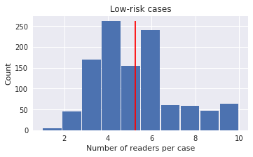
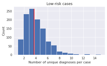
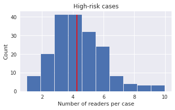
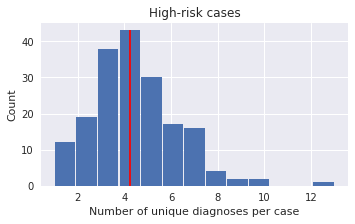
Figure 12: We plot the number of annotators per case and the number of unique conditions annotated by these annotators for low- (left) and high-risk (right) cases. Risk categories are based on the risk-level of the top-1 IRN condition as in previous work (Roy et al., 2022). Surprisingly, high-risk cases were annotated by, on average, less annotators while clearly yielding more unique conditions.

We use the de-identified dermatology dataset previously used in (Liu et al., 2020) which was collected from $17$ different sites across California and Hawaii. Each case in the dataset consists of up to $3$ RGB images, taken by medical assistants using consumer-grade digital cameras in a clinical environment. The images exhibit a large amount of variation in terms of affected anatomic location, background objects, resolution, perspective and lighting. Our dataset has patients with different skin types varying between Fitzpatrick scale of $1-6$. We resized each image to $448\times 448$ pixels for our training and evaluation purposes. The dataset consists of $16,225$ cases, where $12,335$ cases are used for model training, $1951$ cases for validation and $1939$ cases for test set. Note that in our dataset there are a few patients with multiple cases collected during repeated visits over the duration of the data collection process. For the data split, we ensured a patient-level split to avoid any bias. Furthermore, we ensured a similar distribution of skin conditions and risk categories. The latter corresponds to a classification of case outcomes for a given skin condition, i.e., each skin condition has been mapped to a risk category in low, medium and high. We operate on a label space of $419$ skin conditions similar to (Liu et al., 2020), following a long-tailed distribution. The dataset was labelled by US or Indian board certified dermatologists with $5-30$ years of experience. Annotation was conducted over a period of time in tandem to data collection between $2010-2018$. As a result, different cases were annotated by different dermatologists (see Figure 12 for statistics). Moreover, there are varying numbers of annotations per case but we made sure to have at least $3$ annotations per case.

C.1 Annotation details

All dermatologists were actively seeing patients in clinics and passed a certification test to ensure they were comfortable grading cases in our labeling tool. To provide the differential diagnoses, each annotator selected one or multiple conditions from the standardized Systematized Nomenclature of Medicine-Clinical Terms (SNOMED-CT) using a search-as-you-type interface, and assigned a confidence rating per condition. The conditions were later mapped to the 419 conditions as described previously (Liu et al., 2020). The confidence ratings were then used to rank conditions since confidence assignments are not comparable across dermatologists. As multiple conditions can obtain the same confidence ratings, this results in the partial rankings described in Section B. These rankings are the basis for our study and several prior works (Eng et al., 2019; Roy et al., 2021; Azizi et al., 2022). As the associated risk levels are of particular interest for analysis in prior work (Roy et al., 2021), it is important to highlight that different annotator annotations also correspond to different risk annotations. Note that risk is not specific to each case but rather based on a fixed condition to risk mapping.

C.2 Training details

As we have multiple images per case, we are dealing with a multi-instance classification task with $419$ labels. As we are dealing with limited training data, we use the BiT-L model (Kolesnikov et al., 2020), pre-trained on JFT dataset (Sun et al., 2017) containing large-scale natural images from the internet. The encoder provides a feature representation for each image instance in a case. This output is then passed through an instance level average pooling layer, which generates a common feature-map for all the instances for a given case. This is passed to a classification head through a drop-out layer. The classification head has an intermediate fully-connected hidden layer with $1024$-dimensions followed by a final classification with a softmax layer which provide probabilities for each of the $419$ classes. To keep model training process consistent to prior work (Liu et al., 2020; Roy et al., 2022), we use IRN as (soft) supervision in a cross-entropy loss. For data augmentation, we use horizontal and vertical flips, rotations, variations of brightness, contrast and saturation, and random Gaussian blurring. We use a Adam optimizer for training. Each model is trained for $10,000$ steps. Convergence of all the models were ensured on the validation set. We use a batch-size of $16$ cases for training. For each model, we select the final checkpoint based on the highest top-3 accuracy against the top-1 IRN ground truth label, consistent with previous work. We train a pool of 30 models by randomly varying the size of the ResNet architecture (depth $\times$ width: $101\times 3$, $101\times 1$, $50\times 3$, $152\times 2$, $152\times 4$), pre-logit dropout rate (keep probability: $0.5-0.7$) and learning rate ($10^{-6}-5\times 10^{-4}$). As model performance is not the focus of this work, we randomly selected four of these models for our experiments.

C.3 PL and PrIRN details

As detailed in Section B.4, for PL, we repeat annotators in order to simulate higher reliability. Specifically, corresponding to the x-axis in Figure 6, we evaluate 1, 2, 3, 5, and 10 repetitions. For PrIRN, we evaluate temperatures $\gamma=10,20,30,50,100$.

Appendix D Additional results

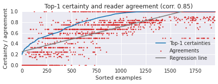
Figure 13: PL annotation certainty (blue) at medium reliability (see Figure 7) plotted with annotator agreement (red), see text for details. With a correlation coefficient of $0.85$, both measures are highly correlated, indicating that annotation certainty indeed captures the uncertainty induced by disagreement.

PL top-1 annotation certainty and agreement: Figure 13 correlates top-1 annotation certainty from PL (blue, at medium reliability corresponding to Figure 7) with annotator agreement (red). Here, agreement is computed as follows: For $R$ annotators, given a selected annotator $r$, we compute IRN plausibilities using all annotator opinions except those from $r$. We then check whether the top-1 IRN label is included in the conditions provided by annotator $r$. We then average across annotators $r\in[R]$. More formally:

$$\frac{1}{R}\sum_{r=1}^{R}\delta[\arg\max_{k\in[K]}\text{IRN}(k;b^{1},\ldots,b^{r-1},b^{r+1},\ldots,b^{R})\in\cup_{l=1}^{L_{r}-1}b^{r}_{l}],$$

where $L_{r}$ is the number of blocks in annotation provided by $r$, and we ignore $b^{r}_{L_{r}}$ since we use the last block to collect all unranked classes. We found high correlation between this notion of annotator agreement and our annotation certainty, as also highlighted by the gray regression line. This further highlights that our statistical aggregation model and the derived measure annotation certainty captures disagreement and the corresponding uncertainty well.

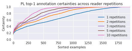
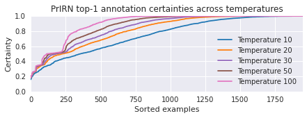
Figure 14: Top-1 annotation certainty for PL (left) and PrIRN across reliabilities. As detailed in the text, for PL, reliability is approximated by repeating annotations; for PrIRN, we can directly increase the corresponding temperature parameter.

Reliabity in PL and PrIRN: Figure 14 plots top-1 annotation certainty for PL and PrIRN across reliabilities. As detailed in Section B, reliability can be understood as the number of annotators in both cases. For PL, we explicitly repeat annotators as integrating a temperature into the statistical aggregation model makes sampling from the posterior infeasible; for PrIRN, in contrast, Section B.3 allows the direct use of a temperature. As indicated by Figure 6 (left), average annotation certainty increases with reliability. This suggests that annotation certainty increases across examples. However, this is not entirely true; we clearly see a saturating effect for at least 250 cases where higher reliability does not seem to increase annotation certainty. This further supports our observation that the observed disagreement for many cases is actually due to inherent uncertainty, i.e., these cases are inherently ambiguous for annotators.

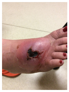
A0: {Pyoderma gangrenosum, Venous stasis ulcer}
A1: {Arterial ulcer, Calciphylaxis cutis}
A2: {Cellulitis}

Image and annotations

 

Plausibilities

 

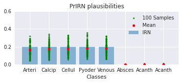
Pred.

Model A: $C_{\text{top-}3}=$
{Diabetic ulcer, Pyoderma Gangrenosum, Venous Stasis Ulcer}

Model D: $C_{\text{top-}3}=$
{Arterial ulcer, Cellulitis, Pyoderma Gangrenosum}

 

Eval.

Model A	PL	PrIRN
$\mathbb{E}_{p(\lambda|b,x)}\{\delta[Y_{\text{top-}1}(\lambda)\subset C_{\text{top-}k}(x)]\}$	$0.39$	$0.41$

Model D	PL	PrIRN
$\mathbb{E}_{p(\lambda|b,x)}\{\delta[Y_{\text{top-}1}(\lambda)\subset C_{\text{top-}k}(x)]\}$	$0.58$	$0.61$

 

Image and annotations

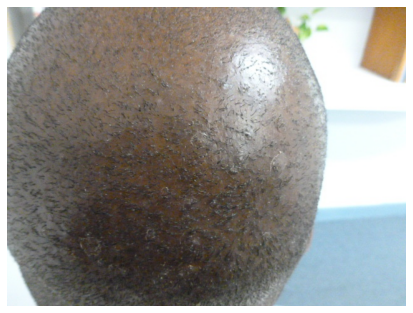
A0: {Dissecting cellulitis of scalp, Tinea} {Seborrheic dermatitis}
A1: {Acne keloidalis, Folliculitis decalvans}
A2: {Folliculitis}

 

Plausibilities

 

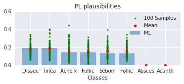
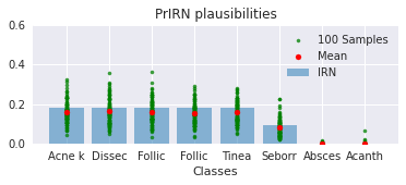
Pred.

Model A: $C_{\text{top-}3}=$
{Acne, Folliculitis, Folliculitis decalvans}

Model B: $C_{\text{top-}3}=$
{Acne keloidalis, Folliculitis, Folliculitis decalvans}

 

Eval.

Model A	PL	PrIRN
$\mathbb{E}_{p(\lambda|b,x)}\{\delta[Y_{\text{top-}1}(\lambda)\subset C_{\text{top-}k}(x)]\}$	$0.27$	$0.4$

Model B	PL	PrIRN
$\mathbb{E}_{p(\lambda|b,x)}\{\delta[Y_{\text{top-}1}(\lambda)\subset C_{\text{top-}k}(x)]\}$	$0.42$	$0.62$

Figure 15: Two additional qualitative results corresponding to cases with very low annotation certainty, following the presentation of Figure 5.

Qualitative results: Figure 15 shows two additional qualitative cases where we observed very low annotation certainty (i.e., in Figure 14, these likely lie on the very left). In both cases, annotators provided widely different conditions, leading PL and PrIRN to distribute the plausibility mass nearly equally across the annotated conditions. Again, this also has significant impact on evaluating the top-3 prediction sets of our classifiers.

References

- Abercrombie et al. (2023) G. Abercrombie, V. Rieser, and D. Hovy. Consistency is key: Disentangling label variation in natural language processing with intra-annotator agreement. arXiv.org, abs/2301.10684, 2023.
- Angluin and Laird (1987) D. Angluin and P. D. Laird. Learning from noisy examples. Machine Learning, 2(4):343–370, 1987.
- Aroyo and Welty (2014) L. Aroyo and C. Welty. The three sides of crowdtruth. Journal of Human Computation, 1(1):31–44, 2014.
- Aroyo and Welty (2015) L. Aroyo and C. Welty. Truth is a lie: Crowd truth and the seven myths of human annotation. AI Magazine, 36(1):15–24, 2015.
- Azizi et al. (2022) S. Azizi, L. Culp, J. Freyberg, B. Mustafa, S. Baur, S. Kornblith, T. Chen, P. MacWilliams, S. S. Mahdavi, E. Wulczyn, B. Babenko, M. Wilson, A. Loh, P. C. Chen, Y. Liu, P. Bavishi, S. M. McKinney, J. Winkens, A. G. Roy, Z. Beaver, F. Ryan, J. Krogue, M. Etemadi, U. Telang, Y. Liu, L. Peng, G. S. Corrado, D. R. Webster, D. J. Fleet, G. E. Hinton, N. Houlsby, A. Karthikesalingam, M. Norouzi, and V. Natarajan. Robust and efficient medical imaging with self-supervision. arXiv.org, abs/2205.09723, 2022.
- Baan et al. (2022) J. Baan, W. Aziz, B. Plank, and R. Fernández. Stop measuring calibration when humans disagree. arXiv.org, abs/2210.16133, 2022.
- Bachrach et al. (2012) Y. Bachrach, T. Graepel, T. Minka, and J. Guiver. How to grade a test without knowing the answers - A bayesian graphical model for adaptive crowdsourcing and aptitude testing. In Proc. of the International Conference on Machine Learning (ICML), 2012.
- Bakker et al. (2022) M. A. Bakker, M. J. Chadwick, H. Sheahan, M. H. Tessler, L. Campbell-Gillingham, J. Balaguer, N. McAleese, A. Glaese, J. Aslanides, M. M. Botvinick, and C. Summerfield. Fine-tuning language models to find agreement among humans with diverse preferences. In Advances in Neural Information Processing Systems (NeurIPS), 2022.
- Basile et al. (2021) V. Basile, M. Fell, T. Fornaciari, D. Hovy, S. Paun, B. Plank, M. Poesio, and A. Uma. We need to consider disagreement in evaluation. In Proceedings of the 1st Workshop on Benchmarking: Past, Present and Future, 2021.
- Beigman and Klebanov (2009) E. Beigman and B. B. Klebanov. Learning with annotation noise. In Proc. of the Annual Meeting of the Association for Computational Linguistics (ACL). The Association for Computer Linguistics, 2009.
- Belz et al. (2023) A. Belz, C. Thomson, E. Reiter, G. Abercrombie, J. M. Alonso-Moral, M. Arvan, J. C. K. Cheung, M. Cieliebak, E. Clark, K. van Deemter, T. Dinkar, O. Dusek, S. Eger, Q. Fang, A. Gatt, D. Gkatzia, J. González-Corbelle, D. Hovy, M. Hürlimann, T. Ito, J. D. Kelleher, F. Klubicka, H. Lai, C. van der Lee, E. van Miltenburg, Y. Li, S. Mahamood, M. Mieskes, M. Nissim, N. Parde, O. Plátek, V. Rieser, P. M. Romero, J. R. Tetreault, A. Toral, X. Wan, L. Wanner, L. Watson, and D. Yang. Missing information, unresponsive authors, experimental flaws: The impossibility of assessing the reproducibility of previous human evaluations in NLP. arXiv.org, abs/2305.01633, 2023.
- Bhattacharya et al. (2019) N. Bhattacharya, Q. Li, and D. Gurari. Why does a visual question have different answers? In Proc. of the IEEE International Conference on Computer Vision (ICCV), 2019.
- Braylan et al. (2022) A. Braylan, O. Alonso, and M. Lease. Measuring annotator agreement generally across complex structured, multi-object, and free-text annotation tasks. In Proc. of the International World Wide Web Conference (WWW), 2022.
- Cabitza et al. (2020) F. Cabitza, A. Campagner, D. Albano, A. Aliprandi, A. Bruno, V. Chianca, A. Corazza, F. Di Pietto, A. Gambino, S. Gitto, et al. The elephant in the machine: Proposing a new metric of data reliability and its application to a medical case to assess classification reliability. Applied Sciences, 10(11):4014, 2020.
- Caron and Doucet (2010) F. Caron and A. Doucet. Efficient bayesian inference for generalized bradley–terry models. Journal of Computational and Graphical Statistics, 21:174 – 196, 2010.
- Carvalho and Larson (2013) A. Carvalho and K. Larson. A consensual linear opinion pool. In Proc. of the International Joint Conference on Artificial Intelligence (IJCAI), 2013.
- Chen et al. (2019a) P. Chen, B. Liao, G. Chen, and S. Zhang. Understanding and utilizing deep neural networks trained with noisy labels. In Proc. of the International Conference on Machine Learning (ICML), 2019a.
- Chen et al. (2021) P. Chen, J. Ye, G. Chen, J. Zhao, and P. Heng. Robustness of accuracy metric and its inspirations in learning with noisy labels. In Thirty-Fifth AAAI Conference on Artificial Intelligence, AAAI 2021, Thirty-Third Conference on Innovative Applications of Artificial Intelligence, IAAI 2021, The Eleventh Symposium on Educational Advances in Artificial Intelligence, EAAI 2021, Virtual Event, February 2-9, 2021, pages 11451–11461. AAAI Press, 2021. URL https://ojs.aaai.org/index.php/AAAI/article/view/17364.
- Chen et al. (2019b) Q. Chen, J. Bragg, L. B. Chilton, and D. S. Weld. Cicero: Multi-turn, contextual argumentation for accurate crowdsourcing. In Proc. of the Conference on Human Factors in Computing Systems, 2019b.
- Chu et al. (2021) Z. Chu, J. Ma, and H. Wang. Learning from crowds by modeling common confusions. In Proc. of the Conference on Artificial Intelligence (AAAI), 2021.
- Cohen (1960) J. Cohen. A coefficient of agreement for nominal scales. Educational and Psychological Measurement, 20(1):37–46, 1960.
- Collins et al. (2022) K. M. Collins, U. Bhatt, and A. Weller. Eliciting and learning with soft labels from every annotator. In Proc. of the AAAI Conference on Human Computation and Crowdsourcing (HCOMP), 2022.
- Cour et al. (2011) T. Cour, B. Sapp, and B. Taskar. Learning from partial labels. Journal of Machine Learning Research (JMLR), 12, 2011.
- Davani et al. (2022) A. M. Davani, M. Díaz, and V. Prabhakaran. Dealing with disagreements: Looking beyond the majority vote in subjective annotations. Transactions of the Association for Computational Linguistics (TACL), 10:92–110, 2022.
- Dawid and Skene (1979) A. P. Dawid and A. M. Skene. Maximum likelihood estimation of observer error-rates using the em algorithm. Journal of the Royal Statistical Society (JRSS), 28(1):20–28, 1979.
- de Marneffe et al. (2012) M. de Marneffe, C. D. Manning, and C. Potts. Did it happen? the pragmatic complexity of veridicality assessment. Computational Linguistics, 2012.
- Dong et al. (2009) X. L. Dong, L. Berti-Équille, and D. Srivastava. Integrating conflicting data: The role of source dependence. Proc. of the VLDB Endowment, 2(1):550–561, 2009.
- Drapeau et al. (2016) R. Drapeau, L. Chilton, J. Bragg, and D. Weld. Microtalk: Using argumentation to improve crowdsourcing accuracy. In Proc. of the AAAI Conference on Human Computation and Crowdsourcing (HCOMP), volume 4, 2016.
- Duggan et al. (2021) G. E. Duggan, J. J. Reicher, Y. Liu, D. Tse, and S. Shetty. Improving reference standards for validation of ai-based radiography. The British Journal of Radiology, 94, 2021.
- Dumitrache et al. (2019) A. Dumitrache, L. Aroyo, and C. Welty. A crowdsourced frame disambiguation corpus with ambiguity. In J. Burstein, C. Doran, and T. Solorio, editors, Proc. of the Conference of the North American Chapter of the Association for Computational Linguistics: Human Language Technologies (NAACL-HLT), 2019.
- Eng et al. (2019) C. Eng, Y. Liu, and R. Bhatnagar. Measuring clinician–machine agreement in differential diagnoses for dermatology. British Journal of Dermatology, 182, 2019.
- Esfandarani and Milanfar (2018) H. T. Esfandarani and P. Milanfar. NIMA: neural image assessment. IEEE Trans. on Image Processing (TIP), 27(8):3998–4011, 2018.
- Fagin et al. (2003) R. Fagin, R. Kumar, and D. Sivakumar. Comparing top k lists. SIAM Journal on Discrete Mathematics (SIDMA), 17(1):134–160, 2003.
- Fagin et al. (2004) R. Fagin, R. Kumar, M. Mahdian, D. Sivakumar, and E. Vee. Comparing and aggregating rankings with ties. In Proc. of the ACM SIGACT-SIGMOD-SIGART Symposium on Principles of Database Systems (PODS), 2004.
- Feinstein and Cicchetti (1990) A. R. Feinstein and D. V. Cicchetti. High agreement but low kappa: I. the problems of two paradoxes. Journal of Clinical Epidemiology, 43 6:543–9, 1990.
- Field et al. (2021) A. Field, S. L. Blodgett, Z. Waseem, and Y. Tsvetkov. A survey of race, racism, and anti-racism in NLP. In Proc. of the Annual Meeting of the Association for Computational Linguistics (ACL), 2021.
- Fleiss et al. (2003) J. L. Fleiss, B. Levin, and M. C. Paik. Statistical methods for rates and proportions, 3rd edition. Wiley, 2003.
- Francois et al. (2012) Francois, Y. W. Teh, and T. B. Murphy. Bayesian nonparametric plackett-luce models for the analysis of clustered ranked data. arXiv.org, abs/1211.5037, 2012.
- Freeman et al. (2021) B. Freeman, N. Hammel, S. Phene, A. Huang, R. Ackermann, O. Kanzheleva, M. Hutson, C. Taggart, Q. Duong, and R. Sayres. Iterative quality control strategies for expert medical image labeling. In Proc. of the AAAI Conference on Human Computation and Crowdsourcing (HCOMP), pages 60–71, 2021.
- Gao et al. (2017) B.-B. Gao, C. Xing, C.-W. Xie, J. Wu, and X. Geng. Deep label distribution learning with label ambiguity. IEEE Trans. on Image Processing (TIP), 26(6):2825–2838, 2017.
- Gaunt et al. (2016) A. Gaunt, D. Borsa, and Y. Bachrach. Training deep neural nets to aggregate crowdsourced responses. In Proc. of the Conference on Uncertainty in Artificial Intelligence (UAI), volume 242251, 2016.
- Gordon et al. (2021) M. L. Gordon, K. Zhou, K. Patel, T. Hashimoto, and M. S. Bernstein. The disagreement deconvolution: Bringing machine learning performance metrics in line with reality. In Proc. of the Conference on Human Factors in Computing Systems, 2021.
- Gordon et al. (2022) M. L. Gordon, M. S. Lam, J. S. Park, K. Patel, J. T. Hancock, T. Hashimoto, and M. S. Bernstein. Jury learning: Integrating dissenting voices into machine learning models. In Proc. of the Conference on Human Factors in Computing Systems, 2022.
- Guan et al. (2018) M. Y. Guan, V. Gulshan, A. M. Dai, and G. E. Hinton. Who said what: Modeling individual labelers improves classification. In Proc. of the Conference on Artificial Intelligence (AAAI), 2018.
- Hendrycks et al. (2018) D. Hendrycks, M. Mazeika, D. Wilson, and K. Gimpel. Using trusted data to train deep networks on labels corrupted by severe noise. In Advances in Neural Information Processing Systems (NeurIPS), 2018.
- Hüllermeier and Beringer (2005) E. Hüllermeier and J. Beringer. Learning from ambiguously labeled examples. In Proc. of the International Symposium on Intelligent Data Analysis (IDA), 2005.
- Hunter (2003) D. R. Hunter. Mm algorithms for generalized bradley-terry models. The Annals of Statistics, 32:384–406, 2003.
- Jain et al. (2021) A. Jain, D. H. Way, V. Gupta, Y. Gao, G. de Oliveira Marinho, J. Hartford, R. Sayres, K. Kanada, C. Eng, K. Nagpal, K. Desalvo, G. S. Corrado, L. H. Peng, D. R. Webster, R. C. Dunn, D. Coz, S. J. Huang, Y. Liu, P. Bui, and Y. Liu. Development and assessment of an artificial intelligence-based tool for skin condition diagnosis by primary care physicians and nurse practitioners in teledermatology practices. Journal of the American Medical Association (JAMA), 4 4, 2021.
- Kearns (1998) M. J. Kearns. Efficient noise-tolerant learning from statistical queries. Journal of the ACM, 45(6):983–1006, 1998.
- Kearns and Li (1993) M. J. Kearns and M. Li. Learning in the presence of malicious errors. SIAM Journal on Computing, 22(4):807–837, 1993.
- Kiela et al. (2020) D. Kiela, H. Firooz, A. Mohan, V. Goswami, A. Singh, P. Ringshia, and D. Testuggine. The hateful memes challenge: Detecting hate speech in multimodal memes. In Advances in Neural Information Processing Systems (NeurIPS), 2020.
- Kolesnikov et al. (2020) A. Kolesnikov, L. Beyer, X. Zhai, J. Puigcerver, J. Yung, S. Gelly, and N. Houlsby. Big transfer (bit): General visual representation learning. In A. Vedaldi, H. Bischof, T. Brox, and J. Frahm, editors, Proc. of the European Conference on Computer Vision (ECCV), 2020.
- Kovashka et al. (2016) A. Kovashka, O. Russakovsky, L. Fei-Fei, and K. Grauman. Crowdsourcing in computer vision. Foundations and Trends in Computer Graphics and Vision, 10(3):177–243, 2016.
- Krizhevsky (2009) A. Krizhevsky. Learning multiple layers of features from tiny images. Technical report, University of Toronto, 2009.
- Kumar and Vassilvitskii (2010) R. Kumar and S. Vassilvitskii. Generalized distances between rankings. In Proc. of the International World Wide Web Conference (WWW), 2010.
- Landis and Koch (1977) J. R. Landis and G. G. Koch. The measurement of observer agreement for categorical data. Biometrics, pages 159–174, 1977.
- Lawrence and Schölkopf (2001) N. D. Lawrence and B. Schölkopf. Estimating a kernel fisher discriminant in the presence of label noise. In Proc. of the International Conference on Machine Learning (ICML), 2001.
- Leonardelli et al. (2021) E. Leonardelli, S. Menini, A. P. Aprosio, M. Guerini, and S. Tonelli. Agreeing to disagree: Annotating offensive language datasets with annotators’ disagreement. In Proc. of the Conference on Empirical Methods in Natural Language Processing, 2021.
- Leonardelli et al. (2023) E. Leonardelli, A. Uma, G. Abercrombie, D. Almanea, V. Basile, T. Fornaciari, B. Plank, V. Rieser, and M. Poesio. Semeval-2023 task 11: Learning with disagreements (lewidi). arXiv.org, abs/2304.14803, 2023.
- Li et al. (2012) X. Li, X. L. Dong, K. Lyons, W. Meng, and D. Srivastava. Truth finding on the deep web: Is the problem solved? Proc. of the VLDB Endowment, 6(2):97–108, 2012.
- Liu et al. (2020) Y. Liu, A. Jain, C. Eng, D. H. Way, K. Lee, P. Bui, K. Kanada, G. de Oliveira Marinho, J. Gallegos, S. Gabriele, V. Gupta, N. Singh, V. Natarajan, R. Hofmann-Wellenhof, G. S. Corrado, L. H. Peng, D. R. Webster, D. Ai, S. Huang, Y. Liu, R. C. Dunn, and D. Coz. A deep learning system for differential diagnosis of skin diseases. Nature Medicine, 26:900–908, 2020.
- Lovchinsky et al. (2020) I. Lovchinsky, A. Daks, I. Malkin, P. Samangouei, A. Saeedi, Y. Liu, S. Sankaranarayanan, T. Gafner, B. Sternlieb, P. Maher, and N. Silberman. Discrepancy ratio: Evaluating model performance when even experts disagree on the truth. In Proc. of the International Conference on Learning Representations (ICLR), 2020.
- Lu et al. (2014) X. Lu, Z. Lin, H. Jin, J. Yang, and J. Z. Wang. RAPID: rating pictorial aesthetics using deep learning. In Proc. of the ACM International Conference on Multimedia (MM), 2014.
- Luce (2012) R. D. Luce. Individual choice behavior: A theoretical analysis. Courier Corporation, 2012.
- Maier-Hein et al. (2018) L. Maier-Hein, M. Eisenmann, A. Reinke, S. Onogur, M. Stankovic, P. Scholz, T. Arbel, H. Bogunović, A. P. Bradley, A. Carass, C. Feldmann, A. F. Frangi, P. M. Full, B. van Ginneken, A. Hanbury, K. Honauer, M. Kozubek, B. A. Landman, K. März, O. Maier, K. Maier-Hein, B. H. Menze, H. Müller, P. Neher, W. J. Niessen, N. M. Rajpoot, G. C. Sharp, K. Sirinukunwattana, S. Speidel, C. Stock, D. Stoyanov, A. A. Taha, F. van der Sommen, C.-W. Wang, M.-A. Weber, G. Zheng, P. Jannin, and A. Kopp-Schneider. Why rankings of biomedical image analysis competitions should be interpreted with care. Nature Communications, 9, 2018.
- McHugh (2012) M. L. McHugh. Interrater reliability: the kappa statistic. Biochemia Medica, 22:276 – 282, 2012.
- Medeiros et al. (2023) F. A. Medeiros, T. Lee, A. A. Jammal, L. A. Al-Aswad, M. B. Eydelman, and J. S. Schuman. The definition of glaucomatous optic neuropathy in artificial intelligence research and clinical applications. Ophthalmology. Glaucoma, 2023.
- Murray et al. (2012) N. Murray, L. Marchesotti, and F. Perronnin. AVA: A large-scale database for aesthetic visual analysis. In Proc. of the IEEE Conference on Computer Vision and Pattern Recognition (CVPR), 2012.
- Nguyen and Caruana (2008) N. Nguyen and R. Caruana. Classification with partial labels. In Proc. of the ACM International Conference on Knowledge Discovery & Data Mining, 2008.
- Nie et al. (2020) Y. Nie, X. Zhou, and M. Bansal. What can we learn from collective human opinions on natural language inference data? In Proc. of the Conference on Empirical Methods in Natural Language Processing, 2020.
- Northcutt et al. (2019) C. G. Northcutt, L. Jiang, and I. L. Chuang. Confident learning: Estimating uncertainty in dataset labels. arXiv.org, abs/1911.00068, 2019.
- Northcutt et al. (2021) C. G. Northcutt, A. Athalye, and J. Mueller. Pervasive label errors in test sets destabilize machine learning benchmarks. In Advances in Neural Information Processing Systems (NeurIPS) Workshops, 2021.
- Oyen et al. (2022) D. Oyen, M. Kucer, N. Hengartner, and H. S. Singh. Robustness to label noise depends on the shape of the noise distribution in feature space. arXiv.org, abs/2206.01106, 2022.
- Pavlick and Kwiatkowski (2019) E. Pavlick and T. Kwiatkowski. Inherent disagreements in human textual inferences. Transactions of the Association for Computational Linguistics (TACL), 7:677–694, 2019.
- Peterson et al. (2019) J. C. Peterson, R. M. Battleday, T. L. Griffiths, and O. Russakovsky. Human uncertainty makes classification more robust. In Proc. of the IEEE International Conference on Computer Vision (ICCV), 2019.
- Pham et al. (2017) A. T. Pham, R. Raich, and X. Z. Fern. Dynamic programming for instance annotation in multi-instance multi-label learning. IEEE Transactions on Pattern Analysis and Machine Intelligence, 39(12):2381–2394, 2017.
- Phene et al. (2019) S. Phene, R. C. Dunn, N. Hammel, Y. Liu, J. Krause, N. Kitade, M. Schaekermann, R. Sayres, D. J. Wu, A. Bora, C. Semturs, A. Misra, A. E. Huang, A. Spitze, F. A. Medeiros, A. Y. Maa, M. Gandhi, G. S. Corrado, L. H. Peng, and D. R. Webster. Deep learning and glaucoma specialists: The relative importance of optic disc features to predict glaucoma referral in fundus photographs. Ophthalmology, 2019.
- Plackett (1975) R. L. Plackett. The analysis of permutations. Journal of The Royal Statistical Society Series C-applied Statistics, 24:193–202, 1975.
- Plank (2022) B. Plank. The ’problem’ of human label variation: On ground truth in data, modeling and evaluation. arXiv.org, abs/2211.02570, 2022.
- Powers (2012) D. M. W. Powers. The problem with kappa. In Proc. of the Conference of the European Chapter of the Association for Computational Linguistics (EACL), pages 345–355, 2012.
- Pradhan et al. (2022) V. K. Pradhan, M. Schaekermann, and M. Lease. In search of ambiguity: A three-stage workflow design to clarify annotation guidelines for crowd workers. Frontiers Artificial Intelligence, 5:828187, 2022.
- Raghu et al. (2019) M. Raghu, K. Blumer, R. Sayres, Z. Obermeyer, B. Kleinberg, S. Mullainathan, and J. Kleinberg. Direct uncertainty prediction for medical second opinions. In Proc. of the International Conference on Machine Learning (ICML), 2019.
- Reidsma and op den Akker (2008) D. Reidsma and R. op den Akker. Exploiting ’subjective’ annotations. In Proc. of the Annual Meeting of the Association for Computational Linguistics (ACL), 2008.
- Rodrigues and Pereira (2018) F. Rodrigues and F. C. Pereira. Deep learning from crowds. In Proc. of the Conference on Artificial Intelligence (AAAI), 2018.
- Röttger et al. (2021) P. Röttger, B. Vidgen, D. Nguyen, Z. Waseem, H. Z. Margetts, and J. B. Pierrehumbert. Hatecheck: Functional tests for hate speech detection models. In Proc. of the Annual Meeting of the Association for Computational Linguistics (ACL), 2021.
- Röttger et al. (2022) P. Röttger, B. Vidgen, D. Hovy, and J. B. Pierrehumbert. Two contrasting data annotation paradigms for subjective NLP tasks. In Proc. of the Conference of the North American Chapter of the Association for Computational Linguistics: Human Language Technologies (NAACL-HLT), 2022.
- Roy et al. (2021) A. G. Roy, J. Ren, S. Azizi, A. Loh, V. Natarajan, B. Mustafa, N. Pawlowski, J. Freyberg, Y. Liu, Z. Beaver, N. S. Vo, P. Bui, S. Winter, P. MacWilliams, G. S. Corrado, U. Telang, Y. Liu, T. Cemgil, A. Karthikesalingam, B. Lakshminarayanan, and J. Winkens. Does your dermatology classifier know what it doesn’t know? detecting the long-tail of unseen conditions. arXiv.org, abs/2104.03829, 2021.
- Roy et al. (2022) A. G. Roy, J. Ren, S. Azizi, A. Loh, V. Natarajan, B. Mustafa, N. Pawlowski, J. Freyberg, Y. Liu, Z. Beaver, N. Vo, P. Bui, S. Winter, P. MacWilliams, G. S. Corrado, U. Telang, Y. Liu, A. T. Cemgil, A. Karthikesalingam, B. Lakshminarayanan, and J. Winkens. Does your dermatology classifier know what it doesn’t know? detecting the long-tail of unseen conditions. Medical Image Analysis, 75:102274, 2022.
- Russakovsky et al. (2015) O. Russakovsky, J. Deng, H. Su, J. Krause, S. Satheesh, S. Ma, Z. Huang, A. Karpathy, A. Khosla, M. S. Bernstein, A. C. Berg, and F. Li. Imagenet large scale visual recognition challenge. International Journal of Computer Vision (IJCV), 115(3):211–252, 2015.
- Sakai (2013) T. Sakai. Metrics, statistics, tests. In PROMISE Winter School, 2013.
- Sandri et al. (2023) M. Sandri, E. Leonardelli, S. Tonelli, and E. Jezek. Why don’t you do it right? analysing annotators’ disagreement in subjective tasks. In Proc. of the Conference of the European Chapter of the Association for Computational Linguistics (EACL), 2023.
- Schaekermann (2020) M. Schaekermann. Human-AI Interaction in the Presence of Ambiguity: From Deliberation-based Labeling to Ambiguity-aware AI. Ph.d. thesis, University of Waterloo, 2020.
- Schaekermann et al. (2016) M. Schaekermann, E. Law, A. C. Williams, and W. Callaghan. Resolvable vs. irresolvable ambiguity: A new hybrid framework for dealing with uncertain ground truth. In SIGCHI Workshop on Human-Centered Machine Learning, volume 2016, 2016.
- Schaekermann et al. (2019a) M. Schaekermann, G. Beaton, M. Habib, A. Lim, K. Larson, and E. Law. Understanding expert disagreement in medical data analysis through structured adjudication. Proc. ACM Hum. Comput. Interact., 3:76:1–76:23, 2019a.
- Schaekermann et al. (2019b) M. Schaekermann, N. Hammel, M. Terry, T. K. Ali, Y. Liu, B. Basham, B. Campana, W. Chen, X. Ji, J. Krause, et al. Remote tool-based adjudication for grading diabetic retinopathy. Translational Vision Science & Technology, 8(6), 2019b.
- Schaekermann et al. (2020a) M. Schaekermann, G. Beaton, E. Sanoubari, A. Lim, K. Larson, and E. Law. Ambiguity-aware AI assistants for medical data analysis. In Proc. of the Conference on Human Factors in Computing Systems, pages 1–14. ACM, 2020a.
- Schaekermann et al. (2020b) M. Schaekermann, C. J. Cai, A. E. Huang, and R. Sayres. Expert discussions improve comprehension of difficult cases in medical image assessment. In Proc. of the Conference on Human Factors in Computing Systems, 2020b.
- Sculley (2007) D. Sculley. Rank aggregation for similar items. In Proc. of the SIAM International Conference on Data Mining (SDM), 2007.
- Sheng et al. (2008) V. S. Sheng, F. J. Provost, and P. G. Ipeirotis. Get another label? improving data quality and data mining using multiple, noisy labelers. In Proc. of the ACM International Conference on Knowledge Discovery & Data Mining, 2008.
- Shieh (1998) G. S. Shieh. A weighted kendall’s tau statistic. Statistics & Probability Letters, 39(1):17–24, 1998.
- Silver et al. (2021) I. Silver, B. A. Mellers, and P. E. Tetlock. Wise teamwork: Collective confidence calibration predicts the effectiveness of group discussion. Journal of Experimental Social Psychology, 96, 2021.
- Smyth et al. (1994) P. Smyth, U. M. Fayyad, M. C. Burl, P. Perona, and P. Baldi. Inferring ground truth from subjective labelling of venus images. In Advances in Neural Information Processing Systems (NeurIPS), 1994.
- Snow et al. (2008) R. Snow, B. O’Connor, D. Jurafsky, and A. Y. Ng. Cheap and fast - but is it good? evaluating non-expert annotations for natural language tasks. In Proc. of the Conference on Empirical Methods in Natural Language Processing, 2008.
- Sorokin and Forsyth (2008) A. Sorokin and D. A. Forsyth. Utility data annotation with amazon mechanical turk. In Proc. of the IEEE Conference on Computer Vision and Pattern Recognition (CVPR) Workshops, 2008.
- Sun et al. (2017) C. Sun, A. Shrivastava, S. Singh, and A. Gupta. Revisiting unreasonable effectiveness of data in deep learning era. In Proc. of the IEEE International Conference on Computer Vision (ICCV), 2017.
- Tanno et al. (2019) R. Tanno, A. Saeedi, S. Sankaranarayanan, D. C. Alexander, and N. Silberman. Learning from noisy labels by regularized estimation of annotator confusion. In Proc. of the IEEE Conference on Computer Vision and Pattern Recognition (CVPR), 2019.
- Tian et al. (2019) T. Tian, J. Zhu, and Y. Qiaoben. Max-margin majority voting for learning from crowds. IEEE Transactions on Pattern Analysis and Machine Intelligence, 41(10):2480–2494, 2019.
- Uma et al. (2021) A. Uma, T. Fornaciari, D. Hovy, S. Paun, B. Plank, and M. Poesio. Learning from disagreement: A survey. Journal of Artifical Intelligence Research, 72:1385–1470, 2021.
- Uma et al. (2022) A. Uma, D. Almanea, and M. Poesio. Scaling and disagreements: Bias, noise, and ambiguity. Frontiers in Artifical Intelligence, 5, 2022.
- Vigna (2015) S. Vigna. A weighted correlation index for rankings with ties. In Proc. of the International World Wide Web Conference (WWW), 2015.
- Vitsakis et al. (2023) N. Vitsakis, A. Parekh, T. Dinkar, G. Abercrombie, I. Konstas, and V. Rieser. ilab at semeval-2023 task 11 le-wi-di: Modelling disagreement or modelling perspectives? arXiv.org, abs/2305.06074, 2023.
- Wang et al. (2012) D. Wang, L. M. Kaplan, H. K. Le, and T. F. Abdelzaher. On truth discovery in social sensing: a maximum likelihood estimation approach. In Proc. of the International Conference on Information Processing in Sensor Networks IPSN, 2012.
- Wang et al. (2022) H. Wang, R. Xiao, Y. Li, L. Feng, G. Niu, G. Chen, and J. Zhao. Pico: Contrastive label disambiguation for partial label learning. In Proc. of the International Conference on Learning Representations (ICLR), 2022.
- Warby et al. (2014) S. C. Warby, S. L. Wendt, P. Welinder, E. G. Munk, O. Carrillo, H. B. Sorensen, P. Jennum, P. E. Peppard, P. Perona, and E. Mignot. Sleep-spindle detection: crowdsourcing and evaluating performance of experts, non-experts and automated methods. Nature methods, 11(4):385–392, 2014.
- Webber et al. (2010) W. Webber, A. Moffat, and J. Zobel. A similarity measure for indefinite rankings. ACM Transactions on Information Systems (TOIS), 28(4):20:1–20:38, 2010.
- Welinder and Perona (2010) P. Welinder and P. Perona. Online crowdsourcing: Rating annotators and obtaining cost-effective labels. In Proc. of the IEEE Conference on Computer Vision and Pattern Recognition (CVPR), 2010.
- Welinder et al. (2010) P. Welinder, S. Branson, S. J. Belongie, and P. Perona. The multidimensional wisdom of crowds. In Advances in Neural Information Processing Systems (NeurIPS), 2010.
- Wu and Crestani (2003) S. Wu and F. Crestani. Methods for ranking information retrieval systems without relevance judgments. In Proc. of the ACM Symposium on Applied Computing (SAC), 2003.
- Wulczyn et al. (2017) E. Wulczyn, N. Thain, and L. Dixon. Wikipedia Talk Labels: Personal Attacks. https://figshare.com/articles/dataset/Wikipedia_Talk_Labels_Personal_Attacks/4054689/6, 2017.
- Yan et al. (2014) Y. Yan, R. Rosales, G. Fung, S. Ramanathan, and J. G. Dy. Learning from multiple annotators with varying expertise. Machine Learning, 95(3):291–327, 2014.
- Yin et al. (2008) X. Yin, J. Han, and P. S. Yu. Truth discovery with multiple conflicting information providers on the web. IEEE Transactions on Knowledge and Data Engineering, 20(6):796–808, 2008.
- Zhang et al. (2022) J. Zhang, Y. Wang, and C. Scott. Learning from label proportions by learning with label noise. arXiv.org, abs/2203.02496, 2022.
- Zhang et al. (2020) L. Zhang, R. Tanno, M. Xu, C. Jin, J. Jacob, O. Ciccarelli, F. Barkhof, and D. C. Alexander. Disentangling human error from the ground truth in segmentation of medical images. arXiv.org, abs/2007.15963, 2020.
- Zhao et al. (2012) B. Zhao, B. I. P. Rubinstein, J. Gemmell, and J. Han. A bayesian approach to discovering truth from conflicting sources for data integration. Proc. of the VLDB Endowment, 5(6):550–561, 2012.
- Zheng et al. (2017) Y. Zheng, G. Li, Y. Li, C. Shan, and R. Cheng. Truth inference in crowdsourcing: Is the problem solved? Proc. of the VLDB Endowment, 10(5):541–552, 2017.