Beyond Known Reality: Exploiting Counterfactual Explanations for Medical Research

Abstract

The field of explainability in artificial intelligence (AI) has witnessed a growing number of studies and increasing scholarly interest. However, the lack of human-friendly and individual interpretations in explaining the outcomes of machine learning algorithms has significantly hindered the acceptance of these methods by clinicians in their research and clinical practice. To address this issue, our study uses counterfactual explanations to explore the applicability of "what if?" scenarios in medical research. Our aim is to expand our understanding of magnetic resonance imaging (MRI) features used for diagnosing pediatric posterior fossa brain tumors beyond existing boundaries. In our case study, the proposed concept provides a novel way to examine alternative decision-making scenarios that offer personalized and context-specific insights, enabling the validation of predictions and clarification of variations under diverse circumstances. Additionally, we explore the potential use of counterfactuals for data augmentation and evaluate their feasibility as an alternative approach in our medical research case. The results demonstrate the promising potential of using counterfactual explanations to enhance acceptance of AI-driven methods in clinical research.

Keywords counterfactuals  $\cdot$ pediatric brain tumors  $\cdot$ magnetic resonance imaging  $\cdot$ explainable AI

1 Introduction

As we incorporate automated decision-making systems into the real world, explainability and accountability questions become increasingly important [1]. In some fields, such as medicine and healthcare, ignoring or failing to address such a challenge can seriously limit the adoption of computer-based systems that rely on machine learning (ML) and computational intelligence methods for data analysis in real-world applications [2, 3, 4]. Previous research in eXplainable Artificial Intelligence (XAI) has primarily focused on developing techniques to interpret decisions made by black box ML models. For instance, widely used approaches such as local interpretable model-agnostic explanations (LIME) [5] and shapley additive explanations (SHAP) [6] offer attribution-based explanations to interpret ML models. These methods can assist computer scientists and ML experts in understanding the reasoning behind the predictions made by AI models. However, end-users, including clinicians and patients, may be more interested in understanding the practical implications of the ML model’s predictions in relation to themselves, rather than solely focusing on how the models arrived at their predictions. For example, patients’ primary concern lies not only in obtaining information about their illness but also in seeking guidance on how to regain their health. Understanding the decision-making process of either the doctor or the ML model is of lesser importance to them.

Counterfactual explanations [7, 8] are a form of model-agnostic interpretation technique that identifies the minimal changes needed in input features to yield a different output, aligned with a specific desired outcome. This approach holds promise in enhancing the data synthesize and for answering causal questions [9, 10], and interpretability of AI models by offering deeper insights into their decision-making processes [11, 12, 13]. Our proposed approach aims to uncover the underlying reasons for the observed relationships between MRI features, going beyond just generating actionable outcomes for individual patients. Through counterfactual explanations, previously unseen decisions within the decision space can be brought to light. Numerous questions can be explored, such as how to determine the modifications required to transform a patient’s diagnosis from one tumor subtype to another. Initially, posing such a question may seem nonsensical and illogical since an individual’s actual tumor type cannot be magically altered. However, considering the challenge of distinguishing these two tumor types in clinical settings, asking such a question can effectively demonstrate which features are more informative in differentiating tumor types. Counterfactual explanations enable us to identify the characteristics that distinguish two patient types with the smallest changes in features. Consequently, a deeper understanding of the interactions between MRI features and tumors can be gained; unveiling previously undisclosed outcomes that may be concealed in existing ML studies.

Furthermore, we have identified a potential contribution to clinical practice whereby a new patient with only MRI data available can have their tumor type estimated using a counterfactual approach, prior to receiving histopathological results. Since there is no prior label available for the patient, they are given an "unknown" label and the counterfactual approach is used for each tumor type, allowing estimation of the tumor type with the lowest distance and smallest change in features. While this approach shares similarities with ML, the crucial distinction lies in retaining information about the reasoning behind the estimated tumor type and its corresponding feature changes. This, in turn, can enhance our understanding and the use of AI models in clinical practice.

Last but not least, in situations where the acquisition of data is limited or not possible, various data augmentation methods have been developed to enhance the performance of ML and related applications [14, 15, 16]. However, these methods also give rise to additional issues while fulfilling their intended purpose, such as introducing biased shifts in data distribution. To address this issue, we employed counterfactuals generated from different spaces in order to balance the data by maximizing its diversity, and subsequently reported the results for different scenarios.

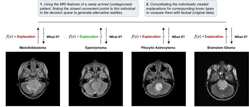
Figure 1: The figure illustrates a clinical scenario that demonstrates the practical application of counterfactuals and how they can be utilized in practice. The data used includes the features extracted from provided brain MRIs, not the images themselves.

2 Material & Methods

2.1 Ethics Statement and Patient Characteristics

This prospective study (Ref: 632 QÐ-NÐ2 dated 12 May 2019) was carried out in both Radiology and Neurosurgery departments, and was approved by the Institutional Review Board in accordance with the 1964 Helsinki declaration. Written informed consent was obtained from authorized guardians of patients prior to the MRI procedure. Our study comprised a cohort of 112 pediatric patients diagnosed with posterior fossa tumors, including 42 with MB, 25 with PA, 34 with BG, and 11 with EP. All BG patients were confirmed based on full agreement between neuroradiologists and neurosurgeons, whereas the remaining MB, PA, and EP patients underwent either surgery or biopsy for histopathological confirmation.

2.2 Data Acquisition and Assessment of MRI Features

For all patients, MRI exams including T1W, T2W, FLAIR, DWI (b values: 0 and 1000) with ADC, and contrast-enhanced T1W (CE-T1) sequences with macrocyclic gadolinium-based contrast enhancement (0.1 ml/kg Gadovist, Bayer, Germany, or 0.2 ml/kg Dotarem, Guerbet, France) were collected in the supine position using a 1.5 Tesla MRI scanner (Multiva, Philips, Best, the Netherlands).

The Medical Imaging Interaction Toolkit (German Cancer Research Center, Division of Medical Image Computing, Heidelberg, Germany) was utilized for measuring the region of interest (ROI) of posterior fossa tumors and normal-appearing parenchyma and and subsequently assessed the following MRI features: signal intensities (SIs) of T2, T1, FLAIR, T1CE, DWI, and ADC. Ratios between the posterior fossa tumor and parenchyma were calculated by dividing the SI of the tumor and the SI of the normal-appearing parenchyma based on T2, T1, FLAIR, T1CE, DWI, and ADC. Additionally, ADC values were quantified for both the posterior fossa tumor and parenchyma on the ADC map using the MR Diffusion tool available in Philips Intellispace Portal, version 11 (Philips, Best, The Netherlands). It is worth noting that, prior to analysis, bias field correction was applied to every image to correct for nonuniform grayscale intensities in the MRI caused by field inhomogeneities.

2.3 Standardization

Prior to conducting ML trainings, the dataset was subjected to a standardization process, using Python programming (version 3.9.13) with the Scikit-Learn library (version 1.0.2) module. This technique involved transforming the data to have a mean of zero and a standard deviation of one. To standardize all numerical attributes, the Scikit-Learn StandardScaler function was employed, which subtracted the mean and scaled the values to unit variance, ensuring the data was in a standardized format. To determine the standard score of a sample $x_{i}$ , the following formula is used:

$$z=\frac{x_{i}-\mu}{\sigma},$$ (1)

where, $\mu$ represents the mean of the training samples, and $\sigma$ represents their standard deviation.

2.4 Distance Calculation

Utilizing counterfactuals as classifiers, the notable discrepancy in MRI feature values between Tables 1 and 2 complicates distance calculations. We addressed this by omitting unchanged values (‘-’), rescaling the rest to a consistent scale, and then reintroducing them. The distances were then computed using the Euclidean metric on the counterfactual values of the current factual. Minimizing this distance aids in determining the tumor type by corresponding to the least dissimilarity (Table 3). The Euclidean distance is given by:

$$\mathrm{Distance}=\sqrt{\sum_{i=1}^{n}(x_{i}-y_{i})^{2}}$$ (2)

Here, $x_{i}$ and $y_{i}$ are values from the current and baseline rows, respectively. The formula sums the squared differences for each feature, then takes the square root. In this equation, $n$ signifies the feature count in the dataset.

2.5 Statistical Analysis

Using the $t$-test from the scipy library (version 1.10.1), we considered a two-tailed $p$-value of $<0.05$ as statistically significant. Our analysis comprised:

1. Assessing the statistical significance of changes in counterfactuals when transitioning the tumor type from $\mathcal{X}$ to $\mathcal{Y}$ (dependent $t$-test).

2. Comparing the similarity between counterfactuals transitioning from $\mathcal{X}$ to $\mathcal{Y}$ and the original patients with tumor type $\mathcal{Y}$ (Welch’s $t$-test).

For each transition from tumor type $\mathcal{X}$ to $\mathcal{Y}$, we generated five counterfactuals. In our $t$-test evaluations, these counterfactuals were examined in distinct manners. Due to generating a dataset larger than our original sample size, we could not maintain equal dimensions for the dependent analysis. To address this:

• For each counterfactual, we used the data of the corresponding factual patient as a baseline for testing.

• We subsequently tested the significance of the top five most changed feature variables.

For the independent analysis, all counterfactuals were evaluated using the real data of all patients, focusing on the three most altered features. Each feature was evaluated separately.

In summary, the primary distinction between our tests was their focus: one on patients, and the other on features.

2.6 Distribution Plotting

To generate individual kernel density estimation (KDE) plots for each feature, we utilized the kdeplot function from the Seaborn package (version 0.11.2). By specifying a hue parameter (e.g., Tumor Type), we were able to incorporate a meaningful association using this method. Consequently, we transformed the default marginal plot into a layered KDE plot. This approach tackles the challenge of reconstructing the density function $f$ using an independent and identically distributed (iid) sample $x_{1},x_{2},...,x_{n}$ from the respective probability distribution.

2.7 Machine Learning

To decrease overfitting and convergence issue of counterfactuals, especially for EP, we took less patients to implement the task: 25 patients from MB, PA and BG and 11 patients from EP. For testing, to ensure the reliability of our ML models, particularly with a small dataset, we conducted five runs using stratified random sampling based on tumor type with 55% train and 45% test patients.

Using nine ML models, including support vector machine (SVM), adaboost (ADA), logistic regression (LR), random forest classifier (RF), decision tree classifier (DT), gradient boosting classifier (GB), catboost classifier (CB), extreme gradient boosting classifier (XGB) and voting classifier (VOTING), we evaluated the models on the raw data with the outcomes prior to our counterfactual interpretations. CB and XGB were obtained from CatBoost version 1.1.1 and XGBoost version 1.5.1 libraries, respectively, while the other models were obtained from the Scikit-Learn library.

We assessed the performance of the models using precision, recall, and F1 score, which were calculated based on the counts of true positives (TP), true negatives (TN), false positives (FP), and false negatives (FN). In order to ensure an accurate interpretation of the ML results, we opted not to balance the labels. Instead, we employed macro precision, macro recall, and macro F1 score metrics, which take into account the contributions of all labels equally. This approach enabled us to observe the genuine impact of the varying label frequencies, EP in this case.

3 Counterfactual Explanations

Given the challenges associated with local approximations, it is worthwhile to explore prior research in the "explanation sciences" to identify potential alternative strategies for generating reliable and practical post-hoc interpretations that benefit the stakeholders affected by algorithmic decisions [1, 17]. To create explanations that are understandable and useful for both experts and non-experts, it is logical to investigate theoretical and empirical studies that shed light on how humans provide and receive explanations [8]. Over the past few decades, the fields of philosophy of science and epistemology have shown increasing interest in theories related to counterfactual causality and contrastive explanations [17, 18, 19, 20, 21].

In philosophy, counterfactuals serve not only to assess the relationship between a mental state and reality, but also to determine whether a mental state can be considered as knowledge. The problem of identifying knowledge with justified true belief is complicated by various counterexamples, such as Gettier cases (1963) [22]. However, some scholars proposed additional conditions to address these counterexamples. This literature highlighted two significant counterfactual conditions:

Sensitivity: If $\rho$ were false, $\mathcal{S}$ would not believe that $\rho$.

Safety: If $\mathcal{S}$ were to believe that $\rho$, $\rho$ would not be false.

Both of these conditions express the notion that $\mathcal{S}$’s beliefs must be formed in a manner that is sensitive to the truthfulness of $\rho$. The counterfactual semantics has influenced from this idea in various ways, including the establishment of their non-equivalence, clarification, and resolution of potential counterexamples [23].

This concept has sparked a fresh wave of counterfactual analyses that employ new methodologies. Hitchcock [24, 25] and Woodward [26], for instance, constructed counterfactual analyses of causation using Bayesian networks (also known as "causal models") and structural equations. The basic idea of the analysis can be summarized as follows: "$\mathcal{X}$ can be considered a cause of $\mathcal{Y}$ only if there exists a path from $\mathcal{X}$ to $\mathcal{Y}$, and changing the value of $\mathcal{X}$ alone results in a change in the value of $\mathcal{Y}$".

Ginsberg (1986) [27] initiated his discussion by outlining the potential significance of counterfactuals in artificial intelligence and summarizing the philosophical insights that have been drawn regarding them. Following this, Ginsberg provided a structured explanation of counterfactual implication and analyzed the challenges involved in executing it. Over time, numerous developments in the fields of artificial intelligence and cognitive science, including the Bayesian epistemology approach, have gone beyond what was previously envisioned by Ginsberg regarding the potential application of artificial intelligence and counterfactuals [7, 8, 28, 29, 30, 31]. Furthermore, Verma et al. [32] conducted a comprehensive review of the counterfactual literature, analyzing its utilization in over 350 research papers.

In recent times, there has been a growing interest in the concept of counterfactual explanations, which aim to provide alternative perturbations capable of changing the predictions made by a model. In simple terms, when given an input feature $x$ and the corresponding output produced by an ML model $f$, a counterfactual explanation involves modifying the input to generate a different output $y$ using the same algorithm. To further explain this concept, Wachter et al. [7] introduce the following formulation in their proposal:

$$c=\arg\min\limits_{c}\ell(f(c),y)+|x-c|$$ (3)

The initial component $\ell$ of the formulation encourages the counterfactual $c$ to deviate from the original prediction, aiming for a different outcome. Meanwhile, the second component ensures that the counterfactual remains in proximity to the original instance, thereby emphasizing the importance of maintaining similarity between the two.

3.1 Generating Counterfactual Explanations

Causality in counterfactuals is relevant for decision-making regarding an individual’s future [33, 34, 35, 36, 37, 38, 11, 39, 40]. In situations where a negative response is received, understanding how to improve results without resorting to major and unrealistic data alterations becomes important.

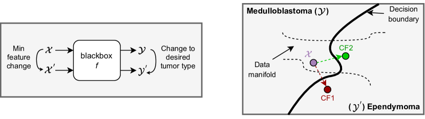
Figure 2: Generating counterfactual explanations on tumor types. The left illustrates feature manipulation using an ML model with a counterfactual approach. The right delves deeper into the process and counterfactual explanation concept, exemplified by two tumor types.

We argue that the use of counterfactual explanations effectively leverages the factual insights derived from MRI features. These features act as distinct markers, facilitating the differentiation between various tumors. Such a methodology shines particularly when traditional diagnostics find it challenging to distinguish between tumor types.

The data manifold concept, illustrated in Fig. 2, emphasizes the importance of proximity in counterfactual explanations. For counterfactuals to be credible, their features should resemble those of prior classifier observations and be realistic. Counterfactuals with features that diverge from training data or disrupt feature associations are impractical and outside established norms [41]. To ensure that counterfactuals are realistic and align with the training data, we employ constraint-based approaches in our algorithms. For instance, changing parameters such as "age" and "gender" would be highly unreasonable. Therefore, in most scenarios, these parameters are specified in the model to prevent counterfactuals from deviating from reality. Similarly, in our case, while parenchyma features were included during training, they remain invariant during counterfactual generation to preserve tissue characteristic references.

The DiCE library [42] offers a framework for counterfactual generation, viewing it as an optimization task akin to adversarial example discovery. Crucially, the modifications must be diverse, feasible, and implementable. The optimization formula used is:

$$C(x)=\arg\min\limits_{c_{1},...,c_{k}}\frac{1}{k}\sum_{i=1}^{k}\ell(f(c_{i}),y)+\frac{\lambda_{1}}{k}\sum_{i=1}^{k}\mathrm{dist}(c_{i},x)-\lambda_{2}\,\mathrm{dpp\_diversity}(c_{1},...,c_{k}),$$ (4)

with hinge loss as:

$$\ell=\max(0,1-z*\mathrm{logit}(f(c))),$$ (5)

where $z$ takes values based on $y$ and logit($f(c)$) represents unscaled ML output. Diversity is expressed as:

$$\mathrm{dpp\_diversity}=\mathrm{det(K)},$$ (6)

where $\mathrm{K}_{i,j}=\frac{1}{1+\mathrm{dist}(c_{i},c_{j})}$, and the distance between counterfactuals is measured.

4 Results

4.1 What if the counterfactual explanations graciously provide us with additional insights into classification?

Using DiCE’s multi-class training capability, we have established a framework that simultaneously trains for four distinct tumor types. This framework employs counterfactual explanations, serving as classifiers, to determine tumor types based on numeric MRI data. By utilizing all four tumor types, we essentially construct a decision space of reality with our existing patients. As the new patient is guided through this space, attempting to transform into each disease sequentially, the degree of self-modification required for each specific tumor condition will vary. As the required changes decrease, it can be inferred that the patient is closer to that particular tumor type since they necessitate fewer modifications. Similarly, understanding the level of dissimilarity and the contributing features to this dissimilarity has been explored as a critical approach in determining the tumor type. Among the models evaluated, the LR model demonstrated superior efficacy, especially in generating counterfactuals, thus affirming its selection for our research.

Figure 1 and Table 1 present a scenario involving a patient diagnosed via MRI with an indeterminate tumor type. Using the MRI data, we generate "what-if" scenarios for each tumor type. These scenarios, based on feature distances, help determine the tumor type the patient’s data aligns with.

Factual ($x$)
Tumor Type	T2_T	T2_R	FLAIR_T	FLAIR_R	DWI_T	DWI_R	ADC_T	ADC_R	T1_T	T1_R	T1CE_T	T1CE_R
unknown (EP)	1286	1.529	1311	1.341	1175	1.088	1.009	1.771	473	0.84	892	1.595

Counterfactual ($x_{cf}$)
Tumor Type	T2_T	T2_R	FLAIR_T	FLAIR_R	DWI_T	DWI_R	ADC_T	ADC_R	T1_T	T1_R	T1CE_T	T1CE_R
MB	-	-	648	-	-	-	-	-	-	-	1309.5	-
EP	1423.2	-	-	-	-	-	-	-	-	-	-	-
PA	2290.2	-	-	-	-	-	2	-	-	-	1492.5	-
BG	-	-	-	-	544.23	-	2	-	-	-	-	0.781

Table 1: This table presents the results of our proposed method utilizing counterfactuals (Fig. 1).

Table 1 details an unknown patient classified as EP. For the MB counterfactual, changes in FLAIR_Tumor and T1CE_Tumor result in distances of -663 and 417.5, respectively. For EP, T2_Tumor changes, resulting in a distance of 137.2. In the PA group, changes are observed in T2_Tumor (from 1286 to 2290.2), ADC_Tumor (from 1.009 to 2), and T1CE_Tumor (from 892 to 1492.5). For the BG group, DWI_Tumor changes from 1175 to 544.23, ADC_Tumor from 1.009 to 2, and T1CE_Ratio from 1.595 to 0.781.

Table 2 introduces more potential cases. For the MB counterfactual, FLAIR_Ratio changes from 1.141 to 0.742. For EP, changes are observed in FLAIR_Tumor (from 1107 to 2493) and ADC_Ratio (from 0.87 to 2.316). In PA, T2_Ratio changes from 1.638 to 2.61 and ADC_Ratio from 0.87 to 2.892. For BG, changes are seen in ADC_Tumor (from 0.54 to 2.05) and ADC_Ratio (from 0.87 to 2.917).

For PA in Table 2, changes in MB are from 2.297 to 0.97 in T2_Ratio, 1.143 to 0.608 in FLAIR_Ratio, 1.879 to 0.4 in ADC_Tumor, and 0.57 to 0.535 in T1_Ratio. For EP, T2_Tumor changes from 1778 to 913.6, T2_Ratio from 2.297 to 0.968, DWI_Tumor from 809 to 402.32, DWI_Ratio from 0.805 to 0.476, and ADC_Tumor from 1.879 to 0.4. In BG, T2_Ratio changes from 2.297 to 1.072 and T1CE_Ratio from 1.125 to 0.768.

For BG in Table 2, changes are observed in T2_Tumor (from 1709 to 860.3), T2_Ratio (from 1.724 to 0.908), FLAIR_Tumor (from 1150 to 2019), and ADC_Tumor (from 1.59 to 0.34) for the EP counterfactual. For PA, ADC_Tumor changes from 1.59 to 1.56 and T1CE_Tumor from 326 to 1234. For BG, FLAIR_Ratio changes from 1.189 to 0.752.

In Tables 1, 2, and 3, T represents Tumor and R represents Ratio (Tumor/Parenchyma). The symbol (-) indicates no modification. In Table 1, the patient, with the lowest feature distance to EP, is predicted as EP.

Table 3 displays the same samples as Tables 1 and 2, but with standardized features. Distances are provided for each patient’s tumor type and their respective counterfactuals. The data represented by (-) matches original values. The distance metric adjusts the distance magnitude between them.

	Tumor Type	T2_T	T2_R	FLAIR_T	FLAIR_R	DWI_T	DWI_R	ADC_T	ADC_R	T1_T	T1_R	T1CE_T	T1CE_R
Factual ($x$)	unknown (MB)	1534	1.638	1107	1.141	1883	1.614	0.54	0.87	513	0.842	818	1.327
Counterfactual ($x_{cf}$)	MB	-	-	-	0.742	-	-	-	-	-	-	-	-
Counterfactual ($x_{cf}$)	EP	-	-	2493	-	-	-	-	2.316	-	-	-	-
Counterfactual ($x_{cf}$)	PA	-	2.61	-	-	-	-	-	2.892	-	-	-	-
Counterfactual ($x_{cf}$)	BG	-	-	-	-	-	-	2.05	2.917	-	-	-	-
Factual ($x$)	unknown (PA)	1778	2.297	1085	1.143	809	0.805	1.879	2.685	439	0.57	747	1.125
Counterfactual ($x_{cf}$)	MB	-	0.967	-	0.608	-	-	0.4	-	-	0.535	-	-
Counterfactual ($x_{cf}$)	EP	913.6	0.968	-	-	402.32	0.476	0.4	-	-	-	-	-
Counterfactual ($x_{cf}$)	PA	-	-	-	-	-	1.025	-	-	-	-	-	-
Counterfactual ($x_{cf}$)	BG	-	1.072	-	-	-	-	-	-	-	-	-	0.768
Factual ($x$)	unknown (BG)	1709	1.724	1150	1.189	1112	0.674	1.59	2.148	373	0.643	326	0.652
Counterfactual ($x_{cf}$)	MB	1000.9	-	974	0.669	-	-	0.5	0.677	1424	0.573	479.9	0.76
Counterfactual ($x_{cf}$)	EP	860.3	0.908	2019	-	-	-	0.34	-	-	-	-	-
Counterfactual ($x_{cf}$)	PA	-	-	-	-	-	-	1.56	-	-	-	1234	-
Counterfactual ($x_{cf}$)	BG	-	-	-	0.752	-	-	-	-	-	-	-	-

Table 2: The table presents additional counterfactual cases generated for different newly arriving patients. The Tumor and Ratio features are not on the same scale for direct comparison due to their mathematical dependency.

	Tumor Type	T2_T	T2_R	FLAIR_T	FLAIR_R	DWI_T	DWI_R	ADC_T	ADC_R	T1_T	T1_R	T1CE_T	T1CE_R	Distance
Factual ($x$)	unknown (MB)	0	-0.5	-0.5	0.5	0	0	-0.5	-1.191	0	0	0	0	-
Counterfactual ($x_{cf}$)	MB	-	-	-	-2	-	-	-	-	-	-	-	-	2.5
Counterfactual ($x_{cf}$)	EP	-	-	2	-	-	-	-	0.370	-	-	-	-	2.948
Counterfactual ($x_{cf}$)	PA	-	2	-	-	-	-	-	0.993	-	-	-	-	3.319
Counterfactual ($x_{cf}$)	BG	-	-	-	-	-	-	2	1.020	-	-	-	-	3.337
Factual ($x$)	unknown (EP)	-0.583	0	0.5	0	0.5	0	-0.816	0	0	0	-0.795	0.5	-
Counterfactual ($x_{cf}$)	MB	-	-	-2	-	-	-	-	-	-	-	0.836	-	2.985
Counterfactual ($x_{cf}$)	EP	-0.233	-	-	-	-	-	-	-	-	-	-	-	0.350
Counterfactual ($x_{cf}$)	PA	1.982	-	-	-	-	-	1.225	-	-	-	1.550	-	4.031
Counterfactual ($x_{cf}$)	BG	-	-	-	-	-2	-	1.225	-	-	-	-	-2	4.082
Factual ($x$)	unknown (PA)	0.5	1.223	0	0.5	0.5	0.124	0.816	0	0	0.5	0	0.5	-
Counterfactual ($x_{cf}$)	MB	-	-0.871	-	-2	-	-	-1.225	-	-	-2	-	-	4.588
Counterfactual ($x_{cf}$)	EP	-2	-0.869	-	-	-2	-1.749	-1.225	-	-	-	-	-	4.955
Counterfactual ($x_{cf}$)	PA	-	-	-	-	-	1.377	-	-	-	-	-	-	1.252
Counterfactual ($x_{cf}$)	BG	-	-0.705	-	-	-	-	-	-	-	-	-	-2	3.157
Factual ($x$)	unknown (BG)	0.811	0.5	-0.373	0.811	0	0	0.831	0.5	-0.5	0.5	-0.602	-0.5	-
Counterfactual ($x_{cf}$)	MB	-1.033	-	-0.847	-1.393	-	-	-1.079	-2	2	-2	-0.166	2	6.109
Counterfactual ($x_{cf}$)	EP	-1.400	-2	1.966	-	-	-	-1.360	-	-	-	-	-	4.627
Counterfactual ($x_{cf}$)	PA	-	-	-	-	-	-	0.778	-	-	-	1.971	-	2.574
Counterfactual ($x_{cf}$)	BG	-	-	-	-1.041	-	-	-	-	-	-	-	-	1.853

Table 3: Distance results for counterfactuals generated on feature-wise scaled data for four distinct newly arriving patients with varying tumor types.

4.2 Revealing Key MRI Features through Counterfactual Explanations

As discussed in Section 3.1, counterfactual explanations can provide insights into feature importance. These explanations allow us to understand the reasoning behind ML model decisions and offer valuable options for restriction. In clinical settings, visible changes in features through counterfactual explanations can be more relevant and meaningful for real-world evaluations and applications.

Considering that we generated five counterfactuals for each patient, we obtained 125 explanations for MB, PA, and BG, and 55 explanations for EP. Table 4 illustrates our reporting method for counterfactual analysis results for a case scenario (MB to EP). The patient count, the total number of generated counterfactual explanations for them, and the statistical information regarding the frequency of changes observed on which features in these counterfactuals to identify the top 3 influential features are shown. For instance, "FLAIR_Tumor 71 changes" signifies that out of 125 counterfactuals, 71 of them involved a modification from MB to EP. Therefore, FLAIR_Tumor creates such a distinction between these two tumors that the model considers altering this feature significantly influential in shifting the decision from one side to the other in the decision space. The greater the repetition of this occurrence, indicated by the magnitude of "changes," the more pronounced the outcome suggesting that even in random selections, optimization is achieved for that particular feature, significantly impacting the decision.

Number of patients: 25
Number of generated counterfactuals: 125
FLAIR_Tumor	71 changes		T1_Ratio	6 changes
ADC_Tumor	33 changes		T1CE_Tumor	6 changes
ADC_Ratio	29 changes		T2_Tumor	3 changes
DWI_Ratio	18 changes		T2_Parenchyma	0 changes
FLAIR_Ratio	17 changes		FLAIR_Parenchyma	0 changes
DWI_Tumor	12 changes		DWI_Parenchyma	0 changes
T1_Tumor	10 changes		ADC_Parenchyma	0 changes
T1CE_Ratio	7 changes		T1_Parenchyma	0 changes
T2_Ratio	6 changes		T1CE_Parenchyma	0 changes

Table 4: This example analysis presents the variations in characteristics observed during the generation of counterfactual instances for the transition from MB to EP.

Table 5 presents the findings from each tumor pair to identify feature differences between different tumor types. The observed changes in features align with expected outcomes from clinical studies. MB and EP tumors are distinguished by FLAIR and ADC features. MB and PA typically exhibit differences in T2 and ADC. MB and BG, on the other hand, show variations primarily in ADC, T2, and T1CE. In the case of EP and PA, T2 exhibits the most significant changes, while variations in ADC and T1CE are also observed. The most distinguishing features between EP and BG are T1CE_Ratio and ADC_Tumor. As for PA and BG, the T2_Ratio feature has been identified as a crucial factor in creating differentiation. Additionally, significant variations in T1CE features are frequently observed, further contributing to the dissimilarity between these tumor types.

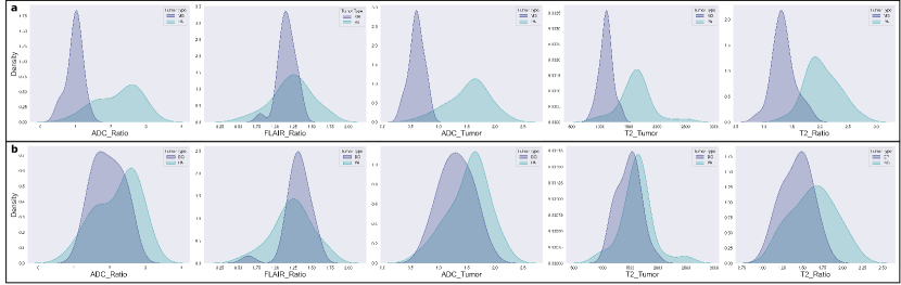
Figure 3: Original data distributions for MB - PA and BG - PA, focusing on specific features.

The results presented in Table 5, along with the visualization in Fig. 3, provide insights into the PA example as follows: When considering the scenarios of MB to PA or PA to MB, it is generally observed that similar distributions dominate. The distinctiveness of the distributions between MB and PA becomes evident when examining the top 5 features that exhibit the most variation, as shown in Fig. 3 and discussed in our previous study [43]. Furthermore, when examining nearly identical distributions between BG and PA, a lack of discernibility is found. This is further supported by the absence of these features among the important features for BG to PA or PA to BG, as demonstrated in Table 5. These findings indicate that the algorithm effectively operates in accordance with our expectation during counterfactual generation, which involves altering the most distinct features to achieve maximum impact with minimal modification. Notably, T1CE features and T2_Ratio are identified as the most distinctive features between PA and BG, as shown in Fig. 5 of [43].

MB to EP			MB to PA			MB to BG			EP to MB			EP to PA			EP to BG
Feature	Change		Feature	Change		Feature	Change		Feature	Change		Feature	Change		Feature	Change
FLAIR_Tumor	71		T2_Ratio	87		T2_Tumor	64		T1CE_Tumor	18		T2_Tumor	34		ADC_Tumor	22
ADC_Tumor	33		T2_Tumor	55		ADC_Tumor	52		FLAIR_Ratio	16		T2_Ratio	26		DWI_Ratio	16
ADC_Ratio	29		ADC_Tumor	43		T1CE_Ratio	43		FLAIR_Tumor	13		ADC_Tumor	19		T1CE_Ratio	15
PA to MB			PA to EP			PA to BG			BG to MB			BG to EP			BG to PA
Feature	Change		Feature	Change		Feature	Change		Feature	Change		Feature	Change		Feature	Change
ADC_Ratio	91		T2_Ratio	95		T2_Ratio	95		FLAIR_Ratio	85		T1CE_Ratio	90		T1CE_Ratio	53
FLAIR_Ratio	88		T2_Tumor	81		T1CE_Tumor	66		ADC_Tumor	71		T1_Tumor	50		T1CE_Tumor	48
ADC_Tumor	76		T1CE_Tumor	45		T1CE_Ratio	54		ADC_Ratio	71		DWI_Ratio	48		T2_Ratio	32

Table 5: The three most important features for each changing reality case.

4.3 Statistical Analysis of Generated Counterfactuals

During the construction of the counterfactual tumor $y$ from the original tumor $x$, we conducted a dependent test to assess the statistical difference between $x$ and $y$, as explained in Section 2.5. Apart from the PA to MB transition (e.g., $p$=0.04763, $p$=0.0307), no significant differences were observed in other tumor transitions. This result can be attributed to both the fundamental optimization principle of minimizing changes during counterfactual generation and the distribution distances shown in Fig. 3. Specifically, Fig. 3a demonstrates a distinct separation in the distributions during the PA to MB transition, requiring a significantly larger change for transformation.

MRI Feature	Original	Generated	T-Statistic	P-Value
DWI_Tumor	MB	MB to MB	-0.0605	0.9521
T1CE_Ratio	MB	MB to MB	-0.3643	0.7177
T1_Ratio	MB	MB to MB	-0.0282	0.9776
T1CE_Tumor	MB	EP to MB	-2.4975	0.0156
FLAIR_Ratio	MB	EP to MB	0.4532	0.6524
FLAIR_Tumor	MB	EP to MB	0.7917	0.4331
ADC_Ratio	MB	PA to MB	-0.4017	0.6887
FLAIR_Ratio	MB	PA to MB	11.5615	<0.0001
ADC_Tumor	MB	PA to MB	-4.3706	<0.0001
FLAIR_Ratio	MB	BG to MB	6.7026	<0.0001
ADC_Tumor	MB	BG to MB	-5.2062	<0.0001
ADC_Ratio	MB	BG to MB	-2.7487	0.0071

(a) Difference between original MB and generated MBs.

MRI Feature	Original	Generated	T-Statistic	P-Value
FLAIR_Tumor	EP	MB to EP	-3.2397	0.0061
ADC_Tumor	EP	MB to EP	-2.0273	0.0495
ADC_Ratio	EP	MB to EP	-0.6434	0.5266
FLAIR_Tumor	EP	EP to EP	-1.0603	0.3018
ADC_Tumor	EP	EP to EP	-1.4653	0.1519
DWI_Ratio	EP	EP to EP	-0.4937	0.6278
T2_Ratio	EP	PA to EP	2.956	0.007
T2_Tumor	EP	PA to EP	0.3621	0.72
T1CE_Tumor	EP	PA to EP	-1.1672	0.262
T1CE_Ratio	EP	BG to EP	-2.1967	0.0428
T1_Tumor	EP	BG to EP	-5.9549	<0.0001
DWI_Ratio	EP	BG to EP	0.0059	0.9954

(b) Difference between original EP and generated EPs.

MRI Feature	Original	Generated	T-Statistic	P-Value
T2_Ratio	PA	MB to PA	-2.0667	0.0430
T2_Tumor	PA	MB to PA	-0.1256	0.9004
ADC_Tumor	PA	MB to PA	4.4019	<0.0001
T2_Tumor	PA	EP to PA	-1.3925	0.1694
T2_Ratio	PA	EP to PA	1.6279	0.1091
ADC_Tumor	PA	EP to PA	3.6692	0.0005
ADC_Tumor	PA	PA to PA	0.2781	0.7822
T1_Ratio	PA	PA to PA	-0.8599	0.3948
FLAIR_Tumor	PA	PA to PA	-1.2497	0.2176
T1CE_Ratio	PA	BG to PA	1.711	0.0944
T1CE_Tumor	PA	BG to PA	1.7524	0.0862
T2_Ratio	PA	BG to PA	2.2029	0.0326

(c) Difference between original PA and generated PAs.

MRI Feature	Original	Generated	T-Statistic	P-Value
T2_Tumor	BG	MB to BG	-2.4723	0.0149
ADC_Tumor	BG	MB to BG	5.6539	<0.0001
T1CE_Ratio	BG	MB to BG	-6.6115	<0.0001
ADC_Tumor	BG	EP to BG	2.8215	0.0066
DWI_Ratio	BG	EP to BG	0.806	0.4236
T1CE_Ratio	BG	EP to BG	-4.4199	<0.0001
T2_Ratio	BG	PA to BG	6.78	<0.0001
T1CE_Tumor	BG	PA to BG	-5.3162	<0.0001
T1CE_Ratio	BG	PA to BG	-6.9185	<0.0001
ADC_Tumor	BG	BG to BG	-0.3252	0.7467
DWI_Tumor	BG	BG to BG	-0.8181	0.4176
DWI_Ratio	BG	BG to BG	-0.7461	0.4599

(d) Difference between original BG and generated BGs.

Table 6: The results of hypothesis tests comparing the original data with the generated data.

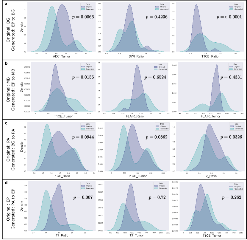
Figure 4: The distributions of the original data and the generated data.

Table 6 presents the statistical similarity obtained when each tumor is transformed to represent the "what if?" scenario of other tumors. In other words, when we transform tumor $x$ to tumor $x^{\prime}$=$y$, we know that $x^{\prime}$ is still dependent on x. Therefore, we measure how similar $x^{\prime}$ is to the original distribution of $y$ on the feature where $x$ undergoes the most significant change. A high $p$-value indicates that we do not reject the difference, implying that the counterfactual explanations we generate sufficiently resemble the original distribution for that particular feature.

As expected, when attempting self-transformation on each tumor type, the obtained $p$-values were notably high. Evaluating at a significance level of 0.05, several features closely aligned with the actual feature distribution of the patients, making them indistinguishable from the ground truth. The following features exhibited this characteristic: FLAIR_Ratio and FLAIR_Tumor in the case of transforming EP to MB, ADC_Ratio when transforming PA to MB, ADC_Ratio during the transformation from MB to EP, T2_Tumor and T1CE_Tumor in the context of PA to EP transformation, DWI_Ratio when transforming BG to EP, T2_Tumor for MB to PA transformation, T2_Tumor and T2_Ratio in the case of EP to PA transformation, T1CE_Ratio and T1CE_Tumor during BG to PA transformation, and DWI_Ratio when transforming EP to BG. Fig. 4 presents some of these cases along with their KDE distributions.

4.4 Pushing the Boundaries of Data Augmentation through Alternative Realities

During the construction of counterfactuals, we employed downsampling for MB and BG to align with the number of PA patients (25) during training, considering it appropriate. EP had a count of 11, and we did not increase it. The baseline results for this scenario can be observed in Table 7. For evaluation, the train-test splitting was conducted with a ratio of 45% for the baseline dataset, 35% for EP augmentation, and 25% for EP-PA-BG augmentation.

	Precision	Recall	F1 Score
Baseline	73.15 ± 9.48	72.20 ± 4.78	71.28 ± 5.62
A	84.83 ± 4.95	83.75 ± 3.72	83.34 ± 3.65
B	86.31 ± 4.57	84.64 ± 4.69	84.85 ± 4.72
C	73.58	72.73	72.04

Table 7: The impact of data augmentation using counterfactuals on classification scores is presented in the table. (A) For the first augmentation scenario, only EP counterfactuals are added, resulting in a dataset with 25 samples each for MB, EP, PA, and BG. (B) In the second augmentation scenario, counterfactuals for EP, PA, and BG are added to balance the number of samples with original count of MB. Assuming all counterfactual examples represent real data, this scenario results from a dataset comprising 42 samples each for MB, EP, PA, and BG. (C) The third scenario involves moving all real samples to the test set, with 11 patients in each category. Consequently, no factual EP samples are left in the training set, and the model is trained accordingly. In all cases, LR consistently yields the best results, and all the reported results in the table are from the LR classifier.

To address the data imbalance, we examined the inclusion of generated counterfactuals for data augmentation. For example, by equalizing EP with the other tumor types and incorporating 14 different generated counterfactuals alongside the originals, we excluded EP-to-EP instances. Opting for transitions from various tumor types to maximize variance and generalizability, we achieved an improvement of up to 12.06% as shown in Table 7, case A.

To incorporate the previously set aside MB and BG data, we aligned all tumor types, except themselves, with counterfactuals generated from different tumor types. BG, PA, and EP were included with MB, and all were evaluated as a group of 42 patients, which was the maximum patient count for one tumor type. When considering the counterfactuals as actual patients, the outcomes align with the results presented in Table 7, case B.

Furthermore, in the case examined in Table 7, case C, 11 patients were included from each tumor type in the test set, resulting in no actual EP patients in the training set. Consequently, during training, we had 31 real samples for MB, 0 real and 31 counterfactual samples for EP, 14 real and 17 counterfactual samples for PA, and 23 real and 8 counterfactual samples for BG. Notably, when evaluating on real samples, the results were intriguing. Despite the absence of real EP patients in the training data, the model successfully identified 5 out of the 11 patients, leading to an overall baseline score that was, on average, 0.76% higher.

5 Discussion

Spatial heterogeneity in pediatric brain tumors, especially from the posterior fossa, complicates accurate differentiation [44, 45, 46, 47, 48, 49, 50, 51, 52]. Accurate diagnoses are essential since each tumor requires specific treatments impacting patient outcomes. While AI advancements in medical imaging are promising, their black-box nature hinders clinical adoption. Our study introduces a novel approach, leveraging counterfactual explanations to interpret MRI features, aiming to provide clinicians an intuitive tool. This research pioneers feature-based counterfactual investigations in pediatric brain tumors.

The medical literature highlights that individualized care is crucial, aligning with personalized healthcare [53, 54, 55, 56]. The ability to generate hypothetical scenarios for a patient based on MRI features offers a significant advantage in medical diagnosis. By creating what-if scenarios, radiologists are equipped with additional intuitive data, enhancing their decision-making ability. This approach could potentially mitigate the need for invasive procedures and provide a clearer perspective on the tumor’s nature based on MRI data alone. Our method produces tailored explanations for each patient, drawing from past cases, facilitating understanding of tumor differentiation based on MRI data.

The concept of counterfactuals, which has been debated in philosophy and psychology for decades, has found its place in the field of artificial intelligence under various names. Though the idea has historical roots, its comprehensive implementation in AI is a more recent phenomenon. Like many preceding studies, we have adapted this concept for the clinical domain, providing valuable insights for clinicians. Furthermore, our work enriches the literature on medical counterfactuals by offering a unique perspective tailored to specific tasks. Through counterfactuals, we demonstrate alternative possibilities within the decision space and elucidate the rationales behind specific decisions pertaining to pediatric patients.

To the best of our knowledge, no prior studies have addressed counterfactuals regarding posterior fossa tumors. We filled this gap and subjected results to statistical tests, presented in Section 4.3. We explored the utility of counterfactuals both as post-classifiers and indicators of significant MRI features. The LR model was the most effective, hence we used it for counterfactual generation.

We developed a framework aimed at enhancing the utility of counterfactuals beyond what DiCE offers for our case. While challenges like the inability to find optimal counterfactual explanations underscore the need for DiCE updates, there are alternative solutions. Dutta et al. [57] and Maragno et al. [58] propose alternative counterfactual algorithms to potentially overcome these challenges. Furthermore, Guidotti’s review [59] presents an extensive list of counterfactual algorithms. If faced with a sizable patient pool, considering a subsample and substituting excluded patients can aid in statistical testing. These alternate methods could optimize within a more favorable timeframe than DiCE.

Our approach, which utilizes counterfactual explanations in a classifier-like manner, eliminates the need to separate different test sets. Consequently, the performance of our machine learning models significantly exceeds the baseline scores, with only a few patients excluded from the decision space to simulate the scenario of newly arriving patients. In this scenario, all training samples serve as test patients as we explore the decision space. To accomplish this, DiCE provides valuable information about misclassified samples, allowing us to exclude the associated counterfactuals from the statistical analysis through post-processing.

Fig. 1 and Table 1 depict a hypothetical scenario involving a patient with an initially unknown EP tumor. The radiologist examining the MR images was uncertain about whether the tumor was of the MB or EP type. A key challenge in such cases is the lack of additional information, which often necessitates invasive procedures like brain surgery and tissue sampling for histopathological analysis to obtain a definitive diagnosis. To overcome this issue, we generate alternative scenarios based solely on the MRI features. These scenarios provide additional quantitative information to the radiologist, enabling them to assess the response based on the individual’s biological characteristics.

Moreover, Table 2 presents examples of other potential tumor cases, while Table 3 demonstrates the efficacy of our approach in identifying patients with diverse tumor types that were previously unidentified and not encompassed within the decision space. While ML models can also accomplish this task, our method offers an additional advantage by preserving information regarding tissue characteristics, which in turn reveal similarities or differences among tumors. Additionally, our approach calculates distances to other tumors by transforming the features into a uniform distribution through standard scaling, providing valuable insights about the proximity. This valuable information aids in our comprehension of the differentiation among tumors in the dataset.

Table 4 presents the total count of modifications made to susceptible features, with the exception of the parenchymas that serves as reference points, when generating samples for different patients. The statistical report enables a human verification of the optimization process, wherein minimal changes are implemented to achieve the desired outcome. It also confirms that the features exhibiting the highest variations during the generation of alternative realities are those with the most distinct distributions between two tumors. To elucidate the analysis of their distributions, we present Fig. 3 as a visual representation. Table 5 presents the top three most variable features extracted from the reports obtained for all tumor matches in Table 4. This provides a more concise overview of all the cases.

Table 6 exhibits a statistical analysis demonstrating the high degree of similarity between the generated data and reality across different data spaces, specifically focusing on the most frequently selected features. A high $p$-value indicates that the generated samples cannot be well distinguished, implying the effectiveness of the independent transformation process, which produces significant alternative realities separate from the original space. Fig. 4 illustrates an example of some transformations from Table 6, displaying their corresponding $p$-values, as well as the kernel density estimation of the generated data in comparison to the original data.

Our generated counterfactuals offer potential advantages for data augmentation. Traditional methods, like SMOTE [16], sometimes fall short in real-world alignment and interpretability. We suggest counterfactuals as a viable alternative, particularly when data is limited. As shown in Fig. 7, while case C cannot be benchmarked directly due to added test patients, the inclusion of more real samples enhances outcomes. This improvement aligns with findings in [43]. However, challenges arise when certain EP patients, which complicate differentiation, are considered. Despite these challenges, the ability to make accurate predictions for many patients without actual EP training data highlights the promise of our approach and suggests directions for future research.

Counterfactual explanations can also address model bias in medical diagnoses [60, 61]. Ensuring fairness and transparency in decision-making processes is vital, suggesting the value of counterfactuals in this direction.

There are recognized challenges in applying the DiCE method to diverse datasets, sometimes resulting in extended optimization times and difficulties achieving convergence. Addressing these challenges will be an essential step forward. Exploring alternative methodologies and delving deeper into the vast landscape of counterfactual algorithms might also be beneficial. Future research should focus on expanding the dataset’s scope and size to ensure a wider applicability. This will capture a broader range of pediatric posterior fossa tumors scenarios encountered in clinical practice. To further advance the field, it is recommended to incorporate additional advanced MRI protocols, enriching our understanding and diagnostic capabilities regarding pediatric posterior fossa tumors.

6 Conclusion

In conclusion, this paper introduces a novel application of interpretability in medical research, with a focus on pediatric posterior fossa brain tumors as a case study. By leveraging counterfactual explanations, the study provides personalized and context-specific insights, validates predicted outcomes, and illuminates the variations in predictions under different scenarios.

The proposed approach shows great promise in enhancing the interpretability of MRI features for medical research studies. By bridging the gap between ML algorithms and clinical decision-making, it has the potential to facilitate the adoption of advanced computational techniques in medical practice. Clinicians can benefit from valuable insights gained from the generated counterfactual explanations, leading to improved decision-making processes and ultimately better patient outcomes. Notably, the counterfactual explanations generated in this study maintain statistical and clinical fidelity in many cases, underscoring their significance.

To fully realize the potential of this approach, further research and validation are essential. Integrating counterfactual explanations into existing clinical workflows and evaluating their performance in real-world scenarios will be critical to ensuring the reliability and practicality of this method. The continued development and refinement of utilizing counterfactual explanations in MRI-based diagnoses could revolutionize the medical field, benefiting both patients and healthcare providers. Therefore, future studies with larger datasets within the same domain or for different diseases could yield even more robust alternative realities constructed from MRI features. Overall, this study represents a significant step forward in moving beyond known reality and improving the application of ML in medical research and practice.

7 Declaration of competing interest

The authors declare that they have no known competing financial interests or personal relationships that could have appeared to influence the work reported in this paper.

8 Institutional Review Board Statement

After obtaining approval from the Institutional Review Board of Children Hospital of 02 with approval number [Ref: 632 QÐ-NÐ2 dated 12 May 2019], we conducted the study in both Radiology and Neurosurgery departments in accordance with the 1964 Helsinki declaration.

9 Funding

The authors received no financial support for the research, authorship, and/or publication of this article.

10 Data & Code Availability

The datasets generated and/or analyzed during the current study are not publicly available due to privacy concerns but are available from the Dr. Keserci upon reasonable request.

The source codes of the presented study can be accessed at: https://github.com/toygarr/counterfactual-explanations-for-medical-research

References

- [1] Brent Mittelstadt, Chris Russell, and Sandra Wachter. Explaining explanations in ai. In Proceedings of the conference on fairness, accountability, and transparency, pages 279–288, 2019.
- [2] Alfredo Vellido. The importance of interpretability and visualization in machine learning for applications in medicine and health care. Neural computing and applications, 32(24):18069–18083, 2020.
- [3] Michele Avanzo, Lise Wei, Joseph Stancanello, Martin Vallieres, Arvind Rao, Olivier Morin, Sarah A Mattonen, and Issam El Naqa. Machine and deep learning methods for radiomics. Medical physics, 47(5):e185–e202, 2020.
- [4] Giovanni Cinà, Tabea Röber, Rob Goedhart, and Ilker Birbil. Why we do need explainable ai for healthcare, 2022.
- [5] Marco Tulio Ribeiro, Sameer Singh, and Carlos Guestrin. " why should i trust you?" explaining the predictions of any classifier. In Proceedings of the 22nd ACM SIGKDD international conference on knowledge discovery and data mining, pages 1135–1144, 2016.
- [6] Scott M Lundberg and Su-In Lee. A unified approach to interpreting model predictions. Advances in neural information processing systems, 30, 2017.
- [7] Sandra Wachter, Brent Mittelstadt, and Chris Russell. Counterfactual explanations without opening the black box: Automated decisions and the gdpr. Harv. JL & Tech., 31:841, 2017.
- [8] Tim Miller. Explanation in artificial intelligence: Insights from the social sciences. Artificial intelligence, 267:1–38, 2019.
- [9] Nick Pawlowski, Daniel Coelho de Castro, and Ben Glocker. Deep structural causal models for tractable counterfactual inference. Advances in Neural Information Processing Systems, 33:857–869, 2020.
- [10] Pedro Sanchez, Antanas Kascenas, Xiao Liu, Alison Q O’Neil, and Sotirios A Tsaftaris. What is healthy? generative counterfactual diffusion for lesion localization. In MICCAI Workshop on Deep Generative Models, pages 34–44. Springer, 2022.
- [11] Zhendong Wang, Isak Samsten, and Panagiotis Papapetrou. Counterfactual explanations for survival prediction of cardiovascular icu patients. In Artificial Intelligence in Medicine: 19th International Conference on Artificial Intelligence in Medicine, AIME 2021, Virtual Event, June 15–18, 2021, Proceedings, pages 338–348. Springer, 2021.
- [12] William Todo, Merwann Selmani, Béatrice Laurent, and Jean-Michel Loubes. Counterfactual explanation for multivariate times series using a contrastive variational autoencoder. In ICASSP 2023-2023 IEEE International Conference on Acoustics, Speech and Signal Processing (ICASSP), pages 1–5. IEEE, 2023.
- [13] Supriya Nagesh, Nina Mishra, Yonatan Naamad, James M Rehg, Mehul A Shah, and Alexei Wagner. Explaining a machine learning decision to physicians via counterfactuals. In Conference on Health, Inference, and Learning, pages 556–577. PMLR, 2023.
- [14] Sebastien C Wong, Adam Gatt, Victor Stamatescu, and Mark D McDonnell. Understanding data augmentation for classification: when to warp? In 2016 international conference on digital image computing: techniques and applications (DICTA), pages 1–6. IEEE, 2016.
- [15] Hongyi Zhang, Moustapha Cisse, Yann N Dauphin, and David Lopez-Paz. mixup: Beyond empirical risk minimization. arXiv preprint arXiv:1710.09412, 2017.
- [16] Nitesh V Chawla, Kevin W Bowyer, Lawrence O Hall, and W Philip Kegelmeyer. Smote: synthetic minority over-sampling technique. Journal of artificial intelligence research, 16:321–357, 2002.
- [17] David-Hillel Ruben. Explaining explanation. Routledge, 2015.
- [18] David K. Lewis. Counterfactuals. Cambridge, MA, USA: Blackwell, 1973.
- [19] Boris Kment. Counterfactuals and explanation. Mind, 115(458):261–310, 2006.
- [20] Jim Woodward. Explanation, invariance, and intervention. Philosophy of Science, 64(S4):S26–S41, 1997.
- [21] James Woodward, Edward N Zalta, et al. Scientific explanation. The Stanford, 2017.
- [22] Edmund L. Gettier. Is justified true belief knowledge? Analysis, 23(6):121–123, 1963.
- [23] William Starr. Counterfactuals. In Edward N. Zalta and Uri Nodelman, editors, The Stanford Encyclopedia of Philosophy. Metaphysics Research Lab, Stanford University, Winter 2022 edition, 2022.
- [24] Christopher Hitchcock. The intransitivity of causation revealed in equations and graphs. The Journal of Philosophy, 98(6):273–299, 2001.
- [25] Christopher Hitchcock. Prevention, preemption, and the principle of sufficient reason. The Philosophical Review, 116(4):495–532, 2007.
- [26] James Woodward. Making things happen: A theory of causal explanation. Oxford university press, 2005.
- [27] Matthew L Ginsberg. Counterfactuals. Artificial intelligence, 30(1):35–79, 1986.
- [28] Peter Spirtes, Clark Glymour, and Richard Scheines. Discovery algorithms for causally sufficient structures. Causation, prediction, and search, pages 103–162, 1993.
- [29] Peter Spirtes, Clark Glymour, and Richard Scheines. Causation, prediction, and search. MIT press, 2000.
- [30] Thomas L Griffiths, Nick Chater, Charles Kemp, Amy Perfors, and Joshua B Tenenbaum. Probabilistic models of cognition: Exploring representations and inductive biases. Trends in cognitive sciences, 14(8):357–364, 2010.
- [31] Yu-Liang Chou, Catarina Moreira, Peter Bruza, Chun Ouyang, and Joaquim Jorge. Counterfactuals and causability in explainable artificial intelligence: Theory, algorithms, and applications. Information Fusion, 81:59–83, 2022.
- [32] Sahil Verma, Varich Boonsanong, Minh Hoang, Keegan E Hines, John P Dickerson, and Chirag Shah. Counterfactual explanations and algorithmic recourses for machine learning: A review. arXiv preprint arXiv:2010.10596, 2020.
- [33] Jonah E Rockoff, Brian A Jacob, Thomas J Kane, and Douglas O Staiger. Can you recognize an effective teacher when you recruit one? Education finance and Policy, 6(1):43–74, 2011.
- [34] Austin Waters and Risto Miikkulainen. Grade: Machine learning support for graduate admissions. Ai Magazine, 35(1):64–64, 2014.
- [35] Wuyang Dai, Theodora S Brisimi, William G Adams, Theofanie Mela, Venkatesh Saligrama, and Ioannis Ch Paschalidis. Prediction of hospitalization due to heart diseases by supervised learning methods. International journal of medical informatics, 84(3):189–197, 2015.
- [36] Monica Andini, Emanuele Ciani, Guido De Blasio, Alessio D’Ignazio, and Viola Salvestrini. Targeting policy-compliers with machine learning: an application to a tax rebate programme in italy. Bank of Italy Temi di Discussione (Working Paper) No, 1158, 2017.
- [37] Susan Athey. Beyond prediction: Using big data for policy problems. Science, 355(6324):483–485, 2017.
- [38] Linyi Yang, Eoin M Kenny, Tin Lok James Ng, Yi Yang, Barry Smyth, and Ruihai Dong. Generating plausible counterfactual explanations for deep transformers in financial text classification. arXiv preprint arXiv:2010.12512, 2020.
- [39] Ran Xu, Yue Yu, Chao Zhang, Mohammed K Ali, Joyce C Ho, and Carl Yang. Counterfactual and factual reasoning over hypergraphs for interpretable clinical predictions on ehr. In Machine Learning for Health, pages 259–278. PMLR, 2022.
- [40] Zhen Yang, Yongbin Liu, Chunping Ouyang, Lin Ren, and Wen Wen. Counterfactual can be strong in medical question and answering. Information Processing & Management, 60(4):103408, 2023.
- [41] Katherine Elizabeth Brown, Doug Talbert, and Steve Talbert. The uncertainty of counterfactuals in deep learning. In The International FLAIRS Conference Proceedings, volume 34, 2021.
- [42] Ramaravind K Mothilal, Amit Sharma, and Chenhao Tan. Explaining machine learning classifiers through diverse counterfactual explanations. In Proceedings of the 2020 conference on fairness, accountability, and transparency, pages 607–617, 2020.
- [43] Toygar Tanyel, Chandran Nadarajan, Nguyen Minh Duc, and Bilgin Keserci. Deciphering machine learning decisions to distinguish between posterior fossa tumor types using mri features: What do the data tell us? Cancers, 15(16), 2023.
- [44] Luciana Porto, Alina Jurcoane, Dirk Schwabe, and Elke Hattingen. Conventional magnetic resonance imaging in the differentiation between high and low-grade brain tumours in paediatric patients. European Journal of Paediatric Neurology, 18(1):25–29, 2014.
- [45] M Koob and N Girard. Cerebral tumors: specific features in children. Diagnostic and interventional imaging, 95(10):965–983, 2014.
- [46] Eleni Orphanidou-Vlachou, Nikolaos Vlachos, Nigel P Davies, Theodoros N Arvanitis, Richard G Grundy, and Andrew C Peet. Texture analysis of t1-and t2-weighted mr images and use of probabilistic neural network to discriminate posterior fossa tumours in children. NMR in Biomedicine, 27(6):632–639, 2014.
- [47] Yashar Moharamzad, Morteza Sanei Taheri, Farhad Niaghi, and Elham Shobeiri. Brainstem glioma: Prediction of histopathologic grade based on conventional mr imaging. The neuroradiology journal, 31(1):10–17, 2018.
- [48] Felice D’Arco, Faraan Khan, Kshitij Mankad, Mario Ganau, Pablo Caro-Dominguez, and Sotirios Bisdas. Differential diagnosis of posterior fossa tumours in children: new insights. Pediatric Radiology, 48:1955–1963, 2018.
- [49] Nguyen Minh Duc and Huynh Quang Huy. Magnetic resonance imaging features of common posterior fossa brain tumors in children: a preliminary vietnamese study. Open Access Macedonian Journal of Medical Sciences, 7(15):2413, 2019.
- [50] Nguyen Minh Duc, Huynh Quang Huy, Chandran Nadarajan, and Bilgin Keserci. The role of predictive model based on quantitative basic magnetic resonance imaging in differentiating medulloblastoma from ependymoma. Anticancer Research, 40(5):2975–2980, 2020.
- [51] Nihaal Reddy, David W Ellison, Bruno P Soares, Kathryn A Carson, Thierry AGM Huisman, and Zoltan Patay. Pediatric posterior fossa medulloblastoma: the role of diffusion imaging in identifying molecular groups. Journal of Neuroimaging, 30(4):503–511, 2020.
- [52] Dehua Chen, Shan Lin, Dejun She, Qi Chen, Zhen Xing, Yu Zhang, and Dairong Cao. Apparent diffusion coefficient in the differentiation of common pediatric brain tumors in the posterior fossa: Different region-of-interest selection methods for time efficiency, measurement reproducibility, and diagnostic utility. Journal of Computer Assisted Tomography, 47(2):291, 2023.
- [53] Nitesh V Chawla and Darcy A Davis. Bringing big data to personalized healthcare: a patient-centered framework. Journal of general internal medicine, 28:660–665, 2013.
- [54] Arash Shaban-Nejad, Martin Michalowski, and David L Buckeridge. Health intelligence: how artificial intelligence transforms population and personalized health. NPJ digital medicine, 1(1):53, 2018.
- [55] Ketan Paranjape, Michiel Schinkel, and Prabath Nanayakkara. Short keynote paper: Mainstreaming personalized healthcare–transforming healthcare through new era of artificial intelligence. IEEE journal of biomedical and health informatics, 24(7):1860–1863, 2020.
- [56] Kevin B Johnson, Wei-Qi Wei, Dilhan Weeraratne, Mark E Frisse, Karl Misulis, Kyu Rhee, Juan Zhao, and Jane L Snowdon. Precision medicine, ai, and the future of personalized health care. Clinical and translational science, 14(1):86–93, 2021.
- [57] Sanghamitra Dutta, Jason Long, Saumitra Mishra, Cecilia Tilli, and Daniele Magazzeni. Robust counterfactual explanations for tree-based ensembles. In International Conference on Machine Learning, pages 5742–5756. PMLR, 2022.
- [58] Donato Maragno, Jannis Kurtz, Tabea E. Röber, Rob Goedhart, Ş. Ilker Birbil, and Dick den Hertog. Finding regions of counterfactual explanations via robust optimization, 2023.
- [59] Riccardo Guidotti. Counterfactual explanations and how to find them: literature review and benchmarking. Data Mining and Knowledge Discovery, pages 1–55, 2022.
- [60] Agnieszka Mikołajczyk, Michał Grochowski, and Arkadiusz Kwasigroch. Towards explainable classifiers using the counterfactual approach: global explanations for discovering bias in data. Journal of Artificial Intelligence and Soft Computing Research, 11(1):51–67, 2021.
- [61] Zichong Wang, Yang Zhou, Meikang Qiu, Israat Haque, Laura Brown, Yi He, Jianwu Wang, David Lo, and Wenbin Zhang. Towards fair machine learning software: Understanding and addressing model bias through counterfactual thinking. arXiv preprint arXiv:2302.08018, 2023.