Strong convergence rates for a full discretization of stochastic wave equation with nonlinear damping

Abstract

The paper establishes the strong convergence rates of a spatio-temporal full discretization of the stochastic wave equation with nonlinear damping in dimension one and two. We discretize the SPDE by applying a spectral Galerkin method in space and a modified implicit exponential Euler scheme in time. The presence of the super-linearly growing damping in the underlying model brings challenges into the error analysis. To address these difficulties, we first achieve upper mean-square error bounds, and then obtain mean-square convergence rates of the considered numerical solution. This is done without requiring the moment bounds of the full approximations. The main result shows that, in dimension one, the scheme admits a convergence rate of order $\tfrac{1}{2}$ in space and order $1$ in time. In dimension two, the error analysis is more subtle and can be done at the expense of an order reduction due to an infinitesimal factor. Numerical experiments are performed and confirm our theoretical findings.

AMS subject classification: 60H35, 60H15, 65C30

Keywords: stochastic wave equation, nonlinear damping, strong approximation, spectral Galerkin method, modified exponential Euler scheme

1 Introduction

Hyperbolic stochastic partial differential equations (SPDEs) play an essential role in a range of real application areas, see below for examples. In the last decade, these SPDEs have attracted considerable attention from both a theoretical and a numerical point of view. One of the fundamental hyperbolic SPDE is the stochastic wave equation (SWE). Stochastic wave equations are used for instance to model the motion of a vibrating string [9] or the motion of a strand of DNA in a fluid [20]. A damping term is often included to the wave equation to model energy dissipation and amplitude reduction, see for instance the references [3, 13, 25, 23, 4] on stochastic wave equations with damping.

In the present work, we focus on the strong approximation of the solution to the following SWE with nonlinear damping in a domain $\mathcal{D}$:

$$\begin{split}\left\{\begin{array}[]{lll}\mathrm{d}u(t)=v(t)\,\mathrm{d}t,\\ \mathrm{d}v(t)=\left(\Delta u(t)+F(v(t))\right)\,\mathrm{d}t+\mathrm{d}W^{Q}(t),\quad t\in(0,T],\\ u(0)=u_{0},\,v(0)=v_{0},\end{array}\right.\end{split}$$ (1.1)

with homogeneous Dirichlet boundary conditions. Here, $\Delta$ denotes the Laplace operator and $\mathcal{D}\subset\mathbb{R}^{d}$, with $d\in\{1,2\}$, is a bounded domain with smooth boundary $\partial\mathcal{D}$. Precise assumptions on $F$, the noise $W^{Q}$ on a given probability space $(\Omega,\mathcal{F},\mathbb{P},\{\mathcal{F}_{t}\}_{t\geq 0})$ as well as the initial value $(u_{0},v_{0})$ are provided in the next section.

As opposed to the large amount of works on the numerical analysis of SPDEs of parabolic type, see for instance the books [31, 35] and references therein for the globally Lipschitz setting and [5, 6, 7, 10, 11, 17, 22, 24, 29, 34, 38, 45] for the non-globally Lipschitz setting, the literature on the numerical analysis of SPDEs of hyperbolic type is relatively scarce. The numerical analysis of SWEs without damping has been investigated by several authors, see for example [2, 12, 15, 16, 18, 30, 39, 43, 44, 46, 33, 19, 26, 14, 27]. For instance, in the work [2], the strong convergence rate of a fully discrete scheme for a stochastic wave equation driven by (a possibly cylindrical) $Q$-Wiener process is obtained together with an almost trace formula; Walsh in [43] used an adaptation of the leapfrog discretization to construct a fully discrete finite difference scheme which achieves a convergence order of $\tfrac{1}{2}$ in both time and space for an SPDE driven by space-time white noise; the authors of [46] presented strong approximations of higher order by using linear functionals of the noise process in the time-stepping schemes. For stochastic strongly damped wave equations, Qi and Wang in [37] investigated the regularity and strong approximations of a full discretization performed by a standard finite element method in space and a linear implicit Euler–Maruyama scheme in time. These authors also analyzed an accelerated exponential scheme in [36]. For SWEs with weak damping, the authors of [4] proved existence and uniqueness of an invariant measure. With regard to the weak convergence analysis, we refer to the work [8] for a spatial spectral Galerkin approximations of a damped-driven stochastic wave equation. We also refer to the recent work [32], where the authors analyzed the approximation of the invariant distribution for stochastic damped wave equations. Most of the aforementioned papers are concerned with SPDEs having globally Lipschitz coefficients. For SWEs with a cubic nonlinearity, we are aware of the following references. The work [40] studied a nonstandard partial-implicit midpoint-type difference method to control the energy functional of the SPDE. The recent work [18] analyzed an energy-preserving exponentially integrable numerical method. Finally, we recall that the existence and uniqueness of an invariant measure for the underlying stochastic wave equation have been proven in [4]. An interesting question could be to investigate numerical approximations of such invariant measure, which relies on a long-time error analysis. This will be the subject of a future work.

In the present paper, we make a further contribution to the numerical analysis of SWEs with non-globally Lipschitz coefficients. Indeed, we prove strong convergence rates of a full discretization of the SPDE (1.1) under certain assumptions allowing for super-linearly growing coefficients. To do this, we first spatially discretize the SPDE (see the abstract equation (2.1) below) by a spectral Galerkin method (see equation (3.2)). We then propose a modified implicit exponential Euler scheme (see equation (4.1)) applied to the spectral Galerkin approximation. The main convergence results (see Theorems 3.4 and 4.2 below) show that, under Assumptions 2.2 and 2.3 and further technical conditions, the proposed fully discrete scheme strongly converges with order $\tfrac{1}{2}$ in space and $1$ in time. More precisely, let $X(t)$ and $X_{N,m}$ be the solution of the SWE with nonlinear damping (2.1) and of the full approximation solution (4.1). For $N,M\in\mathbb{N}$ and $d=1$, there exists a constant $\widehat{C}>0$, independent of the discretization parameters, such that

$$\sup_{0\leq m\leq M}\big{\|}X(t_{m})-X_{N,m}\big{\|}_{L^{2}(\Omega;\mathbb{H}^{1})}\leq\widehat{C}\lambda_{N}^{-\frac{1}{2}}+\widehat{C}\,\tau,$$

where $\tau=\tfrac{T}{M}$ is the time stepsize, $\lambda_{N}$ is the $N$-th eigenvalue of the Laplacian, and the product space $\mathbb{H}^{1}$ is defined in the next section. Furthermore, we derive in Theorem 3.4 the strong convergence in the $\mathbb{H}$-norm of the spectral Galerkin approximation

$$\big{\|}X(t)-X^{N}(t)\big{\|}_{L^{2}(\Omega;\mathbb{H})}\leq\widehat{C}\lambda_{N}^{-1},$$

where the convergence rate is twice that in the $\mathbb{H}^{1}$-norm. For the strong convergence in the $\mathbb{H}$-norm of the time-stepping scheme, we cannot expect more as the convergence rate in the $\mathbb{H}^{1}$-norm is already of order one. We mention that the proof relies on the exponential integrability properties of $v(t)$ and $v^{N}(t)$, as well as certain commutative assumptions on the nonlinear term $F$.

In addition, for $d=2$, one gets the error estimates

$$\sup_{0\leq m\leq M}\big{\|}X(t_{m})-X_{N,m}\big{\|}_{L^{2}(\Omega;\mathbb{H}^{1})}\leq\widehat{C}\lambda_{N}^{-\frac{1}{2}+\epsilon}+\widehat{C}\,\tau^{1-\epsilon}.$$

Here, $\epsilon>0$ is an arbitrary small parameter.

The error analysis for the space dimension $d=3$ or higher is non-trivial. In particular, it is limited by the regularities of the mild solution $X(t)$ and spatial semi-dicretization $X^{N}(t)$.

We now illustrate the main steps behind the proofs of our convergence results. For the spatial convergence analysis, we start by introducing an auxiliary process $\widetilde{X}^{N}(t)$ given by (3.6) and then separate the strong error in space into two terms,

$$\begin{split}\|X(t)-X^{N}(t)\|_{L^{2}(\Omega;\mathbb{H}^{1})}&\leq\|X(t)-\widetilde{X}^{N}(t)\|_{L^{2}(\Omega;\mathbb{H}^{1})}+\|\widetilde{X}^{N}(t)-X^{N}(t)\|_{L^{2}(\Omega;\mathbb{H}^{1})}=:Err_{1}+Err_{2}.\end{split}$$

The bound for the term $Err_{1}$ can be done by a standard approach. The estimate of the second term $Err_{2}$ is not easy and heavily relies on the global monotonicity property of the nonlinearity, Gronwall’s lemma, suitable uniform moment bounds for the auxiliary process $\widetilde{X}^{N}$ and the numerical approximations as well as the bounds of $Err_{1}$. For the temporal convergence analysis, motivated by the approach from the work [47] for finite-dimensional stochastic differential equations, we first show an upper bound of the temporal error in Proposition 4.1. This result then enables us to prove mean-square convergence rates for the considered SPDE without requiring an a priori high-order moment estimates of the fully discrete solution.

It is worthwhile to mention that the error estimates for dimension two is more involved than for dimension one since the Sobolev embedding inequality $\dot{H}^{1}\subset V:=C(\mathcal{D};\mathbb{R})$ fails to hold in dimension two. In order to overcome this difficulty, we combine Hölder’s inequality and the Sobolev embedding theorem to bound the nonlinearity $F(v)$ in a weak sense (see Lemma 2.7 below). This causes an order reduction in the rate of convergence due to an infinitesimal factor in the convergence analysis for $d=2$.

The outline of the paper is as follows. We start by collecting some notation, useful results and then show the well-posedness of the considered problem in Section 2. Section 3 and Section 4 are devoted to the mean-square convergence analysis in space and time, respectively. Finally, numerical experiments are presented in Section 5 and illustrate the obtained convergence rates.

2 The stochastic wave equation with nonlinear damping

In this section, we set notation and show the well-posedness of the stochastic wave equation with nonlinear damping as well as the exponential integrability of its solution.

Consider two separable Hilbert spaces $U$ and $H$ with norms denoted by $\|\cdot\|_{U}$ and $\|\cdot\|_{H}$ respectively. We denote by $\mathcal{L}(U;H)$ the space of bounded linear operators from $U$ to $H$ with the usual operator norm $\|\cdot\|_{\mathcal{L}(U;H)}$. As an important subspace of $\mathcal{L}(U;H)$, we let $\mathcal{L}_{2}(U;H)$ be the set of Hilbert–Schmidt operators with the norm

$$\|T\|_{\mathcal{L}_{2}(U;H)}:=\Big{(}\sum_{k=1}^{\infty}\|Te_{k}\|_{H}^{2}\Big{)}^{\frac{1}{2}},$$

where $\{e_{k}\}_{k=1}^{\infty}$ is an arbitrary orthonormal basis of $U$. If $H=U$, we write $\mathcal{L}(U):=\mathcal{L}(U;U)$ and $\mathcal{L}_{2}(U):=\mathcal{L}_{2}(U;U)$ for short. Let $Q\in\mathcal{L}(U)$ be a self-adjoint, positive semidefinite operator. As usual, we introduce the separable Hilbert space $U_{0}:=Q^{\frac{1}{2}}(U)$ with the inner product $\langle u_{0},v_{0}\rangle_{U_{0}}:=\langle Q^{-\frac{1}{2}}u_{0},Q^{-\frac{1}{2}}v_{0}\rangle_{U}$. Furthermore, the set $\mathcal{L}_{2}^{0}$ denotes the space of Hilbert–Schmidt operators from $Q^{1/2}(U)$ to $U$ with norm $\|T\|_{\mathcal{L}_{2}^{0}}=\|TQ^{1/2}\|_{\mathcal{L}_{2}(U)}$. Finally, let $(\Omega,\mathcal{F},\mathbb{P},\{\mathcal{F}_{t}\}_{t\geq 0})$ be a filtered probability space and $L^{p}(\Omega;U)$ be the space of $U$-valued integrable random variables with norm $\|u\|_{L^{p}(\Omega;U)}:=\big{(}\mathbb{E}[\|u\|_{U}^{p}]\big{)}^{\frac{1}{p}}<\infty$ for any $p\geq 2$.

In the sequel, we take $U:=L^{2}(\mathcal{D};\mathbb{R})$ with norm $\|\cdot\|$ and inner product $\langle\cdot,\cdot\rangle$. We also set $V:=C(\mathcal{D};\mathbb{R})$ to be the Banach space of all continuous functions endowed with the supremum norm. We let $-\Lambda:=\Delta$ denote the Laplacian with ${\rm{Dom}}(\Lambda)=H^{2}(\mathcal{D})\cap H^{1}_{0}(\mathcal{D})$. Here, $H^{m}(\mathcal{D})$ denotes the standard Sobolev spaces of integer order $m\geq 1$. For $\alpha\in\mathbb{R}$, we then define the separable Hilbert spaces $\dot{H}^{\alpha}={\rm{Dom}}(\Lambda^{\frac{\alpha}{2}})$ equipped with inner product

$$\langle u,v\rangle_{\alpha}:=\langle\Lambda^{\frac{\alpha}{2}}u,\Lambda^{\frac{\alpha}{2}}v\rangle=\sum_{j=1}^{\infty}\lambda_{j}^{\alpha}\langle u,\varphi_{j}\rangle\langle v,\varphi_{j}\rangle,\quad u,v\in\dot{H}^{\alpha},$$

where $\{(\lambda_{j},\varphi_{j})\}_{j=1}^{\infty}$ are the eigenpair of $\Lambda$ with $\{\varphi_{j}\}_{j=1}^{\infty}$ being orthonormal eigenfunctions. The corresponding norm in the space $\dot{H}^{\alpha}$ is defined by $\|u\|_{\alpha}=\langle u,u\rangle_{\alpha}^{\nicefrac{{1}}{{2}}}$. Furthermore, we introduce the product space $\mathbb{H}^{\alpha}:=\dot{H}^{\alpha}\times\dot{H}^{\alpha-1}$ with the inner product

$$\langle Y,Z\rangle_{\mathbb{H}^{\alpha}}:=\langle y_{1},z_{1}\rangle_{\alpha}+\langle y_{2},z_{2}\rangle_{\alpha-1}\quad\text{for}\quad Y=\bigl{[}y_{1},y_{2}\bigr{]}^{T}\quad\text{and}\quad Z=\bigl{[}z_{1},z_{2}\bigr{]}^{T}.$$

The induced norm is denoted by $\|X\|_{\mathbb{H}^{\alpha}}:=\bigl{(}\|x_{1}\|_{\alpha}^{2}+\|x_{2}\|_{\alpha-1}^{2}\bigr{)}^{\nicefrac{{1}}{{2}}}$ for $X=[x_{1},x_{2}]^{T}$. For the special case $\alpha=0$, we define $\mathbb{H}:=\mathbb{H}^{0}=\dot{H}^{0}\times\dot{H}^{-1}$ and $\dot{H}^{0}=U=L^{2}(\mathcal{D};\mathbb{R})$.

To follow the semigroup framework of the book [21], we formally transform the SPDE (1.1) into the following abstract Cauchy problem:

$$\mathrm{d}X(t)=AX(t)\,\mathrm{d}t+{\bf F}(X(t))\,\mathrm{d}t+B\mathrm{d}W^{Q}(t),\quad X(0)=X_{0},$$ (2.1)

where

$$X=X(t)=\left[\begin{array}[]{ccc}u\\ v\end{array}\right],\>A=\left[\begin{array}[]{ccc}0&I\\ -\Lambda&0\end{array}\right],\>{\bf F}(X)=\left[\begin{array}[]{ccc}0\\ F(v)\end{array}\right],\>B=\left[\begin{array}[]{ccc}0\\ I\end{array}\right],\>X_{0}=\left[\begin{array}[]{ccc}u_{0}\\ v_{0}\end{array}\right].$$

Here, $X_{0}$ is assumed to be an $\mathcal{F}_{0}$-measurable random variable. The operator $A$ with $\text{Dom}(A)=\mathbb{H}^{1}=\dot{H}^{1}\times\dot{H}^{0}$ is the generator of a strongly continuous semigroup $\left(E(t)\right)_{t\geq 0}$ on $\mathbb{H}^{1}$, written as

$$E(t)=e^{tA}=\left[\begin{array}[]{ccc}C(t)&\Lambda^{-\frac{1}{2}}S(t)\\ -\Lambda^{\frac{1}{2}}S(t)&C(t)\end{array}\right],$$

where $C(t):=\cos(t\Lambda^{\frac{1}{2}})$ and $S(t):=\sin(t\Lambda^{\frac{1}{2}})$ are the so-called cosine and sine operators. These operators are bounded in the sense that $\|C(t)\varphi\|\leq\|\varphi\|$ and $\|S(t)\varphi\|\leq\|\varphi\|$ hold for any $\varphi\in U$. The trigonometric identity $\big{\|}S(t)\varphi\big{\|}^{2}+\big{\|}C(t)\varphi\big{\|}^{2}=\big{\|}\varphi\big{\|}^{2}$ also holds for any $\varphi\in U$. Additionally, due to the commutative property between $C(t)$, $S(t)$ and $\Lambda^{\alpha}$ for $\alpha\in\mathbb{R}$, one can check the stability property of the semigroup, that is $\|E(t)X\|_{\mathbb{H}^{\gamma}}\leq\|X\|_{\mathbb{H}^{\gamma}}$ for $t\geq 0$, $\gamma\in\mathbb{R}$ and $X\in\mathbb{H}^{\gamma}$. Finally, we recall the following lemma which will be used frequently in our convergence analysis.

Lemma 2.1.

For $t\geq s\geq 0$ and $\gamma\in[0,1]$, we have

$$\big{\|}\big{(}S(t)-S(s)\big{)}\Lambda^{-\frac{\gamma}{2}}\big{\|}_{\mathcal{L}(U)}\leq\widehat{C}(t-s)^{\gamma},\qquad\big{\|}\big{(}C(t)-C(s)\big{)}\Lambda^{-\frac{\gamma}{2}}\big{\|}_{\mathcal{L}(U)}\leq\widehat{C}(t-s)^{\gamma}$$ (2.2)

for some constant $\widehat{C}>0$. Moreover, for $X\in\mathbb{H}^{\gamma}$ it holds that

$$\big{\|}\big{(}E(t)-E(s)\big{)}X\big{\|}_{\mathbb{H}}\leq\widehat{C}(t-s)^{\gamma}\|X\|_{\mathbb{H}^{\gamma}}$$ (2.3)

for some constant $\widehat{C}>0$.

We refer to [28, 2], for instance, for a proof of this lemma. To show the well-posedness of the SPDE (2.1), we make the following assumptions on the nonlinear term and on the noise process, see [4].

Assumption 2.2.

The nonlinear term $F$ is assumed to be the Nemytskij operator associated to a real-valued function $f:\mathbb{R}\to\mathbb{R}$ given by

$$F(v)(x)=f(v(x))\quad x\in\mathcal{D},$$ (2.4)

where $f$ is assumed to be twice continuous differentiable and satisfies

$$vf(v) \leq C_{0}\left(1+|v|^{2}\right),\quad\text{for some constant}\quad C_{0}>0,$$

$$f^{\prime}(v) \leq C_{1},\quad\text{for some constant}\quad C_{1}\in\mathbb{R},$$

$$|f^{\prime}(v)| \leq C_{2}\left(1+|v|^{\gamma-1}\right),\quad\text{for some constant}\quad C_{2}>0,\gamma\geq 2,$$

$$|f^{\prime\prime}(v)| \leq C_{3}(1+|v|^{\gamma-2}),\quad\text{for some constant}\quad C_{3}>0,\gamma\geq 2.$$

A typical example of a nonlinearity satisfying the above assumptions is $f(v)=v-v^{3}$.

Assumption 2.3.

Let $\{W^{Q}(t)\}_{t\in[0,T]}$ be a standard Q-Wiener process such that the covariance operator $Q=Q^{\frac{1}{2}}\circ Q^{\frac{1}{2}}$ satisfies

$$\big{\|}\Lambda^{\frac{1}{2}}Q^{\frac{1}{2}}\big{\|}_{\mathcal{L}_{2}(U)}<\infty.$$ (2.5)

An example of a covariance operator satisfying the above condition is $Q=\Lambda^{-\delta}$, $\delta>1+\frac{d}{2}$.

The well-posedness of the SPDE (2.1) and the spatial regularity of the mild solution $X(t)$ are given in the following theorem.

Theorem 2.4.

Let $T>0$. Under Assumptions 2.2 and 2.3, the stochastic wave equation (2.1) admits a unique mild solution given by, for each $t\in[0,T]$,

$$X(t)=E(t)X_{0}+\int_{0}^{t}E(t-s){\bf F}(X(s))\,\mathrm{d}s+\int_{0}^{t}E(t-s)B\,\mathrm{d}W^{Q}(s),\,a.s.$$ (2.6)

Additionally, if we assume that the initial value satisfies $\|X_{0}\|_{L^{p}(\Omega;\mathbb{H}^{2})}<\infty$ for some $p\geq 2$, then we get the bound

$$\sup_{t\in[0,T]}\|X(t)\|_{L^{p}(\Omega;\mathbb{H}^{2})}<\infty.$$ (2.7)

Proof.

The existence and uniqueness of the mild solution (2.6) can be proven as in the reference [4]. We now prove the spatial regularity (2.7). An application of the Itô formula for $\|X(t)\|_{\mathbb{H}^{2}}^{p}$, Young’s inequality, properties of stochastic integrals, the assumptions on the inital value and on the dissipativity of the nonlinear term $F$, and the assumption (2.5) on the $Q$-Wiener process yield that

$$\mathbb{E}\big{[}\|X(t)\|_{\mathbb{H}^{2}}^{p}\big{]} =\mathbb{E}\Big{[}\|X_{0}\|_{\mathbb{H}^{2}}^{p}\Big{]}+p\int_{0}^{t}\mathbb{E}\Big{[}\|X(s)\|_{\mathbb{H}^{2}}^{p-2}\langle X(s),\mathrm{d}X(s)\rangle_{\mathbb{H}^{2}}\Big{]}$$

$$\quad+\frac{1}{2}\sum_{j=1}^{\infty}\int_{0}^{t}\mathbb{E}\Big{[}p\|X(s)\|_{\mathbb{H}^{2}}^{p-2}\langle BQ^{\frac{1}{2}}\varphi_{j},BQ^{\frac{1}{2}}\varphi_{j}\rangle_{\mathbb{H}^{2}}$$

$$\quad+p(p-2)\|X(s)\|_{\mathbb{H}^{2}}^{p-4}\langle X(s),BQ^{\frac{1}{2}}\varphi_{j}\rangle_{\mathbb{H}^{2}}\langle X(s),BQ^{\frac{1}{2}}\varphi_{j}\rangle_{\mathbb{H}^{2}}\Big{]}\mathrm{d}s$$

$$\leq\widehat{C}+p\int_{0}^{t}\mathbb{E}\Big{[}\|X(s)\|_{\mathbb{H}^{2}}^{p-2}\langle X(s),AX(s)\rangle_{\mathbb{H}^{2}}\Big{]}\mathrm{d}s$$

$$\quad+p\int_{0}^{t}\mathbb{E}\Big{[}\|X(s)\|_{\mathbb{H}^{2}}^{p-2}\langle X(s),{\bf F}(X(s))\rangle_{\mathbb{H}^{2}}\Big{]}\mathrm{d}s$$

$$\quad+p\int_{0}^{t}\mathbb{E}\Big{[}\|X(s)\|_{\mathbb{H}^{2}}^{p-2}\langle X(s),B\,\mathrm{d}W^{Q}(s)\rangle_{\mathbb{H}^{2}}\Big{]}$$

$$\quad+\widehat{C}(p)\int_{0}^{t}\mathbb{E}\Big{[}\|X(s)\|_{\mathbb{H}^{2}}^{p-2}\|\Lambda^{\frac{1}{2}}Q^{\frac{1}{2}}\|_{\mathcal{L}_{2}}^{2}\Big{]}\mathrm{d}s$$

$$\leq\widehat{C}(p,T)+p\int_{0}^{t}\mathbb{E}\Big{[}\|X(s)\|_{\mathbb{H}^{2}}^{p-2}\langle\nabla v(s),F^{\prime}(v(s))\nabla v(s)\rangle\Big{]}\mathrm{d}s$$

$$\quad+\widehat{C}(p,T)\int_{0}^{t}\mathbb{E}\big{[}\|X(s)\|_{\mathbb{H}^{2}}^{p}\big{]}\mathrm{d}s$$

$$\leq\widehat{C}(p,T)+\widehat{C}(p,T)\int_{0}^{t}\mathbb{E}\big{[}\|X(s)\|_{\mathbb{H}^{2}}^{p}\big{]}\mathrm{d}s.$$

Here, we used the facts that $\langle X(s),AX(s)\rangle_{\mathbb{H}^{2}}=0$, $\langle v(s),F(v(s))\rangle_{\dot{H}^{1}}=\langle\nabla v(s),F^{\prime}(v(s))\nabla v(s)\rangle$ and $\|X(s)\|_{\mathbb{H}^{2}}^{p-2}\leq\|X(s)\|_{\mathbb{H}^{2}}^{p}+1$ in the second inequality. At last, an application of Gronwall’s lemma finishes the proof. ∎

Next, we show an exponential integrability property of the mild solution $X(t)$.

Lemma 2.5.

Under the setting of the above theorem and assuming that $\mathbb{E}\big{[}{\rm exp}\left(\|X_{0}\|_{\mathbb{H}^{2}}^{p}\right)\big{]}<\infty$ for some $p\geq 2$, then there exists a constant

$$\alpha\geq p+\tfrac{p(p-1)}{2}\big{\|}\Lambda^{\frac{1}{2}}Q^{\frac{1}{2}}\big{\|}_{\mathcal{L}_{2}}^{2}$$

such that

$$\mathbb{E}\big{[}{\rm exp}\left(\|X(t)\|_{\mathbb{H}^{2}}^{p}\cdot e^{-\alpha t}\right)\big{]}\leq\mathbb{E}\Big{[}{\rm exp}\Big{(}\|X_{0}\|_{\mathbb{H}^{2}}^{p}\Big{)}\Big{]}\cdot{\rm exp}\Big{(}t\tfrac{p(p-1)}{2}\|\Lambda^{\frac{1}{2}}Q^{\frac{1}{2}}t\|_{\mathcal{L}_{2}}^{2}\Big{)}$$

for $t\in[0,T]$.

Proof.

By Itô’s formula, we have, for all $t\in[0,T]$, that

$${\rm exp}\Big{(} \|X(t)\|_{\mathbb{H}^{2}}^{p}\cdot e^{-\alpha t}\Big{)}={\rm exp}(\|X_{0}\|_{\mathbb{H}^{2}}^{p})$$

$$\quad+\int_{0}^{t}{\rm exp}\Big{(}\|X(s)\|_{\mathbb{H}^{2}}^{p}\cdot e^{-\alpha s}-\alpha s\Big{)}\cdot p\cdot\|X(s)\|_{\mathbb{H}^{2}}^{p-2}\langle X(s),AX(s)\rangle_{\mathbb{H}^{2}}\,\mathrm{d}s$$

$$\quad+\int_{0}^{t}{\rm exp}\Big{(}\|X(s)\|_{\mathbb{H}^{2}}^{p}\cdot e^{-\alpha s}-\alpha s\Big{)}\cdot p\cdot\|X(s)\|_{\mathbb{H}^{2}}^{p-2}\langle X(s),{\bf F}(X(s))\rangle_{\mathbb{H}^{2}}\,\mathrm{d}s$$

$$\quad+\int_{0}^{t}{\rm exp}\Big{(}\|X(s)\|_{\mathbb{H}^{2}}^{p}\cdot e^{-\alpha s}-\alpha s\Big{)}\cdot p\cdot\|X(s)\|_{\mathbb{H}^{2}}^{p-2}\langle X(s),B\,\mathrm{d}W(s)\rangle_{\mathbb{H}^{2}}$$

$$\quad+\frac{p}{2}\sum_{j=1}^{\infty}\int_{0}^{t}{\rm exp}\Big{(}\|X(s)\|_{\mathbb{H}^{2}}^{p}\cdot e^{-\alpha s}-\alpha s\Big{)}\|X(s)\|_{\mathbb{H}^{2}}^{p-2}\langle BQ^{\frac{1}{2}}\varphi_{j},BQ^{\frac{1}{2}}\varphi_{j}\rangle_{\mathbb{H}^{2}}\,\mathrm{d}s$$

$$\quad+\frac{p(p-2)}{2}\sum_{j=1}^{\infty}\int_{0}^{t}{\rm exp}\Big{(}\|X(s)\|_{\mathbb{H}^{2}}^{p}\cdot e^{-\alpha s}-\alpha s\Big{)}\|X(s)\|_{\mathbb{H}^{2}}^{p-4}\big{|}\langle X(s),BQ^{\frac{1}{2}}\varphi_{j}\rangle_{\mathbb{H}^{2}}\big{|}^{2}\,\mathrm{d}s$$

$$\quad-\int_{0}^{t}{\rm exp}\Big{(}\|X(s)\|_{\mathbb{H}^{2}}^{p}\cdot e^{-\alpha s}-\alpha s\Big{)}\cdot\alpha\cdot\|X(s)\|_{\mathbb{H}^{2}}^{p}\,\mathrm{d}s.$$

Taking expectation on both sides leads to

$$\mathbb{E}\Big{[}{\rm exp}\Big{(} \|X(t)\|_{\mathbb{H}^{2}}^{p}\cdot e^{-\alpha t}\Big{)}\Big{]}\leq\mathbb{E}\left[{\rm exp}(\|X_{0}\|_{\mathbb{H}^{2}}^{p})\right]$$

$$\quad+\mathbb{E}\left[\int_{0}^{t}{\rm exp}\Big{(}\|X(s)\|_{\mathbb{H}^{2}}^{p}\cdot e^{-\alpha s}-\alpha s\Big{)}\cdot p\cdot\|X(s)\|_{\mathbb{H}^{2}}^{p}\,\mathrm{d}s\right]$$

$$\quad+\frac{p}{2}\mathbb{E}\left[\int_{0}^{t}{\rm exp}\Big{(}\|X(s)\|_{\mathbb{H}^{2}}^{p}\cdot e^{-\alpha s}-\alpha s\Big{)}\|X(s)\|_{\mathbb{H}^{2}}^{p-2}\|\Lambda^{\frac{1}{2}}Q^{\frac{1}{2}}\|_{\mathcal{L}_{2}}^{2}\,\mathrm{d}s\right]$$

$$\quad+\frac{p(p-2)}{2}\mathbb{E}\left[\int_{0}^{t}{\rm exp}\Big{(}\|X(s)\|_{\mathbb{H}^{2}}^{p}\cdot e^{-\alpha s}-\alpha s\Big{)}\|X(s)\|_{\mathbb{H}^{2}}^{p-2}\|\Lambda^{\frac{1}{2}}Q^{\frac{1}{2}}\|_{\mathcal{L}_{2}}^{2}\,\mathrm{d}s\right]$$

$$\quad-\mathbb{E}\left[\int_{0}^{t}{\rm exp}\Big{(}\|X(s)\|_{\mathbb{H}^{2}}^{p}\cdot e^{-\alpha s}-\alpha s\Big{)}\cdot\alpha\cdot\|X(s)\|_{\mathbb{H}^{2}}^{p}\,\mathrm{d}s\right]$$

$$\leq\mathbb{E}\left[{\rm exp}(\|X_{0}\|_{\mathbb{H}^{2}}^{p})\right]+\mathbb{E}\left[\int_{0}^{t}{\rm exp}\Big{(}\|X(s)\|_{\mathbb{H}^{2}}^{p}\cdot e^{-\alpha s}-\alpha s\Big{)}\cdot p\cdot\|X(s)\|_{\mathbb{H}^{2}}^{p}\,\mathrm{d}s\right]$$

$$\quad+\frac{p(p-1)}{2}\mathbb{E}\left[\int_{0}^{t}{\rm exp}\Big{(}\|X(s)\|_{\mathbb{H}^{2}}^{p}\cdot e^{-\alpha s}-\alpha s\Big{)}\|X(s)\|_{\mathbb{H}^{2}}^{p}\|\Lambda^{\frac{1}{2}}Q^{\frac{1}{2}}\|_{\mathcal{L}_{2}}^{2}\,\mathrm{d}s\right]$$

$$\quad+\frac{p(p-1)}{2}\mathbb{E}\left[\int_{0}^{t}{\rm exp}\Big{(}\|X(s)\|_{\mathbb{H}^{2}}^{p}\cdot e^{-\alpha s}-\alpha s\Big{)}\|\Lambda^{\frac{1}{2}}Q^{\frac{1}{2}}\|_{\mathcal{L}_{2}}^{2}\,\mathrm{d}s\right]$$

$$\quad-\mathbb{E}\left[\int_{0}^{t}{\rm exp}\Big{(}\|X(s)\|_{\mathbb{H}^{2}}^{p}\cdot e^{-\alpha s}-\alpha s\Big{)}\cdot\alpha\cdot\|X(s)\|_{\mathbb{H}^{2}}^{p}\,\mathrm{d}s\right]$$

$$\leq\mathbb{E}\left[{\rm exp}(\|X_{0}\|_{\mathbb{H}^{2}}^{p})\right]+\frac{p(p-1)}{2}\mathbb{E}\left[\int_{0}^{t}{\rm exp}\Big{(}\|X(s)\|_{\mathbb{H}^{2}}^{p}\cdot e^{-\alpha s}\Big{)}\|\Lambda^{\frac{1}{2}}Q^{\frac{1}{2}}\|_{\mathcal{L}_{2}}^{2}\,\mathrm{d}s\right],$$

where the fact that $\|X(s)\|_{\mathbb{H}^{2}}^{p-2}\leq\|X(s)\|_{\mathbb{H}^{2}}^{p}+1$ was used in the second inequality and the condition $\alpha\geq p+\tfrac{p(p-1)}{2}\|\Lambda^{\frac{1}{2}}Q^{\frac{1}{2}}\|_{\mathcal{L}_{2}}^{2}$ together with ${\rm exp}(-\alpha s)<1$ were used in the last inequality. Finally, invoking Gronwall’s lemma finishes the proof. ∎

Corollary 2.6.

Under the same assumptions as in Lemma 2.5, for any $c>0$ and $p\geq 2$ it holds that

$$\mathbb{E}\left[{\rm exp}\left(\int_{0}^{T}c\|v(s)\|_{1}^{p}\,\mathrm{d}s\right)\right]<\infty.$$

Proof.

Using Jensen’s inequality and the elementary inequality $x+y\geq 2\sqrt{xy}$, for $x,y>0$, we obtain

$$\begin{split}\mathbb{E}\left[{\rm exp}\left(\int_{0}^{T}c\|v(s)\|_{1}^{p}\,\mathrm{d}s\right)\right]&=\mathbb{E}\left[{\rm exp}\left(\frac{1}{T}\int_{0}^{T}c\,T\,\|v(s)\|_{1}^{p}\,\mathrm{d}s\right)\right]\\ &\leq\mathbb{E}\left[\frac{1}{T}\int_{0}^{T}{\rm exp}\left(c\,T\,\|v(s)\|_{1}^{p}\right)\mathrm{d}s\right]\\ &\leq\sup_{s\in[0,T]}\mathbb{E}\left[{\rm exp}\left(c\,T\,\|v(s)\|_{1}^{p}\right)\right]\\ &\leq\sup_{s\in[0,T]}\mathbb{E}\left[{\rm exp}\left(\frac{\|v(s)\|_{1}^{2p}}{e^{\alpha s}}\right)\cdot{\rm exp}\left(\frac{c^{2}T^{2}e^{\alpha s}}{4}\right)\right]<\infty,\end{split}$$

where $\alpha$ comes from Lemma 2.5. Applying this later lemma finishes the proof. ∎

We conclude this section by introducing some basic inequalities especially useful when considering the SPDE (2.1) in dimension $d=2$. Recall first the following Sobolev embedding inequality, (e.g., [1, Theorem 7.57] and [42, Lemma 3.1]), for sufficiently small $\epsilon>0$ and $\theta\in(0,1)$,

$$\dot{H}^{2\epsilon}\subset L^{\frac{2}{1-2\epsilon}},\,\,\dot{H}^{1-\theta}\subset L^{\frac{2}{\theta}}.$$ (2.8)

Then, for $x\in L^{\frac{2}{1+2\epsilon}}$, one has

$$\begin{split}\|\Lambda^{-\epsilon}x\|&=\sup_{\|y\|=1}\big{|}\langle x,\Lambda^{-\epsilon}y\rangle\big{|}\leq\sup_{\|y\|=1}\|x\|_{L^{\frac{2}{1+2\epsilon}}}\|\Lambda^{-\epsilon}y\|_{L^{\frac{2}{1-2\epsilon}}}\\ &\leq\widehat{C}\sup_{\|y\|=1}\|x\|_{L^{\frac{2}{1+2\epsilon}}}\|\Lambda^{-\epsilon}y\|_{2\epsilon}\leq\widehat{C}\|x\|_{L^{\frac{2}{1+2\epsilon}}}.\end{split}$$ (2.9)

Concerning the nonlinear term $F$, we have the following useful lemmas.

Lemma 2.7.

Under Assumption 2.2, we have, for $d=1$, that

$$\|F(v)\|_{1}\leq\widehat{C}\left(1+\|v\|_{1}^{\gamma}\right),\quad v\in\dot{H}^{1}$$

and for $d=2$, $\theta\in(0,1)$, that

$$\|F(v)\|_{\theta}\leq\widehat{C}\left(1+\|v\|_{1}^{\gamma}\right),\quad v\in\dot{H}^{1}.$$

Proof.

In dimension $d=1$, using properties of the space $\dot{H}^{\theta}$, the assumption on $F$ and the Sobolev embedding $\dot{H}^{1}\subset V$, one has

$$\begin{split}\|F(v)\|_{1}=\|\nabla(F(v))\|=\|F^{\prime}(v)\nabla v\|\leq\widehat{C}\Big{(}1+\big{\|}v\big{\|}_{V}^{\gamma-1}\Big{)}\|v\|_{1}\leq\widehat{C}\big{(}1+\|v\|_{1}^{\gamma}\big{)}.\end{split}$$

In dimension $d=2$, the Sobolev embedding inequality (2.8) and Hölder’s inequality, yield

$$\begin{split}\|x\|_{\theta}&=\|\Lambda^{\frac{\theta}{2}}x\|=\sup_{\|y\|=1}\big{|}\langle\Lambda^{\frac{\theta}{2}}x,y\rangle\big{|}=\sup_{\|y\|=1}\big{|}\langle\Lambda^{\frac{1}{2}}x,\Lambda^{\frac{\theta-1}{2}}y\rangle\big{|}\\ &\leq\widehat{C}\sup_{\|y\|=1}\|\Lambda^{\frac{1}{2}}x\|_{L^{\frac{2}{2-\theta}}}\|\Lambda^{\frac{\theta-1}{2}}y\|_{L^{\frac{2}{\theta}}}\leq\widehat{C}\|\Lambda^{\frac{1}{2}}x\|_{L^{\frac{2}{2-\theta}}}.\end{split}$$

As a consequence, one obtains

$$\begin{split}\|F(v)\|_{\theta}&\leq\widehat{C}\|F^{\prime}(v)\nabla v\|_{L^{\frac{2}{2-\theta}}}\leq\widehat{C}\|F^{\prime}(v)\|_{L^{\frac{2}{1-\theta}}}\|\nabla v\|\\ &\leq\widehat{C}\Big{(}1+\big{\|}v\big{\|}_{L^{\frac{2(\gamma-1)}{1-\theta}}}^{\gamma-1}\Big{)}\|v\|_{1}\leq\widehat{C}\big{(}1+\|v\|_{1}^{\gamma}\big{)}.\end{split}$$ (2.10)

This concludes the proof of the lemma. ∎

Lemma 2.8.

Under Assumption 2.2, we have for $d=1$, that

$$\|F^{\prime}(\phi)\psi\|_{-1}\leq\widehat{C}\,(1+\|\phi\|_{1}^{\gamma-1})\|\psi\|_{-1}$$ (2.11)

for $\phi\in\dot{H}^{1}$ and $\psi\in H$.

Proof.

Let us start the proof with a preliminary step. Using the assumption on the nonlinearity and applying the Sobolev embedding inequality $\dot{H}^{1}\subset V$ yield

$$\begin{split}\|\nabla\left(F^{\prime}(\phi)\varphi\right)\|^{2}&=\int_{\mathcal{D}}\Big{|}\tfrac{\partial}{\partial x}\big{(}f^{\prime}(\phi(x))\varphi(x)\big{)}\Big{|}^{2}\mathrm{d}x\\ &\leq 2\int_{\mathcal{D}}\Big{(}\big{|}f^{\prime\prime}(\phi(x))\phi^{\prime}(x)\varphi(x)\big{|}^{2}+\big{|}f^{\prime}(\phi(x))\varphi^{\prime}(x)\big{|}^{2}\Big{)}\mathrm{d}x\\ &\leq\widehat{C}\big{(}1+\|\phi\|_{V}^{\gamma-2}\big{)}^{2}\|\varphi\|_{V}^{2}\|\phi\|_{1}^{2}+\widehat{C}\big{(}1+\|\phi\|_{V}^{\gamma-1}\big{)}^{2}\|\varphi\|_{1}^{2}\\ &\leq\widehat{C}\,\Big{(}1+\|\phi\|_{1}^{\gamma-1}\Big{)}^{2}\|\varphi\|_{1}^{2}\end{split}$$

for $\phi\in\dot{H}^{1}$ and $\varphi\in\dot{H}^{1}$.

To get equation (2.11), we note that

$$\begin{split}\|\Lambda^{-\frac{1}{2}}F^{\prime}(\phi)\psi\|&=\sup_{\|\xi\|\leq 1}\Big{|}\langle\Lambda^{-\frac{1}{2}}F^{\prime}(\phi)\psi,\xi\rangle\Big{|}=\sup_{\|\xi\|\leq 1}\Big{|}\langle\Lambda^{-\frac{1}{2}}\psi,\Lambda^{\frac{1}{2}}F^{\prime}(\phi)\Lambda^{-\frac{1}{2}}\xi\rangle\Big{|}\\ &\leq\|\psi\|_{-1}\cdot\sup_{\|\xi\|\leq 1}\|F^{\prime}(\phi)\Lambda^{-\frac{1}{2}}\xi\|_{1}\leq\widehat{C}\,\left(1+\|\phi\|_{1}^{\gamma-1}\right)\|\psi\|_{-1},\end{split}$$

where the Cauchy–Schwarz inequality and the self-adjointness of $F^{\prime}(\phi)$ and $\Lambda^{-\frac{1}{2}}$ were used. ∎

3 Strong convergence rates of the spatial discretization

In this section, we analyze the strong approximation of the spatial discretization of the SPDE (2.1) by a spectral Galerkin method.

It should be noted that essential difficulties exist for analyzing a finite element method for the considered SPDE. Indeed, the dissipative property of the nonlinear mapping $P_{h}F$, where $P_{h}$ is the orthogonal projection, does not hold in the $\mathbb{H}^{2}$-norm. This problem does not arise with the spectral Galerkin approximation that we now consider.

To begin with, we consider a positive integer $N$ and define the finite dimensional subspace $U_{N}$ of $U=L^{2}(\mathcal{D};\mathbb{R})$ by $U_{N}:=\text{span}\{e_{1},e_{2},\cdots,e_{N}\}$, where we recall that $(e_{j})_{j=1}^{N}$ are the first eigenfunctions of $\Lambda$. We next define the projection operator $P_{N}:\dot{H}^{\alpha}\rightarrow U_{N}$ by

$$P_{N}\psi=\sum_{i=1}^{N}\langle\psi,e_{i}\rangle e_{i},\quad\forall\psi\in\dot{H}^{\alpha},\alpha\geq-1.$$

Moreover, the projection operator on $\mathbb{H}^{\beta}$, still denoted by $P_{N}$ for convenience, is given by

$$P_{N}X=[P_{N}x_{1},P_{N}x_{2}]^{T}\,\,\,\,\mathrm{for}\,\,\,X=[x_{1},x_{2}]^{T}\in\mathbb{H}^{\beta},\beta\geq 0.$$

Then, one can immediately verify that

$$\|P_{N}\psi\|\leq\|\psi\|,\quad\|(I-P_{N})\psi\|\leq\lambda_{N}^{-\frac{\kappa}{2}}\|\psi\|_{\kappa},\quad\text{for}\quad\psi\in\dot{H}^{\kappa},\kappa\geq 0.$$ (3.1)

The discrete Laplacian $\Lambda_{N}:U_{N}\rightarrow U_{N}$ is defined by

$$\Lambda_{N}\psi=\Lambda P_{N}\psi=P_{N}\Lambda\psi=\sum_{i=1}^{N}\lambda_{i}\langle\psi,e_{i}\rangle e_{i},\quad\forall\psi\in U_{N}.$$

Therefore, applying the spectral Galerkin method to the SPDE (2.1) yields the finite dimensional problem

$$\mathrm{d}X^{N}(t)=A_{N}X^{N}(t)\,\mathrm{d}t+{\bf F}_{N}(X^{N}(t))\,\mathrm{d}t+B_{N}\mathrm{d}W^{Q}(t)$$ (3.2)

with the initial value $X^{N}(0)=\left[\begin{array}[]{ccc}P_{N}u_{0}\\ P_{N}v_{0}\end{array}\right]$. Here, we denote $F_{N}:=P_{N}F$ and

$$X^{N}=X^{N}(t)=\left[\begin{array}[]{ccc}u^{N}\\ v^{N}\end{array}\right],\>A_{N}=\left[\begin{array}[]{ccc}0&I\\ -\Lambda_{N}&0\end{array}\right],\>{\bf F}_{N}(X^{N})=\left[\begin{array}[]{ccc}0\\ F_{N}(v^{N})\end{array}\right],\>B_{N}=\left[\begin{array}[]{ccc}0\\ P_{N}\end{array}\right].$$

Analogously to the continuous setting, the operator $A_{N}$ generates a strongly continuous semigroup $E_{N}(t)$ for $t\geq 0$ on $U_{N}\times U_{N}$, given by

$$E_{N}(t)=e^{tA_{N}}=\left[\begin{array}[]{ccc}C_{N}(t)&\Lambda_{N}^{-\frac{1}{2}}S_{N}(t)\\ -\Lambda_{N}^{\frac{1}{2}}S_{N}(t)&C_{N}(t)\end{array}\right].$$

Obviously, the discrete cosine and sine operators $C_{N}(t):=\cos(t\Lambda_{N}^{\frac{1}{2}})$ and $S_{N}(t):=\sin(t\Lambda_{N}^{\frac{1}{2}})$ satisfy

$$C_{N}(t)P_{N}\psi=C(t)P_{N}\psi=P_{N}C(t)\psi,\quad S_{N}(t)P_{N}\psi=S(t)P_{N}\psi=P_{N}S(t)\psi,\quad\psi\in\dot{H}^{\alpha},\alpha\geq-1.$$

Similarly to the continuous setting, the mild solution of the semi-discrete problem (3.2) reads

$$X^{N}(t)=E_{N}(t)X^{N}(0)+\int_{0}^{t}E_{N}(t-s){\bf F}_{N}(X^{N}(s))\,\mathrm{d}s+\int_{0}^{t}E_{N}(t-s)B_{N}\,\mathrm{d}W^{Q}(s).$$ (3.3)

The following lemma, concerning the spatio-temporal regularity of $X^{N}(t)$, is crucial in the presented strong convergence analysis.

Lemma 3.1.

Under Assumptions 2.2 and 2.3 and assuming that $\|X_{0}\|_{L^{p}(\Omega;\mathbb{H}^{2})}<\infty$ for some $p\geq 2$, it holds that

$$\sup_{t\in[0,T]}\|X^{N}(t)\|_{L^{p}(\Omega;\mathbb{H}^{2})}<\infty.$$ (3.4)

In addition, for $0\leq s\leq t\leq T$ and $\eta\in[1,2)$, one has the temporal regularity

$$\|X^{N}(t)-X^{N}(s)\|_{L^{p}(\Omega;\mathbb{H}^{\eta})}\leq\widehat{C}\big{(}t-s\big{)}^{\min\{2-\eta,\frac{1}{2}\}}.$$ (3.5)

Proof.

The proof for the spatial regularity of the process $X^{N}(t)$ can be shown similarly to the proof of Theorem 2.4. This is thus omitted. To prove the temporal Hölder regularity, we use the mild form of the semi-discrete solution (3.3) and obtain

$$\begin{split}X^{N}(t)-X^{N}(s)&=\big{(}E_{N}(t-s)-I\big{)}X^{N}(s)\\ &\quad+\int_{s}^{t}E_{N}(t-r){\bf F}_{N}(X^{N}(r))\,\mathrm{d}r+\int_{s}^{t}E_{N}(t-r)B_{N}\,\mathrm{d}W^{Q}(r).\end{split}$$

Thus, by the triangle inequality, we get

$$\begin{split}\|X^{N}(t)-X^{N}(s)\|_{L^{p}(\Omega;\mathbb{H}^{\eta})}&\leq\|(E_{N}(t-s)-I)X^{N}(s)\|_{L^{p}(\Omega;\mathbb{H}^{\eta})}\\ &\quad+\Big{\|}\int_{s}^{t}E_{N}(t-r){\bf F}_{N}(X^{N}(r))\,\mathrm{d}r\Big{\|}_{L^{p}(\Omega;\mathbb{H}^{\eta})}\\ &\quad+\Big{\|}\int_{s}^{t}E_{N}(t-r)B_{N}\,\mathrm{d}W^{Q}(r)\Big{\|}_{L^{p}(\Omega;\mathbb{H}^{\eta})}.\end{split}$$

We now treat each of the above three terms separately. The first term can be directly estimated by (2.3) and (3.4) in order to get the estimates

$$\big{\|}(E_{N}(t-s)-I)X^{N}(s)\big{\|}_{L^{p}(\Omega;\mathbb{H}^{\eta})}\leq\widehat{C}\big{(}t-s\big{)}^{2-\eta}\|X^{N}(s)\|_{L^{p}(\Omega;\mathbb{H}^{2})}\leq\widehat{C}\big{(}t-s\big{)}^{2-\eta}.$$

For the second term, it follows from the stability of the semigroup, Assumption 2.2, the bound (2.10) with $\theta=\eta-1$, and the relation (3.4) that

$$\begin{split}\Big{\|}\int_{s}^{t}E_{N}(t-r){\bf F}_{N}(X^{N}(r))\,\mathrm{d}r\Big{\|}_{L^{p}(\Omega;\mathbb{H}^{\eta})}&\leq\widehat{C}\int_{s}^{t}\|F(v^{N}(r))\|_{L^{p}(\Omega;\dot{H}^{\eta-1})}\,\mathrm{d}r\\ &\leq\widehat{C}\int_{s}^{t}\big{(}1+\|v^{N}(r)\|_{L^{\gamma p}(\Omega;\dot{H}^{1})}^{\gamma}\big{)}\,\mathrm{d}r\\ &\leq\widehat{C}\big{(}t-s\big{)}.\end{split}$$

Finally, using the Burkholder–Davis–Gundy inequality, the stability of the sine and cosine operators as well as of the projection operator, and the assumption (2.5) on the noise, we obtain

$$\begin{split}\Big{\|}\int_{s}^{t}E_{N}(t-r)B_{N}\mathrm{d}W^{Q}(r)\Big{\|}_{L^{p}(\Omega;\mathbb{H}^{\eta})}&\leq\left(\int_{s}^{t}\big{\|}S(t-r)\Lambda^{\frac{\eta-1}{2}}\big{\|}_{\mathcal{L}_{2}^{0}}^{2}+\big{\|}C(t-r)\Lambda^{\frac{\eta-1}{2}}\big{\|}_{\mathcal{L}_{2}^{0}}^{2}\,\mathrm{d}r\right)^{\frac{1}{2}}\\ &\leq\widehat{C}\,\left(\int_{s}^{t}\big{\|}\Lambda^{\frac{\eta-2}{2}}\Lambda^{\frac{1}{2}}Q^{\frac{1}{2}}\big{\|}_{\mathcal{L}_{2}}^{2}\,\mathrm{d}r\right)^{\frac{1}{2}}\\ &\leq\widehat{C}\big{(}t-s\big{)}^{\frac{1}{2}}.\end{split}$$

It remains to collect all the above estimates to conclude the proof. ∎

The following theorem gives the strong error, in the $\mathbb{H}^{1}$-norm, of the spatial approximation of the stochastic wave equation (2.1) by the spectral Galerkin method.

Theorem 3.2.

Let $X(t)$, resp. $X^{N}(t)$, denote the mild solution (2.6) of the considered stochastic wave equation with nonlinear damping, resp. the mild solution (3.3) of its spectral Galerkin approximation. Under Assumptions 2.2 and 2.3 and assuming that $\|X_{0}\|_{L^{p}(\Omega;\mathbb{H}^{2})}<\infty$ for some $p\geq 2$, we have for dimension $d=1$, the error estimate

$$\big{\|}X(t)-X^{N}(t)\big{\|}_{L^{2}(\Omega;\mathbb{H}^{1})}\leq\widehat{C}\lambda_{N}^{-\frac{1}{2}}.$$

For dimension $d=2$, for any sufficiently small parameter $\epsilon>0$, the error estimate reads

$$\big{\|}X(t)-X^{N}(t)\big{\|}_{L^{2}(\Omega;\mathbb{H}^{1})}\leq\widehat{C}\lambda_{N}^{-\frac{1}{2}+\epsilon}.$$

Proof.

To carry out the convergence analysis of the spectral Galerkin method, we first define an auxiliary process $\widetilde{X}^{N}(t)$ satisfying

$$\mathrm{d}\widetilde{X}^{N}(t)=A_{N}\widetilde{X}^{N}(t)\,\mathrm{d}t+{\bf F}_{N}(X(t))\,\mathrm{d}t+B_{N}\mathrm{d}W^{Q}(t),\quad\widetilde{X}^{N}(0)={X}^{N}(0),$$ (3.6)

which can be regarded as a linear SPDE and its solution is given by

$$\widetilde{X}^{N}(t)=E_{N}(t)X^{N}(0)+\int_{0}^{t}E_{N}(t-s){\bf F}(X(s))\,\mathrm{d}s+\int_{0}^{t}E_{N}(t-s)B_{N}\,\mathrm{d}W^{Q}(s).$$

We can then split the error of the spatial approximation into two terms:

$$\|X(t)-X^{N}(t)\|_{L^{2}(\Omega;\mathbb{H}^{1})}\leq\|X(t)-\widetilde{X}^{N}(t)\|_{L^{2}(\Omega;\mathbb{H}^{1})}+\|\widetilde{X}^{N}(t)-X^{N}(t)\|_{L^{2}(\Omega;\mathbb{H}^{1})}.$$

For the first error term, we further divide it into three terms using the triangle inequality and the fact that $F_{N}=P_{N}F$. For any $p\geq 2$, we then obtain

$$\begin{split}\|X(t)-\widetilde{X}^{N}(t)\|_{L^{p}(\Omega;\mathbb{H}^{1})}&\leq\|E(t)X(0)-E_{N}(t)X^{N}(0)\|_{L^{p}(\Omega;\mathbb{H}^{1})}\\ &\quad+\Big{\|}\int_{0}^{t}\left(E(t-s)-E_{N}(t-s)\right){\bf F}(X(s))\,\mathrm{d}s\Big{\|}_{L^{p}(\Omega;\mathbb{H}^{1})}\\ &\quad+\Big{\|}\int_{0}^{t}\left(E(t-s)B-E_{N}(t-s)B_{N}\right)\,\mathrm{d}W^{Q}(s)\Big{\|}_{L^{p}(\Omega;\mathbb{H}^{1})}\\ &=:I_{1}+I_{2}+I_{3}.\end{split}$$

We now estimate the above three terms. For the first one, owing to the properties of the projection operator, see equation (3.1), and using that $\|X(0)\|_{L^{p}(\Omega;\mathbb{H}^{2})}<\infty$, one gets the estimate

$$I_{1}\leq\widehat{C}\,\lambda_{N}^{-\frac{1}{2}}\|X(0)\|_{L^{p}(\Omega;\mathbb{H}^{2})}\leq\widehat{C}\,\lambda_{N}^{-\frac{1}{2}}.$$

For the term $I_{2}$, we use again (3.1), the moment bound for the mild solution given in (2.7), and the assumption (2.5) on the noise to show

$$\begin{split}I_{2}&=\Big{\|}(I-P_{N})\int_{0}^{t}E(t-s){\bf F}(X(s))\,\mathrm{d}s\Big{\|}_{L^{p}(\Omega;\mathbb{H}^{1})}\\ &=\Big{\|}(I-P_{N})\Big{(}X(t)-E(t)X(0)-\int_{0}^{t}E(t-s)B\,\mathrm{d}W^{Q}(s)\Big{)}\Big{\|}_{L^{p}(\Omega;\mathbb{H}^{1})}\\ &\leq\widehat{C}\,\lambda_{N}^{-\frac{1}{2}}\Big{(}\|X(t)\|_{L^{p}(\Omega;\mathbb{H}^{2})}+\|X(0)\|_{L^{p}(\Omega;\mathbb{H}^{2})}+\|\Lambda^{\frac{1}{2}}Q^{\frac{1}{2}}\|_{\mathcal{L}_{2}}\Big{)}\\ &\leq\widehat{C}\,\lambda_{N}^{-\frac{1}{2}}.\end{split}$$

For the term $I_{3}$, the Itô isometry, stability properties of the operators $C(t),S(t)$, (3.1) and (2.5) provide us with the estimate

$$\begin{split}I_{3}&\leq\left(\int_{0}^{t}\left(\big{\|}S(t-s)-S_{N}(t-s)\big{\|}_{\mathcal{L}_{2}^{0}}^{2}+\big{\|}C(t-s)-C_{N}(t-s)\big{\|}_{\mathcal{L}_{2}^{0}}^{2}\right)\,\mathrm{d}s\right)^{\frac{1}{2}}\\ &\leq\left(\int_{0}^{t}\big{\|}(I-P_{N})\Lambda^{-\frac{1}{2}}\Lambda^{\frac{1}{2}}Q^{\frac{1}{2}}\big{\|}_{\mathcal{L}_{2}}^{2}\,\mathrm{d}s\right)^{\frac{1}{2}}\\ &\leq\widehat{C}\,\lambda_{N}^{-\frac{1}{2}}.\end{split}$$

Thus, combining the above, we obtain the bound

$$\|X(t)-\widetilde{X}^{N}(t)\|_{L^{p}(\Omega;\mathbb{H}^{1})}\leq\widehat{C}\lambda_{N}^{-\frac{1}{2}}.$$ (3.7)

To deal with the second error term $\|\widetilde{X}^{N}(t)-X^{N}(t)\|_{L^{2}(\Omega;\mathbb{H}^{1})}$, we need the regularity of $\widetilde{X}^{N}(t)$ that we now show. By definition of the auxiliary process and the use of our assumptions as well as the regularity of the mild solution of the stochastic wave equation, we obtain the bound

$$\begin{split}\big{\|}\widetilde{X}^{N}(t)\big{\|}_{L^{p}(\Omega;\mathbb{H}^{2})}&\leq\big{\|}E_{N}(t)X^{N}(0)\big{\|}_{L^{p}(\Omega;\mathbb{H}^{2})}+\Big{\|}\int_{0}^{t}E_{N}(t-s){\bf F}(X(s))\,\mathrm{d}s\Big{\|}_{L^{p}(\Omega;\mathbb{H}^{2})}\\ &\quad+\Big{\|}\int_{0}^{t}E_{N}(t-s)B_{N}\,\mathrm{d}W^{Q}(s)\Big{\|}_{L^{p}(\Omega;\mathbb{H}^{2})}\\ &\leq\big{\|}X(0)\big{\|}_{L^{p}(\Omega;\mathbb{H}^{2})}+\Big{\|}\int_{0}^{t}E(t-s){\bf F}(X(s))\,\mathrm{d}s\Big{\|}_{L^{p}(\Omega;\mathbb{H}^{2})}+\big{\|}\Lambda^{\frac{1}{2}}Q^{\frac{1}{2}}\big{\|}_{\mathcal{L}_{2}}\\ &\leq\widehat{C}<\infty.\end{split}$$

Next, applying the dissipative condition of the nonlinearity $F$ gives

$$\begin{split}&\tfrac{\mathrm{d}\left(\|\widetilde{X}^{N}(t)-X^{N}(t)\|_{\mathbb{H}^{1}}^{2}\right)}{\mathrm{d}t}\\ &\quad=2\langle\widetilde{X}^{N}(t)-X^{N}(t),\tfrac{\mathrm{d}(\widetilde{X}^{N}(t)-X^{N}(t))}{\mathrm{d}t}\rangle_{\mathbb{H}^{1}}\\ &\quad=2\langle\widetilde{X}^{N}(t)-X^{N}(t),A_{N}(\widetilde{X}^{N}(t)-X^{N}(t))\rangle_{\mathbb{H}^{1}}\\ \qquad\qquad&\qquad+2\langle\widetilde{X}^{N}(t)-X^{N}(t),{\bf F}_{N}(X(t))-{\bf F}_{N}(X^{N}(t))\rangle_{\mathbb{H}^{1}}\\ &\quad=2\langle\widetilde{X}^{N}(t)-X^{N}(t),{\bf F}_{N}(\widetilde{X}^{N}(t))-{\bf F}_{N}(X^{N}(t))\rangle_{\mathbb{H}^{1}}\\ &\qquad+2\langle\widetilde{X}^{N}(t)-X^{N}(t),{\bf F}_{N}(X(t))-{\bf F}_{N}(\widetilde{X}^{N}(t))\rangle_{\mathbb{H}^{1}}\\ &\quad\leq 2\big{\|}\widetilde{X}^{N}(t)-X^{N}(t)\big{\|}_{\mathbb{H}^{1}}^{2}+2\langle\widetilde{X}^{N}(t)-X^{N}(t),{\bf F}_{N}(X(t))-{\bf F}_{N}(\widetilde{X}^{N}(t))\rangle_{\mathbb{H}^{1}}.\end{split}$$

Therefore, in dimension $d=1$, integrating both sides of the above relation over $[0,t]$ and using the Sobolev embedding inequality $\dot{H}^{1}\subset V:=C(\mathcal{D};\mathbb{R})$, the regularity of the auxiliary and mild solutions, one gets the estimate

$$\begin{split}\|\widetilde{X}^{N}&(t)-X^{N}(t)\|_{\mathbb{H}^{1}}^{2}\\ &\leq\widehat{C}\int_{0}^{t}\|\widetilde{X}^{N}(s)-X^{N}(s)\|_{\mathbb{H}^{1}}^{2}\,\mathrm{d}s+\widehat{C}\int_{0}^{t}\|F_{N}(v(s))-F_{N}(\widetilde{v}^{N}(s))\|^{2}\,\mathrm{d}s\\ &\leq\widehat{C}\int_{0}^{t}\|\widetilde{X}^{N}(s)-X^{N}(s)\|_{\mathbb{H}^{1}}^{2}\,\mathrm{d}s\\ &\quad+\widehat{C}\int_{0}^{t}\left(1+\|\widetilde{v}^{N}(s)\|_{V}^{2(\gamma-1)}+\|v(s)\|_{V}^{2(\gamma-1)}\right)\|v(s)-\widetilde{v}^{N}(s)\|^{2}\,\mathrm{d}s\\ &\leq\widehat{C}\int_{0}^{t}\|\widetilde{X}^{N}(s)-X^{N}(s)\|_{\mathbb{H}^{1}}^{2}\,\mathrm{d}s\\ &\quad+\widehat{C}\int_{0}^{t}\left(1+\|\widetilde{v}^{N}(s)\|_{1}^{2(\gamma-1)}+\|v(s)\|_{1}^{2(\gamma-1)}\right)\|X(s)-\widetilde{X}^{N}(s)\|_{\mathbb{H}^{1}}^{2}\,\mathrm{d}s.\end{split}$$

Unfortunately, the embedding $\dot{H}^{1}\subset V$ is not valid in dimension $d=2$. As a result, the error analysis can only be done at the expense of an order reduction due to an infinitesimal factor. Indeed, in this case and for $\epsilon>0$, we obtain the estimate

$$\begin{split}\|\widetilde{X}^{N}&(t)-X^{N}(t)\|_{\mathbb{H}^{1}}^{2}\\ &\leq\widehat{C}\int_{0}^{t}\|\widetilde{X}^{N}(s)-X^{N}(s)\|_{\mathbb{H}^{1}}^{2}\,\mathrm{d}s+\widehat{C}\int_{0}^{t}\|\Lambda^{\epsilon}P_{N}\Lambda^{-\epsilon}(F(v(s))-F(\widetilde{v}^{N}(s)))\|^{2}\,\mathrm{d}s\\ &\leq\widehat{C}\int_{0}^{t}\|\widetilde{X}^{N}(s)-X^{N}(s)\|_{\mathbb{H}^{1}}^{2}\,\mathrm{d}s+\widehat{C}\,\lambda_{N}^{2\epsilon}\,\int_{0}^{t}\big{\|}(F(v(s))-F(\widetilde{v}^{N}(s)))\big{\|}_{L^{\frac{2}{1+2\epsilon}}}^{2}\,\mathrm{d}s\\ &\leq\widehat{C}\int_{0}^{t}\|\widetilde{X}^{N}(s)-X^{N}(s)\|_{\mathbb{H}^{1}}^{2}\,\mathrm{d}s\\ &\quad+\widehat{C}\,\lambda_{N}^{2\epsilon}\,\int_{0}^{t}\left(1+\|\widetilde{v}^{N}(s)\|_{L^{\frac{(\gamma-1)}{\epsilon}}}^{2(\gamma-1)}+\|v(s)\|_{L^{\frac{(\gamma-1)}{\epsilon}}}^{2(\gamma-1)}\right)\|v(s)-\widetilde{v}^{N}(s)\|^{2}\,\mathrm{d}s\\ &\leq\widehat{C}\int_{0}^{t}\|\widetilde{X}^{N}(s)-X^{N}(s)\|_{\mathbb{H}^{1}}^{2}\,\mathrm{d}s\\ &\quad+\widehat{C}\,\lambda_{N}^{2\epsilon}\,\int_{0}^{t}\left(1+\|\widetilde{v}^{N}(s)\|_{1}^{2(\gamma-1)}+\|v(s)\|_{1}^{2(\gamma-1)}\right)\|X(s)-\widetilde{X}^{N}(s)\|_{\mathbb{H}^{1}}^{2}\,\mathrm{d}s,\end{split}$$

where the inequality (2.9) and Hölder’s inequality $\|ab\|_{L^{\frac{2}{1+2\epsilon}}}\leq\|a\|_{L^{\frac{1}{\epsilon}}}\|b\|_{L^{2}}$ were used.

Finally, taking expectation in the above error estimates and using Gronwall’s lemma, Hölder’s inequality, the regularity of $X(s),\widetilde{X}^{N}(s)$ and equation (3.7), we obtain for dimension $d=1$, the error bound for the second error term

$$\|\widetilde{X}^{N}(t)-X^{N}(t)\|_{L^{2}(\Omega;\mathbb{H}^{1})}\leq\widehat{C}\,\lambda_{N}^{-\frac{1}{2}}.$$

In dimension $d=2$, for a sufficiently small $\epsilon>0$, we obtain the error bound for the second error term

$$\|\widetilde{X}^{N}(t)-X^{N}(t)\|_{L^{2}(\Omega;\mathbb{H}^{1})}\leq\widehat{C}\,\lambda_{N}^{-\frac{1}{2}+\epsilon}.$$

This, together with the bound (3.7) for the first error term, finishes the proof. ∎

Following the same approaches as in the proofs of Lemma 2.5 and Corollary 2.6, one can show the exponential integrability property of the spatial approximation $v^{N}(s)$.

Lemma 3.3.

Under the setting of Lemma 2.5, for any $c>0$ and $p\geq 2$, it holds that

$$\mathbb{E}\Big{[}{\rm exp}\Big{(}\int_{0}^{T}c\|v^{N}(s)\|_{1}^{p}\,\mathrm{d}s\Big{)}\Big{]}<\infty.$$ (3.8)

The forthcoming theorem concerns the strong convergence in the $\mathbb{H}$-norm, which provides estimates for the approximation of the first component of the problem in the $L^{2}$-norm. Its proof heavily relies on the exponential integrability properties of $v(t)$ and $v^{N}(t)$, as well as certain commutative conditions on the nonlinear term $F$.

Theorem 3.4.

Let $X(t)$, resp. $X^{N}(t)$, denote the mild solution (2.6) of the considered stochastic wave equation with nonlinear damping, resp. the mild solution (3.3) of its spectral Galerkin approximation. Under Assumptions 2.2 and 2.3 and assuming that $\|X(0)\|_{L^{p}(\Omega;\mathbb{H}^{2})}<\infty$ for some $p\geq 2$, we have for dimension $d=1$, the strong error estimate

$$\big{\|}X(t)-X^{N}(t)\big{\|}_{L^{2}(\Omega;\mathbb{H})}\leq\widehat{C}\lambda_{N}^{-1}.$$ (3.9)

Proof.

The strong error of Galerkin’s method can be divided into two parts using the triangle inequality

$$\|X(t)-X^{N}(t)\|_{L^{2}(\Omega;\mathbb{H})}\leq\|(I-P_{N})X(t)\|_{L^{2}(\Omega;\mathbb{H})}+\|P_{N}X(t)-X^{N}(t)\|_{L^{2}(\Omega;\mathbb{H})}.$$

According to the spatial regularity of $X(t)$ and the bound (3.1) on the mild solution, we deduce

$$\begin{split}\|(I-P_{N})X(t)\|_{L^{2}(\Omega;\mathbb{H})}&={\left(\mathbb{E}\big{[}\|(I-P_{N})u(t)\|^{2}+\|(I-P_{N})v(t)\|_{-1}^{2}\big{]}\right)^{\frac{1}{2}}}\\ &\leq\widehat{C}\,\lambda_{N}^{-1}\|X(t)\|_{L^{2}(\Omega;\mathbb{H}^{2})}\leq\widehat{C}\,\lambda_{N}^{-1}.\end{split}$$

It remains to bound the term $\|P_{N}X(t)-X^{N}(t)\|_{L^{2}(\Omega;\mathbb{H})}$. By Newton–Leibniz formula and Lemma 2.8, we obtain

$$\begin{split}\tfrac{\mathrm{d}}{\mathrm{d}t}\|&P_{N}X(t)-X^{N}(t)\|_{\mathbb{H}}^{2}\\ &=2\big{\langle}P_{N}X(t)-X^{N}(t),\tfrac{\mathrm{d}}{\mathrm{d}t}(P_{N}X(t)-X^{N}(t))\big{\rangle}_{\mathbb{H}}\\ &=2\big{\langle}P_{N}X(t)-X^{N}(t),A_{N}(P_{N}X(t)-X^{N}(t))+{\bf F}_{N}(X(t))-{\bf F}_{N}(X^{N}(t))\big{\rangle}_{\mathbb{H}}\\ &=2\big{\langle}P_{N}v(t)-v^{N}(t),F(P_{N}v(t))-F(v^{N}(t))\big{\rangle}_{-1}\\ &\quad+2\big{\langle}P_{N}v(t)-v^{N}(t),F(v(t))-F(P_{N}v(t))\big{\rangle}_{-1}\\ &\leq\widehat{C}\left(1+\|v(t)\|_{1}^{\gamma-1}+\|v^{N}(t)\|_{1}^{\gamma-1}\right)\|P_{N}X(t)-X^{N}(t)\|_{\mathbb{H}}^{2}\\ &\quad+\widehat{C}\left(1+\|v(t)\|_{1}^{2(\gamma-1)}+\|v^{N}(t)\|_{1}^{2(\gamma-1)}\right)\|X(t)-P_{N}X(t)\|_{\mathbb{H}}^{2}.\end{split}$$

The above then implies the bound

$$\begin{split}\|P_{N}X(t)-X^{N}(t)\|_{\mathbb{H}}^{2}&\leq\widehat{C}\,\lambda_{N}^{-2}\,{\rm exp}\left(\int_{0}^{T}(1+\|v(s)\|_{1}^{\gamma-1}+\|v^{N}(s)\|_{1}^{\gamma-1})\,\mathrm{d}s\right)\\ &\qquad\times\int_{0}^{t}\left(1+\|v(s)\|_{1}^{2(\gamma-1)}+\|v^{N}(s)\|_{1}^{2(\gamma-1)}\right)\|X(s)\|_{\mathbb{H}^{2}}^{2}\,\mathrm{d}s,\end{split}$$

where we used Gronwall’s inequality. Taking expectation and using Corollary 2.6 and Lemma 3.3 conclude the proof. ∎

Remark 3.5.

Observe that in dimension $d=2$, the Sobolev embedding inequality $\dot{H}^{1}\subset V:=C(\mathcal{D};\mathbb{R})$ does not hold and thus one cannot use Lemma 2.8 to arrive at (3.9) in the case $d=2$.

4 Strong convergence rates of the full discretization

In this section, we analyze the strong convergence rate of the temporal discretization of the semi-discrete problem (3.2) coming from a spectral Galerkin approximation of the stochastic wave equation (2.1).

Let $M\in\mathbb{N}$ and consider a uniform mesh $\{t_{0},t_{1},\cdots,t_{M}\}$ of the interval $[0,T]$ satisfying $t_{m}=m\tau$ with $\tau=\tfrac{T}{M}$ being the time stepsize. To motivate the proposed time integrator, we observe that the mild solution of the semi-discrete problem can be approximated as follows

$$\begin{split}X^{N}(t_{1})&=E_{N}(t_{1}-t_{0})X^{N}(t_{0})+\int_{t_{0}}^{t_{1}}E_{N}(t_{1}-s){\bf F}_{N}(X^{N}(s))\,\mathrm{d}s+\int_{t_{0}}^{t_{1}}E_{N}(t_{1}-s)B_{N}\,\mathrm{d}W^{Q}(s)\\ &\approx E_{N}(\tau)X^{N}(t_{0})+\tau{\bf F}_{N}(X^{N}(t_{1}))+E_{N}(\tau)B_{N}(W^{Q}(t_{1})-W^{Q}(t_{0})).\end{split}$$

Hence, we define the fully discrete numerical solution by

$$X_{N,m+1}=E_{N}(\tau)X_{N,m}+\tau{\bf F}_{N}(X_{N,m+1})+E_{N}(\tau)B_{N}\Delta W_{m},\,\,\Delta W_{m}:=W^{Q}(t_{m+1})-W^{Q}(t_{m}).$$ (4.1)

By noting that the nonlinear mapping ${\bf F}_{N}$ satisfies the monotonicity condition in $\mathbb{H}^{1}$:

$$\langle{\bf F}_{N}(X)-{\bf F}_{N}(Y),X-Y\rangle_{\mathbb{H}^{1}}\leq C_{1}\|X-Y\|_{\mathbb{H}^{1}},\quad X,Y\in U_{N}\times U_{N}$$

and thanks to the uniform monotonicity theorem in [41, Theorem C.2], the implicit scheme (4.1) is well-defined and a.s. uniquely solvable in $\mathbb{H}^{1}$ for small enough time stepsize $\tau$. To analyze the error of the above numerical scheme, we begin by rewriting the mild solution of the spectral Galerkin method (3.3) as follows

$$\begin{split}X^{N}(t_{m+1})&=E_{N}(\tau)X^{N}(t_{m})+\int_{t_{m}}^{t_{m+1}}E_{N}(t_{m+1}-s){\bf F}_{N}(X^{N}(s))\,\mathrm{d}s+\mathcal{O}_{N,t_{m},t_{m+1}}\\ &=E_{N}(\tau)X^{N}(t_{m})+\tau{\bf F}_{N}(X^{N}(t_{m+1}))+E_{N}(\tau)B_{N}\Delta W_{m}+R_{m+1},\end{split}$$ (4.2)

where we define

$$\mathcal{O}_{N,t_{m},t_{m+1}}:=\int_{t_{m}}^{t_{m+1}}E_{N}(t_{m+1}-s)B_{N}\,\mathrm{d}W^{Q}(s)$$

and

$$\begin{split}R_{m+1}&:=\int_{t_{m}}^{t_{m+1}}\left(E_{N}(t_{m+1}-s){\bf F}_{N}(X^{N}(s))-{\bf F}_{N}(X^{N}(t_{m+1}))\right)\,\mathrm{d}s\\ &\quad+\mathcal{O}_{N,t_{m},t_{m+1}}-E_{N}(\tau)B_{N}\Delta W_{m}.\end{split}$$

Subtracting the fully discrete solution (4.1) from the semi-discrete solution (4.2) yields the following recursion for the temporal error

$$e_{N,m+1}=E_{N}(\tau)e_{N,m}+\tau\big{(}{\bf F}_{N}(X^{N}(t_{m+1}))-{\bf F}_{N}(X_{N,m+1})\big{)}+R_{m+1},$$ (4.3)

where we define

$$e_{N,m+1}:=X^{N}(t_{m+1})-X_{N,m+1}.$$

We are now fully prepared to prove an upper mean-square error bound for the temporal discretization of the semi-discrete problem (3.2). This result plays a fundamental role in proving the strong convergence rate of the fully discrete solution.

Proposition 4.1 (Upper error bound).

Suppose that Assumptions 2.2 and 2.3 are fulfilled and let the time stepsize $\tau\leq\tfrac{1}{6~{}\rm{max}\{0,C_{1}\}}$. Then, for any $m\in\{0,1,\cdots,M-1\},M\in\mathbb{N}$, there exists a constant $\widehat{C}>0$, independent of $m$ and $N$, such that the error in the time discretization satisfies

$$\mathbb{E}\Big{[}\big{\|}e_{N,m+1}\big{\|}_{\mathbb{H}^{1}}^{2}\Big{]}\leq\widehat{C}\left(\sum_{i=1}^{m+1}\mathbb{E}\Big{[}\big{\|}R_{i}\big{\|}_{\mathbb{H}^{1}}^{2}\Big{]}+\tau^{-1}\sum_{i=0}^{m}\mathbb{E}\Big{[}\big{\|}\mathbb{E}[R_{i+1}|\mathcal{F}_{t_{i}}]\big{\|}_{\mathbb{H}^{1}}^{2}\Big{]}\right).$$

Proof.

By the definition of the error term $e_{N,m+1}$ in (4.3), we know that, for $m\in\{1,2,\cdots,M-1\}$,

$$\begin{split}\big{\|}e_{N,m+1}-&\tau\big{(}{\bf F}_{N}(X^{N}(t_{m+1}))-{\bf F}_{N}(X_{N,m+1})\big{)}\big{\|}_{\mathbb{H}^{1}}^{2}=\big{\|}E_{N}(\tau)e_{N,m}+R_{m+1}\big{\|}_{\mathbb{H}^{1}}^{2}\\ &=\big{\|}E_{N}(\tau)e_{N,m}\big{\|}_{\mathbb{H}^{1}}^{2}+\big{\|}R_{m+1}\big{\|}_{\mathbb{H}^{1}}^{2}+2\left\langle E_{N}(\tau)e_{N,m},R_{m+1}\right\rangle_{\mathbb{H}^{1}}.\end{split}$$

Taking expectation on both sides of the above relation and using Young’s inequality, one deduces

$$\begin{split}\mathbb{E}\Big{[}\big{\|}&e_{N,m+1}-\tau\big{(}{\bf F}_{N}(X^{N}(t_{m+1}))-{\bf F}_{N}(X_{N,m+1})\big{)}\big{\|}_{\mathbb{H}^{1}}^{2}\Big{]}\\ &=\mathbb{E}\Big{[}\big{\|}E_{N}(\tau)e_{N,m}\big{\|}_{\mathbb{H}^{1}}^{2}\Big{]}+\mathbb{E}\Big{[}\big{\|}R_{m+1}\big{\|}_{\mathbb{H}^{1}}^{2}\Big{]}+2\mathbb{E}\Big{[}\left\langle E_{N}(\tau)e_{N,m},R_{m+1}\right\rangle_{\mathbb{H}^{1}}\Big{]}\\ &\leq\mathbb{E}\Big{[}\big{\|}e_{N,m}\big{\|}_{\mathbb{H}^{1}}^{2}\Big{]}+\mathbb{E}\Big{[}\big{\|}R_{m+1}\big{\|}_{\mathbb{H}^{1}}^{2}\Big{]}+2\mathbb{E}\Big{[}\left\langle E_{N}(\tau)e_{N,m},\mathbb{E}\left[R_{m+1}|\mathcal{F}_{t_{m}}\right]\right\rangle_{\mathbb{H}^{1}}\Big{]}\\ &\leq\mathbb{E}\Big{[}\big{\|}e_{N,m}\big{\|}_{\mathbb{H}^{1}}^{2}\Big{]}+\mathbb{E}\Big{[}\big{\|}R_{m+1}\big{\|}_{\mathbb{H}^{1}}^{2}\Big{]}+\tau\mathbb{E}\Big{[}\big{\|}e_{N,m}\big{\|}_{\mathbb{H}^{1}}^{2}\Big{]}+\tau^{-1}\mathbb{E}\Big{[}\big{\|}\mathbb{E}\left[R_{m+1}|\mathcal{F}_{t_{m}}\right]\big{\|}_{\mathbb{H}^{1}}^{2}\Big{]},\end{split}$$

where the stability of $E_{N}(\tau)$ and properties of conditional expectations were used. Owing to the monotonicity of the nonlinearity $F$, one can then infer that

$$\begin{split}\mathbb{E}\Big{[}\big{\|}&e_{N,m+1}-\tau\big{(}{\bf F}_{N}(X^{N}(t_{m+1}))-{\bf F}_{N}(X_{N,m+1})\big{)}\big{\|}_{\mathbb{H}^{1}}^{2}\Big{]}\\ &=\mathbb{E}\Big{[}\big{\|}e_{N,m+1}\big{\|}_{\mathbb{H}^{1}}^{2}\Big{]}+\tau^{2}\mathbb{E}\Big{[}\big{\|}{\bf F}_{N}(X^{N}(t_{m+1}))-{\bf F}_{N}(X_{N,m+1})\big{\|}_{\mathbb{H}^{1}}^{2}\Big{]}\\ &\quad-2\tau\mathbb{E}\Big{[}\left\langle e_{N,m+1},{\bf F}_{N}(X^{N}(t_{m+1}))-{\bf F}_{N}(X_{N,m+1})\right\rangle_{\mathbb{H}^{1}}\Big{]}\\ &\geq({1-2C_{1}\tau})\mathbb{E}\Big{[}\big{\|}e_{N,m+1}\big{\|}_{\mathbb{H}^{1}}^{2}\Big{]}.\end{split}$$

Therefore, by iterating and noting that $e_{N,0}=0$, we get

$$\begin{split}\mathbb{E}\Big{[}&\big{\|}e_{N,m+1}\big{\|}_{\mathbb{H}^{1}}^{2}\Big{]}\\ &\leq({1-2C_{1}\tau})^{-(m+1)}\mathbb{E}\Big{[}\big{\|}e_{N,0}\big{\|}_{\mathbb{H}^{1}}^{2}\Big{]}+\sum_{i=1}^{m+1}({1-2C_{1}\tau})^{-(m+2-i)}\mathbb{E}\Big{[}\big{\|}R_{i}\big{\|}_{\mathbb{H}^{1}}^{2}\Big{]}\\ &\quad+\tau\sum_{i=0}^{m}({1-2C_{1}\tau})^{-(m+1-i)}\mathbb{E}\Big{[}\big{\|}e_{N,i}\big{\|}_{\mathbb{H}^{1}}^{2}\Big{]}+\tau^{-1}\sum_{i=0}^{m}({1-2C_{1}\tau})^{-(m+1-i)}\mathbb{E}\Big{[}\big{\|}\mathbb{E}\left[R_{i+1}|\mathcal{F}_{t_{i}}\right]\big{\|}_{\mathbb{H}^{1}}^{2}\Big{]}\\ &\leq\widehat{C}\,\tau\sum_{i=0}^{m}\mathbb{E}\Big{[}\big{\|}e_{N,i}\big{\|}_{\mathbb{H}^{1}}^{2}\Big{]}+\widehat{C}\sum_{i=1}^{m+1}\mathbb{E}\Big{[}\big{\|}R_{i}\big{\|}_{\mathbb{H}^{1}}^{2}\Big{]}+\widehat{C}\,\tau^{-1}\sum_{i=0}^{m}\mathbb{E}\Big{[}\big{\|}\mathbb{E}\left[R_{i+1}|\mathcal{F}_{t_{i}}\right]\big{\|}_{\mathbb{H}^{1}}^{2}\Big{]},\end{split}$$

where we used $(1-2C_{1}\tau)^{-m}\leq 1$ for $C_{1}<0$ and $(1-2C_{1}\tau)^{-m}\leq(1+3C_{1}\tau)^{m}\leq e^{3C_{1}T}$ for $C_{1}>0,\,\tau\leq\tfrac{1}{6C_{1}}$. Finally, the use of Gronwall’s inequality results in the desired assertion. ∎

Equipped with the above preparations, we now prove the mean-square convergence rates of the temporal discretization.

Theorem 4.2 (Strong convergence rates of the temporal discretization).

Let Assumptions 2.2 and 2.3 be fulfilled and assume that $\|X(0)\|_{L^{p}(\Omega;\mathbb{H}^{2})}<\infty$ for some $p\geq 2$. Let $X^{N}(t)$ denote the mild solution of the semi-discrete problem (3.2) resulting from a spectral Galerkin discretization. Let $X_{N,m}$ denote the numerical approximation in time by the modified implicit exponential Euler scheme (4.1) with time stepsize $\tau=\tfrac{T}{M}$ satisfying $\tau\leq\tfrac{1}{6~{}\rm{max}\{0,C_{1}\}}$. Then, there exists a positive constant $\widehat{C}$, independent of $N,M\in\mathbb{N}$, such that

$$\sup_{0\leq m\leq M}\big{\|}X^{N}(t_{m})-X_{N,m}\big{\|}_{L^{2}(\Omega;\mathbb{H}^{1})}\leq\widehat{C}\,\tau,\quad\text{for dimension}\quad d=1,$$

and for sufficiently small $\epsilon>0$,

$$\sup_{0\leq m\leq M}\big{\|}X^{N}(t_{m})-X_{N,m}\big{\|}_{L^{2}(\Omega;\mathbb{H}^{1})}\leq\widehat{C}\,\tau^{1-\epsilon},\quad\text{for dimension}\quad d=2.$$

Proof.

We start by estimating the two terms $\mathbb{E}\Big{[}\big{\|}R_{i+1}\big{\|}_{\mathbb{H}^{1}}^{2}\Big{]}$ and $\mathbb{E}\Big{[}\big{\|}\mathbb{E}\left[R_{i+1}|\mathcal{F}_{t_{i}}\right]\big{\|}_{\mathbb{H}^{1}}^{2}\Big{]}$ on the right-hand side of the upper error bound given in Proposition 4.1. We first divide the term $\|R_{i+1}\|_{L^{2}(\Omega;\mathbb{H}^{1})}$ into three parts as follows,

$$\begin{split}\|R_{i+1}\|_{L^{2}(\Omega;\mathbb{H}^{1})}&\leq\Big{\|}\int_{t_{i}}^{t_{i+1}}\big{(}E_{N}(t_{i+1}-s){\bf F}_{N}(X^{N}(s))-{\bf F}_{N}(X^{N}(t_{i+1}))\big{)}\,\mathrm{d}s\Big{\|}_{L^{2}(\Omega;\mathbb{H}^{1})}\\ &\quad+\Big{\|}\int_{t_{i}}^{t_{i+1}}E_{N}(t_{i+1}-s)B_{N}\,\mathrm{d}W^{Q}(s)-E_{N}(\tau)B_{N}\Delta W_{i}\Big{\|}_{L^{2}(\Omega;\mathbb{H}^{1})}\\ &\leq\Big{\|}\int_{t_{i}}^{t_{i+1}}\big{(}E_{N}(t_{i+1}-s)-I\big{)}{\bf F}_{N}(X^{N}(s))\,\mathrm{d}s\Big{\|}_{L^{2}(\Omega;\mathbb{H}^{1})}\\ &\quad+\Big{\|}\int_{t_{i}}^{t_{i+1}}\big{(}{\bf F}_{N}(X^{N}(s))-{\bf F}_{N}(X^{N}(t_{i+1}))\big{)}\,\mathrm{d}s\Big{\|}_{L^{2}(\Omega;\mathbb{H}^{1})}\\ &\quad+\Big{\|}\int_{t_{i}}^{t_{i+1}}\big{[}E_{N}(t_{i+1}-s)-E_{N}(t_{i+1}-t_{i})\big{]}B_{N}\,\mathrm{d}W^{Q}(s)\Big{\|}_{L^{2}(\Omega;\mathbb{H}^{1})}\\ &=:J_{1}+J_{2}+J_{3}.\end{split}$$ (4.4)

In dimension $d=1$. Together with (2.2) in Lemma 2.1, the assumptions on $F$, Lemma 2.7 and (3.4), we arrive at

$$\begin{split}J_{1}&=\Big{\|}\int_{t_{i}}^{t_{i+1}}\big{(}E_{N}(t_{i+1}-s)-I\big{)}{\bf F}_{N}(X^{N}(s))\,\mathrm{d}s\Big{\|}_{L^{2}(\Omega;\mathbb{H}^{1})}\\ &\leq\int_{t_{i}}^{t_{i+1}}(t_{i+1}-s)\big{\|}F(v^{N}(s))\big{\|}_{L^{2}(\Omega;\dot{H}^{1})}\,\mathrm{d}s\\ &\leq\widehat{C}\tau^{2}.\end{split}$$ (4.5)

In dimension $d=2$, using (2.10) with $\theta=1-\epsilon$ and Lemma 3.1, we arrive at the estimate

$$\begin{split}J_{1}&=\Big{\|}\int_{t_{i}}^{t_{i+1}}\big{(}E_{N}(t_{i+1}-s)-I\big{)}{\bf F}_{N}(X^{N}(s))\,\mathrm{d}s\Big{\|}_{L^{2}(\Omega;\mathbb{H}^{1})}\\ &\leq\int_{t_{i}}^{t_{i+1}}(t_{i+1}-s)^{1-\epsilon}\big{\|}F(v^{N}(s))\big{\|}_{L^{2}(\Omega;\dot{H}^{1-\epsilon})}\,\mathrm{d}s\\ &\leq\widehat{C}\,\tau^{1-\epsilon}\int_{t_{i}}^{t_{i+1}}\big{(}1+\|v^{N}(s)\|_{L^{2\gamma}(\Omega;\dot{H}^{1})}^{\gamma}\big{)}\,\mathrm{d}s\\ &\leq\widehat{C}\,\tau^{2-\epsilon}.\end{split}$$ (4.6)

For the second term $J_{2}$, in dimension $d=1$, we obtain

$$\begin{split}J_{2}&=\Big{\|}\int_{t_{i}}^{t_{i+1}}\big{(}{\bf F}_{N}(X^{N}(t_{i+1}))-{\bf F}_{N}(X^{N}(s))\big{)}\,\mathrm{d}s\Big{\|}_{L^{2}(\Omega;\mathbb{H}^{1})}\\ &\leq\int_{t_{i}}^{t_{i+1}}\Big{\|}F_{N}(v^{N}(t_{i+1}))-F_{N}(v^{N}(s))\Big{\|}_{L^{2}(\Omega;U)}\,\mathrm{d}s\\ &\leq\widehat{C}\int_{t_{i}}^{t_{i+1}}\left(1+\|v^{N}(s)\|_{L^{4(\gamma-1)}(\Omega;V)}^{\gamma-1}+\|v^{N}(t_{i+1})\|_{L^{4(\gamma-1)}(\Omega;V)}^{\gamma-1}\right)\\ &\qquad\times\|v^{N}(t_{i+1})-v^{N}(s)\|_{L^{4}(\Omega;U)}\,\mathrm{d}s\\ &\leq\widehat{C}\tau^{\frac{3}{2}}.\end{split}$$

For the term $J_{2}$ in dimension $d=2$, we do a Taylor expansion of the nonlinearity, denote $\xi(\lambda):=v^{N}(s)+\lambda(v^{N}(t_{i+1})-v^{N}(s))$, and apply Hölder’s inequality, the Sobolev embedding inequality $\dot{H}^{2\epsilon}\subset L^{\frac{2}{1-2\epsilon}}$, for a sufficiently small $\epsilon$, Assumption 2.2 and (3.5) to acquire the bound

$$\begin{split}J_{2}&\leq\int_{t_{i}}^{t_{i+1}}\Big{\|}F(v^{N}(t_{i+1}))-F(v^{N}(s))\Big{\|}_{L^{2}(\Omega;U)}\,\mathrm{d}s\\ &=\int_{t_{i}}^{t_{i+1}}\Big{\|}\int_{0}^{1}F^{\prime}(\xi(\lambda))(v^{N}(t_{i+1})-v^{N}(s))\,\mathrm{d}\lambda\Big{\|}_{L^{2}(\Omega;U)}\,\mathrm{d}s\\ &\leq\widehat{C}\int_{t_{i}}^{t_{i+1}}\int_{0}^{1}\Big{\|}\|F^{\prime}(\xi(\lambda))\|_{L^{\frac{1}{\epsilon}}}\cdot\|v^{N}(t_{i+1})-v^{N}(s)\|_{L^{\frac{2}{1-2\epsilon}}}\Big{\|}_{L^{2}(\Omega;\mathbb{R})}\mathrm{d}\lambda\,\mathrm{d}s\\ &\leq\widehat{C}\int_{t_{i}}^{t_{i+1}}\big{(}1+\sup_{s\in[0,T]}\|v^{N}(s)\|_{L^{4(\gamma-1)}(\Omega;\dot{H}^{1})}^{\gamma-1}\big{)}\cdot\|v^{N}(t_{i+1})-v^{N}(s)\|_{L^{4}(\Omega;\dot{H}^{2\epsilon})}\,\mathrm{d}s\\ &\leq\widehat{C}\tau^{\frac{3}{2}}.\end{split}$$ (4.7)

For the last term $J_{3}$, we apply Itô’s isometry, (2.2) in Lemma 2.1 (using the stability of the projection) and the assumption on the noise (2.5) to obtain the bound

$$\begin{split}J_{3}&=\Big{\|}\int_{t_{i}}^{t_{i+1}}\big{[}E_{N}(t_{i+1}-t_{i})-E_{N}(t_{i+1}-s)\big{]}B_{N}\,\mathrm{d}W^{Q}(s)\Big{\|}_{L^{2}(\Omega;\mathbb{H}^{1})}\\ &\leq\widehat{C}\Big{(}\int_{t_{i}}^{t_{i+1}}\left(\big{\|}(S_{N}(t_{i+1}-t_{i})-S_{N}(t_{i+1}-s))\Lambda^{-\frac{1}{2}}\Lambda^{\frac{1}{2}}Q^{\frac{1}{2}}\big{\|}_{\mathcal{L}_{2}}^{2}\right.\\ &\quad+\left.\big{\|}(C_{N}(t_{i+1}-t_{i})-C_{N}(t_{i+1}-s))\Lambda^{-\frac{1}{2}}\Lambda^{\frac{1}{2}}Q^{\frac{1}{2}}\big{\|}_{\mathcal{L}_{2}}^{2}\right)\,\mathrm{d}s\Big{)}^{\frac{1}{2}}\\ &\leq\widehat{C}\bigg{(}\int_{t_{i}}^{t_{i+1}}(s-t_{i})^{2}\,\mathrm{d}s\bigg{)}^{\frac{1}{2}}\\ &\leq\widehat{C}\tau^{\frac{3}{2}}.\end{split}$$ (4.8)

Collecting all the above estimates, we get the bound

$$\mathbb{E}\Big{[}\big{\|}R_{i+1}\big{\|}_{\mathbb{H}^{1}}^{2}\Big{]}\leq\widehat{C}\,\tau^{3}.$$ (4.9)

It remains to estimate the term $\mathbb{E}\Big{[}\big{\|}\mathbb{E}\left[R_{i+1}|\mathcal{F}_{t_{i}}\right]\big{\|}_{\mathbb{H}^{1}}^{2}\Big{]}$. First, observe that the stochastic integral vanishes under the conditional expectation. Next, proceeding as in the proof of the estimates (4.4)-(4.7), for dimension $d=1$, we obtain the bound

$$\begin{split}\mathbb{E}\Big{[}\big{\|}&\mathbb{E}\left[R_{i+1}|\mathcal{F}_{t_{i}}\right]\big{\|}_{\mathbb{H}^{1}}^{2}\Big{]}\\ &=\mathbb{E}\Big{[}\Big{\|}\mathbb{E}\Big{[}\int_{t_{i}}^{t_{i+1}}\big{[}E_{N}(t_{i+1}-s){\bf F}_{N}(X^{N}(s))-{\bf F}_{N}(X^{N}(t_{i+1}))\big{]}\,\mathrm{d}s\big{|}\mathcal{F}_{t_{i}}\Big{]}\Big{\|}_{\mathbb{H}^{1}}^{2}\Big{]}\\ &\leq\mathbb{E}\Big{[}\Big{\|}\int_{t_{i}}^{t_{i+1}}\big{(}E_{N}(t_{i+1}-s)-I\big{)}{\bf F}_{N}(X^{N}(s))\,\mathrm{d}s\Big{\|}_{\mathbb{H}^{1}}^{2}\Big{]}\\ &\quad+\mathbb{E}\Big{[}\Big{\|}\mathbb{E}\Big{[}\int_{t_{i}}^{t_{i+1}}\big{(}{\bf F}_{N}(X^{N}(t_{i+1}))-{\bf F}_{N}(X^{N}(s))\big{)}\,\mathrm{d}s\big{|}\mathcal{F}_{t_{i}}\Big{]}\Big{\|}_{\mathbb{H}^{1}}^{2}\Big{]}\\ &\leq\widehat{C}\,\tau^{4}+\mathbb{E}\Big{[}\Big{\|}\mathbb{E}\Big{[}\int_{t_{i}}^{t_{i+1}}\big{(}F_{N}(v^{N}(t_{i+1}))-F_{N}(v^{N}(s))\big{)}\,\mathrm{d}s\big{|}\mathcal{F}_{t_{i}}\Big{]}\Big{\|}^{2}\Big{]}.\end{split}$$

For dimension $d=2$, we obtain the bound

$$\begin{split}\mathbb{E}\Big{[}\big{\|}&\mathbb{E}[R_{i+1}|\mathcal{F}_{t_{i}}]\big{\|}_{\mathbb{H}^{1}}^{2}\Big{]}\\ &\leq\widehat{C}\,\tau^{4-2\epsilon}+\mathbb{E}\Big{[}\Big{\|}\mathbb{E}\Big{[}\int_{t_{i}}^{t_{i+1}}\big{(}F_{N}(v^{N}(t_{i+1}))-F_{N}(v^{N}(s))\big{)}\,\mathrm{d}s\big{|}\mathcal{F}_{t_{i}}\Big{]}\Big{\|}^{2}\Big{]}.\end{split}$$

Applying a Taylor expansion to the nonlinearity $F_{N}$, we get, for $s\in[t_{i},t_{i+1}]$,

$$\begin{split}F_{N}(v^{N}(t_{i+1}))&-F_{N}(v^{N}(s))=F_{N}^{\prime}(v^{N}(s))(v^{N}(t_{i+1})-v^{N}(s))\\ &\quad+\int_{0}^{1}F_{N}^{\prime\prime}(\chi(\lambda))\big{(}v^{N}(t_{i+1})-v^{N}(s),v^{N}(t_{i+1})-v^{N}(s)\big{)}(1-\lambda)\,\mathrm{d}\lambda,\end{split}$$

where $\chi(\lambda):=v^{N}(s)+\lambda(v^{N}(t_{i+1})-v^{N}(s))$. The goal is now to estimate each terms in this Taylor expansion. First, one uses the definition of the mild solution (3.3) of the semi-discrete problem and get the relation

$$\begin{split}v^{N}(t_{i+1})-v^{N}(s)&=-\Lambda_{N}^{\frac{1}{2}}S_{N}(t_{i+1}-s)u^{N}(s)+(C_{N}(t_{i+1}-s)-I)v^{N}(s)\\ &\quad+\int_{s}^{t_{i+1}}C_{N}(t_{i+1}-r)F_{N}(v^{N}(r))\,\mathrm{d}r+\int_{s}^{t_{i+1}}C_{N}(t_{i+1}-r)\,\mathrm{d}W^{Q}(r)\end{split}$$

which can then be inserted in the above Taylor expansion. Next, owing to the property of stochastic integration and the conditional expectation, we get the relation

$$\begin{split}\mathbb{E}\Big{[}&\int_{t_{i}}^{t_{i+1}}F_{N}^{\prime}(v^{N}(s))\int_{s}^{t_{i+1}}C_{N}(t_{i+1}-r)\,\mathrm{d}W^{Q}(r)\,\mathrm{d}s\Big{|}\mathcal{F}_{t_{i}}\Big{]}\\ &=\int_{t_{i}}^{t_{i+1}}\mathbb{E}\Big{[}\int_{s}^{t_{i+1}}F_{N}^{\prime}(v^{N}(s))C_{N}(t_{i+1}-r)\,\mathrm{d}W^{Q}(r)\Big{|}\mathcal{F}_{t_{i}}\Big{]}\,\mathrm{d}s\\ &=\int_{t_{i}}^{t_{i+1}}\mathbb{E}\Big{[}\mathbb{E}\Big{[}\int_{s}^{t_{i+1}}F_{N}^{\prime}(v^{N}(s))C_{N}(t_{i+1}-r)\,\mathrm{d}W^{Q}(r)\Big{|}\mathcal{F}_{s}\Big{]}\Big{|}\mathcal{F}_{t_{i}}\Big{]}\,\mathrm{d}s\\ &=0.\end{split}$$

Next, by virtue of the triangle inequality and the property of the conditional expectation, we have the decomposition

$$\begin{split}\mathbb{E}\Big{[}\Big{\|}\mathbb{E}&\Big{[}\int_{t_{i}}^{t_{i+1}}\big{(}F_{N}(v^{N}(t_{i+1}))-F_{N}(v^{N}(s))\big{)}\,\mathrm{d}s\big{|}\mathcal{F}_{t_{i}}\Big{]}\Big{\|}^{2}\Big{]}\\ &\leq\Big{\|}\int_{t_{i}}^{t_{i+1}}F_{N}^{\prime}(v^{N}(s))\big{(}-\Lambda_{N}^{\frac{1}{2}}S_{N}(t_{i+1}-s)u^{N}(s)\big{)}\,\mathrm{d}s\Big{\|}_{L^{2}(\Omega;U)}^{2}\\ &\quad+\Big{\|}\int_{t_{i}}^{t_{i+1}}F_{N}^{\prime}(v^{N}(s))(C_{N}(t_{i+1}-s)-I)v^{N}(s)\,\mathrm{d}s\Big{\|}_{L^{2}(\Omega;U)}^{2}\\ &\quad+\Big{\|}\int_{t_{i}}^{t_{i+1}}F_{N}^{\prime}(v^{N}(s))\int_{s}^{t_{i+1}}C_{N}(t_{i+1}-r)F_{N}(v^{N}(r))\,\mathrm{d}r\,\mathrm{d}s\Big{\|}_{L^{2}(\Omega;U)}^{2}\\ &\quad+\Big{\|}\int_{t_{i}}^{t_{i+1}}\int_{0}^{1}F_{N}^{\prime\prime}(\chi(\lambda))\big{(}v^{N}(t_{i+1})-v^{N}(s),v^{N}(t_{i+1})-v^{N}(s)\big{)}(1-\lambda)\,\mathrm{d}\lambda\,\mathrm{d}s\Big{\|}_{L^{2}(\Omega;U)}^{2}\\ &=:K_{1}+K_{2}+K_{3}+K_{4}.\end{split}$$

Our final task is to bound these four terms.

For the first term, $K_{1}$, one uses Hölder’s inequality, (2.2) in Lemma 2.1 and the spatial regularity of $X^{N}(t)$ to show that, in dimension $d=1$,

$$\begin{split}K_{1}&=\Big{\|}\int_{t_{i}}^{t_{i+1}}F_{N}^{\prime}(v^{N}(s))(S_{N}(t_{i+1}-s)-S_{N}(0))\Lambda_{N}^{\frac{1}{2}}u^{N}(s)\,\mathrm{d}s\Big{\|}_{L^{2}(\Omega;U)}^{2}\\ &\leq\left(\int_{t_{i}}^{t_{i+1}}\big{\|}F_{N}^{\prime}(v^{N}(s))(S_{N}(t_{i+1}-s)-S_{N}(0))\Lambda_{N}^{\frac{1}{2}}u^{N}(s)\big{\|}_{L^{2}(\Omega;U)}\,\mathrm{d}s\right)^{2}\\ &\leq\widehat{C}\,\Big{(}\int_{t_{i}}^{t_{i+1}}\big{(}1+\|v^{N}(s)\|_{L^{4(\gamma-1)}(\Omega;V)}^{\gamma-1}\big{)}\\ &\qquad\times\big{\|}(S_{N}(t_{i+1}-s)-S_{N}(0))\Lambda_{N}^{-\frac{1}{2}}\Lambda_{N}u^{N}(s)\big{\|}_{L^{4}(\Omega;U)}\,\mathrm{d}s\Big{)}^{2}\\ &\leq\widehat{C}\,\Big{(}\int_{t_{i}}^{t_{i+1}}\big{(}1+\|v^{N}(s)\|_{L^{4(\gamma-1)}(\Omega;V)}^{\gamma-1}\big{)}\\ &\qquad\times\big{\|}(S(t_{i+1}-s)-S(0))\Lambda^{-\frac{1}{2}}\Lambda u^{N}(s)\big{\|}_{L^{4}(\Omega;U)}\,\mathrm{d}s\Big{)}^{2}\\ &\leq\widehat{C}\,\tau^{2}\left(\int_{t_{i}}^{t_{i+1}}\big{(}1+\|v^{N}(s)\|_{L^{4(\gamma-1)}(\Omega;V)}^{\gamma-1}\big{)}\big{\|}u^{N}(s)\big{\|}_{L^{4}(\Omega;\dot{H}^{2})}\,\mathrm{d}s\right)^{2}\\ &\leq\widehat{C}\,\tau^{4}.\end{split}$$

For dimension $d=2$, using Hölder’s inequality and (2.8), it follows that, for sufficiently small $\epsilon>0$,

$$\begin{split}K_{1}&\leq\left(\int_{t_{i}}^{t_{i+1}}\big{\|}F_{N}^{\prime}(v^{N}(s))(S_{N}(t_{i+1}-s)-S_{N}(0))\Lambda_{N}^{\frac{1}{2}}u^{N}(s)\big{\|}_{L^{2}(\Omega;U)}\,\mathrm{d}s\right)^{2}\\ &\leq\widehat{C}\,\Big{(}\int_{t_{i}}^{t_{i+1}}\Big{\|}\|F^{\prime}(v^{N}(s))\|_{L^{\frac{1}{\epsilon}}}\cdot\|(S(t_{i+1}-s)-S(0))\Lambda^{-\frac{1}{2}}\Lambda u^{N}(s)\|_{L^{\frac{2}{1-2\epsilon}}}\Big{\|}_{L^{2}(\Omega;\mathbb{R})}\,\mathrm{d}s\Big{)}^{2}\\ &\leq\widehat{C}\,\tau^{2-4\epsilon}\left(\int_{t_{i}}^{t_{i+1}}\big{(}1+\|v^{N}(s)\|_{L^{4(\gamma-1)}(\Omega;\dot{H}^{1})}^{\gamma-1}\big{)}\big{\|}u^{N}(s)\big{\|}_{L^{4}(\Omega;\dot{H}^{2})}\,\mathrm{d}s\right)^{2}\\ &\leq\widehat{C}\,\tau^{4-4\epsilon}.\end{split}$$

Similarly to the above, for the second term in dimension $d=1$, one gets the bound

$$K_{2}\leq\widehat{C}\,\tau^{4}.$$

And for dimension $d=2$, one obtains the bound

$$K_{2}\leq\widehat{C}\,\tau^{4-4\epsilon}.$$

The estimate for the term $K_{3}$ follows similarly to the one for the term $K_{1}$, but using the boundedness of the operator $C_{N}(t)$ and Lemma 2.7 instead. We obtain the bound

$$\begin{split}K_{3}&=\Big{\|}\int_{t_{i}}^{t_{i+1}}F_{N}^{\prime}(v^{N}(s))\int_{s}^{t_{i+1}}C_{N}(t_{i+1}-r)F_{N}(v^{N}(r))\,\mathrm{d}r\,\mathrm{d}s\Big{\|}_{L^{2}(\Omega;U)}^{2}\\ &\leq\left(\int_{t_{i}}^{t_{i+1}}\Big{\|}F_{N}^{\prime}(v^{N}(s))\int_{s}^{t_{i+1}}C_{N}(t_{i+1}-r)F_{N}(v^{N}(r))\mathrm{d}r\Big{\|}_{L^{2}(\Omega;U)}\,\mathrm{d}s\right)^{2}\\ &\leq\widehat{C}\,\Big{(}\int_{t_{i}}^{t_{i+1}}\int_{s}^{t_{i+1}}\Big{\|}\|F^{\prime}(v^{N}(s))\|_{L^{\frac{1}{\epsilon}}}\cdot\|C_{N}(t_{i+1}-r)F_{N}(v^{N}(r))\|_{L^{\frac{2}{1-2\epsilon}}}\Big{\|}_{L^{2}(\Omega;\mathbb{R})}\,\mathrm{d}r\,\,\mathrm{d}s\Big{)}^{2}\\ &\leq\widehat{C}\left(\int_{t_{i}}^{t_{i+1}}\int_{s}^{t_{i+1}}\big{(}1+\|v^{N}(s)\|_{L^{4(\gamma-1)}(\Omega;\dot{H}^{1})}^{\gamma-1}\big{)}\big{\|}F(v^{N}(r))\big{\|}_{L^{4}(\Omega;\dot{H}^{2\epsilon})}\,\mathrm{d}r\,\mathrm{d}s\right)^{2}\\ &\leq\widehat{C}\,\tau^{4}.\end{split}$$

For the last term $K_{4}$, first in dimension $d=1$, it follows from the Sobolev embedding inequality $\dot{H}^{\frac{1}{2}}\subset L^{4}$, the fact that $\dot{H}^{1}\subset V$ in dimension $d=1$, and the spatio-temporal regularity of the numerical solution $v^{N}(t)$, that

$$\begin{split}K_{4}&=\Big{\|}\int_{t_{i}}^{t_{i+1}}\int_{0}^{1}F_{N}^{\prime\prime}(\chi(\lambda))\big{(}v^{N}(t_{i+1})-v^{N}(s),v^{N}(t_{i+1})-v^{N}(s)\big{)}(1-\lambda)\,\mathrm{d}\lambda\,\mathrm{d}s\Big{\|}_{L^{2}(\Omega;U)}^{2}\\ &\leq\left(\int_{t_{i}}^{t_{i+1}}\int_{0}^{1}\Big{\|}F_{N}^{\prime\prime}(\chi(\lambda))\big{(}v^{N}(t_{i+1})-v^{N}(s),v^{N}(t_{i+1})-v^{N}(s)\big{)}\Big{\|}_{L^{2}(\Omega;U)}\,\mathrm{d}\lambda\,\mathrm{d}s\right)^{2}\\ &\leq\widehat{C}\Big{(}\int_{t_{i}}^{t_{i+1}}\int_{0}^{1}\big{(}1+\big{\|}v^{N}(s)+\lambda(v^{N}(t_{i+1})-v^{N}(s))\big{\|}_{L^{4(\gamma-2)}(\Omega;V)}^{\gamma-2}\big{)}\\ &\qquad\times\big{\|}v^{N}(t_{i+1})-v^{N}(s)\big{\|}_{L^{8}(\Omega;\dot{H}^{\frac{1}{2}})}^{2}\,\mathrm{d}\lambda\,\mathrm{d}s\Big{)}^{2}\\ &\leq\widehat{C}\Big{(}1+\sup_{s\in[0,T]}\|v^{N}(s)\|_{L^{4(\gamma-2)}(\Omega;\dot{H}^{1})}^{\gamma-2}\Big{)}^{2}\cdot\Big{(}\int_{t_{i}}^{t_{i+1}}(t_{i+1}-s)\,\mathrm{d}s\Big{)}^{2}\\ &\leq\widehat{C}\,\tau^{4}.\end{split}$$

For dimension $d=2$, by the Sobolev embedding inequality $\dot{H}^{\frac{1+\epsilon}{2+\epsilon}}\subset L^{4+2\epsilon}$, one gets

$$\begin{split}K_{4}&\leq\left(\int_{t_{i}}^{t_{i+1}}\int_{0}^{1}\Big{\|}F_{N}^{\prime\prime}(\chi(\lambda))\big{(}v^{N}(t_{i+1})-v^{N}(s),v^{N}(t_{i+1})-v^{N}(s)\big{)}\Big{\|}_{L^{2}(\Omega;U)}\,\mathrm{d}\lambda\,\mathrm{d}s\right)^{2}\\ &\leq\widehat{C}\Big{(}\int_{t_{i}}^{t_{i+1}}\int_{0}^{1}\Big{\|}\|F_{N}^{\prime\prime}(\chi(\lambda))\|_{L^{\frac{4}{\epsilon}+2}}\cdot\|v^{N}(t_{i+1})-v^{N}(s)\|_{L^{4+2\epsilon}}^{2}\Big{\|}_{L^{2}(\Omega;\mathbb{R})}\,\mathrm{d}\lambda\,\mathrm{d}s\Big{)}^{2}\\ &\leq\widehat{C}\Big{(}1+\sup_{s\in[0,T]}\|v^{N}(s)\|_{L^{4(\gamma-2)}(\Omega;\dot{H}^{1})}^{\gamma-2}\Big{)}^{2}\cdot\Big{(}\int_{t_{i}}^{t_{i+1}}\|v^{N}(t_{i+1})-v^{N}(s)\|_{L^{8}(\Omega;\dot{H}^{\frac{1+\epsilon}{2+\epsilon}})}^{2}\,\mathrm{d}s\Big{)}^{2}\\ &\leq\widehat{C}\,\Big{(}\int_{t_{i}}^{t_{i+1}}(t_{i+1}-s)^{\frac{2}{2+\epsilon}}\,\mathrm{d}s\Big{)}^{2}\\ &\leq\widehat{C}\,\tau^{4-\frac{2\epsilon}{2+\epsilon}}.\end{split}$$

Collecting all the above estimates, for dimension $d=1$, one arrives at the bound

$$\mathbb{E}\Big{[}\big{\|}\mathbb{E}[R_{i+1}|\mathcal{F}_{t_{i}}]\big{\|}_{\mathbb{H}^{1}}^{2}\Big{]}\leq\widehat{C}\,\tau^{4}.$$

For dimension $d=2$, one gets the bound

$$\mathbb{E}\Big{[}\big{\|}\mathbb{E}[R_{i+1}|\mathcal{F}_{t_{i}}]\big{\|}_{\mathbb{H}^{1}}^{2}\Big{]}\leq\widehat{C}\,\tau^{4-4\epsilon}.$$

The above estimates, in conjunction with the bound (4.9) and Proposition 4.1, finish the proof of the theorem. ∎

5 Numerical experiments

We conclude this paper by illustrating the above theoretical findings with numerical experiments. Let us consider the stochastic wave equation with nonlinear damping

$$\begin{split}\left\{\begin{array}[]{lll}\mathrm{d}u=v\,\mathrm{d}t,\\ \mathrm{d}v=\Delta u\,\mathrm{d}t+(v-v^{3})\,\mathrm{d}t+\mathrm{d}W,\quad\text{in}\,\,\mathcal{D}\times(0,1]\end{array}\right.\end{split}$$ (5.1)

with $\mathcal{D}=(0,1)^{d}$, for $d=1,2$, equipped with homogeneous Dirichlet boundary condition. The Fourier coefficients of the initial positions are randomly set to $0$ or $1$ and the obtained vector is then divided by the eigenvalues of the Laplacian. The initial velocity is set to be $v(0)=0$. The covariance operators of the infinite-dimensional Wiener process ${W(t)}$, for $t\in[0,1]$, are chosen as $Q=\Lambda^{-1.005-d/2}$. In what follows, we use the fully discrete scheme (4.1) to approximate solution to the SPDE (5.1). The strong error bounds are measured in the mean-square sense and the expectations are approximated by computing averages over $1000$ samples. We have checked empirically that the Monte–Carlo errors are negligable.

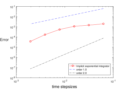
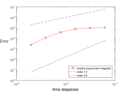
Figure 1: Strong convergence rates of the temporal discretization given by the implicit exponential Euler scheme (IEE) (left: $d=1$, right: $d=2$).

We now fix $N=100$ for $d=1$ and $N=30$ for $d=2$ and investigate the strong convergence rates in time by using the stepsizes $\tau=2^{-j},j=4,5,\ldots,9$. The reference solution is computed numerically by using the proposed time integrator with the reference stepsize $\tau=2^{-10}$. In the loglog plots from Figure 1, one can observe that the approximation errors of the implicit exponential Euler scheme decrease with order $1$. This is consistent with our theoretical findings.

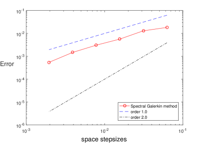
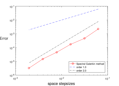
Figure 2: Strong convergence rates of the spatial discretization given by the spectral Galerkin method (left: $L^{2}(\Omega;\mathbb{H}^{1})$ error, right: $L^{2}(\Omega;\mathbb{H})$ error).

To visually illustrate the error in space for $d=1$, we compute a reference solution by using the proposed numerical scheme with $\tau=2^{-5}$ and $N=2^{10}$. The resulting errors of six different mesh parameters $N=2^{i},i=4,5,\ldots,9$ are plotted in Figure 2 on a log–log scale. One can observe that the expected convergence rates agree with those indicated in Theorem 3.2 and Theorem 3.4.

References

- [1] R. A. Adams. Sobolev Spaces, Pure and Applied Mathematics, Volume 65, Elsevier, Amsterdam, 1975.
- [2] R. Anton, D. Cohen, S. Larsson and X. Wang. Full discretisation of semi-linear stochastic wave equations driven by multiplicative noise. SIAM J. Numer. Anal., 54(2):1093–1119, 2016.
- [3] V. Barbu, G. Da Prato. The stochastic nonlinear damped wave equation. Appl. Math. Optim., 46(2-3):125–141, 2002.
- [4] V. Barbu, G. Da Prato and L. Tubaro. Stochastic wave equations with dissipative damping. Stochastic Process. Appl., 117(8):1001–1013, 2007.
- [5] S. Becker, B. Gess, A. Jentzen and P. E. Kloeden. Strong convergence rates for explicit space-time discrete numerical approximations of stochastic Allen–Cahn equations. Stoch. Partial Differ. Equ. Anal. Comput., 11(1):211–268, 2023.
- [6] D. Blomker and A. Jentzen. Galerkin approximations for the stochastic Burgers equation. SIAM J. Numer. Anal., 51(1):694–715, 2013.
- [7] C.-E. Bréhier, J. Cui and J. Hong. Strong convergence rates of semi-discrete splitting approximations for stochastic Allen–Cahn equation. IMA J. Numer. Anal., 39(4):2096–2134, 2019.
- [8] C.-E. Bréhier, M. Hairer and A. M. Stuart. Weak error estimates for trajectories of SPDEs under spectral Galerkin discretization. J. Comput. Math., 36(2):159–182, 2018.
- [9] E. M. Cabaña. On barrier problems for the vibrating string. Probab. Theory Related Fields, 22:13–24, 1972.
- [10] M. Cai, S. Gan and X. Wang. Weak convergence rates for an explicit full-discretization of stochastic Allen–Cahn equation with additive noise. J. Sci. Comput., 86:34, 2021.
- [11] S. Campbell and G. J. Lord. Adaptive time-stepping for stochastic partial differential equations with non-Lipschitz drift. arXiv preprint arXiv:1812.09036, 2018.
- [12] Y. Cao and L. Yin. Spectral Galerkin method for stochastic wave equations driven by space-time white noise. Commun. Pure Appl. Anal., 6(3):607–617, 2007.
- [13] P.-L. Chow. Asymptotics of solutions to semilinear stochastic wave equations. Ann. Appl. Probab., 16(2):757–789, 2006.
- [14] D. Cohen and A. Lang. Numerical approximation and simulation of the stochastic wave equation on the sphere. Calcolo, 59:32, 2022.
- [15] D. Cohen, S. Larsson and M. Sigg. A trigonometric method for the linear stochastic wave equation. SIAM J. Numer. Anal., 51(1):204–222, 2013.
- [16] D. Cohen and L. Quer-Sardanyons. A fully discrete approximation of the one-dimensional stochastic wave equation. IMA J. Numer. Anal., 36(1):400–420, 2016.
- [17] J. Cui and J. Hong. Strong and weak convergence rates of finite element method for stochastic partial differential equation with non-globally Lipschitz coefficients. SIAM J. Numer. Anal., 57(4):1815–1841, 2019.
- [18] J. Cui, J. Hong, L. Ji and L. Sun. Energy-preserving exponential integrable numerical method for stochastic cubic wave equation with additive noise. arXiv preprint arXiv:1909.00575, 2019.
- [19] J. Cui, J. Hong and L. Sun. Semi-implicit energy-preserving numerical schemes for stochastic wave equation via SAV approach. arXiv preprint arXiv:2208.13394, 2022.
- [20] R. C. Dalang, D. Khoshnevisan, C. Mueller, D. Nualart and Y. Xiao. A Minicourse on Stochastic Partial Differential Equations. Volume 152. Lecture Notes in Math. 1962, Springer-Verlag, Berlin, 2009.
- [21] G. Da Prato and J. Zabczyk. Stochastic Equations in Infinite Dimensions. Volume 152. Cambridge university press, 2014.
- [22] X. Feng, Y. Li and Y. Zhang. Finite element methods for the stochastic Allen–Cahn equation with gradient-type multiplicative noise. SIAM J. Numer. Anal., 55(1):194–216, 2017.
- [23] H. Gao, F. Liang, and B. Guo. Stochastic wave equations with nonlinear damping and source terms. Infin. Dimens. Anal. Quantum Probab. Relat. Top., 16(2):1350013-1–1350013-29, 2013.
- [24] I. Gyöngy, S. Sabanis and D. Šiška. Convergence of tamed Euler schemes for a class of stochastic evolution equations. Stoch. Partial Differ. Equ. Anal. Comput., 4(2):225–245, 2016.
- [25] J. U. Kim. On the stochastic wave equation with nonlinear damping. Appl. Math. Optim., 58(1):29–67, 2008.
- [26] K. Klioba and M. Veraar. Pathwise uniform convergence of time discretisation schemes for SPDEs. arXiv preprint arXiv:2303.00411, 2023.
- [27] M. Kovács, A. Lang and A. Petersson. Weak convergence of fully discrete finite element approximations of semilinear hyperbolic SPDE with additive noise. ESAIM Math. Model. Numer. Anal., 54(6):2199–2227, 2020.
- [28] M. Kovács, S. Larsson and F. Lindgren. Weak convergence of finite element approximations of linear stochastic evolution equations with additive noise II. Fully discrete schemes. BIT, 53(2):497–525, 2013.
- [29] M. Kovács, S. Larsson and F. Lindgren. On the backward Euler approximation of the stochastic Allen–Cahn equation. J. Appl. Probab., 52(2):323–338, 2015.
- [30] M. Kovács, S. Larsson and F. Saedpanah. Finite element approximation of the linear stochastic wave equation with additive noise. SIAM J. Numer. Anal., 48(2):408–427, 2010.
- [31] R. Kruse. Strong and Weak Approximation of Semilinear Stochastic Evolution Equations. Springer, 2014.
- [32] Z. Lei, C.-E. Bréhier and S. Gan. Numerical approximation of the invariant distribution for a class of stochastic damped wave equations. arXiv preprint arXiv:2306.13998, 2023.
- [33] Y. Li, S. Wu and Y. Xing. Finite element approximations of a class of nonlinear stochastic wave equations with multiplicative noise. J. Sci. Comput., 91:53, 2022.
- [34] Z. Liu and Z. Qiao. Strong approximation of monotone stochastic partial differential equations driven by multiplicative noise. Stoch. Partial Differ. Equ. Anal. Comput., 9(3):559–602, 2021.
- [35] G. J. Lord, C. E. Powell and T. Shardlow. An Introduction to Computational Stochastic PDEs. Number 50. Cambridge University Press, 2014.
- [36] R. Qi and X. Wang. An accelerated exponential time integrator for semi-linear stochastic strongly damped wave equation with additive noise. J. Math. Anal. Appl., 447(2):988–1008, 2017.
- [37] R. Qi and X. Wang. Error estimates of finite element method for semi-linear stochastic strongly damped wave equation. IMA J. Numer. Anal., 39(3):1594–1626, 2019.
- [38] R. Qi. and X. Wang. Optimal error estimates of Galerkin finite element methods for stochastic Allen–Cahn equation with additive noise. J. Sci. Comput., 80(2):1171–1194, 2019.
- [39] L. Quer-Sardanyons and M. Sanz-Solé. Space semi-discretisations for a stochastic wave equation. Potential Anal., 24(4):303–332, 2006.
- [40] H. Schurz. Analysis and discretization of semi-linear stochastic wave equations with cubic nonlinearity and additive space-time noise. Discrete Contin. Dyn. Syst. Ser. S, 1(2):353–363, 2008.
- [41] A. Stuart and A. Humphries. Dynamical Systems and Numerical Analysis. Cambridge University Press, Cambridge, 1996.
- [42] V. Thomée. Galerkin Finite Element Methods for Parabolic Problems. Springer, Berlin, 2006.
- [43] J. B. Walsh. On numerical solutions of the stochastic wave equation. Illinois J. Math., 50(1-4):991–1018, 2006.
- [44] X. Wang. An exponential integrator scheme for time discretization of nonlinear stochastic wave equation. J. Sci. Comput., 64(1):234–263, 2015.
- [45] X. Wang. An efficient explicit full-discrete scheme for strong approximation of stochastic Allen–Cahn equation. Stochastic Process. Appl., 130(10):6271–6299, 2020.
- [46] X. Wang, S. Gan and J. Tang. Higher order strong approximations of semilinear stochastic wave equation with additive space-time white noise. SIAM J. Sci. Comput., 36(6):A2611–A2632, 2014.
- [47] X. Wang, J. Wu and B. Dong. Mean-square convergence rates of stochastic theta methods for SDEs under a coupled monotonicity condition. BIT, 60(3):759–790, 2020.