Emergent non-Markovianity and dynamical quantification of the quantum switch

Abstract

We investigate the dynamical aspects of the quantum switch and find a particular form of quantum memory emerging out of the switch action. We first analyse the loss of information in a general quantum evolution subjected to a quantum switch and propose a measure to quantify the switch-induced memory. We then derive an uncertainty relation between information loss and switch-induced memory. We explicitly consider the example of depolarising dynamics and show how it is affected by the action of a quantum switch. For a more detailed analysis, we consider both the control qubit and the final measurement on the control qubit as noisy and investigate the said uncertainty relation. Further, while deriving the Lindblad-type dynamics for the reduced operation of the switch action, we identify that the switch-induced memory actually leads to the emergence of non-Markovianity. Interestingly, we demonstrate that the emergent non-Markovianity can be explicitly attributed to the switch operation by comparing it with other standard measures of non-Markovianity. Our investigation thus paves the way forward to understanding the quantum switch as an emerging non-Markovian quantum memory.

I Introduction

The superposition principle allows for multiple simultaneous evolutions, creating potential advantages in several quantum communication and quantum key distribution protocols by refining the effect of noise Gisin et al. (2005). Usually, even in quantum scenarios, the information carriers or channels are arranged in well-defined classical configurations. However, with an external control system called the quantum switch (QS) Chiribella et al. (2013), the causal order of multiple quantum evolutions or quantum channels can be put in superposition to create an indefinite causal order. For an illustration, let us consider two quantum channels, $\mathcal{N}_{1}$ and $\mathcal{N}_{2}$, and a quantum state $\rho$. A control qubit determines the order of action of the two channels on $\rho$. When the control qubit is in the state $\ket{0}$, first $\mathcal{N}_{1}$ acts on $\rho$ followed by $\mathcal{N}_{2}$: $\left(\mathcal{N}_{2}\circ\mathcal{N}_{1}\right)(\rho)$. The order is reversed when the control qubit is in the state $\ket{1}$, i.e., $\left(\mathcal{N}_{1}\circ\mathcal{N}_{2}\right)(\rho)$. Hence, if the control qubit is prepared in the superposition state, $\ket{+}$ or $\ket{-}$ (where $\ket{\pm}\equiv(\ket{0}\pm\ket{1})/\sqrt{2}$), we get a superposition of the causal orders of the actions of the two channels.

Indefiniteness in the order of quantum operations is beneficial over the standard quantum Shannon theory in several aspects. For example, it is better in testing the properties of quantum channel Chiribella (2012), winning non-local games Oreshkov et al. (2012), achieving quantum computational advantages Araújo et al. (2014), minimising quantum communication complexity Guérin et al. (2016), improving quantum communication Ebler et al. (2018); Chiribella et al. (2021); Bhattacharya et al. (2021), enhancing the precision of quantum metrology Zhao et al. (2020), or providing thermodynamic advantages Guha et al. (2020); Felce and Vedral (2020); Maity and Bhattacharya (2022), etc. (also see Mukhopadhyay and Pati (2020); Ghosal et al. (2023)). Recently, a second quantised Shannon theory has also been proposed Kristjánsson et al. (2020). Several of these advantages have already been ascertained in experiments et al. (2015); al (2017); Goswami et al. (2018). Because of the enormous application potential, in the literature, more attention has been paid to the applicability of the QS in quantum information-theoretic and communication protocols and its advantages than its dynamical aspects. Here, however, we mainly focus on the dynamical aspects of the QS and find a form of quantum memory that emerges from the QS dynamics. This is important since quantum memory is crucial for future developments of quantum technologies in long-distance quantum communications Chang et al. (2019); Duan et al. (2001), enhancing the capacity of long quantum channels Kretschmann and Werner (2005); D'Arrigo et al. (2007); Datta and Dorlas (2009); Bylicka et al. (2014), or improving the efficiency of thermodynamic machines Bylicka et al. (2016); Taranto et al. (2020, 2023), etc. We also establish that the QS-induced memory (QSM) is equivalent to the non-Markovianity emerging from the resultant dynamics.

Since the past decade, quantum Non-Markovian processes are interpreted as a form of quantum memory in dynamical processes Breuer et al. (2004); Laine et al. (2010); Rivas et al. (2010, 2014); Vasile et al. (2011); Lu et al. (2010); Luo et al. (2012); Fanchini (2014); Chanda and Bhattacharya (2016); Haseli (2014); Mukhopadhyay et al. (2017); Bhattacharya et al. (2020a, b); Maity et al. (2020); Bhattacharya and Bhattacharya (2021); Bhattacharya et al. (2018); Das et al. (2021); Giarmatzi and Costa (2021); Mallick et al. (2023). In the theory of open quantum systems Alicki and Lendi (2007), the system is generally assumed to couple weakly to a static environment without any memory of the past, leading to memoryless Markovian processes. This gives rise to a one-way information flow from the system to the environment. However, in realistic scenarios, such an ideal assumption does not hold, and, almost always, there is some non-Markovian backflow of information from the environment to the system. The backflow behaves like a memory providing advantages in information processing, communication and computational tasks over the memoryless or Markovian operations Laine et al. (2014); Bylicka et al. (2014); Xiang et al. (2014); Thomas et al. (2018); Reich et al. (2015). There could be multiple reasons behind the occurrence of non-Markovianity, e.g., the strength of the system-environment interaction, the nature of the bath state, etc. Therefore, the system-environment interaction is one of the key resources for triggering such non-Markovian dynamics Breuer and Petruccione (2002); Rivas et al. (2014); de Vega and Alonso (2017); Breuer et al. (2016). Naturally, the QS also allows us to create and regulate the effect of non-Markovianity by manipulating the interaction between the environment and the system degrees of freedom via the control qubit. Hence, considering the control qubit to be a part of the environment, we can interpret that the emergent memory is stemming from a carefully controlled system-environment coupling. The ability to control memory effects by manipulating the system-environment interaction is beneficial in several information-processing tasks. For example, it creates potential advantages over classical technology Chiribella et al. (2008, 2009); White et al. (2020), enhances the efficiencies of thermodynamic machines Bylicka et al. (2016); Taranto et al. (2020, 2023), preserves coherence and quantum correlation Barreiro et al. (2010), allows the implementation of randomised benchmarking and error correction Ball et al. (2016); Figueroa-Romero et al. (2021, 2022) or performing optimal dynamical decoupling Addis et al. (2015); Biercuk et al. (2009), etc.

In this paper, we investigate the dynamics of QS and characterise the non-Markovian memory emerging from it. We look at the information loss Awasthi et al. (2018) in an ergodic Markovian-quantum evolution under the QS. The notion of ergodic quantum operations stems from the well-known ergodic hypothesis, according to which a system evolving under the influence of a static environment over a sufficiently long time will always evolve to a steady state, whose properties depend on the environment and the nature of the interaction. For example, in the case of thermal environments, the system will deterministically evolve to a thermal state with the same temperature as the environment. In quantum scenarios, it implies that ergodic quantum operations have a singular fixed point or, in other words, a particular steady state. For our purpose, we choose a generic Markovian operation satisfying the ergodicity property for the evolution operation on which a QS is applied.

The information loss at a time $t$ can be measured by the difference of the geometric distances between two states at $t$ and initially. Even though the difference never decreases with time for memoryless dynamics Awasthi et al. (2018), it does so under a QS. This indicates a non-trivial relation between the information loss for a given dynamics under a QS and the QSM. We show that the sum of the information loss and the QSM is actually lower-bounded by the distance between the initial states. We consider a special case of the generalised Pauli channel (depolarising channel) and investigate the dynamical evolution. We find that under the action of QS, it allows reverse information transmission from the environment to the system. We prove that the information-carrying capability of the completely depolarising channel under QS is due to the induced non-Markovianity from the switch operation alone, and not due to the convex combination of two separate evolutions. For completeness, we also quantify the amount of noise a QS can tolerate. We introduce noise at both the control qubit and the final measurement on the control bit and investigate how the system evolutions get affected by the noises.

Further, we analyse non-Markovian quantum operations from their divisibility perspective Rivas et al. (2010). Divisible quantum operations are those which can be perceived as a sequence of an arbitrary number of completely positive trace-preserving (CPTP) dynamical maps acting on a quantum system. Whereas, non-divisible operations elucidate the information backflow Laine et al. (2010); Breuer et al. (2009), which can be perceived as a sufficient benchmark of the presence of non-Markovian memory in the concerning quantum operation.

The paper is organised as follows. In the next section, we briefly introduce the QS. In Section III, we evaluate the information loss of general quantum evolution with or without the QS, define the QSM measures and derive their relation. Further, we define the ergodic quantum channel formally and prove some relevant statements as a consolidated backdrop for our investigation. In section IV, we investigate the dynamical evolution under QS. We then explore how the QS behaves in the presence of various possible noises and investigate its tolerance against them. In section V, we derive a Lindbald-type master equation for qubit depolarizing dynamics subjected to QS and investigate how non-Markovianity emerges out of QS dynamics from the perspective of a qubit evolution. We then find interesting connections between the QS with some well-known measures of non-Markovianity. Finally, in Section VI, we conclude and remark about possible future directions.

II Quantum SWITCH

A quantum channel $\mathcal{N}$ between systems $A$ and $B$ is a completely positive trace-preserving map from $L(\mathcal{H}_{A})$ to $L(\mathcal{H}_{B})$, where $\mathcal{H}_{A}$ and $\mathcal{H}_{B}$ are the Hilbert spaces corresponding to the input system $A$ and the output system $B$, respectively, and $L(\mathcal{H}_{i})$ are the set of bounded linear operators on $\mathcal{H}_{i}$. The action of $\mathcal{N}$ on an input state $\rho\in L(\mathcal{H}_{A})$ can be expressed in the Kraus representation (operator-sum representation) form as $\mathcal{N}(\rho)=\sum_{i}K_{i}\rho K_{i}^{\dagger}$, where $\{K_{i}\}$ are the Kraus operators for $\mathcal{N}$. If there are two channels, $\mathcal{N}_{1}$ and $\mathcal{N}_{2}$, they can act either in parallel or in series. The parallel action of the channels can be realised as $\mathcal{N}_{1}\otimes\mathcal{N}_{2}$. The series actions can be realised in more than one way: $\mathcal{N}_{1}$ followed by $\mathcal{N}_{2}$ (denoted by $\mathcal{N}_{2}\circ\mathcal{N}_{1}$) or $\mathcal{N}_{2}$ followed by $\mathcal{N}_{1}$ (denoted by $\mathcal{N}_{1}\circ\mathcal{N}_{2}$). If the causal order is definite, then among these two possibilities, any one of either $\mathcal{N}_{2}\circ\mathcal{N}_{1}$ or $\mathcal{N}_{1}\circ\mathcal{N}_{2}$ is allowed. However, as mentioned in the Introduction, the order of the action of two channels can be made indefinite with an additional ancillary system called the control qubit ($\omega_{c}$) Ebler et al. (2018); Chiribella et al. (2021); Bhattacharya et al. (2021). When $\omega_{c}$ is initialised in the $\ket{0}\bra{0}$ state, the $\mathcal{N}_{2}\circ\mathcal{N}_{1}$ configuration acts on the state $\rho$, whereas the $\mathcal{N}_{1}\circ\mathcal{N}_{2}$ configuration acts when $\omega_{c}$ is initialised in the $\ket{1}\bra{1}$ state. If ${K^{(1)}_{i}}$ represents the Kraus operator for $\mathcal{N}_{1}$ and ${K^{(2)}_{j}}$ for $\mathcal{N}_{2}$, the general Kraus operator can be represented as

$$S_{ij}=K_{j}^{(2)}\circ K_{i}^{(1)}\otimes|0\rangle_{c}\left\langle{}_{{c\hskip 2.00749pt}}0\right|+K_{i}^{(1)}\circ K_{j}^{(2)}\otimes|1\rangle_{c}\left\langle{}_{{c\hskip 2.00749pt}}1\right|.$$ (1)

The overall evolution of the combined system can be written as

$$S\left(\mathcal{N}_{1},\mathcal{N}_{2}\right)\left(\rho\otimes\omega_{c}\right)=\sum_{i,j}S_{ij}\left(\rho\otimes\omega_{c}\right)S_{ij}^{\dagger}.$$ (2)

In the end, the control qubit is measured on the coherent basis $\{\ket{+}\bra{+},\ket{-}\bra{-}\}$. Then, for each outcome, the reduced state corresponding to the target qubit becomes,

$${}_{c}\bra{\pm}S(\mathcal{N}_{1},\mathcal{N}_{2})(\rho\otimes\omega_{c})\ket{\pm}_{c}.$$ (3)

This is essentially how the QS works, as we show schematically in Fig. 1.

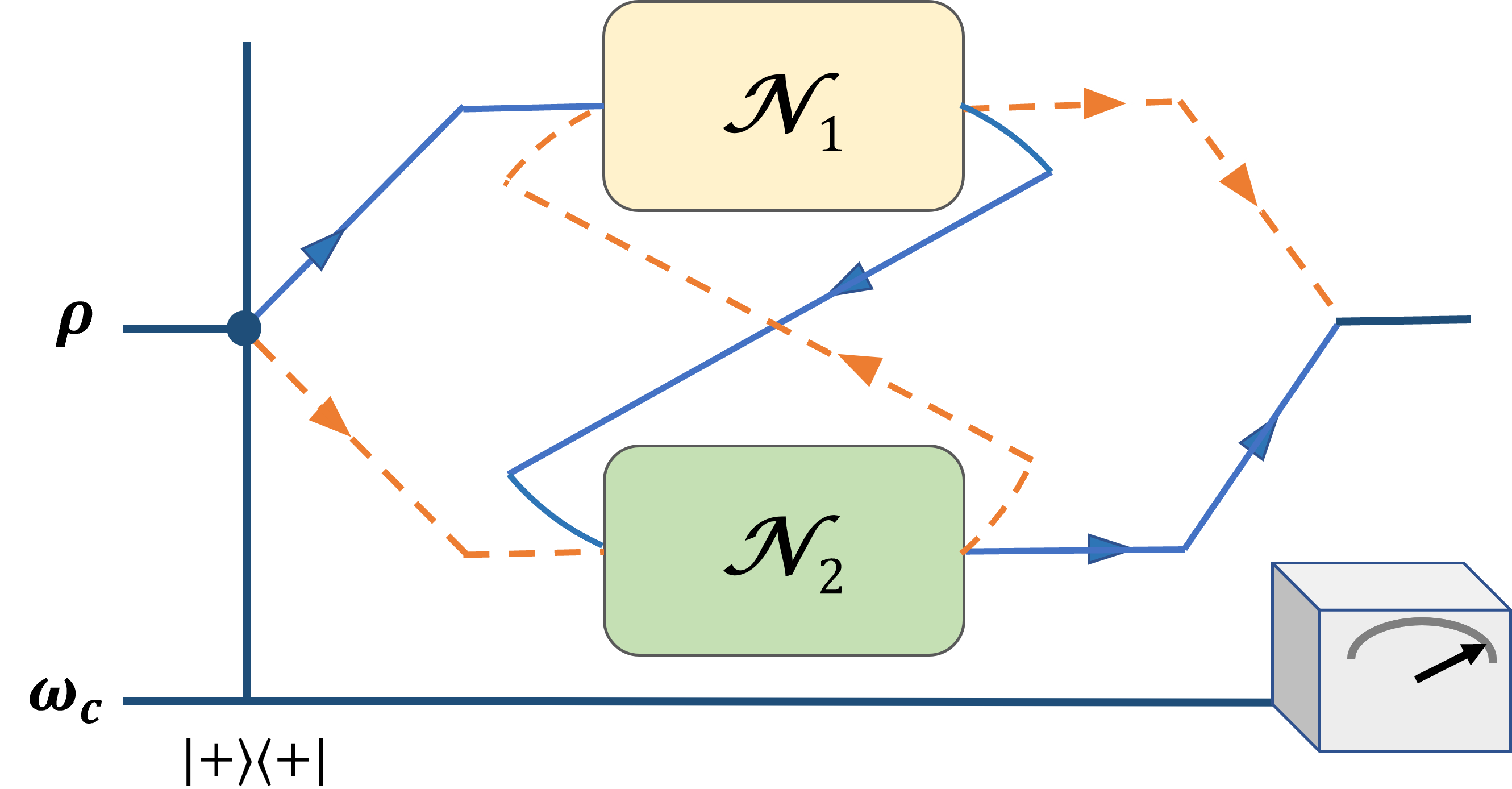
Figure 1: The quantum switch. When the control qubit $\omega_{c}$ is prepared in $\ket{0}\bra{0}$ state, the state $\rho$ can evolve first through channel $\mathcal{N}_{1}$ and then through $\mathcal{N}_{2}$ (the blue solid line) and when the control qubit is prepared in $\ket{1}\bra{1}$ state, the state $\rho$ can evolve first through channel $\mathcal{N}_{2}$ and then through $\mathcal{N}_{1}$ (the orange dotted line). However, when the control qubit is prepared in $\ket{+}\bra{+}$ state, the order of the action of two channels is in superposition. Finally, the control qubit is measured in $\{\ket{\pm}\bra{\pm}\}$ basis.

III Information Loss and the Measure of quantum SWITCH

Before proceeding further, we need to introduce some basic concepts, like the notion of time-averaged quantum states and ergodic evolution, to understand the relationship between information loss and the QSM. The ergodic hypothesis of statistical mechanics states that if a physical system (be it classical or quantum) evolves over a long period, the time-averaged state of the system will be equal to its thermal state with a temperature equal to that of the bath, with which the system was interacting. In other words, for an observable $f$, if the (long-)time average $\langle f\rangle_{t}$ is equal to the ensemble average $\langle f\rangle_{\text{ens}}$ over the equilibrium state, the system is ergodic. If a quantum operation $\Phi_{t}(\cdot)$ acts on a state $\rho$ from $t=0$ to $t=T$, we can express the long-time-averaged state as

$$\overline{\Phi_{t}(\rho)}=\lim_{T\to\infty}\frac{1}{T}\int_{0}^{T}\Phi_{t}(\rho)\;dt.$$ (4)

Long-time averaging of any observable can thus be defined in the Schrödinger picture as

$$\langle f\rangle_{\infty} =\lim_{T\to\infty}\frac{1}{T}\int_{0}^{T}\text{Tr}\left[f\Phi_{t}(\rho)\right]dt$$

$$=\text{Tr}\left[f\left(\lim_{T\to\infty}\frac{\int_{0}^{T}\Phi_{t}(\rho)dt}{T}\right)\right]$$

$$=\text{Tr}[f\;\overline{\Phi_{t}(\rho)}].$$ (5)

We now define the ergodic evolution as follows (Burgarth et al., 2013; Awasthi et al., 2018).

$\blacksquare$ Definition 1: A quantum evolution is ergodic if it has a singular fixed point and the time-averaged state equals that fixed point.

A dynamics or quantum evolution is said to possess a singular fixed point if there exists exactly one state that remains unaffected by the quantum evolution—for example, a depolarising channel with the maximally mixed state, a thermal channel with the thermal state, an amplitude damping channel with the ground state, etc. Thus, if $\tau$ is the singular fixed point of a given quantum channel $\Phi_{t}(\cdot)$, i.e., if $\Phi_{t}(\tau)=\tau$, the channel is called ergodic if $\overline{\Phi_{t}(\rho)}=\tau$ for an arbitrary initial state $\rho$. We denote such channels as $\Phi^{\epsilon}_{t}(\cdot)$. In Appendix A, we present an example of a qubit ergodic Pauli channel, which is relevant to our study. Note that, by definition, ergodic quantum channels are the true memoryless channels since the time-averaged states do not depend on the initial state at all.

For some channels, the singular fixed point $\tau$ remains unaltered even under the action of a QS. If we denote the action of such channels as $\Phi^{S}_{t}(.)$, then $\Phi^{S}_{t}(\tau)=\tau$. Below, we prove that such a condition is true even for generalised Pauli channels in arbitrary dimensions.

$\blacksquare$ Statement 1: For generalized Pauli channels in arbitrary dimensions, their singular fixed point (maximally mixed state) remains unchanged under the action of the quantum switch.

Proof.

The generalized Pauli channel for a $d$-dimensional quantum system can be represented by the following map (Chruściński and Siudzińska, 2016),

$$\Lambda_{W}(\rho)=\sum_{k,l=0}^{d-1}p_{kl}W_{kl}\rho W_{kl}^{\dagger}$$ (6)

where $W_{kl}=\sum_{m=0}^{d-1}\omega^{mk}\ket{m}\bra{m+l}$ with $\omega=e^{2\pi i/d}$ are the unitary Weyl operators. The Weyl operators satisfy the following well-known properties:

$$W_{kl}W_{rs}=\omega^{ks}W_{k+r,l+s}~{}~{}\text{and}~{}~{}W_{kl}^{\dagger}=\omega^{kl}W_{-k,-l}$$ (7)

where the indices are modulo-$d$ integers. For such channels, the maximally mixed state $\frac{\mathbb{I}}{d}$ is the fixed point. We show that the maximally mixed state remains the fixed point after the action of the QS. The reduced representation of the action of the QS over a generalised Pauli channel can be written as

$$\Lambda_{W}^{S}(\rho)= \frac{\sum_{k,l,r,s}\widetilde{W}_{klrs}\rho\widetilde{W}_{klrs}^{\dagger}}{\text{Tr}\left[\rho\sum_{k,l,r,s}\widetilde{W}_{klrs}^{\dagger}\widetilde{W}_{klrs}\right]},$$ (8)

$${\text{ with}}\ \ \ \ \ \widetilde{W}_{klrs}= \frac{\sqrt{p_{kl}p_{rs}}}{2}(W_{kl}W_{rs}+W_{rs}W_{kl})~{}\mbox{(see Appendix~{}\ref{sec:appkraus})}.$$

Using these relations and the properties of dummy indices $k,l,r,s$, we get

$$\sum_{k,l,r,s}\widetilde{W}_{klrs}\frac{\mathbb{I}}{d}\widetilde{W}_{klrs}^{\dagger} =\frac{1}{d}\sum_{k,l,r,s}\widetilde{W}_{klrs}\widetilde{W}_{klrs}^{\dagger}$$

$$=\frac{1}{2d}\sum_{k,l,r,s}p_{kl}p_{rs}(1+\omega^{ks-rl})\mathbb{I}.$$ (9)

Therefore,

$$\Lambda_{W}^{S}\left(\frac{\mathbb{I}}{d}\right)=\frac{\frac{1}{d}\sum_{k,l,r,s}p_{kl}p_{rs}(1+\omega^{ks-rl})\mathbb{I}}{\sum_{k,l,r,s}p_{kl}p_{rs}(1+\omega^{ks-rl})}=\frac{\mathbb{I}}{d},$$ (10)

which proves the statement. ∎

We use the ergodic generalised Pauli channel in our further analysis.

III.1 Uncertainty relation between QS-induced memory and information loss

Let $D(\rho_{1},\rho_{2})$ be the geometric distance between two states $\rho_{1}$ and $\rho_{2}$ satisfying the necessary properties of a distance measure, i.e., it is symmetric, non-negative and obeys the triangular inequality. In particular, if $D(\rho_{1},\rho_{2})$ is the trace distance measure then $D(\rho_{1},\rho_{2})\equiv\frac{1}{2}||\rho_{1}-\rho_{2}||_{1}$, where $||A||_{1}=\text{Tr}[\sqrt{A^{\dagger}A}]$. Now, under any noisy evolution $\Phi_{t}$, the distance between two states can never increase where the final distance depends on the nature of the evolution. With this in mind, we define the following quantity.

$\blacksquare$ Definition 2: If $\rho_{1}(0)$ and $\rho_{2}(0)$ are two initial states evolving under $\Phi_{t}(\cdot)$, the quantity $\Delta\mathcal{I}(\rho_{1}(t),\rho_{2}(t))$, defined as

$$\Delta\mathcal{I}(\rho_{1}(t),\rho_{2}(t))\equiv \ D(\rho_{1}(0),\rho_{2}(0))$$

$$\ -D(\Phi_{t}(\rho_{1}(0)),\Phi_{t}(\rho_{2}(0))),$$ (11)

is a measure of the information loss across the channel.

The quantity $\Delta\mathcal{I}(\rho_{1}(t),\rho_{2}(t))$ quantifies the difference between the initial distinguishability of the two states and their distinguishability after the action of the noisy evolution $\Phi_{t}$. If we consider an ergodic operation $\Phi_{t}^{\epsilon}(\cdot)$ with a singular fixed point $\tau$ and take $\rho_{1}(0)=\rho$ and $\rho_{2}(0)=\tau$ then the information loss becomes

$$\Delta\mathcal{I}_{\epsilon}(\rho(t))=D(\rho,\tau)-D(\Phi_{t}^{\epsilon}(\rho),\tau),$$ (12)

since $\tau$ remains unaffected by the evolution. Now, if $\tau$ is also a fixed point under QS, then the information loss under the QS dynamics will be

$$\Delta\mathcal{I}_{S}(\rho(t))=D(\rho,\tau)-D(\Phi_{t}^{S}(\rho),\tau).$$ (13)

We can now define the QS-induced memory as follows.

$\blacksquare$ Definition 3: The QS-induced memory (QSM), $\mathcal{Q}_{s}$, can be defined as

$$\mathcal{Q}_{S}(t)\equiv D(\Phi^{S}_{t}(\rho),\Phi_{t}^{\epsilon}(\rho)).\\$$ (14)

Clearly, when the evolution $\Phi(\cdot)$ is unaffected by the switch, $\Phi^{S}_{t}=\Phi_{t}^{\epsilon}$ and hence $\mathcal{Q}_{S}$ will be zero.

We can relate $\Delta\mathcal{I}_{S}(\rho(t))$ with $\Delta\mathcal{I}_{\epsilon}(\rho(t))$ as

$$\Delta\mathcal{I}_{S}(\rho(t))= \ D(\rho,\tau)-D(\Phi^{S}_{t}(\rho),\tau)$$

$$= \ D(\rho,\tau)-D(\Phi^{S}_{t}(\rho)-\Phi_{t}^{\epsilon}(\rho),\tau-\Phi_{t}^{\epsilon}(\rho))$$

$$\geq \ D(\rho,\tau)-D(\Phi^{S}_{t}(\rho),\Phi_{t}^{\epsilon}(\rho))-D(\Phi_{t}^{\epsilon}(\rho),\tau)$$

$$\geq \ D(\rho,\tau)-\mathcal{Q}_{S}(t)-D(\Phi_{t}^{\epsilon}(\rho),\tau),$$

which implies,

$$\Delta\mathcal{I}_{S}(\rho(t))+\mathcal{Q}_{S}(t)\geq\Delta\mathcal{I}_{\epsilon}(\rho(t)).$$ (15)

Here, we have used the triangle inequality: $D(A,B)+D(B,C)\geq D(C,A)$ and the symmetric property of the distance measure: $D(A,B)=D(B,A)$. The uncertainty relation between the information loss and the QSM in Eq. (15) is one of the main results of this paper. We will refer to it as the quantum switch-induced information inequality (QSI) later.

If we evaluate these measures for the time-averaged states under the QS, the information loss and the QSM measure reduce to

$$\Delta\overline{\mathcal{I}}_{S}=D(\rho,\tau)-D(\overline{\Phi^{S}_{t}(\rho)},\tau)$$ (16)

and

$$\overline{\mathcal{Q}}_{S}=D(\overline{\Phi^{S}_{t}(\rho)},\overline{\Phi_{t}^{\epsilon}(\rho)})=D(\overline{\Phi^{S}_{t}(\rho)},\tau),$$ (17)

respectively, and the QSI in Eq. (15) reduces to an equality:

$$\Delta\overline{\mathcal{I}}_{S}+\overline{\mathcal{Q}}_{S}=D(\rho,\tau)=\Delta\overline{\mathcal{I}}_{\epsilon}.$$ (18)

The above equation indicates that as the QSM increases, the information loss decreases and hence, the QS is a resource for information storage undergoing noisy quantum operations.

IV Dynamical evolution under the action of quantum SWITCH and emergence of non-Markovianity

In this section, we study an explicit example of dynamical evolution and investigate how the evolution changes under the action of the QS. We analyse the QSM (1) from the perspective of non-Markovianity by deriving the Lindblad-type generator for the switch operation and (2) from the point of view of non-ergodicity as proposed in the previous section. For this purpose, we consider qubit depolarising operation as described below.

IV.1 Evolution under completely depolarizing dynamics in a definite causal structure

We choose the Markovian qubit-depolarising channel for the case study. We call a channel Markovian if it is completely positive (CP) divisible. A dynamical map $\Phi_{(t,t_{0})}$ is said to be CP divisible if it can be represented as $\Phi_{(t,t_{0})}=\Phi_{(t,t_{s})}\circ\Phi_{(t_{s},t_{0})}$, $\forall t_{s}$ with $t_{0}\leq t_{s}\leq t$ and $\Phi_{(t,t_{s})}$ is completely positive. The notation $\Phi_{(t,t_{s})}$ means the quantum channel $\Phi(\cdot)$ acts for the time period $t_{s}$ to $t$. When $t_{0}=0$, we abbreviate the notation as $\Phi_{t}$, as in the previous section. Note that there are various other criteria for identifying quantum non-Markovianity in the literature, of which information backflow Laine et al. (2010); Breuer et al. (2009) is relevant for our discussion. Information backflow is the reverse information flow from the environment to the system, mathematically quantified by the anomalous non-monotonic behaviours of known monotones (like the trace distance between two states) under dynamical evolution Laine et al. (2010). It is well-known that breaking CP-divisibility is a necessary condition for information backflow, but not vice versa.

We consider a CP-divisible map $\Phi_{t}$ possessing a Lindblad-type generator $\mathcal{L}_{t}$, i.e., $\Phi_{t}\equiv\exp{\left(\int_{0}^{t}\mathcal{L}_{s}ds\right)}$. The generator of the dynamics can be expressed as,

$$\frac{d}{dt}\rho(t)=\mathcal{L}_{t}(\rho(t)),$$ (19)

where

$$\mathcal{L}_{t}(X)=\sum_{i}\Gamma_{i}(t)\left(A_{i}XA_{i}^{\dagger}-\frac{1}{2}\left\{A_{i}^{\dagger}A_{i},X\right\}\right)$$

with $\Gamma_{i}(t)$ being the Lindblad coefficients and $A_{i}$, the Lindblad operators. The necessary and sufficient condition for an operation being CP divisible is that all the Lindblad coefficients $\Gamma_{i}(t)$ are positive $\forall(i,t)$ Lindblad (1976); Gorini et al. (1976). For our purpose, the evolution of a system under definite causal order is considered to be Markovian.

Starting with a definite causal order, we consider the following master equation,

$$\frac{d}{dt}\rho(t)=\sum_{i=1}^{3}\gamma_{i}(t)\left[\sigma_{i}\rho(t)\sigma_{i}-\rho(t)\right]$$ (20)

where $\gamma_{i}(t)$ are the Lindblad coefficients and $\sigma_{i}$ are the Pauli matrices. The qubit is represented by

$$\Phi_{t}(\rho)\equiv\rho(t)=\left(\begin{array}[]{ll}\rho_{11}(t)&\rho_{12}(t)\\ \rho_{21}(t)&\rho_{22}(t)\end{array}\right).$$ (23)

For the completely depolarizing channel, the corresponding dynamics are represented by a CP trace-preserving dynamical map,

$$\rho_{11}(t)= \ \rho_{11}(0)\left(\frac{1+e^{-2\xi_{1}(t)}}{2}\right)+\rho_{22}(0)\left(\frac{1-e^{-2\xi_{1}(t)}}{2}\right),$$

$$\rho_{22}(t)= \ 1-\rho_{11}(t),\quad\rho_{12/21}(t)=\ \rho_{12/21}(0)e^{-2\xi_{2}(t)},$$ (24)

with

$$\xi_{1}(t)= \ \int_{0}^{t}\left[\gamma_{1}(s)+\gamma_{2}(s)\right]ds\quad\text{and}$$

$$\xi_{2}(t)= \ \int_{0}^{t}\left[\gamma_{2}(s)+\gamma_{3}(s)\right]ds.$$

The corresponding Kraus operators are given by,

$$K_{1}=\sqrt{A_{2}(t)}\left(\begin{array}[]{ll}0&1\\ 0&0\end{array}\right),\quad K_{2}=\sqrt{A_{2}(t)}\left(\begin{array}[]{ll}0&0\\ 1&0\end{array}\right),$$ (29)

$$K_{3}=\sqrt{\frac{A_{1}(t)+A_{3}(t)}{2}}\left(\begin{array}[]{cc}e^{i\theta(t)}&0\\ 0&1\end{array}\right),$$ (32)

$$K_{4}=\sqrt{\frac{A_{1}(t)-A_{3}(t)}{2}}\left(\begin{array}[]{cc}-e^{i\theta(t)}&0\\ 0&1\end{array}\right),$$ (35)

where,

$$A_{1}(t)= \ \frac{1+e^{-2\tilde{\xi}_{1}(t)}}{2},\quad A_{2}(t)=\ \frac{1-e^{-2\tilde{\xi}_{1}(t)}}{2},$$

$$A_{3}(t)= \ e^{-2\tilde{\xi}_{2}(t)},\quad\theta(t)=\ \tan^{-1}\left(\frac{\operatorname{Im}\ A_{3}(t)}{\operatorname{Re}\ A_{3}(t)}\right)=0.$$

Notice that the evolution is Markovian for the simple choice of the Lindblad coefficients, $\gamma_{1}(t)=\gamma_{2}(t)=\gamma_{3}(t)=\gamma>0$. Unless stated otherwise, we choose this set of Lindblad coefficients throughout the paper.

IV.2 Evolution under quantum switch

To see how the states evolve under the QS, we prepare two dynamical maps and put them in a superposition of causal orders with an additional control qubit, initially prepared in the $|+\rangle_{c}\left\langle{}_{{c\hskip 2.00749pt}}+\right|$ state. We consider both channels to be the same depolarising channel, i.e., $\mathcal{N}_{1}=\mathcal{N}_{2}=\mathcal{E}$. In general, the control qubit can be measured in any coherent basis but, for our purpose, we measure it in the $\left\{|\pm\rangle_{c}\left\langle{}_{{c\hskip 2.00749pt}}\pm\right|\right\}$ basis. After measuring, the state $\rho$ corresponding to the ‘$+$’ outcome can be expressed as

$$\Phi^{S}_{t}(\rho)=\frac{1}{\mathcal{A}_{1}}\left\langle{}_{{c\hskip 2.00749pt}}+\left|S\left(\rho\otimes|+\rangle_{c}\left\langle{}_{{c\hskip 2.00749pt}}+\right|\right)\right|+\right\rangle_{c}$$

$$=\ \left(\begin{array}[]{cc}A(t)\rho_{11}(0)+B(t)\rho_{22}(0)&C(t)\rho_{12}(0)\\ C(t)\rho_{21}(0)&B(t)\rho_{11}(0)+A(t)\rho_{22}(0)\end{array}\right),$$ (38)

such that $A(t)=\left(1+C(t)\right)/2$, $B(t)=\left(1-C(t)\right)/2$, and

$$C(t)= \ \frac{\mathcal{G}^{2}-2\mathcal{G}+9}{5\mathcal{G}^{2}+6\mathcal{G}-3},$$

with $\mathcal{G}=e^{4\gamma t}$. Here, $\mathcal{A}_{1}$ is the normalisation factor and the suffix ‘$c$’ represents the control qubit. In Fig. 2, we demonstrate the validity of the QSI in Eq. (15) for different values of $\gamma$. It proves the concerned QS dynamics obeys QSI perfectly. Moreover, the figure shows that initially the expression is driven away from the equality, but as time passes and the dynamics approaches the steady state, equality is reached. This, in turn, validates the equality of Eq. (18) for the long-time-averaged states. Below, we investigate the validity of this QSI for a more general situation of QS with arbitrary qubit control and measurement.

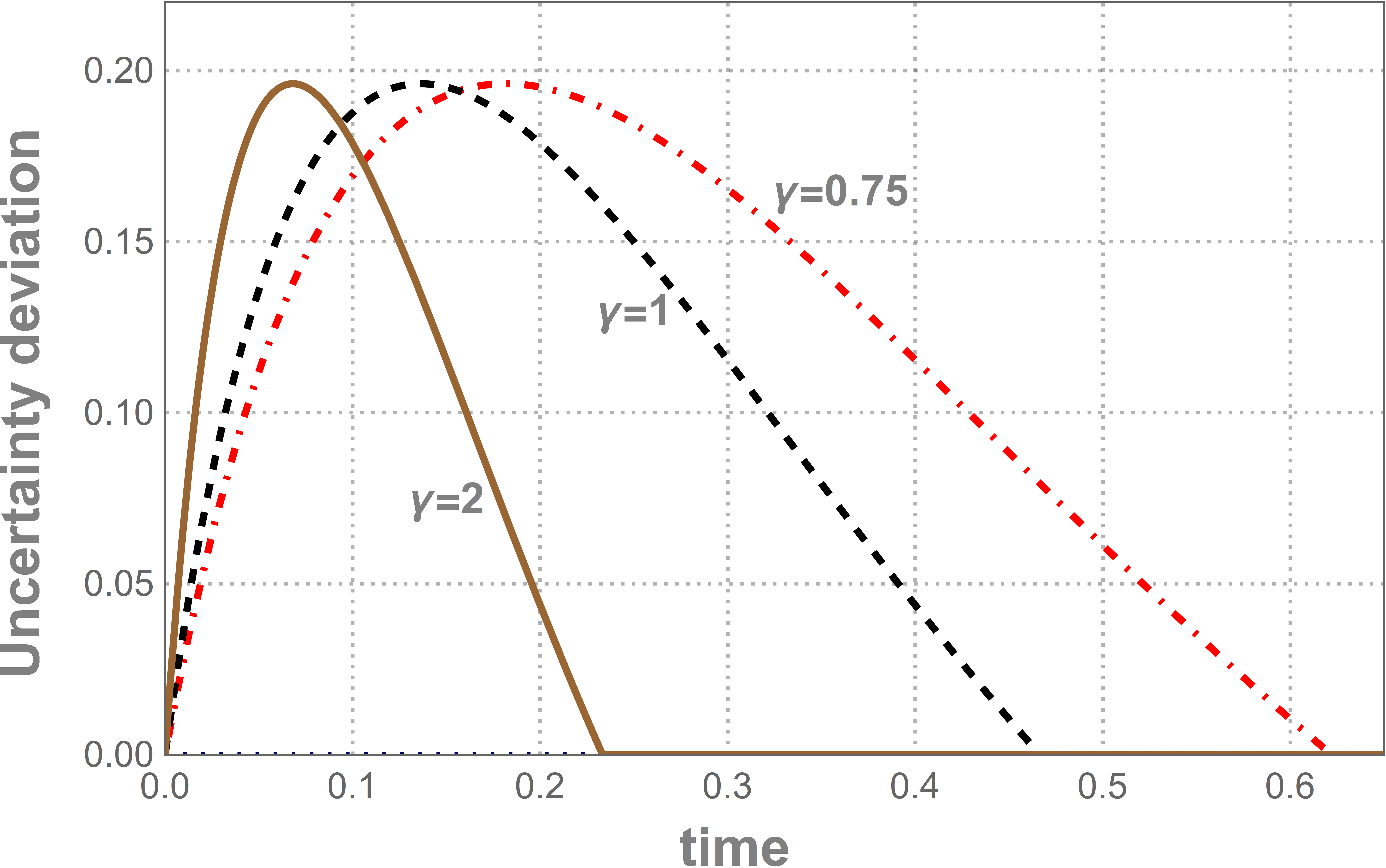
Figure 2: In this plot we verify the QSI in Eq. (15) for the stated qubit dynamics. The uncertainty deviation i.e, the difference between the left-hand side (LHS) and the right-hand side (RHS) of Eq. (15) for $\rho=\ket{1}\bra{1}$ for different values of $\gamma$ are plotted. The difference [$=\Delta\mathcal{I}_{S}(\rho(t))+\mathcal{Q}_{S}(t)-\Delta\mathcal{I}_{\epsilon}(\rho(t))$] increases initially but comes down to zero to settle there. As expected from the inequality relation, it is never negative.

IV.3 QSI for noisy quantum switches

We consider two different ways noise can be introduced to the QS. In the first case, the noise is quantum while in the second case, the noise is classical. By quantum noise, we mean that for the control qubit, an arbitrary pure state is used instead of the $\ket{+}$ state and for the measurement, another arbitrary pure state is used in the place of $\ket{+}\bra{+}$. For the case of the classical noise, we consider a mixed state in the $\ket{\pm}$ basis as the control and an arbitrary positive operator-valued measure (POVM) on the same basis. Before getting into the study, it is necessary to understand whether the QSI is valid for these general situations. For that, we need to verify Statement 1 for such a generalised QS evolution. In Appendix C, we prove it for such a general consideration with an arbitrary control qubit and final measurement. We show that for the generalised Pauli channel, the fixed point remains unchanged under the QS operation. This is the only prerequisite for the validity of Eqs. (15) and (18) and hence it asserts that QSI is perfectly legible for the following considerations.

IV.3.1 Quantum noise

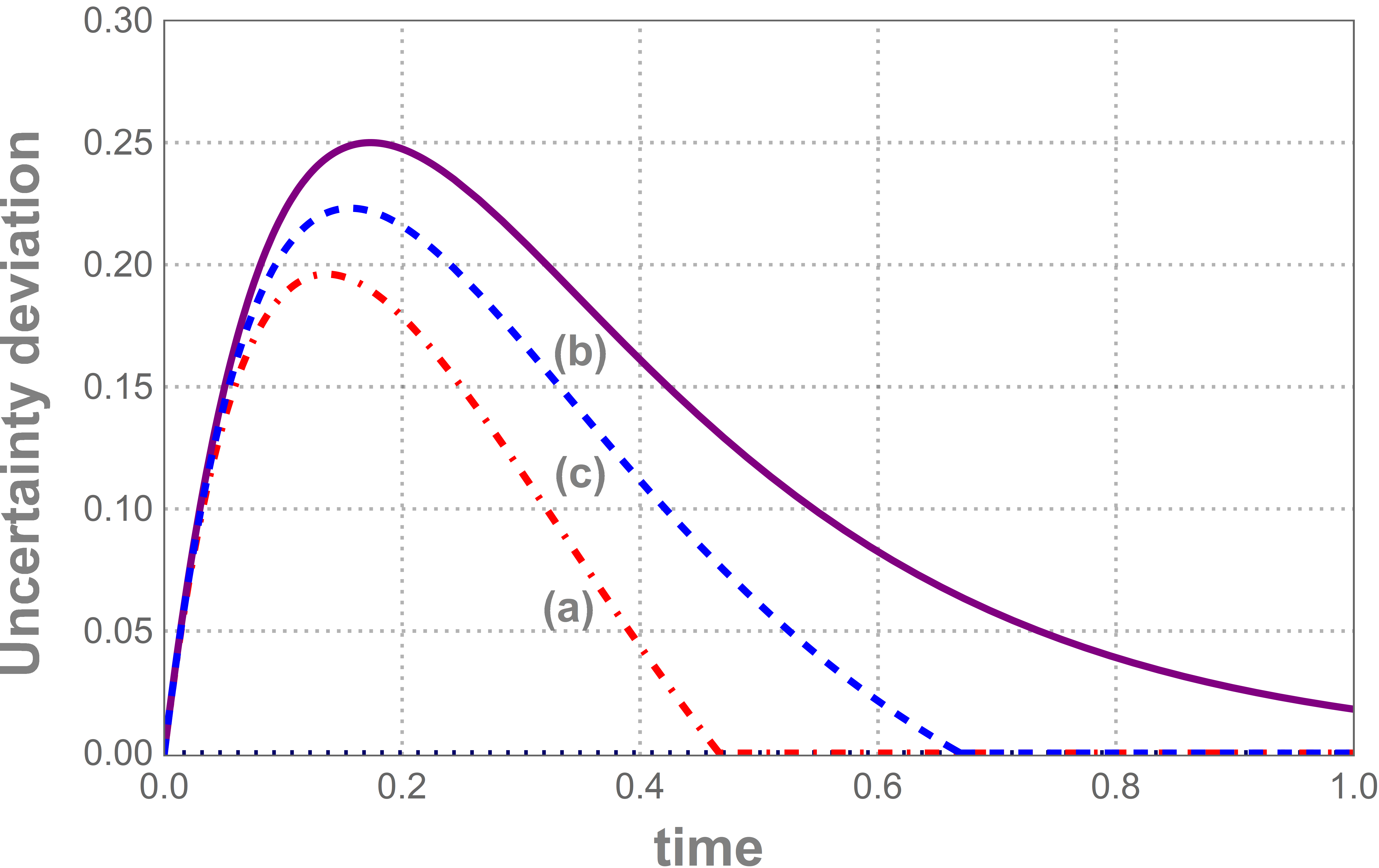
Figure 3: Here we depict the QSI for a noisy QS described in Section IV.3.1. The difference between the left and right-hand sides of Eq. (15) for $\rho=\ket{1}\bra{1}$ and $\gamma=1$. For $\{p,\ q\}\ =$ (a) $\{1/2,\ 1/2\}$, (b) $\{2/5,\ 1\}$, and (c) $\{4/5,\ 9/10\}$

.

The control qubit is prepared in the state, $\omega_{c}=\sqrt{p}|0\rangle+\sqrt{(1-p)}|1\rangle$ and the measurement on the control system is performed in the $\{\ket{\mathcal{M}_{q}}\bra{\mathcal{M}_{q}},\mathbb{I}-\ket{\mathcal{M}_{q}}\bra{\mathcal{M}_{q}}\}$ basis with $\ket{\mathcal{M}_{q}}=\sqrt{q}|0\rangle+\sqrt{(1-q)}|1\rangle$, with $p,~{}q$ being arbitrary probabilities. After the measurement, the state of the generic target system corresponding to the ${}^{\prime}+^{\prime}$ outcome becomes

$$\Phi^{S}_{t}(\rho)=\frac{1}{\mathcal{A}_{2}}{}_{c}\left\langle\mathcal{M}_{q}\left|S(\rho\otimes\omega_{c})\right|\mathcal{M}_{q}\right\rangle_{c}$$

$$=\left(\begin{array}[]{cc}A_{pq}(t)\rho_{11}(0)+B_{pq}(t)\rho_{22}(0)&C_{pq}(t)\rho_{12}(0)\\ C_{pq}(t)\rho_{21}&B_{pq}(t)\rho_{11}(0)+A_{pq}(t)\rho_{22}(0)\end{array}\right)$$ (41)

with $A_{pq}(t)=(1+C_{pq}(t))/2$, $B_{pq}(t)=(1-C_{pq}(t))/2$, and

$$C_{pq}(t)=\frac{f_{p}f_{q}(\mathcal{G}^{2}-2\mathcal{G}+5)+p(4q-2)+2(1-q)}{f_{p}f_{q}(\mathcal{G}^{2}+6\mathcal{G}-3)+p(4q-2)\mathcal{G}^{2}}$$

where $f_{x}=\sqrt{x(1-x)}$ and $\mathcal{A}_{2}$ is the normalisation factor.

Fig. 3 confirms that the QSI is valid in this case, however, it takes more time to reach the equality with the varying noise parameter.

IV.3.2 Classical noise

We can now consider the case where the control qubit is prepared in the Fourier basis as, $\omega_{c}=p|+\rangle_{c}\langle+|+(1-p)|-\rangle_{c}\langle-|$ and the measurement on the control qubit is performed in the POVM set, $\{\mathcal{M}_{q_{1},q_{2}},\mathbb{I}-\mathcal{M}_{q_{1},q_{2}}\}$ where $\mathcal{M}_{q_{1},q_{2}}=q_{1}|+\rangle_{c}\langle+|+q_{2}|-\rangle_{c}\langle-|$. The final state of the target system after the measurement is performed on the above basis would be given by:

$$\Phi^{S}_{t}(\rho)=\frac{1}{\mathcal{A}_{3}}{\rm Tr}_{c}\left(\mathcal{M}_{q_{1},q_{2}}S(\rho\otimes\omega_{c})\right)=$$

$$\small\left(\begin{array}[]{cc}A_{pq_{1}q_{2}}(t)\rho_{11}(0)+B_{pq_{1}q_{2}}(t)\rho_{22}(0)&C_{pq_{1}q_{2}}(t)\rho_{12}(0)\\ C_{pq_{1}q_{2}}(t)\rho_{21}&B_{pq_{1}q_{2}}(t)\rho_{11}(0)+A_{pq_{1}q_{2}}(t)\rho_{22}(0)\end{array}\right)$$ (44)

with $A_{pq_{1}q_{2}}(t)=\left(1+C_{pq_{1}q_{2}}(t)\right)/2$, $B_{pq_{1}q_{2}}(t)=\left(1-C_{pq_{1}q_{2}}(t)\right)/2$, and

$$C_{pq_{1}q_{2}}(t)=\frac{(-1+10p+\mathcal{G}^{2}(-1+2p)+\mathcal{G}(2-4p))q_{1}-(-9+10p+\mathcal{G}^{2}(-1+2p)+\mathcal{G}(2-4p))q_{2}}{(3-6p+\mathcal{G}^{2}(3+2p)+6\mathcal{G}(-1+2p))q_{1}-(3-6p+\mathcal{G}^{2}(-5+2p)+\mathcal{G}(-1+2p))q_{2}},$$

where $\mathcal{A}_{3}$ is the normalisation factor.

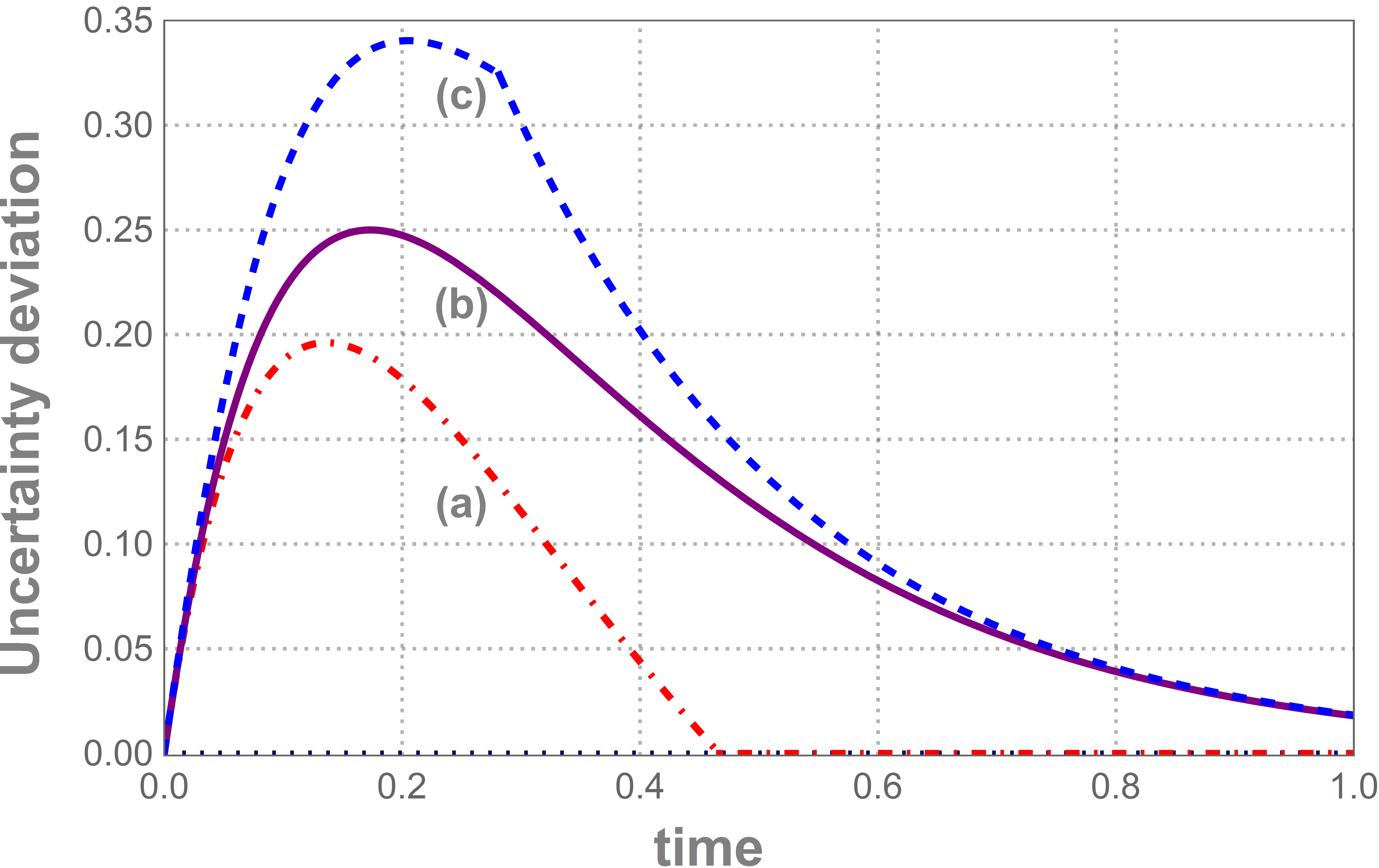
Figure 4: Here we depict the uncertainty deviation for the “classical noise case" for $\rho=\ket{1}\bra{1}$, with $\{p,\ q_{1},q_{2}\}\ =$ (a) $\{1,\ 1,\ 0\}$, (b) $\{1/2,\ 1/2,\ 1/2\}$, and (c) $\{4/5,\ 1/10,\ 9/10\}$

.

Fig. 4 confirms the validity of QSI for this noisy QS, though, similar to the case of quantum noise, it takes more time to reach the equilibrium with the addition of noise.

V Lindblad dynamics of the switched channel

We are now in a position to derive the canonical Lindblad-type master equation for the dynamical map generated under the action of the QS. It is important to note that after the switching action, when the control bit is finally measured, we consider the dynamics of only one outcome (‘$+$’) even though both outcomes (‘$+$’,‘$-$’) are possible. Therefore, it may seem that after normalising, the operation may not be linear anymore, and hence deriving the Lindblad equation is not possible. However, in our case, the trace of the final state density matrix [Eq. (IV.2)] is independent of the initial state (since $A(t)+B(t)=1$) and thus, the linearity is left intact. In particular, we prove that for any generalized Pauli channel represented by Eq. (6), the final map after post-selection is independent of the initial state.

$\blacksquare$ Statement 2: For any generalised Pauli channel, the final map obtained after post-selection and the switch action presented in Eq. (IV.2) is linear.

Proof.

Using the properties of the Weyl operators, we can show that

$$\text{Tr}\left[\rho\sum_{k,l,r,s}\widetilde{W}_{klrs}^{\dagger}\widetilde{W}_{klrs}\right]= \ \text{Tr}\left[\rho\sum_{k,l,r,s}\frac{p_{kl}p_{rs}}{2}(1+\omega^{ks-rl})\mathbb{I}\right]$$

$$= \ \sum_{k,l,r,s}\frac{p_{kl}p_{rs}}{2}(1+\omega^{ks-rl}).$$ (45)

This shows that the trace is independent of the input density matrix and hence the linearity is preserved. ∎

In Appendix D, we briefly sketch the method to obtain the Lindblad operator for a dynamical map. Applying it on Eq. (IV.2), we get the corresponding Lindblad-type master equation of the form

$$\frac{d}{dt}\rho(t)=\Gamma_{S}(t)\sum_{i=1}^{3}\left(\sigma_{i}.\rho(t).\sigma_{i}-\rho(t)\right),$$ (46)

with

$$\Gamma_{S}(t)=\ \ \ 8\gamma \ \times\ \frac{\cosh(4\gamma t)-2\sinh(4\gamma t)+3}{5\cosh(4\gamma t)-4\sinh(4\gamma t)-1}$$

$$\ \times\ \frac{1}{4\sinh(4\gamma t)+\cosh(4\gamma t)+3}$$

$$=\ 16\gamma \ \times\ \frac{(-\mathcal{G})(\mathcal{G}^{2}-6\mathcal{G}-3)}{(\mathcal{G}^{2}-2\mathcal{G}+9)(5\mathcal{G}^{2}+6\mathcal{G}-3)}$$ (47)

The above coefficient becomes negative with time as shown in Fig. 5. This implies the QS has converted the initial Markovian operation (i.e., the completely depolarising channel) into a non-Markovian one.

V.1 Emergent non-Markovianity from the quantum switch

We further explore various aspects of non-Markovianity (Breuer et al., 2004; Laine et al., 2010; Rivas et al., 2010, 2014; Vasile et al., 2011; Lu et al., 2010; Luo et al., 2012; Fanchini, 2014; Chanda and Bhattacharya, 2016; Haseli, 2014; Mukhopadhyay et al., 2017; Bhattacharya et al., 2020a, b; Maity et al., 2020; Bhattacharya and Bhattacharya, 2021; Bhattacharya et al., 2018; Das et al., 2021) emerging from the QS dynamics. Quantum non-Markovianity can be measured in several ways. One such measure is based on the divisibility of a dynamical map which was first proposed by Rivas, Huelga and Plenio (RHP) Rivas et al. (2010).

RHP measure: The dynamical map $\Phi_{\Delta t}\equiv\Phi(t+\Delta t,t)$ is CP if and only if $(\mathbb{I}\otimes\Phi_{\Delta t})\ket{\psi}\bra{\psi}\geq 0$ for all $\Delta t$ Rivas et al. (2010), where $\mathbb{I}$ stands for the identity map. Utilizing the trace-preserving condition, we can use the identity $||(\mathbb{I}\otimes\Phi_{\Delta t})\ket{\psi}\bra{\psi}||_{1}=1$ if and only if $\Phi_{\Delta t}$ is CP; otherwise $||(\mathbb{I}\otimes\Phi_{\Delta t})\ket{\psi}\bra{\psi}||_{1}>1$. Using this property, the RHP measure is defined as

$$g(t)=\lim_{\Delta t\rightarrow 0}\frac{||\mathbb{I}\otimes\Phi_{\Delta t}\ket{\psi}\bra{\psi}||_{1}-1}{\Delta t},$$ (48)

where $\Phi_{\Delta t}=\mathbb{I}+\Delta t{\mathcal{L}}_{t}$. The integral $\int_{0}^{\infty}g(t)dt$ can be considered as a measure of non-Markovianity. For the switch operation, it is straightforward to calculate that $g(t)=6|\Gamma_{S}(t)|$. Therefore, from the perspective of the divisibility of dynamical maps, we can measure the QS-induced non-Markovianity with

$$N_{S}=\int_{T_{-}}^{\infty}g(t)dt=\int_{T_{-}}^{\infty}6|\Gamma_{S}(t)|dt,$$ (49)

or the normalised measure,

$$\mathcal{N}_{S}=\frac{N_{S}}{1+N_{S}}.$$ (50)

In Fig. 5(a), the RHP measure of non-Markovianity is depicted with different values of $\gamma$. It clearly shows the time dependence of the emergent non-Markovianity due to the QS.

BLP measure: Another well-known measure of non-Markovianity was proposed by Breuer, Laine, and Piilo (BLP) Breuer et al. (2009); Laine et al. (2010). They characterised non-Markovian dynamics by the information backflow from the environment to the system. Usually, the distinguishability between two states decreases under Markovian dynamics as information moves from the system to the environment. Thus, an increase in the distinguishability of a pair of evolving states indicates information backflow under the dynamics. According to the BLP measure, a dynamics is non-Markovian if there exist a pair of states whose distinguishability increases for some time $t$. The time derivative of the distance between two states $\rho$ and $\tau$ evolving under the QS is given as

$$\mathcal{B}\equiv\frac{d}{dt}D(\Phi^{S}_{t}(\rho),\tau).$$ (51)

The BLP measure of non-Markovianity is calculated by integrating $\mathcal{B}$ over the time where $\mathcal{B}>0$,

$$N_{\rm inf}=\int_{T_{-}}^{\infty}\mathcal{B}dt=D(\Phi^{S}_{\infty}(\rho),\tau)-D(\Phi^{S}_{T_{-}}(\rho),\tau).$$ (52)

From Definition 3 [Eq. (14)], we can calculate QSM for $t\rightarrow\infty$:

$$\mathcal{Q}_{S}(\infty)=D({\Phi}^{S}_{\infty}(\rho),\tau)=N_{\rm inf}+D({\Phi}^{S}_{T_{-}}(\rho),\tau).$$ (53)

This establishes the direct connection between the emergent non-Marvonianity and the QSM—the QSM is the emergent non-Markovianity up to a scaling factor. Moreover, we can consider the normalised BLP measure,

$$\mathcal{N}_{\rm BLP}=\frac{N_{\rm inf}}{1+N_{\rm inf}},$$ (54)

to get

$$\mathcal{Q}_{S}(\infty)=\frac{\mathcal{N}_{\rm BLP}}{1-\mathcal{N}_{\rm BLP}}+D({\Phi}^{S}_{T_{-}}(\rho),\tau).$$ (55)

We can also consider a normalised QSM measure:

$$\mathcal{N}_{S}^{\infty}=\frac{\mathcal{Q}_{S}(\infty)}{1+\mathcal{Q}_{S}(\infty)},$$ (56)

which gives us the following relation,

$$\mathcal{N}_{S}^{\infty}=\frac{\mathcal{N}_{\rm BLP}+D({\Phi}^{S}_{T_{-}}(\rho),\tau)(1-\mathcal{N}_{\rm BLP})}{1+D({\Phi}^{S}_{T_{-}}(\rho),\tau)(1-\mathcal{N}_{\rm BLP})}.$$ (57)

For highly non-Markovian cases, when $\mathcal{N}_{\rm BLP}\rightarrow 1$, we have $\mathcal{N}_{S}^{\infty}\rightarrow\mathcal{N}_{\rm BLP}$.

In Fig. 5(b), the BLP measure of non-Markovianity is shown for different values of $\gamma$, which shows the evolution of information backflow of the emergent non-Markovian dynamics with time. From Fig. 5, it is evident that, at a certain characteristic time, there is a clear transition from Markovian to non-Markovian behaviour for the concerned dynamics. Below, we analyse this particular issue.

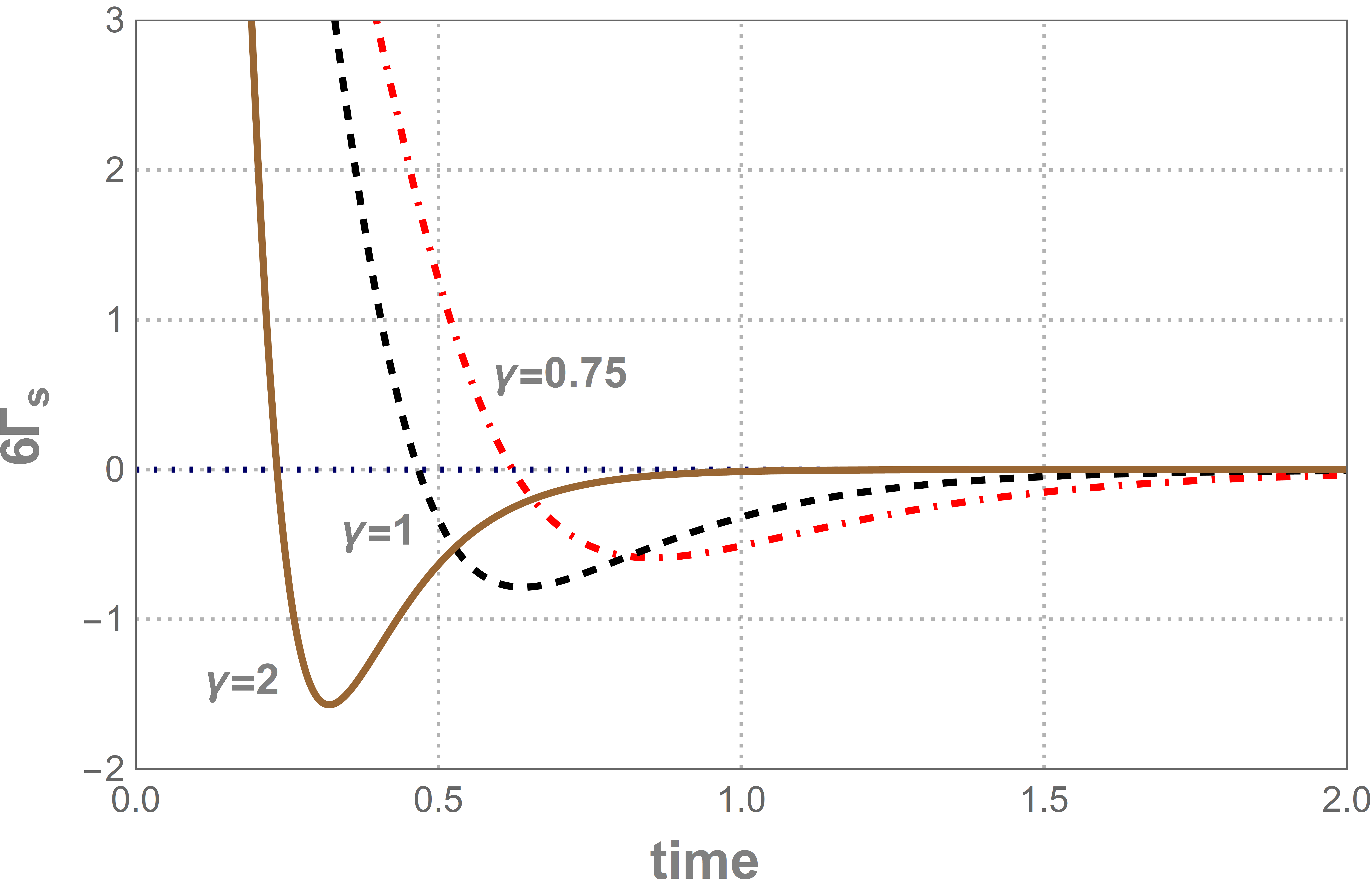
((a)) (a)

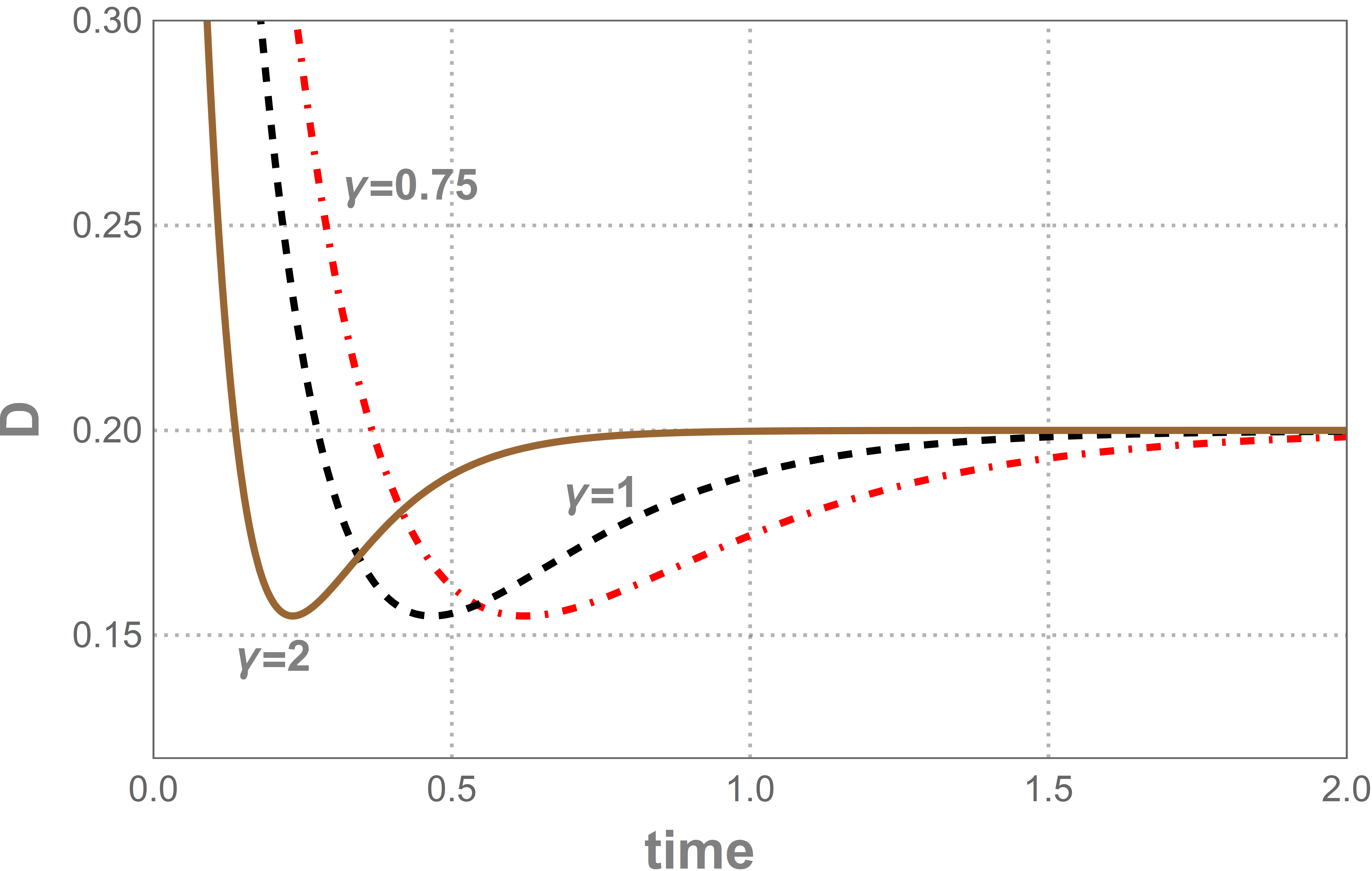
((b))    (b)

Figure 5: Here, we represent the evolution of RHP and BLP measure for the given qubit dynamics, for three different values of $\gamma$ as mentioned in the plot. It depicts the emergent non-Markovianity due to the action of QS. It also shows that the information backflow (plot (b)) emerges at the same time when divisibility of the channel breaks down (plot (a))

V.2 Characteristic time

Let $T_{-}$ be the characteristic time— the earliest time when information backflow starts. This is the time when the Lindblad coefficient in Fig. 5 turns negative; below, we show this explicitly. Let us consider two arbitrary states,

$$\chi_{i}(t)=\frac{1}{2}(\mathbb{I}+\vec{\sigma}\cdot\vec{n}_{i}(t))$$ (58)

with $i=1,2$, and $\vec{n}_{i}(t)=\{n_{i}^{1}(t),n_{i}^{2}(t),n_{i}^{3}(t)\}$. The trace distance between these two states can be written as

$$D\left(\chi_{1}(t),\chi_{2}(t)\right)=\sqrt{(a_{1}(t))^{2}+(a_{2}(t))^{2}+(a_{3}(t))^{2}},$$ (59)

where $a_{k}(t)=n_{1}^{k}(t)-n_{2}^{k}(t)$. Since, at $t=T_{-}$, the trace distance attains an extremum value, its time derivative vanishes, i.e.,

$$\frac{d}{dt}D\left(\chi_{1}(T_{-}),\chi_{2}(T_{-})\right)=0.$$ (60)

After simplification, this condition reduces to

$$\lim_{\epsilon\to 0}\;\sum_{i=1}^{3}\left[(a_{i}(T_{-}+\epsilon))^{2}-(a_{i}(T_{-}))^{2}\right]=0.$$ (61)

Expanding, we get $a_{i}(T_{-}+\epsilon)=a_{i}(T_{-})(1+\epsilon\Gamma_{s}(T_{-}))$. This implies, $((a_{1}(T_{-}))^{2}+(a_{2}(T_{-}))^{2}+(a_{3}(T_{-}))^{2})\Gamma_{s}(T_{-})=0$. Clearly, the time derivative of the trace distance becomes zero and then positive, exactly when $\Gamma_{s}(t)$ becomes zero and then negative. Therefore, the characteristic time $T_{-}$ can be evaluated from the equation $\Gamma_{s}(T_{-})=0$. We thus get

$$\cosh(4\gamma T_{-})-2\sinh(4\gamma T_{-})+3=0$$

$${\rm or,}\quad \mathcal{G}_{-}^{2}-6\mathcal{G}_{-}-3=0,~{}~{}\mbox{with}~{}~{}\mathcal{G}_{-}=e^{4\gamma T_{-}}.$$ (62)

Solving this, we obtain the expression of characteristic time as,

$$T_{-}=\frac{1}{4\gamma}\ln\left(2\sqrt{3}+3\right).$$ (63)

In the literature of quantum non-Markovianity, the system-environment correlation is considered as one of the primary reasons behind the generation of non-Markovian dynamics. In the case of the QS, the control qubit can be interpreted as a part of the environment and the QSM can be understood as the emergent non-Markovianity. Here it is important to remember that CP-divisible operations are not convex. Therefore for two such operations, $\Phi_{1}$ and $\Phi_{2}$, the operation $p\Phi_{1}\circ\Phi_{2}+(1-p)\Phi_{2}\circ\Phi_{1}$ may not be CP divisible. One may question the usefulness of the QS for the emergence of non-Markovianity, as discussed previously. Indeed, if one uses two different CP-divisible operations, the QS is not unique in generating non-Markovian dynamics that can be called a “self-switching process”. However, if one uses the same operations as $\Phi_{1}=\Phi_{2}=\Phi$, neither convex combination nor any series or parallel combinations of those operations can produce non-Markovian dynamics, except the QS.

Finally, we study the emergent non-Markovianity due to the QS for a general qubit Pauli channel given in Eq. (20) with constant but different Lindblad coefficients, in terms of the normalised RHP measure $\mathcal{N}_{S}$. The result is shown in Fig. 6 for multiple Lindblad coefficients. The figure shows that by manipulating the coefficients, we can produce highly non-Markovian dynamics, starting from a purely Markovian depolarising evolution.

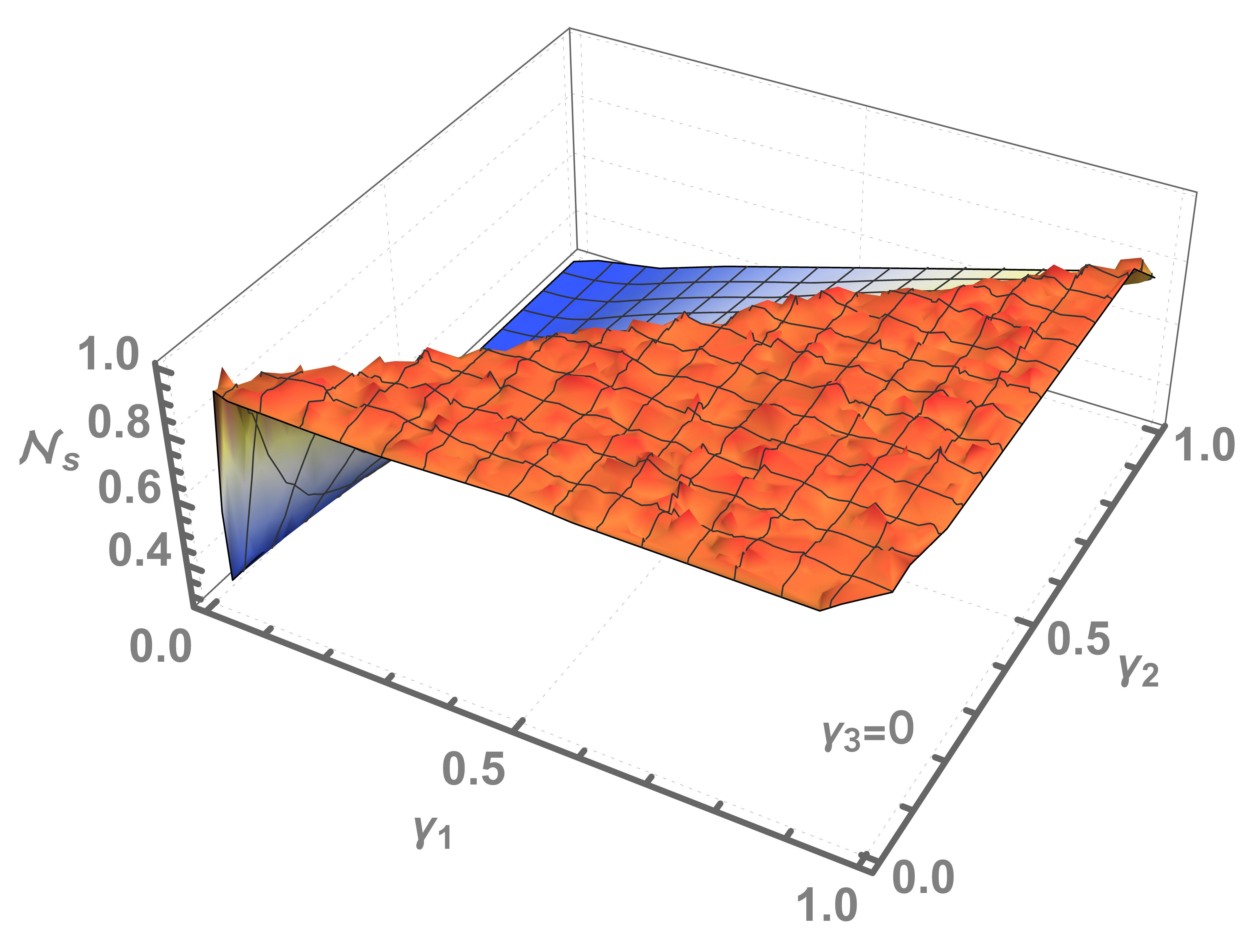
((a)) (a)

((b))

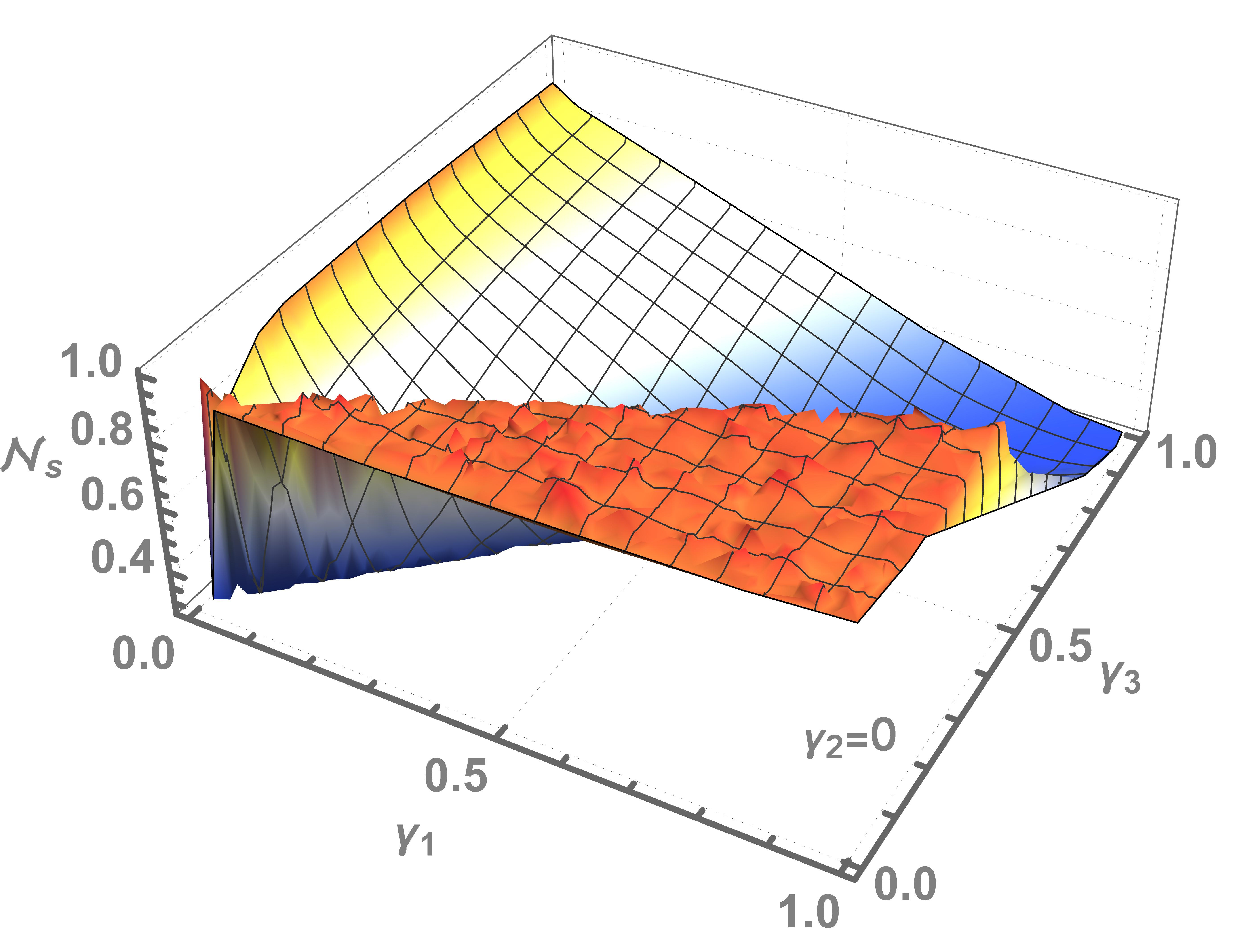
((c))    (b)

Figure 6: In this plot, we show the emergent non-Markovianity in terms of $\mathcal{N}_{S}$ for QS action over a general Pauli channel given in Eq. (20) with different Lindblad coefficients. In case (a) we consider $\gamma_{3}=0$ and vary $\gamma_{1}$ and $\gamma_{2}$ from 0 to 1. We see that for high values of them, the QS channel is highly non-Markovian. In case (b), we see similar features for $\gamma_{2}=0$.

VI Discussion

A series of recent works establish the advantages arising from the superposition of alternative causal orders over the superposition of alternative trajectories. Although, recent debates suggest that the advantages appearing due to the superposition of causal order can be achieved and even be surpassed by the superposition of direct pure process with definite order Guerin et al. (2019), however, proper characterization and adequate quantification of indefinite causal order are still not well understood. With this motivation, in this paper, we explore the dynamical behaviour of the QS and characterise the non-Markovian memory that emerges from it. We first investigate how the loss of information of a general quantum evolution changes when it is subjected to the QS and, on this backdrop, we propose a quantification of the switch-induced memory, QSM. We then derive an uncertainty relation between the information loss and the QSM, which captures the interplay between information storage capacity and the QSM. Furthermore, we show that after a sufficiently long period of time, as the dynamics approaches the steady state, the uncertainty inequality reduces to an equality, implying a complementarity between the long-time averaged loss of information and the QSM. We then consider an example of completely depolarizing dynamics for qubit and explore its behaviour under the action of QS. We make both the control qubit and the final measurement on the control qubit noisy and look at the amount of noise that a quantum switch can tolerate. Further, we derive the reduced operation of the switch action on the qubit both in terms of the Kraus representation and Lindblad evolution and verify the uncertainty relation in this particular case. We then attribute this effect of the QS for activating a completely depolarizing channel to the non-Markovian memory that emerges from the switch-induced memory. Comparing it with other standard measures of non-Markovianity, we show that the long-term memory of a QS is equivalent to the emergent non-Markovianity.

Our work is particularly relevant from several backdrops of quantum information theory. While investigating the dynamical behaviour of a quantum switch, we find that the quantum switch actually carries some non-Markovian memory. The emergence of such non-Markovian memory induced by the quantum switch is quite important for further developments of quantum technology and near-term quantum devices. Furthermore, this investigation also allows us to quantify the amount of memory a quantum switch can possess. In other words, our study opens up a new avenue for quantifying the amount of noise a quantum switch can tolerate. To the best of our knowledge, this is the first study for adequate quantification of the quantum switch, a well-established quantum resource for future quantum technologies.

Appendix A Calculation of the time-averaged state of the dynamical map

As mentioned earlier, for a completely depolarizing channel, the dynamical map is given by the following equations:

$$\rho_{11}(t)= \ \rho_{11}(0)\left(\frac{1+e^{-2\xi_{1}(t)}}{2}\right)+\rho_{22}(0)\left(\frac{1-e^{-2\xi_{1}(t)}}{2}\right),$$

$$\rho_{22}(t)= \ 1-\rho_{11}(t),$$

$$\rho_{12}(t)= \ \rho_{12}(0)e^{-\xi_{2}(t)},$$

with

$$\xi_{1}(t)= \ \int_{0}^{t}\left[\gamma_{1}(s)+\gamma_{2}(s)\right]ds\quad\text{and}$$

$$\xi_{2}(t)= \ \int_{0}^{t}\left[\gamma_{2}(s)+\gamma_{3}(s)\right]ds.$$

Now the time-averaged state for the above dynamics is given by

$$\overline{\rho} =\lim_{T\to\infty}\frac{\int_{0}^{T}\Phi_{t}(\rho)\,dt}{\int_{0}^{T}dt}$$

$$=\lim_{T\to\infty}\frac{\bigints_{0}^{T}\left(\begin{array}[]{ll}\rho_{11}(t)&\rho_{12}(t)\\ \rho_{21}(t)&\rho_{22}(t)\end{array}\right)\,dt}{\int_{0}^{T}dt} =\left(\begin{array}[]{ll}\frac{1}{2}&0\\ 0&\frac{1}{2}\end{array}\right) =\frac{\mathbb{I}}{2}.$$

If $\tau$ is a fixed point of the dynamical map $\Phi$, then

$$\mathcal{L}_{t}(\tau) =\sum_{i=0}^{3}\gamma_{i}\left[\sigma_{i}\tau\sigma_{i}-\tau\right]=0.$$

Solving the above equations, we get

$$\tau=\left(\begin{array}[]{ll}\frac{1}{2}&0\\ 0&\frac{1}{2}\end{array}\right)=\frac{\mathbb{I}}{2}.$$

This shows that the ergodicity condition is satisfied.

Appendix B Kraus representation of the quantum switch

The evolution of the combined state of the target system and the control qubit under the switch is given by

$$S\left(\mathcal{E},\mathcal{E}\right)\left(\rho\otimes\omega_{c}\right)=\sum_{i,j}S_{ij}\left(\rho\otimes\omega_{c}\right)S_{ij}^{\dagger}$$

The state of the target system after measuring the control qubit in the $\left\{|\pm\rangle_{c}\langle\pm|\right\}$ basis is given by ${}_{c}\left\langle+\left|S\left(\mathcal{E},\mathcal{E}\right)\left(\rho\otimes|+\rangle_{c}\langle+|\right)\right|+\right\rangle_{c}$. This can also be written as

$$\sum_{i,j}M_{ij}\rho M_{ij}^{\dagger}$$

with

$$M_{ij}=\frac{K_{i}K_{j}+K_{j}K_{i}}{2}$$

and $\sum_{i,j}M_{ij}^{\dagger}M_{ij}\leq\mathbb{I}$. The equality holds if $[K_{i},K_{j}]=0$ or $[K_{i},K_{j}^{\dagger}]=0$ or both. Therefore, the switch action

$$\Phi^{S}_{t}(\rho)=\frac{\sum_{i,j}M_{ij}\rho M_{ij}^{\dagger}}{\text{Tr}\left[\rho\sum_{i,j}M_{ij}^{\dagger}M_{ij}\right]}$$

Now, this operation is CPTP, but the linearity is only confirmed if $\text{Tr}\left[\rho\sum_{i,j}M_{ij}^{\dagger}M_{ij}\right]$ is independent of $\rho$. For our case it is independent of $\rho$, so linearity is confirmed.

Appendix C Proof of Statements 1 and 2 for the control qubit in the superposition state and measurement with a parameter

Here we will prove Statement 1 and Statement 2 for a general switch operation which includes all the cases discussed in Sections III, IV, and V. A general quantum switch operation can be represented by

$$\Phi_{t}^{S}(\rho)=\frac{1}{\mathcal{P}}Tr_{c}\left[M_{\alpha}\left(\sum_{ij}W_{ij}\rho\otimes\omega_{c}W_{ij}^{\dagger}\right)\right],$$

with $\omega_{c}=\sum_{\kappa}q_{\kappa}\ket{\psi_{\kappa}}\bra{\psi_{\kappa}}$ being a general qubit control state, $M_{\alpha}=A_{\alpha}^{\dagger}A_{\alpha}$ being a general Positive operator valued measure, $\mathcal{P}$ being the normalisation factor, $W_{ij}=K_{i}K_{j}\otimes\ket{0}\bra{0}+K_{j}K_{i}\otimes\ket{1}\bra{1}$ where $K_{i}$s are the Kraus operators for the original quantum operation and $Tr_{c}[~{}~{}]$ representing partial trace over the control basis. For this setting, the reduced Kraus representation can be expressed as

$$\tilde{K}_{ij}=\chi_{1}K_{i}K_{j}+\chi_{2}K_{j}K_{i},$$

with $\chi_{1}=\sum_{l,\kappa}\sqrt{q_{\kappa}}\bra{\psi_{l}}A_{\alpha}\ket{0}\langle 0|\psi_{\kappa}\rangle$ and $\chi_{2}=\sum_{l,\kappa}\sqrt{q_{\kappa}}\bra{\psi_{l}}A_{\alpha}\ket{1}\langle 1|\psi_{\kappa}\rangle$. Therefore the switch operation can be represented as

$$\Phi_{t}^{S}(\rho)=\frac{1}{\mathcal{P}}\sum_{ij}\tilde{K}_{ij}\rho\tilde{K}^{\dagger}_{ij},$$

with $\mathcal{P}=Tr\left[\sum_{ij}\tilde{K}_{ij}\rho\tilde{K}^{\dagger}_{ij}\right]$. Using this general representation for arbitrary dimensional depolarising operations represented in Eq. (6) and following the same method, we can prove Statement 1 and Statement 2 for such general switch actions. It is to be noted that the dynamical maps constructed in Eqs. (IV.2), (IV.3.1), and (IV.3.2) are all special cases of the general form discussed in this appendix.

Appendix D Construction of the master equation

Let us now consider a dynamical map of the form

$$\rho(t)=\Omega[\rho(0)].$$ (64)

Further, consider the equation of motion corresponding to the previous dynamical equation to be

$$\dot{\rho}(t)=\tilde{\Lambda}[\rho(t)]$$ (65)

where $\tilde{\Lambda}[.]$ is the generator of the dynamics. Now following Ref. Hall et al. (2014); Bhattacharya et al. (2017), we can find the master equation and generator of the dynamics.

Let $\{\mathcal{G}_{i}\}$ denotes the orthonormal basis set with the properties $\mathcal{G}_{0}=\mathbb{I}/\sqrt{2}$, $\mathcal{G}_{i}^{\dagger}=\mathcal{G}_{i}$, $\mathcal{G}_{i}$ are traceless except $\mathcal{G}_{0}$ and $\text{Tr}[\mathcal{G}_{i}\mathcal{G}_{j}]=\delta_{ij}$. The map in Eq. (64) can be represented as

$$\Omega[\rho(0)]=\sum_{m,n}\text{Tr}[\mathcal{G}_{m}\Omega[\mathcal{G}_{n}]]\text{Tr}[\mathcal{G}_{n}\rho(0)]\mathcal{G}_{m}=[F(t)r(0)]\mathcal{G}^{T}$$

where $F_{mn}=\text{Tr}[\mathcal{G}_{m}\Omega[\mathcal{G}_{n}]]$ and $r_{n}(s)=\text{Tr}[\mathcal{G}_{n}\rho(s)]$. Taking time-derivative of the above equation we shall get

$$\dot{\rho}(t)=[\dot{F}(t)r(0)]\mathcal{G}^{T}.$$

Let us now consider a matrix $L$ with elements $L_{mn}=\text{Tr}[\mathcal{G}_{m}\tilde{\Lambda}[\mathcal{G}_{n}]]$. We can therefore represent Eq. (65) as

$$\dot{\rho}(t)=\sum_{m,n}\text{Tr}[\mathcal{G}_{m}]\tilde{\Lambda}[\mathcal{G}_{n}]\text{Tr}[\mathcal{G}_{n}\rho(t)]\mathcal{G}_{m}=[L(t)r(t)]\mathcal{G}^{T}.$$

Comparing the above two equations, we find

$$\dot{F}(t)=L(t)F(t)\implies L(t)=\dot{F}(t)F(t)^{-1}.$$

One may note that $L(t)$ can be obtained if $F(t)^{-1}$ exists and $F(0)=\mathbb{I}$. From this $L(t)$ matrix, we can derive the corresponding master equation following the methods given in Refs. Hall et al. (2014); Bhattacharya et al. (2017). It is to be noted that of the dynamical maps constructed in Eqs. (IV.2), (IV.3.1), and (IV.3.2), all have the following form

$$\begin{array}[]{ll}\rho_{11}(t)=\left(\frac{1+\mathcal{C}(t)}{2}\right)\rho_{11}(0)+\left(\frac{1-\mathcal{C}(t)}{2}\right)\rho_{22}(0),\\ \\ \rho_{22}(t)=\left(\frac{1-\mathcal{C}(t)}{2}\right)\rho_{11}(0)+\left(\frac{1+\mathcal{C}(t)}{2}\right)\rho_{22}(0),\\ \\ \rho_{12}(t)=\mathcal{C}(t)\rho_{12}(0),~{}~{}\rho_{21}(t)=\rho_{12}^{*}(t),\end{array}$$ (66)

where $\mathcal{C}(t)$ is a real function of time. For these evolutions, the $L(t)$ matrices will be of the form

$$L(t)=\left(\begin{matrix}0&0&0&0\\ 0&\frac{d}{dt}\ln\mathcal{C}(t)&0&0\\ 0&0&\frac{d}{dt}\ln\mathcal{C}(t)&0\\ 0&0&0&\frac{d}{dt}\ln\mathcal{C}(t)\end{matrix}\right).$$ (67)

The corresponding master equation will be of the form

$$\frac{d}{dt}\rho(t)=\Gamma_{\mathcal{C}}(t)\sum_{i}\left[\sigma_{i}\rho(t)\sigma_{i}-\rho(t)\right],$$ (68)

with

$$\Gamma_{\mathcal{C}}(t)=-\frac{1}{4}\frac{d}{dt}\ln\mathcal{C}(t).$$

References

- Gisin et al. (2005) N. Gisin, N. Linden, S. Massar, and S. Popescu, “Error filtration and entanglement purification for quantum communication,” Phys. Rev. A 72, 012338 (2005).
- Chiribella et al. (2013) G. Chiribella, G. M. D’Ariano, P. Perinotti, and B. Valiron, “Quantum computations without definite causal structure,” Phys. Rev. A 88, 022318 (2013).
- Chiribella (2012) G. Chiribella, “Perfect discrimination of no-signalling channels via quantum superposition of causal structures,” Phys. Rev. A 86, 040301(R) (2012).
- Oreshkov et al. (2012) O. Oreshkov, F. Costa, and Č. Brukner, “Quantum correlations with no causal order,” Nat. Commun. 3 (2012).
- Araújo et al. (2014) M. Araújo, F. Costa, and Č. Brukner, “Computational advantage from quantum-controlled ordering of gates,” Phys. Rev. Lett. 113, 250402 (2014).
- Guérin et al. (2016) P. A. Guérin, A. Feix, M. Araújo, and Č. Brukner, “Exponential communication complexity advantage from quantum superposition of the direction of communication,” Phys. Rev. Lett. 117, 100502 (2016).
- Ebler et al. (2018) D. Ebler, S. Salek, and G. Chiribella, “Enhanced communication with the assistance of indefinite causal order,” Phys. Rev. Lett. 120, 120502 (2018).
- Chiribella et al. (2021) Giulio Chiribella, Manik Banik, Some Sankar Bhattacharya, Tamal Guha, Mir Alimuddin, Arup Roy, Sutapa Saha, Sristy Agrawal, and Guruprasad Kar, “Indefinite causal order enables perfect quantum communication with zero capacity channels,” New Journal of Physics 23, 033039 (2021).
- Bhattacharya et al. (2021) Some Sankar Bhattacharya, Ananda G. Maity, Tamal Guha, Giulio Chiribella, and Manik Banik, “Random-receiver quantum communication,” PRX Quantum 2, 020350 (2021).
- Zhao et al. (2020) Xiaobin Zhao, Yuxiang Yang, and Giulio Chiribella, “Quantum metrology with indefinite causal order,” Phys. Rev. Lett. 124, 190503 (2020).
- Guha et al. (2020) Tamal Guha, Mir Alimuddin, and Preeti Parashar, “Thermodynamic advancement in the causally inseparable occurrence of thermal maps,” Phys. Rev. A 102, 032215 (2020).
- Felce and Vedral (2020) David Felce and Vlatko Vedral, “Quantum refrigeration with indefinite causal order,” Phys. Rev. Lett. 125, 070603 (2020).
- Maity and Bhattacharya (2022) Ananda G. Maity and Samyadeb Bhattacharya, “Activating hidden non-markovianity with the assistance of quantum switch,” arXiv, 2206.04524 (2022).
- Mukhopadhyay and Pati (2020) Chiranjib Mukhopadhyay and Arun Kumar Pati, “Superposition of causal order enables quantum advantage in teleportation under very noisy channels,” Journal of Physics Communications 4, 105003 (2020).
- Ghosal et al. (2023) Pratik Ghosal, Arkaprabha Ghosal, Debarshi Das, and Ananda G. Maity, “Quantum superposition of causal structures as a universal resource for local implementation of nonlocal quantum operations,” Phys. Rev. A 107, 022613 (2023).
- Kristjánsson et al. (2020) Hlér Kristjánsson, Giulio Chiribella, Sina Salek, Daniel Ebler, and Matthew Wilson, “Resource theories of communication,” New Journal of Physics 22, 073014 (2020).
- et al. (2015) L. M. Procopio et al., “Experimental superposition of orders of quantum gates,” Nat. Commun. 6 (2015).
- al (2017) G. Rubino al, “Experimental verification of an indefinite causal order,” Science Advances 3, e1602589 (2017).
- Goswami et al. (2018) K. Goswami, C. Giarmatzi, M. Kewming, F. Costa, C. Branciard, J. Romero, and A. G. White, “Indefinite causal order in a quantum switch,” Phys. Rev. Lett. 121, 090503 (2018).
- Chang et al. (2019) W. Chang, C. Li, Y.-K. Wu, N. Jiang, S. Zhang, Y.-F. Pu, X.-Y. Chang, and L.-M. Duan, “Long-distance entanglement between a multiplexed quantum memory and a telecom photon,” Phys. Rev. X 9, 041033 (2019).
- Duan et al. (2001) L.-M. Duan, M. D. Lukin, J. I. Cirac, and P. Zoller, “Long-distance quantum communication with atomic ensembles and linear optics,” Nature 414, 413–418 (2001).
- Kretschmann and Werner (2005) Dennis Kretschmann and Reinhard F. Werner, “Quantum channels with memory,” Phys. Rev. A 72, 062323 (2005).
- D'Arrigo et al. (2007) A D'Arrigo, G Benenti, and G Falci, “Quantum capacity of dephasing channels with memory,” New Journal of Physics 9, 310–310 (2007).
- Datta and Dorlas (2009) Nilanjana Datta and Tony Dorlas, “Classical capacity of quantum channels with general markovian correlated noise,” Journal of Statistical Physics 134, 1173–1195 (2009).
- Bylicka et al. (2014) B Bylicka, D Chruściński, and S Maniscalco, “Non-markovianity and reservoir memory of quantum channels: a quantum information theory perspective,” Scientific Reports 4, 5720 (2014).
- Bylicka et al. (2016) Bogna Bylicka, Mikko Tukiainen, Dariusz Chruściński, Jyrki Piilo, and Sabrina Maniscalco, “Thermodynamic power of non-markovianity,” Scientific Reports 6 (2016), 10.1038/srep27989.
- Taranto et al. (2020) Philip Taranto, Faraj Bakhshinezhad, Philipp Schüttelkopf, Fabien Clivaz, and Marcus Huber, “Exponential improvement for quantum cooling through finite-memory effects,” Phys. Rev. Appl. 14, 054005 (2020).
- Taranto et al. (2023) Philip Taranto, Faraj Bakhshinezhad, Andreas Bluhm, Ralph Silva, Nicolai Friis, Maximilian P.E. Lock, Giuseppe Vitagliano, Felix C. Binder, Tiago Debarba, Emanuel Schwarzhans, Fabien Clivaz, and Marcus Huber, “Landauer versus nernst: What is the true cost of cooling a quantum system?” PRX Quantum 4, 010332 (2023).
- Breuer et al. (2004) Heinz-Peter Breuer, Daniel Burgarth, and Francesco Petruccione, “Non-markovian dynamics in a spin star system: Exact solution and approximation techniques,” Phys. Rev. B 70, 045323 (2004).
- Laine et al. (2010) Elsi-Mari Laine, Jyrki Piilo, and Heinz-Peter Breuer, “Measure for the non-markovianity of quantum processes,” Phys. Rev. A 81, 062115 (2010).
- Rivas et al. (2010) Ángel Rivas, Susana F. Huelga, and Martin B. Plenio, “Entanglement and non-markovianity of quantum evolutions,” Phys. Rev. Lett. 105, 050403 (2010).
- Rivas et al. (2014) Angel Rivas, Susana F Huelga, and Martin B Plenio, “Quantum non-markovianity: characterization, quantification and detection,” Reports on Progress in Physics 77, 094001 (2014).
- Vasile et al. (2011) Ruggero Vasile, Sabrina Maniscalco, Matteo G. A. Paris, Heinz-Peter Breuer, and Jyrki Piilo, “Quantifying non-markovianity of continuous-variable gaussian dynamical maps,” Phys. Rev. A 84, 052118 (2011).
- Lu et al. (2010) Xiao-Ming Lu, Xiaoguang Wang, and C. P. Sun, “Quantum fisher information flow and non-markovian processes of open systems,” Phys. Rev. A 82, 042103 (2010).
- Luo et al. (2012) Shunlong Luo, Shuangshuang Fu, and Hongting Song, “Quantifying non-markovianity via correlations,” Phys. Rev. A 86, 044101 (2012).
- Fanchini (2014) F. F. et.al Fanchini, “Non-markovianity through accessible information,” Phys. Rev. Lett. 112, 210402 (2014).
- Chanda and Bhattacharya (2016) Titas Chanda and Samyadeb Bhattacharya, “Delineating incoherent non-markovian dynamics using quantum coherence,” Annals of Physics 366, 1 – 12 (2016).
- Haseli (2014) S. et.al Haseli, “Non-markovianity through flow of information between a system and an environment,” Phys. Rev. A 90, 052118 (2014).
- Mukhopadhyay et al. (2017) Chiranjib Mukhopadhyay, Samyadeb Bhattacharya, Avijit Misra, and Arun Kumar Pati, “Dynamics and thermodynamics of a central spin immersed in a spin bath,” Phys. Rev. A 96, 052125 (2017).
- Bhattacharya et al. (2020a) Samyadeb Bhattacharya, Bihalan Bhattacharya, and A S Majumdar, “Convex resource theory of non-markovianity,” Journal of Physics A: Mathematical and Theoretical 54, 035302 (2020a).
- Bhattacharya et al. (2020b) Samyadeb Bhattacharya, Bihalan Bhattacharya, and A S Majumdar, “Thermodynamic utility of non-markovianity from the perspective of resource interconversion,” Journal of Physics A: Mathematical and Theoretical 53, 335301 (2020b).
- Maity et al. (2020) Ananda G Maity, Samyadeb Bhattacharya, and A S Majumdar, “Detecting non-markovianity via uncertainty relations,” Journal of Physics A: Mathematical and Theoretical 53, 175301 (2020).
- Bhattacharya and Bhattacharya (2021) Bihalan Bhattacharya and Samyadeb Bhattacharya, “Convex geometry of markovian lindblad dynamics and witnessing non-markovianity,” Quantum Information Processing 20, 253 (2021).
- Bhattacharya et al. (2018) Samyadeb Bhattacharya, Subhashish Banerjee, and A K Pati, “Evolution of coherence and non-classicality under global environmental interaction,” Quantum Information Processing 17, 236 (2018).
- Das et al. (2021) Sreetama Das, Sudipto Singha Roy, Samyadeb Bhattacharya, and Ujjwal Sen, “Nearly markovian maps and entanglement-based bound on corresponding non-markovianity,” Journal of Physics A: Mathematical and Theoretical 54, 395301 (2021).
- Giarmatzi and Costa (2021) Christina Giarmatzi and Fabio Costa, “Witnessing quantum memory in non-Markovian processes,” Quantum 5, 440 (2021).
- Mallick et al. (2023) Bivas Mallick, Saheli Mukherjee, Ananda G. Maity, and A. S. Majumdar, “Assessing non-markovian dynamics through moments of the choi state,” (2023), arXiv:2303.03615 [quant-ph] .
- Alicki and Lendi (2007) R Alicki and K Lendi, Quantum Dynamical Semigroups and Applications, Lecture notes in Physics (Springer-Verlag Berlin Heidelberg, 2007).
- Laine et al. (2014) Elsi-Mari Laine, Heinz-Peter Breuer, and Jyrki Piilo, “Nonlocal memory effects allow perfect teleportation with mixed states,” Scientific Reports 4, 4620 (2014).
- Xiang et al. (2014) Guo-Yong Xiang, Zhi-Bo Hou, Chuan-Feng Li, Guang-Can Guo, Heinz-Peter Breuer, Elsi-Mari Laine, and Jyrki Piilo, “Entanglement distribution in optical fibers assisted by nonlocal memory effects,” EPL (Europhysics Letters) 107, 54006 (2014).
- Thomas et al. (2018) George Thomas, Nana Siddharth, Subhashish Banerjee, and Sibasish Ghosh, “Thermodynamics of non-markovian reservoirs and heat engines,” Phys. Rev. E 97, 062108 (2018).
- Reich et al. (2015) Daneil M Reich, Nadav Katz, and C P Koch, “Exploiting non-markovianity for quantum control,” Scientific Reports 5, 12430 (2015).
- Breuer and Petruccione (2002) H. P. Breuer and F. Petruccione, The theory of open quantum systems (Oxford University Press, Great Clarendon Street, 2002).
- de Vega and Alonso (2017) Inés de Vega and Daniel Alonso, “Dynamics of non-markovian open quantum systems,” Rev. Mod. Phys. 89, 015001 (2017).
- Breuer et al. (2016) Heinz-Peter Breuer, Elsi-Mari Laine, Jyrki Piilo, and Bassano Vacchini, “Colloquium,” Rev. Mod. Phys. 88, 021002 (2016).
- Chiribella et al. (2008) G. Chiribella, G. M. D’Ariano, and P. Perinotti, “Quantum circuit architecture,” Phys. Rev. Lett. 101, 060401 (2008).
- Chiribella et al. (2009) Giulio Chiribella, Giacomo Mauro D’Ariano, and Paolo Perinotti, “Theoretical framework for quantum networks,” Phys. Rev. A 80, 022339 (2009).
- White et al. (2020) G. A. L. White, C. D. Hill, F. A. Pollock, L. C. L. Hollenberg, and K. Modi, “Demonstration of non-markovian process characterisation and control on a quantum processor,” Nature Communications 11 (2020), 10.1038/s41467-020-20113-3.
- Barreiro et al. (2010) Julio T. Barreiro, Philipp Schindler, Otfried Gühne, Thomas Monz, Michael Chwalla, Christian F. Roos, Markus Hennrich, and Rainer Blatt, “Experimental multiparticle entanglement dynamics induced by decoherence,” Nature Physics 6, 943–946 (2010).
- Ball et al. (2016) Harrison Ball, Thomas M. Stace, Steven T. Flammia, and Michael J. Biercuk, “Effect of noise correlations on randomized benchmarking,” Phys. Rev. A 93, 022303 (2016).
- Figueroa-Romero et al. (2021) Pedro Figueroa-Romero, Kavan Modi, Robert J. Harris, Thomas M. Stace, and Min-Hsiu Hsieh, “Randomized benchmarking for non-markovian noise,” PRX Quantum 2, 040351 (2021).
- Figueroa-Romero et al. (2022) Pedro Figueroa-Romero, Kavan Modi, and Min-Hsiu Hsieh, “Towards a general framework of Randomized Benchmarking incorporating non-Markovian Noise,” Quantum 6, 868 (2022).
- Addis et al. (2015) Carole Addis, Francesco Ciccarello, Michele Cascio, G Massimo Palma, and Sabrina Maniscalco, “Dynamical decoupling efficiency versus quantum non-markovianity,” New Journal of Physics 17, 123004 (2015).
- Biercuk et al. (2009) Michael J. Biercuk, Hermann Uys, Aaron P. VanDevender, Nobuyasu Shiga, Wayne M. Itano, and John J. Bollinger, “Optimized dynamical decoupling in a model quantum memory,” Nature 458, 996–1000 (2009).
- Awasthi et al. (2018) Natasha Awasthi, Samyadeb Bhattacharya, Aditi Sen(De), and Ujjwal Sen, “Universal quantum uncertainty relations between nonergodicity and loss of information,” Phys. Rev. A 97, 032103 (2018).
- Breuer et al. (2009) Heinz-Peter Breuer, Elsi-Mari Laine, and Jyrki Piilo, “Measure for the degree of non-markovian behavior of quantum processes in open systems,” Phys. Rev. Lett. 103, 210401 (2009).
- Burgarth et al. (2013) D Burgarth, G Chiribella, V Giovannetti, P Perinotti, and K Yuasa, “Ergodic and mixing quantum channels in finite dimensions,” New Journal of Physics 15, 073045 (2013).
- Chruściński and Siudzińska (2016) Dariusz Chruściński and Katarzyna Siudzińska, “Generalized pauli channels and a class of non-markovian quantum evolution,” Phys. Rev. A 94, 022118 (2016).
- Lindblad (1976) G. Lindblad, “On the generators of quantum dynamical semigroups,” Communications in Mathematical Physics 48, 119–130 (1976).
- Gorini et al. (1976) V. Gorini, A. Kossakowski, and E. C. G. Sudarshan, “Completely positive dynamical semigroups of N-level systems,” Journal of Mathematical Physics 17, 821–825 (1976).
- Guerin et al. (2019) P. A. Guerin, G. Rubino, and Č Brukner, “Communication through quantum-controlled noise,” Phys. Rev. A 99, 062317 (2019).
- Hall et al. (2014) Michael J. W. Hall, James D. Cresser, Li Li, and Erika Andersson, “Canonical form of master equations and characterization of non-markovianity,” Phys. Rev. A 89, 042120 (2014).
- Bhattacharya et al. (2017) Samyadeb Bhattacharya, Avijit Misra, Chiranjib Mukhopadhyay, and Arun Kumar Pati, “Exact master equation for a spin interacting with a spin bath: Non-markovianity and negative entropy production rate,” Phys. Rev. A 95, 012122 (2017).