Evaluating Restricted First-Order Counting Properties on Nowhere Dense Classes and Beyond

Abstract

It is known that first-order logic with some counting extensions can be efficiently evaluated on graph classes with bounded expansion, where depth-$r$ minors have constant density. More precisely, the formulas are $\exists x_{1}\ldots x_{k}\#y\,\varphi(x_{1},\ldots,x_{k},y)>N$, where $\varphi$ is an FO-formula. If $\varphi$ is quantifier-free, we can extend this result to nowhere dense graph classes with an almost linear FPT run time. Lifting this result further to slightly more general graph classes, namely almost nowhere dense classes, where the size of depth-$r$ clique minors is subpolynomial, is impossible unless $\rm FPT=W\mathchoice{\mathopen{\hbox{$[$}}}{\mathopen{\hbox{$[$}}}{\mathopen{\hbox{$\scriptstyle[$}}}{\mathopen{\hbox{$\scriptstyle[$}}}1]$. On the other hand, in almost nowhere dense classes we can approximate such counting formulas with a small additive error. Note those counting formulas are contained in FOC$(\{>\})$ but not FOC${}_{1}(\mathbf{P})$.

In particular, it follows that partial covering problems, such as partial dominating set, have fixed parameter algorithms on nowhere dense graph classes with almost linear running time.

1 Introduction

First-order logic can be used to express algorithmic problems. FO-model checking on certain classes of structures is therefore a meta-algorithm, which solves many problems at the same time. For example, the three classical problems that started the research on parameterized complexity are all FO-expressible: Vertex Cover, Independent Set, and Dominating Set [9, 10]. Dominating Set with the natural parameter—the size of the minimal dominating set—is $\rm W\mathchoice{\mathopen{\hbox{$[$}}}{\mathopen{\hbox{$[$}}}{\mathopen{\hbox{$\scriptstyle[$}}}{\mathopen{\hbox{$\scriptstyle[$}}}2]$-complete on general graphs, but fixed parameter tractable (fpt) on many special graph classes. The study of sparsity, initiated by Nešetřil and Ossona de Mendez, has led to the concept of bounded expansion and nowhere dense graph classes [30]. They generalize many well-known notions of sparsity, such as bounded degree, planarity, bounded genus, bounded treewidth, (topological) minor-closed, etc. and have led to quite general algorithmic results [33, 16, 6, 15]. Most notably, Grohe, Kreutzer, and Siebertz showed that FO-model checking is fpt on nowhere dense graph classes [22]. This shows, e.g., that dominating set is fpt on nowhere dense graphs, a result that was already known: Dawar and Kreutzer were able to find a specific algorithm several years earlier [7] that solves generalizations of the dominating set problem. All of them are FO-expressible, which shows how strong meta-algorithms are.

Partial dominating set, also called $t$-dominating set, is another generalization of dominating set: The input is a graph $G$ and two numbers $k$ and $t$. The question is, whether $G$ contains $k$ vertices that dominate at least $t$ vertices. The parameter is $k$, as in the classical dominating set problem. (If you choose $t$ as the parameter—which also makes sense—the problem becomes fixed-parameter tractable even on general graphs [26].) The length of an FO-formula expressing the existence of a partial dominating depends on $t$, which is not bounded by any function of $k$ and therefore all the results on first-order model checking do not help when we parameterize by $k$ only. Golovach and Villanger showed that partial dominating set remains hard on degenerate graphs [18], while Amini, Fomin, and Saurabh have shown that partial dominating set is fixed-parameter tractable in minor-closed graph classes, which generalized earlier positive results [1]. Very recently, this was improved to graph classes with bounded-expansion, while simultaneously using only linear fpt time instead of polynomial fpt time, i.e, the running time is now only $f(k)n$ [11].

This result was achieved by another meta-theorem for the counting logic FOC$(\{>\})$ on classes of bounded expansion. FOC$(\{>\})$ is a fragment of the logic FOC$(\mathbf{P})$, introduced by Kuske and Schweikardt in order to generalize first-order logic to counting problems [28]. FOC$(\mathbf{P})$ is a very expressive counting logic and allows counting quantifiers $\#{\bar{y}}\varphi({\bar{x}},{\bar{y}})$, which count for how many ${\bar{y}}$ the FOC$(\mathbf{P})$-formula $\varphi({\bar{x}},{\bar{y}})$ is true. Moreover, arithmetic operations are allowed as well as all predicates in $\bf P$, which might contain comparisons, equivalence modula a number, etc. Kuske and Schweikardt showed that the FOC$(\mathbf{P})$-model checking problem is fixed parameter tracktable on graphs of bounded degree and hard on trees of bounded depth. The fragment FOC$(\{>\})$ is more restrictive and allows only counting quantifiers of single variables and no arithmetic operations. The only predicate is comparison against an arbitrary number, but not between counting terms. While FOC$(\{>\})$-model checking is still hard on trees of bounded depth, there is an “approximation scheme” for FOC$(\{>\})$ on classes of bounded expansion [11]: An algorithm gives either the right answer or says “mayby,” but only if the formula is both almost satisfied and not satisfied. For a fragment of FOC$(\{>\})$, which captures in particular the partial dominating set problem, we can compute even an exact answer to the model checking problem in linear fpt time [11]. That fragment consists of formulas of the form

$$\exists x_{1}\dots\exists x_{k}\#{y}\,\varphi(y,x_{1},\dots,x_{k})>N,$$ (1)

where $\varphi$ is a first-order formula and $N$ an arbitrary number. The semantics of the counting quantifier $\#{y}\,\varphi(y,v_{1},\dots,v_{k})$ is the number of vertices $u$ in $G$ such that $G$ satisfies $\varphi(u,v_{1},\dots,v_{k})$. As an example, the existence of partial dominating set can be expressed as

$$\exists x_{1}\dots\exists x_{k}\#{y}\,\bigvee_{i=1}^{k}E(y,x_{i})\lor y=x_{i}>t,$$ (2)

where $k$ is the number of the dominating, and $t$ the number of dominated vertices. The length of the formula only depends on $k$. This implies that partial dominating set can be solved in linear fpt time on classes of bounded expansion.

There is another fragment of FOC$(\mathbf{P})$, which should not be confused with FOC$(\{>\})$. In FOC${}_{1}(\mathbf{P})$, introduced by Grohe and Schweikardt [23], the counting terms may contain at most one free variable. They show that FOC${}_{1}(\mathbf{P})$ is fixed-parameter tractable on nowhere dense graph classes [23]. Note that formula 2 is in FOC$(\{>\})$ but not in FOC${}_{1}(\mathbf{P})$ as the counting term relies on $k$ free variables. Hence, FOC$(\{>\})$ and FOC${}_{1}(\mathbf{P})$ are orthogonal in there expressiveness.

There has been some research about low degree graphs. A graph class has low degree if every (sufficiently large) graph has degree at most $n^{\varepsilon}$ for every $\varepsilon>0$. Examples are classes with bounded degree or classes with degree bounded by a polylogarithmic function. These graph classes are incomparable to nowhere dense classes. Especially, classes of low degree are not closed under subgraphs. On those classes, Grohe has shown that first-order model-checking can be solved in almost linear time [19]. Recently, Durand, Schweikardt, and Segoufin have generalized the result to query counting with constant delay and almost linear preprocessing time [13]. Vigny explores dynamic query evaluation on graph classes with low degree [35].

Almost nowhere dense is a property which subsumes both low degree and nowhere dense classes. Whereas a nowhere dense class $\mathcal{C}$ can be characterized that for every $r$ graphs do not contain up to $r$ times subdivided cliques of arbitrary sizes, for an almost nowhere dense class arbitrary sizes are allowed, but their growth must be bounded by subpolynomial function in the size of the graph.

Graph class	FO-MC	FOC${}_{1}(\mathbf{P})$	FOC$(\{>\})$	PDS like
bounded expansion	fpt [15]	fpt [23]	hard [11]	fpt [11]
			$(1+\varepsilon)$-approx fpt [11]
nowhere dense	fpt [22]	fpt [23]	hard, approx open	fptc
almost nowhere dense	harda	harda	harda	harda
				approx$\pm\delta$ fptb
general graphs	hard	hard	hard	hard

^a Corollary 6.5, ^b Corollary 1.2, ^c Theorem 1.1

Table 1: Results of this paper (in boldface) and some related known results. Hard means at least $\rm W\mathchoice{\mathopen{\hbox{$[$}}}{\mathopen{\hbox{$[$}}}{\mathopen{\hbox{$\scriptstyle[$}}}{\mathopen{\hbox{$\scriptstyle[$}}}1]$-hard. PDS like indicates problems similar to the partial dominating set problems: All problems that can be expressed by a FOC$(\{>\})$ formula of the form (1). The mentioned approximation results are quite different. Numbers are approximated either with a relative or an absolute error.

1.1 Our Results

In this work, we consider a fragment of FOC$(\{>\})$, which we will call PDS-like formulas, namely formulas of the form

$$\exists x_{1}\dots\exists x_{k}\#{y}\,\varphi(y,x_{1},\dots,x_{k})>N$$

for a quantifier-free FO-formula $\varphi$ and an (arbitrarily big) number $N\in{\mathbf{Z}}$. This logic is strong enough to express the partial dominating set problem as formula (2) is contained in the fragment described above. Remember that this fragment and FOC${}_{1}(\mathbf{P})$ are orthogonal. Table 1 contains an overview of most of the results in this paper.

In formulas that start with existential quantifier it is natural to ask for a witness, if we can indeed fulfill the formula. For example, in the partial dominating set problem we are usually interested in actually finding the dominating set rather than verify than one exists. Often, this is not an issue as problems are self-reducible. Using self-reducibility to find a witness incurs a runtime penalty. The next theorem shows that solving the model checking problem, and finding a witness, for formulas in the form of 1 is possible.

Theorem 1.1.

Let $C$ be a nowhere dense graph class. For every $\varepsilon>0$, every graph $G\in\mathcal{C}$ and every quantifier-free first-order formula $\varphi(y{\bar{x}})$ we can compute a vertex tuple ${\bar{u}}^{*}$ that maximizes ${\llbracket\#{y}\,\varphi(y{\bar{u}}^{*})\rrbracket}^{G}$ in time $O(n^{1+\varepsilon})$.

As an immediate corollary, we get that the model-checking problem for PDS-like formulas and thus, also the partial dominating set problem are solvable in almost linear fpt time on nowhere dense graph classes, where the parameter is the length of the formulas or the solution size $k$ respectively. Moreover, our meta-algorithm does not only work for partial dominating set, but for variants such as partial total or partial connected dominating set as well.

Note that Theorem 1.1 does not follow from the fact that model-checking for FOC${}_{1}(\mathbf{P})$ or that query-counting for FO-logic is fixed-parameter tractable [23] as we do not count the number of solutions to a query, but the number of witnesses to some solution. Also, PDS-like formulas form a fragment orthogonal to FOC${}_{1}(\mathbf{P})$. Moreover, we were not able to prove Theorem 1.1 by using the result from [23] as a subroutine: formulas inside a counting quantifier are allowed to have at most one free variable and this weakens self-reducibility or similar techniques drastically.

The above theorem cannot be extended to the more general case of almost nowhere dense graph classes. It turns out that even for non-counting formulas this is not possible, as the (classical) dominating set problem becomes $\rm W\mathchoice{\mathopen{\hbox{$[$}}}{\mathopen{\hbox{$[$}}}{\mathopen{\hbox{$\scriptstyle[$}}}{\mathopen{\hbox{$\scriptstyle[$}}}1]$-hard on some almost nowhere dense graph classes. This lower bound implies as a special case that plain FO-model checking is intractable on some almost nowhere dense graph classes. As far as we are aware this does not follow directly from previously known results.

However, we can go beyond nowhere dense classes if we do not insist on an exact solution: The model-checking problem for PDS-like formulas can be approximated with an additive subpolynomial error in almost linear fpt time on almost nowhere dense classes of graphs. To be more precise, we get the following, slightly more general result.

Corollary 1.2.

Let $\mathcal{C}$ be an almost nowhere dense class of graphs. For every $\varepsilon>0$, every graph $G\in\mathcal{C}$ and every quantifier-free first-order formula $\varphi(y{\bar{x}})$, we can compute in time $O(n^{1+\varepsilon})$ a vertex tuple ${\bar{u}}\in V(G)^{|{\bar{x}}|}$ with

$$|\max_{{\bar{u}}}{\llbracket\#{y}\,\varphi(y{\bar{u}})\rrbracket}^{G}-{\llbracket\#{y}\,\varphi(y{\bar{u}}^{*})\rrbracket}^{G}|\leq n^{\varepsilon}.$$

Talking about characterizations of almost nowhere dense graph classes, we provide a plethora of different characterizations, similar to the ones for bounded expansion and nowhere denseness. We show that a class is almost nowhere dense classes if and only if measures like $r$-shallow (topological) minor, forbidden $r$-subdivisions and (weak) $r$-coloring numbers are bounded by $f(r,\varepsilon)n^{\varepsilon}$.

We also examine almost nowhere dense classes from an algorithmic point of view: Whereas it is “natural” to consider monotonicity as closure property for nowhere dense graph classes, it is similarly natural to consider closure under edge deletion for almost nowhere dense graph classes. Consider a graph class $\mathcal{C}$ which is closed under deleting edges. Then we show that the problem of finding an $r$ times subdivided $k$-clique is fpt for every fixed $r$ on $\mathcal{C}$ if and only if $\mathcal{C}$ is almost nowhere dense. In particular, for every graph class that is not almost nowhere dense, but closed under deletion of edges, there exists a number $r$ such that finding $r$-subdivided $k$-cliques cannot be solved in fpt time under some complexity theoretic assumption, and, therefore, the FO model checking problem for formulas of the form $\exists{\bar{x}}\varphi({\bar{x}})$ where $\varphi({\bar{x}})$ is quantifier free and has predicates for adjacency and distance-$r$ adjacency, cannot be solved either. The situation for distance-$r$ independent set is different: Like finding an $r$-times subdivided clique it is fpt on almost nowhere dense graph classes, but there exists a graph class which is not almost nowhere dense and is closed under edge deletion where the problem is fpt.

1.2 Techniques

For Theorem 1.1, we use a novel dynamic programming technique on game trees of Splitter games. Splitter games were introduced by Grohe, Kreutzer, and Siebertz [22] to solve the first-order model-checking problem on nowhere dense classes. Together with their new concept of sparse neighborhood covers they achieved small recursion trees of constant depth.

Splitter games can be understood as a localized variation of the cops and robbers game for bounded treedepth (not to be confused with locally bounded treedepth). In contrast to [22] we apply a dynamic programming approach, similar to the ones used on bounded tree-depth decompositions. In contrast to bounded treedepth, a graph decomposes into neighborhoods of small radius instead of connected components when removing vertices according to Splitter’s winning strategy. A challenge is that the resulting neighborhoods—in contrast to connected components—are not disjoint and lead to double counting for counting problems (an issue that does not occur in FO-model checking). To avoid double counting we introduce so-called cover systems specifically for the subgraph “induced” by the solution. The existence of such cover systems shows that there is a disjoint selection of small neighborhoods that cover all the vertices relevant to our counting problem. By solving a certain variation of the independent set problem, we can find such a selection and can safely combine the results of local parts of the graph as in dynamic programs for bounded tree-depth.

To achieve our second result Corollary 1.2, we adapt the techniques of the proof for solving the corresponding exact counting problem on classes of bounded expansion [11]: We replace $\#{y}\,\varphi(y{\bar{x}})$ by a sum of gradually simpler counting terms until they are simple enough to be easily evaluated. During this process we use transitive fraternal augmentations and a functional representation to encode necessary information into the graph, which is needed during the above simplification of counting terms. Along the way some difficult to handle literals appear in only a few number of terms. Ignoring them leads to the imprecision of our approximation. As the number of functional symbols in (almost) nowhere dense graph classes is not bounded by a constant as it is the case in classes of bounded expansion, the techniques from [11] have to adapted and extended. The main problem why their proof cannot be used directly is that the replacement of formulas leads to formulas of constant size in the case of bounded expansion, but to a non-constant size in our case. Here we use some new tricks and observe, that even though the transformed formulas can be of subpolynomial length, they can basically be replaced by many short formulas.

2 Preliminaries

2.1 Graphs.

We obtain results for labeled graphs. A labeled graph is a tuple $G=(V,E,P_{1},\dots,P_{m})$, where $V$ is the vertex set, $E$ is the edge set and $P_{1},\dots,P_{m}\subseteq V$ the labels of $G$. The order $|G|$ of $G$ equals $|V|$. We define the size $||G||$ of $G$ as $|V|+|E|+|P_{1}|+\dots+|P_{m}|$. Unless otherwise noted, our graphs are undirected. For a directed graph $G$, the indegree of a node $v$ equals the number of vertices $u$ such that there is an arc $uv$ in $G$. The maximal indegree of all nodes in $G$ is denoted by $\Delta^{-}(G)$.

While our results all work for labeled graphs, we will sometimes ignore labels in long chains of transformations between structures in order to keep the proof uncluttered. The presence of labels, however, is never a real problem.

2.2 Sparse Graph Classes

A graph $G^{\prime}$ is an $r$-subdivision of a graph $G$ if $G^{\prime}$ can be obtained from $G$ by replacing all edges by vertex disjoint paths with exactly $r$ inner vertices. Similarly, $G^{\prime}$ is an ${\leq}r$-subdivision of a graph $G$ if $G^{\prime}$ is obtained from $G$ by replacing all edges by vertex disjoint paths with at most $r$ inner vertices. Here, the number of subdivisions may differ for each edge. In $G^{\prime}$, the vertices of $G$ are called principal vertices and the remaining ones are called subdivision vertices. A graph $G$ is a topological depth-$r$ minor of a graph $H$ if an ${\leq}r$-subdivision of $G$ is isomorphic to a subgraph of $H$.

Definition 2.1 (Bounded expansion).

A graph class $\mathcal{C}$ has bounded expansion if for all $r\in{\mathbf{N}}$ there exists $t\in{\mathbf{N}}$ such that for all $G\in\mathcal{C}$, and all topological depth-$r$ minors $H$ of $G$, $||H||/|H|\leq t$.

Definition 2.2 (Nowhere dense).

A graph class $\mathcal{C}$ is nowhere dense if for all $r\in{\mathbf{N}}$ there exists a $t\in{\mathbf{N}}$ such that no $G\in\mathcal{C}$ contains $K_{t}$ as a topological depth-$r$ minor. If a graph class is not nowhere dense it is called somewhere dense.

2.3 Weak coloring numbers

A central concept in this paper are generalized coloring numbers, especially the weak coloring numbers introduced by Kierstead and Yang [25]. An ordering $\pi$ of a graph $G$ is a linear ordering of its vertex set and the set of all such orderings is denoted by $\Pi(G)$.

Definition 2.3 (Kierstead and Yang [25]).

A vertex $u\in V$ is weakly $r$-reachable from a vertex $v\in V$ with respect to $\pi\in\Pi(G)$ if $u\leq_{\pi}v$ and there exists a path $P$ from $u$ to $v$ of length at most $r$ such that $u\leq_{\pi}w$ for each $w\in V(P)$. The set of weakly $r$-reachable vertices from $v$ with respect to $\pi$ is denoted by ${\rm WReach}_{r}\mathchoice{\mathopen{\hbox{$[$}}}{\mathopen{\hbox{$[$}}}{\mathopen{\hbox{$\scriptstyle[$}}}{\mathopen{\hbox{$\scriptstyle[$}}}G,\pi,v]$. Note that $v$ is always included in this set. We write $\operatorname{wdist}_{G,\pi}(u,v)\leq d$ if $u\in{\rm WReach}_{r}\mathchoice{\mathopen{\hbox{$[$}}}{\mathopen{\hbox{$[$}}}{\mathopen{\hbox{$\scriptstyle[$}}}{\mathopen{\hbox{$\scriptstyle[$}}}G,\pi,v]$ or $v\in{\rm WReach}_{r}\mathchoice{\mathopen{\hbox{$[$}}}{\mathopen{\hbox{$[$}}}{\mathopen{\hbox{$\scriptstyle[$}}}{\mathopen{\hbox{$\scriptstyle[$}}}G,\pi,u]$.

The weak $r$-coloring number of a graph $G$ (and an ordering $\pi$) is defined as

$$\textnormal{wcol}_{r}(G,\pi) \coloneqq\max_{v\in V(G)}|{\rm WReach}_{r}\mathchoice{\mathopen{\hbox{$[$}}}{\mathopen{\hbox{$[$}}}{\mathopen{\hbox{$\scriptstyle[$}}}{\mathopen{\hbox{$\scriptstyle[$}}}G,\pi,v]|$$

$$\textnormal{wcol}_{r}(G) \coloneqq\min_{\pi\in\Pi(G(V))}\textnormal{wcol}_{r}(G,\pi).$$

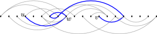
Figure 1: $u$ is weakly $5$-reachable from $v$ by the highlighted path, but $w$ is not weakly reachable from $v$.

The weak $1$-coloring number of a graph is one more than its degeneracy, which is the smallest number $d$ such that every subgraph $H\subseteq G$ has a vertex of degree at most $d$ in $H$. The weak coloring number can be seen as a localized version of tree-depth, as

$$\textnormal{wcol}_{1}(G)\leq\textnormal{wcol}_{2}(G)\leq\dots\leq\textnormal{wcol}_{\infty}(G)=\operatorname{td}(G)\leavevmode\nobreak\ \hbox{\cite[cite]{[\@@bibref{}{sparsity}{}{}]}}.$$

Figure 1 contains an example of weak $r$-reachability. Weak coloring numbers can be used to characterize nowhere dense graph classes:

Proposition 2.4 ([36, 31]).

A graph class $\mathcal{C}$ is nowhere dense if and only if there exists a function $f$ such that for every $r\in{\mathbf{N}}$, every $\varepsilon>0$, every graph $G\in\mathcal{C}$ satisfies $\textnormal{wcol}_{r}(H)\leq f(r,\varepsilon)|H|^{\varepsilon}$ for every $H\subseteq G$.

When weak coloring numbers are used within an algorithm, it is often essential to find an ordering of the vertices of a graph with a small weak coloring number. The situation is similar to efficient algorithms on tree decompositions: First a tree decomposition has to be found. Even though computing $\textnormal{wcol}_{r}(G)$ is NP-hard for $r\geq 3$ in general [20], it is possible to compute in parameterized quasi-linear time orderings which are approximately optimal:

Proposition 2.5 (Grohe, Kreutzer, Siebertz [22, Cor. 5.8]).

Let $\mathcal{C}$ be a nowhere dense graph class. There is a function $f$ such that for all $r\in{\mathbf{N}}$, $\varepsilon>0$ and $G\in\mathcal{C}$ with $|G|\geq f(r,\varepsilon)$, an ordering $\pi$ of $G$ with $|{\rm WReach}_{r}\mathchoice{\mathopen{\hbox{$[$}}}{\mathopen{\hbox{$[$}}}{\mathopen{\hbox{$\scriptstyle[$}}}{\mathopen{\hbox{$\scriptstyle[$}}}G,\pi,v]|\leq|G|^{\varepsilon}$ for all $v\in V(G)$ can be found in time $f(r,\varepsilon)\cdot|G|^{1+\varepsilon}$.

As we are dealing with somewhere dense graph classes in Section 5, we cannot use Proposition 2.5 to construct orderings with small generalized coloring numbers. Revisiting the proof of Proposition 2.5, we notice that even without the assumption of nowhere denseness, one can find in linear time orderings which approximate the weak coloring numbers:

Lemma 2.6.

There is a computable function $f$ and an algorithm that computes for a graph $G$ a vertex ordering $\pi$ such that $\textnormal{wcol}_{r}(G,\pi)\leq\textnormal{wcol}_{f(r)}(G)^{f(r)}$ for every $r\in{\mathbf{N}}$.

The running time of the construction is $\textnormal{wcol}_{f(r)}(G)^{f(r)}|G|$.

Proof 2.7.

We use Theorem 4.6.4 of [34] stating: “For every integer $r>0$ there is a polynomial $q_{r}(x)$ such that for every graph $G$ one can compute in time $q_{r}\bigl{(}\nabla_{2^{r+1}}(G)\bigr{)}$ an orientation ${\smash{\vec{G}}}$ of $G$ and a transitive fraternal augmentation ${\smash{\vec{G}}}_{1}\subseteq\ldots\subseteq{\smash{\vec{G}}}_{r}$ with ${\smash{\vec{G}}}_{1}={\smash{\vec{G}}}$ such that $\Delta^{-}({\smash{\vec{G}}}_{r})\leq q_{r}\bigl{(}\nabla_{2^{r+1}}(G)\bigl{)}$.” The proof is not contained in [34], but follows easily from Corollary 5.3 in [29]. A close look at the proof reveals that the running time is indeed $q_{r}\bigl{(}\nabla_{2^{r+1}}(G)\bigr{)}n$, where $q_{r}$ is a polynomial that is computable given $r$.

Using this result yields a digraph ${\smash{\vec{G}}}_{r}$ such that $\Delta^{-}({\smash{\vec{G}}}_{r})\leq q_{r}\bigl{(}\nabla_{2^{r+1}}(G)\bigl{)}$. Grohe, Kreutzer, and Siebertz show that if ${\smash{\vec{H}}}$ is an $r$-transitive fraternal augmention of a graph $G$ with $\Delta^{-}({\smash{\vec{H}}})\leq d$, then $\textnormal{wcol}_{r}(G)\leq 2(d+1)^{2}$ [22, Lemma 6.7]. Moreover, in the proof of this lemma it is shown that an order can be constructed in linear time that witnesses this bound on the weak coloring number.

Hence, we compute a linear order $\pi$ on the vertices of ${\smash{\vec{G}}}_{r}$ such that

$$\textnormal{wcol}_{r}(G,\pi)\leq 2\bigl{(}q_{r}\bigl{(}\nabla_{2^{r+1}}(G)\bigr{)}+1\bigr{)}^{2}.$$ (3)

The grad $\nabla_{(r-1)/2}(G)$ is bounded by the weak coloring number via $\nabla_{(r-1)/2}(G)+1\leq\textnormal{wcol}_{r}(G)$ [30, Lemma 7.11]. Combining this bound with the bound in (3) yields $\textnormal{wcol}_{r}(G,\pi)\leq 2\bigl{(}q_{r}(\textnormal{wcol}_{2^{r+2}+1}(G)+1)\bigr{)}^{2}\leq\textnormal{wcol}_{2^{r+2}+1}(G)^{f(r)}$ for some $f(r)$.

Altogether we have constructed an ordering $\pi$ in time linear in $||{\smash{\vec{G}}}_{r}||\leq\Delta^{-}({\smash{\vec{G}}}_{r})|G|\leq\textnormal{wcol}_{f(r)}(G)^{f(r)}|G|$ such that $\textnormal{wcol}_{r}(G,\pi)\leq\textnormal{wcol}_{f(r)}(G)^{f(r)}$.

2.4 Splitter game

We will use a game-based characterization of nowhere denseness introduced by Grohe, Kreutzer and Siebertz [22]. Given a graph $G$, a radius $r$ and a number of rounds $\ell$, the $(\ell,r)$-Splitter game on $G$ is an alternating game between two players called Splitter and Connector. The game starts on $G_{0}=G$. In the $i$th round, the Connector chooses a vertex $v_{i}$ from $G_{i}$. Then the Splitter chooses a vertex $s_{i}$ from the radius-$r$ neighborhood of $v_{i}$ in $G_{i}$. The game continues on $G_{i+1}=G_{i}\mathchoice{\mathopen{\hbox{$[$}}}{\mathopen{\hbox{$[$}}}{\mathopen{\hbox{$\scriptstyle[$}}}{\mathopen{\hbox{$\scriptstyle[$}}}v_{i}]-s_{i}$. Splitter wins if after $\ell$ rounds the graph is empty. Grohe, Kreutzer and Siebertz showed that nowhere dense graph classes can be characterized by Splitter games:

Proposition 2.8.

[22] Let ${\mathcal{C}}$ be a nowhere dense class of graphs. Then, for every $r>0$, there is $\ell>0$, such that for every $G\in{\mathcal{C}}$, Splitter has a strategy to win the $(\ell,r)$-splitter game on $G$.

Note that a winning move of Splitter in a current play can be computed in almost linear time [22, Remark 4.7].

2.5 Sparse neighborhood covers

Even though the splitter game ends after a bounded number of rounds $\ell$ for nowhere dense classes, the game tree, i.e. the tree spanned by all possible plays of Splitter and Connector, can still be large, e.g. in the dimensions of $n^{\ell}$. To make the game trees small and useful for algorthmic use, Grohe, Kreutzer and Siebertz introduced sparse neighborhood covers [22]. These covers group “similar” neighborhoods into a small number cluster of bounded radius. These clusters can be used instead of the neighborhoods, reducing the size of the game tree to $O(n^{1+\varepsilon})$.

Definition 2.9.

[22] For a radius $r\in{\mathbf{N}}$, an $r$-neighborhood cover $\mathcal{X}$ of a graph $G$ is a set of connected subgraphs of $G$ called clusters, such that for every vertex $v\in V(G)$ there is some $X\in\mathcal{X}$ with $N_{r}\mathchoice{\mathopen{\hbox{$[$}}}{\mathopen{\hbox{$[$}}}{\mathopen{\hbox{$\scriptstyle[$}}}{\mathopen{\hbox{$\scriptstyle[$}}}v]\subseteq V(X)$. The degree of $v$ in $\mathcal{X}$ is the number of clusters that contain $v$ and the radius of ${\mathcal{X}}$ is the maximal radius of a cover in ${\mathcal{X}}$. A class ${\mathcal{C}}$ admits sparse neighborhood covers if there exists $c\in{\mathbf{N}}$ and for all $r\in{\mathbf{N}}$ and all $\varepsilon>0$ a number $d=d(r,\varepsilon)$ such that every graph $G\in{\mathcal{C}}$ admits an $r$-neighborhood cover of radius at most $c$ and degree at most $d|G|^{\varepsilon}$.

Proposition 2.10.

[22] Every nowhere dense class ${\mathcal{C}}$ of graphs admits a sparse neighborhood cover. For a graph $G\in{\mathcal{C}}$ and $r\in{\mathbf{N}}$ such an $r$-neighborhood cover can be computed in time $f(r,\varepsilon)n^{1+\varepsilon}$ for every $\varepsilon>0$.

Indeed, the existence of such covers is another characterization of nowhere dense classes.

Definition 2.11.

For a graph $G$ with a vertex order $\pi$, $r\in{\mathbf{N}}$ and a vertex $v\in V(G)$, we define $X_{r}\mathchoice{\mathopen{\hbox{$[$}}}{\mathopen{\hbox{$[$}}}{\mathopen{\hbox{$\scriptstyle[$}}}{\mathopen{\hbox{$\scriptstyle[$}}}G,\pi,v]$ as $\{u\in V(G)\mid v\in{\rm WReach}_{r}\mathchoice{\mathopen{\hbox{$[$}}}{\mathopen{\hbox{$[$}}}{\mathopen{\hbox{$\scriptstyle[$}}}{\mathopen{\hbox{$\scriptstyle[$}}}G,\pi,u]\}$. We let $\mathcal{X}_{r}=\{X_{2r}\mathchoice{\mathopen{\hbox{$[$}}}{\mathopen{\hbox{$[$}}}{\mathopen{\hbox{$\scriptstyle[$}}}{\mathopen{\hbox{$\scriptstyle[$}}}G,\pi,v]\mid v\in V(G)\}$.

From the proof of Proposition 2.10 it follows, that the set family $\mathcal{X}_{r}$ is such a sparse neighborhood cover.

2.6 Low treedepth colorings

A crucial algorithmic tool in the study of bounded expansion and nowhere dense graph classes are low treedepth colorings, also known as $r$-centered colorings.

Definition 2.12.

An $r$-treedepth coloring of a graph $G$ is a coloring of vertices of $G$ such that any $r^{\prime}\leq r$ color classes induce a subgraph with treedepth at most $r^{\prime}$.

The following statement by Zhu [36] is modified such that it is constructive and holds also for a given vertex ordering $\pi$. It follows from the original proof.

Proposition 2.13 ([36, Proof of Thm. 2.6]).

If $\pi$ is a vertex ordering of a graph $G$ with $\textnormal{wcol}_{2^{r-2}}(G,\pi)\leq m$, an $r$-treedepth coloring can be computed with at most $m$ colors in time $O(mn)$.

Graph classes of bounded expansion can be characterized by low treedepth colorings, i.e., each graph has an $r$-treedepth coloring with at most $f(r)$ many colors.

2.7 Logic

We are mainly interested in a small fragment of first-order counting logic, namely formulas of the form $\#{y}\,\varphi(y{\bar{x}})>N$ where $\varphi$ is a quantifier-free first-order formula with free variables $y{\bar{x}}$ and $N$ is a natural number.

The length of a formula $\varphi$ is denoted by $|\varphi|$ and equals its number of symbols, where the length of $N$ counts as one. All signatures are finite and the cardinality $|\sigma|$ of a signature $\sigma$ equals the number of its symbols. We often interpret conjunctive clauses $\omega\in{\rm FO}$ as a set of literals and write $l\in\omega$ to indicate that $l$ is a literal of $\omega$.

We denote the universe of a structure $G$ by $V(G)$. We interpret a labeled graph $G=(V,E,P_{1},\dots,P_{m})$ as a logical structure with a universe $V$, binary relation $E$ and unary relations $P_{1},\dots,P_{m}$.

The notation ${\bar{x}}$ stands for a non-empty tuple $x_{1}\dots x_{|{\bar{x}}|}$. We write $\varphi({\bar{x}})$ to indicate that a formula $\varphi$ has free variables ${\bar{x}}$. Let $G$ be a structure, ${\bar{u}}\in V(G)^{|{\bar{x}}|}$ be a tuple of elements from the universe of $G$, and $\beta$ be the assignment with $\beta(x_{i})=u_{i}$ for $i\in\{1,\dots,|{\bar{x}}|\}$. For simplicity, we write $G\models\varphi({\bar{u}})$ and ${\llbracket\varphi({\bar{u}})\rrbracket}^{G}$ instead of $(G,\beta)\models\varphi({\bar{x}})$ and ${\llbracket\varphi({\bar{x}})\rrbracket}^{(G,\beta)}$.

The logic FO is defined in the usual way for functional structures. The functional depth of a formula is the maximum level of nested function applications, e.g., the formula $f(g(x))=y$ has functional depth $2$. We define $FO\mathchoice{\mathopen{\hbox{$[$}}}{\mathopen{\hbox{$[$}}}{\mathopen{\hbox{$\scriptstyle[$}}}{\mathopen{\hbox{$\scriptstyle[$}}}d,\sigma]$ to be all first-order formulas with functional depth $d$ and functional signature $\sigma$.

We will both use functional and relational structures, but we will restrict ourselves to functions of arity one and relations of arity one and two. A structure $G$ with signature $\sigma$ has multiplicity $m$ if for every distinct pair $u,v\in V(G)$, the number of function symbols $f\in\sigma$ with $u=f_{G}(v)$ or $v=f_{G}(u)$ and relation symbols $R\in\sigma$ such that $R^{G}(u,v)$ is at most $m$.

3 Exact Evaluation on Nowhere Dense Classes

In this section we consider the model-checking problem for formulas $\exists x_{1}\dots x_{k}\#{y}\,\varphi(y{\bar{x}})>N$ on nowhere dense graph classes for quantifier-free first-order formulas $\varphi$. We show that this problem can be solved in almost linear fpt time by solving its optimization variant $\max_{{\bar{u}}\in V(G)^{{\bar{x}}}}\#{y}\,{\llbracket\varphi(y{\bar{u}})\rrbracket}$.

3.1 Replace Formulas with Clauses

We start with a simplification of the input formula. The quantifier-free formula $\varphi$ is transformed into a set of weighted positive clauses, i.e. formulas which are conjunctions of positive edge relations with an integer weight assigned to them. The advantage of positive clauses is that each vertex $u$ satisfying $\omega(u{\bar{v}})$ is adjacent to a vertex in ${\bar{u}}$, making the problem very local.

Lemma 3.1.

Consider a quantifier-free FO-formula $\varphi(y{\bar{x}})$ with signature $\sigma$. In time $f(|\varphi|)$ one can construct a set $\Omega$ with the following properties:

1. The set $\Omega$ contains pairs of the form $(\mu,\omega(y{\bar{x}}))$ where $\mu\in{\mathbf{Z}}$ and $\omega(y{\bar{x}})$ is a conjunctive clause containing only positive literals,

2. $|\Omega|\leq 4^{|\varphi|}$,

3. $|\omega|\leq|\varphi|$ for each $(\mu,\omega)\in\Omega$,

4. $|\mu|\leq 4^{|\varphi|}$ for every $(\mu,\omega)\in\Omega$,

5. for every graph $G$ and every ${\bar{u}}\in V(G)^{|{\bar{x}}|}$,
   $\displaystyle{\llbracket\#{y}\,\varphi(y{\bar{u}})\rrbracket}^{G}=\sum_{\mathclap{(\mu,\omega)\in\Omega}}\mu{\llbracket\#{y}\,\omega(y{\bar{u}})\rrbracket}^{G}.$

Proof 3.2.

Let $L$ be the set of literals in $\varphi$. We construct a formula $\varphi^{\prime}$, equivalent to $\varphi$, in disjunctive normal form (disjunction of conjunctions). We can assume $\varphi^{\prime}$ to be complete in the sense that every atom in $L$ occurs in every clause of $\varphi^{\prime}$ (either positively or negatively). Thus, every clause of $\varphi^{\prime}$ contains $|L|\leq|\varphi|$ literals. For every conjunctive clause $\omega$ of $\varphi^{\prime}$ we add the tuple $(1,\omega)$ into a set $\Omega$. Since by completeness the clauses of $\varphi^{\prime}$ are mutually exclusive,

$${\llbracket\#{y}\,\varphi(y{\bar{u}})\rrbracket}^{G}=\sum_{(\mu,\omega)\in\Omega}\mu{\llbracket\#{y}\,\omega(y{\bar{u}})\rrbracket}^{G}.$$ (4)

Fix a tuple $(\mu,\omega)\in\Omega$. Unless $\omega$ contains only positive literals, we can write it as $\omega^{\prime}\land\neg l$, where $l$ is a positive literal. By first ignoring $l$ and then subtracting what we counted too much we get

$$\mu{\llbracket\#y\,\omega(y{\bar{x}})\rrbracket}^{{\smash{\vec{G}}}}=\mu{\llbracket\#y\,\omega^{\prime}(y{\bar{x}})\land l\rrbracket}^{G}-\mu{\llbracket\#y\,\omega^{\prime}(y{\bar{x}})\rrbracket}^{G}.$$ (5)

We remove $(\mu,\omega)$ from $\Omega$ and add two new entries with conjunctive clauses as in (5) such that $\Omega$ still satisfies (4). Both newly introduced formulas contain one negative literal less. It can happen that we want to add some $(\mu,\omega^{\prime})$ to $\Omega$ when $\Omega$ already contains $(\mu^{\prime},\omega^{\prime})$. In that case we replace the latter by $(\mu+\mu^{\prime},\omega^{\prime})$.

We perform this procedure on $\Omega$ until no longer possible. The length of each clause in $\Omega$ is still at most $|\varphi|$. The size of $\Omega$ is at most $4^{|\varphi|}$ as the complete DNF formula $\varphi^{\prime}$ has at most $2^{|\varphi|}$ clauses of length at most $|\varphi|$, and applying the previously described inclusion-exclusion steps exhaustively to one clause results in at most $2^{|\varphi|}$ new clauses.

As the bound for $|\Omega|$ follows from counting the resulting clauses (without deduplicating possible duplicates), the same bound of $4^{\varphi}$ also follows for the weights.

3.2 Radius-$r$ Decomposition Tree

In the following, we will introduce a new kind of decomposition, which heavily relies on the ideas from [22]. We call it the radius-$r$ decomposition tree. For illustration, consider a tree-depth decomposition of a graph $G$. It has the property that after the removal of the root $v$ in the decomposition, for each connected component $C$ of $G-v$ there exists a child of $v$ in the decomposition that contains $C$. In the radius-$r$ decomposition tree, not every connected component is represented by a child but every radius-$r$ neighborhood of $G-v$ instead. Another difference is that these neighborhoods are not necessarily disjoint. We will use this radius-$r$ decomposition tree as the structure on which a dynamic program will solve $\max_{{\bar{u}}}{\llbracket\#{y}\,\varphi(y{\bar{u}})\rrbracket}^{G}$.

Definition 3.3.

Let $G$ be a graph. Let $r,\ell\in{\mathbf{N}}$ be such that splitter has a winning strategy for the $\ell$-round radius-$2r$ splitter game on $G$. Let $\pi$ be an ordering of $G$.

A radius-$r$ decomposition tree $T_{r}(G,\pi,\ell)$ is a pair $(T,\beta)$ where $T$ is a tree of depth $\ell$ and $\beta\colon V(T)\to V(G)$. We construct it recursively. If $G$ is empty, $T_{r}(G,\pi,\ell)$ is the empty tree.

Let $s\in V(G)$ be the first move of the winning strategy of splitter for the $(\ell,2r)$-splitter game on $G$. The root is a node $t$ with $\beta(t)=s$. For every $v\in V(G)$ we append the decomposition tree $T_{r}(G\mathchoice{\mathopen{\hbox{$[$}}}{\mathopen{\hbox{$[$}}}{\mathopen{\hbox{$\scriptstyle[$}}}{\mathopen{\hbox{$\scriptstyle[$}}}X_{v}],\pi,\ell-1)$ where $X_{v}=X_{2r}\mathchoice{\mathopen{\hbox{$[$}}}{\mathopen{\hbox{$[$}}}{\mathopen{\hbox{$\scriptstyle[$}}}{\mathopen{\hbox{$\scriptstyle[$}}}G-s,\pi,v]$.

Note that the case $\ell=0$ while the graph is not empty, cannot happen due to the Splitter having a winning strategy.

Corollary 3.4.

Let $G$ be a graph, $\pi$ a vertex ordering of $G$, $r,\ell\in{\mathbf{N}}$ and $T=T_{r}(G,\pi,\ell)$ a radius-$r$ decomposition tree. Let $t\in V(T)$ be a node and $T_{t}$ be the subtree of $T$ starting at $t$. Then for every $u\in W:=\beta(V(T_{t}))\setminus\{\beta(t)\}$ there exists a child $t^{\prime}$ of $t$ such that $N_{r}^{G\mathchoice{\mathopen{\hbox{$[$}}}{\mathopen{\hbox{$[$}}}{\mathopen{\hbox{$\scriptstyle[$}}}{\mathopen{\hbox{$\scriptstyle[$}}}W]}\mathchoice{\mathopen{\hbox{$[$}}}{\mathopen{\hbox{$[$}}}{\mathopen{\hbox{$\scriptstyle[$}}}{\mathopen{\hbox{$\scriptstyle[$}}}u]\subseteq\beta(T_{t^{\prime}})$.

As $\mathcal{X}_{r}=\{X_{2r}\mathchoice{\mathopen{\hbox{$[$}}}{\mathopen{\hbox{$[$}}}{\mathopen{\hbox{$\scriptstyle[$}}}{\mathopen{\hbox{$\scriptstyle[$}}}G,\pi,v]\mid v\in V(G)\}$ is by Proposition 2.10 a radius-$r$ cover, the fact follows immediately.

Lemma 3.5.

Let $G$ be a graph, $\pi$ a vertex ordering of $G$ and $r,\ell\in{\mathbf{N}}$. Then, the radius-$r$ decomposition tree $T=T_{r}(G,\pi,\ell)$ (Definition 3.3) has size $|T|\leq\textnormal{wcol}_{2r}(G,\pi)^{\ell}n$ and depth $\ell$. The construction time is linear in $|T|$.

Proof 3.6.

By construction, the depth of the tree is determined by the depth of the splitter game, which is $\ell$.

Consider the root path $P_{t}$ of some node $t\in V(T)$. Then $\beta(P_{t})\subseteq{\rm WReach}_{2r}\mathchoice{\mathopen{\hbox{$[$}}}{\mathopen{\hbox{$[$}}}{\mathopen{\hbox{$\scriptstyle[$}}}{\mathopen{\hbox{$\scriptstyle[$}}}G,\pi,\beta(t)]$. As the length of $P_{t}$ is at most $\ell$, $\beta(t)$ appears at most ${\rm WReach}_{2r}\mathchoice{\mathopen{\hbox{$[$}}}{\mathopen{\hbox{$[$}}}{\mathopen{\hbox{$\scriptstyle[$}}}{\mathopen{\hbox{$\scriptstyle[$}}}G,\pi,\beta(t)]^{\ell}\leq\textnormal{wcol}_{2r}(G,\pi)^{\ell}$ times (as a $\beta$-label of nodes) in $T$. Thus, $|T|\leq\textnormal{wcol}_{2r}(G,\pi)^{\ell}n$.

Corollary 3.7.

Let $\mathcal{C}$ be a nowhere dense graph class. For every $r\in{\mathbf{N}}$ the $r$-decomposition tree has constant depth, almost linear size and can be computed in almost linear time.

3.3 Cover Systems

Given a subgraph $H$ in $G$ with a vertex ordering $\pi$ of $G$. A cover system of $H$ in $G$ is a family $\mathcal{Z}$ of clusters $Z_{i}=X_{r}\mathchoice{\mathopen{\hbox{$[$}}}{\mathopen{\hbox{$[$}}}{\mathopen{\hbox{$\scriptstyle[$}}}{\mathopen{\hbox{$\scriptstyle[$}}}G,\pi,v]\in Z$ for some $r\in{\mathbf{N}}$ such that every connected component $C$ of $H$ is contained in some $Z_{i}$. A cover system is non-overlapping if all distinct clusters have an empty intersection.

Lemma 3.8.

For every graph $G$ with a vertex ordering $\pi$, every $D\subseteq V(G)$ of size $k$, there exists a cover system of $G\mathchoice{\mathopen{\hbox{$[$}}}{\mathopen{\hbox{$[$}}}{\mathopen{\hbox{$\scriptstyle[$}}}{\mathopen{\hbox{$\scriptstyle[$}}}N\mathchoice{\mathopen{\hbox{$[$}}}{\mathopen{\hbox{$[$}}}{\mathopen{\hbox{$\scriptstyle[$}}}{\mathopen{\hbox{$\scriptstyle[$}}}D]]$ in $G$ of size at most $k$ where each cluster has the same radius $r\leq 2^{k}$.

Proof 3.9.

We start with the clusters $X_{2}\mathchoice{\mathopen{\hbox{$[$}}}{\mathopen{\hbox{$[$}}}{\mathopen{\hbox{$\scriptstyle[$}}}{\mathopen{\hbox{$\scriptstyle[$}}}G,\pi,\min_{\pi}N\mathchoice{\mathopen{\hbox{$[$}}}{\mathopen{\hbox{$[$}}}{\mathopen{\hbox{$\scriptstyle[$}}}{\mathopen{\hbox{$\scriptstyle[$}}}d]]$ for every $d\in D$. Call this collection $\mathcal{Z}$. Note that $\mathcal{Z}$ is already a valid cover system of $G\mathchoice{\mathopen{\hbox{$[$}}}{\mathopen{\hbox{$[$}}}{\mathopen{\hbox{$\scriptstyle[$}}}{\mathopen{\hbox{$\scriptstyle[$}}}N\mathchoice{\mathopen{\hbox{$[$}}}{\mathopen{\hbox{$[$}}}{\mathopen{\hbox{$\scriptstyle[$}}}{\mathopen{\hbox{$\scriptstyle[$}}}D]]$ in $G$. If two distinct clusters $X_{r}\mathchoice{\mathopen{\hbox{$[$}}}{\mathopen{\hbox{$[$}}}{\mathopen{\hbox{$\scriptstyle[$}}}{\mathopen{\hbox{$\scriptstyle[$}}}G,\pi,z]$ and $X_{r}\mathchoice{\mathopen{\hbox{$[$}}}{\mathopen{\hbox{$[$}}}{\mathopen{\hbox{$\scriptstyle[$}}}{\mathopen{\hbox{$\scriptstyle[$}}}G,\pi,z^{\prime}]$ from $\mathcal{Z}$ intersect, we replace both with a new cluster $X_{2r}\mathchoice{\mathopen{\hbox{$[$}}}{\mathopen{\hbox{$[$}}}{\mathopen{\hbox{$\scriptstyle[$}}}{\mathopen{\hbox{$\scriptstyle[$}}}G,\pi,\min_{\pi}\{z,z^{\prime}\}]$ in $\mathcal{Z}$. Every vertex or edge covered by the two old clusters stays covered in the new one. Also, if two clusters $X_{r}\mathchoice{\mathopen{\hbox{$[$}}}{\mathopen{\hbox{$[$}}}{\mathopen{\hbox{$\scriptstyle[$}}}{\mathopen{\hbox{$\scriptstyle[$}}}G,\pi,z]$ and $X_{r^{\prime}}\mathchoice{\mathopen{\hbox{$[$}}}{\mathopen{\hbox{$[$}}}{\mathopen{\hbox{$\scriptstyle[$}}}{\mathopen{\hbox{$\scriptstyle[$}}}G,\pi,z^{\prime}]$ are of a different radius, say, $r^{\prime}<r$, we replace $X_{r^{\prime}}\mathchoice{\mathopen{\hbox{$[$}}}{\mathopen{\hbox{$[$}}}{\mathopen{\hbox{$\scriptstyle[$}}}{\mathopen{\hbox{$\scriptstyle[$}}}G,\pi,z^{\prime}]$ with $X_{r}\mathchoice{\mathopen{\hbox{$[$}}}{\mathopen{\hbox{$[$}}}{\mathopen{\hbox{$\scriptstyle[$}}}{\mathopen{\hbox{$\scriptstyle[$}}}G,\pi,z^{\prime}]$ to match the radii of all the clusters.

We repeat this until no intersecting clusters remain. As the number of clusters decreases with every step, the radius is at most $2^{k}$ at the end.

For Theorem 1.1, one needs to find clusters from $\mathcal{X}_{r}$ which are disjoint and maximize the sum of weights of clusters. This is captured by the following definition. We can solve this problem in almost linear time on nowhere dense graph classes, by noticing that the intersection graphs of the sparse neighborhood covers $\mathcal{X}_{r}$ are almost nowhere dense. Then, one can use treedepth colorings and LinEMSOL.

Definition 3.10 (Disjoint Cluster Maximization).

Given a graph, a set system $\mathcal{X}_{r}$ as defined in Definition 2.11, labelled by a function $\Lambda:\mathcal{X}_{r}\to 2^{\Lambda}$ of size $k$. Each combination of a cluster $X\in\mathcal{X}_{r}$ and label $\lambda\in\Lambda(X)$ is weighted by a function $w$.

Problem: Find pairwise disjoint clusters $X_{1},\dots,X_{k}\in\mathcal{X}_{r}$ such that for each label $\lambda_{i}\in\Lambda$ the cluster $X_{i}$ is labeled $\lambda_{i}$ and $X_{1},\dots,X_{k}$ maximize $\sum_{i=1}^{k}w(X_{i},\lambda_{i})$ for such cluster sets.

Parameter: $r,k$

Lemma 3.11.

Let $\mathcal{C}$ be a nowhere dense class of graphs and $r\in{\mathbf{N}}$. Then there exists an almost nowhere dense graph class $\mathcal{I}$ such that for every graph $G\in\mathcal{C}$, the intersection graph $I$ of $\mathcal{X}_{r}$ (defined in Definition 2.11) is contained in $\mathcal{I}$.

Proof 3.12.

Assume $\prec$ witnesses a good order in $G$. We build a new order $\prec_{I}$ for $I$. $X_{r}\mathchoice{\mathopen{\hbox{$[$}}}{\mathopen{\hbox{$[$}}}{\mathopen{\hbox{$\scriptstyle[$}}}{\mathopen{\hbox{$\scriptstyle[$}}}v]$ is a shorthand for $X_{r}\mathchoice{\mathopen{\hbox{$[$}}}{\mathopen{\hbox{$[$}}}{\mathopen{\hbox{$\scriptstyle[$}}}{\mathopen{\hbox{$\scriptstyle[$}}}G,\prec,v]$. We say $X_{r}\mathchoice{\mathopen{\hbox{$[$}}}{\mathopen{\hbox{$[$}}}{\mathopen{\hbox{$\scriptstyle[$}}}{\mathopen{\hbox{$\scriptstyle[$}}}v]\prec_{I}X_{r}\mathchoice{\mathopen{\hbox{$[$}}}{\mathopen{\hbox{$[$}}}{\mathopen{\hbox{$\scriptstyle[$}}}{\mathopen{\hbox{$\scriptstyle[$}}}u]$ if $v\prec u$. Then

$${\rm WReach}_{s}\mathchoice{\mathopen{\hbox{$[$}}}{\mathopen{\hbox{$[$}}}{\mathopen{\hbox{$\scriptstyle[$}}}{\mathopen{\hbox{$\scriptstyle[$}}}I,\prec_{I},X_{r}\mathchoice{\mathopen{\hbox{$[$}}}{\mathopen{\hbox{$[$}}}{\mathopen{\hbox{$\scriptstyle[$}}}{\mathopen{\hbox{$\scriptstyle[$}}}u]] =\{Y\in\mathcal{X}\mid\text{path $P=Y_{0}\dots Y_{s}$ of length at most $s$ in $I$},$$

$$\qquad Y_{0}=X_{r}\mathchoice{\mathopen{\hbox{$[$}}}{\mathopen{\hbox{$[$}}}{\mathopen{\hbox{$\scriptstyle[$}}}{\mathopen{\hbox{$\scriptstyle[$}}}u],Y_{s}=Y=\min_{\prec_{I}}P\}$$

$$\subseteq\{X_{r}\mathchoice{\mathopen{\hbox{$[$}}}{\mathopen{\hbox{$[$}}}{\mathopen{\hbox{$\scriptstyle[$}}}{\mathopen{\hbox{$\scriptstyle[$}}}v]\in\mathcal{X}\mid v\in{\rm WReach}_{2rs}\mathchoice{\mathopen{\hbox{$[$}}}{\mathopen{\hbox{$[$}}}{\mathopen{\hbox{$\scriptstyle[$}}}{\mathopen{\hbox{$\scriptstyle[$}}}G,\prec,u]\}$$

Note that $v=\min_{\prec}X_{r}\mathchoice{\mathopen{\hbox{$[$}}}{\mathopen{\hbox{$[$}}}{\mathopen{\hbox{$\scriptstyle[$}}}{\mathopen{\hbox{$\scriptstyle[$}}}v]$. Hence, the last equation follows. As ${\rm WReach}_{2rs}\mathchoice{\mathopen{\hbox{$[$}}}{\mathopen{\hbox{$[$}}}{\mathopen{\hbox{$\scriptstyle[$}}}{\mathopen{\hbox{$\scriptstyle[$}}}G,\prec,u]\leq n^{\varepsilon}$, so is ${\rm WReach}_{s}\mathchoice{\mathopen{\hbox{$[$}}}{\mathopen{\hbox{$[$}}}{\mathopen{\hbox{$\scriptstyle[$}}}{\mathopen{\hbox{$\scriptstyle[$}}}I,\prec_{I},X_{r}\mathchoice{\mathopen{\hbox{$[$}}}{\mathopen{\hbox{$[$}}}{\mathopen{\hbox{$\scriptstyle[$}}}{\mathopen{\hbox{$\scriptstyle[$}}}u]]$. Thus, $\mathcal{I}$ is almost nowhere dense.

Remark 3.13.

Note that this result cannot be improved to a nowhere dense class of intersection graphs for $\mathcal{X}_{r}$. However, maybe there exists another sparse neighborhood cover whose intersection graph is nowhere dense.

Example: Consider the class of graphs with an independent set of size $n$ with a star of size of $\log n$. For the weak color ordering, order the apex to the right (this is not optimal but the weak coloring number of this ordering is $\log n$). The resulting intersection graph contains then a clique of size $n$. Hence, the which is somewhere dense.

Lemma 3.14.

We can solve the Disjoint Cluster Maximization problem in almost linear FPT time on nowhere dense class of graphs.

Proof 3.15.

As $G$ is from a nowhere dense graph class, we can apply Lemma 3.11, yielding a graph $H$ from an almost nowhere dense graph class. The labels and weights from $G$ are also added to $H$.

Two clusters $X,Y\in\mathcal{X}_{r}$ are disjoint in $G$ if and only if $X$ and $Y$ are not adjacent in $H$. Hence, the original problem on $G$ is equivalent to finding an independent set $S$ of size in $H$, where $\sum_{i}w(S_{i},\lambda_{i})$ is maximized.

Since $H$ is from an almost nowhere dense graph class, by Proposition 2.13 there exists a $k$-treedepth coloring of $H$ using $n^{\varepsilon}$ many colors. As the optimal independent set $S$ with the constraints from above has size $k$, it has to be contained in the subgraph of $H$ induced by some selection of at most $k$ colors. Thus, for each selection of $k$ colors, we consider the graph $H^{\prime}$ induced by those which has treedepth at most $k$. As this independent set variation can be expressed as MSO-formula and the objective function is linear, we can use LinEMSOL on $H^{\prime}$ to solve this problem optimally. The solution for $H$ is then the maximum over the solutions of all $H^{\prime}$s.

Applying Lemma 3.11 takes almost linear time. There are ${n^{\varepsilon}\choose k}\leq n^{\varepsilon^{\prime}}$ many color combinations and each iteration of LinEMSOL takes linear FPT time.

Let $\Omega$ be the set of weighted positive conjunctive clauses $(\mu,\omega(y{\bar{x}}))$, ${\bar{z}}\subseteq{\bar{x}}$ and ${\bar{u}}\in V(G)^{|{\bar{x}}|}$. With $\Omega|_{{\bar{z}}}$ we denote a subset of $\Omega$ with weighted clauses $(\mu,\omega(y{\bar{x}}))$ where every variable occurring in $\omega$ is from ${\bar{z}}$. We define $\Omega|_{{\bar{z}}}\mathchoice{\mathopen{\hbox{$[$}}}{\mathopen{\hbox{$[$}}}{\mathopen{\hbox{$\scriptstyle[$}}}{\mathopen{\hbox{$\scriptstyle[$}}}Z,{\bar{u}}]$ as $\sum_{v\in Z}\sum_{(\mu,\omega)\in\Omega|_{{\bar{z}}}}\mu{\llbracket\omega(v{\bar{u}})\rrbracket}^{G}$. Note that $\Omega|_{{\bar{z}}}\mathchoice{\mathopen{\hbox{$[$}}}{\mathopen{\hbox{$[$}}}{\mathopen{\hbox{$\scriptstyle[$}}}{\mathopen{\hbox{$\scriptstyle[$}}}Z,{\bar{u}}]$ depends only on the assignment of ${\bar{z}}$ and does not need the full assignment ${\bar{u}}$ of ${\bar{x}}$.

To illustrate the following lemma, consider a positive conjunctive clause $\omega(y{\bar{x}}{\bar{z}})$, sets $P,W\subseteq V(G)$ and ${\bar{u}}\in P^{\bar{x}},{\bar{w}}\in W^{\bar{z}}$. To count the fulfilling vertices $v\in W$ of $\omega$, i.e. $\Omega\mathchoice{\mathopen{\hbox{$[$}}}{\mathopen{\hbox{$[$}}}{\mathopen{\hbox{$\scriptstyle[$}}}{\mathopen{\hbox{$\scriptstyle[$}}}W,{\bar{u}}]$, we want to reduce this task to counting on cover systems of $N\mathchoice{\mathopen{\hbox{$[$}}}{\mathopen{\hbox{$[$}}}{\mathopen{\hbox{$\scriptstyle[$}}}{\mathopen{\hbox{$\scriptstyle[$}}}{\bar{w}}]$. However, as not all fulfilling vertices in $W$ are adjacent to ${\bar{w}}$, we need to be more careful.

Lemma 3.16.

Let $G$ be a graph, $\Omega$ a set of weighted positive conjunctive clauses $(\mu,\omega(y{\bar{x}}{\bar{z}}))$, $P,W\subseteq V(G)$ disjoint, ${\bar{u}}\in P^{{\bar{x}}},{\bar{w}}\in W^{{\bar{z}}}$ such that $N\mathchoice{\mathopen{\hbox{$[$}}}{\mathopen{\hbox{$[$}}}{\mathopen{\hbox{$\scriptstyle[$}}}{\mathopen{\hbox{$\scriptstyle[$}}}{\bar{w}}]\subseteq P\cup W$. For every cover system $\mathcal{Z}$ of $G\mathchoice{\mathopen{\hbox{$[$}}}{\mathopen{\hbox{$[$}}}{\mathopen{\hbox{$\scriptstyle[$}}}{\mathopen{\hbox{$\scriptstyle[$}}}N\mathchoice{\mathopen{\hbox{$[$}}}{\mathopen{\hbox{$[$}}}{\mathopen{\hbox{$\scriptstyle[$}}}{\mathopen{\hbox{$\scriptstyle[$}}}{\bar{w}}]]$ in $G\mathchoice{\mathopen{\hbox{$[$}}}{\mathopen{\hbox{$[$}}}{\mathopen{\hbox{$\scriptstyle[$}}}{\mathopen{\hbox{$\scriptstyle[$}}}W]$ it holds that

$$\Omega\mathchoice{\mathopen{\hbox{$[$}}}{\mathopen{\hbox{$[$}}}{\mathopen{\hbox{$\scriptstyle[$}}}{\mathopen{\hbox{$\scriptstyle[$}}}W,{\bar{u}}{\bar{w}}]=\Omega|_{y{\bar{x}}}\mathchoice{\mathopen{\hbox{$[$}}}{\mathopen{\hbox{$[$}}}{\mathopen{\hbox{$\scriptstyle[$}}}{\mathopen{\hbox{$\scriptstyle[$}}}W,{\bar{u}}{\bar{w}}]+\sum_{Z\in\mathcal{Z}}(\Omega|_{y{\bar{x}}{\bar{z}}_{Z}}\mathchoice{\mathopen{\hbox{$[$}}}{\mathopen{\hbox{$[$}}}{\mathopen{\hbox{$\scriptstyle[$}}}{\mathopen{\hbox{$\scriptstyle[$}}}Z,{\bar{u}}{\bar{w}}]-\Omega|_{y{\bar{x}}}\mathchoice{\mathopen{\hbox{$[$}}}{\mathopen{\hbox{$[$}}}{\mathopen{\hbox{$\scriptstyle[$}}}{\mathopen{\hbox{$\scriptstyle[$}}}Z,{\bar{u}}])$$

where ${\bar{z}}_{Z}$ are the variables $z_{i}$ from ${\bar{z}}$ which are assigned to a vertex in $Z$.

Proof 3.17.

For $u\in W$, $G\models\omega(u{\bar{u}}{\bar{w}})$ only if $u$ is adjacent to some vertex from ${\bar{u}}{\bar{w}}$, as $\omega$ is a positive conjunctive clause. Hence, $\Omega\mathchoice{\mathopen{\hbox{$[$}}}{\mathopen{\hbox{$[$}}}{\mathopen{\hbox{$\scriptstyle[$}}}{\mathopen{\hbox{$\scriptstyle[$}}}W\setminus N\mathchoice{\mathopen{\hbox{$[$}}}{\mathopen{\hbox{$[$}}}{\mathopen{\hbox{$\scriptstyle[$}}}{\mathopen{\hbox{$\scriptstyle[$}}}{\bar{w}}],{\bar{u}}{\bar{w}}]=\Omega|_{y{\bar{x}}}\mathchoice{\mathopen{\hbox{$[$}}}{\mathopen{\hbox{$[$}}}{\mathopen{\hbox{$\scriptstyle[$}}}{\mathopen{\hbox{$\scriptstyle[$}}}W\setminus N\mathchoice{\mathopen{\hbox{$[$}}}{\mathopen{\hbox{$[$}}}{\mathopen{\hbox{$\scriptstyle[$}}}{\mathopen{\hbox{$\scriptstyle[$}}}{\bar{w}}],{\bar{u}}{\bar{w}}]$. This also holds for $N\setminus\bigcup\mathcal{Z}$ instead. By the same observation $\Omega\mathchoice{\mathopen{\hbox{$[$}}}{\mathopen{\hbox{$[$}}}{\mathopen{\hbox{$\scriptstyle[$}}}{\mathopen{\hbox{$\scriptstyle[$}}}Z,{\bar{u}}{\bar{w}}]=\Omega|_{y{\bar{x}}{\bar{z}}_{Z}}$ for $Z\in\mathcal{Z}$. We get the equality as a result of the observation above and subtracting $\Omega|_{y{\bar{x}}}\mathchoice{\mathopen{\hbox{$[$}}}{\mathopen{\hbox{$[$}}}{\mathopen{\hbox{$\scriptstyle[$}}}{\mathopen{\hbox{$\scriptstyle[$}}}Z,{\bar{u}}{\bar{w}}]$ to prevent counting vertices in $Z$ twice.

Let us consider how a solution ${\bar{u}}$ for $\#{y}\,\varphi(y{\bar{x}})$ interacts with a radius-$r$ decomposition of the input graph $G$ where $r$ is chosen appropriately big, e.g. $2^{k}$ resulting from Lemma 3.8. First, we transform $\varphi$ into a set of positive clauses $\Omega$using Lemma 3.1, making the application of Lemma 3.16 possible.

Consider some node $t$ in $T_{r}$. When applying Lemma 3.16 with $P$ as the vertices of the root path of $t$ and $W$ as $T_{t}$, we see that the resulting cover system $\mathcal{Z}$ corresponds to a selection of children of $t$ in $T_{r}$, as both use the sets $X_{r}$ from Definition 2.11. Now imagine that we know $\Omega_{y{\bar{x}}{\bar{z}}_{Z}}\mathchoice{\mathopen{\hbox{$[$}}}{\mathopen{\hbox{$[$}}}{\mathopen{\hbox{$\scriptstyle[$}}}{\mathopen{\hbox{$\scriptstyle[$}}}Z,{\bar{u}}]$ for every $Z\in\mathcal{Z}$. Note that this number only depends on the assignment of ${\bar{x}}{\bar{z}}_{z}$ and not the vertices assigned outside $P$ and $Z$. With Lemma 3.16 we can combine these numbers into $\Omega\mathchoice{\mathopen{\hbox{$[$}}}{\mathopen{\hbox{$[$}}}{\mathopen{\hbox{$\scriptstyle[$}}}{\mathopen{\hbox{$\scriptstyle[$}}}W,{\bar{u}}]$ without needing to know the actual assignments of ${\bar{z}}_{Z}$ in the cover system anymore! Note that $\Omega_{y{\bar{x}}}\mathchoice{\mathopen{\hbox{$[$}}}{\mathopen{\hbox{$[$}}}{\mathopen{\hbox{$\scriptstyle[$}}}{\mathopen{\hbox{$\scriptstyle[$}}}Z]$ is easily computable while only knowing ${\bar{u}}$ and not ${\bar{w}}$.

Thus, we can compute ${\llbracket\#{y}\,\varphi(y{\bar{u}})\rrbracket}$ bottom-up using the radius-$r$ decomposition while only considering the vertices assigned in ${\bar{u}}$ which are contained in the root path of the considered vertex.

3.4 Dynamic Program

To determine $\max_{{\bar{u}}}\#{y}\,\varphi(y{\bar{u}})$ for a quantifier-free formula $\varphi(y{\bar{x}})$ we recursively compute the following information in the decomposition tree of $G$ (bottom-up, if you will). Consider some node $t$ of $T$ and a partial assignment $\alpha$ of ${\bar{x}}$ to the root path $\beta(P_{t})$. The interesting information is: How many vertices underneath $t$, i.e. in $V(G_{t})$, fulfill $\varphi$ under the “best” choice on completing the assignment $\alpha$ to vertices in $V(G_{t})$. Then the answer to the problem can be read off the information for the root node.

Assume we already know this kind of information for every child $t^{\prime}$ of $t$. To compute this information for $t$, we branch how the variables $x_{i}$ that are not assigned under $\alpha$ are distributed among the children of $t$. Then the table entries of these children are combined in a suitable way. We do this for every distribution among children and take the maximum of the resulting values. If a vertex corresponding to $t$ fulfills with the assignment the formula $\varphi$, it gets counted towards the number of “fulfilling” vertices.

However, we have to take more into consideration. First, branching on the distribution of the unassigned variables $x_{i}$s under $\alpha$ among the children of $t$ is not fast enough, as there are around $n^{k}$ possibilities for that. Instead, we branch on how the unassigned variables are partitioned. For every such partition, we formalize the optimal choice of children $t_{i}$ such that they contain exactly the unassigned variables from the $i$-th part, as an optimization problem.

Secondly, the graphs $G_{t^{\prime}}$ spanned by each child $t^{\prime}$ of $t$ are in general not disjoint. Combining the counts of two overlapping graphs yields to double counting. We circumvent this in the above optimization problem.

Thirdly, we need to keep track of how the vertices in the root path $P_{t}$ are adjacent to the variables $x_{i}$ that are assigned underneath $t$. We cannot branch on the complete assignment as the number of those is too high.

Before we turn to the dynamic program on the decomposition tree, we consider something simpler:

Let $G$ be a graph and $\varphi(y{\bar{x}})$ be quantifier-free FO formula. Consider the pair $(P,W)$ which is a set of vertices $P=\{v_{1},\dots,v_{k}\}\subseteq V(G)$ and a set $W\subseteq V(G)$ that is disjoint with $P$. We are interested in how many vertices $v$ in $G\mathchoice{\mathopen{\hbox{$[$}}}{\mathopen{\hbox{$[$}}}{\mathopen{\hbox{$\scriptstyle[$}}}{\mathopen{\hbox{$\scriptstyle[$}}}P\cup W]$ satisfy $\varphi(v{\bar{u}})$ for an optimal choice of ${\bar{u}}\in(P\cup W)^{|{\bar{u}}|}$. For this, we keep track of $M_{\alpha}^{(P,W)}\mathchoice{\mathopen{\hbox{$[$}}}{\mathopen{\hbox{$[$}}}{\mathopen{\hbox{$\scriptstyle[$}}}{\mathopen{\hbox{$\scriptstyle[$}}}S]$, which is the number of fulfilling vertices $v\in W$ wrt. $\varphi$, $\hat{\alpha}$ and $S$, maximizing over $S$-completions $\hat{\alpha}$ on $W$.

We can “forget” a vertex $v$, i.e., derive the information of $(P,W\cup\{v\})$ from the information $(P\cup\{v\},W)$ as follows: Assume the maximum number of fulfilling vertices in $W$ is $x$ for a given partial assignment $\alpha$ on $P\cup\{v\}$ and adjacency profile $S$ on $P\cup\{v\}$. Then the number of fulfilling vertices in $W\cup\{v\}$ is $x+1$ if $v$ satisfies $\varphi$ with the assignment $\alpha$ and adjacency profile $S$, or $x$ otherwise. However, neither $\alpha$ nor $S$ are valid assignments or adjacency profiles for $P$. Hence, we need to adjust these so that we can formulate this information for $(P,W\cup\{v\})$. For this, we need to remove $v$ from $\alpha$ and add the neighborhood of $v$ in $P$ to $S$ as $S_{i}$, for every $i$ with $\alpha(x_{i})=v$. Then, $M_{\alpha}^{(P\cup\{v\},W)}\mathchoice{\mathopen{\hbox{$[$}}}{\mathopen{\hbox{$[$}}}{\mathopen{\hbox{$\scriptstyle[$}}}{\mathopen{\hbox{$\scriptstyle[$}}}S]=M_{\alpha|_{P}}^{(P,W\cup\{v\})}\mathchoice{\mathopen{\hbox{$[$}}}{\mathopen{\hbox{$[$}}}{\mathopen{\hbox{$\scriptstyle[$}}}{\mathopen{\hbox{$\scriptstyle[$}}}S^{\prime}](+1)$ where $\alpha|_{P}$ is the assignment $\alpha$ without $v$ and $S^{\prime}$ is the adjacency profile as described above.

One can also combine the information of two structures $(P,W_{1})$ and $(P,W_{2})$ to get the information of $(P,W_{1}\uplus W_{2})$ if $W_{1}$ and $W_{2}$ are disjoint. This is also known as “merge.” Consider some assignment $\alpha$ on $P$ and some adjacency profile $S$ on $P$. Then the number of fulfilling vertices in $U\uplus W$ wrt $\varphi$, $\alpha$ and $S$ is the $\max\{M_{\alpha}^{P,W_{1}}\mathchoice{\mathopen{\hbox{$[$}}}{\mathopen{\hbox{$[$}}}{\mathopen{\hbox{$\scriptstyle[$}}}{\mathopen{\hbox{$\scriptstyle[$}}}S_{1}]+M_{\alpha}^{P,W_{2}}\mathchoice{\mathopen{\hbox{$[$}}}{\mathopen{\hbox{$[$}}}{\mathopen{\hbox{$\scriptstyle[$}}}{\mathopen{\hbox{$\scriptstyle[$}}}S_{2}]\mid S_{1}\uplus S_{2}=S\}$.

Indeed however, the algorithm does not take a quantifier-free formula $\varphi$ but a set of weighted positive conjunctive clauses. Instead of just counting the fulfilled vertices, it computes the added up weight of them wrt. to the weights of the clauses.

3.4.1 Some definitions

Let $I\subseteq{\mathbf{N}}$. An $I$-adjacency profile $S$ of a set $P$ is a collection of sets $\{S_{i}\subseteq P\}_{i\in I}$. For $J\subseteq I$, we denote with $S|_{J}$ the collection $\{S_{i}\}_{i\in J}$. Equivalently, $S$ can be interpreted as a function $S\colon P\to 2^{I}$.

Let $G$ be a graph and $T$ its $r$-decomposition, $t$ a node in $T$, $\alpha$ a partial assignment of ${\bar{x}}$ on $P_{t}$ and an $I$-adjacency profile $S$ on $P_{t}$, where $I\subseteq\mathchoice{\mathopen{\hbox{$[$}}}{\mathopen{\hbox{$[$}}}{\mathopen{\hbox{$\scriptstyle[$}}}{\mathopen{\hbox{$\scriptstyle[$}}}|{\bar{x}}|]\setminus\textnormal{dom}(\alpha)$. Then $\hat{\alpha}$ is an $S$-refinement of $\alpha$ if there exists a partial assignment $\bar{\alpha}$ of $(x_{i})_{i\in I}$ on $V(G_{t})$ and $N(\bar{\alpha}(x_{i}))\cap P_{t}=S_{i}$ for all $i\in I$ and $\hat{\alpha}=\alpha\uplus\bar{\alpha}$.

Let $\psi({\bar{x}})$ be a conjunctive clause and ${\bar{z}}\subseteq{\bar{x}}$. The ${\bar{z}}$-projection of $\psi$, $\psi\star{\bar{z}}$, is the conjunctive clause which contains the literals of $\psi$ that involve at least one variable of ${\bar{z}}$. Note that for a graph $G$ and ${\bar{u}}\in V(G)^{{\bar{x}}}$ $G\models\psi({\bar{u}})$ if and only if $G\models(\psi\star x_{i})\psi({\bar{u}})$ for all $x_{i}\in{\bar{x}}$.

We say $v$ fulfills a positive conjunctive clause $\omega(y{\bar{x}})$ wrt. a partial assignment $\alpha$, an $I$-adjacency profile $S$ and a complete conjunctive clause $\xi({\bar{x}})$ if for every literal $E(yx_{i})$ in $\omega$ either $v$ is adjacent to $\alpha(x_{i})$ (if assigned) or $v\in S_{i}$ (if $S_{i}$ exists). The weight of $v$ in $\Omega$ wrt. $\alpha$ and $S$ is

$$\sum\{\mu\mid(\mu,\omega)\in\Omega\text{ and $v$ fulfills $\omega$ wrt. $\alpha$, $S$}\}.$$

Let $P,W\subseteq V(G)$, $v\in P$ such that $N^{G}\mathchoice{\mathopen{\hbox{$[$}}}{\mathopen{\hbox{$[$}}}{\mathopen{\hbox{$\scriptstyle[$}}}{\mathopen{\hbox{$\scriptstyle[$}}}W\cap\hat{\alpha}({\bar{x}})]\subseteq W\cup P$. Consider an assignment $\hat{\alpha}({\bar{x}})$, complete conjunctive clause $\xi({\bar{x}})$ with $G\models\xi(\hat{\alpha}({\bar{x}}))$. Then $\Omega\mathchoice{\mathopen{\hbox{$[$}}}{\mathopen{\hbox{$[$}}}{\mathopen{\hbox{$\scriptstyle[$}}}{\mathopen{\hbox{$\scriptstyle[$}}}v,\hat{\alpha}({\bar{x}})]=\sum\mu{\llbracket\omega(v\hat{\alpha}({\bar{x}}))\rrbracket}=\Omega\mathchoice{\mathopen{\hbox{$[$}}}{\mathopen{\hbox{$[$}}}{\mathopen{\hbox{$\scriptstyle[$}}}{\mathopen{\hbox{$\scriptstyle[$}}}v,G,\alpha,S,\xi]$.

With all the tools at hand, we can formulate Algorithm 1 and show its correctness.

Lemma 3.18.

Let $\xi({\bar{x}})$ be a complete conjunctive clause, $\Omega_{\xi}$ be a set of weighted complete conjunctive clauses $(\mu,\omega(y{\bar{x}}))$ where $y$ appears in every literal. Let $G$ be a graph and $T$ be a radius-$r$ decomposition of $G$ with $r=2^{k}$. Then Algorithm 1 computes

$$\max_{\bar{u}}\sum_{(\mu,\omega^{\prime})\in\Omega_{\xi}}{\llbracket\#{y}\,\omega^{\prime}(y{\bar{u}})\land\xi({\bar{u}})\rrbracket}^{G}.$$

Proof 3.19.

Notice that $M$ maps adjacency profiles of $P_{t}$ to integers. Let $S$ be an $I$-adjacency profile on $P_{t}$ for some $I$. At the end of the recursive call of $algo(t,\alpha)$, For every $S$, there exists an $S$-refinement $\hat{\alpha}$ to $G_{t}$ such that $M\mathchoice{\mathopen{\hbox{$[$}}}{\mathopen{\hbox{$[$}}}{\mathopen{\hbox{$\scriptstyle[$}}}{\mathopen{\hbox{$\scriptstyle[$}}}S]=\Omega\mathchoice{\mathopen{\hbox{$[$}}}{\mathopen{\hbox{$[$}}}{\mathopen{\hbox{$\scriptstyle[$}}}{\mathopen{\hbox{$\scriptstyle[$}}}G_{t},\hat{\alpha}({\bar{x}})]$ and $G\mathchoice{\mathopen{\hbox{$[$}}}{\mathopen{\hbox{$[$}}}{\mathopen{\hbox{$\scriptstyle[$}}}{\mathopen{\hbox{$\scriptstyle[$}}}G_{t}\cup P]\models(\xi\star I)(\hat{\alpha}({\bar{x}}))$. Let $\hat{\alpha}$ be such a refinement that maximizes $M\mathchoice{\mathopen{\hbox{$[$}}}{\mathopen{\hbox{$[$}}}{\mathopen{\hbox{$\scriptstyle[$}}}{\mathopen{\hbox{$\scriptstyle[$}}}S]$.

Let $v=\beta_{T}(t)$. Assume $t$ is a leaf. Then, $v$ can take the multiple roles of any unassigned $x_{i}$ under $\alpha^{\prime}$ or no role at all. Assume $\alpha^{\prime}(x_{i})=v$. Then $S_{i}$ is the neighborhood of $v$ on $P_{t}$ and $S=\{S_{i}\mid\alpha^{\prime}(x_{i})=v\}$. In any case, $v$ fulfills $\omega$ wrt. $G$, $S$ and $\alpha$ if and only if $v$ fulfills $\omega$, $G$, $\emptyset$ and $\alpha^{\prime}$ for all $\omega\in\Omega$. This is computed in lines 1-1.

Otherwise, assume $t$ is an internal node of $T$.

Consider an $I$-adjacency profile $S$ of $P_{t}$ and et $\hat{\alpha}$ be an $S$-refinement of $\alpha$ to $G_{t}$ which maximizes the weight of vertices in $G_{t}$ wrt. $G$ and $\hat{\alpha}$, i.e $\Omega\mathchoice{\mathopen{\hbox{$[$}}}{\mathopen{\hbox{$[$}}}{\mathopen{\hbox{$\scriptstyle[$}}}{\mathopen{\hbox{$\scriptstyle[$}}}G_{t},\hat{\alpha}({\bar{x}})]$.

We change our viewpoint from $P_{t}$ to $P_{t}\cup\{v\}$. For this, let $\alpha^{\prime}$ be the restriction of $\hat{\alpha}$ to $P_{t}\cup\{v\}$. In another words, $\alpha^{\prime}$ is an refinement of $\alpha$ to $P_{t}\cup\{v\}$. Let $S^{\prime}$ be the adjacency profile on $P_{t}\cup\{v\}$ of $\hat{\alpha}$, i.e., $S_{i}^{\prime}=N\mathchoice{\mathopen{\hbox{$[$}}}{\mathopen{\hbox{$[$}}}{\mathopen{\hbox{$\scriptstyle[$}}}{\mathopen{\hbox{$\scriptstyle[$}}}\hat{\alpha}(x_{i})]\cap(P_{t}\cup\{v\})$ for $\hat{\alpha}(x_{i})\in V(G_{t}-v)$.

To determine $\Omega\mathchoice{\mathopen{\hbox{$[$}}}{\mathopen{\hbox{$[$}}}{\mathopen{\hbox{$\scriptstyle[$}}}{\mathopen{\hbox{$\scriptstyle[$}}}G_{t}-v,\hat{\alpha}({\bar{x}})]$ we want to apply Lemma 3.16: Setting ${\bar{x}}^{\prime}=\textnormal{dom}(\alpha^{\prime})\subseteq\beta(P_{t}\cup\{v\})$, by Lemma 3.16 there exists a cover system $\mathcal{Z}$ in $G_{t}-v$ of radius $r$ such that

$$\Omega\mathchoice{\mathopen{\hbox{$[$}}}{\mathopen{\hbox{$[$}}}{\mathopen{\hbox{$\scriptstyle[$}}}{\mathopen{\hbox{$\scriptstyle[$}}}G_{t}-v,\hat{\alpha}({\bar{x}})]=\Omega|_{y{\bar{x}}^{\prime}}\mathchoice{\mathopen{\hbox{$[$}}}{\mathopen{\hbox{$[$}}}{\mathopen{\hbox{$\scriptstyle[$}}}{\mathopen{\hbox{$\scriptstyle[$}}}G_{t}-v,\hat{\alpha}({\bar{x}})]+\sum_{Z\in\mathcal{Z}}(\Omega|_{y{\bar{x}}^{\prime}{\bar{z}}_{Z}}\mathchoice{\mathopen{\hbox{$[$}}}{\mathopen{\hbox{$[$}}}{\mathopen{\hbox{$\scriptstyle[$}}}{\mathopen{\hbox{$\scriptstyle[$}}}Z,\hat{\alpha}({\bar{x}})]-\Omega|_{y{\bar{x}}}\mathchoice{\mathopen{\hbox{$[$}}}{\mathopen{\hbox{$[$}}}{\mathopen{\hbox{$\scriptstyle[$}}}{\mathopen{\hbox{$\scriptstyle[$}}}G_{t}-v,\hat{\alpha}({\bar{x}})]).$$ (6)

Note that by definition $M_{\alpha^{\prime}}\mathchoice{\mathopen{\hbox{$[$}}}{\mathopen{\hbox{$[$}}}{\mathopen{\hbox{$\scriptstyle[$}}}{\mathopen{\hbox{$\scriptstyle[$}}}S]=\Omega\mathchoice{\mathopen{\hbox{$[$}}}{\mathopen{\hbox{$[$}}}{\mathopen{\hbox{$\scriptstyle[$}}}{\mathopen{\hbox{$\scriptstyle[$}}}G_{t}-v,\hat{\alpha}({\bar{x}})]$ which equals $\max_{\bar{w}}\Omega\mathchoice{\mathopen{\hbox{$[$}}}{\mathopen{\hbox{$[$}}}{\mathopen{\hbox{$\scriptstyle[$}}}{\mathopen{\hbox{$\scriptstyle[$}}}G_{t}-v,\alpha^{\prime}({\bar{x}}){\bar{w}}]$ where ${\bar{w}}$ ranges over tuples ${\bar{w}}$ whose sets neighborhoods equals $S$. Both $\Omega|_{y{\bar{x}}^{\prime}}\mathchoice{\mathopen{\hbox{$[$}}}{\mathopen{\hbox{$[$}}}{\mathopen{\hbox{$\scriptstyle[$}}}{\mathopen{\hbox{$\scriptstyle[$}}}G_{t}-v,\hat{\alpha}({\bar{x}})]$ and $\Omega|_{y{\bar{x}}^{\prime}}\mathchoice{\mathopen{\hbox{$[$}}}{\mathopen{\hbox{$[$}}}{\mathopen{\hbox{$\scriptstyle[$}}}{\mathopen{\hbox{$\scriptstyle[$}}}Z,\hat{\alpha}({\bar{x}})]$ can be easily computed in linear time (without recursion) as their evaluation depends only on $\alpha^{\prime}$.

To compute the above sum (Equation 6), we need to determine $\Omega|_{y{\bar{x}}^{\prime}{\bar{z}}_{Z}}\mathchoice{\mathopen{\hbox{$[$}}}{\mathopen{\hbox{$[$}}}{\mathopen{\hbox{$\scriptstyle[$}}}{\mathopen{\hbox{$\scriptstyle[$}}}Z,\hat{\alpha}({\bar{x}})]$ recursively. Consider $Z\in\mathcal{Z}$ and let $S^{\prime}=\{S_{i}\in S\mid{\bar{w}}_{i}\in Z\}$. As the covering system $\mathcal{Z}$ from Lemma 3.16 is a subset of $\mathcal{X}_{r}$, by construction (Definition 3.3) there exists a child $t^{\prime}$ of $t$ with $V(G_{t^{\prime}})=Z$ and for that by induction, $M_{t^{\prime}}\mathchoice{\mathopen{\hbox{$[$}}}{\mathopen{\hbox{$[$}}}{\mathopen{\hbox{$\scriptstyle[$}}}{\mathopen{\hbox{$\scriptstyle[$}}}S^{\prime}]=\Omega|{y{\bar{x}}{\bar{z}}_{Z}}\mathchoice{\mathopen{\hbox{$[$}}}{\mathopen{\hbox{$[$}}}{\mathopen{\hbox{$\scriptstyle[$}}}{\mathopen{\hbox{$\scriptstyle[$}}}Z,\hat{\alpha}({\bar{x}})]$.

Finding such a cover system $\mathcal{Z}$ for an optimal choice of $\hat{\alpha}({\bar{x}})$ is modeled with an instance of the Disjoint Cluster Maximization problem where the weights are set as described in Equation 6 (lines 1-1). As the form of the cover system is not known beforehand, i.e., it is not know which $x_{i}$ belong into the same cover system, the algorithm branches over all partitions of unassigned variables.

To recap, before line 1 $M_{\alpha^{\prime}}\mathchoice{\mathopen{\hbox{$[$}}}{\mathopen{\hbox{$[$}}}{\mathopen{\hbox{$\scriptstyle[$}}}{\mathopen{\hbox{$\scriptstyle[$}}}S^{\prime}]=\Omega\mathchoice{\mathopen{\hbox{$[$}}}{\mathopen{\hbox{$[$}}}{\mathopen{\hbox{$\scriptstyle[$}}}{\mathopen{\hbox{$\scriptstyle[$}}}G_{t}-v,\hat{\alpha}({\bar{x}})]$ where $S^{\prime}$ is an adjacency profile on $P_{t}\cup\{v\}$. Now note that at this point it is not guaranteed that $\hat{\alpha}({\bar{x}})$ does not contradict $\xi$, i.e., $G\models(\xi\star I)(\hat{\alpha}({\bar{x}}))$. By induction, we know that $G\models(\xi\star{\bar{z}}_{Z})(\hat{\alpha}({\bar{x}}))$ for all $Z\in\mathcal{Z}$. Hence, for the algorithm it remains to make sure whether $G\models(\xi\star J)(\hat{\alpha}({\bar{x}}))$ for the variables $J=\hat{\alpha}^{-1}(v)=\alpha^{\prime-1}(v)$. This can be derived from $S^{\prime}$ and $\alpha^{\prime}$ and happens in line 1.

After line 1, $M_{\alpha^{\prime}}\mathchoice{\mathopen{\hbox{$[$}}}{\mathopen{\hbox{$[$}}}{\mathopen{\hbox{$\scriptstyle[$}}}{\mathopen{\hbox{$\scriptstyle[$}}}S]=\Omega\mathchoice{\mathopen{\hbox{$[$}}}{\mathopen{\hbox{$[$}}}{\mathopen{\hbox{$\scriptstyle[$}}}{\mathopen{\hbox{$\scriptstyle[$}}}G_{t},\hat{\alpha}({\bar{x}})]$ where $S$ is an adjacency profile on $\beta(P_{t})$ (instead of $\beta(P\cup\{x\})$ as before).

As now all information about $v$ is taken care of, the parts of the assignment which are assigned to $v$ are forgotten and collect the resulting values into $M\mathchoice{\mathopen{\hbox{$[$}}}{\mathopen{\hbox{$[$}}}{\mathopen{\hbox{$\scriptstyle[$}}}{\mathopen{\hbox{$\scriptstyle[$}}}S]$ (lines 1-1).

If $t$ is the root of $T$, we return $M\mathchoice{\mathopen{\hbox{$[$}}}{\mathopen{\hbox{$[$}}}{\mathopen{\hbox{$\scriptstyle[$}}}{\mathopen{\hbox{$\scriptstyle[$}}}\varnothing]$ (which is the only entry of $M$) which is $\max_{\bar{u}}\Omega\mathchoice{\mathopen{\hbox{$[$}}}{\mathopen{\hbox{$[$}}}{\mathopen{\hbox{$\scriptstyle[$}}}{\mathopen{\hbox{$\scriptstyle[$}}}\emptyset,{\bar{u}}]=\max_{\bar{u}}\sum_{(\mu,\omega)\in\Omega}\mu{\llbracket\#{y}\,\omega(z{\bar{u}})\rrbracket}^{G}\land{\llbracket\psi({\bar{u}})\rrbracket}^{G}$.

Input: A graph $G$ with a decomposition $T$ of $G$, a node $t$ of $T$, a partial assignment $\alpha$ of ${\bar{x}}$ on $P_{t}$, complete conjunctive clause $\xi({\bar{x}})$ and a set $\Omega$ of weighted positive clauses $\omega({\bar{x}})$

Output: $M$ with $M\mathchoice{\mathopen{\hbox{$[$}}}{\mathopen{\hbox{$[$}}}{\mathopen{\hbox{$\scriptstyle[$}}}{\mathopen{\hbox{$\scriptstyle[$}}}S]$ as described above.

1

2$M,M_{t^{\prime}}:=$ are empty associative arrays over the family of subsets of $\beta(P_{t})$ for every child $t^{\prime}$ of $t$. If an entry is not in the array its value is $-\infty$;

3 $v:=\beta_{T}(t)$ (vertex of $t$);

/* Base case */

4 if $t$ is a leaf in $T$ then

5      

6      foreach Possible refinement $\alpha^{\prime}$ of $\alpha$ to $v$ do

7             if $\alpha^{\prime}$ and $S$ contradict $\xi$  then skip;

8             $S:=\{\}$;

9             foreach $i\in\alpha^{\prime-1}(v)$ do

10                   $S_{i}:=N\mathchoice{\mathopen{\hbox{$[$}}}{\mathopen{\hbox{$[$}}}{\mathopen{\hbox{$\scriptstyle[$}}}{\mathopen{\hbox{$\scriptstyle[$}}}v]\cap\beta(P_{t})$;

11                   $S:=S\cup\{S_{i}\}$;

12                  

13            $M_{\alpha}\mathchoice{\mathopen{\hbox{$[$}}}{\mathopen{\hbox{$[$}}}{\mathopen{\hbox{$\scriptstyle[$}}}{\mathopen{\hbox{$\scriptstyle[$}}}S]:=\Omega_{y\textnormal{dom}(\alpha^{\prime})}\mathchoice{\mathopen{\hbox{$[$}}}{\mathopen{\hbox{$[$}}}{\mathopen{\hbox{$\scriptstyle[$}}}{\mathopen{\hbox{$\scriptstyle[$}}}v,\alpha^{\prime}({\bar{x}})]$

14      return $M$;

15      

16

17foreach Possible refinement $\alpha^{\prime}$ of $\alpha$ to $v$ do

18       clear $M_{t^{\prime}}$s;

19       foreach Child $t^{\prime}$ of $t$ do

20             $M_{t^{\prime}}:=algo(t^{\prime},\alpha^{\prime})$;

21            

      /* combine results from children */

22       foreach $I\subseteq\mathchoice{\mathopen{\hbox{$[$}}}{\mathopen{\hbox{$[$}}}{\mathopen{\hbox{$\scriptstyle[$}}}{\mathopen{\hbox{$\scriptstyle[$}}}k]\setminus\textnormal{dom}(\alpha^{\prime})$ do

             /* Not assigned $x_{i}$s */

23             foreach $I$-adjacency profile $S$ on $P_{t}\cup\{v\}$ do

24                   foreach Partition $\mathcal{I}$ of $I$ do

                         Init $w\colon\mathcal{X}_{r}^{G_{t}}\times\mathcal{I}\to{\mathbf{N}}$ /* $w$ is a weighting function */

25                         foreach Child $t^{\prime}$ of $t$ and $J\in\mathcal{I}$ do

26                               $\delta:=\Omega|_{y\textnormal{dom}(\alpha^{\prime})}\mathchoice{\mathopen{\hbox{$[$}}}{\mathopen{\hbox{$[$}}}{\mathopen{\hbox{$\scriptstyle[$}}}{\mathopen{\hbox{$\scriptstyle[$}}}G_{t^{\prime}},\alpha^{\prime}({\bar{x}})]$;

27                               $w(V(G_{t}),J):=M_{t^{\prime}}\mathchoice{\mathopen{\hbox{$[$}}}{\mathopen{\hbox{$[$}}}{\mathopen{\hbox{$\scriptstyle[$}}}{\mathopen{\hbox{$\scriptstyle[$}}}S|_{J}]$;

28                              

29                        $\Delta:=\Omega|_{y\textnormal{dom}(\alpha^{\prime})J}\mathchoice{\mathopen{\hbox{$[$}}}{\mathopen{\hbox{$[$}}}{\mathopen{\hbox{$\scriptstyle[$}}}{\mathopen{\hbox{$\scriptstyle[$}}}G_{t}-v,\alpha^{\prime}({\bar{x}})]$;

30                         $d^{*}:=\Delta+$ weight of Disjoint Cluster Maximizer of $\mathcal{X}_{r}^{G_{t}}$ and $w$;

31                         $M_{\alpha^{\prime}}\mathchoice{\mathopen{\hbox{$[$}}}{\mathopen{\hbox{$[$}}}{\mathopen{\hbox{$\scriptstyle[$}}}{\mathopen{\hbox{$\scriptstyle[$}}}S]:=\max\{M_{\alpha^{\prime}}\mathchoice{\mathopen{\hbox{$[$}}}{\mathopen{\hbox{$[$}}}{\mathopen{\hbox{$\scriptstyle[$}}}{\mathopen{\hbox{$\scriptstyle[$}}}S],d^{*}\}$;

32                        

33                  

34            

      /* forget $v$ */

35       foreach $S\in M_{\alpha^{\prime}}$ do

36             if $\alpha^{\prime}$ and $S$ contradict $\xi$ then remove $S$ from $M_{\alpha^{\prime}}$ and skip;

37             $M_{\alpha}\mathchoice{\mathopen{\hbox{$[$}}}{\mathopen{\hbox{$[$}}}{\mathopen{\hbox{$\scriptstyle[$}}}{\mathopen{\hbox{$\scriptstyle[$}}}S]:=$ weight of $v$ in $\Omega$ wrt. $\alpha^{\prime}$ and $S$;

38             $S^{\prime}:=S$;

             /* add the n’hood of $v$ to adjacency profile with index of $x$ in part. assignment $\alpha^{\prime}$ */

39             foreach $i\in\alpha^{\prime-1}(v)$ do

40                   $S_{i}:=N\mathchoice{\mathopen{\hbox{$[$}}}{\mathopen{\hbox{$[$}}}{\mathopen{\hbox{$\scriptstyle[$}}}{\mathopen{\hbox{$\scriptstyle[$}}}v]\cap\beta(P_{t})$;

41                   $S^{\prime}:=S^{\prime}\cup\{S_{i}\}$;

42                  

43            $M_{\alpha^{\prime}}\mathchoice{\mathopen{\hbox{$[$}}}{\mathopen{\hbox{$[$}}}{\mathopen{\hbox{$\scriptstyle[$}}}{\mathopen{\hbox{$\scriptstyle[$}}}S^{\prime}]:=M_{\alpha^{\prime}}\mathchoice{\mathopen{\hbox{$[$}}}{\mathopen{\hbox{$[$}}}{\mathopen{\hbox{$\scriptstyle[$}}}{\mathopen{\hbox{$\scriptstyle[$}}}S]$;

44             if $S\neq S^{\prime}$ then remove $S$ from $M_{\alpha^{\prime}}$;

45            

46      

47

/* collect */

48 foreach adjacency profile $S$ (without $v$) do

49       $M\mathchoice{\mathopen{\hbox{$[$}}}{\mathopen{\hbox{$[$}}}{\mathopen{\hbox{$\scriptstyle[$}}}{\mathopen{\hbox{$\scriptstyle[$}}}S]=\max\{M_{\alpha^{\prime}}\mathchoice{\mathopen{\hbox{$[$}}}{\mathopen{\hbox{$[$}}}{\mathopen{\hbox{$\scriptstyle[$}}}{\mathopen{\hbox{$\scriptstyle[$}}}S]\mid\text{$\alpha^{\prime}$ is an refinement of $\alpha$ on $v$}\}$;

50      

51

/* return */

52 if $v$ is the root of $T$ then return $M\mathchoice{\mathopen{\hbox{$[$}}}{\mathopen{\hbox{$[$}}}{\mathopen{\hbox{$\scriptstyle[$}}}{\mathopen{\hbox{$\scriptstyle[$}}}\varnothing]$;

53 else return $M$;

Algorithm 1 ${\it algo}(t,\alpha)$

See 1.1

Proof 3.20.

Using Lemma 3.1 we can compute a set of weighted positive conjunctive clauses $\Omega$ with

$${\llbracket\#{y}\,\varphi(y{\bar{u}}^{*})\rrbracket}^{G}=\sum_{(\mu,\omega)\in\Omega}{\llbracket\#{y}\,\omega(y{\bar{u}}^{*})\rrbracket}^{G}$$

for every ${\bar{u}}\in V(G)^{\bar{x}}$ in time $f(k)$.

For every complete conjunctive clause $\xi({\bar{x}})$, we compute the set $\Omega_{\xi}$. Let $\omega({\bar{x}})$ be a conjunctive clause. We decompose $\omega$ into $\omega({\bar{x}})\equiv\omega^{\prime}(y{\bar{x}})\land\psi({\bar{x}})$ where $\psi({\bar{x}})$ is the conjunction of literals of $\omega$ which contain only ${\bar{x}}$ as variables and $\omega^{\prime}(y{\bar{x}})$ are remaining literals of $\omega$. For every $(\mu,\omega)\in\Omega$, $(\mu,\omega^{\prime}(y{\bar{x}}))$ is added to $\Omega_{\xi}$ where $\omega(y{\bar{x}})\equiv\Delta(y{\bar{x}})\land\psi({\bar{x}})$ as above and $\xi({\bar{x}})\models\psi({\bar{x}})$. Note that for every vertex tuple ${\bar{u}}$ there exists exactly one such $\xi$ with $G\models\xi({\bar{u}})$. Also, for that $\xi$

$$\sum_{(\mu,\omega)\in\Omega}{\llbracket\#{y}\,\omega(y{\bar{u}})\rrbracket}^{G}=\sum_{(\mu,\omega^{\prime})\in\Omega_{\xi}}{\llbracket\#{y}\,\omega^{\prime}(y{\bar{u}})\rrbracket}\land{\llbracket\xi({\bar{u}})\rrbracket}^{G}.$$

Computing a good ordering $\pi$ of $G$ with $\textnormal{wcol}_{r}(G)\leq n^{\varepsilon}$ and a decomposition tree $T_{r}(G,\pi,\ell)$ tales almost linear time by Lemma 2.6 and Lemma 3.5.

Using Algorithm 1 on $G$, $T$, $\Omega_{\xi}$ and $\xi$ for every complete conjunctive clause $\xi$ and taking the best result of those calls, gives us by Lemma 3.18 the correct result for the stated problem.

The (non-recursive) computation of a child takes $t$ almost linear time in $V(G_{t})$. Also, for every child $t^{\prime}$ of $t$, there is a recursive call. We get the following recurrence relation $R(j,n)$ for the time needed to evaluate a node $t$ at level $j$ and $n=|G_{t}|$:

$$R(0,n) \leq c$$

$$R(j,n) \leq\sum_{X\in\mathcal{X}_{r}}cR(j-1,|X|)+cn^{1+\delta}\qquad\text{for all $j\geq 1$}$$

In [22], the authors showed that $R(j,n)$ can be bounded by $c^{\ell}n^{1+\varepsilon}$. As $c$ and $\ell$ only depend on $\varphi,\mathcal{C}$ and $\varepsilon$, we get the desired result.

4 Characterizing Almost Nowhere Dense Graph Classes

In this section, we provide various characterizations of almost nowhere dense classes, i.a. via bounded depth minors and generalized coloring numbers.

Definition 4.1 (Almost nowhere dense).

A graph class $\mathcal{C}$ is almost nowhere dense if for every $r\in{\mathbf{N}}$, $\varepsilon>0$ there exists $n_{0}$ such that no graph $G\in\mathcal{C}$ with $|G|\geq n_{0}$ contains $K_{\lceil|G|^{\varepsilon}\rceil}$ as a depth-$r$ minor.

Theorem 4.2.

Let $\mathcal{C}$ be a graph class. The following statements are equivalent.

1. $\mathcal{C}$ is almost nowhere dense.

2. For every $r\in{\mathbf{N}}$, $\varepsilon>0$ there exists $n_{0}$ such that no graph $G\in\mathcal{C}$ with $|G|\geq n_{0}$ contains $K_{\lceil|G|^{\varepsilon}\rceil}$ as a depth-$r$ minor.

3. For every $r\in{\mathbf{N}}$, $\varepsilon>0$ there exists $n_{0}$ such that no graph $G\in\mathcal{C}$ with $|G|\geq n_{0}$ contains $K_{\lceil|G|^{\varepsilon}\rceil}$ as a depth-$r$ topological minor.

4. For every $r\in{\mathbf{N}}$, $\varepsilon>0$ there exists $n_{0}$ such that no graph $G\in\mathcal{C}$ with $|G|\geq n_{0}$ contains an $r^{\prime}$-subdivision of $K_{\lceil|G|^{\varepsilon}\rceil}$ as a subgraph for any $r^{\prime}\leq r$.

5. For every $r\in{\mathbf{N}}$, $\varepsilon>0$ there exists $n_{0}$ such that $\textnormal{wcol}_{r}(G)\leq|G|^{\varepsilon}$ for every graph $G\in\mathcal{C}$ with $|G|\geq n_{0}$.

6. For every $r\in{\mathbf{N}}$, $\varepsilon>0$ there exists $n_{0}$ such that $\textnormal{col}_{r}(G)\leq|G|^{\varepsilon}$ for every graph $G\in\mathcal{C}$ with $|G|\geq n_{0}$.

The characterizations from Theorem 4.2 are very similar to those for nowhere dense classes. The only difference in the characterizations 1. to 4. would be the size of the forbidden cliques: for nowhere dense classes, the size would be $f(r)$ instead of $\lceil|G|^{\varepsilon}\rceil$. Similarly, if we would substitute “for every $G\in\mathcal{C}$” with “for every subgraph $G\subseteq H\in\mathcal{C}$” in characterizations 5 and 6 would characterize nowhere dense classes. Note that every almost nowhere dense class which is monotone, i.e. closed under taking subgraphs, is also nowhere dense.

Conversely, if a class $\mathcal{C}$ is almost nowhere dense, then its subgraph-closure $\mathcal{C}_{\subseteq}$ is not almost nowhere dense in general. Consider for this the class of graphs which for every $n\in{\mathbf{N}}$ contains independent set of size $n$ with a clique of size $\log n$, i.e. the graph $I_{n}\cup K_{\log n}$. This class is almost nowhere dense but its subgraph-closure contains cliques $K_{n}$ of every size $n$ as member, and so, all graphs.

We need the following theorem by Grohe, Kreutzer and Siebertz [21], which in turn builds upon the original results of Kierstead and Yang [25] and Zhu [36].

Proposition 4.3 ([21, Theorem 3.3]).

There exists a function $f\colon{\mathbf{N}}\to{\mathbf{N}}$ such that for all $d,r\in{\mathbf{N}}$ and all classes $\mathcal{C}$ of graphs, if the class of all topological depth-$r$ minors of $\mathcal{C}$ is $d$-degenerate then $\textnormal{col}_{r}(G^{\prime})\leq f(r)\cdot d$ for every subgraph $G^{\prime}\subseteq G$ of a graph $G\in\mathcal{C}$.

By setting $\mathcal{C}$ to be the class containing only a single graph and reversing the statement, we get the following statement that better suits our needs.

Corollary 4.4.

There exists a function $f\colon{\mathbf{N}}\to{\mathbf{N}}$ such that for all $d,r\in{\mathbf{N}}$ and all graphs $G$, if $\textnormal{col}_{r}(G)\geq f(r)\cdot d$ then there exists a topological depth-$r$ minor of $G$ that is not $d$-degenerate.

We also need the following observations about degeneracy.

Fact 1.

A $d$-core of a graph $G$ is a maximally connected subgraph of $G$ in which all vertices have degree at least $d$. The degeneracy of a graph $G$ is the largest number $d$ for which $G$ has a $d$-core. If a graph is not $d$-degenerate then it has a $(d+1)$-core and therefore a subgraph in which all vertices have degree at least $d+1$. A graph with degeneracy $d$ has at most $nd$ edges.

Combining Corollary 4.4 and 1 yields:

Lemma 4.5.

Let $\rho>0$ and $r\in{\mathbf{N}}$. There exists $n_{0}=n_{0}(\rho,r)$ and $\mu=\mu(\rho)>0$ such that all graphs $G$ on $n\geq n_{0}$ vertices with $\textnormal{col}_{r}(G)\geq n^{1/\rho}$ contain a ${\leq}(r+1)(9^{2\rho}+1)$-subdivision of $K_{\lceil n^{\mu}\rceil}$ as a subgraph.

Proof 4.6.

Let $G\in\mathcal{C}$ be a graph of order $n$ with $\textnormal{col}_{r}(G)\geq n^{1/\rho}$ and $f(r)$ be the function of Corollary 4.4. By Corollary 4.4, $G$ has a topological depth-$r$ minor that is not $n^{1/\rho}/f(r)$-degenerate. According to 1, $G$ also has a topological depth-$r$ minor $H$ in which all vertices have degree at least $n^{1/\rho}/f(r)$. Without loss of generality, we can assume $n\geq n_{0}(\rho,r)$ to be large enough that $n^{1/\rho}/f(r)\geq n^{1/2\rho}$. Then Proposition 4.7 guarantees that there exists $\mu(\rho)$ such that $H$ has a $\leq 9^{2\rho}$-subdivision of $K_{\lceil n^{\mu(\rho)}\rceil}$ as a subgraph. By transitivity, this means $G$ has a ${\leq}(r+1)(9^{2\rho}+1)$-subdivision of $K_{\lceil n^{\mu(\rho)}\rceil}$ as a subgraph.

We use the following statements about subdivided cliques in graphs with polynomial minimum degree.

Proposition 4.7 ([21, Lemma 2.12]).

Let $\rho>1$. There exists $n_{0}=n_{0}(\rho)$ and $\mu=\mu(\rho)>0$ such that all graphs $G$ on $n\geq n_{0}$ vertices with minimum degree at least $n^{1/\rho}$ contain a $9^{\rho}$-subdivision of $K_{\lceil n^{\mu}\rceil}$ as a subgraph.

Proposition 4.8 ([14, Lemma 3.14]).

There exists $n_{0}$ such that every graph $G$ with $n\geq n_{0}$ vertices and minimum degree at least $4n^{0.6}$ contains a $1$-subdivision of $K_{\lceil n^{0.1}\rceil}$ as a subgraph.

Combining these two statements yields the following useful observation.

Lemma 4.9.

There exists $n_{0}$ such that every graph $G$ containing an ${\leq}r$-subdivision of $K_{n}$ as a subgraph with $n\geq r\cdot n_{0}$ also contains an $r^{\prime}$-subdivision of $K_{\lceil n/r^{0.05}\rceil}$ as a subgraph for some $r^{\prime}\leq 2r+1$.

Proof 4.10.

Let $n^{\prime}_{0}$ be the constant from Proposition 4.8 and $n_{0}\geq 4n^{\prime}_{0}+4$. Let $G$ be a ${\leq}r$-subdivision of $K_{n}$ with $n\geq r\cdot n_{0}$. Then there exists $r^{\prime}\leq r$, such that at least $n(n-1)/2(r+1)$ edges of $K_{n}$ are subdivided exactly $r^{\prime}$-times in $G$. This yields a graph $H$ with $n$ vertices and $n(n-1)/2(r+1)$ edges such that $G$ contains an $r^{\prime}$-subdivision of $H$ as a subgraph. A graph with degeneracy $d$ has at most $nd$ edges. Thus, by 1, $H$ has a $(n-1)/2(r+1)$-core, i.e., a subgraph with minimum degree at least $(n-1)/2(r+1)$. Since $n\geq r\cdot n_{0}\geq 4rn^{\prime}_{0}+4r$, we have that $(n-1)/2(r+1)\geq n^{\prime}_{0}$. Then by Proposition 4.8, $H$ contains a $1$-subdivision of a complete graph of order $\lceil((n-1)/2(r+1))^{0.1}\rceil$ as a subgraph. Since $G$ contains an $r^{\prime}$-subdivision of $H$ as a subgraph, this means that $G$ contains a $2r^{\prime}+1$-subdivision of order $\lceil((n-1)/2(r+1))^{0.1}\rceil$ as a subgraph. Without loss of generality, we can assume $n\geq n_{0}$ to be large enough that $\lceil((n-1)/2(r+1))^{0.1}\rceil\geq\lceil n/r^{0.05}\rceil$.

At last, we use all these observations to obtain a characterization of almost nowhere dense classes.

Proof 4.11 (Proof of Theorem 4.2).

The equivalence 1. $\Leftrightarrow$ 2. is by definition. For convenience, we show equivalence of the inverse of the remaining statements. Let us prove $\neg$2. $\Rightarrow$ $\neg$3. Let $\omega_{r}(G)$ (or $\tilde{\omega}_{r}(G)$) be the largest value of $t$ such that $G$ has $K_{t}$ as depth-$r$ minor (or depth-$r$ topological minor). According to [32, Corollary 2.20],

$$\tilde{\omega}_{r}(G)\leq\omega_{r}(G)\leq 1+(\tilde{\omega}_{10r}(G)+1)^{10r}.$$ (7)

If $\neg$2. holds then there exists $r$, $\varepsilon>0$ and an infinite sequence of graphs $G_{1},G_{2},\dots$ such that $\omega_{r}(G_{i})\geq|G_{i}|^{\varepsilon}$. Then there also exists $\varepsilon^{\prime}>0$ and $c$ such that $\omega_{r}(G_{i})\geq 1+(|G_{i}|^{\varepsilon^{\prime}}+1)^{10r}$ for all $i\geq c$. By (7), $\tilde{\omega}_{10r}(G_{i})\geq|G_{i}|^{\varepsilon^{\prime}}$ for $i\geq c$, which implies $\neg$3.

The implication $\neg$3. $\Rightarrow$ $\neg$4. follows from Lemma 4.9.

The implication $\neg$4. $\Rightarrow$ $\neg$2. holds, since every graph that contains an $r$-subdivision of a graph $H$ as a subgraph also contains $H$ as depth-$r$ minor.

Furthermore, $\neg$5. $\Leftrightarrow$ $\neg$6., since $\textnormal{col}_{r}(G)\leq\textnormal{wcol}_{r}(G)\leq\textnormal{col}_{r}(G)^{r}$ for every graph $G$.

Next, $\neg$6. $\Rightarrow$ $\neg$3. follows from Lemma 4.5.

At last, we prove $\neg$3. $\Rightarrow$ $\neg$4.: Assume a graph $G$ contains $K_{t}$ as a depth-$r$ topological minor, where the principal vertices are $P\subseteq V(G)$, $|P|=k$. Let $\pi$ be an ordering of $G$ and $v\in P$ be maximal with respect to $\pi$. For every $w\in P$ let $m_{w}$ be the smallest vertex with respect to $\pi$ on the path from $v$ to $w$ in the depth-$r$ topological minor model. Then $\{m_{w}\colon w\in P\}\subseteq{\rm WReach}_{r+1}\mathchoice{\mathopen{\hbox{$[$}}}{\mathopen{\hbox{$[$}}}{\mathopen{\hbox{$\scriptstyle[$}}}{\mathopen{\hbox{$\scriptstyle[$}}}G,\pi,v]$. Since all paths from $v$ to $P$ share no vertex except $v$, the vertices $m_{w}$ are all distinct. This means $\textnormal{wcol}_{r+1}(G)\geq t$.

5 Approximation on Almost Nowhere Dense

In this section we consider the same problem as before, i.e., finding vertices for ${\bar{x}}$ that satisfy $\#{y}\,\varphi({\bar{x}}y)>N$ but on almost nowhere dense classes of graphs. Here, we give an approximation algorithm with an additive error. For this, we use completely different techniques compared to Section 3. We first show how to reduce the corresponding model-checking problem to approximate sums over unary functions. The procedure from Lemma 5.8 is the only source of error. Then we present the approximate optimization algorithm in Theorem 5.1.

The main result of this section is the following approximate optimization algorithm with additive error.

Theorem 5.1.

There exists a computable function $f$ such that for every graph $G$ and every quantifier-free first-order formula $\varphi(y{\bar{x}})$ we can compute a vertex tuple ${\bar{u}}^{*}$ with

$$|\max_{{\bar{u}}}{\llbracket\#{y}\,\varphi(y{\bar{u}})\rrbracket}^{G}-{\llbracket\#{y}\,\varphi(y{\bar{u}}^{*})\rrbracket}^{G}|\leq 4^{|\varphi|}\textnormal{wcol}_{2}(G)^{O(|\varphi|)}$$

in time $\textnormal{wcol}_{f(|\varphi|)}(G)^{f(|\varphi|)}n$.

For the approximate model-checking problem with an additive error $\delta$, similar to [11], we want an algorithm such that

1. the algorithm returns “yes” only if $G$ satisfies the formula,

2. returns “no” only if $G$ does not satisfy the formula,

3. returns $\bot$ only if the optimum is within $\delta$ to $N$.

The option $\bot$ can be seen as “I do not know” as the computed result and the desired result are so close that the difference falls into the additive error $\delta$.

Given the approximate optimization algorithm from Theorem 5.1, we can easily build an approximate model-checking algorithm as described above for the formula $\exists{\bar{x}}\#{y}\,\varphi(y{\bar{x}})>N$ by computing a vertex tuple ${\bar{u}}^{*}$ from the theorem. If $N-{\llbracket\#{y}\,\varphi(y{\bar{u}}^{*})\rrbracket}^{G}\leq\delta$, answer $\bot$. Otherwise, answer “yes” or “no” according whether ${\llbracket\#{y}\,\varphi(y{\bar{u}}^{*})\rrbracket}^{G}>N$ or not. Note that $\delta$ cannot be chosen freely as it depends on the graph (respectively, its weak coloring numbers).

The runtime of the algorithm from Theorem 5.1 is fpt if the weak $r$-coloring numbers are bounded by $n^{\varepsilon}$ for $r\leq f(|\varphi|)$. This is the case for almost nowhere dense classes. This is in contrast to the results of [11] where the running time of their algorithms is bounded by $f(\textnormal{wcol}_{f(|\varphi|)})||G||$ which is fpt on classes of bounded expansion but is not fpt on nowhere dense and almost nowhere dense classes.

This gives us the following corollary. See 1.2

5.1 Functional structures

We will heavily rely on functional representations of directed graphs, where edges are replaced with functions mapping the endpoint of an edge to its startpoint. For this, we need a functional signature consisting of $\Delta^{-}({\smash{\vec{G}}})$ many unary functions. They were used by Durand and Grandjean [12], as well as Kazana and Segoufin [24], and also by Dvořák, Kráľ, and Thomas [15]. A big advantage of functional structures is that short paths can be expressed in a quantifier-free way.

We focus on representations of graphs where the arcs are all directed along a fixed vertex ordering. One can imagine that this vertex ordering witnesses that the weak coloring number of the graph is small, which means that the number of symbols in the signature is also small.

Definition 5.2.

For a graph $G$ with vertex ordering $\pi$ we define the functional representation $\vec{G}_{\pi}$ of $G$ w.r.t. $\pi$ as a functional structure with universe $V(G)$ and functional signature $(f_{1},\ldots,f_{t})$ for $t=\textnormal{wcol}_{1}(G,\pi)$ where ${\llbracket f_{i}(u)\rrbracket}^{\vec{G}_{\pi}}=v$ if $v$ is the $i$th weakly 1-reachable vertex from $u$ with regard to $\pi$ and ${\llbracket f_{i}(u)\rrbracket}^{\vec{G}_{\pi}}=u$ if $i>|{\rm WReach}_{1}\mathchoice{\mathopen{\hbox{$[$}}}{\mathopen{\hbox{$[$}}}{\mathopen{\hbox{$\scriptstyle[$}}}{\mathopen{\hbox{$\scriptstyle[$}}}G,\pi,u]|$.

We denote $G$ as the underlying graph of $\vec{G}_{\pi}$ and $\vec{G}_{\pi}$ has multiplicity $1$.

  $f_{1}(a)=a$ $f_{2}(a)=a$ $f_{1}(b)=a$ $f_{2}(b)=c$ $f_{1}(c)=a$ $f_{2}(c)=d$ $f_{1}(d)=a$ $f_{2}(d)=d$

Figure 2: A graph and one of its functional representations.

In the following we will define an augmentation that is a special case of a transitive fraternal augmentation as defined by Nešetřil and Ossona de Mendez [30]. A transitive fraternal augmentation adds transitive and fraternal arcs to a directed graph. If $uv$ and $vw$ are arcs, then $uw$ is the corresponding transitive arc and if $uv$ and $uw$ are arcs then $vw$ and $wv$ are fraternal arcs. While a transitive arc is unique there are two possible fraternal arcs and in a transitive fraternal augmentation only one of them has to be added. In our case the direction of the fraternal arcs will be determined by an order $\pi$, which allows us to bound the indegree of the resulting directed graph by a weak coloring number.

Definition 5.3.

For a graph $G$ and a vertex ordering $\pi$ we define the augmentation $\vec{G}_{\pi}^{2}$ of $G$ as the expansion of $\vec{G}_{\pi}$ with the functional symbols $h_{i}$ for $i\in\mathchoice{\mathopen{\hbox{$[$}}}{\mathopen{\hbox{$[$}}}{\mathopen{\hbox{$\scriptstyle[$}}}{\mathopen{\hbox{$\scriptstyle[$}}}\textnormal{wcol}_{2}(G,\pi)]$ where ${\llbracket h_{i}(u)\rrbracket}^{\vec{G}_{\pi}^{2}}=v$ if $v$ is the $i$th weakly 2-reachable vertex from $u$ w.r.t. $\pi$ and ${\llbracket h_{i}(u)\rrbracket}^{\vec{G}_{\pi}^{2}}=u$ if $i>|{\rm WReach}_{2}\mathchoice{\mathopen{\hbox{$[$}}}{\mathopen{\hbox{$[$}}}{\mathopen{\hbox{$\scriptstyle[$}}}{\mathopen{\hbox{$\scriptstyle[$}}}G,\pi,u]|$.

Note that the underlying graph of $\vec{G}_{\pi}^{2}$ is not $G$. However, $\textnormal{wcol}_{r}(\vec{G}_{\pi}^{2},\pi)\leq\textnormal{wcol}_{2r}(\vec{G}_{\pi},\pi)$ for every $r\in\mathchoice{\mathopen{\hbox{$[$}}}{\mathopen{\hbox{$[$}}}{\mathopen{\hbox{$\scriptstyle[$}}}{\mathopen{\hbox{$\scriptstyle[$}}}|G|]$. Moreover, the multiplicity of $\vec{G}_{\pi}$ is $1$ and that of $\vec{G}_{\pi}^{2}$ is $2$. Let us look again at the graph $\vec{G}_{\pi}$ in Figure 2. If we construct $\vec{G}_{\pi}^{2}$ then $h_{1}(b)=a$, $h_{2}(b)=b$, and $h_{3}(b)=c$ because $a$, $b$, and $c$ are weakly $2$-reachable from $d$. The augmentation has three new functional symbols because $\textnormal{wcol}_{2}(G,\pi)=2$. We have $h_{3}(b)=f_{2}(b)=c$, which shows that the multiplicity is 2.

Lemma 5.4.

Given a graph $G$ with an ordering $\pi$, one can compute $\vec{G}_{\pi}$ and $\vec{G}_{\pi}^{2}$ in time $O(||G||)$ and $O(\textnormal{wcol}_{2}(G,\pi)^{2}||G||)$, respectively.

Proof 5.5.

Computing $\vec{G}_{\pi}$ is easy. For this, the edges of $G$ have to be directed from right to left w.r.t. to $\pi$. The left neighbors of each vertex $v$ have to be assigned to $f_{i}(v)$ in order. We only store $f_{i}(v)$ for the $|{\rm WReach}_{1}(G,\pi,v)|$ many left neighbors of $v$.

We derive $\vec{G}_{\pi}^{2}$ from $\vec{G}_{\pi}$ and store it as follows: As $\vec{G}_{\pi}$ and $\vec{G}_{\pi}^{2}$ agree except for the new functions $h_{i}$, we need to store only the latter. For every $u\in V(G)$ we store all $h_{i}(u)$ with $h_{i}(u)\neq u$, i.e., only the first $|{\rm WReach}_{2}(u)|\leq d(u)\textnormal{wcol}_{1}(G)$ ones, by going through all neighbors $x$ of $u$ and then to all neighbors of $x$ on the left of $u$. All found vertices are then sorted in $O(\textnormal{wcol}_{2}(G,\pi)\log\textnormal{wcol}_{2}(G,\pi))$ time. Altogether $\vec{G}_{\pi}^{2}$ can be computed in time

$$\smash{\sum_{u\in V(G)}}O\bigl{(}d(u)\textnormal{wcol}_{1}(G,\pi)+\textnormal{wcol}_{2}(G,\pi)\log(\textnormal{wcol}_{2}(G,\pi))\bigr{)}=O\bigl{(}||G||\textnormal{wcol}_{2}(G,\pi)^{2}\bigr{)}.$$

Note that we can compute $h_{i}(u)$ in constant time if we have this representation of $\vec{G}_{\pi}^{2}$.

5.2 Multiplicity

Definition 5.6.

A structure $G$ with signature $\sigma$ has multiplicity $m$ if for every distinct pair $u,v\in V(G)$, the number of function symbols $f\in\sigma$ with $u=f^{G}(v)$ or $v=f^{G}(u)$ and relation symbols $R\in\sigma$ such that $R^{G}(u,v)$ is at most $m$.

A quantifier-free conjunctive clause $\omega({\bar{x}})\in{\rm FO}\mathchoice{\mathopen{\hbox{$[$}}}{\mathopen{\hbox{$[$}}}{\mathopen{\hbox{$\scriptstyle[$}}}{\mathopen{\hbox{$\scriptstyle[$}}}1,\sigma]$ has multiplicity $m$ if for distinct $i,j\in\mathchoice{\mathopen{\hbox{$[$}}}{\mathopen{\hbox{$[$}}}{\mathopen{\hbox{$\scriptstyle[$}}}{\mathopen{\hbox{$\scriptstyle[$}}}|{\bar{x}}|]$ there are at most $m$ positive literals of the form $f(x_{i})=x_{j}$ or vice versa.

Definition 5.7.

We define ${\rm FO}\mathchoice{\mathopen{\hbox{$[$}}}{\mathopen{\hbox{$[$}}}{\mathopen{\hbox{$\scriptstyle[$}}}{\mathopen{\hbox{$\scriptstyle[$}}}1,\sigma,2]$ to be all quantifier-free conjunctive clauses with at most one function application, signature $\sigma$ and multiplicity at most 2 where for $i,j$ the literal $f(x_{i})=x_{j}$ may appear only if $i\neq j$ and there is no literal $x_{i}=x_{j}$.

A clause $\omega({\bar{x}})\in{\rm FO}\mathchoice{\mathopen{\hbox{$[$}}}{\mathopen{\hbox{$[$}}}{\mathopen{\hbox{$\scriptstyle[$}}}{\mathopen{\hbox{$\scriptstyle[$}}}1,\sigma,2]$ is complete if for every $i\neq j$ and every $f\in\sigma$ either $x_{i}=x_{j}$ or $x_{i}\neq x_{j}$ is contained in $\omega$. Furthermore, if $x_{i}\neq x_{j}\in\omega$ then for every function symbol $f\sigma$ either $f(x_{i})=x_{j}$ or $f(x_{i})\neq x_{j}$ must be contained in $\omega$. If, on the other hand, $x_{i}=x_{j}\in\omega$, then no other literal containing $x_{i}$ and $x_{j}$ is allowed in $\omega$.

The complicated interaction between literals of the forms $x_{i}=x_{j}$ and $f(x_{i})=x_{j}$ stems from the absence of self-loops.

5.3 Decomposing Formulas into Simpler Ones

Let $\omega(y{\bar{x}})$ be a conjunctive clause in a functional signature $\sigma$. Over the course of this section, we will repeatedly decompose such clauses into three conjunctive clauses $\tau(y),\psi({\bar{x}})$, $\Delta^{=}(y{\bar{x}})$ such that $\omega(y{\bar{x}})\equiv\tau(y)\land\psi({\bar{x}})\land\Delta^{=}(y{\bar{x}})$. We will always require that

• $\tau(y)$ has functional depth at most two and contains only the variable $y$,

• $\psi({\bar{x}})$ contains literals of the form $x_{p}=f_{j}(x_{q})$, and

• $\Delta^{=}(y{\bar{x}})$ contains only literals of the form $f(y)=x_{i}$, $f(x_{i})=y$ and $y=x_{i}$ for $f\in\sigma$.

Formulas with the names $\tau(y),\psi({\bar{x}})$, $\Delta^{=}(y{\bar{x}})$ will always be conjunctive clauses with the properties above and will refer to a decomposition of a clause $\omega$, even if this is not explicitly mentioned. We call $\Delta^{=}(y{\bar{x}})$ also the positive mixed literals of $\omega$.

The first step of the algorithm is to decompose a relational quantifier-free formula $\varphi$ into a set of weighted conjunctive clauses with a restricted form. Also, we switch from a relational representation of the graph and the formula to a functional representation. The form of the clauses will be simple in the sense that there is only one literal that contains both $y$ and a variable from ${\bar{x}}$, which will allow us to use Lemma 5.12. We will use the notion of multiplicity throughout this series of lemmas to be able to apply Lemma 5.14.

The approximative error occurs in the procedure of Lemma 5.8. Here, clauses with literal $y=f(x)$ are ignored as these cannot be handled with our techniques. However, their impact on the evaluation is relatively small as the vertices described by this literal have to be in ${\rm WReach}_{r}\mathchoice{\mathopen{\hbox{$[$}}}{\mathopen{\hbox{$[$}}}{\mathopen{\hbox{$\scriptstyle[$}}}{\mathopen{\hbox{$\scriptstyle[$}}}G,\pi,v]$ for some small number of vertices $v\in V(G)$. Also, the number of clauses with this literal is quite small.

Lemma 5.8.

Consider a graph $G$ with order $\pi$ and a quantifier-free first order formula $\varphi({\bar{x}}y)$, both with signature $\sigma$. In time $(\textnormal{wcol}_{2}(G,\pi)+1)^{O(|\varphi|)}$, one can construct a set $\Omega$ with the following properties:

1. The set $\Omega$ contains pairs $(\mu,\omega({\bar{x}}y))$ where $\mu\in{\mathbf{Z}}$ and $\omega$ is of the form $\tau(y)\land\psi({\bar{x}})\land f(y)=x_{i}$

2. $\psi$ has only positive literals with at most one function application,

3. $|\Omega|\leq(\textnormal{wcol}_{2}(G)+1)^{O(|\varphi|)}$,

4. $|\omega|\leq 2|\varphi|+1$ for each $(\mu,\omega)\in\Omega$,

5. for all ${\bar{u}}\in V(G)^{|{\bar{x}}|}$, and with $\delta\coloneqq 4^{|\varphi|}\textnormal{wcol}_{2}(G)^{O(|\varphi|)}$
   $\displaystyle\sum_{(\mu,\omega)\in\Omega}\mu{\llbracket\#{y}\,\omega({\bar{u}}y)\rrbracket}^{\vec{G}_{\pi}^{2}}-\delta\leq{\llbracket\#{y}\,\varphi({\bar{u}}y)\rrbracket}^{G}\leq\sum_{(\mu,\omega)\in\Omega}\mu{\llbracket\#{y}\,\omega({\bar{u}}y)\rrbracket}^{\vec{G}_{\pi}^{2}}+\delta.$

Before we can prove this lemma we consider first Lemmas 3.1 and 5.9. Lemma 3.1 uses inclusion-exclusion to get rid of negative literals. Then Lemma 5.9 switches to the functional setting. A clause that results from Lemma 3.1 is then transformed into a set of clauses with only one mixed positive literal each. The considered graph changes from the relational graph $G$, to its functional representation $\vec{G}_{\pi}$ and then its augmentation $\vec{G}_{\pi}^{2}$. The multiplicity is bounded during this procedure.

Lemma 5.9.

Let $\vec{G}_{\pi}$ be the functional representation of a graph $G$ and $\omega$ be a conjunctive clause of the form $\omega(y{\bar{x}})=\tau(y)\land\psi({\bar{x}})\land\Delta(y{\bar{x}})$ where $\Delta(y{\bar{x}})$ is a conjunction of positive literals $f_{i}(y)=x_{p}$.

Then a set of clauses $\Omega$ with the following properties can be computed in time $(\textnormal{wcol}_{2}(G,\pi)+1)^{O(|\omega|)}$:

1. Each clause in $\Omega$ is of the form $\tau^{\prime}(y)\land\psi^{\prime}({\bar{x}})\land f(y)=x_{i}$,

2. $\psi^{\prime}\in FO\mathchoice{\mathopen{\hbox{$[$}}}{\mathopen{\hbox{$[$}}}{\mathopen{\hbox{$\scriptstyle[$}}}{\mathopen{\hbox{$\scriptstyle[$}}}1,\sigma,2,{\bar{x}}]$ contains only positive literals with at most one function application,

3. $|\omega^{\prime}|\leq|\omega|$ for each $\omega^{\prime}\in\Omega$,

4. $|\Omega|\leq(\textnormal{wcol}_{2}(G,\pi)+1)^{|\omega|}$,

5. for every ${\bar{u}}\in V(G)^{|{\bar{x}}|}$,
   $\displaystyle{\llbracket\#{y}\,\omega(y{\bar{u}})\rrbracket}^{\vec{G}_{\pi}}=\sum_{\omega^{\prime}\in\Omega}{\llbracket\#{y}\,\omega^{\prime}(y{\bar{u}})\rrbracket}^{\vec{G}_{\pi}^{2}}.$

Note that in 5. the interpretation inside the sum is over $\vec{G}_{\pi}^{2}$ and not over $\vec{G}_{\pi}$.

Proof 5.10.

Remember that the mixed positive literals of a clause are those literals contained in the part $\Delta^{=}(y{\bar{x}})$ of its decomposition. We start with $\Omega=\{\omega\}$ and describe a procedure that picks a clause $\omega^{\prime}\in\Omega$ with $l>1$ mixed positive literals, removes $\omega^{\prime}$ and replaces it with $\textnormal{wcol}_{2}(G,\pi)+1$ clauses with at most $l-1$ mixed positive literals. Once this procedure cannot be applied any longer, each clause has exactly one mixed positive literal and the set $\Omega$ satisfies 1, i.e., that there is only one mixed positive literal. Since initially, $\omega$ has at most $|\omega|$ many mixed positive literals, $\Omega$ will have size at most $(\textnormal{wcol}_{2}(G,\pi)+1)^{|\omega|}$ upon termination of the procedure.

Let us pick a clause $\omega^{\prime}\in\Omega$ and describe the procedure mentioned above in detail. There are two literals $x_{p}=f_{i}(y)$ and $x_{q}=f_{j}(y)$ in $\Delta^{=}(y{\bar{x}})$ with $i\leq j$. This implies that $x_{p}$ is weakly 2-reachable from $x_{q}$.

Let $\Delta^{\prime=}(y{\bar{x}})$ be the clause obtained from $\Delta^{=}(y{\bar{x}})$ by removing the literals $x_{p}=f_{i}(y)$ and $x_{q}=f_{j}(y)$. We remove $\omega^{\prime}$ from $\Omega$ and add the clause

$$x_{p}=x_{q}\land x_{p}=y\land\tau(y)\land\psi({\bar{x}})\land\Delta^{\prime=}(y{\bar{x}}),$$

as well as for each $k\in\mathchoice{\mathopen{\hbox{$[$}}}{\mathopen{\hbox{$[$}}}{\mathopen{\hbox{$\scriptstyle[$}}}{\mathopen{\hbox{$\scriptstyle[$}}}\textnormal{wcol}_{2}(G,\pi)]$ the clause

$$x_{p}\neq x_{q}\land x_{q}=f_{j}(y)\land x_{p}=h_{k}(x_{q})\land f_{i}(y)=h_{k}(f_{j}(y))\land\tau(y)\land\psi({\bar{x}})\land\Delta^{\prime=}(y{\bar{x}}).$$

This means, one clause is removed and $1+\textnormal{wcol}_{2}(G,\pi)$ new clauses are added to $\Omega$.

Remember that $h_{i}(x_{q})$ is the $i$th weakly 2-reachable vertex from $x_{q}$ or $x_{q}$ itself. Thus, if there are two distinct $k$ and $k^{\prime}$ such that $x_{p}=h_{k}(x_{q})$ and $x_{p}=h_{k^{\prime}}(x_{q})$ then $x_{p}=x_{q}$. This implies that the newly added $1+\textnormal{wcol}_{2}(G,\pi)$ many clauses are mutually exclusive. The equivalence follows by observation: As $x_{p}$ is 2-reachable from $x_{q}$ there exists a $k\in\mathchoice{\mathopen{\hbox{$[$}}}{\mathopen{\hbox{$[$}}}{\mathopen{\hbox{$\scriptstyle[$}}}{\mathopen{\hbox{$\scriptstyle[$}}}\textnormal{wcol}_{2}(G,\pi)]$ such that $x_{p}=h_{k}(x_{q})$.

With $x_{p}=h_{k}(x_{q})$ and some syntactic replacements it follow that the literal $x_{p}=f_{i}(y)$ is equivalent to $f_{i}(y)=h_{k}(f_{j}(y))$. Hence,

$$x_{p}=f_{i}(y)\land x_{q}=f_{j}(y)\land x_{p}=h_{k}(x_{q})$$

is equivalent to

$$f_{i}(y)=h_{k}(f_{j}(y))\land x_{q}=f_{j}(y)\land x_{p}=h_{k}(x_{q}).$$

The idea of this proof is that the number of mixed literals can be decreased. Two vertices which are weakly 1-reachable from $y$, are connected by a functional edge in the augmented graph. With a syntactic trick, this can be expressed with fewer mixed literals. Note that we use functional representations to express these distance-2 relationships without needing to resort to quantifiers.

Finally, we are able to prove Lemma 5.8 by combining Lemmas 3.1 and 5.9. The other part of this proof is the transition from relational to functional representations.

Proof 5.11 (Proof of Lemma 5.8).

First, we apply Lemma 3.1 to $G$ and $\varphi$, resulting in the set $\Omega_{1}$. Next, we turn to the functional representation $\vec{G}_{\pi}$ of $G$. The signature of $\vec{G}_{\pi}$ is then $\{\,f_{i}\mid i\in\textnormal{wcol}_{1}(G,\pi)\,\}$. Let $(\mu,\omega_{1})\in\Omega_{1}$. Note that $\omega$ contains only positive literals. We construct $\omega_{2}$ by replacing every adjacency atom $E(a,b)$ of $\omega_{1}$ for $a,b\in y{\bar{x}}$ with

$$a=b\lor\!\!\!\!\!\!\bigvee_{i\in\mathchoice{\mathopen{\hbox{$[$}}}{\mathopen{\hbox{$[$}}}{\mathopen{\hbox{$\scriptstyle[$}}}{\mathopen{\hbox{$\scriptstyle[$}}}\textnormal{wcol}_{1}(G)]}\!\!\!\!(f_{i}(a)=b\land f_{i}(a)\neq a)\lor(f_{i}(b)=a\land f_{i}(b)\neq b).$$ (8)

Note that the disjunction in (8) is mutually exclusive in $\vec{G}_{\pi}$. Thus, each adjacency atom gets replaced with a mutually exclusive disjunction over at most $2\textnormal{wcol}_{1}(G)+1$ conjunctive clauses. Therefore, transforming $\omega_{2}$ into disjunctive normal form yields at most $(2\textnormal{wcol}_{1}(G)+1)^{|\varphi|}$ many mutually exclusive clauses. We place each of those clauses, with a weight $\mu$ into a new set $\Omega_{2}$. This procedure is repeated for all $(\mu,\omega_{1})\in\Omega_{1}$.

$${\llbracket\#{y}\,\varphi(y{\bar{u}})\rrbracket}^{G}=\smash{\!\!\sum_{(\mu,\omega)\in\Omega_{1}}}\!\!\mu{\llbracket\#{y}\,\omega(y{\bar{u}})\rrbracket}^{G}=\!\!\sum_{(\mu,\omega)\in\Omega_{2}}\!\!\mu{\llbracket\#{y}\,\omega(y{\bar{u}})\rrbracket}^{\vec{G}_{\pi}}.$$ (9)

Each clause in $\Omega_{2}$ to is of the form $\tau(y)\land\psi({\bar{x}})\land\Delta^{=}(y{\bar{x}})$.

Consider the set $\Upsilon\subseteq\Omega_{2}$ of weighted clauses which contain a (positive or negative) literal of the form $y=f(x)$. We claim that $|\sum_{(\mu,\omega)\in\Upsilon}\mu{\llbracket\#{y}\,\omega(y{\bar{u}})\rrbracket}^{\vec{G}_{\pi}}|\leq 4^{|\varphi|}\textnormal{wcol}_{2}(G)^{O(|\varphi|)}$.

The size of $\Upsilon$ is bounded by the size of $\Omega_{2}$ which is $\textnormal{wcol}_{2}(G)^{O(|\varphi|)}$. Also, for each $\omega\in\Upsilon$ it holds that ${\llbracket\#{y}\,\omega(y{\bar{u}})\rrbracket}\leq\textnormal{wcol}_{1}(\vec{G}_{\pi}^{2})$ as there is only one choice of $y$ for every fixed tuple ${\bar{u}}$ (due to the positive literal $y=f(u_{i})$). As the weights of a clause in $\Omega_{1}$ is bounded by $4^{|\varphi|}$ and the disjunction in 8 is mutually exclusive, the weights of $\Omega_{2}$ are also bounded by $4^{|\varphi|}$. The claim follows directly.

Hence, removing $\Upsilon$ from $\Omega_{2}$ changes its evaluation by at most $4^{|\varphi|}\textnormal{wcol}_{2}(G)^{O(|\varphi|)}s$ additively, i.e.,

$${\llbracket\#{y}\,\varphi(y{\bar{u}})\rrbracket}^{G}=\sum_{(\mu,\omega)\in\Omega_{2}}\mu{\llbracket\#{y}\,\omega(y{\bar{u}})\rrbracket}^{\vec{G}_{\pi}}=\sum_{(\mu,\omega)\in\Omega_{2}\setminus\Upsilon}\mu{\llbracket\#{y}\,\omega(y{\bar{u}})\rrbracket}^{\vec{G}_{\pi}}\pm 4^{|\varphi|}\textnormal{wcol}_{2}(G)^{O(|\varphi|)}.$$

We can apply Lemma 5.9 to $\Omega_{2}\setminus\Upsilon$. The resulting set gives us the desired set $\Omega$: Condition 5 follows from (9) and Lemma 5.9. The size of $\Omega$ is bounded by $|\Omega_{2}|\cdot(\textnormal{wcol}_{2}(G,\pi)+1)^{O(|\varphi|)}$ which again is bounded by $(\textnormal{wcol}_{2}(G,\pi)+1)^{O(|\varphi|)}$. Computing $\Omega$ is dominated by its size.

5.4 From Formulas to Weights

The next lemma breaks down the evaluation of $\#{y}\,\varphi(y{\bar{u}})$ into evaluating quantifier-free first-order clauses on single variables with “weights.” Note that there is no counting quantifier or dependence on $y$ in these clauses. The lemma is essentially an adaption from [11] (Theorem 3 and Lemma 6).

Lemma 5.12.

Consider as input $\vec{G}_{\pi}^{2}$ and a set $\Omega^{\prime}$ of conjunctive clauses of the form $\tau(y)\land\psi({\bar{x}})\land f(y)=x_{i}$, where $\psi({\bar{x}})$ is in $FO\mathchoice{\mathopen{\hbox{$[$}}}{\mathopen{\hbox{$[$}}}{\mathopen{\hbox{$\scriptstyle[$}}}{\mathopen{\hbox{$\scriptstyle[$}}}1,\sigma,2,{\bar{x}}]$. In time $f(|\varphi|)\textnormal{wcol}_{2}(G)^{O(|\varphi|)}||G||$ we can compute a set of conjunctive clauses $\Omega$ with free variables ${\bar{x}}$, as well as functions $c_{\omega,i}(v)\colon V(G)\to{\mathbf{Z}}$ for $\omega\in\Omega$ and $i\in\{1,\dots,|{\bar{x}}|\}$ such that for every ${\bar{u}}\in V(G)^{|{\bar{x}}|}$ there exists exactly one formula $\omega\in\Omega$ with $\vec{G}_{\pi}^{2}\models\omega({\bar{u}})$ and for such a formula $\omega$

$$\sum_{(\mu,\omega^{\prime})\in\Omega^{\prime}}{\llbracket\#{y}\,\omega^{\prime}(y{\bar{u}})\rrbracket}^{\vec{G}_{\pi}^{2}}=\smash{\sum_{i=1}^{|{\bar{x}}|}}c_{\omega,i}(u_{i}).$$

The size of $\Omega$ is $\textnormal{wcol}_{2}(G,\pi)^{O(|\varphi|)}$. The length of each $\omega\in\Omega$ is $O(\textnormal{wcol}_{2}(G,\pi))$, $\omega$ has multiplicity $2$, and each literal in $\omega$ has at most one function application (e.g., $f(x_{i})=x_{j}$).

Proof 5.13.

Let $\rho$ be the signature of $\vec{G}_{\pi}^{2}$ (namely, $(f_{i})_{i\in\mathchoice{\mathopen{\hbox{$[$}}}{\mathopen{\hbox{$[$}}}{\mathopen{\hbox{$\scriptstyle[$}}}{\mathopen{\hbox{$\scriptstyle[$}}}\textnormal{wcol}_{1}(G,\pi)]}\cup(h_{i})_{i\in\mathchoice{\mathopen{\hbox{$[$}}}{\mathopen{\hbox{$[$}}}{\mathopen{\hbox{$\scriptstyle[$}}}{\mathopen{\hbox{$\scriptstyle[$}}}\textnormal{wcol}_{2}(G,\pi)]}$) and $\Omega\subseteq{\rm FO}\mathchoice{\mathopen{\hbox{$[$}}}{\mathopen{\hbox{$[$}}}{\mathopen{\hbox{$\scriptstyle[$}}}{\mathopen{\hbox{$\scriptstyle[$}}}1,\rho,2]$ be the set of all complete conjunctive clauses with at most one function application per literal, signature $\rho$, multiplicity 2, free variables ${\bar{x}}z$. This set has three important properties: First, for every ${\bar{u}}\in V(G)^{|{\bar{x}}|}$ there exists exactly one $\omega\in\Omega$ with $\vec{G}_{\pi}^{2}\models\omega({\bar{u}})$.

Second, for every $\omega\in\Omega$ and conjunctive clause $\psi({\bar{x}})\in{\rm FO}\mathchoice{\mathopen{\hbox{$[$}}}{\mathopen{\hbox{$[$}}}{\mathopen{\hbox{$\scriptstyle[$}}}{\mathopen{\hbox{$\scriptstyle[$}}}1,\rho,2]$ either $\omega\models\psi$ or $\omega\models\neg\psi$. The size of $\Omega$ is bounded by $|\rho|^{2|{\bar{x}}|^{2}}$ as each complete conjunctive clause in ${\rm FO}\mathchoice{\mathopen{\hbox{$[$}}}{\mathopen{\hbox{$[$}}}{\mathopen{\hbox{$\scriptstyle[$}}}{\mathopen{\hbox{$\scriptstyle[$}}}1,\rho,2]$ can be identified with its positive literals.

Let now ${\bar{u}}\in V(G)^{|{\bar{x}}|}$, $\bigl{(}\mu,\tau(y)\land\psi({\bar{x}})\land g(y)=x_{i}\bigr{)}\in\Omega^{\prime}$ and $\omega\in\Omega$ such that $\vec{G}_{\pi}^{2}\models\omega({\bar{u}})$. If $\omega\models\neg\psi$ then

$${\llbracket\#y\,\tau(y)\land\psi({\bar{u}})\allowbreak\land g(y)=x_{i}\rrbracket}^{\vec{G}_{\pi}^{2}}=0.$$

Otherwise, if $\omega\models\psi$ then

$$\smash{{\llbracket\#y\,\tau(y)\land\psi({\bar{u}})\land g(y)=x_{i}\rrbracket}^{\vec{G}_{\pi}^{2}}}={\llbracket\#y\,\tau(y)\allowbreak\land g(y)=x_{i}\ \rrbracket}^{\vec{G}_{\pi}^{2}}.$$

Using this observation, we define for every $\omega\in\Omega$ and $i\in\{1,\dots,|{\bar{x}}|\}$ a set $\Gamma_{\omega,i}$ by iterating over all formulas $\omega\in\Omega$ and $(\mu,\tau(y)\land\psi({\bar{x}})\land g(y)=x_{i}\in\Omega^{\prime}$ and adding $(\mu,\tau(y)\land g(y)=x_{i}$ to $\Gamma_{\omega,i}$ if $\omega\models\psi$. Now for every ${\bar{u}}\in V(G)^{|{\bar{x}}|}$ there exists exactly one formula $\omega\in\Omega$ with $\vec{G}_{\pi}^{2}\models\omega({\bar{u}})$, and for such a formula $\omega$

$$\sum_{(\mu,\omega^{\prime})\in\Omega^{\prime}}\mu{\llbracket\#y\,\omega^{\prime}(y{\bar{u}})\rrbracket}^{\vec{G}_{\pi}^{2}}=\sum_{i=1}^{|{\bar{x}}|}\sum_{(\mu,\tau(y)\land g(y)=x_{i}\in\Gamma_{\omega,i}}\!\!\!\!\mu{\llbracket\#y\,\tau(y)\land g(y)=u_{i}\rrbracket}^{\vec{G}_{\pi}^{2}}.$$ (10)

Fix one set $\Gamma_{\omega,i}$. For every formula $(\mu,\tau(y)\land g(y)=u_{i})\in\Gamma_{\omega,i}$ we construct a function $c$ with $c(v)={\llbracket\#y\,\tau(y)\land g(y)=u_{i}\rrbracket}^{\vec{G}_{\pi}^{2}}$ in time $O(|\varphi|\cdot||G||)$ by the following algorithm. Note that $\tau$ is quantifier-free and its size is bounded by $O(|\varphi|)$.

1 for $u\in V(\vec{G}_{\pi}^{2})$ with $\vec{G}_{\pi}^{2}\models\tau(u)$ do

2       $c(g(u))\leftarrow c(g(u))+1$

Let $c_{\omega,i}$ be the sum over all such functions $c$ for formulas in $\Gamma_{\omega,i}$. Then

$$c_{\omega,i}(u_{i})=\!\!\!\sum_{(\mu,\tau(y)g(y)=u_{i}\in\Gamma_{\omega,i}}\!\!\!\!\mu{\llbracket\#y\,\tau(y)\land g(y)=u_{i}\rrbracket}^{\vec{G}_{\pi}^{2}}.$$ (11)

Combining Equations (10) and (11) yields our statement.

Computing $\Omega$ takes linear time. Computing all $\Gamma_{\omega,i}$ takes $O(|\Omega|\cdot|{\bar{x}}|\cdot|\Omega^{\prime}|)$ time. Computing each $c_{\omega,i}$ takes $O(|\Omega^{\prime}|\cdot|\varphi|\cdot||\vec{G}_{\pi}^{2}||)$ time. This gives us in total the desired running time.

For now, the size of the signature of the relational structure and the size of the clauses depend on $\textnormal{wcol}_{2}(G,\pi)$ which is too large for our application. The following lemma decreases both sizes to a number that only depends on $|{\bar{x}}|$, the number of free variables of the clause. The underlying structure remains untouched.

This lemma will be essential to make the running time fpt on nowhere and almost nowhere dense graph classes, but is not needed for graph classes of bounded expansion. Because of the bounded multiplicity the number of positive literals in $\omega$ is bounded by a function of $k$ and most literals are negative. As $\omega$ is complete, we will be able to treat these negative literals equivalently, when necessary. We consider the following lemma together with the notion of multiplicity the main difference between the approach in this section and the one of [11].

Lemma 5.14.

Let $G$ be a relational structure with signature $\sigma$ with binary, symmetric and irreflexive relations and multiplicity $2$ and $\omega$ a complete conjunctive clause in ${\rm FO}\mathchoice{\mathopen{\hbox{$[$}}}{\mathopen{\hbox{$[$}}}{\mathopen{\hbox{$\scriptstyle[$}}}{\mathopen{\hbox{$\scriptstyle[$}}}1,\sigma,2]$ over free variables ${\bar{x}}=x_{1}\dots x_{k}$. Then we can compute a relational structure $G^{\prime}$ and a relational clause $\omega^{\prime}$ both with signature $\rho$ such that $td(G^{\prime})\leq td(G)$, $|\rho|\leq 2k^{2}$ and $|\omega^{\prime}|\leq 2^{2{k^{4}}}+k^{2}$ in time $||G||+|\omega^{\prime}|$ and for all ${\bar{u}}\in V(G)^{k}$

$${\llbracket\omega({\bar{u}})\rrbracket}^{G}={\llbracket\omega^{\prime}({\bar{u}})\rrbracket}^{G^{\prime}}.$$

Proof 5.15.

Let $L^{+}$ be the positive literals of $\omega$ with two distinct variables (e.g., $E(x_{i},x_{j})$ and not $E(x_{i},x_{i})$), $\sigma^{+}$ be the set of relational symbols occurring in $L^{+}$ and $\sigma^{-}:=\sigma\setminus\sigma^{+}$. As the multiplicity of $G$ is at most 2, $|\sigma^{+}|\leq 2k^{2}$.

We define a relational structure $G^{\prime}$ on vertices $V(G)$ where for each $E^{\prime}\in\sigma^{+}$ the edge relation $E^{\prime}$ is preserved. Additionally, we introduce the edge relation $E^{-}\coloneqq\bigcup_{E^{\prime}\in\sigma^{-}}E^{\prime}$. Note that the underlying graph of $G$ and $G^{\prime}$ is the same. Hence, their tree-depths are identical.

Moreover, the literals of the clause $\omega$ can be partitioned into sets $\omega_{\sigma^{+}}$ and $\omega_{\sigma^{-}}$ such that $\omega({\bar{x}})\equiv\omega_{\sigma^{+}}({\bar{x}})\land\omega_{\sigma^{-}}({\bar{x}})$ where $\omega_{\sigma^{+}}$ is the conjunction of literals of $\omega$ with (positive and negative) edge relations from $\sigma^{+}$ and equality and $\omega_{\sigma^{-}}$ the conjunction of literals using negative edge relations from $\sigma^{-}$.

Also note that $|\omega_{\sigma^{+}}|\leq 2^{2{k^{4}}}$ as there are at most $k^{2}$ pairs $x_{i}$ and $x_{j}$ and at most $2k^{2}$ choices for $f\in\sigma_{+}$. Also $\omega_{\sigma^{-}}({\bar{x}})\equiv\bigwedge_{f\in\sigma^{-}}\bigwedge_{i,j\in\mathchoice{\mathopen{\hbox{$[$}}}{\mathopen{\hbox{$[$}}}{\mathopen{\hbox{$\scriptstyle[$}}}{\mathopen{\hbox{$\scriptstyle[$}}}k]}\neg E^{-}(x_{i},x_{j})$.

We define a new complete, conjunctive clause $\omega^{\prime}$ with signature $\rho\coloneqq\sigma^{+}\cup\{E^{-}\}$

$$\omega^{\prime}({\bar{x}})\coloneqq\omega_{\sigma^{+}}({\bar{u}})\land\bigwedge_{i,j\in\mathchoice{\mathopen{\hbox{$[$}}}{\mathopen{\hbox{$[$}}}{\mathopen{\hbox{$\scriptstyle[$}}}{\mathopen{\hbox{$\scriptstyle[$}}}k]}\neg E^{-}(x_{i},x_{j}).$$

It is easy to see that for each ${\bar{u}}\in V(G)^{k}$ that

$$G\models\omega({\bar{u}})\iff G^{\prime}\models\omega^{\prime}({\bar{u}}).$$ (12)

The formula $\omega^{\prime}$ has length at most $2^{2{k^{4}}}+k^{2}$ and that $\omega^{\prime}\in{\rm FO}\mathchoice{\mathopen{\hbox{$[$}}}{\mathopen{\hbox{$[$}}}{\mathopen{\hbox{$\scriptstyle[$}}}{\mathopen{\hbox{$\scriptstyle[$}}}1,\rho,2]$

We are now able to prove our main result of this section. The proof idea works as follows: Using Lemmas 5.8 and 5.12 we can break down the counting formula into a sum of vertex weights that depend only on single vertices. Using low treedepth colorings and an optimization variant of Courcelle’s theorem, we can optimize it in fpt time.

However, this approach is not yet possible as both the signature and the length of the clauses are not bounded by a function of $|\varphi|$, but they depend on the weak coloring number of $G$. Hence, it is not suited as an input for Courcelle’s theorem. We solve this problem by applying Lemma 5.14 which yields a shorter, equivalent formula of size $f(k)$.

Proof 5.16 (Proof of Theorem 5.1).

We use Lemma 2.6 to compute a vertex ordering $\pi$ with $\textnormal{wcol}_{r}(G,\pi)\leq\textnormal{wcol}_{g(r)}(G)^{g(r)}$ for every $r\in{\mathbf{N}}$ in linear time for a computable function $g$. Note that if have a running time or some structure of size bounded by $\textnormal{wcol}_{h(r)}(G,\pi)^{h(r)}$ for some computable function $h$, then it is also bounded by $\textnormal{wcol}_{f(r)}(G)^{f(r)}$ for some computable function $f$. This bound is good enough for most of our cases.

We use Lemma 5.4 to construct $\vec{G}_{\pi}$ and $\vec{G}_{\pi}^{2}$ Lemma 5.8 to construct a set $\Omega^{\prime}$ such that for every ${\bar{u}}\in V(G)^{|{\bar{x}}|}$

$$\sum_{(\mu,\omega)\in\Omega^{\prime}}\mu{\llbracket\#{y}\,\omega({\bar{u}}y)\rrbracket}^{\vec{G}_{\pi}^{2}}-\delta\leq{\llbracket\#{y}\,\varphi({\bar{u}}y)\rrbracket}^{G}\leq\sum_{(\mu,\omega)\in\Omega^{\prime}}\mu{\llbracket\#{y}\,\omega({\bar{u}}y)\rrbracket}^{\vec{G}_{\pi}^{2}}+\delta$$ (13)

where $\delta\coloneqq 4^{|\varphi|}\textnormal{wcol}_{2}(G)^{O(|\varphi|)}$.

Applying Lemma 5.12 to $\Omega^{\prime}$ gives us a set $\Omega$, and functions $c_{\omega,i}(v)$ with $c_{\omega,i}(v)=O(|\vec{G}_{\pi}^{2}|)$ such that for every ${\bar{u}}\in V(G)^{|{\bar{x}}|}$

$$\sum_{(\mu,\omega)\in\Omega^{\prime}}\mu{\llbracket\#{y}\,\omega({\bar{u}}y)\rrbracket}^{\vec{G}_{\pi}^{2}}=\sum_{i=1}^{|{\bar{x}}|}c_{\omega,i}(u_{i}),$$

where $\omega\in\Omega$ is the formula with $\vec{G}_{\pi}^{2}\models\omega({\bar{u}})$. Assume for now that we can compute for a given $\omega\in\Omega$ a tuple ${\bar{u}}^{*}\in V(G)^{|{\bar{x}}|}$ such that

$$\sum_{i=1}^{|{\bar{x}}|}c_{\omega,i}(u^{*}_{i})=\max_{{\bar{u}}}\Bigl{\{}\,\sum_{i=1}^{|{\bar{x}}|}c_{\omega,i}(u_{i})\Bigm{|}\vec{G}_{\pi}^{2}\models\omega({\bar{u}})\,\Bigr{\}}.$$ (14)

Then we could cycle through all $\omega\in\Omega$, compute a solution ${\bar{u}}^{*}$ satisfying (14), and return the optimal ${\bar{u}}^{*}$ among all of them. This gives us a solution to our original optimization problem up to an additive error of $\delta$ resulting from Equation 13. Thus, from now on, we will concentrate on one formula $\omega\in\Omega$ and solve the optimization problem (14).

It will now be easier for us to work with relational instead of functional structures. We transform $\vec{G}_{\pi}^{2}$ into a relational undirected structure $G^{\prime}$ with the same universe via standard methods: The unary relations are preserved. Additionally, for every function symbol $f$ we add the relation symbol $E_{f}$ with $E^{G^{\prime}}_{f}=\{\,(v,f_{\vec{G}_{\pi}^{2}}(v)),(f_{\vec{G}_{\pi}^{2}}(v),v)\mid v\in V({\smash{\vec{G}}}^{\prime}),f_{\vec{G}_{\pi}^{2}}(v)\neq v\,\}$, a symmetric and irreflexive binary relation.

The resulting structure is isomorphic to an undirected graph with both vertex- and edge-labels, without self-loops, and has the same weak coloring numbers as $\vec{G}_{\pi}^{2}$. We further construct a relational conjunctive clause $\omega^{\prime}({\bar{x}})$ such that $\vec{G}_{\pi}^{2}\models\omega({\bar{u}})$ iff $G^{\prime}\models\omega^{\prime}({\bar{u}})$ for every ${\bar{u}}\in V(G)^{|{\bar{x}}|}$. This can be done by replacing each literal $f(x_{i})=x_{j}$ by $E_{f}(x_{i},x_{j})$. Note that this preserves the multiplicity of the clauses, i.e., $\omega^{\prime}$ has multiplicity $2$.

As $\textnormal{wcol}_{r}(G^{\prime})\leq\textnormal{wcol}_{2r}(G)$ for every $r$ (see Definition 5.3) we can compute a low tree-depth coloring with few colors by Proposition 2.13, i.e., an $r$-treedepth coloring with at most $\chi\leq\textnormal{wcol}_{2^{r-2}}(G^{\prime})\leq\textnormal{wcol}_{2^{r-1}}(G)$ colors. Remember that we fixed an $\omega^{\prime}$ such that $\vec{G}_{\pi}^{2}\models\omega^{\prime}({\bar{u}})$. As the tuple ${\bar{u}}$ is contained in some subgraph induced by at most $|{\bar{x}}|$ colors, we can from now on assume that we are working with graphs of bounded tree-depth: Define $\mathcal{H}$ as the set of graphs induced by at most $|{\bar{x}}|$ colors in $G$. The size of $\mathcal{H}$ is bounded by ${\chi\choose|{\bar{x}}|}\leq\textnormal{wcol}_{2^{|{\bar{x}}|-1}}(G,\pi)^{|{\bar{x}}|}$.

For every ${\bar{u}}\in V(G)^{|{\bar{x}}|}$ with $\vec{G}_{\pi}^{2}\models\omega^{\prime}({\bar{u}})$ there exists $H\in\mathcal{H}$ such that ${\bar{u}}\in V(H)^{|{\bar{x}}|}$ and $H\models\omega^{\prime}({\bar{u}})$. In order to optimize (14), it is therefore sufficient to consider every graph $H\in\mathcal{H}$ and compute ${\bar{u}}^{*}\in V(H)^{|{\bar{x}}|}$ such that

$$\sum_{i=1}^{|{\bar{x}}|}c_{\omega,i}(u^{*}_{i})=\!\!\!\max_{{\bar{u}}\in V(H)^{|{\bar{x}}|}}\Bigl{\{}\,\sum_{i=1}^{|{\bar{x}}|}c_{\omega,i}(u_{i})\Bigm{|}H\models\omega^{\prime}({\bar{u}})\,\Bigr{\}},$$ (15)

and then return the best value found for ${\bar{u}}^{*}$. The input $H$ to the optimization problem (15) comes from a graph class with bounded tree-depth. Using Courcelle’s theorem [4] one can solve a wide range of problems on these graphs in fpt time. Since we want to solve an optimization problem we require an extension of the original theorem. Courcelle, Makowsky, and Rotics define LinEMSOL [5] as an extension of monadic second order logic allowing one to search for sets of vertices with weights that are optimal with respect to a linear evaluation function.

Before we can apply the result of LinEMSOL to $H$ and $\omega^{\prime}$, note that the size of the signature of $H$ and $\omega^{\prime}$ and the size of $\omega$ do not depend only on $|{\bar{x}}|$, but on the weak coloring number of $G$. Hence, it is unsuitable as an input in this form. Instead, we apply Lemma 5.14 to $H$ and $\omega^{\prime}$ resulting in a graph $H^{*}$ and a complete conjunctive clause $\omega^{*}$, both with a signature $\rho$ where the size of $\rho$ and $\omega^{*}$ is bounded by a function depending only on $|{\bar{x}}|$ and $H\models\omega^{\prime}({\bar{u}})$ iff $H^{*}\models\omega^{*}({\bar{u}})$ for every ${\bar{u}}\in V(G)^{|{\bar{x}}|}$. Our linear evaluation function is $\sum_{i=1}^{|{\bar{x}}|}c_{\omega^{*},i}(u_{i})$ and our formula $\omega^{*}({\bar{x}})$ clearly lies in monadic second order logic.

We find a solution ${\bar{u}}^{*}$ to our optimization problem (15) in linear fpt time with LinEMSOL. Cycling through each $\omega\in\Omega$ and $H\in\mathcal{H}$ increases the running time by a factor of $|\Omega|\cdot|\mathcal{H}|\leq\textnormal{wcol}_{2}(G)^{O(|\varphi|)}\cdot\textnormal{wcol}_{2^{{|{\bar{x}}|}-1}}(G)^{|{\bar{x}}|}$. Transforming $G$ into $G^{\prime}$ and $H$ into $H^{*}$ takes linear time.

6 Hardness Results

In this section, we try to see how far the above result can or cannot be extended to either a bigger class of problems or to more general graph classes. Exemplary, we examine the distance-$r$ versions of the dominating set, independent set and clique problem. Note that in contrast to the section before, we do not consider the partial problem versions. We see that each of these problems behave differently in this context. The distance-$r$ dominating set problem is already hard for distance $1$ on some almost nowhere dense graph classes, whereas distance-$r$ independent set and distance-$r$ clique are both fpt on almost nowhere dense graph classes.

As for graph classes, we consider classes that are closed under removing edges because monotone graph classes are very well understood and the notions of nowhere dense and almost nowhere dense coincide on those classes. Interestingly, for graph classes closed under removing edges the distance-$r$ clique problem is fpt for all distances $r$ if and only if the class is almost nowhere dense (under some complexity theoretic assumptions). However, there exist graph classes which are closed under removing edges but not almost nowhere dense that allow for fpt algorithms for the distance-$r$ independent set problem. The difference of behavior between distance-$r$ clique and distance-$r$ independent set is also intriguing as the FO-formulation of these problems has exactly one quantifier alternation for both. Before we continue, we give a formal definition of distance-$r$ clique.

Definition 6.1.

A set $K$ of vertices is a distance-$r$ clique in a graph $G$ if there exist pairwise vertex disjoint paths of length at most $r$ between each pair of vertices in $K$.

Note that $K$ is a distance-$r$ clique if and only if $K$ are the principle vertices of an $(r-1)$-subdivision of a clique appearing as subgraph in $G$. A distance-$1$ clique is exactly a ?usual? clique. Note that stars are not distance-2 cliques.

We also consider the generalization of an independent set.

Definition 6.2.

A set $I$ of vertices is a distance-$r$ independent set in a graph $G$ if every distinct pair of vertices from $I$ has distance strictly larger than $r$ in $G$.

Note that a usual independent set is exactly a distance-$1$ independent set.

6.1 Exact Evaluation Beyond Nowhere Dense Classes

The following lemma proves that dominating set is W[1]-hard on almost nowhere dense classes.

The class of bipartite graphs with sides $L$ and $R$ where $L$ has polylogarithmic size is almost nowhere dense: A witness for this is a vertex ordering that starts with $L$ and starts . Only the vertices from $L$ are weakly $r$-reachable from any vertex. Hence, $\textnormal{wcol}_{r}(G)\leq|L|+1$ for each $r$.

Theorem 6.3.

In bipartite graphs whose left side has $2k(k-1)\lceil\log(n)\rceil$ vertices and whose right side has $n$ vertices it is W[1]-hard to decide whether there are $k\choose 2$ right-side vertices dominating all left-side vertices.

Proof 6.4.

We reduce from colorful clique. Assume we have a $k$-partite graph $G$ of size $n$ consisting of parts $V_{0},\dots,V_{k-1}$ (each of a different color) and want to find a colorful clique of size $k$. Without loss of generality, we can assume $n$ to be large enough that ${2\lceil\log(n)\rceil\choose\lceil\log(n)\rceil-1}\geq n$. This means, we can find for each $v\in V(G)$ a unique binary encoding $\textnormal{enc}(v)$ of length $2\lceil\log(n)\rceil$ such that the first bit is set to one and in total exactly half the bits are set to one. Let $\overline{\textnormal{enc}}(v)$ be the binary complement of $\textnormal{enc}(v)$. We construct a bipartite graph $H$, whose left side is partitioned into cells $C_{ij}$ for $0\leq i\neq j<k$, each of size $2\lceil\log(n)\rceil$, and whose right side will be specified soon. The vertices of each cell are ordered. When we say for a given vertex $v$ from the right side and cell $C$ that $v$ is connected to $C$ according to a specified encoding, we mean that for $1\leq l\leq 2\lceil\log(n)\rceil$, $v$ is connected to the $l$th vertex of $C$ if and only if the $l$th bit in the encoding is set to one. For $0\leq i<k$ we define

$$\textnormal{succ}_{i}(j)=\begin{cases}j+1\text{\leavevmode\nobreak\ mod\leavevmode\nobreak\ }k&i\neq j+1\text{\leavevmode\nobreak\ mod\leavevmode\nobreak\ }k\\ j+2\text{\leavevmode\nobreak\ mod\leavevmode\nobreak\ }k&\,\text{otherwise}.\end{cases}$$

For all $0\leq i<j<k$ and all $u\in V_{i}$ and $v\in V_{j}$ such that $uv\in E(G)$, add a vertex $x_{u,v}$ to the right side and

• connect $x_{u,v}$ to $C_{i,j}$ according to $\textnormal{enc}(u)$,

• connect $x_{u,v}$ to $C_{i,\textnormal{succ}_{i}(j)}$ according to $\overline{\textnormal{enc}}(u)$,

• connect $x_{u,v}$ to $C_{j,i}$ according to $\textnormal{enc}(v)$,

• connect $x_{u,v}$ to $C_{j,\textnormal{succ}_{j}(i)}$ according to $\overline{\textnormal{enc}}(v)$.

Correctness: We claim the correctness of our construction: $G$ contains a colorful clique of size $k$ if and only if $H$ contains a set of at most $k\choose 2$ right-side vertices dominating all left-side vertices.

The forward direction is easy. If $G$ contains a colorful clique $v_{0},\dots,v_{k-1}$ then it is easy to see that the set $\{x_{v_{i},v_{j}}\mid 0\leq i<j<k\}$ dominates all left-side vertices.

For the backward direction, assume there exists a set $S$ of at most $k\choose 2$ right-side vertices that dominates all left-side vertices. We say a vertex touches a cell if it is adjacent to at least one vertex from the cell. There are $k(k-1)$ cells, each right-side vertex touches most four cells, and each cell needs to be touched by at least two vertices from $S$. Thus, with $|S|\leq k(k-1)/2$ and by a simple counting argument, $S$ can only dominate all left-side vertices is if all cells are touched by exactly two vertices from $S$.

Let us fix a cell $C$. There exist exactly two vertices $x,y\in S$ touching $C$. Both $x$ and $y$ are adjacent to exactly half the vertices of $C$, meaning that every vertex in $C$ has exactly one neighbor from $x$ and $y$. For every vertex $v\in V(G)$, the encoding $\textnormal{enc}(v)$ has the first bit set to one. Thus, there exists a vertex $v\in V(G)$ such that one vertex from $x$ and $y$ is connected to $C$ according to $\textnormal{enc}(v)$ and the other vertex from $x$ and $y$ is connected to $C$ according to $\overline{\textnormal{enc}}(v)$.

Assume a cell $C_{i,j}$ is connected to a vertex $x\in S$ according to $\textnormal{enc}(v)$ for some vertex $v\in V(G)$. By the way the adjacency of $x$ is defined, $C_{i,\textnormal{succ}_{i}(j)}$ is connected to $x$ according to $\overline{\textnormal{enc}}(v)$. By the previous paragraph, there exists a vertex from $S$ such that $C_{i,\textnormal{succ}_{i}(j)}$ is connected to this vertex according to $\textnormal{enc}(v)$. By induction, for all $0\leq i<k$, there exists a vertex $v_{i}$ such that for all $0\leq j\neq i<k$, each cell $C_{i,j}$ is connected to some vertex from $S$ according to $\textnormal{enc}(v_{i})$.

For all $0\leq i<j<k$, the vertex that touches $C_{i,j}$ according to $\textnormal{enc}(v_{i})$ also touches $C_{j,i}$ according to $\textnormal{enc}(v_{j})$. This guarantees that there is an edge between $v_{i}$ and $v_{j}$ in $G$. Therefore, the vertices $v_{0},\dots,v_{k-1}$ form a clique of size $k$ in $G$.

We can reduce the aforementioned dominating set variation to the classical dominating set problem by connecting the right side to a fresh vertex.

Corollary 6.5.

There exists an almost nowhere dense graph class $\mathcal{C}$ where the dominating set problem is $W\mathchoice{\mathopen{\hbox{$[$}}}{\mathopen{\hbox{$[$}}}{\mathopen{\hbox{$\scriptstyle[$}}}{\mathopen{\hbox{$\scriptstyle[$}}}1]$-hard and cannot be solved in time $n^{o(k)}$ assuming ETH. This implies also the hardness of the fragments PDS-like, FOC${}_{1}(\mathbf{P})$, and FOC$(\{>\})$ of FOC$(\mathbf{P})$ on $\mathcal{C}$.

Note that this result does not follow from the intractability result of FO-logic on subgraph-closed somewhere dense classes, i.e. not nowhere dense classes.

6.2 Beyond Distance One

We showed that the dominating set problem is $W\mathchoice{\mathopen{\hbox{$[$}}}{\mathopen{\hbox{$[$}}}{\mathopen{\hbox{$\scriptstyle[$}}}{\mathopen{\hbox{$\scriptstyle[$}}}1]$-hard on some almost nowhere dense graph class. However, this is not true for the distance-$r$ clique and independent set problem.

Distance-$r$ clique and independent set on the other hand are fpt on almost nowhere dense graph classes. Here, we use low treedepth colorings to solve existential FO formulas. With the right formulation and inclusion-exclusion this works even for distance-$r$ independent set which cannot be expressed as a purely existential FO formula.

Theorem 6.6.

There exists a computable function $f$ such that for every graph $G$ the distance-$r$ clique problem can be solved in time $\textnormal{wcol}_{f(k,r)}(G)^{f(k,r)}n$.

Proof 6.7.

We can solve this problem with the help of subgraph queries where each subgraph is an ${\leq}r$-subdivision of a $k$-clique. These subgraphs have less than $k^{2}(r+1)$ vertices and there are at most $(r+1)^{k^{2}}$ of them. Subgraph queries can be done by checking an existential FO-formula using Theorem 5.1.

Theorem 6.8.

There exists a computable function $f$ such that for each graph $G$ the distance-$r$ independent set problem can be solved in time $\textnormal{wcol}_{f(k,r)}(G)^{f(k,r)}n$.

Proof 6.9.

A distance-$r$ $k$-subrelation is a function $D\colon\binom{\mathchoice{\mathopen{\hbox{$[$}}}{\mathopen{\hbox{$[$}}}{\mathopen{\hbox{$\scriptstyle[$}}}{\mathopen{\hbox{$\scriptstyle[$}}}k]}{2}\to\mathchoice{\mathopen{\hbox{$[$}}}{\mathopen{\hbox{$[$}}}{\mathopen{\hbox{$\scriptstyle[$}}}{\mathopen{\hbox{$\scriptstyle[$}}}r]\cup\{\infty,*\}$. We write $(G,h)\models D$ for a graph $G$ and an injective function $h\colon\mathchoice{\mathopen{\hbox{$[$}}}{\mathopen{\hbox{$[$}}}{\mathopen{\hbox{$\scriptstyle[$}}}{\mathopen{\hbox{$\scriptstyle[$}}}k]\to V(G)$ if for every $vw\in\binom{\mathchoice{\mathopen{\hbox{$[$}}}{\mathopen{\hbox{$[$}}}{\mathopen{\hbox{$\scriptstyle[$}}}{\mathopen{\hbox{$\scriptstyle[$}}}k]}{2}$,

1. if $D(vw)=l\in\mathchoice{\mathopen{\hbox{$[$}}}{\mathopen{\hbox{$[$}}}{\mathopen{\hbox{$\scriptstyle[$}}}{\mathopen{\hbox{$\scriptstyle[$}}}r]$, then $\textnormal{dist}_{G}(h(v),h(w))\leq l$,

2. if $D(vw)=\infty$, then $\textnormal{dist}_{G}(h(v),h(w))\geq r+1$.

Let ${\llbracket D\rrbracket}^{G}$ be the number of functions $h$ with $(G,h)\models D$. In essence, $D$ encodes whether some graph $H$ appears in $G$ as a subgraph with conditions on the distances of non-adjacent vertices.

Let $D^{\infty}$ be the distance-$r$ $k$-subrelation with $D^{\infty}(vw)=\infty$ for every $vw$. There exists a distance-$r$ independent set in a graph $G$ if and only if there is some $h$ such that $(G,h)\models D^{\infty}$, in particular, if and only if ${\llbracket D^{\infty}\rrbracket}^{G}>0$.

To compute this value, we use the inclusion-exclusion principle. Let $D$ be some distance-$r$ $k$-subrelation with an entry $vw$ such that $D(vw)=\infty$. Then the value of ${\llbracket D\rrbracket}^{G}$ can be computed as ${\llbracket D\rrbracket}^{G}={\llbracket D^{*}\rrbracket}^{G}-{\llbracket D^{r}\rrbracket}^{G}$ where $D^{*}$ and $D^{r}$ are distance-$r$ $k$-subrelations equal to $D$ except for the value of $vw$ which is $*$ and $r$ respectively. We apply this rule exhaustively until $\infty$ does not appear in the images of the subrelations.

Distance-$r$ $k$-subrelations without $\infty$ can be expressed by a disjunction of subgraph queries where each graph is an $r$-subdivision of graph on $k$ vertices. These graphs have less than $k^{2}(r+1)$ vertices and there are at most $(r+2)^{k^{2}}$ such graphs. Using Lemma 2.6 and Proposition 2.13 we can compute a $k^{2}(r+1)$-treedepth coloring with $\textnormal{wcol}_{f(k^{2}(r+1))}(G)^{f(k^{2}(r+1))}$ many colors. Using these low treedepth colorings and [8, Theorem 6 and 8] one can count how often such graphs appear as subgraphs in time $\textnormal{wcol}_{f^{\prime}(k,r)}(G)^{f^{\prime}(k,r)}n$ for some computable function $f^{\prime}$.

6.3 Beyond Almost Nowhere Dense

For graph classes that are closed under removing vertices and edges, i.e., monotone graph classes, we know a lot already. Most importantly, FO-model checking is fpt on such classes if and only if the class is nowhere dense (unless FPT = $W\mathchoice{\mathopen{\hbox{$[$}}}{\mathopen{\hbox{$[$}}}{\mathopen{\hbox{$\scriptstyle[$}}}{\mathopen{\hbox{$\scriptstyle[$}}}1]$) [22]. We now want to consider graph classes that are only closed under removing edges. Here the concept of almost nowhere dense graph classes becomes interesting.

The following observation follows directly from characterization 6 in Theorem 4.2. If $\mathcal{P}$ is a parameterized problem that can be solved in time $\textnormal{col}_{f(k)}(G)^{f(k)}n$ and $\mathcal{C}$ is an almost nowhere dense graph class, then $\mathcal{P}$ can be solved on $\mathcal{C}$ in almost linear fpt time $f(k,\varepsilon)n^{1+\varepsilon}$ for every $\varepsilon>0$. We complement this by showing that the distance-$r$ clique problem is most likely not fpt on all graph classes that are not almost nowhere dense, but closed under removing edges. Hence, under certain common complexity theoretic assumptions, if a graph class $\mathcal{C}$ is closed under removal of edges then distance-$r$ clique is fpt on $\mathcal{C}$ iff $\mathcal{C}$ is almost nowhere dense.

Theorem 6.10.

Let $\mathcal{C}$ be a graph class that is not almost nowhere dense, but closed under removing edges. Then there exists a number $r$, such that one cannot solve the distance-$r^{\prime}$ clique problem parameterized by solution size in fpt time on $\mathcal{C}$ for all $r^{\prime}\leq r$ unless i.o.W[1] $\subseteq$ FPT.

Similar hardness results in parameterized complexity are usually built on the hardness assumption FPT $\neq$ $W\mathchoice{\mathopen{\hbox{$[$}}}{\mathopen{\hbox{$[$}}}{\mathopen{\hbox{$\scriptstyle[$}}}{\mathopen{\hbox{$\scriptstyle[$}}}1]$. The complexity class $i.o.$W[1] should be read as “infinitely often in W[1]” and needs to be explained.

Definition 6.11.

For a language $L$ and an integer $n$ let $L_{n}=L\cap\{0,1\}^{n}$. A language $L$ is in $i.o.C$ for a complexity class $C$ if there is some $L^{\prime}\in C$ such that $L^{\prime}_{n}=L_{n}$ for infinitely many input lengths $n$.

Considering the infinite often variant $i.o.C$ of a complexity class $C$ is an established technique in complexity theory (i.e., [3, 2]). To prove our result, we show that a graph class $\mathcal{C}$ that is not almost nowhere dense, contains an infinite sequence of graphs having cliques of polynomial size as bounded depth topological minors. If $\mathcal{C}$ is also closed under removal of edges then having bounded depth topological clique minors of size $n$ implies the existence of subdivisions of arbitrary graphs $H$ of size $n$ as induced subgraphs. Extra care needs to be taken to make sure that all paths connecting the principal vertices should be of equal length, since otherwise a reduction would need to try out an exponential number of possible length combinations to finally find the correct subdivision of $H$ that is contained in $\mathcal{C}$. The following corollary is a direct consequence of Theorem 4.2.4.

Corollary 6.12.

Let $\mathcal{C}$ be some graph class that is not almost nowhere dense. Then there are $r$, $\varepsilon$ and an infinite sequence of strictly ascending numbers $n_{0},n_{1},\dots$ such that for all $i\in{\mathbf{N}}$ there is a graph $G\in\mathcal{C}$ of order at most $n_{i}$ that contains an $r^{\prime}$-subdivision of $K_{\lceil n_{i}^{\varepsilon}\rceil}$ as a subgraph for some $r^{\prime}\leq r$.

The consequence $\rm i.o.W\mathchoice{\mathopen{\hbox{$[$}}}{\mathopen{\hbox{$[$}}}{\mathopen{\hbox{$\scriptstyle[$}}}{\mathopen{\hbox{$\scriptstyle[$}}}1]\subseteq FTP$ is weaker than $\rm W\mathchoice{\mathopen{\hbox{$[$}}}{\mathopen{\hbox{$[$}}}{\mathopen{\hbox{$\scriptstyle[$}}}{\mathopen{\hbox{$\scriptstyle[$}}}1]\subseteq FPT$. We could use the latter in Theorem 6.10 if we required a stronger precondition, i.e., that ${\mathcal{C}}$ has “witnesses” for input lengths $n_{0},n_{1},n_{2},\ldots$ such that the gap between $n_{i}$ and $n_{i+1}$ is only polynomial. This approach has been used, e.g., in proving lower bounds on the running time of MSO-model checking in graph classes where the treewidth grows polylogarithmically [27, 17].

Proof 6.13 (Proof of Theorem 6.10).

Let $r$ and $\varepsilon$ be the constants (depending on $\mathcal{C}$) from Corollary 6.12. Assume that the distance-$(r+1)$ clique problem on $\mathcal{C}$ is fpt when parameterized by solution size. We will present a Turing reduction showing that the (usual) clique problem on the class of all graphs is infinitely often in FPT.

By Corollary 6.12 for infinitely many $n_{0},n_{1},\dots\in{\mathbf{N}}$ there exists a graph from $\mathcal{C}$ of size at most $n_{i}^{1/\varepsilon}$ that contains an $r^{\prime}$-subdivision of a clique of size $n_{i}$ as a subgraph for some $r^{\prime}\leq r$. Let us pick one $n=n_{i}$. Suppose we want to decide whether a graph $G$ with $n$ vertices contains a clique of size $k$. Since $\mathcal{C}$ is closed under removal of edges, there exist $r^{\prime}\leq r$, and $n\leq N\leq n^{1/\varepsilon}$ such that $\mathcal{C}$ contains a graph $H_{r^{\prime},N}$ consisting of an $r^{\prime}$-subdivision of $G$ together with $N$ isolated vertices. Now for all $k$, $G$ contains a clique of size $k$ iff $H_{r^{\prime},N}$ contains a distance-$(r^{\prime}+1)$ clique of size $k$. Assume for contradiction we had an algorithm that decides in time at most $f(r^{\prime},k)n^{c}$ whether a graph in $\mathcal{C}$ of size $n$ contains an distance-$(r^{\prime}+1)$ clique for $r^{\prime}\leq r$. (For graphs not in $\mathcal{C}$, the algorithm may give a wrong answer, but we can modify it to construct and test a witness of a distance-$(r^{\prime}+1)$ clique on yes-instances. Hence, we can assume that the algorithm never returns “no” on yes-instances.)

The existence of such an algorithm yields us an FPT algorithm for the $k$-clique problem on general graphs: For all $r^{\prime}\leq r$, and $n\leq N\leq n^{1/\varepsilon}$, we run this (hypothetical) fpt algorithm in parallel on $H_{r^{\prime},N}$ for $f(r^{\prime},k)N^{c}$ time steps. Then $G$ contains a clique of size $k$ iff for at least one value of $r^{\prime}$ and $N$ we have $H_{r^{\prime},N}\in\mathcal{C}$ and $H_{r,N}$ contains a distance-$(r^{\prime}+1)$ $k$-clique.

As the $k$-clique problem is $W\mathchoice{\mathopen{\hbox{$[$}}}{\mathopen{\hbox{$[$}}}{\mathopen{\hbox{$\scriptstyle[$}}}{\mathopen{\hbox{$\scriptstyle[$}}}1]$-hard, we get the desired result.

Note that this result does not extend to the distance-$r$ independent set problem. Consider the class of graphs where at least half of its vertices are isolated. Then the distance-$r$ independent set problem is trivially FPT for this graph class. However, this graph class is closed under removing edges, but it is not almost nowhere dense.

References

- [1] Omid Amini, Fedor V. Fomin, and Saket Saurabh. Implicit branching and parameterized partial cover problems. J. Comput. Syst. Sci., 77(6):1159–1171, 2011. doi:10.1016/j.jcss.2010.12.002.
- [2] Richard Beigel, Lance Fortnow, and Frank Stephan. Infinitely-often autoreducible sets. SIAM Journal on Computing, 36(3):595–608, 2006.
- [3] Leonard Berman. On the structure of complete sets: Almost everywhere complexity and infinitely often speedup. In 17th Annual Symposium on Foundations of Computer Science (sfcs 1976), pages 76–80, 1976. doi:10.1109/SFCS.1976.22.
- [4] Bruno Courcelle. The monadic second-order logic of graphs. I. Recognizable sets of finite graphs. Inf. Comput., 85(1):12–75, 1990. doi:10.1016/0890-5401(90)90043-H.
- [5] Bruno Courcelle, Johann A. Makowsky, and Udi Rotics. Linear time solvable optimization problems on graphs of bounded clique-width. Theory Comput. Syst., 33(2):125–150, 2000. doi:10.1007/s002249910009.
- [6] Anuj Dawar, Martin Grohe, and Stephan Kreutzer. Locally excluding a minor. In 22nd IEEE Symposium on Logic in Computer Science (LICS 2007), 10-12 July 2007, Wroclaw, Poland, Proceedings, pages 270–279. IEEE Computer Society, 2007. doi:10.1109/LICS.2007.31.
- [7] Anuj Dawar and Stephan Kreutzer. Domination problems in nowhere-dense classes. In Ravi Kannan and K. Narayan Kumar, editors, IARCS Annual Conference on Foundations of Software Technology and Theoretical Computer Science, FSTTCS 2009, December 15-17, 2009, IIT Kanpur, India, volume 4 of LIPIcs, pages 157–168. Schloss Dagstuhl - Leibniz-Zentrum für Informatik, 2009. doi:10.4230/LIPIcs.FSTTCS.2009.2315.
- [8] Erik D. Demaine, Felix Reidl, Peter Rossmanith, Fernando Sánchez Villaamil, Somnath Sikdar, and Blair D. Sullivan. Structural sparsity of complex networks: Bounded expansion in random models and real-world graphs. J. Comput. Syst. Sci., 105:199–241, 2019. doi:10.1016/j.jcss.2019.05.004.
- [9] Rodney G. Downey and Michael R. Fellows. Parameterized Complexity. Monographs in Computer Science. Springer, 1999. doi:10.1007/978-1-4612-0515-9.
- [10] Rodney G. Downey and Michael R. Fellows. Fundamentals of Parameterized Complexity. Texts in Computer Science. Springer, 2013. doi:10.1007/978-1-4471-5559-1.
- [11] Jan Dreier and Peter Rossmanith. Approximate evaluation of first-order counting queries. In Dániel Marx, editor, Proceedings of the 2021 ACM-SIAM Symposium on Discrete Algorithms, SODA 2021, Virtual Conference, January 10 - 13, 2021, pages 1720–1739. SIAM, 2021. doi:10.1137/1.9781611976465.104.
- [12] Arnaud Durand and Etienne Grandjean. First-order queries on structures of bounded degree are computable with constant delay. ACM Trans. Comput. Log., 8(4):21, 2007. doi:10.1145/1276920.1276923.
- [13] Arnaud Durand, Nicole Schweikardt, and Luc Segoufin. Enumerating answers to first-order queries over databases of low degree. Log. Methods Comput. Sci., 18(2), 2022. doi:10.46298/lmcs-18(2:7)2022.
- [14] Z. Dvořák. Asymptotical Structure of Combinatorial Objects. PhD thesis, Charles University, Faculty of Mathematics and Physics, 2007.
- [15] Zdenek Dvorák, Daniel Král’, and Robin Thomas. Testing first-order properties for subclasses of sparse graphs. J. ACM, 60(5):36:1–36:24, 2013. doi:10.1145/2499483.
- [16] Markus Frick and Martin Grohe. Deciding first-order properties of locally tree-decomposable structures. J. ACM, 48(6):1184–1206, 2001. doi:10.1145/504794.504798.
- [17] Robert Ganian, Petr Hliněný, Alexander Langer, Jan Obdržálek, Peter Rossmanith, and Somnath Sikdar. Lower bounds on the complexity of MSO1 model-checking. Journal of Computer and System Sciences, 80(1):180–194, 2014.
- [18] Petr A. Golovach and Yngve Villanger. Parameterized complexity for domination problems on degenerate graphs. In Hajo Broersma, Thomas Erlebach, Tom Friedetzky, and Daniël Paulusma, editors, Graph-Theoretic Concepts in Computer Science, 34th International Workshop, WG 2008, Durham, UK, June 30 - July 2, 2008. Revised Papers, volume 5344 of Lecture Notes in Computer Science, pages 195–205, 2008. doi:10.1007/978-3-540-92248-3\_18.
- [19] Martin Grohe. Generalized model-checking problems for first-order logic. In Afonso Ferreira and Horst Reichel, editors, STACS 2001, 18th Annual Symposium on Theoretical Aspects of Computer Science, Dresden, Germany, February 15-17, 2001, Proceedings, volume 2010 of Lecture Notes in Computer Science, pages 12–26. Springer, 2001. doi:10.1007/3-540-44693-1\_2.
- [20] Martin Grohe, Stephan Kreutzer, Roman Rabinovich, Sebastian Siebertz, and Konstantinos S. Stavropoulos. Coloring and covering nowhere dense graphs. SIAM J. Discret. Math., 32(4):2467–2481, 2018. doi:10.1137/18M1168753.
- [21] Martin Grohe, Stephan Kreutzer, and Sebastian Siebertz. Characterisations of nowhere dense graphs (invited talk). In Anil Seth and Nisheeth K. Vishnoi, editors, IARCS Annual Conference on Foundations of Software Technology and Theoretical Computer Science, FSTTCS 2013, December 12-14, 2013, Guwahati, India, volume 24 of LIPIcs, pages 21–40. Schloss Dagstuhl - Leibniz-Zentrum für Informatik, 2013. doi:10.4230/LIPIcs.FSTTCS.2013.21.
- [22] Martin Grohe, Stephan Kreutzer, and Sebastian Siebertz. Deciding first-order properties of nowhere dense graphs. J. ACM, 64(3):17:1–17:32, 2017. doi:10.1145/3051095.
- [23] Martin Grohe and Nicole Schweikardt. First-order query evaluation with cardinality conditions. In Jan Van den Bussche and Marcelo Arenas, editors, Proceedings of the 37th ACM SIGMOD-SIGACT-SIGAI Symposium on Principles of Database Systems, Houston, TX, USA, June 10-15, 2018, pages 253–266. ACM, 2018. doi:10.1145/3196959.3196970.
- [24] Wojciech Kazana and Luc Segoufin. First-order queries on classes of structures with bounded expansion. Log. Methods Comput. Sci., 16(1), 2020. doi:10.23638/LMCS-16(1:25)2020.
- [25] Henry A. Kierstead and Daqing Yang. Orderings on graphs and game coloring number. Order, 20(3):255–264, 2003. doi:10.1023/B:ORDE.0000026489.93166.cb.
- [26] Joachim Kneis, Daniel Mölle, and Peter Rossmanith. Partial vs. complete domination: -dominating set. In Jan van Leeuwen, Giuseppe F. Italiano, Wiebe van der Hoek, Christoph Meinel, Harald Sack, and Frantisek Plasil, editors, SOFSEM 2007: Theory and Practice of Computer Science, 33rd Conference on Current Trends in Theory and Practice of Computer Science, Harrachov, Czech Republic, January 20-26, 2007, Proceedings, volume 4362 of Lecture Notes in Computer Science, pages 367–376. Springer, 2007. doi:10.1007/978-3-540-69507-3\_31.
- [27] Stephan Kreutzer and Siamak Tazari. Lower bounds for the complexity of monadic second-order logic. In Proceedings of the 25th Annual IEEE Symposium on Logic in Computer Science, LICS 2010, 11-14 July 2010, Edinburgh, United Kingdom, pages 189–198. IEEE Computer Society, 2010. doi:10.1109/LICS.2010.39.
- [28] Dietrich Kuske and Nicole Schweikardt. First-order logic with counting. In 32nd Annual ACM/IEEE Symposium on Logic in Computer Science, LICS 2017, Reykjavik, Iceland, June 20-23, 2017, pages 1–12. IEEE Computer Society, 2017. doi:10.1109/LICS.2017.8005133.
- [29] Jaroslav Nešetřil and Patrice Ossona de Mendez. Grad and classes with bounded expansion I. decompositions. Eur. J. Comb., 29(3):760–776, 2008. doi:10.1016/j.ejc.2006.07.013.
- [30] Jaroslav Nešetřil and Patrice Ossona de Mendez. Sparsity - Graphs, Structures, and Algorithms, volume 28 of Algorithms and combinatorics. Springer, 2012. doi:10.1007/978-3-642-27875-4.
- [31] Jaroslav Nešetřil and Patrice Ossona de Mendez. On nowhere dense graphs. European Journal of Combinatorics, 32(4):600 – 617, 2011. URL: http://www.sciencedirect.com/science/article/pii/S0195669811000151, doi:https://doi.org/10.1016/j.ejc.2011.01.006.
- [32] Marcin Pilipczuk, Michał Pilipczuk, and Sebastian Siebertz. Lecture notes for the course “Sparsity” given at Faculty of Mathematics, Informatics, and Mechanics of the University of Warsaw, Winter semesters 2017/18 and 2019/20. Available https://www.mimuw.edu.pl/~mp248287/sparsity2.
- [33] Detlef Seese. Linear time computable problems and first-order descriptions. Math. Struct. Comput. Sci., 6(6):505–526, 1996. doi:10.1017/s0960129500070079.
- [34] Sebastian Siebertz. Nowhere Dense Classes of Graphs: Characterisations and Algorithmic Meta-Theorems. PhD thesis, TU Berlin, 2016.
- [35] Alexandre Vigny. Dynamic query evaluation over structures with low degree. CoRR, abs/2010.02982, 2020. URL: https://arxiv.org/abs/2010.02982, arXiv:2010.02982.
- [36] Xuding Zhu. Colouring graphs with bounded generalized colouring number. Discret. Math., 309(18):5562–5568, 2009. doi:10.1016/j.disc.2008.03.024.