Market Making of Options via Reinforcement Learning

Abstract

Market making of options with different maturities and strikes is a challenging problem due to its highly dimensional nature. In this paper, we propose a novel approach that combines a stochastic policy and reinforcement learning-inspired techniques to determine the optimal policy for posting bid-ask spreads for an options market maker who trades options with different maturities and strikes. When the arrival of market orders is linearly inverse to the spreads, the optimal policy is normally distributed.

1 Introduction

The option market maker plays a crucial role in the financial market, serving as a dealer that buys and sells options. Their role is to provide liquidity to the market by offering prices for options and by taking positions to manage the risk associated with their trades. However, the task of setting optimal prices for options with different strikes and maturities is highly non-trivial. In this paper, we address the challenging problem of market-making for options with multiple strikes and maturities.

The studies of market making start from Grossman  Miller (1988) and Ho  Stoll (1981) in the 1980s. The idea in Ho  Stoll (1981) was revived in Avellaneda  Stoikov (2008), which inspired a large number of subsequent literature on market making. Notably, Cartea and Jaimungal Cartea . (2014) and Cartea . (2017) have made influential contributions in this area. Other notable works include Baldacci et al. Baldacci . (2021), Bergault and Breton Bergault . (2021), and Stoikov and Williams Stoikov  Sağlam (2009).

Reinforcement learning has been applied to market making in several works. For instance, Spooner and Lamba Spooner  Savani (2020), Sadighian and Jaimungal Sadighian (2020), Beysolow et al. Beysolow II  Beysolow II (2019), and Ganesh and Borkar Ganesh . (2019) have explored the use of reinforcement learning techniques in this context. However, these works often focus on engineering-oriented approaches and make simplifying assumptions in their models.

The use of stochastic policy is inspired by the reinforcement learning literature, and its first application in financial mathematics literature is found in Wang and Zhou Wang . (2020) and Wang  Zhou (2020) for portfolio management problems. Stochastic policies offer improved robustness and strike a balance between exploration and exploitation. Building upon these previous works, Jia et al. Jia  Zhou (20221) and Jia  Zhou (20222) propose a unified policy evaluation and policy gradient framework that extends the prior research.

In this paper, we propose a reinforcement learning framework for market making in call options. We assume market order arrivals follow a Poisson process, with intensity inversely related to the bid-ask spreads. We demonstrate that the optimal policy under this setting is Gaussian and showcase numerical results, including bid-ask spreads and return distributions.

This paper is organized as follows. Section 2 introduces our model settings, while Section 3 presents the derivation of the Hamilton-Jacobi-Bellman equation and the optimal policy. In Section 4, we prove a policy improvement theorem that serves as a cornerstone for our policy iteration algorithm. In Section 5, we structure two algorithms: the policy iteration algorithm and the actor-critic algorithm. The first algorithm is based on the policy improvement theorem and involves modeling the value function using a neural network. The second algorithm models both the policy and value function using separate neural networks, providing better control over the bid-ask spreads. In Section 6, we conduct numerical analysis of these algorithms, shedding light on the policy for posting bid-ask spreads, and identifying areas for improvement in our current model, as well as suggesting future research directions.

2 Model Settings

The market maker plays a crucial role in the options market by providing bid-ask quotes for options spanning different strike prices and maturity dates. In this context, we use the following notations: $\epsilon_{t}^{a}(i,j)$ and $\epsilon_{t}^{b}(i,j)$ denote the spreads for the ask and bid quotes, respectively, posted on an option with a strike price of $K_{i}$ and a maturity date of $T_{j}$ at time $t$, where $i=1,2,...,m$, and $j=1,2,...,n$. The mid-price of this option is represented by $\mathcal{O}^{i,j}(t,S,\sigma(i,j))$, where $S$ represents the mid-price of the underlying asset, and $\sigma(i,j)$ corresponds to the implied volatility associated with the option. To simplify our model, we assume that the implied volatility remains constant throughout the entire trading period, which is typically a short time frame.

In this model, we describe the arrival of Market orders (MOs) for option $\mathcal{O}^{i,j}$ as Poisson processes with intensities $\lambda_{t}^{a}(i,j)$ and $\lambda_{t}^{b}(i,j)$. These intensities are determined by the spreads $\epsilon_{t}^{a}(i,j)$ and $\epsilon_{t}^{b}(i,j)$. Additionally, we use $N_{t}^{+}(i,j)$ and $N_{t}^{-}(i,j)$ to represent the counting processes for buy and sell MOs of option $\mathcal{O}^{i,j}$, respectively.

Therefore the inventory for option $\mathcal{O}^{i,j}$ is

$$dq_{t}^{i,j}=dN_{t}^{+}(i,j)-dN_{t}^{-}(i,j)$$ (1)

to capture the relationship between intensity and spreads of options, we make use of the following stylized functions in this paper

$$\lambda_{t}^{+}(i,j)=A_{i,j}-B_{i,j}\epsilon_{t}^{b}(i,j)$$ (2)

$$\lambda_{t}^{-}(i,j)=A_{i,j}-B_{i,j}\epsilon_{t}^{a}(i,j)$$ (3)

Assume that the mid-price of the underlying asset follows the following dynamics

$$\frac{dS_{t}}{S_{t}}=\mu dt+\sigma dW_{t}$$ (4)

to hedge an existing position in options, we need to hold a certain quantity of shares of the underlying asset. This quantity represents the number of shares required for effective hedging

$$\Delta_{t}=\underset{i}{\sum}\underset{j}{\sum}\partial_{S}\mathcal{O}^{i,j}(t,S,\sigma(i,j))q_{t}^{i,j}$$ (5)

consequently, the cash process is as follows

$$dC_{t} =\underset{i}{\sum}\underset{j}{\sum}\bigg{[}\epsilon_{t}^{b}(i,j)dN_{t}^{+}(i,j)+\epsilon_{t}^{a}(i,j)dN_{t}^{-}(i,j)-\mathcal{O}^{i,j}dq_{t}^{i,j}\bigg{]}$$

$$+S_{t}d(\Delta_{t})+d\langle\Delta,S\rangle_{t}$$ (6)

then the wealth has the following dynamics

$$dX_{t} =dC_{t}-d(\Delta_{t}S_{t})+\sum_{i}\sum_{j}d(\mathcal{O}^{i,j}q_{t}^{i,j})$$

$$=\sum_{i}\sum_{j}\bigg{[}\epsilon_{t}^{b}(i,j)dN_{t}^{+}(i,j)+\epsilon_{t}^{a}(i,j)dN_{t}^{-}(i,j)-\mathcal{O}^{i,j}dq_{t}^{i,j}\bigg{]}-\Delta_{t}dS_{t}+\sum_{i}\sum_{j}\mathcal{O}^{i,j}dq_{t}^{i,j}+q_{t}^{i,j}d\mathcal{O}^{i,j}$$

$$=\sum_{i}\sum_{j}\bigg{[}\epsilon_{t}^{b}(i,j)dN_{t}^{+}(i,j)+\epsilon_{t}^{a}(i,j)dN_{t}^{-}(i,j)+\big{(}\partial_{t}\mathcal{O}^{i,j}+\frac{1}{2}\sigma^{2}\partial_{SS}\mathcal{O}^{i,j}\big{)}q_{t}^{i,j}dt\bigg{]}$$ (7)

Due to the high dimensionality of the bid-ask spreads for all options, finding optimal bid-ask spreads mathematically is extremely challenging. As a result, we employ reinforcement learning as an alternative approach. Let $\boldsymbol{\epsilon}_{t}=(\boldsymbol{\epsilon}_{t}^{a}(i,j),\boldsymbol{\epsilon}_{t}^{b}(i,j))$ represent the vector of bid-ask spreads, $\boldsymbol{q}_{t}=(q_{t}^{i,j})$ denote the inventory, and $\boldsymbol{\pi}(\boldsymbol{\epsilon}_{t}|t,\boldsymbol{q})$ represent the probability density of selecting bid-ask spreads $\boldsymbol{\epsilon}_{t}$ at time $t$ given the current inventory $\boldsymbol{q}$.

3 Market Making Framework for Options

3.1 Hamilton-Jacobian-Bellman Equation

Consider a policy $\boldsymbol{\pi}$, and let $\boldsymbol{q}_{t}^{\boldsymbol{\pi}}$ denote the inventory process under this policy. The initial condition at time $t$ is given by $\boldsymbol{q}_{t}^{\boldsymbol{\pi}}=\boldsymbol{q}$. We define the value function under policy $\boldsymbol{\pi}$ as follows

$$V^{\boldsymbol{\pi}}(t,\boldsymbol{q}) =\mathbb{E}\bigg{[}\int_{t}^{T}\int_{\boldsymbol{\epsilon}_{u}}\boldsymbol{\pi}(\boldsymbol{\epsilon}_{u}|u,\boldsymbol{q}_{u}^{\boldsymbol{\pi}})\sum_{i}\sum_{j}\big{[}\epsilon_{u}^{b}(i,j)dN_{u}^{+}(i,j)+\epsilon_{u}^{a}(i,j)dN_{u}^{-}(i,j)\big{]}d\boldsymbol{\epsilon}_{u}$$

$$+\int_{t}^{T}\int_{\boldsymbol{\epsilon}_{u}}\boldsymbol{\pi}(\boldsymbol{\epsilon}_{u}|u,\boldsymbol{q}_{u}^{\boldsymbol{\pi}})\Big{(}\sum_{i}\sum_{j}\big{(}\partial_{t}\mathcal{O}^{i,j}+\frac{1}{2}\sigma^{2}\partial_{SS}\mathcal{O}^{i,j}\big{)}q_{u}^{i,j}-\gamma\log\boldsymbol{\pi}(\boldsymbol{\epsilon}_{u}|u,\boldsymbol{q}_{u}^{\boldsymbol{\pi}})\Big{)}d\boldsymbol{\epsilon}_{u}du\hskip 2.84544pt\bigg{|}\hskip 2.84544pt\boldsymbol{q}_{t}^{\boldsymbol{\pi}}=\boldsymbol{q}\bigg{]}$$ (8)

then the value function under optimal policy is

$$V(t,\boldsymbol{q}) =\underset{\boldsymbol{\pi}}{\max}\hskip 2.84544pt\mathbb{E}\bigg{[}\int_{t}^{T}\int_{\boldsymbol{\epsilon}_{u}}\boldsymbol{\pi}(\boldsymbol{\epsilon}_{u}|u,\boldsymbol{q}_{u}^{\boldsymbol{\pi}})\sum_{i}\sum_{j}\big{[}\epsilon_{u}^{b}(i,j)dN_{u}^{+}(i,j)+\epsilon_{u}^{a}(i,j)dN_{u}^{-}(i,j)\big{]}d\boldsymbol{\epsilon}_{u}$$

$$+\int_{t}^{T}\int_{\boldsymbol{\epsilon}_{u}}\boldsymbol{\pi}(\boldsymbol{\epsilon}_{u}|u,\boldsymbol{q}_{u}^{\boldsymbol{\pi}})\Big{(}\sum_{i}\sum_{j}\big{(}\partial_{t}\mathcal{O}^{i,j}+\frac{1}{2}\sigma^{2}\partial_{SS}\mathcal{O}^{i,j}\big{)}q_{u}^{i,j}-\gamma\log\pi(\boldsymbol{\epsilon}_{u}|u,\boldsymbol{q}_{u}^{\boldsymbol{\pi}})\Big{)}d\boldsymbol{\epsilon}_{u}du\hskip 2.84544pt\bigg{|}\hskip 2.84544pt\boldsymbol{q}_{t}^{\boldsymbol{\pi}}=\boldsymbol{q}\bigg{]}$$ (9)

For the function $V(t,\boldsymbol{q})$, let’s consider the following derivation as $\Delta t$ approaches zero

$$V(t,\boldsymbol{q}) =\underset{\boldsymbol{\pi}}{\max}\hskip 2.84544pt\mathbb{E}\bigg{[}\int_{t}^{t+\Delta t}\int_{\boldsymbol{\epsilon}_{u}}\boldsymbol{\pi}(\boldsymbol{\epsilon}_{u}|u,\boldsymbol{q}_{u}^{\boldsymbol{\pi}})\sum_{i}\sum_{j}\big{[}\epsilon_{u}^{b}(i,j)dN_{u}^{+}(i,j)+\epsilon_{u}^{a}(i,j)dN_{u}^{-}(i,j)\big{]}d\boldsymbol{\epsilon}_{u}$$

$$+\int_{t}^{t+\Delta t}\int_{\boldsymbol{\epsilon}_{u}}\boldsymbol{\pi}(\boldsymbol{\epsilon}_{u}|u,\boldsymbol{q}_{u}^{\boldsymbol{\pi}})\Big{(}\sum_{i}\sum_{j}\big{(}\partial_{t}\mathcal{O}^{i,j}+\frac{1}{2}\sigma^{2}\partial_{SS}\mathcal{O}^{i,j}\big{)}q_{u}^{i,j}-\gamma\log\boldsymbol{\pi}(\boldsymbol{\epsilon}_{u}|u,\boldsymbol{q}_{u}^{\boldsymbol{\pi}})\Big{)}d\boldsymbol{\epsilon}_{u}du$$

$$+V(t+\Delta t,\boldsymbol{q}_{t}^{\boldsymbol{\pi}}+\Delta\boldsymbol{q}_{t}^{\boldsymbol{\pi}})\hskip 2.84544pt\bigg{|}\hskip 2.84544pt\boldsymbol{q}_{t}^{\boldsymbol{\pi}}=\boldsymbol{q}\bigg{]}$$

$$=\underset{\boldsymbol{\pi}}{\max}\hskip 2.84544pt\mathbb{E}\bigg{[}\int_{\boldsymbol{\epsilon}_{t}}\boldsymbol{\pi}(\boldsymbol{\epsilon}_{t}|t,\boldsymbol{q}_{t}^{\boldsymbol{\pi}})\sum_{i}\sum_{j}\big{[}\epsilon_{t}^{b}(i,j)dN_{t}^{+}(i,j)+\epsilon_{t}^{a}(i,j)dN_{t}^{-}(i,j)\big{]}d\boldsymbol{\epsilon}_{t}\Delta t$$

$$+\int_{\boldsymbol{\epsilon}_{t}}\boldsymbol{\pi}(\boldsymbol{\epsilon}_{t}|t,\boldsymbol{q}_{t}^{\boldsymbol{\pi}})\Big{(}\sum_{i}\sum_{j}\big{(}\partial_{t}\mathcal{O}^{i,j}+\frac{1}{2}\sigma^{2}\partial_{SS}\mathcal{O}^{i,j}\big{)}q_{t}^{i,j}-\gamma\log\boldsymbol{\pi}(\boldsymbol{\epsilon}_{t}|t,\boldsymbol{q}_{t}^{\boldsymbol{\pi}})\Big{)}d\boldsymbol{\epsilon}_{t}\Delta t$$

$$+V(t+\Delta t,\boldsymbol{q}_{t}^{\boldsymbol{\pi}}+\Delta\boldsymbol{q}_{t}^{\boldsymbol{\pi}})\hskip 2.84544pt\bigg{|}\hskip 2.84544pt\boldsymbol{q}_{t}^{\boldsymbol{\pi}}=\boldsymbol{q}\bigg{]}$$ (10)

$$=\underset{\boldsymbol{\pi}}{\max}\hskip 2.84544pt\Bigg{\{}\int_{\boldsymbol{\epsilon}_{t}}\boldsymbol{\pi}(\boldsymbol{\epsilon}_{t}|t,\boldsymbol{q}_{t}^{\boldsymbol{\pi}})\sum_{i}\sum_{j}\big{[}\epsilon_{t}^{b}(i,j)\lambda_{t}^{+}(i,j)+\epsilon_{t}^{a}(i,j)\lambda_{t}^{-}(i,j)\big{]}d\boldsymbol{\epsilon}_{t}\Delta t$$

$$+\sum_{i}\sum_{j}\big{(}\partial_{t}\mathcal{O}^{i,j}+\frac{1}{2}\sigma^{2}\partial_{SS}\mathcal{O}^{i,j}\big{)}q_{t}^{i,j}-\gamma\int_{\boldsymbol{\epsilon}_{t}}\boldsymbol{\pi}(\boldsymbol{\epsilon}_{t}|t,\boldsymbol{q}_{t}^{\boldsymbol{\pi}})\log\boldsymbol{\pi}(\boldsymbol{\epsilon}_{t}|t,\boldsymbol{q}_{t}^{\boldsymbol{\pi}})d\boldsymbol{\epsilon}_{t}\Delta t$$

$$+\mathbb{E}\bigg{[}V(t+\Delta t,\boldsymbol{q}_{t}^{\boldsymbol{\pi}}+\Delta\boldsymbol{q}_{t}^{\boldsymbol{\pi}})\hskip 2.84544pt\bigg{|}\hskip 2.84544pt\boldsymbol{q}_{t}^{\boldsymbol{\pi}}=\boldsymbol{q}\bigg{]}\Bigg{\}}$$ (11)

the general Ito formula for $V(t+\Delta t,\boldsymbol{q}_{t}+\Delta\boldsymbol{q}_{t})=V(t+\Delta t,q_{t}^{1,1}+\Delta q_{t}^{1,1},...,q_{t}^{m,n}+\Delta q_{t}^{m,n})$ can be expressed as follows

$$\hskip 14.22636ptV(t+\Delta t,q_{t}^{1,1}+\Delta q_{t}^{1,1},...,q_{t}^{m,n}+\Delta q_{t}^{m,n})$$

$$=V(t+\Delta t,q_{t}^{1,1},...,q_{t}^{m,n})\prod_{(i,j)}(1-dN_{t}^{+}(i,j))(1-dN_{t}^{-}(i,j))$$

$$\hskip 8.5359pt+\sum_{i}\sum_{j}\Big{[}V(t+\Delta t,q_{t}^{1,1},...,q_{t}^{i,j}+1,...,q_{t}^{m,n})dN_{t}^{+}(i,j)+V(t+\Delta t,q_{t}^{1,1},...,q_{t}^{i,j}-1,...,q_{t}^{m,n})dN_{t}^{-}(i,j)\Big{]}$$

$$=\big{[}V(t,q_{t}^{1,1},...,q_{t}^{m,n})+\partial_{t}V(t,q_{t}^{1,1},...,q_{t}^{m,n})\Delta t\big{]}\prod_{(i,j)}(1-dN_{t}^{+}(i,j))(1-dN_{t}^{-}(i,j))$$ (12)

$$+\sum_{i}\sum_{j}\Big{[}V(t,q_{t}^{1,1},...,q_{t}^{i,j}+1,...,q_{t}^{m,n})dN_{t}^{+}(i,j)+V(t,q_{t}^{1,1},...,q_{t}^{i,j}-1,...,q_{t}^{m,n})dN_{t}^{-}(i,j)\Big{]}$$

Please note that the aforementioned Ito formula is applicable under the assumption that $\boldsymbol{q}_{t}$ is known, thereby restricting its validity to cases where $\boldsymbol{\epsilon}_{t}$ has already been determined. In order to compute the conditional expectation $\mathbb{E}[V(t+\Delta t,\boldsymbol{q}_{t}^{\boldsymbol{\pi}}+\Delta\boldsymbol{q}_{t}^{\boldsymbol{\pi}})|q_{t}^{\boldsymbol{\pi}}=\boldsymbol{q}]$, it is necessary to consider the average across all possible outcomes. Consequently, we can proceed with the subsequent derivation

$$\hskip 14.22636pt\mathbb{E}\big{[}V(t+\Delta t,\boldsymbol{q}_{t}^{\boldsymbol{\pi}}+\Delta\boldsymbol{q}_{t}^{\boldsymbol{\pi}})\hskip 2.84544pt|\hskip 2.84544pt\boldsymbol{q}_{t}^{\boldsymbol{\pi}}=\boldsymbol{q}\big{]}$$

$$=V(t,\boldsymbol{q})-\int_{\boldsymbol{\epsilon}_{t}}\boldsymbol{\pi}(\boldsymbol{\epsilon}_{t}|t,\boldsymbol{q})\sum_{i}\sum_{j}\big{(}\lambda_{t}^{+}(i,j)+\lambda_{t}^{-}(i,j)\big{)}V(t,\boldsymbol{q})d\boldsymbol{\epsilon}_{t}\Delta t+\partial_{t}V(t,\boldsymbol{q})\Delta t$$ (13)

$$+\int_{\epsilon_{t}}\boldsymbol{\pi}(\epsilon_{t}|t,\boldsymbol{q})\sum_{i}\sum_{j}\Big{[}V(t,\boldsymbol{q}+\Delta_{i,j})\lambda_{t}^{+}(i,j)+V(t,\boldsymbol{q}-\Delta_{i,j})\lambda_{t}^{-}(i,j)\Big{]}d\boldsymbol{\epsilon}_{t}\Delta t$$

Thus, the Hamilton-Jacobian-Bellman equation can be expressed as follows

$$\underset{\boldsymbol{\pi}}{\max}\bigg{\{}\int_{\boldsymbol{\epsilon}_{t}}\boldsymbol{\pi}(\boldsymbol{\epsilon}_{t}|t,\boldsymbol{q})\sum_{i}\sum_{j}\lambda_{t}^{+}(i,j)\Big{[}\epsilon_{t}^{b}-V(t,\boldsymbol{q})+V(t,\boldsymbol{q}+\Delta_{i,j)}\Big{]}+\lambda_{t}^{-}(i,j)\Big{[}\epsilon_{t}^{a}-V(t,\boldsymbol{q})+V(t,\boldsymbol{q}-\Delta_{i,j})\Big{]}d\boldsymbol{\epsilon}_{t}$$

$$-\gamma\int_{\boldsymbol{\epsilon}_{t}}\boldsymbol{\pi}(\boldsymbol{\epsilon}_{t}|t,\boldsymbol{q})\log\boldsymbol{\pi}(\boldsymbol{\epsilon}_{t}|t,\boldsymbol{q})\bigg{\}}+\sum_{i}\sum_{j}(\partial_{t}\mathcal{O}^{i,j}+\frac{1}{2}\sigma^{2}\partial_{SS}\mathcal{O}^{i,j})q^{i,j}+\partial_{t}V(t,\boldsymbol{q})=0$$ (14)

3.2 Optimal Policy Derivation

To obtain the maximizer $\boldsymbol{\pi}^{*}$, we employ the calculus of variations. For the maximizer $\boldsymbol{\pi}^{*}$, the following condition holds

$$0 =\int_{\boldsymbol{\epsilon}_{t}}\delta\boldsymbol{\pi}\sum_{i}\sum_{j}\Big{[}\lambda_{t}^{+}(i,j)\big{[}V(t,\boldsymbol{q}+\Delta_{i,j})-V(t,\boldsymbol{q})+\epsilon_{t}^{b}(i,j)\big{]}$$

$$+\lambda_{t}^{-}(i,j)\big{[}V(t,\boldsymbol{q}-\Delta_{i,j})-V(t,\boldsymbol{q})+\epsilon_{t}^{a}(i,j)\big{]}\Big{]}d\boldsymbol{\epsilon}_{t}-\gamma\int_{\boldsymbol{\epsilon}_{t}}\boldsymbol{\pi}^{*}\frac{\delta\boldsymbol{\pi}}{\boldsymbol{\pi}^{*}}d\boldsymbol{\epsilon}_{t}-\gamma\int_{\boldsymbol{\epsilon}_{t}}\delta\boldsymbol{\pi}\log\boldsymbol{\pi}^{*}d\boldsymbol{\epsilon}_{t}$$ (15)

Since $\boldsymbol{\pi}$ represents a probability density distribution, we can infer the following

$$\int_{\boldsymbol{\epsilon}_{t}}\delta\boldsymbol{\pi}d\boldsymbol{\epsilon}_{t}=0$$ (17)

then the above equation becomes

$$0 =\int_{\boldsymbol{\epsilon}_{t}}\delta\boldsymbol{\pi}\bigg{(}\sum_{i}\sum_{j}\Big{[}\lambda_{t}^{+}(i,j)\big{[}V(t,\boldsymbol{q}+\Delta_{i,j})-V(t,\boldsymbol{q})+\epsilon_{t}^{b}(i,j)\big{]}$$

$$+\lambda_{t}^{-}(i,j)\big{[}V(t,\boldsymbol{q}-\Delta_{i,j})-V(t,\boldsymbol{q})+\epsilon_{t}^{a}(i,j)\big{]}\Big{]}-\gamma\log\boldsymbol{\pi}^{*}(\boldsymbol{\epsilon}_{t}|t,\boldsymbol{q})\bigg{)}d\boldsymbol{\epsilon}_{t}$$ (18)

hence, the optimal policy aims to maximize the quantity within the aforementioned bracket. As a result, it must satisfy the following equation

$$C =\sum_{i}\sum_{j}\Big{[}\lambda_{t}^{+}(i,j)\big{[}V(t,\boldsymbol{q}+\Delta_{i,j})-V(t,\boldsymbol{q})+\epsilon_{t}^{b}(i,j)\big{]}+\lambda_{t}^{-}(i,j)\big{[}V(t,\boldsymbol{q}-\Delta_{i,j})-V(t,\boldsymbol{q})+\epsilon_{t}^{a}(i,j)\big{]}\Big{]}$$

$$-\gamma\log\boldsymbol{\pi}^{*}(\boldsymbol{\epsilon}_{t}|t,\boldsymbol{q})$$ (19)

then there is the derivation of the optimal policy $\boldsymbol{\pi}^{*}$

$$\boldsymbol{\pi}^{*}(\boldsymbol{\epsilon}_{t}|t,\boldsymbol{q}) \propto\exp\Big{\{}\frac{1}{\gamma}\sum_{i}\sum_{j}\lambda_{t}^{\pm}(i,j)\big{[}V(t,\boldsymbol{q}\pm\Delta_{i,j})-V(t,\boldsymbol{q})+\epsilon_{t}^{a,b}(i,j)\big{]}\Big{\}}$$

$$=\exp\Big{\{}\frac{1}{\gamma}\sum_{i}\sum_{j}\lambda_{t}^{\pm}(i,j)\big{[}V(t,\boldsymbol{q}_{t}\pm\Delta_{i,j})-V(t,\boldsymbol{q})+\epsilon_{t}^{a,b}(i,j)\big{]}\Big{\}}$$

$$=\prod_{i,j}\exp\Big{\{}\frac{1}{\gamma}\big{(}A_{i,j}-B_{i,j}\epsilon_{t}^{a,b}(i,j)\big{)}\big{[}V(t,\boldsymbol{q}\pm\Delta_{i,j})-V(t,\boldsymbol{q})+\epsilon_{t}^{a,b}(i,j)\big{]}\Big{\}}$$

$$\propto\prod_{i,j}\exp\Big{\{}-\frac{B_{i,j}}{\gamma}\epsilon_{t}^{a,b}(i,j)^{2}+\frac{1}{\gamma}\big{[}A_{i,j}+B_{i,j}\big{(}V(t,\boldsymbol{q})-V(t,\boldsymbol{q}\pm\Delta_{i,j})\big{)}\big{]}\epsilon_{t}^{a,b}(i,j)\Big{\}}$$

$$\propto\prod_{i,j}\exp\Big{\{}-\frac{B_{i,j}}{\gamma}\Big{[}\epsilon_{t}^{a,b}(i,j)-\frac{A_{i,j}}{2B_{i,j}}-\frac{1}{2}\big{(}V(t,\boldsymbol{q})-V(t,\boldsymbol{q}\pm\Delta_{i,j})\big{)}\Big{]}^{2}\Big{\}}$$

$$\propto\prod_{i,j}\mathcal{N}\Big{(}\epsilon_{t}^{a,b}(i,j)\hskip 2.84544pt|\hskip 2.84544pt\frac{A_{i,j}}{2B_{i,j}}+\frac{1}{2}\big{(}V(t,\boldsymbol{q})-V(t,\boldsymbol{q}\pm\Delta_{i,j})\big{)},\frac{\gamma}{2B_{i,j}}\Big{)}$$ (20)

Therefore, it can be observed that the optimal policy follows a multi-dimensional Gaussian distribution. For the sake of notation simplification, let’s denote

$$\boldsymbol{\mu}(t,\boldsymbol{q},\boldsymbol{\pi})=\Big{(}\frac{A_{1,1}}{2B_{1,1}}+\frac{1}{2}\big{(}V^{\boldsymbol{\pi}}(t,\boldsymbol{q})-V^{\boldsymbol{\pi}}(t,\boldsymbol{q}\pm\Delta_{1,1})\big{)},...,\frac{A_{m,n}}{2B_{m,n}}+\frac{1}{2}\big{(}V^{\boldsymbol{\pi}}(t,\boldsymbol{q})-V^{\boldsymbol{\pi}}(t,\boldsymbol{q}\pm\Delta_{m,n})\big{)}\Big{)}$$

$$\boldsymbol{\Sigma}=\begin{bmatrix}\frac{\gamma}{2B_{1,1}}&&&&\\ &\frac{\gamma}{2B_{1,1}}&&&\\ &&\ddots&&\\ &&&\frac{\gamma}{2B_{m,n}}&\\ &&&&\frac{\gamma}{2B_{m,n}}\end{bmatrix}$$

The optimal policy is

$$\boldsymbol{\pi}^{*}\sim\mathcal{N}(\cdot\hskip 2.84544pt|\hskip 2.84544pt\boldsymbol{\mu}(t,\boldsymbol{q},\boldsymbol{\pi}^{*}),\boldsymbol{\Sigma})$$ (21)

4 Policy Improvement Theorem

Theorem 4.1 (policy improvement theorem).

Given any $\boldsymbol{\pi}$, let the new policy $\boldsymbol{\pi}_{new}$ to be

$$\boldsymbol{\pi}_{new}\sim\mathcal{N}(\cdot\hskip 2.84544pt|\hskip 2.84544pt\boldsymbol{\mu}(t,\boldsymbol{q},\boldsymbol{\pi}),\boldsymbol{\Sigma})$$ (22)

then the value function

$$V^{\boldsymbol{\pi}}(t,\boldsymbol{q})\leq V^{\boldsymbol{\pi}_{new}}(t,\boldsymbol{q})$$ (23)

Proof.

Let $\boldsymbol{q}_{t}^{\boldsymbol{\pi}_{\text{new}}}$ represent the inventory process under policy $\boldsymbol{\pi}_{\text{new}}$. Considering the initial condition $\boldsymbol{q}_{t}^{\boldsymbol{\pi}_{\text{new}}}=\boldsymbol{q}$, we can apply the Ito formula to obtain the following expression

$$\hskip 14.22636ptV^{\boldsymbol{\pi}}(t,\boldsymbol{q})$$

$$=\mathbb{E}\bigg{[}V^{\boldsymbol{\pi}}(s,\boldsymbol{q}_{s}^{\boldsymbol{\pi}_{new}})+\int_{t}^{s}\int_{\boldsymbol{\epsilon}_{u}}V^{\boldsymbol{\pi}}(u,\boldsymbol{q}_{u}^{\boldsymbol{\pi}_{new}})\boldsymbol{\pi}_{new}(\epsilon_{u}|u,\boldsymbol{q}_{u}^{\boldsymbol{\pi}_{new}})\sum_{i}\sum_{j}[dN_{u}^{+}(i,j)+dN_{u}^{-}(i,j)]d\boldsymbol{\epsilon}_{u}$$

$$-\int_{t}^{s}\int_{\boldsymbol{\epsilon}_{u}}\boldsymbol{\pi}_{new}(\boldsymbol{\epsilon}_{u}|u,\boldsymbol{q}_{u}^{\boldsymbol{\pi}_{new}})\sum_{i}\sum_{j}\big{[}V^{\boldsymbol{\pi}}(u,\boldsymbol{q}_{u}^{\boldsymbol{\pi}_{new}}+\Delta_{i,j})dN_{u}^{+}(i,j)+V^{\boldsymbol{\pi}}(u,\boldsymbol{q}_{u}^{\boldsymbol{\pi}_{new}}-\Delta_{i,j})dN_{u}^{-}(i,j)\big{]}d\boldsymbol{\epsilon}_{u}$$

$$-\int_{t}^{s}\partial_{t}V(u,\boldsymbol{q}_{u}^{\boldsymbol{\pi}_{new}})du\hskip 2.84544pt\bigg{|}\hskip 2.84544pt\boldsymbol{q}_{t}^{\boldsymbol{\pi}_{new}}=\boldsymbol{q}\bigg{]}$$ (24)

which becomes

$$\hskip 14.22636ptV^{\boldsymbol{\pi}}(t,\boldsymbol{q})$$

$$=\mathbb{E}\Big{[}V^{\boldsymbol{\pi}}(s,\boldsymbol{q}_{s}^{\boldsymbol{\pi}_{new}})\hskip 2.84544pt\Big{|}\hskip 2.84544pt\boldsymbol{q}_{t}^{\boldsymbol{\pi}_{new}}=\boldsymbol{q}\Big{]}+\int_{t}^{s}\int_{\boldsymbol{\epsilon}_{u}}\boldsymbol{\pi}_{new}(\epsilon_{u}|\boldsymbol{q}_{u}^{\boldsymbol{\pi}_{new}})\sum_{i}\sum_{j}[\lambda_{u}^{+}(i,j)+\lambda_{u}^{-}(i,j)]V^{\boldsymbol{\pi}}(u,\boldsymbol{q}_{u}^{\boldsymbol{\pi}_{new}})d\boldsymbol{\epsilon}_{u}du$$

$$-\int_{t}^{s}\int_{\boldsymbol{\epsilon}_{u}}\boldsymbol{\pi}_{new}(\boldsymbol{\epsilon}_{u}|\boldsymbol{q}_{u}^{\boldsymbol{\pi}_{new}})\sum_{i}\sum_{j}\big{[}V^{\boldsymbol{\pi}}(u,\boldsymbol{q}_{u}^{\boldsymbol{\pi}_{new}}+\Delta_{i,j})\lambda_{u}^{+}(i,j)+V^{\boldsymbol{\pi}}(u,\boldsymbol{q}_{u}^{\boldsymbol{\pi}_{new}}-\Delta_{i,j})\lambda^{-}(i,j)\big{]}d\boldsymbol{\epsilon}_{u}du$$

$$-\int_{t}^{s}\partial_{t}V(u,\boldsymbol{q}_{u}^{\boldsymbol{\pi}_{new}})du$$ (25)

for a given policy $\boldsymbol{\pi}$, there is the equation

$$\int_{\boldsymbol{\epsilon}_{t}}\boldsymbol{\pi}(\boldsymbol{\epsilon}_{t}|t,\boldsymbol{q})\sum_{i}\sum_{j}\lambda_{t}^{+}(i,j)\Big{[}\epsilon_{t}^{b}-V^{\boldsymbol{\pi}}(t,\boldsymbol{q})+V^{\boldsymbol{\pi}}(t,\boldsymbol{q}+\Delta_{i,j)}\Big{]}+\lambda_{t}^{-}(i,j)\Big{[}\epsilon_{t}^{a}-V^{\boldsymbol{\pi}}(t,\boldsymbol{q})+V^{\boldsymbol{\pi}}(t,\boldsymbol{q}-\Delta_{i,j})\Big{]}d\boldsymbol{\epsilon}_{t}$$

$$-\gamma\int_{\boldsymbol{\epsilon}_{t}}\boldsymbol{\pi}(\boldsymbol{\epsilon}_{t}|t,\boldsymbol{q})\log\boldsymbol{\pi}(\boldsymbol{\epsilon}_{t}|t,\boldsymbol{q})+\sum_{i}\sum_{j}(\partial_{t}\mathcal{O}^{i,j}+\frac{1}{2}\sigma^{2}\partial_{SS}\mathcal{O}^{i,j})q^{i,j}+\partial_{t}V^{\boldsymbol{\pi}}(t,\boldsymbol{q})=0$$ (26)

Based on the construction of $\boldsymbol{\pi}_{new}$, by the same calculus of variation arguments, the $\boldsymbol{\pi}_{new}$ is maximizer of the following quantity

$$\underset{\tilde{\boldsymbol{\pi}}}{\max}\bigg{\{}\int_{\boldsymbol{\epsilon}_{t}}\tilde{\boldsymbol{\pi}}(\boldsymbol{\epsilon}_{t}|t,\boldsymbol{q})\Big{(}\sum_{i}\sum_{j}\lambda_{t}^{+}(i,j)\Big{[}\epsilon_{t}^{b}-V^{\boldsymbol{\pi}}(t,\boldsymbol{q})+V^{\boldsymbol{\pi}}(t,\boldsymbol{q}+\Delta_{i,j)}\Big{]}$$

$$+\lambda_{t}^{-}(i,j)\Big{[}\epsilon_{t}^{a}-V^{\boldsymbol{\pi}}(t,\boldsymbol{q})+V^{\boldsymbol{\pi}}(t,\boldsymbol{q}-\Delta_{i,j})\Big{]}\Big{)}d\boldsymbol{\epsilon}_{t}-\gamma\int_{\boldsymbol{\epsilon}_{t}}\tilde{\boldsymbol{\pi}}(\boldsymbol{\epsilon}_{t}|t,\boldsymbol{q})\log\tilde{\boldsymbol{\pi}}(\boldsymbol{\epsilon}_{t}|t,\boldsymbol{q})\bigg{\}}$$ (27)

then there is

$$\int_{\boldsymbol{\epsilon}_{t}}\boldsymbol{\pi}_{new}(\boldsymbol{\epsilon}_{t}|t,\boldsymbol{q})\Big{(}\sum_{i}\sum_{j}\lambda_{t}^{+}(i,j)\Big{[}\epsilon_{t}^{b}-V^{\boldsymbol{\pi}}(t,\boldsymbol{q})+V^{\boldsymbol{\pi}}(t,\boldsymbol{q}+\Delta_{i,j)}\Big{]}$$

$$+\lambda_{t}^{-}(i,j)\Big{[}\epsilon_{t}^{a}-V^{\boldsymbol{\pi}}(t,\boldsymbol{q})+V^{\boldsymbol{\pi}}(t,\boldsymbol{q}-\Delta_{i,j})\Big{]}\Big{)}d\boldsymbol{\epsilon}_{t}-\gamma\int_{\boldsymbol{\epsilon}_{t}}\boldsymbol{\pi}_{new}(\boldsymbol{\epsilon}_{t}|t,\boldsymbol{q})\log\boldsymbol{\pi}_{new}(\boldsymbol{\epsilon}_{t}|t,\boldsymbol{q})$$

$$+\sum_{i}\sum_{j}(\partial_{t}\mathcal{O}^{i,j}+\frac{1}{2}\sigma^{2}\partial_{SS}\mathcal{O}^{i,j})q^{i,j}+\partial_{t}V^{\boldsymbol{\pi}}(t,\boldsymbol{q})\geq 0$$ (28)

which leads to

$$\hskip 14.22636ptV^{\boldsymbol{\pi}}(t,\boldsymbol{q})$$

$$\leq\mathbb{E}\Big{[}V^{\boldsymbol{\pi}}(s,\boldsymbol{q}_{s}^{\boldsymbol{\pi}_{new}})+\int_{t}^{s}\sum_{i}\sum_{j}(\partial_{t}\mathcal{O}^{i,j}+\frac{1}{2}\sigma^{2}\partial_{SS}\mathcal{O}^{i,j})q_{u}^{i,j,\boldsymbol{\pi}_{new}}$$

$$+\int_{t}^{s}\int_{\boldsymbol{\epsilon}_{u}}\boldsymbol{\pi}_{new}(\boldsymbol{\epsilon}_{u}|u,\boldsymbol{q}_{u}^{\boldsymbol{\pi}_{new}})\sum_{i}\sum_{j}\big{[}\lambda_{u}^{+}(i,j)\epsilon_{u}^{b}(i,j)+\lambda_{u}^{-}(i,j)\epsilon_{u}^{a}(i,j)\big{]}d\boldsymbol{\epsilon}_{u}du$$

$$-\gamma\int_{t}^{s}\int_{\boldsymbol{\epsilon}_{u}}\boldsymbol{\pi}_{new}(\boldsymbol{\epsilon}_{u}|u,\boldsymbol{q}_{u}^{\boldsymbol{\pi}_{new}})\log\boldsymbol{\pi}_{new}(\boldsymbol{\epsilon}_{u}|u,\boldsymbol{q}_{u}^{\boldsymbol{\pi}_{new}})d\boldsymbol{\epsilon}_{u}du\hskip 2.84544pt\Big{|}\hskip 2.84544pt\boldsymbol{q}_{t}^{\boldsymbol{\pi}_{new}}=\boldsymbol{q}\Big{]}$$ (29)

Setting $s=T$, there is $V^{\boldsymbol{\pi}}(T,\boldsymbol{q}_{T}^{\boldsymbol{\pi}_{\text{new}}})=V^{\boldsymbol{\pi}_{\text{new}}}(T,\boldsymbol{q}_{T}^{\boldsymbol{\pi}_{\text{new}}})$. Substituting this into equation (75), one can obtain the following expression

$$\hskip 14.22636ptV^{\boldsymbol{\pi}}(t,\boldsymbol{q})$$

$$\leq\mathbb{E}\Big{[}V^{\boldsymbol{\pi}_{new}}(T,\boldsymbol{q}_{T}^{\boldsymbol{\pi}_{new}})+\int_{t}^{T}\sum_{i}\sum_{j}(\partial_{t}\mathcal{O}^{i,j}+\frac{1}{2}\sigma^{2}\partial_{SS}\mathcal{O}^{i,j})q_{u}^{i,j,\boldsymbol{\pi}_{new}}$$

$$+\int_{t}^{T}\int_{\boldsymbol{\epsilon}_{u}}\boldsymbol{\pi}_{new}(\boldsymbol{\epsilon}_{u}|u,\boldsymbol{q}_{u}^{\boldsymbol{\pi}_{new}})\sum_{i}\sum_{j}\big{[}\lambda_{u}^{+}(i,j)\epsilon_{u}^{b}(i,j)+\lambda_{u}^{-}(i,j)\epsilon_{u}^{a}(i,j)\big{]}d\boldsymbol{\epsilon}_{u}du$$

$$-\gamma\int_{t}^{T}\int_{\boldsymbol{\epsilon}_{u}}\boldsymbol{\pi}_{new}(\boldsymbol{\epsilon}_{u}|u,\boldsymbol{q}_{u}^{\boldsymbol{\pi}_{new}})\log\boldsymbol{\pi}_{new}(\boldsymbol{\epsilon}_{u}|u,\boldsymbol{q}_{u}^{\boldsymbol{\pi}_{new}})d\boldsymbol{\epsilon}_{u}du\hskip 2.84544pt\Big{|}\hskip 2.84544pt\boldsymbol{q}_{t}^{\boldsymbol{\pi}_{new}}=\boldsymbol{q}\Big{]}$$

$$=\mathbb{E}\Big{[}V^{\boldsymbol{\pi}_{new}}(T,\boldsymbol{q}_{T}^{\boldsymbol{\pi}_{new}})+\int_{t}^{T}\sum_{i}\sum_{j}(\partial_{t}\mathcal{O}^{i,j}+\frac{1}{2}\sigma^{2}\partial_{SS}\mathcal{O}^{i,j})q_{u}^{i,j,\boldsymbol{\pi}_{new}}$$

$$+\int_{t}^{T}\int_{\boldsymbol{\epsilon}_{u}}\boldsymbol{\pi}_{new}(\boldsymbol{\epsilon}_{u}|u,\boldsymbol{q}_{u}^{\boldsymbol{\pi}_{new}})\sum_{i}\sum_{j}\big{[}dN_{u}^{+}(i,j)\epsilon_{u}^{b}(i,j)+dN_{u}^{-}(i,j)\epsilon_{u}^{a}(i,j)\big{]}d\boldsymbol{\epsilon}_{u}du$$

$$-\gamma\int_{t}^{T}\int_{\boldsymbol{\epsilon}_{u}}\boldsymbol{\pi}_{new}(\boldsymbol{\epsilon}_{u}|u,\boldsymbol{q}_{u}^{\boldsymbol{\pi}_{new}})\log\boldsymbol{\pi}_{new}(\boldsymbol{\epsilon}_{u}|u,\boldsymbol{q}_{u}^{\boldsymbol{\pi}_{new}})d\boldsymbol{\epsilon}_{u}du\hskip 2.84544pt\Big{|}\hskip 2.84544pt\boldsymbol{q}_{t}^{\boldsymbol{\pi}_{new}}=\boldsymbol{q}\Big{]}$$

$$=V^{\boldsymbol{\pi}_{new}}(t,\boldsymbol{q})$$ (30)

∎

5 Reinforcement Learning Algorithm

In this section, we present two reinforcement learning algorithms for solving the market-making problem. The first algorithm is based on the policy improvement theorem, which only requires the use of a neural network to model the value function. The second algorithm is the actor-critic algorithm, which employs neural networks to model both the policy and value function. The actor-critic algorithm offers the advantage of significantly reducing the training time and more control of the range of bid-ask spreads compared to the first algorithm.

5.1 Policy Iteration Algorithm

Consider the following derivation

$$V^{\boldsymbol{\pi}}(t,\boldsymbol{q}) =\hskip 2.84544pt\mathbb{E}\bigg{[}\int_{t}^{s}\int_{\boldsymbol{\epsilon}_{u}}\boldsymbol{\pi}(\boldsymbol{\epsilon}_{u}|u,\boldsymbol{q}_{u}^{\boldsymbol{\pi}})\sum_{i}\sum_{j}\big{[}\epsilon_{u}^{b}(i,j)dN_{u}^{+}(i,j)+\epsilon_{u}^{a}(i,j)dN_{u}^{-}(i,j)\big{]}d\boldsymbol{\epsilon}_{u}$$

$$+\int_{t}^{s}\sum_{i}\sum_{j}\big{(}\partial_{t}\mathcal{O}^{i,j}+\frac{1}{2}\sigma^{2}\partial_{SS}\mathcal{O}^{i,j}\big{)}q_{u}^{i,j,\boldsymbol{\pi}}du-\gamma\int_{t}^{s}\int_{\boldsymbol{\epsilon}_{u}}\boldsymbol{\pi}(\boldsymbol{\epsilon}_{u}|u,\boldsymbol{q}_{u}^{\boldsymbol{\pi}})\log\boldsymbol{\pi}(\boldsymbol{\epsilon}_{u}|u,\boldsymbol{q}_{u}^{\boldsymbol{\pi}})d\boldsymbol{\epsilon}_{u}du$$

$$+V^{\boldsymbol{\pi}}(s,\boldsymbol{q}_{s}^{\boldsymbol{\pi}})\hskip 2.84544pt\bigg{|}\hskip 2.84544pt\boldsymbol{q}_{t}^{\boldsymbol{\pi}}=\boldsymbol{q}\bigg{]}$$ (31)

which leads to

$$0 =\hskip 2.84544pt\mathbb{E}\bigg{[}\frac{1}{s-t}\int_{t}^{s}\int_{\boldsymbol{\epsilon}_{u}}\boldsymbol{\pi}(\boldsymbol{\epsilon}_{u}|u,\boldsymbol{q}_{u}^{\boldsymbol{\pi}})\sum_{i}\sum_{j}\big{[}\epsilon_{u}^{b}(i,j)dN_{u}^{+}(i,j)+\epsilon_{u}^{a}(i,j)dN_{u}^{-}(i,j)\big{]}d\boldsymbol{\epsilon}_{u}$$

$$+\frac{1}{s-t}\int_{t}^{s}\sum_{i}\sum_{j}\big{(}\partial_{t}\mathcal{O}^{i,j}+\frac{1}{2}\sigma^{2}\partial_{SS}\mathcal{O}^{i,j}\big{)}q_{u}^{i,j,\boldsymbol{\pi}}du-\frac{1}{s-t}\gamma\int_{t}^{s}\int_{\boldsymbol{\epsilon}_{u}}\boldsymbol{\pi}(\boldsymbol{\epsilon}_{u}|u,\boldsymbol{q}_{u}^{\boldsymbol{\pi}})\log\boldsymbol{\pi}(\boldsymbol{\epsilon}_{u}|u,\boldsymbol{q}_{u}^{\boldsymbol{\pi}})d\boldsymbol{\epsilon}_{u}du$$

$$+\frac{V^{\boldsymbol{\pi}}(s,\boldsymbol{q}_{s}^{\boldsymbol{\pi}})-V^{\boldsymbol{\pi}}(t,\boldsymbol{q}_{t}^{\boldsymbol{\pi}})}{s-t}\hskip 2.84544pt\bigg{|}\hskip 2.84544pt\boldsymbol{q}_{t}^{\boldsymbol{\pi}}=\boldsymbol{q}_{t}\bigg{]}$$ (32)

as $s$ approaches $t$, and assuming the value function under policy $\boldsymbol{\pi}$ is parameterized as $V^{\boldsymbol{\pi}}_{\theta}$ by a neural network, we can define the temporal difference in continuous-time as follows

$$\delta_{t}^{\theta} =\mathbb{E}\Big{[}\frac{V_{\theta}^{\boldsymbol{\pi}}(s,\boldsymbol{q}_{s}^{\boldsymbol{\pi}})-V_{\theta}^{\boldsymbol{\pi}}(t,\boldsymbol{q}_{t}^{\boldsymbol{\pi}})}{s-t}\hskip 2.84544pt\bigg{|}\hskip 2.84544pt\boldsymbol{q}_{t}^{\boldsymbol{\pi}}=\boldsymbol{q}_{t}\Big{]}+\int_{\boldsymbol{\epsilon}_{t}}\boldsymbol{\pi}(\boldsymbol{\epsilon}_{t}|t,\boldsymbol{q}_{t}^{\boldsymbol{\pi}})\sum_{i}\sum_{j}\big{[}\epsilon_{t}^{b}(i,j)dN_{t}^{+}(i,j)+\epsilon_{t}^{a}(i,j)dN_{t}^{-}(i,j)\big{]}d\boldsymbol{\epsilon}_{t}$$

$$+\sum_{i}\sum_{j}\big{(}\partial_{t}\mathcal{O}^{i,j}+\frac{1}{2}\sigma^{2}\partial_{SS}\mathcal{O}^{i,j}\big{)}q_{t}^{i,j,\boldsymbol{\pi}}-\gamma\int_{\boldsymbol{\epsilon}_{t}}\boldsymbol{\pi}(\boldsymbol{\epsilon}_{t}|t,\boldsymbol{q}_{t}^{\boldsymbol{\pi}})\log\boldsymbol{\pi}(\boldsymbol{\epsilon}_{t}|t,\boldsymbol{q}_{t}^{\boldsymbol{\pi}})d\boldsymbol{\epsilon}_{t}$$ (33)

the loss function needs to be minimized is

$$\textbf{ML}(\theta)=\frac{1}{2}\mathbb{E}\big{[}\int_{0}^{T}|\delta_{t}^{\theta}|^{2}dt\big{]}$$ (34)

given the policy $\boldsymbol{\pi}$, we generate a set of sample paths denoted as $\mathcal{D}=\{(t_{k},S_{t_{k}},\boldsymbol{q}_{k},\Delta N_{t_{k}}^{+},\Delta N_{t_{k}}^{-})_{k=0}^{K}\}_{d=1}^{D}$. Then the discrete version of the loss function is as follows

$$\hskip 14.22636pt\widehat{\textbf{ML}}(\theta)$$

$$=\frac{1}{2}\sum_{\mathcal{D}}\sum_{k=0}^{K-1}\bigg{(}\frac{V^{\boldsymbol{\pi}}_{\theta}(t_{k+1},\boldsymbol{q}_{k+1}^{d})-V^{\boldsymbol{\pi}}_{\theta}(t_{k},\boldsymbol{q}_{k}^{d})}{\Delta t}+\int_{\boldsymbol{\epsilon}_{t_{k}}}\boldsymbol{\pi}(\boldsymbol{\epsilon}_{t_{k}}|t_{k},\boldsymbol{q}_{t_{k}}^{d})\sum_{i}\sum_{j}\big{[}\epsilon_{t_{k}}^{b}(i,j)\Delta N_{t_{k}}^{+}(i,j)+\epsilon_{t_{k}}^{a}(i,j)\Delta N_{t_{k}}^{-}(i,j)\big{]}d\boldsymbol{\epsilon}_{t_{k}}$$

$$+\sum_{i}\sum_{j}\big{(}\partial_{t}\mathcal{O}^{i,j}+\frac{1}{2}\sigma^{2}\partial_{SS}\mathcal{O}^{i,j}\big{)}q_{t_{k}}^{i,j,d}-\gamma\int_{\boldsymbol{\epsilon}_{t}}\boldsymbol{\pi}(\boldsymbol{\epsilon}_{t_{k}}|t_{k},\boldsymbol{q}_{t_{k}}^{d})\log\boldsymbol{\pi}(\boldsymbol{\epsilon}_{t_{k}}|t_{k},\boldsymbol{q}_{t_{k}}^{d})d\boldsymbol{\epsilon}_{t}\bigg{)}^{2}\Delta t$$ (35)

$$=\frac{1}{2}\sum_{\mathcal{D}}\sum_{k=0}^{K-1}\bigg{(}\frac{V^{\boldsymbol{\pi}}_{\theta}(t_{k+1},\boldsymbol{q}_{k+1}^{d})-V^{\boldsymbol{\pi}}_{\theta}(t_{k},\boldsymbol{q}_{k}^{d})}{\Delta t}+\sum_{i}\sum_{j}\Big{[}\Big{(}\frac{A_{i,j}}{2B_{i,j}}+\frac{V_{\theta}^{\boldsymbol{\pi}}(t_{k},\boldsymbol{q}_{t_{k}}^{d})}{2}\Big{)}\big{(}\Delta N_{t_{k}}^{+}(i,j)+\Delta N_{t_{k}}^{-}(i,j)\big{)}$$

$$-\Big{(}V_{\theta}^{\boldsymbol{\pi}}(t_{k},\boldsymbol{q}_{t_{k}}^{d}+\Delta_{i,j})\Delta N^{+}_{t_{k}}(i,j)+V_{\theta}^{\boldsymbol{\pi}}(t_{k},\boldsymbol{q}_{t_{k}}^{d}-\Delta_{i,j})\Delta N^{-}_{t_{k}}(i,j)\Big{)}+\big{(}\partial_{t}\mathcal{O}^{i,j}+\frac{1}{2}\sigma^{2}\partial_{SS}\mathcal{O}^{i,j}\big{)}q_{t_{k}}^{i,j,d}\Big{]}$$

$$-\gamma\Big{(}mn(1+\log 2\pi)+\sum_{i}\sum_{j}\log\frac{\gamma}{2B_{i,j}}\Big{)}\bigg{)}^{2}\Delta t$$ (36)

The following is a summary of the policy iteration algorithm

Algorithm 1 Policy Iteration Algorithm

Initialize hyperparameters, learning rate $\alpha$, and initial neural network parameters $\theta$

for l = 1 to L do

     for d = 1 to D do

         Generate one sample path $\mathcal{D}=\{(t_{k},S_{t_{k}},\boldsymbol{q}_{k},\Delta N_{t_{k}}^{+},\Delta N_{t_{k}}^{-}\}_{k=0}^{K}$ under policy $\boldsymbol{\pi}^{\phi}$

     end for

     Compute $\widehat{\textbf{ML}}(\theta)$

     Updates $\theta\leftarrow\theta-\alpha\nabla_{\theta}\widehat{\textbf{ML}}(\theta)$

     Update $\boldsymbol{\pi}^{\phi}\leftarrow\mathcal{N}\Big{(}\hskip 2.84544pt\boldsymbol{\epsilon}\hskip 2.84544pt\big{|}\big{(}\frac{A_{i,j}}{2B_{i,j}}+\frac{1}{2}\big{[}V^{\boldsymbol{\pi}}_{\theta}(t,\boldsymbol{q})-V^{\boldsymbol{\pi}}_{\theta}(t,\boldsymbol{q}\pm\Delta_{i,j})\big{]}\big{)},\Sigma\Big{)}$

end for

5.2 Actor-Critic Algorithm

Due to the limitations of simply modeling the value function and using the policy improvement algorithm, we can leverage the knowledge that the optimal policy follows a Gaussian distribution with a fixed covariance matrix. In this approach, we utilize a neural network to model the mean of the Gaussian policy, taking inputs of $(t,\boldsymbol{q})$ and producing outputs corresponding to the bid-ask spreads for each option. Denoting the policy as $\boldsymbol{\pi}^{\phi}=\mathcal{N}(\boldsymbol{\mu}^{\phi}(t,\boldsymbol{q}),\boldsymbol{\Sigma})$, where $\boldsymbol{\mu}^{\phi}(t,\boldsymbol{q})$ represents the mean determined by the neural network, and $\boldsymbol{\Sigma}$ is the fixed covariance matrix. Additionally, we employ another neural network, $V^{\theta}(t,\boldsymbol{q})$, to model the value function.

During the path generation process, we obtain a dataset $\mathcal{D}={(t_{k},S_{k},\boldsymbol{q}_{k},\Delta N_{t_{k}}^{+},\Delta N_{t_{k}}^{-})_{k=0}^{K}}$, which consists of time steps, underlying asset prices, inventory levels, and the corresponding changes in the buy and sell market orders

$$\delta^{\theta}_{t_{k}} =r_{t_{k}}+V^{\theta}(t_{k+1},\boldsymbol{q_{k+1}})-V^{\theta}(t_{k},\boldsymbol{q_{k}})$$

$$=\big{(}\Delta N_{t_{k}}^{+}(1,1),\Delta N_{t_{k}}^{-}(1,1),...,\Delta N_{t_{k}}^{+}(m,n),\Delta N_{t_{k}}^{-}(m,n)\big{)}\boldsymbol{\mu}^{\phi}(t,\boldsymbol{q})+\sum_{i}\sum_{j}\big{(}\partial_{t}\mathcal{O}^{i,j}+\frac{1}{2}\sigma^{2}\partial_{SS}\mathcal{O}^{i,j}\big{)}q^{i,j}_{t_{k}}\Delta t$$

$$-\gamma\big{(}mn(1+\log 2\pi)+\sum_{i}\sum_{j}\log\frac{\gamma}{2B_{i,j}}\big{)}\Delta t+V^{\theta}(t_{i+1},\boldsymbol{q_{k+1}})-V^{\theta}(t_{k},\boldsymbol{q_{k}})$$ (37)

the critic loss is

$$L(\theta)=\frac{1}{2}\sum_{i}(\delta_{t_{k}}^{\theta})^{2}$$ (38)

and the policy gradient is

$$\nabla_{\phi}J(\phi)=\sum_{i}\delta_{t_{i}}^{\theta}\nabla_{\phi}\log\boldsymbol{\pi}^{\phi}(\boldsymbol{\epsilon}|t_{k},\boldsymbol{q}_{k})$$ (39)

Algorithm 2 Actor-Critic Algorithm

Initialize hyperparameters, learning rates $\alpha$, and $\beta$, and neural network parameters $\theta$, $\phi$

for l = 1 to L do

     Generate one sample path $\mathcal{D}=\{(t_{k},S_{t_{k}},\boldsymbol{q}_{k},\Delta N_{t_{k}}^{+},\Delta N_{t_{k}}^{-}\}_{k=0}^{T}$ under policy $\boldsymbol{\pi}^{\phi}$

     Compute $L(\theta)$

     Updates $\theta\leftarrow\theta-\alpha\nabla_{\theta}L(\theta)$

     Updates $\phi\leftarrow\phi-\beta\nabla_{\phi}J(\phi)$

end for

6 Numerical Results

During the numerical analysis, we made the following parameter choices: the trading period was set to $T=1$, and the trading interval to $dt=0.01$. The initial price was $S_{0}=100$, with a drift coefficient of $\mu=0.01$ and a volatility coefficient of $\sigma=0.05$. Additionally, we defined a set of multiple strikes, maturities, and an implied volatility surface for the options as follows

$$\text{Strikes}=[90,95,100,105,110]$$ (40)

$$\text{Maturities}=[2,3,4,5]$$ (41)

$$\text{Volatility Surface}=\begin{bmatrix}0.2&0.2&0.18&0.18\\ 0.14&0.14&0.12&0.12\\ 0.1&0.1&0.08&0.08\\ 0.14&0.14&0.12&0.12\\ 0.2&0.2&0.18&0.18\end{bmatrix}$$ (42)

To determine the bid-ask spreads, we set the parameters $A$ and $B$ as follows, where each row corresponds to a strike and each column corresponds to a maturity

$$A=\begin{bmatrix}36&34&32&30\\ 46&44&42&40\\ 56&54&52&50\\ 46&44&42&40\\ 36&34&32&30\end{bmatrix}\hskip 28.45274ptB=\begin{bmatrix}3&3&3&3\\ 4&4&4&4\\ 5&5&5&5\\ 4&4&4&4\\ 3&3&3&3\end{bmatrix}$$ (43)

To model the value function in both the policy iteration algorithm and the actor-critic algorithm, we utilize a convolutional neural network with residual blocks. The neural network takes the inputs $(t,\boldsymbol{q})$ and produces a single value as its output. In the case of the actor-critic algorithm, we employ the same neural network structure to model the mean of the Gaussian policy, but with modified outputs representing the mean of the bid-ask spreads.

The convolutional layers in the neural network share identical configurations. Each 1-dimensional convolutional layer has an input and output channel of 1, a kernel size of 3, and a stride and padding of 1. The residual block consists of two convolutional layers with the rectified linear unit (ReLU) serving as the activation function. The structure of the neural network involves mapping the inputs to a high-dimensional space through a linear layer (in our case, with a dimensionality of 1024), followed by two residual blocks and four linear layers, all using ReLU as the activation function.

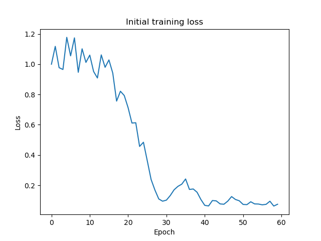
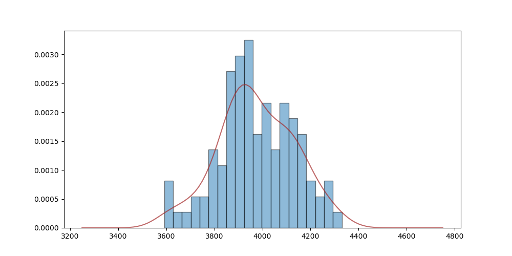
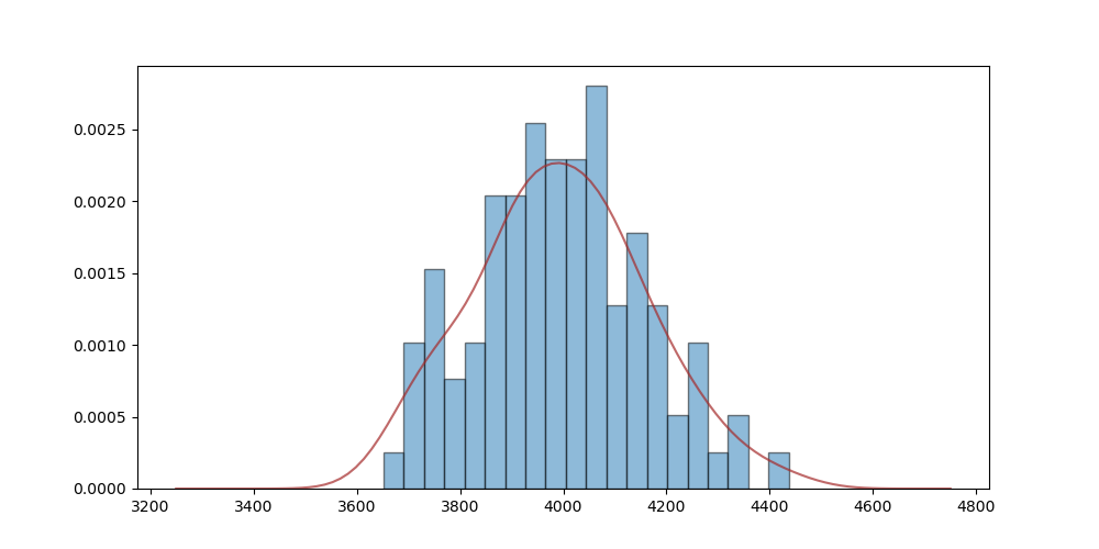
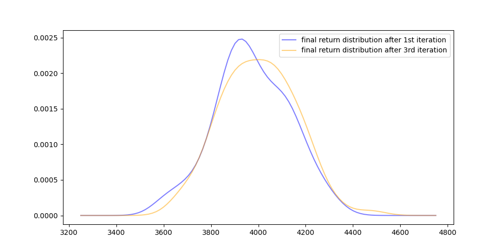
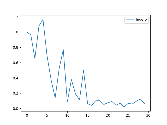
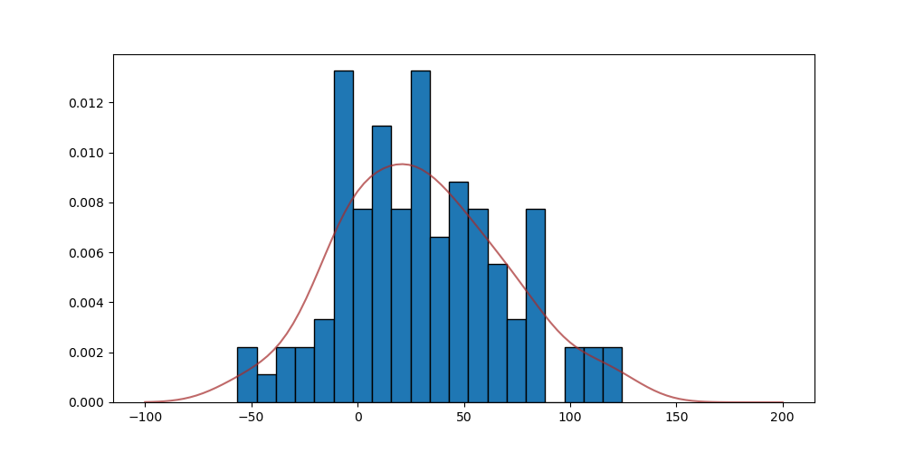
Figure 1 presents the initial loss of the policy improvement algorithm. We iterate the policy update process three times, and Figures 2-4 illustrate the return distributions after each iteration. Each figure showcases a histogram representing the returns obtained from 100 simulations, accompanied by a Gaussian density estimation curve depicting the return distribution. Figure 5 offers a comparison between the Gaussian density estimation after the first policy iteration and the third policy iteration. It is evident that the return distribution after the third policy iteration exhibits a significant improvement over the distribution after the first iteration, indicating enhanced overall performance.

Figure 1: initial loss of policy improvement algorithm

Figure 2: return distributions after 1st iteration

Figure 3: return distribution after 2nd iteration

Figure 4: return distribution after 3rd iteration

Figure 5: comparison between return distribution between 1st and 3rd iterations

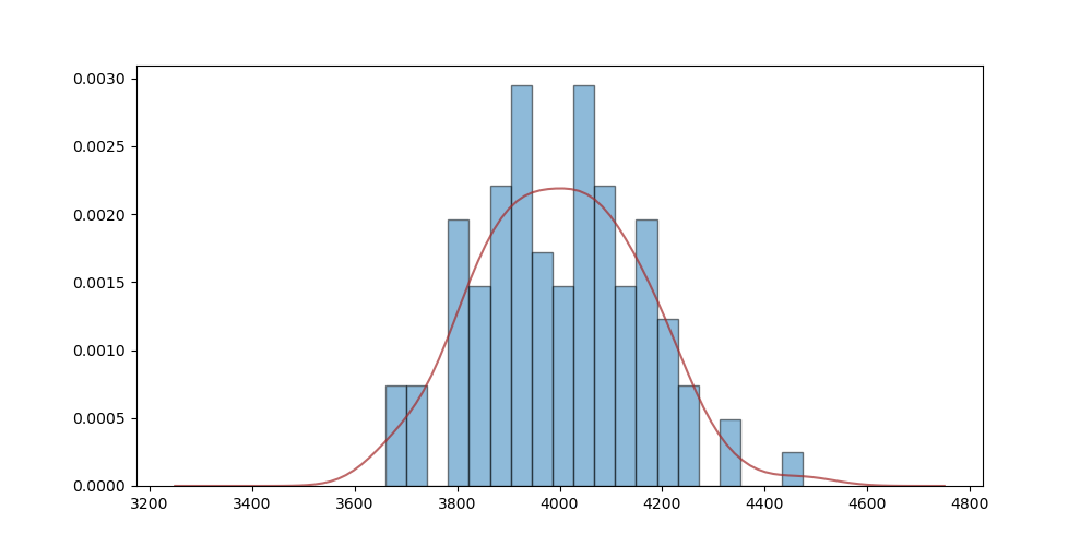
While the return distribution appears favorable, the bid-ask spreads shown in Figures 6-11 exhibit unrealistically large values, which explains why the return distribution reaches thousands of dollars. To illustrate this issue, we provide three examples of posted bid-ask spreads after three policy iterations. Each example corresponds to different time points and inventory configurations.

In the first example, $t=0$, and the inventory $q_{1}$ is given by:

$$q_{1}=\begin{bmatrix}0&0&0&0\\ 0&0&0&0\\ 0&0&0&0\\ 0&0&0&0\\ 0&0&0&0\end{bmatrix}$$

In the second example, $t=0.5$, and the inventory $q_{2}$ is given by:

$$q_{2}=\begin{bmatrix}6&7&8&9\\ 3&4&5&6\\ 0&1&2&3\\ 3&4&5&6\\ 6&7&8&9\end{bmatrix}$$

In the third example, $t=0$, and the inventory $q_{3}$ is given by:

$$q_{3}=\begin{bmatrix}3&4&-5&-6\\ 1&2&-3&-4\\ 0&1&-1&1\\ 1&-2&3&4\\ 2&-3&4&5\end{bmatrix}$$

Despite their unrealistic nature, these bid-ask spreads offer insights into the policy for posting them. The first and most apparent observation is that bid-ask spreads tend to be larger for options with longer maturities, while they are smaller for options with strikes closer to the stock price. Comparing example 1 and example 2, we notice that in example 2, the bid spreads are generally higher for most options, while the ask spreads are lower for most options. This behavior indicates that when there is a positive inventory, our agent adjusts bid-ask spreads to reduce the inventory, aligning with realistic scenarios. If we examine the bid-ask spreads in example 3, we find that options with negative inventories have relatively higher ask spreads. Although these spreads are unrealistic, they provide further insights into the behavior of bid-ask spread policies.

Figure 6: bid spreads example 1

Figure 7: ask spreads example 1

Figure 8: bid spreads example 2

Figure 9: ask spreads example 2

Figure 10: bid spreads example 2

Figure 11: ask spreads example 3

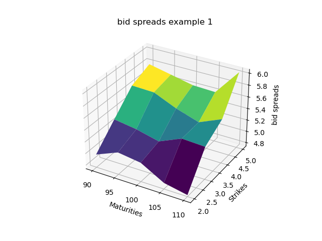
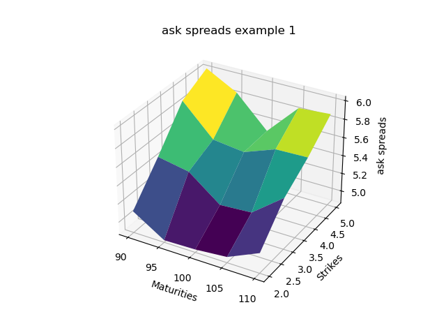
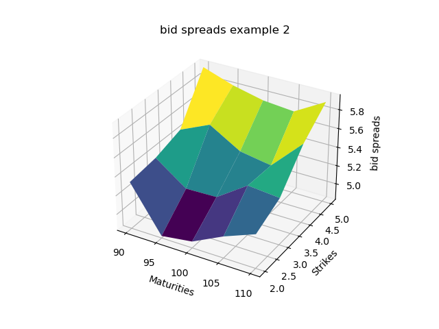
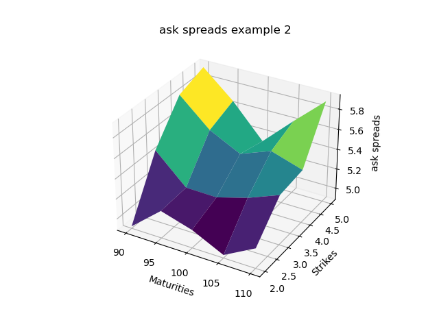
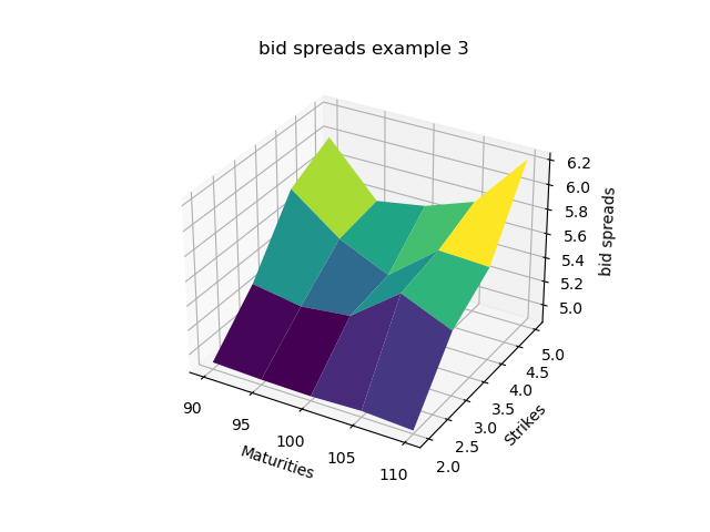
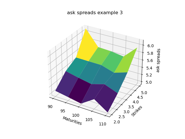
Although the policy improvement algorithm is theoretically sound, the numerical analysis reveals two significant issues. Firstly, due to the assumption made in our setting that the arrival intensity of market orders is linearly inversely related to the bid-ask spreads, the resulting bid-ask spreads become unrealistically large. This assumption leads to a distortion in the spread values, which undermines the realism of our model. Secondly, the choice of neural networks for policy iteration introduces approximation limitations. Without controlling the mean of the policy, there is a possibility that it may become negative, resulting in suboptimal outcomes. These issues highlight the need to address the unrealistic bid-ask spreads and refine the policy control mechanisms for more accurate and reliable results.

Next, we present the results obtained from the actor-critic algorithm. In this algorithm, both the value function and the mean of the Gaussian policy are modeled using the same neural network structure, differing only in the output size for the value function network and the policy mean network. Furthermore, to constrain the range of the proposed bid-ask spreads, we apply a sigmoid activation multiplied by 0.1 to the final output when modeling the mean of the Gaussian policy.

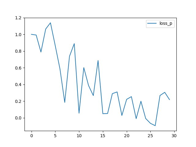
Figures 12-13 depict the loss graphs for the policy loss and critic loss, while figure 14 displays the return distribution, which includes some negative returns but ultimately represents a profitable strategy. These results indicate a more realistic return distribution; however, achieving this comes at the cost of not converging to the optimal strategy due to the imposed limitations on the bid-ask spread range.

Figure 12: p loss

Figure 13: v loss

Figure 14: returns for actor-critic algorithm

7 Conclusion

In this paper, we analyze the market-making problem with the assumption that bid-ask spreads are inversely proportional to the market order arrival intensity. However, it is important to note that this model does not accurately represent real-world conditions, resulting in unrealistic bid-ask spreads. While the bid-ask spreads can be controlled within a reasonable range using the actor-critic algorithm, this introduces a trade-off where the convergence to an optimal policy cannot be guaranteed.

These limitations serve as motivation for further studies on market making in a more realistic setting. We believe that by incorporating more realistic assumptions, the outputs of both algorithms will yield bid-ask spreads that align with each other and the actual market conditions. In such a scenario, the need to incorporate activation functions to control the range of bid-ask spreads within the actor-critic algorithm would no longer be necessary.