Open Quantum System Dynamics from Infinite Tensor Network Contraction

Abstract

Approaching the long-time dynamics of non-Markovian open quantum systems presents a challenging task if the bath is strongly coupled. Recent proposals address this problem through a representation of the so-called process tensor in terms of a tensor network, which can be contracted to matrix product state (MPS) form. We show that for Gaussian environments the stationarity of the bath response can be exploited in order to efficiently construct such a MPS with infinite MPS evolution methods. The result structurally resembles open system evolution with carefully designed auxiliary degrees of freedom, as in hierarchical or pseudomode methods. Here, however, these degrees of freedom are generated automatically by the MPS evolution algorithm. Crucially, the semi-group property of the resulting propagator enables us to reach arbitrary evolution times and apply spectral theory for a systematic exploration of asymptotic properties, such as phase transitions in the steady state. Moreover, our algorithm for contracting the process tensor network leads to significant computational speed-up over existing proposals in the strong coupling regime.

Introduction

Dissipative effects are crucial to our understanding of real world quantum mechanical systems and feature a variety of relevant physical phenomena absent in purely unitary settings. In many realistic and particularly interesting setups, the time scales of system and environment do not separate, leading to a buildup of strong correlations with the environment [1, 2, 3, 4, 5, 6]. Then, advanced numerical tools are required for the simulation of the dynamics on a classical computer [7, 8, 9, 10, 11, 12].

Many of the most sophisticated approaches realize the open system evolution by substituting the original environment with few physical or non-physical auxiliary degrees of freedom. These auxiliary degrees of freedom must be carefully tailored to accurately reproduce the dynamics of the original bath. Prominent methods in this category include the well established HEOM (hierarchical equations of motion) [7] and pseudomode approaches [13, 14, 15], among others [16, 17, 18, 19, 20]. However, identifying suitable auxiliary environments is generally a complex task that depends nontrivially on the specific characteristics of the bath structure [21, 22, 23]. A different strategy to treat open system dynamics avoids this issue by working directly with the exact influence functional [24]. Viewed as a process tensor, it encapsulates all dynamical properties of the reduced dynamics [25]. This tensor has a representation as a two-dimensional tensor network [26, 10, 27, 28], which can be contracted to matrix product state (MPS) form to allow for efficient computations [27, 29, 30, 31, 32, 28].

In this paper we derive an alternative representation of the process tensor in terms of an infinite tensor network. This key result allows us to use infinite time evolving block decimation (iTEBD) [33] for network contraction, leading to a fast algorithm that scales linearly with the bath memory time. The resulting MPS representation of the process tensor has the same structure as for methods using auxiliary degrees of freedom, bridging a gap between the two different approaches. The crucial advantage of this structure is that the complete dynamics is encoded in a single time-local propagator. This not only makes it possible to reach arbitrary evolution times without additional memory requirements, but also to use spectral theory in order to determine stationary states and characterize asymptotic behavior. In contrast to established methods such as HEOM, the auxiliary degrees of freedom are generated automatically in an optimized and systematic way during the network contraction.

Open system evolution

As a model for open system dynamics we consider the standard Hamiltonian

$$H=H_{\mathrm{sys}}(t)\otimes\mathbb{1}_{\mathrm{env}}+S\otimes B(t),$$ (1)

where $H_{\mathrm{sys}}$ and $S$ are hermitian operators in the Hilbert space of the system and $B(t)$ is an operator that describes the collective degrees of freedom of a Gaussian environment consisting of a continuum of bosonic modes [1]. This operator is characterized by the so-called bath correlation function

$$\alpha(t,s)=\mathrm{tr}\,\rho_{\mathrm{env}}(0)B(t)B(s),$$ (2)

where $\rho_{\mathrm{env}}(0)$ is a Gaussian environment initial state . The bath is said to be stationary if the bath correlation function depends only on the time difference $\alpha(t,s)\equiv\alpha(t-s)$. While notable exceptions exist [35], this is the standard scenario in open system dynamics. In order to arrive at a description of the dynamics in terms of the process tensor, we can consider a Trotter splitting of the full unitary time evolution operator [36]

$$U(t+\Delta,t)=U_{\mathrm{sys}}(t+\Delta,t)U_{\mathrm{int}}(t+\Delta,t)+\mathcal{O}(\Delta^{2}),$$ (3)

where $U_{\mathrm{sys}}(t+\Delta,t)$ is the unitary evolution operator generated by $H_{\mathrm{sys}}$ for a time step $\Delta$, and $U_{\mathrm{int}}(t+\Delta,t)$ is the evolution operator generated by the interaction term in (1) . With this splitting the evolution of the reduced system density operator can be decomposed into a part that describes the system evolution, and a part that describes the influence of the bath, the so-called influence functional [38]. Together, these two terms form the process tensor from which all dynamical properties of the system can be extracted [25, 27]. As an example we consider computing the system density matrix after $N$ time steps $t=N\Delta$. We use a Liouville-space (density matrix space) notation where a single index $\mu\equiv(\mu_{l},\mu_{r})$ labels a (‘left’ and ‘right’) pair of eigenstates $|\mu_{l}\rangle$, $|\mu_{r}\rangle$ of the coupling operator $S$, such that matrix elements are denoted by $A^{\mu}=\langle\mu_{l}|A|\mu_{r}\rangle$. Thus, if the dimension of the system Hilbert space is $d$, $\mu$ runs from $1$ to $d^{2}$. The time evolution of the system state is given as [27]

$$\begin{split}&\rho^{\mu_{N}}_{\mathrm{sys}}(N\Delta)=\mathcal{F}_{N}^{\mu_{1}...\mu_{N}}\left(\prod_{k=1}^{N}\mathcal{U}_{\mathrm{sys}}^{\mu_{k},\mu_{k-1}}(k)\right)\rho_{\mathrm{sys}}^{\mu_{0}}(0)\end{split}$$ (4)

with summation implied if indices appear twice. $\mathcal{U}_{\mathrm{sys}}^{\mu,\nu}$ is the unitary channel describing the evolution due to $H_{\mathrm{sys}}$ for a single time step and $\mathcal{F}_{N}$ is the time-discrete influence functional [38], a tensor with $N$ indices. This object fully encapsulates the influence of the system-bath interaction onto the system dynamics and can be used to express the full process tensor. For a stationary Gaussian environment, it has the well known structure [38, 10, 27]

$$\begin{split}&\mathcal{F}_{N}^{\mu_{1}...\mu_{N}}=\prod_{i=1}^{N}\prod_{j=1}^{i}I_{(i-j)}(\mu_{i},\mu_{j})\\ &I_{k}(\mu,\nu)=\exp\left((S_{\mu_{l}}-S_{\mu_{r}})(\eta_{k}S_{\nu_{l}}-\eta_{k}^{*}S_{\nu_{r}})\right),\end{split}$$ (5)

where the discretized bath correlation function is given as

$$\eta_{k}=\begin{cases}\int_{k\Delta}^{(k+1)\Delta}\mathrm{d}t\int_{0}^{\Delta}\mathrm{d}s\,\alpha(t-s),&k>0\\ \int_{0}^{\Delta}\mathrm{d}t\int_{0}^{t}\mathrm{d}s\,\alpha(t-s),&k=0\end{cases}$$ (6)

and $S_{n}$ denotes the $n$’th eigenvalue of the coupling operator. With this exact expression one can in general not directly compute the time evolution according to Eq. (LABEL:eq:time_evo) because this involves a sum over exponentially many terms (exponential in $N$).

Note that using auxiliary degrees of freedom to effectively describe the open system evolution, the time-discrete influence functional takes the MPS form

$$\mathcal{F}_{N}^{\mu_{1}...\mu_{N}}=\vec{v}_{l}^{T}f^{\mu_{1}}f^{\mu_{2}}\cdots f^{\mu_{N}}\vec{v}_{r}$$ (7)

with identical tensors $f$ and two boundary vectors $\vec{v}_{l/r}$. For instance, in the hierarchical equations of motion (HEOM) approach, $f$ is the propagator of the hierarchy for a time step $\Delta$ and the bond dimension is the number of auxiliary density operators [39]. With an MPS form for $\mathcal{F}_{N}$ the open system evolution Eq. (LABEL:eq:time_evo) can be performed with iterative tensor contractions. Our goal is to construct a representation of the type (7) in a way that is systematic and automated, starting from an established network representation of $\mathcal{F}_{N}$.

Tensor Network Representation of the Influence Functional

It has been shown in Refs. [26, 10, 27] that the time-discrete influence functional (5) can be represented as a two-dimensional tensor network. For this one can define a set of tensors

$$b^{\mu\nu}_{ij}(k)=\begin{cases}\delta_{ij}\delta_{\mu\nu}I_{k}(\mu,j),&k>0\\ \delta_{ij}\delta_{\mu\nu}\delta_{j\mu}I_{0}(\mu,j),&k=0\end{cases}=\vbox{\includegraphics{ main-figure0.pdf}}\,.$$ (8)

Then the influence functional is given by the network depicted in Fig. 1. In the PT-TEMPO scheme (Process Tensor Time Evolving Matrix Product Operators) [10, 27, 29, 40], this network is iteratively contracted to a matrix product state by multiplying adjacent columns followed by SVD compression which is required to keep the bond dimension manageable. This compression step is the demanding operation in the algorithm. At first sight, to compute a process tensor for $N$ time steps, $\mathcal{O}(N^{2})$ singular value decompositions are required to contract the network. However, usually one assumes a finite memory time of the bath such that all $b(k)$ tensors for $k>N_{c}$ can be neglected . Then, using advanced algorithms, the scaling of the network contraction can be improved to $\mathcal{O}(N_{c}\log N_{c})$ [42]. These contraction methods based on finite MPS evolution do not deliver a periodic representation with a single time step propagator as in Eq. (7). In the following we derive a new method that achieves this form and requires exactly $N_{c}$ singular value decompositions.

Figure 1: Representation of the time discrete influence functional $\mathcal{F}_{N}$ as a tensor network for $N=5$ [10, 27]. In order to efficiently compute open system dynamics, this network has to be contracted to matrix product state form with small bond dimension (red tensors). Tensor legs that are not drawn have to be summed over.

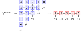
For the new scheme that we propose the network has to be modified slightly. We extend the index dimension ($d^{2}$) of the tensors $b(k)$ by one, introducing a ‘zero’ dimension via $I_{k}(0,i)=I_{k}(i,0)\equiv 1$, and keeping the definition (8) as is. This does not have a significant effect on the complexity of the network. If one index of an extended $b(k)$ tensor is zero, the tensor reduces to a trivial product of delta functions. As demonstrated in the supplementary material [39], this property allows us to obtain the influence functional for $M<N$ time steps from the influence functional for $N$ time steps by inserting zeros at the boundary

$$\mathcal{F}_{M}^{\mu_{1}...\mu_{M}}=\mathcal{F}_{N}^{0...0,\mu_{1}...\mu_{M}}=\mathcal{F}_{N}^{\mu_{1}...\mu_{M},0...0}.$$ (9)

We can even factor the influence functional into two by piercing the train of indices with at least $N_{c}$ zeros

$$\mathcal{F}^{\mu_{1}...\mu_{M},0...0,\nu_{1}...\nu_{K}}_{N}=\mathcal{F}_{M}^{\mu_{1}...\mu_{M}}\mathcal{F}_{K}^{\nu_{1}...\nu_{K}}.$$ (10)

This suggests the following strategy to compute $\mathcal{F}^{\mu_{1}...\mu_{N}}_{N}$. We compute an influence functional with periodic boundary condition in the infinite time-step limit in the form

$$\mathcal{F}^{...\mu\nu\delta...}_{\infty}=\mathrm{tr}\left[\cdots f^{\mu}f^{\nu}f^{\delta}\cdots\right]$$ (11)

where $f^{\mu}$ are $\chi\times\chi$ matrices (bond dimension $\chi$, $\mu=0,1,...,d^{2}$). We can then obtain the desired influence functional for $N$ steps via

$$\mathcal{F}_{N}^{\mu_{1}...\mu_{N}}=\mathrm{tr}\left[(f^{0})^{\gamma}f^{\mu_{1}}f^{\mu_{2}}\cdots f^{\mu_{N}}\right],$$ (12)

where $\gamma\geq N_{c}$. In practice, one can set $\gamma=\infty$ such that $(f^{0})^{\gamma}=\vec{v}_{r}\circ\vec{v}_{l}$ with $\vec{v}_{l/r}$ the leading left and right eigenvectors of $f^{0}$ (eigenvalue one). We have indeed recovered a representation of the type (7). Therefore, one only needs to compute and store the single tensor $f$ instead of $\mathcal{O}(N_{c})$ such tensors as in the finite contraction schemes [42]. As demonstrated in the supplementary material, the stationary state can also be determined efficiently by computing the leading eigenvector of the full short-time propagator $\mathcal{Q}_{(\mu,i)}^{(\nu,j)}=f^{\mu}_{ij}\mathcal{U}_{\mathrm{sys}}^{\mu,\nu}$ [39].

Algorithm

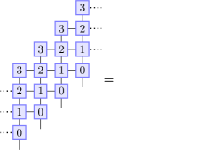
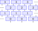
In order to find the tensor $f$ of the infinite network we propose a contraction in an ‘anti-diagonal’ direction starting from $k=N_{c}$, as shown in Fig. 2, when the network displays a structure suitable for time evolving block decimation (TEBD). The ‘gates’ $b(k)$ can formally be seen as nearest neighbor coupling alternating between left and right ‘sites’. Thus, it is straightforward to apply infinite TEBD algorithms [33, 43, 44] with MPS evolution from top to bottom (Fig. 2 right panel). Since the gates $b(k)$ are only weakly entangling for large $k$, the bond dimension increases significantly only for the last few evolution steps, making this an excellent contraction scheme. The simple iTEBD algorithm from Ref. [43] already performs very well, resulting in similar bond dimension for a given accuracy as the contraction of the finite network, but with a computational speedup in orders of magnitude (for more details of this computational advantage see the supplemental material [39]).

Figure 2: Visual representation of an infinite influence functional with $N_{c}=3$ as nearest-neighbor matrix product state evolution.

Applications

For the following examples we consider a (sub-)ohmic bath with exponential cutoff. At zero temperature the bath correlation function reads [9]

$$\alpha(t)=\alpha\omega_{c}^{2}\frac{\Gamma(s+1)}{2(1+\mathrm{i}\omega_{c}t)^{s+1}}.$$ (13)

In this expression, $\alpha$ is a dimensionless coupling strength, $\omega_{c}$ is the cutoff frequency, and $s\leq 1$ is the exponent of the low frequency behavior $\propto\omega^{s}$ of the spectral density. This function decays algebraically for large times, possibly making it challenging for simulations due to a resulting long memory time.

As a first example we compute the asymptotic entanglement in a two-spin boson model. The model consists of noninteracting spins $A$ and $B$ that are coupled to the same bath via

$$H(t)=\frac{\Omega}{2}(\sigma_{x}^{A}+\sigma_{x}^{B})\otimes\mathbb{1}_{\mathrm{env}}+\frac{1}{2}\left(\sigma_{z}^{A}+\sigma_{z}^{B}\right)\otimes B(t).$$ (14)

Even if the spins are not directly coupled, at low temperatures, they still become entangled via the interaction with a common bath [45]. A crucial advantage of our framework is that we can use a spectral decomposition of $\mathcal{Q}$ to determine the steady state without relying on time evolution [46, 47]. This allows us to effortlessly obtain accurate values for the asymptotic concurrence over large parameter regimes, displayed in Fig. 3. As can be expected, the concurrence increases with the coupling strength and decreases with temperature. For every coupling strength a maximum temperature exists after which the asymptotic state becomes separable. Note that even for weak coupling the concurrence is difficult to compute using standard perturbative master equations. As shown in Fig. 3, the second order Redfield equation [48] predicts systematically wrong values for weak coupling. In fact, second order master equations predict the steady state only to zeroth order accuracy [49, 45], while obtaining higher order equations is tedious [50].

Figure 3: Steady state concurrence in the two-spin boson model with an ohmic bath ($s=1$, $\omega_{c}=5\Omega$) for different coupling strengths and temperatures. The lower panel shows cuts for the coupling strengths indicated by the lines in the upper panel. As a comparison, the concurrence predicted by Redfield theory is displayed as dashed lines.

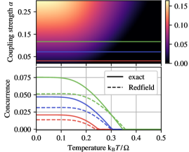
We further exemplify the power of a spectral analysis by studying the well-known quantum phase transition in the sub-Ohmic spin boson model [51, 52, 53, 23]

$$H(t)=\Omega\sigma_{x}\otimes\mathbb{1}_{\mathrm{env}}+\sigma_{z}\otimes B(t).$$ (15)

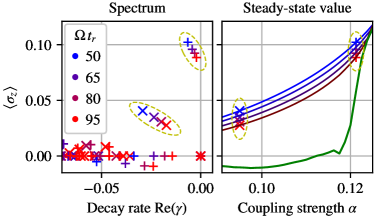
As the coupling strength $\alpha$ is increased, the system changes from a symmetric phase, where asymptotically $\langle\sigma_{z}\rangle=0$, to a symmetry broken phase $\langle\sigma_{z}\rangle\neq 0$. In general, such phase transitions are difficult to describe via time evolution because it is hard to separate asymptotic and transient behavior, especially since numerical approaches will typically generate a gapped spectrum [10, 54]. In our framework we can employ a spectral decomposition in order to write the evolution of any observable as

$$\langle\sigma_{z}\rangle(t)=\sum_{k=1}^{\chi d^{2}}\mathrm{e}^{\gamma_{k}t}\langle\sigma_{z}\rangle_{k},$$ (16)

where $\gamma_{k}$ are complex rates extracted from the eigenvalues of the short time propagator $\mathcal{Q}$. For large $t$ we can keep only the two most relevant contributions in the sum, the leading and next-to-leading eigenvector

$$\langle\sigma_{z}\rangle(t)\rightarrow\mathrm{e}^{\gamma_{1}t}\langle\sigma_{z}\rangle_{1}+\mathrm{e}^{\gamma_{2}t}\langle\sigma_{z}\rangle_{2}.$$ (17)

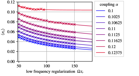
For the spin boson model this requires further justification, because the exact spectrum is not gapped. We provide a full discussion of the subtleties in the supplement [39]. There always exists a unique steady state contribution with $\gamma_{1}=0$ which obeys the symmetry of the model $\langle\sigma_{z}\rangle_{1}=0$. Hence, to describe the transition, we must consider the next-to-leading eigenvector. In order to ensure convergence of the algorithm, we modify the bath correlation function after a time $t_{r}$ to decay exponentially (low frequency regularization). The original spin boson model is recovered when $t_{r}\rightarrow\infty$. In this limit we find for all coupling strengths that $\gamma_{2}\rightarrow 0$ (see Fig. 4). Thus, the symmetry breaking is characterized by the value of $\langle\sigma_{z}\rangle_{2}$ extrapolated to large $t_{r}$. Since the phase transition is second order, we make an extrapolation by fitting algebraic curves to the numerical data. The results are displayed in Fig. 4. While the finite $t_{r}$ curves (red and blue) do not indicate the transition point, we can clearly identify the critical coupling from the extrapolated values (green curve).

Figure 4: Predictions for the stationary $\sigma_{z}$ expectation value in the sub-ohmic spin boson model ($s=0.5$, $\omega_{c}=20\Omega$) using different low frequency regularizations $t_{r}$. The left panel shows the spectral contributions to $\sigma_{z}$ from the numerically computed short time propagator above and below the transition. We can identify the unique steady state ($\gamma=0$, $\langle\sigma_{z}\rangle=0$) as well as the next-to-leading contribution which breaks the symmetry (encircled). On the right hand side the predicted steady state values are displayed as a function of the coupling strength. The green line shows the extrapolated values from algebraic fits [39]. We can identify the phase transition at $\alpha\approx 0.1175$.

Conclusions

We have introduced a new method to automatically generate auxiliary environments for simulations of open quantum system dynamics. These degrees of freedom realize the exact bath response to a controlled level of accuracy and with a time-local propagator. Our approach is based on an established tensor network representation of the process tensor [10, 27, 29]. This network can be modified such that the contraction to MPS form can be performed using infinite MPS evolution methods. As suggested from the network structure, we use iTEBD, resulting in a linear scaling of the computation effort with the bath memory time (i.e. linear in $N_{c}$). The resulting influence functional is represented in terms of a single tensor $f$, with insignificant memory requirements in comparison with the finite network contraction algorithms, which require to store at least $N_{c}$ tensors . This tensor encodes both propagator and initial state for a set of auxiliary degrees of freedom. Since such a representation is time-local, the open system evolution can be trivially extended to arbitrary long times and stationary states can be determined efficiently using power methods. Furthermore, we can utilize a spectral decomposition in order to characterize asymptotic behavior and dissipative phase transitions. Our proposed algorithm constitutes a powerful method for open quantum systems that is simple to implement and that can be used readily for any stationary Gaussian environment. Still, we believe there is substantial potential for further optimization. For instance, using advanced infinite MPS evolution schemes [56, 57, 58] could lead to a better accuracy at a given bond dimension, which becomes relevant for large system sizes and ultra strong coupling.

Acknowledgements

V.L. and W.T.S. gratefully acknowledge discussions with Richard Hartmann concerning the numerical examples. We also thank Jonathan Keeling for valuable comments on a previous version of the manuscript. H.-H.T. is supported by the Deutsche Forschungsgemeinschaft (DFG) through project A06 of SFB 1143 (project No. 247310070).

Supplementary Material

.1 A. MPS representation of the influence functional from HEOM

We show how Eq. (7) can be obtained from open system dynamics with auxiliary environments, considering HEOM as an example [7]. In the standard HEOM scheme, the bath correlation function is represented approximately as a sum over few exponentials, [23]

$$\alpha(t)\approx\sum_{j=1}^{M}G_{j}\mathrm{e}^{-\mathrm{Re}W_{j}|t|-\mathrm{i}\mathrm{Im}W_{j}t},$$ (S1)

with complex parameters $G_{j},W_{j}\in\mathbb{C}$. One then defines an infinite set of auxiliary density operators labeled by a pair of multiindices $\boldsymbol{n},\boldsymbol{m}\in\mathbb{N}_{0}^{M}$. These auxiliary states satisfy the hierarchical equation of motion

$$\begin{split}\partial_{t}\rho^{(\boldsymbol{n},\boldsymbol{m})}=&-i[H_{\mathrm{sys}},\rho^{(\boldsymbol{n},\boldsymbol{m})}]-\left(\boldsymbol{W}\cdot\boldsymbol{n}+\boldsymbol{W}^{*}\cdot\boldsymbol{m}\right)\rho^{(\boldsymbol{n},\boldsymbol{m})}+\sum_{j}\left(G_{j}n_{j}S\rho^{(\boldsymbol{n}-\boldsymbol{e}_{j},\boldsymbol{m})}+G_{j}^{*}m_{j}\rho^{(\boldsymbol{n},\boldsymbol{m}-\boldsymbol{e}_{j})}S\right)\\ &+\sum_{j}\left[\rho^{(\boldsymbol{n}+\boldsymbol{e}_{j},\boldsymbol{m})},S\right]+\left[S,\rho^{(\boldsymbol{n},\boldsymbol{m}+\boldsymbol{e}_{j})}\right]\!.\end{split}$$ (S2)

We denote $\boldsymbol{e}_{i}$ the unit vector in direction $i$. Choosing as an initial state $\rho^{(\boldsymbol{0},\boldsymbol{0})}(0)=\rho(0)$ and all other states zero, one can obtain the reduced system evolution from $\rho(t)=\rho^{(\boldsymbol{0},\boldsymbol{0})}(t)$. In practice, the hierarchy is cut at sufficiently high index values such that a finite system can be evolved numerically. We can reformulate the hierarchy by embedding it as an operator in an extended Hilbertspace $\rho^{(\boldsymbol{n},\boldsymbol{m})}\equiv\langle\boldsymbol{n}|R|\boldsymbol{m}\rangle$ [20, 60]. Defining raising and lowering operators $A_{i}^{\pm}|\boldsymbol{n}\rangle=|\boldsymbol{n}\pm\boldsymbol{e}_{i}\rangle$, and counting operators $N_{i}|\boldsymbol{n}\rangle=n_{i}|\boldsymbol{n}\rangle$ the hierarchy is mapped onto

$$\begin{split}\partial_{t}R&=-i[H_{\mathrm{sys}},R]-\left(\boldsymbol{W}\cdot\boldsymbol{N}R+R\boldsymbol{W}^{*}\cdot\boldsymbol{N}\right)+\sum_{j}\left(G_{j}A^{+}_{j}N_{j}SR+G_{j}^{*}RSN_{j}A^{-}_{j}\right)+\sum_{j}\big{(}\left[A^{-}_{j}R,S\right]+\left[S,RA^{+}_{j}\right]\big{)}\\ &\equiv\mathcal{L}_{\mathrm{sys}}R+\mathcal{L}_{\mathrm{int}}R\,.\end{split}$$ (S3)

Since the evolution is linear we can employ a Trotter splitting with time step $\Delta$ between $\mathcal{L}_{\mathrm{sys}}=-\mathrm{i}[H_{\mathrm{sys}},\cdot]$ and $\mathcal{L}_{\mathrm{int}}$. $\mathcal{L}_{\mathrm{int}}$ commutes with the coupling operator $S$, so we consider the action of this generator on a product of $S$-eigenstates $|\mu_{l}\rangle\!\langle\mu_{r}|$ labeled with the index $\mu=(\mu_{l},\mu_{r})$

$$\mathcal{L}_{\mathrm{int}}\left(|\mu_{l}\rangle\!\langle\mu_{r}|\otimes x\right)=|\mu_{l}\rangle\!\langle\mu_{r}|\otimes\mathcal{L}_{\mathrm{int}}^{\mu}x.$$ (S4)

The generator of the hierarchy dynamics conditioned on the system basis state is given as

$$\mathcal{L}_{\mathrm{int}}^{\mu}x=-\left(\boldsymbol{W}\cdot\boldsymbol{N}x+x\boldsymbol{W}^{*}\cdot\boldsymbol{N}\right)+\sum_{j}\left(G_{j}A^{+}_{j}N_{j}S_{\mu_{l}}x+G_{j}^{*}xS_{\mu_{r}}N_{j}A^{-}_{j}\right)+\sum_{j}\big{(}A^{-}_{j}x(S_{\mu_{r}}-S_{\mu_{l}})+(S_{\mu_{l}}-S_{\mu_{r}})xA^{+}_{j}\big{)}.$$ (S5)

The tensor $f^{\mu}$ is just the propagator generated by $\mathcal{L}_{\mathrm{int}}^{\mu}$ for a time step $\Delta$

$$f^{\mu}=\mathrm{e}^{\Delta\mathcal{L}_{\mathrm{int}}^{\mu}}.$$ (S6)

The bond dimension of $f$ is exactly the number of auxiliary density operators that are taken into account in the hierarchy. We obtain an influence functional of the form (7) with the boundary vectors $v_{l}=v_{r}=|\boldsymbol{0}\rangle\!\langle\boldsymbol{0}|$ (the system state is given by $\rho=\langle\boldsymbol{0}|R|\boldsymbol{0}\rangle$).

.2 B. Reduction of the influence functional

We provide a proof for the statements (9) and (10). These allow us to recover the influence functional for finite times from the infinite version. From our definition, the extended tensors $b(k)$ have the property that, if one index is zero, they reduce to a product of delta functions. In particular

$$b^{0\nu}_{ij}(k)=\begin{cases}\delta_{ij}\delta_{0\nu},&k>0\\ \delta_{ij}\delta_{0\nu}\delta_{j0},&k=0\end{cases}\,,\qquad b^{\mu\nu}_{0j}(k)=\begin{cases}\delta_{0j}\delta_{\mu\nu},&k>0\\ \delta_{0j}\delta_{\mu\nu}\delta_{j\mu},&k=0\end{cases}\,.$$ (S7)

We write this as

$$b^{\mu\nu}_{0j}(k>0)=\vbox{ \leavevmode\hbox to50.37pt{\vbox to50.8pt{\pgfpicture\makeatletter\hbox{\hskip 25.10745pt\lower-25.88719pt\hbox to0.0pt{\pgfsys@beginscope\pgfsys@invoke{ }\definecolor{pgfstrokecolor}{rgb}{0,0,0}\pgfsys@color@rgb@stroke{0}{0}{0}\pgfsys@invoke{ }\pgfsys@color@rgb@fill{0}{0}{0}\pgfsys@invoke{ }\pgfsys@setlinewidth{0.4pt}\pgfsys@invoke{ }\nullfont\hbox to0.0pt{\pgfsys@beginscope\pgfsys@invoke{ }{}{} {{}}\hbox{\hbox{{\pgfsys@beginscope\pgfsys@invoke{ }{{}{}{{ {}{}}}{ {}{}} {{}{{}}}{{}{}}{}{{}{}} { }{{{{}}\pgfsys@beginscope\pgfsys@invoke{ }\pgfsys@transformcm{1.0}{0.0}{0.0}{1.0}{-2.46991pt}{17.76416pt}\pgfsys@invoke{ }\hbox{{\definecolor{pgfstrokecolor}{rgb}{0,0,0}\pgfsys@color@rgb@stroke{0}{0}{0}\pgfsys@invoke{ }\pgfsys@color@rgb@fill{0}{0}{0}\pgfsys@invoke{ }\hbox{{$\nu$}} }}\pgfsys@invoke{\lxSVG@closescope }\pgfsys@endscope}}} \pgfsys@invoke{\lxSVG@closescope }\pgfsys@endscope}}} {}{{}}{}{ {}{}{}} {{{{{}}{ {}{}}{}{}{{}{}}}}}{}{}{}{}\pgfsys@moveto{0.0pt}{0.0pt}\pgfsys@lineto{0.0pt}{14.71889pt}\pgfsys@stroke\pgfsys@invoke{ } {{}}\hbox{\hbox{{\pgfsys@beginscope\pgfsys@invoke{ }{{}{}{{ {}{}}}{ {}{}} {{}{{}}}{{}{}}{}{{}{}} { }{{{{}}\pgfsys@beginscope\pgfsys@invoke{ }\pgfsys@transformcm{1.0}{0.0}{0.0}{1.0}{-3.01274pt}{-21.09749pt}\pgfsys@invoke{ }\hbox{{\definecolor{pgfstrokecolor}{rgb}{0,0,0}\pgfsys@color@rgb@stroke{0}{0}{0}\pgfsys@invoke{ }\pgfsys@color@rgb@fill{0}{0}{0}\pgfsys@invoke{ }\hbox{{$\mu$}} }}\pgfsys@invoke{\lxSVG@closescope }\pgfsys@endscope}}} \pgfsys@invoke{\lxSVG@closescope }\pgfsys@endscope}}} {}{{}}{}{ {}{}{}} {{{{{}}{ {}{}}{}{}{{}{}}}}}{}{}{}{}\pgfsys@moveto{0.0pt}{0.0pt}\pgfsys@lineto{0.0pt}{-13.74667pt}\pgfsys@stroke\pgfsys@invoke{ } {{}}\hbox{\hbox{{\pgfsys@beginscope\pgfsys@invoke{ }{{}{}{{ {}{}}}{ {}{}} {{}{{}}}{{}{}}{}{{}{}} { }{{{{}}\pgfsys@beginscope\pgfsys@invoke{ }\pgfsys@transformcm{1.0}{0.0}{0.0}{1.0}{-22.26218pt}{-2.32541pt}\pgfsys@invoke{ }\hbox{{\definecolor{pgfstrokecolor}{rgb}{0,0,0}\pgfsys@color@rgb@stroke{0}{0}{0}\pgfsys@invoke{ }\pgfsys@color@rgb@fill{0}{0}{0}\pgfsys@invoke{ }\hbox{{$j$}} }}\pgfsys@invoke{\lxSVG@closescope }\pgfsys@endscope}}} \pgfsys@invoke{\lxSVG@closescope }\pgfsys@endscope}}} {}{{}}{}{ {}{}{}} {{{{{}}{ {}{}}{}{}{{}{}}}}}{}{}{}{}\pgfsys@moveto{-1.9918pt}{0.0pt}\pgfsys@lineto{-14.52641pt}{0.0pt}\pgfsys@stroke\pgfsys@invoke{ } {{}}\hbox{\hbox{{\pgfsys@beginscope\pgfsys@invoke{ }{{}{}{{ {}{}}}{ {}{}} {{}{{}}}{{}{}}{}{{}{}} { }{{{{}}\pgfsys@beginscope\pgfsys@invoke{ }\pgfsys@transformcm{1.0}{0.0}{0.0}{1.0}{17.41693pt}{-3.22221pt}\pgfsys@invoke{ }\hbox{{\definecolor{pgfstrokecolor}{rgb}{0,0,0}\pgfsys@color@rgb@stroke{0}{0}{0}\pgfsys@invoke{ }\pgfsys@color@rgb@fill{0}{0}{0}\pgfsys@invoke{ }\hbox{{$0$}} }}\pgfsys@invoke{\lxSVG@closescope }\pgfsys@endscope}}} \pgfsys@invoke{\lxSVG@closescope }\pgfsys@endscope}}} {}{{}}{}{ {}{}{}} {{{{{}}{ {}{}}{}{}{{}{}}}}}{}{}{}{}\pgfsys@moveto{1.9918pt}{0.0pt}\pgfsys@lineto{14.37166pt}{0.0pt}\pgfsys@stroke\pgfsys@invoke{ } \pgfsys@invoke{\lxSVG@closescope }\pgfsys@endscope{}{}{}\hss}\pgfsys@discardpath\pgfsys@invoke{\lxSVG@closescope }\pgfsys@endscope\hss}}\lxSVG@closescope\endpgfpicture}}}\qquad b^{0\nu}_{ij}(k>0)=\vbox{ \leavevmode\hbox to49.59pt{\vbox to50.9pt{\pgfpicture\makeatletter\hbox{\hskip 25.10745pt\lower-25.98442pt\hbox to0.0pt{\pgfsys@beginscope\pgfsys@invoke{ }\definecolor{pgfstrokecolor}{rgb}{0,0,0}\pgfsys@color@rgb@stroke{0}{0}{0}\pgfsys@invoke{ }\pgfsys@color@rgb@fill{0}{0}{0}\pgfsys@invoke{ }\pgfsys@setlinewidth{0.4pt}\pgfsys@invoke{ }\nullfont\hbox to0.0pt{\pgfsys@beginscope\pgfsys@invoke{ }{}{} {{}}\hbox{\hbox{{\pgfsys@beginscope\pgfsys@invoke{ }{{}{}{{ {}{}}}{ {}{}} {{}{{}}}{{}{}}{}{{}{}} { }{{{{}}\pgfsys@beginscope\pgfsys@invoke{ }\pgfsys@transformcm{1.0}{0.0}{0.0}{1.0}{-2.46991pt}{17.76416pt}\pgfsys@invoke{ }\hbox{{\definecolor{pgfstrokecolor}{rgb}{0,0,0}\pgfsys@color@rgb@stroke{0}{0}{0}\pgfsys@invoke{ }\pgfsys@color@rgb@fill{0}{0}{0}\pgfsys@invoke{ }\hbox{{$\nu$}} }}\pgfsys@invoke{\lxSVG@closescope }\pgfsys@endscope}}} \pgfsys@invoke{\lxSVG@closescope }\pgfsys@endscope}}} {}{{}}{}{ {}{}{}} {{{{{}}{ {}{}}{}{}{{}{}}}}}{}{}{}{}\pgfsys@moveto{0.0pt}{0.0pt}\pgfsys@lineto{0.0pt}{14.71889pt}\pgfsys@stroke\pgfsys@invoke{ } {{}}\hbox{\hbox{{\pgfsys@beginscope\pgfsys@invoke{ }{{}{}{{ {}{}}}{ {}{}} {{}{{}}}{{}{}}{}{{}{}} { }{{{{}}\pgfsys@beginscope\pgfsys@invoke{ }\pgfsys@transformcm{1.0}{0.0}{0.0}{1.0}{-2.5pt}{-23.13914pt}\pgfsys@invoke{ }\hbox{{\definecolor{pgfstrokecolor}{rgb}{0,0,0}\pgfsys@color@rgb@stroke{0}{0}{0}\pgfsys@invoke{ }\pgfsys@color@rgb@fill{0}{0}{0}\pgfsys@invoke{ }\hbox{{$0$}} }}\pgfsys@invoke{\lxSVG@closescope }\pgfsys@endscope}}} \pgfsys@invoke{\lxSVG@closescope }\pgfsys@endscope}}} {}{{}}{}{ {}{}{}} {{{{{}}{ {}{}}{}{}{{}{}}}}}{}{}{}{}\pgfsys@moveto{0.0pt}{0.0pt}\pgfsys@lineto{0.0pt}{-13.64944pt}\pgfsys@stroke\pgfsys@invoke{ } {{}}\hbox{\hbox{{\pgfsys@beginscope\pgfsys@invoke{ }{{}{}{{ {}{}}}{ {}{}} {{}{{}}}{{}{}}{}{{}{}} { }{{{{}}\pgfsys@beginscope\pgfsys@invoke{ }\pgfsys@transformcm{1.0}{0.0}{0.0}{1.0}{-22.26218pt}{-2.32541pt}\pgfsys@invoke{ }\hbox{{\definecolor{pgfstrokecolor}{rgb}{0,0,0}\pgfsys@color@rgb@stroke{0}{0}{0}\pgfsys@invoke{ }\pgfsys@color@rgb@fill{0}{0}{0}\pgfsys@invoke{ }\hbox{{$j$}} }}\pgfsys@invoke{\lxSVG@closescope }\pgfsys@endscope}}} \pgfsys@invoke{\lxSVG@closescope }\pgfsys@endscope}}} {}{{}}{}{ {}{}{}} {{{{{}}{ {}{}}{}{}{{}{}}}}}{}{}{}{}\pgfsys@moveto{-1.9918pt}{0.0pt}\pgfsys@lineto{-14.52641pt}{0.0pt}\pgfsys@stroke\pgfsys@invoke{ } {{}}\hbox{\hbox{{\pgfsys@beginscope\pgfsys@invoke{ }{{}{}{{ {}{}}}{ {}{}} {{}{{}}}{{}{}}{}{{}{}} { }{{{{}}\pgfsys@beginscope\pgfsys@invoke{ }\pgfsys@transformcm{1.0}{0.0}{0.0}{1.0}{18.19437pt}{-3.29762pt}\pgfsys@invoke{ }\hbox{{\definecolor{pgfstrokecolor}{rgb}{0,0,0}\pgfsys@color@rgb@stroke{0}{0}{0}\pgfsys@invoke{ }\pgfsys@color@rgb@fill{0}{0}{0}\pgfsys@invoke{ }\hbox{{$i$}} }}\pgfsys@invoke{\lxSVG@closescope }\pgfsys@endscope}}} \pgfsys@invoke{\lxSVG@closescope }\pgfsys@endscope}}} {}{{}}{}{ {}{}{}} {{{{{}}{ {}{}}{}{}{{}{}}}}}{}{}{}{}\pgfsys@moveto{1.9918pt}{0.0pt}\pgfsys@lineto{15.1491pt}{0.0pt}\pgfsys@stroke\pgfsys@invoke{ } \pgfsys@invoke{\lxSVG@closescope }\pgfsys@endscope{}{}{}\hss}\pgfsys@discardpath\pgfsys@invoke{\lxSVG@closescope }\pgfsys@endscope\hss}}\lxSVG@closescope\endpgfpicture}}}\qquad b^{0\nu}_{ij}(0)=\vbox{ \leavevmode\hbox to49.59pt{\vbox to50.9pt{\pgfpicture\makeatletter\hbox{\hskip 25.10745pt\lower-25.98442pt\hbox to0.0pt{\pgfsys@beginscope\pgfsys@invoke{ }\definecolor{pgfstrokecolor}{rgb}{0,0,0}\pgfsys@color@rgb@stroke{0}{0}{0}\pgfsys@invoke{ }\pgfsys@color@rgb@fill{0}{0}{0}\pgfsys@invoke{ }\pgfsys@setlinewidth{0.4pt}\pgfsys@invoke{ }\nullfont\hbox to0.0pt{\pgfsys@beginscope\pgfsys@invoke{ }{}{} {{}}\hbox{\hbox{{\pgfsys@beginscope\pgfsys@invoke{ }{{}{}{{ {}{}}}{ {}{}} {{}{{}}}{{}{}}{}{{}{}} { }{{{{}}\pgfsys@beginscope\pgfsys@invoke{ }\pgfsys@transformcm{1.0}{0.0}{0.0}{1.0}{-2.46991pt}{17.76416pt}\pgfsys@invoke{ }\hbox{{\definecolor{pgfstrokecolor}{rgb}{0,0,0}\pgfsys@color@rgb@stroke{0}{0}{0}\pgfsys@invoke{ }\pgfsys@color@rgb@fill{0}{0}{0}\pgfsys@invoke{ }\hbox{{$\nu$}} }}\pgfsys@invoke{\lxSVG@closescope }\pgfsys@endscope}}} \pgfsys@invoke{\lxSVG@closescope }\pgfsys@endscope}}} {}{{}}{}{ {}{}{}} {{{{{}}{ {}{}}{}{}{{}{}}}}}{}{}{}{}\pgfsys@moveto{0.0pt}{0.0pt}\pgfsys@lineto{0.0pt}{14.71889pt}\pgfsys@stroke\pgfsys@invoke{ } {{}}\hbox{\hbox{{\pgfsys@beginscope\pgfsys@invoke{ }{{}{}{{ {}{}}}{ {}{}} {{}{{}}}{{}{}}{}{{}{}} { }{{{{}}\pgfsys@beginscope\pgfsys@invoke{ }\pgfsys@transformcm{1.0}{0.0}{0.0}{1.0}{-2.5pt}{-23.13914pt}\pgfsys@invoke{ }\hbox{{\definecolor{pgfstrokecolor}{rgb}{0,0,0}\pgfsys@color@rgb@stroke{0}{0}{0}\pgfsys@invoke{ }\pgfsys@color@rgb@fill{0}{0}{0}\pgfsys@invoke{ }\hbox{{$0$}} }}\pgfsys@invoke{\lxSVG@closescope }\pgfsys@endscope}}} \pgfsys@invoke{\lxSVG@closescope }\pgfsys@endscope}}} {}{{}}{}{ {}{}{}} {{{{{}}{ {}{}}{}{}{{}{}}}}}{}{}{}{}\pgfsys@moveto{0.0pt}{0.0pt}\pgfsys@lineto{0.0pt}{-13.64944pt}\pgfsys@stroke\pgfsys@invoke{ } {{}}\hbox{\hbox{{\pgfsys@beginscope\pgfsys@invoke{ }{{}{}{{ {}{}}}{ {}{}} {{}{{}}}{{}{}}{}{{}{}} { }{{{{}}\pgfsys@beginscope\pgfsys@invoke{ }\pgfsys@transformcm{1.0}{0.0}{0.0}{1.0}{-22.26218pt}{-2.32541pt}\pgfsys@invoke{ }\hbox{{\definecolor{pgfstrokecolor}{rgb}{0,0,0}\pgfsys@color@rgb@stroke{0}{0}{0}\pgfsys@invoke{ }\pgfsys@color@rgb@fill{0}{0}{0}\pgfsys@invoke{ }\hbox{{$j$}} }}\pgfsys@invoke{\lxSVG@closescope }\pgfsys@endscope}}} \pgfsys@invoke{\lxSVG@closescope }\pgfsys@endscope}}} {}{{}}{}{ {}{}{}} {{{{{}}{ {}{}}{}{}{{}{}}}}}{}{}{}{}\pgfsys@moveto{0.0pt}{0.0pt}\pgfsys@lineto{-14.52641pt}{0.0pt}\pgfsys@stroke\pgfsys@invoke{ } {{}}\hbox{\hbox{{\pgfsys@beginscope\pgfsys@invoke{ }{{}{}{{ {}{}}}{ {}{}} {{}{{}}}{{}{}}{}{{}{}} { }{{{{}}\pgfsys@beginscope\pgfsys@invoke{ }\pgfsys@transformcm{1.0}{0.0}{0.0}{1.0}{18.19437pt}{-3.29762pt}\pgfsys@invoke{ }\hbox{{\definecolor{pgfstrokecolor}{rgb}{0,0,0}\pgfsys@color@rgb@stroke{0}{0}{0}\pgfsys@invoke{ }\pgfsys@color@rgb@fill{0}{0}{0}\pgfsys@invoke{ }\hbox{{$i$}} }}\pgfsys@invoke{\lxSVG@closescope }\pgfsys@endscope}}} \pgfsys@invoke{\lxSVG@closescope }\pgfsys@endscope}}} {}{{}}{}{ {}{}{}} {{{{{}}{ {}{}}{}{}{{}{}}}}}{}{}{}{}\pgfsys@moveto{0.0pt}{0.0pt}\pgfsys@lineto{15.1491pt}{0.0pt}\pgfsys@stroke\pgfsys@invoke{ } \pgfsys@invoke{\lxSVG@closescope }\pgfsys@endscope{}{}{}\hss}\pgfsys@discardpath\pgfsys@invoke{\lxSVG@closescope }\pgfsys@endscope\hss}}\lxSVG@closescope\endpgfpicture}}} \nu \mu j 0 \nu 0 j i \nu 0 j i \nu \mu j 0 \nu 0 j i \nu 0 j i$$ (S8)

The proof of statements (9) and (10) is given pictorially in Figs. S1 and S2, respectively.

Figure S1: Reduction of the influence functional for 5 time steps to the influence functional for 3 time steps. Tensor legs that are not drawn have to be summed over.

Figure S2: Factorization of the influence functional with $N_{c}=2$ into two independent influence functionals. Tensor legs that are not drawn have to be summed over.

.3 C. Second order Trotter splitting and spectral decomposition

A crucial advantage of a time-invariant formulation is that we can study low-frequency asymptotic dynamics by looking at the spectral properties of the short-time propagator [47]. In second order Trotter splitting, this object can be written in terms of the elementary influence functional tensor $f$ and the system propagator for half a time step. The latter is defined as

$$\mathcal{U}_{\mathrm{sys,half}}^{\mu,\nu}=\langle\mu_{l}|\mathrm{e}^{-\mathrm{i}H_{\mathrm{sys}}\Delta/2}|\nu_{l}\rangle\langle\nu_{r}|\mathrm{e}^{\mathrm{i}H_{\mathrm{sys}}\Delta/2}|\mu_{r}\rangle.$$ (S9)

Then the short time propagator is given by

$$\mathcal{Q}_{(\mu,i)}^{(\nu,j)}=\sum_{\alpha=1}^{d^{2}}\mathcal{U}_{\mathrm{sys,half}}^{\mu,\alpha}\,f^{\alpha}_{ij}\,\mathcal{U}_{\mathrm{sys,half}}^{\alpha,\nu}.$$ (S10)

This object can be used to compute the open system evolution for any time $t$

$$\rho_{\mathrm{sys}}^{\nu}(t)=\sum_{\mu=1}^{d^{2}}\sum_{i,j=1}^{\chi}\,(\mathcal{Q}^{t/\Delta})_{(\mu,i)}^{(\nu,j)}\,\rho_{\mathrm{sys}}^{\mu}(0)v_{l}^{i}v_{r}^{j}.$$ (S11)

The boundary vectors $v_{l/r}$ are the leading left and right eigenvectors of $f^{0}$ (see main text). If we are interested in asymptotic dynamics (large $t$) we should consider the eigendecomposition of $\mathcal{Q}$ in order to evaluate the matrix power $\mathcal{Q}^{t/\Delta}$. Since $\mathcal{Q}$ is non-Hermitian its spectral decomposition takes the form

$$\mathcal{Q}_{(\mu,i)}^{(\nu,j)}=\sum_{k=1}^{\chi d^{2}}q_{k}(r_{k})_{(\mu,i)}(l_{k})^{(\nu,j)},$$ (S12)

with complex eigenvalues $q_{k}\in\mathbb{C}$ and mutually orthogonal left and right eigenvectors $l_{m}^{\dagger}r_{n}=\delta_{mn}$. This way we can decompose the system evolution as

$$\rho_{\mathrm{sys}}^{\nu}(t)=\sum_{k=1}^{\chi d^{2}}q_{k}^{t/\Delta}\rho_{k}=\sum_{k=1}^{\chi d^{2}}\mathrm{e}^{\gamma_{k}t}\rho_{k},\,\qquad\rho_{k}=\sum_{\mu=1}^{d^{2}}\sum_{i,j=1}^{\chi}\,(r_{k})_{(\mu,i)}(l_{k})^{(\nu,j)}\,\rho_{\mathrm{sys}}^{\mu}(0)v_{l}^{i}v_{r}^{j}.$$ (S13)

We have defined the rates corresponding to each eigenvalue as $\gamma_{k}=\log(q_{k})/\Delta$. Since the density operator is finite for any time we must have $\mathrm{Re}(\gamma_{k})\leq 0$. The asymptotic properties of the model are determined by the behavior of this spectrum close to zero. The unique steady state of a system is the state $\rho_{1}$ where $\gamma_{1}=0$. As is known from the spectral theory of Lindblad equations [46], one has $\mathrm{tr}\rho_{1}=1$ whereas $\mathrm{tr}\rho_{k}=0$ for all other terms.

.4 D. Computational advantage

We provide a benchmark of the iTEBD algorithm for contracting the influence functional. We consider the two-spin boson model (14) with sub-ohmic bath (13). In the example Fig. S3 we show the computation time and the accuracy of the final compressed influence functional for different bond dimensions $\chi$. As a comparison we computed the same problem with the finite contraction scheme from Ref. [27] (PT-TEMPO) for $N=N_{c}=300$. In order to assess the accuracy we consider the average absolute distance of the compressed influence functional to the exact value (from Eq. (5)) for a set of $1000$ random ‘paths’ (collection of indices $\mu_{1},...,\mu_{N}$). Our new approach leads to a similar accuracy at a given bond dimension in comparison to PT-TEMPO. However, the iTEBD algorithm requires fewer matrix operations and, moreover, with lower bond dimensions, resulting in a large speedup in the computation time.

Figure S3: Contraction of the influence functional of the two-spin boson model in a sub-ohmic bath ($s=0.3$, $\alpha=0.2$). The computation time and the final accuracy of the compressed influence functional is displayed as a function of the bond dimension. We chose $N=300$ time-steps and $\Delta\omega_{c}=0.2$. We compare PT-TEMPO from Ref. [27] (implementation from [40]) with our new method using iTEBD [44]. Relative error SVD compression was performed using the MKL implementation of LAPACK on consumer hardware.

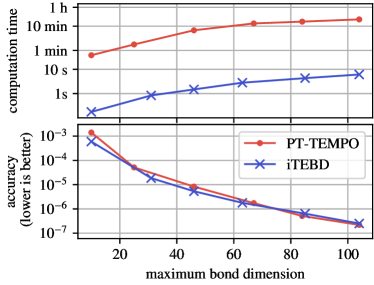
We can further analyse the computational advantage of our algorithm over existing proposals. In particular, we can show that the large computational speedup that we observe is not only due to the reduced number of matrix operations, but also due to an optimal network contraction ‘path’. This is an important issue for contracting two-dimensional tensor networks. For instance, while the original PT-TEMPO algorithm (Ref. [27]) requires $\mathcal{O}(N^{2})$ SVD operations, the divide-and-conquer algorithm presented in Ref. [42] may not lead to significant speedups even though only $\mathcal{O}(N\log{N})$ SVD operations are required. One reason for this is that the bond dimensions that occur during the divide-and-conquer algorithm are generally larger for the same accuracy threshold, as discussed in Ref. [42].

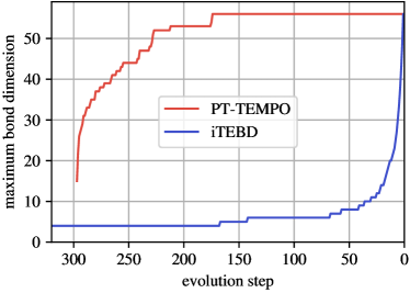
Our proposed algorithm uses an ’anti-diagonal’ contraction from $k=N_{c}$ to $k=0$. Since the bath correlation function decays for large times, the tensors $b(k)$ are only weakly entangling at large $k$. Hence, the bond dimension is expected to remain small at the beginning of the MPS evolution algorithm. To illustrate this, we display in Fig. S4 the bond dimension during the contraction for the two-spin boson model example from the main text (Fig. S3). The bond dimension increases very slowly and reaches the final value only at the last evolution step (slow entanglement growth). In contrast, with PT-TEMPO the bond dimension increases fast. The reason for this is that the PT-TEMPO algorithm contracts rows consisting of tensors with all $k$ values in every step. In the example computation, the maximum bond dimension is reached about half-way through the MPS evolution. Thus, SVDs of tensors with this maximum dimension have to be performed for a large number of contraction steps. In contrast, this most costly SVD is performed only once in the iTEBD scheme.

Finally, we note that for the iTEBD algorithm to produce the best results, $N_{c}$ has to be set large enough for the given SVD truncation threshold. For algebraically decaying bath correlation functions the required $N_{c}$ value can be controlled by introducing a slow exponential cutoff for large times, which typically does not lower the accuracy of the final MPS representation. In fact, the system dynamics up to time $t_{f}$ is not influenced by the behavior of the bath correlation function for $t>t_{f}$. Thus, a cutoff after $t_{f}$ has no effect on the dynamics. Overall, this issue is not severe because the bond dimensions at the beginning of the contraction are very small.

Figure S4: Maximum bond dimension during the network contraction for PT-TEMPO (red) and for the new method based on iTEBD (blue). The system and the parameters are chosen as in Fig. S3. Both algorithms generate a MPS representation of the influence functional with maximum bond dimension 56 (final evolution step ‘0’). For the PT-TEMPO simulation we used the code from Ref. [40] with a relative error SVD truncation threshold of $10^{-7}$. In order to reach the same bond dimension with the iTEBD algorithm we used the threshold $2.8\times 10^{-7}$ (code from Ref. [44]). To ensure a fair comparison, we included an exponential cutoff to the bath correlation function for $t>N\Delta$.

.5 E. Phase transition in the sub-ohmic spin-boson model

We provide further details on the analysis of the phase transition in the sub-ohmic spin-boson model. For weak coupling this model has a unique steady state that obeys the present $Z_{2}$ symmetry [51, 53, 23, 52]. However, the so-called Shiba relation predicts an algebraic decay of $\langle\sigma_{z}\rangle(t)$ due to the algebraic decay of the bath correlation function [23]. Hence, the exact spectrum cannot be gapped because this would imply exponential decay. Thus, a rigorous characterization of the phase transition is more involved. For the $\sigma_{z}$ expectation value we can introduce a continuum approximation of the spectral decomposition (S13)

$$\langle\sigma_{z}\rangle(t)=\sum_{k=1}^{\chi d^{2}}\mathrm{e}^{\gamma_{k}t}\langle\sigma_{z}\rangle_{k}\approx\int_{\gamma\leq 0}\mathrm{d}\gamma\mathrm{e}^{\gamma t}J_{\langle\sigma_{z}\rangle}(\gamma)+\langle\sigma_{z}\rangle_{\mathrm{1}}.$$ (S14)

We have replaced the sum over eigenvalues by an integral introducing the $\sigma_{z}$-spectral density $J_{\langle\sigma_{z}\rangle}(\gamma)$ from which we have explicitly excluded the unique stationary state contribution. Note that due to the symmetry of the model $\langle\sigma_{z}\rangle_{\mathrm{1}}=0$. Algebraic decay towards this stationary value can be realized when the spectral density behaves as $\gamma^{y}$ for small $\gamma$ with some exponent $y$. Assuming a smooth $\sigma_{z}$-spectral density implies that $\langle\sigma_{z}\rangle(t)\rightarrow 0$ for large $t$. However, above the phase transition we find a nonzero stationary value if the initial state is nonsymmetric due to spontaneous symmetry breaking. The only way for this to occur is when a second eigenvector contributes significantly to the asymptotic state. This contribution must then be excluded from the continuum approximation

$$\langle\sigma_{z}\rangle(t)\approx\int_{\gamma\leq 0}\mathrm{d}\gamma\mathrm{e}^{\gamma t}\tilde{J}_{\langle\sigma_{z}\rangle}(\gamma)+\mathrm{e}^{\gamma_{2}t}\langle\sigma_{z}\rangle_{2}.$$ (S15)

In the symmetry broken phase we expect both, $\gamma_{2}=0$ and $\langle\sigma_{z}\rangle_{2}\neq 0$. For the numerics we have to include a low frequency regularization to the bath correlation function. We realize this by enforcing an exponential decay after time $t_{r}$

$$\alpha_{r}(t)=\frac{\alpha(t)}{1+\mathrm{e}^{-\delta(t_{r}-t)}}$$ (S16)

($\delta=0.2\Omega$) in order to ensure stability of the algorithm. The true algebraic decay is recovered when $t_{r}\rightarrow\infty$. Thus, we have to extrapolate to this limit in order to recover the true value of $\langle\sigma_{z}\rangle_{2}$ in the model. In Fig. 4 in the main text we show the low-frequency spectrum of the spin boson model above and below the phase transition and for different $t_{r}$. We can easily identify the rate $\gamma_{2}$ and that it vanishes for large $t_{r}$. The phase transition occurs in the eigenvector $\rho_{2}$ which changes nonanalytically from $\langle\sigma_{z}\rangle_{2}=0$ to $\langle\sigma_{z}\rangle_{2}\neq 0$. Close to the second order transition we expect power law scaling with $t_{r}$ (finite size scaling). Hence, we fit our numerical data with

$$\langle\sigma_{z}\rangle_{2}=\frac{a}{t_{r}^{b}}+c.$$ (S17)

The fit parameter $c$ should then become nonzero above the critical coupling. As shown in Fig. S5 we find very good agreement of our data with the fitted functions, confirming the algebraic behavior. From the predicted asymptotic values of $\sigma_{z}$ (fit parameter $c$) in Fig. 4 (main text) we can identify the critical coupling. Note that the obtained asymptotic values may only be valid in the vicinity of the transition where algebraic behavior is guaranteed.

Figure S5: $\sigma_{z}$ expectation value according to the next-to-leading eigenvector $\rho_{2}$ in the spectral decomposition as a function of the regularization time $t_{r}$. The line plots show the fits with the function (S17).

References

- de Vega and Alonso [2017] I. de Vega and D. Alonso, Dynamics of non-Markovian open quantum systems, Rev. Mod. Phys. 89, 015001 (2017).
- Kaer et al. [2010] P. Kaer, T. R. Nielsen, P. Lodahl, A.-P. Jauho, and J. Mørk, Non-Markovian Model of Photon-Assisted Dephasing by Electron-Phonon Interactions in a Coupled Quantum-Dot–Cavity System, Phys. Rev. Lett. 104, 157401 (2010).
- Madsen et al. [2011] K. H. Madsen, S. Ates, T. Lund-Hansen, A. Löffler, S. Reitzenstein, A. Forchel, and P. Lodahl, Observation of Non-Markovian Dynamics of a Single Quantum Dot in a Micropillar Cavity, Phys. Rev. Lett. 106, 233601 (2011).
- Gröblacher et al. [2015] S. Gröblacher, A. Trubarov, N. Prigge, G. D. Cole, M. Aspelmeyer, and J. Eisert, Observation of non-Markovian micromechanical Brownian motion, Nat. Commun. 6, 1 (2015).
- Segal and Agarwalla [2016] D. Segal and B. K. Agarwalla, Vibrational Heat Transport in Molecular Junctions, Annu. Rev. Phys. Chem. 67, 185 (2016).
- Potočnik et al. [2018] A. Potočnik, A. Bargerbos, F. A. Y. N. Schröder, S. A. Khan, M. C. Collodo, S. Gasparinetti, Y. Salathé, C. Creatore, C. Eichler, H. E. Türeci, A. W. Chin, and A. Wallraff, Studying light-harvesting models with superconducting circuits, Nat. Commun. 9, 1 (2018).
- Tanimura [2020] Y. Tanimura, Numerically “exact” approach to open quantum dynamics: The hierarchical equations of motion (HEOM), J. Chem. Phys. 153, 020901 (2020).
- Wang and Thoss [2008] H. Wang and M. Thoss, From coherent motion to localization: dynamics of the spin-boson model at zero temperature, New J. Phys. 10, 115005 (2008).
- Hartmann and Strunz [2017] R. Hartmann and W. T. Strunz, Exact open quantum system dynamics using the hierarchy of pure states (hops), Journal of Chemical Theory and Computation 13, 5834 (2017).
- Strathearn et al. [2018] A. Strathearn, P. Kirton, D. Kilda, J. Keeling, and B. W. Lovett, Efficient non-Markovian quantum dynamics using time-evolving matrix product operators, Nat. Commun. 9, 3322 (2018).
- Werther and Großmann [2020] M. Werther and F. Großmann, Apoptosis of moving nonorthogonal basis functions in many-particle quantum dynamics, Phys. Rev. B 101, 174315 (2020).
- Kundu and Makri [2023] S. Kundu and N. Makri, PathSum: A C++ and Fortran suite of fully quantum mechanical real-time path integral methods for (multi-)system + bath dynamics, J. Chem. Phys. 158, 224801 (2023).
- Imamoglu [1994] A. Imamoglu, Stochastic wave-function approach to non-Markovian systems, Phys. Rev. A 50, 3650 (1994).
- Garraway [1997] B. M. Garraway, Nonperturbative decay of an atomic system in a cavity, Phys. Rev. A 55, 2290 (1997).
- Mascherpa et al. [2020] F. Mascherpa, A. Smirne, A. D. Somoza, P. Fernández-Acebal, S. Donadi, D. Tamascelli, S. F. Huelga, and M. B. Plenio, Optimized auxiliary oscillators for the simulation of general open quantum systems, Phys. Rev. A 101, 052108 (2020).
- Suess et al. [2014] D. Suess, A. Eisfeld, and W. T. Strunz, Hierarchy of Stochastic Pure States for Open Quantum System Dynamics, Phys. Rev. Lett. 113, 150403 (2014).
- Hughes et al. [2009] K. H. Hughes, C. D. Christ, and I. Burghardt, Effective-mode representation of non-Markovian dynamics: A hierarchical approximation of the spectral density. I. Application to single surface dynamics, J. Chem. Phys. 131, 024109 (2009).
- Prior et al. [2010] J. Prior, A. W. Chin, S. F. Huelga, and M. B. Plenio, Efficient Simulation of Strong System-Environment Interactions, Phys. Rev. Lett. 105, 050404 (2010).
- Lambert et al. [2019] N. Lambert, S. Ahmed, M. Cirio, and F. Nori, Modelling the ultra-strongly coupled spin-boson model with unphysical modes, Nat. Commun. 10, 1 (2019).
- Flannigan et al. [2022] S. Flannigan, F. Damanet, and A. J. Daley, Many-Body Quantum State Diffusion for Non-Markovian Dynamics in Strongly Interacting Systems, Phys. Rev. Lett. 128, 063601 (2022).
- Tang et al. [2015] Z. Tang, X. Ouyang, Z. Gong, H. Wang, and J. Wu, Extended hierarchy equation of motion for the spin-boson model, J. Chem. Phys. 143, 224112 (2015).
- Hartmann et al. [2019] R. Hartmann, M. Werther, F. Grossmann, and W. T. Strunz, Exact open quantum system dynamics: Optimal frequency vs time representation of bath correlations, J. Chem. Phys. 150, 234105 (2019).
- Xu et al. [2022] M. Xu, Y. Yan, Q. Shi, J. Ankerhold, and J. T. Stockburger, Taming Quantum Noise for Efficient Low Temperature Simulations of Open Quantum Systems, Phys. Rev. Lett. 129, 230601 (2022).
- Feynman and Vernon [1963a] R. P. Feynman and F. L. Vernon, The theory of a general quantum system interacting with a linear dissipative system, Ann. Phys. 24, 118 (1963a).
- Pollock et al. [2018] F. A. Pollock, C. Rodríguez-Rosario, T. Frauenheim, M. Paternostro, and K. Modi, Non-Markovian quantum processes: Complete framework and efficient characterization, Phys. Rev. A 97, 012127 (2018).
- Makarov and Makri [1994] D. E. Makarov and N. Makri, Path integrals for dissipative systems by tensor multiplication. Condensed phase quantum dynamics for arbitrarily long time, Chem. Phys. Lett. 221, 482 (1994).
- Jørgensen and Pollock [2019] M. R. Jørgensen and F. A. Pollock, Exploiting the Causal Tensor Network Structure of Quantum Processes to Efficiently Simulate Non-Markovian Path Integrals, Phys. Rev. Lett. 123, 240602 (2019).
- Otterpohl et al. [2022] F. Otterpohl, P. Nalbach, and M. Thorwart, Hidden Phase of the Spin-Boson Model, Phys. Rev. Lett. 129, 120406 (2022).
- Fux et al. [2021] G. E. Fux, E. P. Butler, P. R. Eastham, B. W. Lovett, and J. Keeling, Efficient Exploration of Hamiltonian Parameter Space for Optimal Control of Non-Markovian Open Quantum Systems, Phys. Rev. Lett. 126, 200401 (2021).
- Fux et al. [2023] G. E. Fux, D. Kilda, B. W. Lovett, and J. Keeling, Tensor network simulation of chains of non-Markovian open quantum systems, Phys. Rev. Res. 5, 033078 (2023).
- Fowler-Wright et al. [2022] P. Fowler-Wright, B. W. Lovett, and J. Keeling, Efficient Many-Body Non-Markovian Dynamics of Organic Polaritons, Phys. Rev. Lett. 129, 173001 (2022).
- Gribben et al. [2022] D. Gribben, D. M. Rouse, J. Iles-Smith, A. Strathearn, H. Maguire, P. Kirton, A. Nazir, E. M. Gauger, and B. W. Lovett, Exact dynamics of nonadditive environments in non-markovian open quantum systems, PRX Quantum 3, 010321 (2022).
- Vidal [2007] G. Vidal, Classical Simulation of Infinite-Size Quantum Lattice Systems in One Spatial Dimension, Phys. Rev. Lett. 98, 070201 (2007).
- Note [1] We assume without loss of generality that .
- Link et al. [2022] V. Link, W. T. Strunz, and K. Luoma, Non-Markovian Quantum Dynamics in a Squeezed Reservoir, Entropy 24, 352 (2022).
- Hatano and Suzuki [2005] N. Hatano and M. Suzuki, Finding Exponential Product Formulas of Higher Orders, in Quantum Annealing and Other Optimization Methods (Springer, Berlin, Germany, 2005) pp. 37–68.
- Note [2] Second-order Trotter splitting can be used here (see supplementary material).
- Feynman and Vernon [1963b] R. P. Feynman and F. L. Vernon, The theory of a general quantum system interacting with a linear dissipative system, Ann. Phys. 24, 118 (1963b).
- [39] The supplementary material is appended to this document.
- tem [2023] The TEMPO collaboration, OQuPy (2023).
- Note [3] This is no restriction because the system evolution for time steps only depends on for . Thus, if the correlation function does not decay, we can add an artificial smooth cutoff to the bath correlation for times after .
- Cygorek et al. [2023] M. Cygorek, J. Keeling, B. W. Lovett, and E. M. Gauger, Sublinear scaling in non-Markovian open quantum systems simulations, arXiv 10.48550/arXiv.2304.05291 (2023), 2304.05291 .
- Orús and Vidal [2008] R. Orús and G. Vidal, Infinite time-evolving block decimation algorithm beyond unitary evolution, Phys. Rev. B 78, 155117 (2008).
- [44] A Python implementation of the iTEBD based method is available at github.com/val-link/iTEBD-TEMPO.
- Hartmann and Strunz [2020a] R. Hartmann and W. T. Strunz, Environmentally Induced Entanglement – Anomalous Behavior in the Adiabatic Regime, Quantum 4, 347 (2020a), 2006.04412v2 .
- Minganti et al. [2018] F. Minganti, A. Biella, N. Bartolo, and C. Ciuti, Spectral theory of Liouvillians for dissipative phase transitions, Phys. Rev. A 98, 042118 (2018).
- Debecker et al. [2023] B. Debecker, J. Martin, and F. Damanet, Spectral Theory of Non-Markovian Dissipative Phase Transitions, arXiv 10.48550/arXiv.2307.01119 (2023), 2307.01119 .
- Hartmann and Strunz [2020b] R. Hartmann and W. T. Strunz, Accuracy assessment of perturbative master equations: Embracing nonpositivity, Phys. Rev. A 101, 012103 (2020b).
- Fleming and Cummings [2011] C. H. Fleming and N. I. Cummings, Accuracy of perturbative master equations, Phys. Rev. E 83, 031117 (2011).
- Palacino and Keeling [2021] R. Palacino and J. Keeling, Atom-only theories for U(1) symmetric cavity-QED models, Phys. Rev. Res. 3, L032016 (2021).
- Vojta et al. [2005] M. Vojta, N.-H. Tong, and R. Bulla, Quantum Phase Transitions in the Sub-Ohmic Spin-Boson Model: Failure of the Quantum-Classical Mapping, Phys. Rev. Lett. 94, 070604 (2005).
- Wang and Thoss [2010] H. Wang and M. Thoss, From coherent motion to localization: II. Dynamics of the spin-boson model with sub-Ohmic spectral density at zero temperature, Chem. Phys. 370, 78 (2010).
- Ren et al. [2022] J. Ren, W. Li, T. Jiang, Y. Wang, and Z. Shuai, Time-dependent density matrix renormalization group method for quantum dynamics in complex systems, WIREs Comput. Mol. Sci. 12, e1614 (2022).
- Wang and Shao [2019] H. Wang and J. Shao, Quantum Phase Transition in the Spin-Boson Model: A Multilayer Multiconfiguration Time-Dependent Hartree Study, J. Phys. Chem. A 123, 1882 (2019).
- Note [4] If only tensors are required. In general, open system evolution can always be extended periodically if the dynamical map is known on the full bath memory time [59].
- Zauner-Stauber et al. [2018] V. Zauner-Stauber, L. Vanderstraeten, M. T. Fishman, F. Verstraete, and J. Haegeman, Variational optimization algorithms for uniform matrix product states, Phys. Rev. B 97, 045145 (2018).
- Vanderstraeten et al. [2019] L. Vanderstraeten, J. Haegeman, and F. Verstraete, Tangent-space methods for uniform matrix product states, SciPost Phys. Lect. Notes , 7 (2019).
- Vanhecke et al. [2021] B. Vanhecke, M. V. Damme, J. Haegeman, L. Vanderstraeten, and F. Verstraete, Tangent-space methods for truncating uniform MPS, SciPost Phys. Core 4, 004 (2021).
- Cerrillo and Cao [2014] J. Cerrillo and J. Cao, Non-Markovian Dynamical Maps: Numerical Processing of Open Quantum Trajectories, Phys. Rev. Lett. 112, 110401 (2014).
- Gao et al. [2022] X. Gao, J. Ren, A. Eisfeld, and Z. Shuai, Non-Markovian stochastic Schrödinger equation: Matrix-product-state approach to the hierarchy of pure states, Phys. Rev. A 105, L030202 (2022).