1]\orgdivDepartment of Physics and Astronomy, \orgnameKU Leuven2]\orgdivDepartment of Mathematics, \orgnameKU Leuven

Phase diagram and specific heat of a nonequilibrium Curie–Weiss model

\fnmAaron \surBeyen 0000-0002-4341-7661    \fnmChristian \surMaes 0000-0002-0188-697X    \fnmIrene \surMaes 0000-0001-5734-956X [ [
Abstract

Adding activity or driving to a thermal system may modify its phase diagram and response functions. We study that effect for a Curie-Weiss model where the thermal bath switches rapidly between two temperatures. The critical temperature moves with the nonequilibrium driving, opening up a new region of stability for the paramagnetic phase (zero magnetization) at low temperatures. Furthermore, phase coexistence between the paramagnetic and ferromagnetic phases becomes possible at low temperatures.
Following the excess heat formalism, we calculate the nonequilibrium thermal response and study its behaviour near phase transitions. Where the specific heat at the critical point makes a finite jump in equilibrium (discontinuity), it diverges once we add the second thermal bath. Finally, (also) the nonequilibrium specific heat goes to zero exponentially fast with vanishing temperature, realizing an extended Third Law.

keywords:
Nonequilibrium; Curie-Weiss model; Heat Capacity; Phase diagram

1 Introduction

Little is understood concerning the changes in the phase diagram for a macroscopic system subject to nonequilibrium driving. Even less is known about corresponding modifications in critical behaviour and about their thermal markers, [1]. That includes computing the critical exponent for a possible divergence of heat capacities at the (new) critical points, [2]. The present paper studies those questions for a nonequilibrium mean-field Ising model in the form of a two-temperature Curie-Weiss model, [3]. Multiple-temperature models have been the subject of nonequilibrium modelling for a long time. After all, it often makes physical sense to separate the total system into different subsystems (photons and electrons, or, electronic and lattice degrees of freedom) at different temperatures, [4, 5, 6]. That has been an interesting ingredient for the study of relaxation and transport, and it has also been a subject in the context of steady-state thermodynamics and hydrodynamics, [7]. Two-temperature Ising models have been investigated in various guises as well, [8, 9, 10, 11, 12, 13, 14].
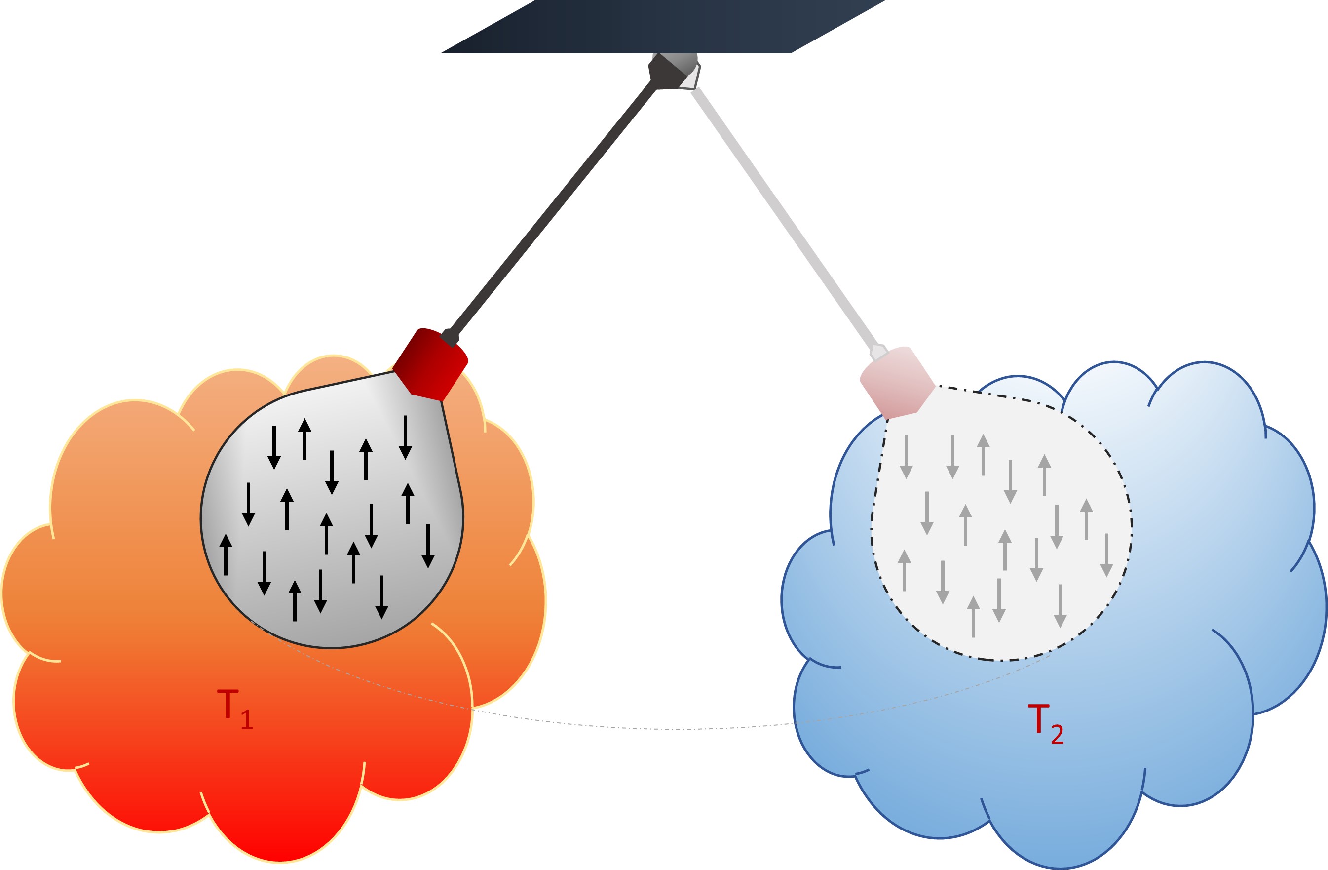
For understanding new many-body physics, here nonequilibrium calorimetry, it is not unusual to start with a mean-field treatment. Yet, for steady spatially extended multiple-temperature spin systems, it is natural to drive the system from installing contacts with different thermal baths at the spatial boundaries. That is not an option for mean-field approaches and we therefore choose a temporal driving. More precisely, we take the system to alternate between two thermal baths, with inverse temperatures β1subscript𝛽1\beta_{1} and β2subscript𝛽2\beta_{2}. The spin dynamics then follow the rules of a Markov jump process (kinetic Ising model [15]) where the heat bath switches between the two temperatures at random times with rate r𝑟r; see Fig. 1. For mathematical simplicity, we consider the limit r𝑟r\uparrow\infty so that the spin-flip rate becomes the sum of the two transition rates, separately satisfying detailed balance with respect to inverse temperature β1subscript𝛽1\beta_{1}, respectively β2subscript𝛽2\beta_{2}, with corresponding heat fluxes.

Refer to caption
Figure 1: Spins in alternating contact with two reservoirs at different temperatures. There is no “average” temperature effectively describing a detailed balance dynamics of the magnetization. Courtesy of Faezeh Khodabandehlou.

The main topics of the present paper are on the one hand the exploration of the nonequilibrium phase diagram, and on the other hand, the computation of nonequilibrium thermal responses in the form of heat capacities. All that is made specific for a two-temperature Curie-Weiss model.
Here is a summary of the findings. First and foremost, the phase diagram as labelled by the stationary magnetization changes compared to equilibrium. New regions of stability open up for macroscopic behaviour that is unstable under equilibrium. For example, even at low temperatures, zero magnetization is still stable, indicating the paramagnetic phase in coexistence with a ferromagnetic phase. Furthermore, the critical values for the temperature and for the quartic spin coupling move with the degree of nonequilibrium.
Secondly, the nonequilibrium specific heat is calculated in the thermodynamic limit. We use the excess heat method applied to the macroscopic dynamics. We study its behaviour through the obtained phase diagram. The specific heat diverges at the phase transitions with critical exponent α=1𝛼1\alpha=1. That starkly contrasts with the equilibrium case, where the specific heat only makes a finite jump [3]. Finally, we check that the computed nonequilibrium specific heat decreases exponentially to zero at low temperatures, realizing a Third Law, [16].

The plan of the paper is as follows. In Sections 2 and 3, we start with a detailed explanation of the model at finite N𝑁N and we derive the macroscopic dynamics (N𝑁N\uparrow\infty), respectively. Next, Section 4 describes the possible phases and phase transitions of the (nonequilibrium) system for zero magnetic field. We present the nonequilibrium specific heats and we discuss their properties in Section 5. The detailed derivation of the specific heat formula is given in Section 6.

2 Finite model

To start, the two-temperature Curie–Weiss model is described for a finite set of spins, and we explain how to calculate the nonequilibrium heat capacity.

2.1 Setup

We have a numbered collection of spins σ=(σ1,σ2,,σN)𝜎subscript𝜎1subscript𝜎2subscript𝜎𝑁\sigma=(\sigma_{1},\sigma_{2},...,\sigma_{N}) for (eventually) large N𝑁N with σi=±1subscript𝜎𝑖plus-or-minus1\sigma_{i}=\pm 1. In the Curie-Weiss format of the Ising model [3], the total energy of the spins equals

E(σ):=JNψ(mN(σ)) with ψ(m):=12m2+hm+g4m4formulae-sequenceassign𝐸𝜎𝐽𝑁𝜓superscript𝑚𝑁𝜎assign with 𝜓𝑚12superscript𝑚2𝑚𝑔4superscript𝑚4E(\sigma):=-JN\psi(m^{N}(\sigma))\qquad\text{ with }\,\psi(m):=\frac{1}{2}m^{2}+hm+\frac{g}{4}m^{4} (1)

only depending on the magnetization

mN(σ):=1Ni=1Nσiassignsuperscript𝑚𝑁𝜎1𝑁superscriptsubscript𝑖1𝑁subscript𝜎𝑖m^{N}(\sigma):=\frac{1}{N}\sum_{i=1}^{N}\sigma_{i}

The parameters J>0𝐽0J>0 (ferromagnetic coupling coefficient), hh (magnetic field), and g>0𝑔0g>0 (quartic interaction) are to be considered as effectively similar to their counterparts in short-range Ising-type models on highly connected (high-dimensional) graphs; see [3, 17].
We are mostly interested in the symmetric case h=00h=0. The quartic term with coupling g𝑔g has been used for modelling quartic interactions, [18, 19, 20] and also appears in the Landau theory of phase transitions [21, 22]. We include it here mainly for completeness and to allow for more complex phase diagrams (even in equilibrium). For example, when g0𝑔0g\neq 0, a coexistence appears between ferro- and paramagnetic phases. Going nonequilibrium also modifies the critical exponent when the specific heat diverges for some g𝑔g.

The dynamics follows a kinetic Ising model [15, 23], where for the total rate, we take a sum of two spin flip rates, each corresponding to a thermal bath. The spin-flip rates separately satisfy local detailed balance (see [24]) with respect to its thermal reservoir, one at inverse temperature β10subscript𝛽10\beta_{1}\geq 0 and the other at β20subscript𝛽20\beta_{2}\geq 0. For definiteness, we take β2β1subscript𝛽2subscript𝛽1\beta_{2}\geq\beta_{1}, i.e., the second bath is at a lower temperature.
The only allowed transitions are between σ=(σ1,σ2,,σk,,σN)𝜎subscript𝜎1subscript𝜎2subscript𝜎𝑘subscript𝜎𝑁\sigma=(\sigma_{1},\sigma_{2},...,\sigma_{k},...,\sigma_{N}) and σk=(σ1,σ2,,σk,,σN)superscript𝜎𝑘subscript𝜎1subscript𝜎2subscript𝜎𝑘subscript𝜎𝑁\sigma^{k}=(\sigma_{1},\sigma_{2},...,-\sigma_{k},...,\sigma_{N}), for some k{1,2,,N}𝑘12𝑁k\in\{1,2,...,N\}, i.e., one spin flip at a time. The (finite) two-temperature Curie-Weiss dynamics is then the Markov process on KN:={1,+1}Nassignsubscript𝐾𝑁superscript11𝑁K_{N}:=\{-1,+1\}^{N} with rates c(σ,k)𝑐𝜎𝑘c(\sigma,k) for flipping from σσk𝜎superscript𝜎𝑘\sigma\to\sigma^{k}:

c(σ,k)𝑐𝜎𝑘\displaystyle c(\sigma,k) =\displaystyle= c1(σ,k)+c2(σ,k),subscript𝑐1𝜎𝑘subscript𝑐2𝜎𝑘\displaystyle c_{1}(\sigma,k)+c_{2}(\sigma,k), (2)
ca(σ,k)subscript𝑐𝑎𝜎𝑘\displaystyle c_{a}(\sigma,k) =\displaystyle= ν(Jβa)neβa2(E(σ)E(σk)),a=1,2formulae-sequence𝜈superscript𝐽subscript𝛽𝑎𝑛superscript𝑒subscript𝛽𝑎2𝐸𝜎𝐸superscript𝜎𝑘𝑎12\displaystyle\frac{\nu}{(J\beta_{a})^{n}}\,e^{\frac{\beta_{a}}{2}(E(\sigma)-E(\sigma^{k}))},\qquad a=1,2 (3)

The reference frequency ν>0𝜈0\nu>0 is added to keep the correct units in (3). It sets the time scale but we are interested only in the asymptotic behaviour t𝑡t\uparrow\infty (after taking the thermodynamic limit), which can not be influenced by ν𝜈\nu. More importantly, a temperature-dependent activation is added in the prefactor of (3), where we recognize an Arrhenius (for n=0𝑛0n=0) or Eyring (for n=1𝑛1n=1) power-law, [25, 26]. In chemical kinetics, these prefactors are usually interpreted as the collision frequency of the molecules in question, increasing with temperature. For spins, there is a similar idea where higher energy/temperature induces more activity (n0𝑛0n\geq 0). In thermal equilibrium with β1=β2subscript𝛽1subscript𝛽2\beta_{1}=\beta_{2}, such prefactors are not important but they can influence the dynamics when out of equilibrium. Kinetic differences (here, for example, already for different n𝑛n) do matter for nonequilibrium phase diagrams and responses. In this paper, to be specific, we compare the case with (n=1)n=1) and without (n=0)𝑛0(n=0) temperature–dependence in the prefactor. Obviously, more general transition rates exist for (3), but we stick to the current choice.

The dynamics (2)–(3) can be seen as the limit r𝑟r\uparrow\infty of a Curie-Weiss model where the temperature switches randomly at rate r𝑟r between the two values; see Fig. 1. Indeed, the case of finite r𝑟r can be modeled by introducing a dichotomous noise ηt{0,1}subscript𝜂𝑡01\eta_{t}\in\{0,1\}, which switches between 00 and 111 at rate r𝑟r [27]. Then,

c~(σ,k)=ηtc1(σ,k)+(1ηt)c2(σ,k)~𝑐𝜎𝑘subscript𝜂𝑡subscript𝑐1𝜎𝑘1subscript𝜂𝑡subscript𝑐2𝜎𝑘\tilde{c}(\sigma,k)=\eta_{t}\ c_{1}(\sigma,k)+(1-\eta_{t})\ c_{2}(\sigma,k) (4)

and the Markov process (ηt,σt)subscript𝜂𝑡subscript𝜎𝑡(\eta_{t},\sigma_{t}) gets correlated. However, in the limit r𝑟r\uparrow\infty, they decorrelate, ηt=12delimited-⟨⟩subscript𝜂𝑡12\langle\eta_{t}\rangle=\frac{1}{2}, and

c~(σ,k)c1(σ,k)+c2(σ,k)2delimited-⟨⟩~𝑐𝜎𝑘subscript𝑐1𝜎𝑘subscript𝑐2𝜎𝑘2\langle\tilde{c}(\sigma,k)\rangle\to\frac{c_{1}(\sigma,k)+c_{2}(\sigma,k)}{2}

where the factor 1212\frac{1}{2} can be absorbed in the time parameter. That averaging obviously does not apply for the temperatures, due to the nonlinearities in (2)–(3) and the absence of global detailed balance.

2.2 The Markov spin-flip dynamics

The backward generator of the Markov process under consideration is LN=L1,N+L2,Nsuperscript𝐿𝑁subscript𝐿1𝑁subscript𝐿2𝑁L^{N}=L_{1,N}+L_{2,N} where, for σ,σKN𝜎superscript𝜎subscript𝐾𝑁\sigma,\sigma^{\prime}\in K_{N},

La,N(σ,σ)={ca(σ,k)if σ=σk for some k{1,2,,N}kca(σ,σk)if σ=σ0 elsesubscript𝐿𝑎𝑁𝜎superscript𝜎casessubscript𝑐𝑎𝜎𝑘if superscript𝜎superscript𝜎𝑘 for some 𝑘12𝑁subscript𝑘subscript𝑐𝑎𝜎superscript𝜎𝑘if 𝜎superscript𝜎0 elseL_{a,N}(\sigma,\sigma^{\prime})=\left\{\begin{array}[]{ll}c_{a}(\sigma,k)&\mbox{if }\sigma^{\prime}=\sigma^{k}\text{ for some }k\in\{1,2,...,N\}\\ -\sum_{k}c_{a}(\sigma,\sigma^{k})&\mbox{if }\sigma=\sigma^{\prime}\\ 0&\mbox{ else}\end{array}\right. (5)

is the backward generator La,Nsubscript𝐿𝑎𝑁L_{a,N} of the Markov jump process when only coupled to temperature bath a=1,2𝑎12a=1,2. The Master equation is

dρtdt=ρtLN=LNρtdsubscript𝜌𝑡d𝑡subscript𝜌𝑡superscript𝐿𝑁superscript𝐿𝑁subscript𝜌𝑡\frac{\textrm{d}\rho_{t}}{\textrm{d}t}=\rho_{t}L^{N}=L^{N\dagger}\rho_{t} (6)

where LNsuperscript𝐿𝑁L^{N\dagger} (forward generator) is the transpose of LNsuperscript𝐿𝑁L^{N}, and the probability ρtsubscript𝜌𝑡\rho_{t} is a row vector of the N𝑁N spins. As a reminder, to settle the notation,

La,Nf(σ)=i=1Nca(σ,i)[f(σi)f(σ)]subscript𝐿𝑎𝑁𝑓𝜎superscriptsubscript𝑖1𝑁subscript𝑐𝑎𝜎𝑖delimited-[]𝑓superscript𝜎𝑖𝑓𝜎\displaystyle L_{a,N}f(\sigma)=\sum_{i=1}^{N}c_{a}(\sigma,i)[f(\sigma^{i})-f(\sigma)] (7)
ddtf(σt)=LNf(σt)f(σt)|σ0=σ=etLNf(σ)formulae-sequencedd𝑡delimited-⟨⟩𝑓subscript𝜎𝑡delimited-⟨⟩superscript𝐿𝑁𝑓subscript𝜎𝑡inner-product𝑓subscript𝜎𝑡subscript𝜎0𝜎superscript𝑒𝑡superscript𝐿𝑁𝑓𝜎\displaystyle\frac{\textrm{d}}{\textrm{d}t}\langle f(\sigma_{t})\rangle=\langle L^{N}f(\sigma_{t})\rangle\qquad\langle f(\sigma_{t})|\sigma_{0}=\sigma\rangle=e^{tL^{N}}f\,(\sigma) (8)

for all functions f:KN:𝑓subscript𝐾𝑁f:K_{N}\rightarrow{\mathbb{R}}.
Finally, there is a unique stationary distribution ρNssuperscriptsubscript𝜌𝑁𝑠\rho_{N}^{s}, stationary solution of (6), satisfying

ρNsLN=0superscriptsubscript𝜌𝑁𝑠superscript𝐿𝑁0\rho_{N}^{s}L^{N}=0

That allows to introduce the stationary expectation Nssuperscriptsubscriptdelimited-⟨⟩𝑁𝑠\langle\cdot\rangle_{N}^{s} and

fNssubscriptsuperscriptdelimited-⟨⟩𝑓𝑠𝑁\displaystyle\langle f\rangle^{s}_{N} =\displaystyle= σKNf(σ)ρNs(σ),LNgNs=0subscript𝜎subscript𝐾𝑁𝑓𝜎superscriptsubscript𝜌𝑁𝑠𝜎superscriptsubscriptdelimited-⟨⟩superscript𝐿𝑁𝑔𝑁𝑠0\displaystyle\sum_{\sigma\in K_{N}}f(\sigma)\,\rho_{N}^{s}(\sigma),\qquad\langle L^{N}g\rangle_{N}^{s}=0 (9)

for arbitrary functions f,g𝑓𝑔f,g on KNsubscript𝐾𝑁K_{N}. Obviously, ρNssuperscriptsubscript𝜌𝑁𝑠\rho_{N}^{s} depends on the two temperatures.

The thermal interpretation (below) is inspired by the case of finite r𝑟r; see Fig. 1. The heat sent to the a𝑎a-th thermal bath during the flipping of the spin at k𝑘k equals

qa,N(σ,k)=1βalogca(σ,k)ca(σk,k)=E(σ)E(σk),a=1,2formulae-sequencesubscript𝑞𝑎𝑁𝜎𝑘1subscript𝛽𝑎subscript𝑐𝑎𝜎𝑘subscript𝑐𝑎superscript𝜎𝑘𝑘𝐸𝜎𝐸superscript𝜎𝑘𝑎12q_{a,N}(\sigma,k)=\frac{1}{\beta_{a}}\log\frac{c_{a}(\sigma,k)}{c_{a}(\sigma^{k},k)}=E(\sigma)-E(\sigma^{k}),\quad a=1,2 (10)

When the configuration is σ𝜎\sigma, the instantaneously expected heat flux (or power) Pa,N(σ)subscript𝑃𝑎𝑁𝜎P_{a,N}(\sigma) to the heat bath a𝑎a is, therefore,

Pa,N(σ)=kca(σ,k)qa,N(σ,k)=La,NE(σ)subscript𝑃𝑎𝑁𝜎subscript𝑘subscript𝑐𝑎𝜎𝑘subscript𝑞𝑎𝑁𝜎𝑘subscript𝐿𝑎𝑁𝐸𝜎P_{a,N}(\sigma)=\sum_{k}c_{a}(\sigma,k)\,q_{a,N}(\sigma,k)=-L_{a,N}E(\sigma) (11)

In the last line, we used the definition (5) of the backward generator La,Nsubscript𝐿𝑎𝑁L_{a,N}. Finally, from (11), the stationary heat flux ja,Nssuperscriptsubscript𝑗𝑎𝑁𝑠j_{a,N}^{s} to the a𝑎a-th reservoir, per number of spins, becomes

ja,Ns=1NPa,NNs=1NLa,NENs=1NLb,NENs=jb,Ns,abformulae-sequencesuperscriptsubscript𝑗𝑎𝑁𝑠1𝑁superscriptsubscriptdelimited-⟨⟩subscript𝑃𝑎𝑁𝑁𝑠1𝑁superscriptsubscriptdelimited-⟨⟩subscript𝐿𝑎𝑁𝐸𝑁𝑠1𝑁superscriptsubscriptdelimited-⟨⟩subscript𝐿𝑏𝑁𝐸𝑁𝑠superscriptsubscript𝑗𝑏𝑁𝑠𝑎𝑏j_{a,N}^{s}=\frac{1}{N}\langle P_{a,N}\rangle_{N}^{s}=-\frac{1}{N}\langle L_{a,N}E\rangle_{N}^{s}=\frac{1}{N}\langle L_{b,N}E\rangle_{N}^{s}=-j_{b,N}^{s},\quad a\neq b (12)

where we used La,NENs=Lb,NENssuperscriptsubscriptdelimited-⟨⟩subscript𝐿𝑎𝑁𝐸𝑁𝑠superscriptsubscriptdelimited-⟨⟩subscript𝐿𝑏𝑁𝐸𝑁𝑠\langle L_{a,N}E\rangle_{N}^{s}=-\langle L_{b,N}E\rangle_{N}^{s} when ab𝑎𝑏a\neq b (see (9)) and where the energy function E𝐸E needs to be taken from (1).

2.3 Excess heat, quasipotential and heat capacity

The definition of nonequilibrium heat capacity follows the excess heat framework discussed in [16, 28, 29]. To be more self-contained, we use Fig. 2 to guide the reader.

Qab(N),exsubscriptsuperscript𝑄𝑁ex𝑎𝑏Q^{(N),\text{ex}}_{ab}

Cab,neq(N)=δQab(N),exdTbsubscriptsuperscript𝐶𝑁𝑎𝑏neq𝛿subscriptsuperscript𝑄𝑁ex𝑎𝑏dsubscript𝑇𝑏C^{(N)}_{ab,\text{neq}}=\frac{\delta Q^{(N),\text{ex}}_{ab}}{\textrm{d}T_{b}}

Tb,0subscript𝑇𝑏0T_{b,0}

Tb,fsubscript𝑇𝑏𝑓T_{b,f}

Qab,f(N),hksuperscriptsubscript𝑄𝑎𝑏𝑓𝑁hkQ_{ab,f}^{(N),\text{hk}}

//

0

Nja,Ns𝑁superscriptsubscript𝑗𝑎𝑁𝑠Nj_{a,N}^{s}

Time t𝑡tPower Pa,Nsubscript𝑃𝑎𝑁P_{a,N}
Figure 2: Cartoon of the heat flux or power Pa,Nsubscript𝑃𝑎𝑁P_{a,N} as a function of time for a relaxation process when changing the temperature Tb,0Tb,f=Tb,0+dTbsubscript𝑇𝑏0subscript𝑇𝑏𝑓subscript𝑇𝑏0dsubscript𝑇𝑏T_{b,0}\rightarrow T_{b,f}=T_{b,0}+\textrm{d}T_{b}. There are two sources of heat (time-integrated power): the excess heat Qab(N),exsubscriptsuperscript𝑄𝑁ex𝑎𝑏Q^{(N),\text{ex}}_{ab} and the housekeeping heat Qab(N),hksubscriptsuperscript𝑄𝑁hk𝑎𝑏Q^{(N),\text{hk}}_{ab}. In the quasistatic limit, the nonequilibrium heat capacity is given by Cab,neq(N)=δQab(N),exdTbsubscriptsuperscript𝐶𝑁𝑎𝑏neq𝛿subscriptsuperscript𝑄𝑁ex𝑎𝑏dsubscript𝑇𝑏C^{(N)}_{ab,\text{neq}}=\frac{\delta Q^{(N),\text{ex}}_{ab}}{\textrm{d}T_{b}}; see (15) for more precision. (Made in Tikz).

One imagines that the system is in a steady nonequilibrium condition before time t=0𝑡0t=0. The temperature of the two heat baths is fixed, Tb,0subscript𝑇𝑏0T_{b,0} being the temperature of bath b𝑏b. Obviously, the spin configuration σ0=σsubscript𝜎0𝜎\sigma_{0}=\sigma at time t=0𝑡0t=0 is random, and follows distribution ρNssubscriptsuperscript𝜌𝑠𝑁\rho^{s}_{N} at Tb,0subscript𝑇𝑏0T_{b,0}. At time t=0𝑡0t=0 we slightly change the temperature Tb,0Tb,f=Tb,0+dTbsubscript𝑇𝑏0subscript𝑇𝑏𝑓subscript𝑇𝑏0dsubscript𝑇𝑏T_{b,0}\longrightarrow T_{b,f}=T_{b,0}+\textrm{d}T_{b}. There will now start a relaxation to a new steady condition; the ρNssubscriptsuperscript𝜌𝑠𝑁\rho^{s}_{N} for Tb,0subscript𝑇𝑏0T_{b,0} will converge to the ρNssubscriptsuperscript𝜌𝑠𝑁\rho^{s}_{N} for Tb,fsubscript𝑇𝑏𝑓T_{b,f}. That takes time of course, while the system is exposed to Tb,fsubscript𝑇𝑏𝑓T_{b,f} in heat bath b𝑏b while the temperature in heat bath a𝑎a has not changed. At times t>0𝑡0t>0, the power dissipated in heat bath a𝑎a is Pa,N(σt)subscript𝑃𝑎𝑁subscript𝜎𝑡P_{a,N}(\sigma_{t}) with Markov process conditional expectation Pa,N(σt)|σ0=σNsubscriptinner-productsubscript𝑃𝑎𝑁subscript𝜎𝑡subscript𝜎0𝜎𝑁\langle P_{a,N}(\sigma_{t})\,|\,\sigma_{0}=\sigma\rangle_{N}. Asymptotically, for t𝑡t\uparrow\infty the expected dissipated power converges to Nja,Ns𝑁superscriptsubscript𝑗𝑎𝑁𝑠Nj_{a,N}^{s} for temperature Tb,fsubscript𝑇𝑏𝑓T_{b,f} in heat bath b𝑏b (see Fig. 2). Therefore, the excess heat to heat bath a𝑎a is estimated by the time integral of the difference,

Va(N)(σ):=0dt[Pa,N(σt)|σ0=σNNja,Ns]assignsubscriptsuperscript𝑉𝑁𝑎𝜎superscriptsubscript0d𝑡delimited-[]subscriptinner-productsubscript𝑃𝑎𝑁subscript𝜎𝑡subscript𝜎0𝜎𝑁𝑁superscriptsubscript𝑗𝑎𝑁𝑠V^{(N)}_{a}(\sigma):=\int_{0}^{\infty}\textrm{d}t\,[\langle P_{a,N}(\sigma_{t})|\sigma_{0}=\sigma\rangle_{N}-Nj_{a,N}^{s}] (13)

Note that the integral is converging since

limtPa,N(σt)|σ0=σN=Nja,Nssubscript𝑡subscriptinner-productsubscript𝑃𝑎𝑁subscript𝜎𝑡subscript𝜎0𝜎𝑁𝑁superscriptsubscript𝑗𝑎𝑁𝑠\lim_{t\uparrow\infty}\langle P_{a,N}(\sigma_{t})\,|\,\sigma_{0}=\sigma\rangle_{N}=Nj_{a,N}^{s}

exponentially fast, uniformly in σ𝜎\sigma, as a standard consequence of the Perron–Frobenius theorem [30]. Similarly,

Va(N)Ns=0subscriptsuperscriptdelimited-⟨⟩subscriptsuperscript𝑉𝑁𝑎𝑠𝑁0\langle V^{(N)}_{a}\rangle^{s}_{N}=0 (14)

and the dynamics in (13) and the stationary distribution are all at temperature Tb,fsubscript𝑇𝑏𝑓T_{b,f}.
The time-integral (13) makes Va(N)(σ)subscriptsuperscript𝑉𝑁𝑎𝜎V^{(N)}_{a}(\sigma) a measure of the excess heat, indicated by Qab(N),exsubscriptsuperscript𝑄𝑁ex𝑎𝑏Q^{(N),\text{ex}}_{ab} in Fig. 2. It is the heat that is in excess with respect to the housekeeping heat Qab(N),hksubscriptsuperscript𝑄𝑁hk𝑎𝑏Q^{(N),\text{hk}}_{ab} also indicated in Fig. 2, and is entirely due to the relaxation from the original steady nonequilibrium condition to the final one. It is indeed important to realize that dissipation is already present even before any parameter, like the temperature, is changed. The nonequilibrium heat capacity Cab(N)subscriptsuperscript𝐶𝑁𝑎𝑏C^{(N)}_{ab} can therefore be defined as the thermal response of Qab(N),exsubscriptsuperscript𝑄𝑁ex𝑎𝑏Q^{(N),\text{ex}}_{ab} to a change in temperature in heat bath b𝑏b.
A more precise analysis takes the previous heuristics through a quasistatic limit (which is the reason we did not immediately identify Qab(N),exsubscriptsuperscript𝑄𝑁ex𝑎𝑏Q^{(N),\text{ex}}_{ab} with Va(N)subscriptsuperscript𝑉𝑁𝑎V^{(N)}_{a}) but the idea is unchanged:
For each finite N𝑁N, the nonequilibrium heat capacity Cab(N)superscriptsubscript𝐶𝑎𝑏𝑁C_{ab}^{(N)} from measuring the excess heat flux from bath a𝑎a due to a change in the temperature of reservoir b𝑏b (a,b=1,2formulae-sequence𝑎𝑏12a,b=1,2) equals

Cab(N)=Va(N)TbNs=kBβb2Va(N)βbNssuperscriptsubscript𝐶𝑎𝑏𝑁superscriptsubscriptdelimited-⟨⟩superscriptsubscript𝑉𝑎𝑁subscript𝑇𝑏𝑁𝑠subscript𝑘𝐵superscriptsubscript𝛽𝑏2superscriptsubscriptdelimited-⟨⟩superscriptsubscript𝑉𝑎𝑁subscript𝛽𝑏𝑁𝑠C_{ab}^{(N)}=-\left\langle\frac{\partial V_{a}^{(N)}}{\partial T_{b}}\right\rangle_{N}^{s}=k_{B}\beta_{b}^{2}\left\langle\frac{\partial V_{a}^{(N)}}{\partial\beta_{b}}\right\rangle_{N}^{s} (15)

The sum

Cb(N)=Cab(N)+Cbb(N),baformulae-sequencesuperscriptsubscript𝐶𝑏𝑁superscriptsubscript𝐶𝑎𝑏𝑁superscriptsubscript𝐶𝑏𝑏𝑁𝑏𝑎C_{b}^{(N)}=C_{ab}^{(N)}+C_{bb}^{(N)},\qquad b\neq a

measures the thermal susceptibility of the total environment (both thermal reservoirs combined) to changes in reservoir temperature Tbsubscript𝑇𝑏T_{b}. Experimentally, a nonequilibrium heat capacity can be obtained from AC-calorimetry measurements, see [31]. For computational purposes, it is interesting to observe that the integral equation (13) can be reduced to the following equivalent Poisson equation for Va(N)subscriptsuperscript𝑉𝑁𝑎V^{(N)}_{a},

LNVa(N)superscript𝐿𝑁subscriptsuperscript𝑉𝑁𝑎\displaystyle L^{N}V^{(N)}_{a} =Nja,NsPa,Nabsent𝑁superscriptsubscript𝑗𝑎𝑁𝑠subscript𝑃𝑎𝑁\displaystyle=Nj_{a,N}^{s}-P_{a,N} (16)
=La,NELa,NENsabsentsubscript𝐿𝑎𝑁𝐸subscriptsuperscriptdelimited-⟨⟩subscript𝐿𝑎𝑁𝐸𝑠𝑁\displaystyle=L_{a,N}E-\langle L_{a,N}E\rangle^{s}_{N}
=La,NE+Lb,NENs,baformulae-sequenceabsentsubscript𝐿𝑎𝑁𝐸subscriptsuperscriptdelimited-⟨⟩subscript𝐿𝑏𝑁𝐸𝑠𝑁𝑏𝑎\displaystyle=L_{a,N}E+\langle L_{b,N}E\rangle^{s}_{N},\qquad b\neq a (17)

where we used that La,NENs=Lb,NENssuperscriptsubscriptdelimited-⟨⟩subscript𝐿𝑎𝑁𝐸𝑁𝑠superscriptsubscriptdelimited-⟨⟩subscript𝐿𝑏𝑁𝐸𝑁𝑠\langle L_{a,N}E\rangle_{N}^{s}=-\langle L_{b,N}E\rangle_{N}^{s} when ab𝑎𝑏a\neq b in the last line; see (9).
We see immediately from (17) that

LN(V1(N)+V2(N))=LNEsuperscript𝐿𝑁superscriptsubscript𝑉1𝑁superscriptsubscript𝑉2𝑁superscript𝐿𝑁𝐸L^{N}(V_{1}^{(N)}+V_{2}^{(N)})=L^{N}E

which implies that the sum always satisfies

V1(N)+V2(N)=EENssuperscriptsubscript𝑉1𝑁superscriptsubscript𝑉2𝑁𝐸subscriptsuperscriptdelimited-⟨⟩𝐸𝑠𝑁V_{1}^{(N)}+V_{2}^{(N)}=E-\langle E\rangle^{s}_{N}

which motivates also to call Va(N)superscriptsubscript𝑉𝑎𝑁V_{a}^{(N)} a quasipotential.

As a simple illustration of the above thermal setup, in Appendix A we give the explicit solution for the case of only N=2𝑁2N=2 spins σ1,σ2subscript𝜎1subscript𝜎2\sigma_{1},\sigma_{2}. Clearly, that system is not macroscopic but it already gives an interesting nonequilibrium generalization (of many independent and identical copies) of the well-known two-level system, showing e.g. negative heat capacities. It also allows the reader to get acquainted with the excess heat formalism briefly introduced above.

3 Macroscopic dynamics

When the number N𝑁N of spins gets very large, simplifications and greater interest arise, which we explain in this section. In particular, we show here that in the thermodynamic limit, the magnetization follows a first-order equation in time.

3.1 Propagation of molecular chaos

Consider the Bernoulli product probability distributions ρmsuperscriptsubscript𝜌𝑚tensor-product\rho_{m}^{\otimes} on {+1,1}>0superscript11subscriptabsent0\{+1,-1\}^{{\mathbb{N}}_{>0}} with parameter m[1,1]𝑚11m\in[-1,1], formally defined as

ρm(σ)=1+mσ2superscriptsubscript𝜌𝑚tensor-product𝜎subscriptproduct1𝑚subscript𝜎2\rho_{m}^{\otimes}(\sigma)=\prod_{\ell}\frac{1+m\sigma_{\ell}}{2}

with corresponding expectation msubscriptdelimited-⟨⟩𝑚\langle\cdot\rangle_{m}; σ1σ2σkm=mksubscriptdelimited-⟨⟩subscript𝜎1subscript𝜎2subscript𝜎𝑘𝑚superscript𝑚𝑘\langle\sigma_{1}\sigma_{2}\ldots\sigma_{k}\rangle_{m}=m^{k}. Note that for that probability distribution, mN(σ)m=msubscriptdelimited-⟨⟩superscript𝑚𝑁𝜎𝑚𝑚\langle m^{N}(\sigma)\rangle_{m}=m, such that by the strong law of large numbers, mN(σ)msuperscript𝑚𝑁𝜎𝑚m^{N}(\sigma)\rightarrow m with probability one.
In other words, for any continuous function f:[1,1]×{+1,1}k:𝑓11superscript11𝑘f:[-1,1]\times\{+1,-1\}^{k} with k>0𝑘subscriptabsent0k\in{\mathbb{N}}_{>0},

limNf(mN(σ),σ1,,σk)m=f(m,σ1,,σk)msubscript𝑁subscriptdelimited-⟨⟩𝑓superscript𝑚𝑁𝜎subscript𝜎1subscript𝜎𝑘𝑚subscriptdelimited-⟨⟩𝑓𝑚subscript𝜎1subscript𝜎𝑘𝑚\lim_{N}\langle f(m^{N}(\sigma),\sigma_{1},\dots,\sigma_{k})\rangle_{m}=\langle f(m,\sigma_{1},\dots,\sigma_{k})\rangle_{m} (18)

where we still average over the spins σ1,,σksubscript𝜎1subscript𝜎𝑘\sigma_{1},...,\sigma_{k} in the last expression.

Imagine now that at time zero t=0𝑡0t=0, the spins are sampled from ρmsuperscriptsubscript𝜌𝑚tensor-product\rho_{m}^{\otimes} with given magnetization m[1,1]𝑚11m\in[-1,1]. We claim, as is typical for mean-field systems in the limit N𝑁N\uparrow\infty , that the spins at later times t0𝑡0t\geq 0 follow a product distribution ρmtsuperscriptsubscript𝜌subscript𝑚𝑡tensor-product\rho_{m_{t}}^{\otimes} as well provided that

dmtdt=H(mt):=H1(mt)+H2(mt),m0=mformulae-sequencedsubscript𝑚𝑡d𝑡𝐻subscript𝑚𝑡assignsubscript𝐻1subscript𝑚𝑡subscript𝐻2subscript𝑚𝑡subscript𝑚0𝑚\frac{\textrm{d}m_{t}}{\textrm{d}t}=H(m_{t}):=H_{1}(m_{t})+H_{2}(m_{t}),\quad m_{0}=m (19)

for

Ha(m):=2ν(Jβa)n(sinhJβaψ(m)mcoshJβaψ(m))assignsubscript𝐻𝑎𝑚2𝜈superscript𝐽subscript𝛽𝑎𝑛𝐽subscript𝛽𝑎superscript𝜓𝑚𝑚𝐽subscript𝛽𝑎superscript𝜓𝑚H_{a}(m):=\frac{2\nu}{(J\beta_{a})^{n}}\Big{(}\sinh{J\beta_{a}\psi^{\prime}(m)}-m\,\cosh{J\beta_{a}\psi^{\prime}(m)}\Big{)} (20)

We call that claim the propagation of chaos, [32, 33], indicating that the spins remain statistically independent in the limit N𝑁N\uparrow\infty,
To show that propagation of chaos, we will prove that the weak limit of the forward generator La,Nsuperscriptsubscript𝐿𝑎𝑁L_{a,N}^{\dagger} (transpose of La,Nsubscript𝐿𝑎𝑁L_{a,N}) satisfies

L+ρm:=limNa=12La,N+ρm=H(m)ρmmassignsuperscript𝐿superscriptsubscript𝜌𝑚tensor-productsubscript𝑁superscriptsubscript𝑎12subscriptsuperscript𝐿𝑎𝑁superscriptsubscript𝜌𝑚tensor-product𝐻𝑚superscriptsubscript𝜌𝑚tensor-product𝑚L^{+}\rho_{m}^{\otimes}:=\lim_{N}\sum_{a=1}^{2}L^{+}_{a,N}\rho_{m}^{\otimes}=H(m)\,\frac{\partial\rho_{m}^{\otimes}}{\partial m} (21)

As a consequence of (21), if indeed (mt,t0)subscript𝑚𝑡𝑡0(m_{t},t\geq 0) is a solution of (19), then

ddtρmt=ρmtmtdmtdt=ρmtmtH(mt)=Lρmtdd𝑡superscriptsubscript𝜌subscript𝑚𝑡tensor-productsuperscriptsubscript𝜌subscript𝑚𝑡tensor-productsubscript𝑚𝑡dsubscript𝑚𝑡d𝑡superscriptsubscript𝜌subscript𝑚𝑡tensor-productsubscript𝑚𝑡𝐻subscript𝑚𝑡superscript𝐿superscriptsubscript𝜌subscript𝑚𝑡tensor-product\frac{\textrm{d}}{\textrm{d}t}\rho_{m_{t}}^{\otimes}=\frac{\partial\rho_{m_{t}}^{\otimes}}{\partial m_{t}}\frac{\textrm{d}m_{t}}{\textrm{d}t}=\frac{\partial\rho_{m_{t}}^{\otimes}}{\partial m_{t}}H(m_{t})=L^{\dagger}\rho_{m_{t}}^{\otimes}

and hence ρmtsuperscriptsubscript𝜌subscript𝑚𝑡tensor-product\rho_{m_{t}}^{\otimes} is the solution of the (infinite volume) Master equation (6) (which is the property of propagation of chaos). Since the solution to the Master equation is unique, it follows that, in the limit N𝑁N\uparrow\infty, we are only interested in a dynamics satisfying (19).

Proof of (21).

The forward generator La,Nsuperscriptsubscript𝐿𝑎𝑁L_{a,N}^{\dagger} acts as

σg(σ)La,Nρm(σ)subscript𝜎𝑔𝜎superscriptsubscript𝐿𝑎𝑁superscriptsubscript𝜌𝑚tensor-product𝜎\displaystyle\sum_{\sigma}g(\sigma)\,L_{a,N}^{\dagger}\rho_{m}^{\otimes}(\sigma) =\displaystyle= σg(σ)i=1k[ca(σi,i)ρm(σi)ca(σ,i)ρm(σ)]subscript𝜎𝑔𝜎superscriptsubscript𝑖1𝑘delimited-[]subscript𝑐𝑎superscript𝜎𝑖𝑖superscriptsubscript𝜌𝑚tensor-productsuperscript𝜎𝑖subscript𝑐𝑎𝜎𝑖superscriptsubscript𝜌𝑚tensor-product𝜎\displaystyle\sum_{\sigma}g(\sigma)\sum_{i=1}^{k}\left[c_{a}(\sigma^{i},i)\rho_{m}^{\otimes}(\sigma^{i})-c_{a}(\sigma,i)\rho_{m}^{\otimes}(\sigma)\right] (22)

for arbitrary g(σ)=g(σ1,,σk),kNformulae-sequence𝑔𝜎𝑔subscript𝜎1subscript𝜎𝑘𝑘𝑁g(\sigma)=g(\sigma_{1},\ldots,\sigma_{k}),k\leq N. We can use here the asymptotics

ca(σ,k)=ν(Jβa)neJβaσkψ(mN(σ)){1+βaJNψ′′(mN(σ))+O(1N2)}subscript𝑐𝑎𝜎𝑘𝜈superscript𝐽subscript𝛽𝑎𝑛superscript𝑒𝐽subscript𝛽𝑎subscript𝜎𝑘superscript𝜓superscript𝑚𝑁𝜎1subscript𝛽𝑎𝐽𝑁superscript𝜓′′superscript𝑚𝑁𝜎𝑂1superscript𝑁2c_{a}(\sigma,k)=\frac{\nu}{(J\beta_{a})^{n}}\,e^{-J\beta_{a}\sigma_{k}\,\psi^{\prime}(m^{N}(\sigma))}\left\{1+\frac{\beta_{a}J}{N}\psi^{\prime\prime}(m^{N}(\sigma))+O\left(\frac{1}{N^{2}}\right)\right\} (23)

Noting further that

ρm(σi)=ρm(σ)1mσi1+mσisuperscriptsubscript𝜌𝑚tensor-productsuperscript𝜎𝑖superscriptsubscript𝜌𝑚tensor-product𝜎1𝑚subscript𝜎𝑖1𝑚subscript𝜎𝑖\rho_{m}^{\otimes}(\sigma^{i})=\rho_{m}^{\otimes}(\sigma)\frac{1-m\sigma_{i}}{1+m\sigma_{i}}

the right-hand side of (22) equals

ν(Jβa)ng(σ)i=1k[1mσi1+mσieJβaσiψ(mN(σ))eJβaσiψ(mN(σ))]m+O(1N)𝜈superscript𝐽subscript𝛽𝑎𝑛subscriptdelimited-⟨⟩𝑔𝜎superscriptsubscript𝑖1𝑘delimited-[]1𝑚subscript𝜎𝑖1𝑚subscript𝜎𝑖superscript𝑒𝐽subscript𝛽𝑎subscript𝜎𝑖superscript𝜓superscript𝑚𝑁𝜎superscript𝑒𝐽subscript𝛽𝑎subscript𝜎𝑖superscript𝜓superscript𝑚𝑁𝜎𝑚𝑂1𝑁\displaystyle\frac{\nu}{(J\beta_{a})^{n}}\left\langle g(\sigma)\sum_{i=1}^{k}\left[\frac{1-m\sigma_{i}}{1+m\sigma_{i}}e^{J\beta_{a}\sigma_{i}\,\psi^{\prime}(m^{N}(\sigma))}-e^{-J\beta_{a}\sigma_{i}\,\psi^{\prime}(m^{N}(\sigma))}\right]\right\rangle_{m}+O\left(\frac{1}{N}\right)

and hence, up to order O(1N)𝑂1𝑁O\left(\frac{1}{N}\right),

σa=12g(σ)La,Nρm(σ)=subscript𝜎superscriptsubscript𝑎12𝑔𝜎superscriptsubscript𝐿𝑎𝑁superscriptsubscript𝜌𝑚tensor-product𝜎absent\displaystyle\sum_{\sigma}\sum_{a=1}^{2}g(\sigma)\,L_{a,N}^{\dagger}\rho_{m}^{\otimes}(\sigma)=
a=12ν(Jβa)ng(σ)i=1k[1mσi1+mσieJβaσiψ(m)eJβaσiψ(m)]msuperscriptsubscript𝑎12𝜈superscript𝐽subscript𝛽𝑎𝑛subscriptdelimited-⟨⟩𝑔𝜎superscriptsubscript𝑖1𝑘delimited-[]1𝑚subscript𝜎𝑖1𝑚subscript𝜎𝑖superscript𝑒𝐽subscript𝛽𝑎subscript𝜎𝑖superscript𝜓𝑚superscript𝑒𝐽subscript𝛽𝑎subscript𝜎𝑖superscript𝜓𝑚𝑚\displaystyle\sum_{a=1}^{2}\frac{\nu}{(J\beta_{a})^{n}}\left\langle g(\sigma)\sum_{i=1}^{k}\left[\frac{1-m\sigma_{i}}{1+m\sigma_{i}}e^{J\beta_{a}\sigma_{i}\,\psi^{\prime}(m)}-e^{-J\beta_{a}\sigma_{i}\,\psi^{\prime}(m)}\right]\right\rangle_{m}
a=12ν(Jβa)ng(σ)i=1k2σi1+mσi[sinhβaJψ(m)mcoshβaJψ(m)]m=superscriptsubscript𝑎12𝜈superscript𝐽subscript𝛽𝑎𝑛subscriptdelimited-⟨⟩𝑔𝜎superscriptsubscript𝑖1𝑘2subscript𝜎𝑖1𝑚subscript𝜎𝑖delimited-[]subscript𝛽𝑎𝐽superscript𝜓𝑚𝑚subscript𝛽𝑎𝐽superscript𝜓𝑚𝑚absent\displaystyle\sum_{a=1}^{2}\frac{\nu}{(J\beta_{a})^{n}}\left\langle g(\sigma)\sum_{i=1}^{k}\frac{2\sigma_{i}}{1+m\sigma_{i}}\left[\sinh{\beta_{a}J\psi^{\prime}(m)}-m\cosh{\beta_{a}J\psi^{\prime}(m)}\right]\right\rangle_{m}=
=σg(σ)a=12Ha(m)ρmm(σ)=σg(σ)H(m)ρmm(σ)absentsubscript𝜎𝑔𝜎superscriptsubscript𝑎12subscript𝐻𝑎𝑚superscriptsubscript𝜌𝑚tensor-product𝑚𝜎subscript𝜎𝑔𝜎𝐻𝑚superscriptsubscript𝜌𝑚tensor-product𝑚𝜎\displaystyle=\sum_{\sigma}g(\sigma)\sum_{a=1}^{2}H_{a}(m)\frac{\partial\rho_{m}^{\otimes}}{\partial m}(\sigma)=\sum_{\sigma}g(\sigma)H(m)\frac{\partial\rho_{m}^{\otimes}}{\partial m}(\sigma) (24)

where we used in the last line the definition (20) of Hasubscript𝐻𝑎H_{a} together with the fact that, formally,

ρmm(σ)=m(i1+mσi2)=ρm(σ)iσi1+mσisuperscriptsubscript𝜌𝑚tensor-product𝑚𝜎𝑚subscriptproduct𝑖1𝑚subscript𝜎𝑖2superscriptsubscript𝜌𝑚tensor-product𝜎subscript𝑖subscript𝜎𝑖1𝑚subscript𝜎𝑖\displaystyle\frac{\partial\rho_{m}^{\otimes}}{\partial m}(\sigma)=\frac{\partial}{\partial m}\Big{(}\prod_{i}\frac{1+m\sigma_{i}}{2}\Big{)}=\rho_{m}^{\otimes}(\sigma)\,\sum_{i}\frac{\sigma_{i}}{1+m\sigma_{i}}

Since (24) holds for arbitrary functions g𝑔g (depending on a finite number of spins), the weak limit (21) is proven. ∎

3.2 Magnetization dynamics

The function H=H1+H2𝐻subscript𝐻1subscript𝐻2H=H_{1}+H_{2}, defined from (20), is smooth in m[1,+1]𝑚11m\in[-1,+1] and satisfies

H(±1)=H1(±1)+H2(±1)=2ν(eJβ1ψ(±1)(Jβ1)n+eJβ2ψ(±1)(Jβ2)n)𝐻plus-or-minus1subscript𝐻1plus-or-minus1subscript𝐻2plus-or-minus1minus-or-plus2𝜈superscript𝑒𝐽subscript𝛽1superscript𝜓plus-or-minus1superscript𝐽subscript𝛽1𝑛superscript𝑒𝐽subscript𝛽2superscript𝜓plus-or-minus1superscript𝐽subscript𝛽2𝑛H(\pm 1)=H_{1}(\pm 1)+H_{2}(\pm 1)=\mp 2\nu\left(\frac{e^{-J\beta_{1}\psi^{\prime}(\pm 1)}}{(J\beta_{1})^{n}}+\frac{e^{-J\beta_{2}\psi^{\prime}(\pm 1)}}{(J\beta_{2})^{n}}\right)

such that sgn(H(±1))=1sgn𝐻plus-or-minus1minus-or-plus1\text{sgn}(H(\pm 1))=\mp 1. As a consequence, by looking at (19), if m0[1,1]subscript𝑚011m_{0}\in[-1,1], then also mt[1,1]subscript𝑚𝑡11m_{t}\in[-1,1] for all t𝑡t, and thus (e.g., from the Picard–Lindelöf theorem [34]), the solution mtsubscript𝑚𝑡m_{t} to the initial value problem exists and is unique for all times t0𝑡0t\geq 0.
In more detail,

dmtdt=H1(mt)+H2(mt)=2ν4nJn(4β2δ2)n[\displaystyle\frac{\textrm{d}m_{t}}{\textrm{d}t}=H_{1}(m_{t})+H_{2}(m_{t})=\frac{2\nu\cdot 4^{n}}{J^{n}(4\beta^{2}-\delta^{2})^{n}}\Biggl{[}
((βδ2)n+(β+δ2)n)cosh(δ2ψ(mt))(sinhβψ(mt)mtcoshβψ(mt))superscript𝛽𝛿2𝑛superscript𝛽𝛿2𝑛𝛿2superscript𝜓subscript𝑚𝑡𝛽superscript𝜓subscript𝑚𝑡subscript𝑚𝑡𝛽superscript𝜓subscript𝑚𝑡\displaystyle\left((\beta-\frac{\delta}{2})^{n}+(\beta+\frac{\delta}{2})^{n}\right)\cosh{(\frac{\delta}{2}\psi^{\prime}(m_{t}))}\Big{(}\sinh{\beta\psi^{\prime}(m_{t})}-m_{t}\cosh{\beta\psi^{\prime}(m_{t})}\Big{)}
+((β+δ2)n(βδ2)n)sinh(δ2ψ(mt))(mtsinhβψ(mt)coshβψ(mt))]\displaystyle+\left((\beta+\frac{\delta}{2})^{n}-(\beta-\frac{\delta}{2})^{n}\right)\sinh{(\frac{\delta}{2}\psi^{\prime}(m_{t}))}\Big{(}m_{t}\sinh{\beta\psi^{\prime}(m_{t})}-\cosh{\beta\psi^{\prime}(m_{t})}\Big{)}\Biggr{]} (25)

Here and in what follows, we use the dimensionless quantities

β=J2(β1+β2)δ=J(β2β1)0formulae-sequence𝛽𝐽2subscript𝛽1subscript𝛽2𝛿𝐽subscript𝛽2subscript𝛽10\beta=\frac{J}{2}(\,\beta_{1}+\beta_{2}\,)\qquad\delta=J(\beta_{2}-\beta_{1})\geq 0 (26)

where the parameter δ𝛿\delta characterizes the degree of nonequilibrium. Even though β,δ𝛽𝛿\beta,\delta are dimensionless, we often refer to them as the mean inverse temperature and inverse temperature difference, respectively. Note that β10subscript𝛽10\beta_{1}\geq 0 implies the constraint βδ2𝛽𝛿2\beta\geq\frac{\delta}{2} but δ𝛿\delta need not be small.

Stationary values msubscript𝑚m_{*} of the magnetization satisfy H1(m)+H2(m)=0subscript𝐻1subscript𝑚subscript𝐻2subscript𝑚0H_{1}(m_{*})+H_{2}(m_{*})=0 in (3.2), which means for example that m=0subscript𝑚0m_{*}=0 is always stationary when h=00h=0 in (1). More generally, the stationary magnetization solves

((β+δ2)n(βδ2)n)((β+δ2)n+(βδ2)n)tanhδ2ψ(m)=sinhβψ(m)mcoshβψ(m)msinhβψ(m)coshβψ(m)superscript𝛽𝛿2𝑛superscript𝛽𝛿2𝑛superscript𝛽𝛿2𝑛superscript𝛽𝛿2𝑛𝛿2superscript𝜓subscript𝑚𝛽superscript𝜓subscript𝑚subscript𝑚𝛽superscript𝜓subscript𝑚subscript𝑚𝛽superscript𝜓subscript𝑚𝛽superscript𝜓subscript𝑚\frac{\left((\beta+\frac{\delta}{2})^{n}-(\beta-\frac{\delta}{2})^{n}\right)}{\left((\beta+\frac{\delta}{2})^{n}+(\beta-\frac{\delta}{2})^{n}\right)}\tanh{\frac{\delta}{2}\psi^{\prime}(m_{*})}=-\frac{\sinh{\beta\psi^{\prime}(m_{*})}-m_{*}\cosh{\beta\psi^{\prime}(m_{*})}}{m_{*}\sinh{\beta\psi^{\prime}(m_{*})}-\cosh{\beta\psi^{\prime}(m_{*})}} (27)

which for n=0𝑛0n=0 in (2) becomes

m=tanhβψ(m)subscript𝑚𝛽superscript𝜓subscript𝑚m_{*}=\tanh\beta\psi^{\prime}(m_{*}) (28)

independent of δ𝛿\delta, and reduces to

δtanhδ2ψ(m)=2βmtanhβψ(m)mtanhβψ(m)1𝛿𝛿2superscript𝜓subscript𝑚2𝛽subscript𝑚𝛽superscript𝜓subscript𝑚subscript𝑚𝛽superscript𝜓subscript𝑚1\delta\,\tanh{\frac{\delta}{2}\psi^{\prime}(m_{*})}=2\beta\,\frac{m_{*}-\tanh{\beta\psi^{\prime}(m_{*})}}{m_{*}\tanh{\beta\psi^{\prime}(m_{*})}-1} (29)

for n=1𝑛1n=1. Note further that (27) is symmetric under flipping the sign of δ𝛿\delta,

m(β,δ)=m(β,δ)subscript𝑚𝛽𝛿subscript𝑚𝛽𝛿m_{*}(\beta,\delta)=m_{*}(\beta,-\delta) (30)

which implies that the deviation from the equilibrium magnetization m(β,0)subscript𝑚𝛽0m_{*}(\beta,0) is of order δ2superscript𝛿2\delta^{2} when close to equilibrium.

4 Phase diagram

In this section, the phase diagram for the macroscopic and stationary nonequilibrium Curie-Weiss model (27) is derived for h=00h=0. For comparison, see e.g. [3, 17] for a systematic review of the equilibrium version.
We start with two subsections that treat the cases of values n=0𝑛0n=0 and n=1𝑛1n=1, respectively, as appear in (20) and (originally) in (3).

4.1 n=0𝑛0n=0

The stationary values msubscript𝑚m_{*} satisfy (28) (for h=00h=0),

tanh(β(m+gm3))=m,βδ2formulae-sequence𝛽subscript𝑚𝑔superscriptsubscript𝑚3subscript𝑚𝛽𝛿2\tanh{\left(\beta(m_{*}+gm_{*}^{3})\right)}=m_{*},\qquad\beta\geq\frac{\delta}{2} (31)

where the equality is identical to the equilibrium mean-field equation for the stationary magnetisations of the Hamiltonian (1), but now under the average inverse temperature β𝛽\beta. However, there is the (nonequilibrium) constraint βδ2𝛽𝛿2\beta\geq\frac{\delta}{2} that determines the physically allowed phases. The dependence on the nonequilibrium parameter δ𝛿\delta is therefore implicitly present.
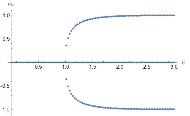
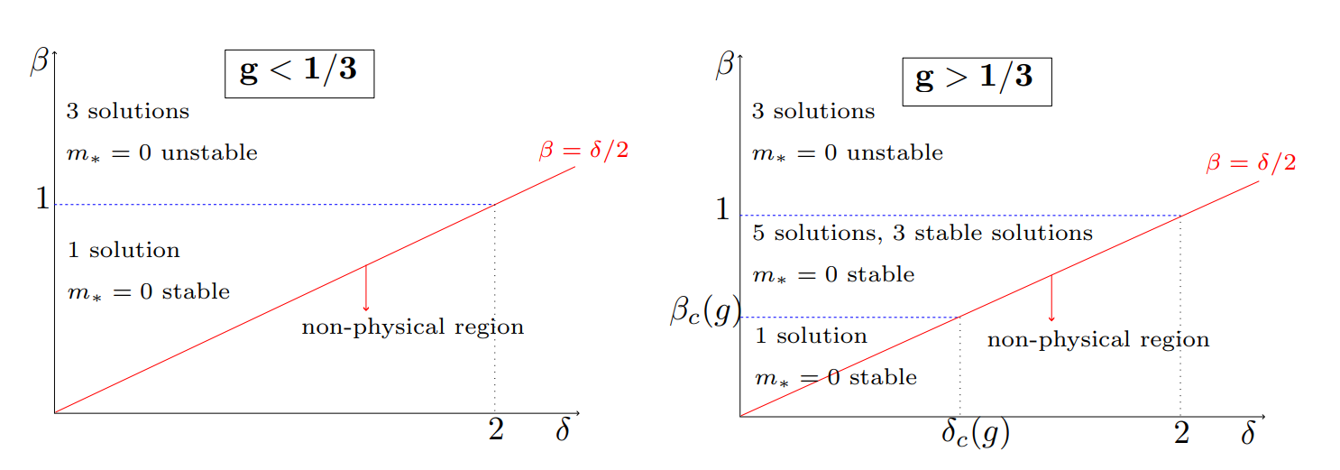
There are 1,3 or 5 solutions to (31), depending on the parameters β,g𝛽𝑔\beta,g. Since h=00h=0, the magnetization m=0subscript𝑚0m_{*}=0 is always a solution and indicates a paramagnetic phase. The other nonzero solutions m0subscript𝑚0m_{*}\neq 0 represent ferromagnetic states. Numerically solving (31) gives the pairs (β,m)𝛽subscript𝑚(\beta,m_{*}), shown in Fig. 3.

Refer to caption
(a) g<1/3𝑔13g<1/3: 1 or 3 solutions for msubscript𝑚m_{*}.
Refer to caption
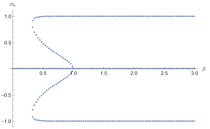
(b) g>1/3𝑔13g>1/3: 1,3 or 5 solutions for msubscript𝑚m_{*}.
Figure 3: Stationary magnetizations m(β)subscript𝑚𝛽m_{*}(\beta) for different values of g𝑔g. (Made using Mathematica version 13.1.0.0 [35].)

Since

H1(0)+H2(0)=4(β1)superscriptsubscript𝐻10superscriptsubscript𝐻204𝛽1H_{1}^{\prime}(0)+H_{2}^{\prime}(0)=4(\beta-1)

we have that m=0subscript𝑚0m_{*}=0 is stable for β1𝛽1\beta\leq 1 and unstable for β>1𝛽1\beta>1 (independent of g𝑔g) with critical inverse temperature βc=1subscript𝛽𝑐1\beta_{c}=1. An expansion of (31) near m0,β1formulae-sequencesubscript𝑚0𝛽1m_{*}\approx 0,\beta\approx 1 yields

m=±β11/3g +O((β1)32)subscript𝑚plus-or-minusβ11/3g 𝑂superscript𝛽132m_{*}=\pm\mathchoice{{\hbox{$\displaystyle\sqrt{\frac{\beta-1}{1/3-g}\,}$}\lower 0.4pt\hbox{\vrule height=13.88889pt,depth=-11.11116pt}}}{{\hbox{$\textstyle\sqrt{\frac{\beta-1}{1/3-g}\,}$}\lower 0.4pt\hbox{\vrule height=9.7222pt,depth=-7.7778pt}}}{{\hbox{$\scriptstyle\sqrt{\frac{\beta-1}{1/3-g}\,}$}\lower 0.4pt\hbox{\vrule height=6.94443pt,depth=-5.55557pt}}}{{\hbox{$\scriptscriptstyle\sqrt{\frac{\beta-1}{1/3-g}\,}$}\lower 0.4pt\hbox{\vrule height=6.94443pt,depth=-5.55557pt}}}+O\left((\beta-1)^{\frac{3}{2}}\right) (32)

As in equilibrium, m(ββc)zproportional-tosubscript𝑚superscript𝛽subscript𝛽𝑐𝑧m_{*}\propto(\beta-\beta_{c})^{z} with critical exponent z=12𝑧12z=\frac{1}{2} and m(gcg)yproportional-tosubscript𝑚superscriptsubscript𝑔𝑐𝑔𝑦m_{*}\propto(g_{c}-g)^{-y} where y=12𝑦12y=\frac{1}{2}. Furthermore, for g<13𝑔13g<\frac{1}{3}, the stationary magnetization m0subscript𝑚0m_{*}\approx 0 follows β1𝛽1\textstyle\sqrt{\beta-1\,}  for β>1𝛽1\beta>1, while for g>13𝑔13g>\frac{1}{3}, it grows like 1β1𝛽\textstyle\sqrt{1-\beta\,}  for β<1𝛽1\beta<1 (implying a second phase transition at gc=13subscript𝑔𝑐13g_{c}=\frac{1}{3}). This behaviour is also shown in Fig. 3.
Lastly, note that when δδc=2βc=2𝛿subscript𝛿𝑐2subscript𝛽𝑐2\delta\geq\delta_{c}=2\beta_{c}=2, then the constraint is β=δ21=βc𝛽𝛿21subscript𝛽𝑐\beta=\frac{\delta}{2}\geq 1=\beta_{c}, such that m=0subscript𝑚0m_{*}=0 is always unstable for δ>2𝛿2\delta>2. This introduces a critical δc=2subscript𝛿𝑐2\delta_{c}=2 in the phase diagrams.
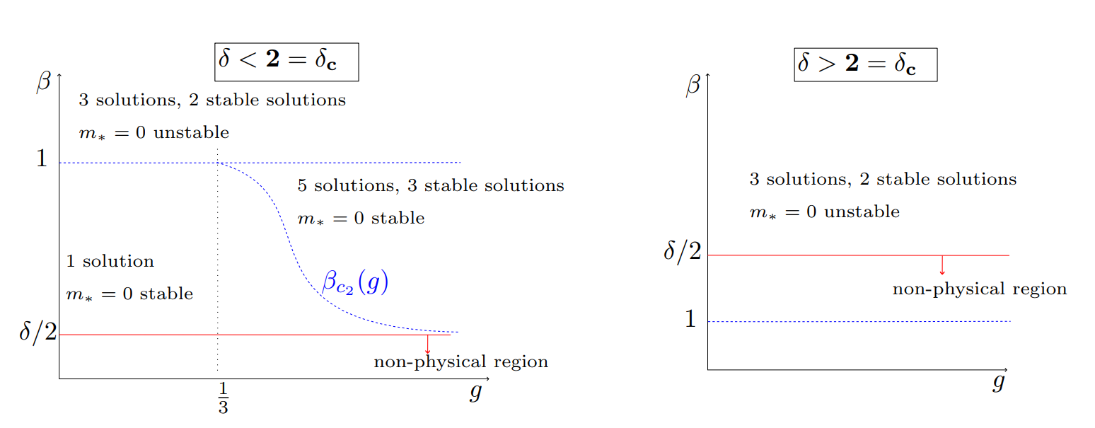
The phase diagrams in Figs. 45 combine all information for n=0𝑛0n=0.

Refer to caption
Figure 4: (g,β)𝑔𝛽(g,\beta) diagram for fixed δ𝛿\delta.
Refer to caption
Figure 5: (δ,β)𝛿𝛽(\delta,\beta) diagram for fixed g𝑔g.

The effect of the parameter g𝑔g is also visible from Figs. 45. For g<gc=1/3𝑔subscript𝑔𝑐13g<g_{c}=1/3, there are either 1 or 3 solutions, and the phase diagram looks qualitatively the same as for g=0𝑔0g=0. There is only one solution m=0subscript𝑚0m_{*}=0 (paramagnetic phase) for β<1𝛽1\beta<1 and three solutions for β>1𝛽1\beta>1, of which the two nonzero ones are stable (ferromagnetic phase).
When g>gc=13𝑔subscript𝑔𝑐13g>g_{c}=\frac{1}{3}, the phase diagram differs with 1,3 or 5 different values for msubscript𝑚m_{*} depending on β𝛽\beta. Five solutions of (31) appear for β[βc2(g),1]𝛽subscript𝛽subscript𝑐2𝑔1\beta\in[\beta_{c_{2}}(g),1] where βc2(g)subscript𝛽subscript𝑐2𝑔\beta_{c_{2}}(g) is obtained by solving the system of equations H(m)=0,H(m)=0formulae-sequence𝐻subscript𝑚0superscript𝐻subscript𝑚0H(m_{*})=0,H^{\prime}(m_{*})=0 simultaneously for the pair (βc2(g),m)subscript𝛽subscript𝑐2𝑔subscript𝑚(\beta_{c_{2}}(g),m_{*}). The two outer ferromagnetic branches in Fig. 3, as well as m=0subscript𝑚0m_{*}=0, are stable, while the two inner ferromagnetic branches are unstable. So by introducing g𝑔g, a coexistence appears between ferro- and paramagnetic phases.
Furthermore, m=0subscript𝑚0m_{*}=0 is the only solution when β<βc2(g)𝛽subscript𝛽subscript𝑐2𝑔\beta<\beta_{c_{2}}(g) while for β>βc=1𝛽subscript𝛽𝑐1\beta>\beta_{c}=1, three of the five solutions remain with an unstable m=0subscript𝑚0m_{*}=0 and stable m0subscript𝑚0m_{*}\neq 0.

4.2 n=1,g=0formulae-sequence𝑛1𝑔0n=1,\ g=0

For n=1𝑛1n=1, temperature-dependent kinetic effects are included in the spin-flip rates (3), which changes the phase diagram significantly. That is clearly a nonequilibrium effect. First, the stationary magnetization solves (29)

δtanhδ2ψ(m)=2βsinhβψ(m)mcoshβψ(m)msinhβψ(m)coshβψ(m),βδ2formulae-sequence𝛿𝛿2superscript𝜓subscript𝑚2𝛽𝛽superscript𝜓subscript𝑚subscript𝑚𝛽superscript𝜓subscript𝑚subscript𝑚𝛽superscript𝜓subscript𝑚𝛽superscript𝜓subscript𝑚𝛽𝛿2\delta\tanh{\frac{\delta}{2}\psi^{\prime}(m_{*})}=-2\beta\frac{\sinh{\beta\psi^{\prime}(m_{*})}-m_{*}\cosh{\beta\psi^{\prime}(m_{*})}}{m_{*}\sinh{\beta\psi^{\prime}(m_{*})}-\cosh{\beta\psi^{\prime}(m_{*})}},\qquad\beta\geq\frac{\delta}{2}\color[rgb]{0,0,0}\definecolor[named]{pgfstrokecolor}{rgb}{0,0,0}\pgfsys@color@gray@stroke{0}\pgfsys@color@gray@fill{0} (33)

which explicitly depends on δ𝛿\delta. Again, for h=00h=0, the magnetization m=0subscript𝑚0m_{*}=0 is always a solution.

We discuss here the case g=0𝑔0g=0 of (33); the case g0𝑔0g\neq 0 follows in the next subsection.
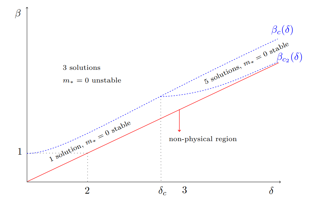
The phase diagram is given in Fig. 6 with 1,3 or 5 solutions depending on the values of β𝛽\beta and δ𝛿\delta. That differs from the n=0𝑛0n=0 case, which only has 1 or 3 solutions for g=0𝑔0g=0.
Solving H(0)=0superscript𝐻00H^{\prime}(0)=0 for the stability of m=0subscript𝑚0m_{*}=0, shows that it is stable for ββc(δ)𝛽subscript𝛽𝑐𝛿\beta\leq\beta_{c}(\delta) and unstable otherwise where

βc(δ)=1+1+δ2 2subscript𝛽𝑐𝛿11+δ2 2\beta_{c}(\delta)=\frac{1+\mathchoice{{\hbox{$\displaystyle\sqrt{1+\delta^{2}\,}$}\lower 0.4pt\hbox{\vrule height=8.74889pt,depth=-6.99915pt}}}{{\hbox{$\textstyle\sqrt{1+\delta^{2}\,}$}\lower 0.4pt\hbox{\vrule height=8.74889pt,depth=-6.99915pt}}}{{\hbox{$\scriptstyle\sqrt{1+\delta^{2}\,}$}\lower 0.4pt\hbox{\vrule height=6.14998pt,depth=-4.92001pt}}}{{\hbox{$\scriptscriptstyle\sqrt{1+\delta^{2}\,}$}\lower 0.4pt\hbox{\vrule height=4.7611pt,depth=-3.8089pt}}}}{2} (34)

As such, the critical temperature becomes δ𝛿\delta dependent, increases with the degree of nonequilibrium, and reduces to the equilibrium value βc(0)=1subscript𝛽𝑐01\beta_{c}(0)=1. Since in equation (34), βc(δ)1subscript𝛽𝑐𝛿1\beta_{c}(\delta)\geq 1 for all δ𝛿\delta, an island of stability opens up for the paramagnetic state, compared to the equilibrium and the n=0𝑛0n=0 case. Here we thus have unstable states that become stable due to the nonequilibrium driving.
In the two limits δ1much-less-than𝛿1\delta\ll 1 (close to equilibrium) and δ1much-greater-than𝛿1\delta\gg 1 (far from equilibrium), the critical temperatures reduce to, respectively,

βc1+δ24 for δ1, and βc1+δ2 for δ1formulae-sequencesubscript𝛽𝑐1superscript𝛿24 for 𝛿much-less-than1 and subscript𝛽𝑐1𝛿2 for 𝛿much-greater-than1\beta_{c}\approx 1+\frac{\delta^{2}}{4}\text{ for }\delta\ll 1,\quad\text{ and }\qquad\beta_{c}\approx\frac{1+\delta}{2}\text{ for }\delta\gg 1

i.e., we get quadratic corrections in δ𝛿\delta close to equilibrium while βc(δ)subscript𝛽𝑐𝛿\beta_{c}(\delta) grows linear in δ𝛿\delta for a large nonequilibrium driving. Finally, the magnetization near the critical temperature βc(δ)subscript𝛽𝑐𝛿\beta_{c}(\delta) equals

m=±24(1+δ2)(ββc(δ))(4+δ2)+(4δ2)1+δ2  +O((ββc(δ))32)subscript𝑚plus-or-minus24(1+δ2)(ββc(δ))(4+δ2)+(4δ2)1+δ2  𝑂superscript𝛽subscript𝛽𝑐𝛿32m_{*}=\pm\mathchoice{{\hbox{$\displaystyle\sqrt{\frac{24(1+\delta^{2})(\beta-\beta_{c}(\delta))}{(4+\delta^{2})+(4-\delta^{2})\mathchoice{{\hbox{$\displaystyle\sqrt{1+\delta^{2}\,}$}\lower 0.4pt\hbox{\vrule height=8.74889pt,depth=-6.99915pt}}}{{\hbox{$\textstyle\sqrt{1+\delta^{2}\,}$}\lower 0.4pt\hbox{\vrule height=8.74889pt,depth=-6.99915pt}}}{{\hbox{$\scriptstyle\sqrt{1+\delta^{2}\,}$}\lower 0.4pt\hbox{\vrule height=6.14998pt,depth=-4.92001pt}}}{{\hbox{$\scriptscriptstyle\sqrt{1+\delta^{2}\,}$}\lower 0.4pt\hbox{\vrule height=4.7611pt,depth=-3.8089pt}}}}\,}$}\lower 0.4pt\hbox{\vrule height=16.87332pt,depth=-13.49872pt}}}{{\hbox{$\textstyle\sqrt{\frac{24(1+\delta^{2})(\beta-\beta_{c}(\delta))}{(4+\delta^{2})+(4-\delta^{2})\mathchoice{{\hbox{$\displaystyle\sqrt{1+\delta^{2}\,}$}\lower 0.4pt\hbox{\vrule height=6.1242pt,depth=-4.8994pt}}}{{\hbox{$\textstyle\sqrt{1+\delta^{2}\,}$}\lower 0.4pt\hbox{\vrule height=6.1242pt,depth=-4.8994pt}}}{{\hbox{$\scriptstyle\sqrt{1+\delta^{2}\,}$}\lower 0.4pt\hbox{\vrule height=4.305pt,depth=-3.44402pt}}}{{\hbox{$\scriptscriptstyle\sqrt{1+\delta^{2}\,}$}\lower 0.4pt\hbox{\vrule height=3.33276pt,depth=-2.66623pt}}}}\,}$}\lower 0.4pt\hbox{\vrule height=11.84996pt,depth=-9.48001pt}}}{{\hbox{$\scriptstyle\sqrt{\frac{24(1+\delta^{2})(\beta-\beta_{c}(\delta))}{(4+\delta^{2})+(4-\delta^{2})\mathchoice{{\hbox{$\displaystyle\sqrt{1+\delta^{2}\,}$}\lower 0.4pt\hbox{\vrule height=4.37444pt,depth=-3.49957pt}}}{{\hbox{$\textstyle\sqrt{1+\delta^{2}\,}$}\lower 0.4pt\hbox{\vrule height=4.37444pt,depth=-3.49957pt}}}{{\hbox{$\scriptstyle\sqrt{1+\delta^{2}\,}$}\lower 0.4pt\hbox{\vrule height=3.07498pt,depth=-2.46pt}}}{{\hbox{$\scriptscriptstyle\sqrt{1+\delta^{2}\,}$}\lower 0.4pt\hbox{\vrule height=2.38054pt,depth=-1.90445pt}}}}\,}$}\lower 0.4pt\hbox{\vrule height=9.01663pt,depth=-7.21335pt}}}{{\hbox{$\scriptscriptstyle\sqrt{\frac{24(1+\delta^{2})(\beta-\beta_{c}(\delta))}{(4+\delta^{2})+(4-\delta^{2})\mathchoice{{\hbox{$\displaystyle\sqrt{1+\delta^{2}\,}$}\lower 0.4pt\hbox{\vrule height=4.37444pt,depth=-3.49957pt}}}{{\hbox{$\textstyle\sqrt{1+\delta^{2}\,}$}\lower 0.4pt\hbox{\vrule height=4.37444pt,depth=-3.49957pt}}}{{\hbox{$\scriptstyle\sqrt{1+\delta^{2}\,}$}\lower 0.4pt\hbox{\vrule height=3.07498pt,depth=-2.46pt}}}{{\hbox{$\scriptscriptstyle\sqrt{1+\delta^{2}\,}$}\lower 0.4pt\hbox{\vrule height=2.38054pt,depth=-1.90445pt}}}}\,}$}\lower 0.4pt\hbox{\vrule height=9.01663pt,depth=-7.21335pt}}}+O\left((\beta-\beta_{c}(\delta))^{\frac{3}{2}}\right) (35)

The denominator in (35) is positive for δ<δc=22 𝛿subscript𝛿𝑐22 \delta<\delta_{c}=2\mathchoice{{\hbox{$\displaystyle\sqrt{2\,}$}\lower 0.4pt\hbox{\vrule height=6.44444pt,depth=-5.15558pt}}}{{\hbox{$\textstyle\sqrt{2\,}$}\lower 0.4pt\hbox{\vrule height=6.44444pt,depth=-5.15558pt}}}{{\hbox{$\scriptstyle\sqrt{2\,}$}\lower 0.4pt\hbox{\vrule height=4.51111pt,depth=-3.6089pt}}}{{\hbox{$\scriptscriptstyle\sqrt{2\,}$}\lower 0.4pt\hbox{\vrule height=3.22221pt,depth=-2.57779pt}}} and negative otherwise. Thus, when δ<22 𝛿22 \delta<2\mathchoice{{\hbox{$\displaystyle\sqrt{2\,}$}\lower 0.4pt\hbox{\vrule height=6.44444pt,depth=-5.15558pt}}}{{\hbox{$\textstyle\sqrt{2\,}$}\lower 0.4pt\hbox{\vrule height=6.44444pt,depth=-5.15558pt}}}{{\hbox{$\scriptstyle\sqrt{2\,}$}\lower 0.4pt\hbox{\vrule height=4.51111pt,depth=-3.6089pt}}}{{\hbox{$\scriptscriptstyle\sqrt{2\,}$}\lower 0.4pt\hbox{\vrule height=3.22221pt,depth=-2.57779pt}}}, the magnetization behaves like ββc(δ)𝛽subscript𝛽𝑐𝛿\textstyle\sqrt{\beta-\beta_{c}(\delta)\,}  for β>βc(δ)𝛽subscript𝛽𝑐𝛿\beta>\beta_{c}(\delta), while for δ>22 𝛿22 \delta>2\mathchoice{{\hbox{$\displaystyle\sqrt{2\,}$}\lower 0.4pt\hbox{\vrule height=6.44444pt,depth=-5.15558pt}}}{{\hbox{$\textstyle\sqrt{2\,}$}\lower 0.4pt\hbox{\vrule height=6.44444pt,depth=-5.15558pt}}}{{\hbox{$\scriptstyle\sqrt{2\,}$}\lower 0.4pt\hbox{\vrule height=4.51111pt,depth=-3.6089pt}}}{{\hbox{$\scriptscriptstyle\sqrt{2\,}$}\lower 0.4pt\hbox{\vrule height=3.22221pt,depth=-2.57779pt}}}, it behaves like βc(δ)βsubscript𝛽𝑐𝛿𝛽\textstyle\sqrt{\beta_{c}(\delta)-\beta\,}  for β<βc(δ)𝛽subscript𝛽𝑐𝛿\beta<\beta_{c}(\delta). As before, the critical exponent for β𝛽\beta equals z=12𝑧12z=\frac{1}{2}, while m(δδc)γproportional-tosubscript𝑚superscript𝛿subscript𝛿𝑐𝛾m_{*}\propto(\delta-\delta_{c})^{-\gamma} with γ=12𝛾12\gamma=\frac{1}{2}

Refer to caption
Figure 6: Phase diagram, with n=1𝑛1n=1, h=00h=0 and g=0𝑔0g=0. The strip between the upper dotted blue line and the red line is the island of stability for m=0subscript𝑚0m_{*}=0.

For δ<δc=22 𝛿subscript𝛿𝑐22 \delta<\delta_{c}=2\mathchoice{{\hbox{$\displaystyle\sqrt{2\,}$}\lower 0.4pt\hbox{\vrule height=6.44444pt,depth=-5.15558pt}}}{{\hbox{$\textstyle\sqrt{2\,}$}\lower 0.4pt\hbox{\vrule height=6.44444pt,depth=-5.15558pt}}}{{\hbox{$\scriptstyle\sqrt{2\,}$}\lower 0.4pt\hbox{\vrule height=4.51111pt,depth=-3.6089pt}}}{{\hbox{$\scriptscriptstyle\sqrt{2\,}$}\lower 0.4pt\hbox{\vrule height=3.22221pt,depth=-2.57779pt}}}, the magnetization m=0subscript𝑚0m_{*}=0 is the only solution for β<βc(δ)𝛽subscript𝛽𝑐𝛿\beta<\beta_{c}(\delta) and two extra stable ferromagnetic solutions m0subscript𝑚0m_{*}\neq 0 arise when β>βc(δ)𝛽subscript𝛽𝑐𝛿\beta>\beta_{c}(\delta). This result is similar to the n=0,g<13formulae-sequence𝑛0𝑔13n=0,g<\frac{1}{3} case from before.
On the other hand, if δ>δc=22 𝛿subscript𝛿𝑐22 \delta>\delta_{c}=2\mathchoice{{\hbox{$\displaystyle\sqrt{2\,}$}\lower 0.4pt\hbox{\vrule height=6.44444pt,depth=-5.15558pt}}}{{\hbox{$\textstyle\sqrt{2\,}$}\lower 0.4pt\hbox{\vrule height=6.44444pt,depth=-5.15558pt}}}{{\hbox{$\scriptstyle\sqrt{2\,}$}\lower 0.4pt\hbox{\vrule height=4.51111pt,depth=-3.6089pt}}}{{\hbox{$\scriptscriptstyle\sqrt{2\,}$}\lower 0.4pt\hbox{\vrule height=3.22221pt,depth=-2.57779pt}}}, a new critical temperature βc2(δ)βc(δ)subscript𝛽subscript𝑐2𝛿subscript𝛽𝑐𝛿\beta_{c_{2}}(\delta)\leq\beta_{c}(\delta) appears for which m=0subscript𝑚0m_{*}=0 is the only solution when ββc2(δ)𝛽subscript𝛽subscript𝑐2𝛿\beta\leq\beta_{c_{2}}(\delta) (pure paramagnetic) and 5 solutions for βc2(δ)<β<βc(δ)subscript𝛽subscript𝑐2𝛿𝛽subscript𝛽𝑐𝛿\beta_{c_{2}}(\delta)<\beta<\beta_{c}(\delta) (paramagentic and ferromagnetic phase coexistence). Two of these ferromagnetic states are stable, while m=0subscript𝑚0m_{*}=0 is only stable for β<βc(δ)𝛽subscript𝛽𝑐𝛿\beta<\beta_{c}(\delta). Note that this behaviour is very similar to the g>13𝑔13g>\frac{1}{3} case from the previous section. The major difference, however, is that the critical temperatures are δ𝛿\delta–dependent.
As before, the second critical temperature βc2(δ)subscript𝛽subscript𝑐2𝛿\beta_{c_{2}}(\delta) is obtained from the equations H(m)=0,H(m)=0formulae-sequence𝐻subscript𝑚0superscript𝐻subscript𝑚0H(m_{*})=0,H^{\prime}(m_{*})=0. It intersects βc(δ)subscript𝛽𝑐𝛿\beta_{c}(\delta) at δ=δc𝛿subscript𝛿𝑐\delta=\delta_{c}, and moves asymptotically towards δ2𝛿2\frac{\delta}{2} for large δ𝛿\delta, but it never crosses that line.

4.3 n=1,g0formulae-sequence𝑛1𝑔0n=1,\ g\neq 0

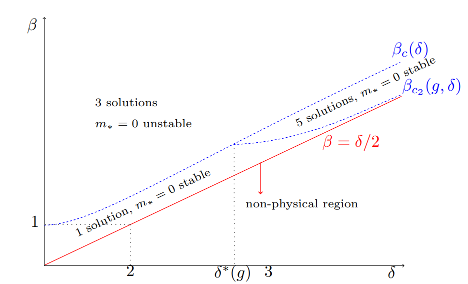
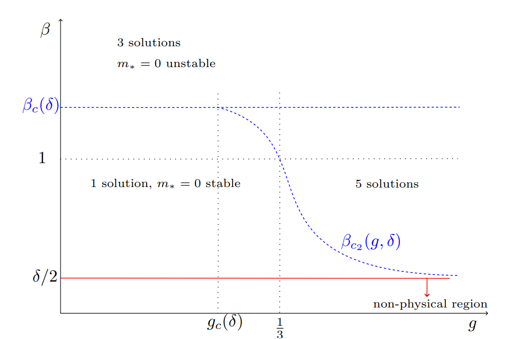
The biggest changes for g0𝑔0g\neq 0 and n=1𝑛1n=1, is that the critical value gc(δ)subscript𝑔𝑐𝛿g_{c}(\delta) (which was the constant 1313\frac{1}{3} before) becomes δ𝛿\delta-dependent and the second critical inverse temperature βc2(g,δ)subscript𝛽subscript𝑐2𝑔𝛿\beta_{c_{2}}(g,\delta) becomes a function of both g𝑔g and δ𝛿\delta. We depict the phase diagrams in Figs 78, which have a form similar to the case n=0,g0formulae-sequence𝑛0𝑔0n=0,g\neq 0.
As before, the critical value gc(δ)subscript𝑔𝑐𝛿g_{c}(\delta) follows from expanding m0,ββc(δ)formulae-sequencesubscript𝑚0𝛽subscript𝛽𝑐𝛿m_{*}\approx 0,\beta\approx\beta_{c}(\delta) in (33)

m=±12(1+δ2)(ββc(δ))6(1+1+δ2 )(gc(δ)g) +O((ββc(δ))32)subscript𝑚plus-or-minus12(1+δ2)(ββc(δ))6(1+1+δ2 )(gc(δ)g) 𝑂superscript𝛽subscript𝛽𝑐𝛿32m_{*}=\pm\mathchoice{{\hbox{$\displaystyle\sqrt{\frac{12(1+\delta^{2})(\beta-\beta_{c}(\delta))}{6(1+\mathchoice{{\hbox{$\displaystyle\sqrt{1+\delta^{2}\,}$}\lower 0.4pt\hbox{\vrule height=8.74889pt,depth=-6.99915pt}}}{{\hbox{$\textstyle\sqrt{1+\delta^{2}\,}$}\lower 0.4pt\hbox{\vrule height=8.74889pt,depth=-6.99915pt}}}{{\hbox{$\scriptstyle\sqrt{1+\delta^{2}\,}$}\lower 0.4pt\hbox{\vrule height=6.14998pt,depth=-4.92001pt}}}{{\hbox{$\scriptscriptstyle\sqrt{1+\delta^{2}\,}$}\lower 0.4pt\hbox{\vrule height=4.7611pt,depth=-3.8089pt}}})(g_{c}(\delta)-g)}\,}$}\lower 0.4pt\hbox{\vrule height=16.87332pt,depth=-13.49872pt}}}{{\hbox{$\textstyle\sqrt{\frac{12(1+\delta^{2})(\beta-\beta_{c}(\delta))}{6(1+\mathchoice{{\hbox{$\displaystyle\sqrt{1+\delta^{2}\,}$}\lower 0.4pt\hbox{\vrule height=6.1242pt,depth=-4.8994pt}}}{{\hbox{$\textstyle\sqrt{1+\delta^{2}\,}$}\lower 0.4pt\hbox{\vrule height=6.1242pt,depth=-4.8994pt}}}{{\hbox{$\scriptstyle\sqrt{1+\delta^{2}\,}$}\lower 0.4pt\hbox{\vrule height=4.305pt,depth=-3.44402pt}}}{{\hbox{$\scriptscriptstyle\sqrt{1+\delta^{2}\,}$}\lower 0.4pt\hbox{\vrule height=3.33276pt,depth=-2.66623pt}}})(g_{c}(\delta)-g)}\,}$}\lower 0.4pt\hbox{\vrule height=11.83708pt,depth=-9.46971pt}}}{{\hbox{$\scriptstyle\sqrt{\frac{12(1+\delta^{2})(\beta-\beta_{c}(\delta))}{6(1+\mathchoice{{\hbox{$\displaystyle\sqrt{1+\delta^{2}\,}$}\lower 0.4pt\hbox{\vrule height=4.37444pt,depth=-3.49957pt}}}{{\hbox{$\textstyle\sqrt{1+\delta^{2}\,}$}\lower 0.4pt\hbox{\vrule height=4.37444pt,depth=-3.49957pt}}}{{\hbox{$\scriptstyle\sqrt{1+\delta^{2}\,}$}\lower 0.4pt\hbox{\vrule height=3.07498pt,depth=-2.46pt}}}{{\hbox{$\scriptscriptstyle\sqrt{1+\delta^{2}\,}$}\lower 0.4pt\hbox{\vrule height=2.38054pt,depth=-1.90445pt}}})(g_{c}(\delta)-g)}\,}$}\lower 0.4pt\hbox{\vrule height=8.8233pt,depth=-7.05867pt}}}{{\hbox{$\scriptscriptstyle\sqrt{\frac{12(1+\delta^{2})(\beta-\beta_{c}(\delta))}{6(1+\mathchoice{{\hbox{$\displaystyle\sqrt{1+\delta^{2}\,}$}\lower 0.4pt\hbox{\vrule height=4.37444pt,depth=-3.49957pt}}}{{\hbox{$\textstyle\sqrt{1+\delta^{2}\,}$}\lower 0.4pt\hbox{\vrule height=4.37444pt,depth=-3.49957pt}}}{{\hbox{$\scriptstyle\sqrt{1+\delta^{2}\,}$}\lower 0.4pt\hbox{\vrule height=3.07498pt,depth=-2.46pt}}}{{\hbox{$\scriptscriptstyle\sqrt{1+\delta^{2}\,}$}\lower 0.4pt\hbox{\vrule height=2.38054pt,depth=-1.90445pt}}})(g_{c}(\delta)-g)}\,}$}\lower 0.4pt\hbox{\vrule height=8.8233pt,depth=-7.05867pt}}}+O\left((\beta-\beta_{c}(\delta))^{\frac{3}{2}}\right) (36)

with

gc(δ)=13δ2(1+δ2 1)12(1+1+δ2 )subscript𝑔𝑐𝛿13superscript𝛿21+δ2 11211+δ2 g_{c}(\delta)=\frac{1}{3}-\frac{\delta^{2}(\mathchoice{{\hbox{$\displaystyle\sqrt{1+\delta^{2}\,}$}\lower 0.4pt\hbox{\vrule height=8.74889pt,depth=-6.99915pt}}}{{\hbox{$\textstyle\sqrt{1+\delta^{2}\,}$}\lower 0.4pt\hbox{\vrule height=8.74889pt,depth=-6.99915pt}}}{{\hbox{$\scriptstyle\sqrt{1+\delta^{2}\,}$}\lower 0.4pt\hbox{\vrule height=6.14998pt,depth=-4.92001pt}}}{{\hbox{$\scriptscriptstyle\sqrt{1+\delta^{2}\,}$}\lower 0.4pt\hbox{\vrule height=4.7611pt,depth=-3.8089pt}}}-1)}{12(1+\mathchoice{{\hbox{$\displaystyle\sqrt{1+\delta^{2}\,}$}\lower 0.4pt\hbox{\vrule height=8.74889pt,depth=-6.99915pt}}}{{\hbox{$\textstyle\sqrt{1+\delta^{2}\,}$}\lower 0.4pt\hbox{\vrule height=8.74889pt,depth=-6.99915pt}}}{{\hbox{$\scriptstyle\sqrt{1+\delta^{2}\,}$}\lower 0.4pt\hbox{\vrule height=6.14998pt,depth=-4.92001pt}}}{{\hbox{$\scriptscriptstyle\sqrt{1+\delta^{2}\,}$}\lower 0.4pt\hbox{\vrule height=4.7611pt,depth=-3.8089pt}}})} (37)

which is always smaller than 1313\frac{1}{3}. The function gc(δ)subscript𝑔𝑐𝛿g_{c}(\delta) is decrease for δ>0𝛿0\delta>0 and becomes zero at gc(δc)=gc(22 )=0subscript𝑔𝑐subscript𝛿𝑐subscript𝑔𝑐22 0g_{c}(\delta_{c})=g_{c}(2\mathchoice{{\hbox{$\displaystyle\sqrt{2\,}$}\lower 0.4pt\hbox{\vrule height=6.44444pt,depth=-5.15558pt}}}{{\hbox{$\textstyle\sqrt{2\,}$}\lower 0.4pt\hbox{\vrule height=6.44444pt,depth=-5.15558pt}}}{{\hbox{$\scriptstyle\sqrt{2\,}$}\lower 0.4pt\hbox{\vrule height=4.51111pt,depth=-3.6089pt}}}{{\hbox{$\scriptscriptstyle\sqrt{2\,}$}\lower 0.4pt\hbox{\vrule height=3.22221pt,depth=-2.57779pt}}})=0. Furthermore, for small δ𝛿\delta (close to equilibrium), one finds

gc(δ)13δ448 for δ1subscript𝑔𝑐𝛿13superscript𝛿448 for 𝛿much-less-than1g_{c}(\delta)\approx\frac{1}{3}-\frac{\delta^{4}}{48}\text{ for }\delta\ll 1

I.e., the corrections with respect to equilibrium are of fourth order in δ𝛿\delta. From (36), for g<gc(δ)𝑔subscript𝑔𝑐𝛿g<g_{c}(\delta), the magnetization behaves like ββc(δ)𝛽subscript𝛽𝑐𝛿\textstyle\sqrt{\beta-\beta_{c}(\delta)\,}  for β>βc(δ)𝛽subscript𝛽𝑐𝛿\beta>\beta_{c}(\delta), while for g>gc(δ)𝑔subscript𝑔𝑐𝛿g>g_{c}(\delta), it follows βc(δ)βsubscript𝛽𝑐𝛿𝛽\textstyle\sqrt{\beta_{c}(\delta)-\beta\,}  for β<βc(δ)𝛽subscript𝛽𝑐𝛿\beta<\beta_{c}(\delta). Furthermore, the critical exponents remain the same as before. Finally, by inverting (37), the critical δcsubscript𝛿𝑐\delta_{c} as a function of g𝑔g is obtained as

δ(g)=213g+13g  superscript𝛿𝑔213g+13g  \delta^{*}(g)=2\mathchoice{{\hbox{$\displaystyle\sqrt{1-3g+\mathchoice{{\hbox{$\displaystyle\sqrt{1-3g\,}$}\lower 0.4pt\hbox{\vrule height=6.44444pt,depth=-5.15558pt}}}{{\hbox{$\textstyle\sqrt{1-3g\,}$}\lower 0.4pt\hbox{\vrule height=6.44444pt,depth=-5.15558pt}}}{{\hbox{$\scriptstyle\sqrt{1-3g\,}$}\lower 0.4pt\hbox{\vrule height=4.51111pt,depth=-3.6089pt}}}{{\hbox{$\scriptscriptstyle\sqrt{1-3g\,}$}\lower 0.4pt\hbox{\vrule height=3.22221pt,depth=-2.57779pt}}}\,}$}\lower 0.4pt\hbox{\vrule height=6.44444pt,depth=-5.15558pt}}}{{\hbox{$\textstyle\sqrt{1-3g+\mathchoice{{\hbox{$\displaystyle\sqrt{1-3g\,}$}\lower 0.4pt\hbox{\vrule height=6.44444pt,depth=-5.15558pt}}}{{\hbox{$\textstyle\sqrt{1-3g\,}$}\lower 0.4pt\hbox{\vrule height=6.44444pt,depth=-5.15558pt}}}{{\hbox{$\scriptstyle\sqrt{1-3g\,}$}\lower 0.4pt\hbox{\vrule height=4.51111pt,depth=-3.6089pt}}}{{\hbox{$\scriptscriptstyle\sqrt{1-3g\,}$}\lower 0.4pt\hbox{\vrule height=3.22221pt,depth=-2.57779pt}}}\,}$}\lower 0.4pt\hbox{\vrule height=6.44444pt,depth=-5.15558pt}}}{{\hbox{$\scriptstyle\sqrt{1-3g+\mathchoice{{\hbox{$\displaystyle\sqrt{1-3g\,}$}\lower 0.4pt\hbox{\vrule height=4.51111pt,depth=-3.6089pt}}}{{\hbox{$\textstyle\sqrt{1-3g\,}$}\lower 0.4pt\hbox{\vrule height=4.51111pt,depth=-3.6089pt}}}{{\hbox{$\scriptstyle\sqrt{1-3g\,}$}\lower 0.4pt\hbox{\vrule height=3.15778pt,depth=-2.52625pt}}}{{\hbox{$\scriptscriptstyle\sqrt{1-3g\,}$}\lower 0.4pt\hbox{\vrule height=2.25555pt,depth=-1.80446pt}}}\,}$}\lower 0.4pt\hbox{\vrule height=4.51111pt,depth=-3.6089pt}}}{{\hbox{$\scriptscriptstyle\sqrt{1-3g+\mathchoice{{\hbox{$\displaystyle\sqrt{1-3g\,}$}\lower 0.4pt\hbox{\vrule height=3.22221pt,depth=-2.57779pt}}}{{\hbox{$\textstyle\sqrt{1-3g\,}$}\lower 0.4pt\hbox{\vrule height=3.22221pt,depth=-2.57779pt}}}{{\hbox{$\scriptstyle\sqrt{1-3g\,}$}\lower 0.4pt\hbox{\vrule height=2.25555pt,depth=-1.80446pt}}}{{\hbox{$\scriptscriptstyle\sqrt{1-3g\,}$}\lower 0.4pt\hbox{\vrule height=1.6111pt,depth=-1.2889pt}}}\,}$}\lower 0.4pt\hbox{\vrule height=3.22221pt,depth=-2.57779pt}}}

The second critical temperature βc2(g,δ)subscript𝛽subscript𝑐2𝑔𝛿\beta_{c_{2}}(g,\delta) only exists when δ>δ(g)𝛿superscript𝛿𝑔\delta>\delta^{*}(g), intersects βc(δ)subscript𝛽𝑐𝛿\beta_{c}(\delta) at δ(g)superscript𝛿𝑔\delta^{*}(g) and moves asymptotically to δ2𝛿2\frac{\delta}{2} as δ𝛿\delta\uparrow\infty for all g𝑔g.

Refer to caption
Figure 7: (δ𝛿\delta, β)\beta) diagram for fixed g<1/3𝑔13g<1/3. The region between βc(δ)subscript𝛽𝑐𝛿\beta_{c}(\delta) and the red line represents the region of stability for m=0subscript𝑚0m_{*}=0.
Refer to caption
Figure 8: (g,β)𝑔𝛽(g,\beta) diagram for fixed δ𝛿\delta.

Qualitatively, compared to the case n=0𝑛0n=0, the phase diagrams in Figs. 7 and 8 move with δ𝛿\delta, and the critical values βc=1subscript𝛽𝑐1\beta_{c}=1 and gc=1/3subscript𝑔𝑐13g_{c}=1/3 are changed into δ𝛿\delta-dependent functions βc(δ)subscript𝛽𝑐𝛿\beta_{c}(\delta) and gc(δ)subscript𝑔𝑐𝛿g_{c}(\delta). As before, we distinguish between three different phases: pure paramagnetic m=0subscript𝑚0m_{*}=0 for β<βc2(g,δ)𝛽subscript𝛽subscript𝑐2𝑔𝛿\beta<\beta_{c_{2}}(g,\delta), pure ferromagnetic m0subscript𝑚0m_{*}\neq 0 for β>βc(δ)𝛽subscript𝛽𝑐𝛿\beta>\beta_{c}(\delta) and a stable ferro- and paramagnetic phase in between these critical temperatures.

5 Heat capacity

This section gives the specific heat for the macroscopic two-temperature Curie-Weiss model and discusses its properties We refer to Section 2.3 for the finite setup. The derivation of the main formula comes in Section 6.

Since the heat capacity is an extensive quantity, Cab(N)Nproportional-tosuperscriptsubscript𝐶𝑎𝑏𝑁𝑁C_{ab}^{(N)}\propto N when N𝑁N\uparrow\infty, the quantity of interest is the specific heat (heat capacity per spin),

cab:=limNCab(N)N=limN1NkBβb2Va(N)βbNsassignsubscript𝑐𝑎𝑏subscript𝑁superscriptsubscript𝐶𝑎𝑏𝑁𝑁subscript𝑁1𝑁subscript𝑘𝐵superscriptsubscript𝛽𝑏2subscriptsuperscriptdelimited-⟨⟩subscriptsuperscript𝑉𝑁𝑎subscript𝛽𝑏𝑠𝑁c_{ab}:=\lim_{N\uparrow\infty}\frac{C_{ab}^{(N)}}{N}=\lim_{N\uparrow\infty}\frac{1}{N}k_{B}\beta_{b}^{2}\Big{\langle}\frac{\partial V^{(N)}_{a}}{\partial\beta_{b}}\Big{\rangle}^{s}_{N} (38)

where we have used (15) for the characterization of the thermal response in terms of the quasipotential.

Main result: The specific heat of the two-temperature Curie-Weiss model in a stable phase with magnetization msubscript𝑚m_{*} is given by

cab=kBβb2Jmβbψ′′(m)Ha(m)+ψ(m)Ha(m)H(m)subscript𝑐𝑎𝑏subscript𝑘𝐵superscriptsubscript𝛽𝑏2𝐽subscript𝑚subscript𝛽𝑏superscript𝜓′′subscript𝑚subscript𝐻𝑎subscript𝑚superscript𝜓subscript𝑚subscriptsuperscript𝐻𝑎subscript𝑚superscript𝐻subscript𝑚c_{ab}=k_{B}\beta_{b}^{2}J\frac{\partial m_{*}}{\partial\beta_{b}}\frac{\psi^{\prime\prime}(m_{*})H_{a}(m_{*})+\psi^{\prime}(m_{*})H^{\prime}_{a}(m_{*})}{H^{\prime}(m_{*})} (39)

We refer to (1) and (20) for the definitions of the functions ψ𝜓\psi and the Hasubscript𝐻𝑎H_{a}. Note that in equilibrium (β1=β2subscript𝛽1subscript𝛽2\beta_{1}=\beta_{2}), Ha(m)=0subscript𝐻𝑎subscript𝑚0H_{a}(m_{*})=0 and 2Ha=H2subscript𝐻𝑎𝐻2H_{a}=H.
Formula (39) is derived in Section 6. We first focus on its properties and what modifications arise compared to the equilibrium situation.

5.1 Close to equilibrium

In equilibrium when Jβ2=Jβ1=Jβeq=β𝐽subscript𝛽2𝐽subscript𝛽1𝐽subscript𝛽eq𝛽J\beta_{2}=J\beta_{1}=J\beta_{\text{eq}}=\beta, and m=meqsubscript𝑚subscript𝑚eqm_{*}=m_{\text{eq}}, the specific heat capacities (39) reduce to

cabeq=kBJ2βb2ψ(meq)meqβb=kB4β2ψ(meq)meqβsuperscriptsubscript𝑐𝑎𝑏eqsubscript𝑘𝐵𝐽2superscriptsubscript𝛽𝑏2superscript𝜓subscript𝑚eqsubscript𝑚eqsubscript𝛽𝑏subscript𝑘𝐵4superscript𝛽2superscript𝜓subscript𝑚eqsubscript𝑚eq𝛽c_{ab}^{\text{eq}}=\frac{k_{B}J}{2}\beta_{b}^{2}\psi^{\prime}(m_{\text{eq}})\frac{\partial m_{\text{eq}}}{\partial\beta_{b}}=\frac{k_{B}}{4}\beta^{2}\psi^{\prime}(m_{\text{eq}})\frac{\partial m_{\text{eq}}}{\partial\beta} (40)

in terms of the dimensionless β𝛽\beta. There is no dependence on a,b𝑎𝑏a,b, and all heat capacities agree. By adding the cabeqsuperscriptsubscript𝑐𝑎𝑏eqc_{ab}^{\text{eq}}, one gets the equilibrium result,

ceq=kbβ2ψ(meq)meqβsubscript𝑐eqsubscript𝑘𝑏superscript𝛽2superscript𝜓subscript𝑚eqsubscript𝑚eq𝛽c_{\text{eq}}=k_{b}\beta^{2}\psi^{\prime}(m_{\text{eq}})\frac{\partial m_{\text{eq}}}{\partial\beta} (41)

As a reminder, for the n=h=0𝑛0n=h=0 case, the specific heats (40) reduce to

cabeq={0,if β<118(13g)kB,if β>1subscriptsuperscript𝑐eq𝑎𝑏cases0if β<11813𝑔subscript𝑘𝐵if β>1c^{\text{eq}}_{ab}=\begin{cases}0,&\text{if $\beta<1$}\\ \frac{1}{8(\frac{1}{3}-g)}k_{B},&\text{if $\beta>1$}\end{cases} (42)

where we used (32). At fixed g13𝑔13g\neq\frac{1}{3}, the heat capacity (42) makes a finite jump as β1𝛽1\beta\to 1 (critical exponent α=0𝛼0\alpha=0, [3]). Furthermore, still in equilibrium, a divergence of the form (13g)νsuperscript13𝑔𝜈(\frac{1}{3}-g)^{-\nu} with critical exponent ν=1𝜈1\nu=1 takes place at g=1/3𝑔13g=1/3. As we will see below, the critical exponents change when going to nonequilibrium.

To describe the close-to-equilibrium behavior, we write β1=1J(βδ2),β2=1J(β+δ2)formulae-sequencesubscript𝛽11𝐽𝛽𝛿2subscript𝛽21𝐽𝛽𝛿2\beta_{1}=\frac{1}{J}(\beta-\frac{\delta}{2}),\beta_{2}=\frac{1}{J}(\beta+\frac{\delta}{2}), and, for fixed β𝛽\beta, we expand in small δ𝛿\delta

Hasubscript𝐻𝑎\displaystyle H_{a} =Heq+(1)a+1δ2[nβHeqSeqψ(m)]+O(δ2),a=1,2formulae-sequenceabsentsubscript𝐻eqsuperscript1𝑎1𝛿2delimited-[]𝑛𝛽subscript𝐻eqsubscript𝑆eqsuperscript𝜓subscript𝑚𝑂superscript𝛿2𝑎12\displaystyle=H_{\text{eq}}+(-1)^{a+1}\frac{\delta}{2}\Big{[}\frac{n}{\beta}H_{\text{eq}}-S_{\text{eq}}\psi^{\prime}(m_{*})\Big{]}+O(\delta^{2}),\qquad a=1,2
J2βb2superscript𝐽2superscriptsubscript𝛽𝑏2\displaystyle J^{2}\beta_{b}^{2} =β2+(1)bβδ+O(δ2),b=1,2formulae-sequenceabsentsuperscript𝛽2superscript1𝑏𝛽𝛿𝑂superscript𝛿2𝑏12\displaystyle=\beta^{2}+(-1)^{b}\,\beta\delta+O(\delta^{2}),\qquad b=1,2

where

Heq(m)subscript𝐻eq𝑚\displaystyle H_{\text{eq}}(m) :=assign\displaystyle:= 2νβn(sinh(βψ(m))mcosh(βψ(m))),2𝜈superscript𝛽𝑛𝛽superscript𝜓𝑚𝑚𝛽superscript𝜓𝑚\displaystyle\frac{2\nu}{\beta^{n}}\Big{(}\sinh{(\beta\psi^{\prime}(m))}-m\cosh{(\beta\psi^{\prime}(m))}\Big{)},
Seq(m)subscript𝑆eq𝑚\displaystyle S_{\text{eq}}(m) :=assign\displaystyle:= 2νβn(cosh(βψ(m))msinh(βψ(m)))2𝜈superscript𝛽𝑛𝛽superscript𝜓𝑚𝑚𝛽superscript𝜓𝑚\displaystyle\frac{2\nu}{\beta^{n}}\Big{(}\cosh{(\beta\psi^{\prime}(m))}-m\sinh{(\beta\psi^{\prime}(m))}\Big{)}

A priori, one should also expand the stationary magnetisation msubscript𝑚m_{*} to first order in δ𝛿\delta, but due to the symmetry (30), the corrections to msubscript𝑚m_{*} are quadratic in δ𝛿\delta. Therefore, in linear order in δ𝛿\delta, there is no correction: m=meqsubscript𝑚subscript𝑚eqm_{*}=m_{\text{eq}}. That implies that to linear order in δ𝛿\delta,

cab=cabeq(meq)subscript𝑐𝑎𝑏subscriptsuperscript𝑐eq𝑎𝑏subscript𝑚eq\displaystyle c_{ab}=c^{\text{eq}}_{ab}(m_{\text{eq}}) (1+δ2[(1)b2β+(1)a+1nβ+(1)aSeq(meq)ψ(meq)Heq(meq)\displaystyle\Big{(}1+\frac{\delta}{2}\Big{[}(-1)^{b}\frac{2}{\beta}+(-1)^{a+1}\frac{n}{\beta}+(-1)^{a}\frac{S^{\prime}_{\text{eq}}(m_{\text{eq}})\psi^{\prime}(m_{\text{eq}})}{H^{\prime}_{\text{eq}}(m_{\text{eq}})} (43)
+(1)a2Seqψ′′(meq)Heq(meq)])\displaystyle+(-1)^{a}\frac{2S_{\text{eq}}\psi^{\prime\prime}(m_{\text{eq}})}{H^{\prime}_{\text{eq}}(m_{\text{eq}})}\Big{]}\Big{)}

In particular,

a=12b=12cab=c11+c12+c21+c22=c11eq+c12eq+c21eq+c22eq+O(δ2)=ceq+O(δ2)superscriptsubscript𝑎12superscriptsubscript𝑏12subscript𝑐𝑎𝑏subscript𝑐11subscript𝑐12subscript𝑐21subscript𝑐22superscriptsubscript𝑐11eqsuperscriptsubscript𝑐12eqsuperscriptsubscript𝑐21eqsuperscriptsubscript𝑐22eq𝑂superscript𝛿2subscript𝑐eq𝑂superscript𝛿2\sum_{a=1}^{2}\sum_{b=1}^{2}c_{ab}=c_{11}+c_{12}+c_{21}+c_{22}=c_{11}^{\text{eq}}+c_{12}^{\text{eq}}+c_{21}^{\text{eq}}+c_{22}^{\text{eq}}+O(\delta^{2})=c_{\text{eq}}+O(\delta^{2}) (44)

i.e., the corrections are quadratic in δ𝛿\delta. That can be understood from (39) and the symmetry (30). Indeed, due to this symmetry, the only linear corrections in δ𝛿\delta to cabsubscript𝑐𝑎𝑏c_{ab} come from the βb2superscriptsubscript𝛽𝑏2\beta_{b}^{2} term. Since

βb2=1J2(β2+β(1)bδ+O(δ2))a=12b=12βb2=4J2β2+O(δ2)formulae-sequencesuperscriptsubscript𝛽𝑏21superscript𝐽2superscript𝛽2𝛽superscript1𝑏𝛿𝑂superscript𝛿2superscriptsubscript𝑎12superscriptsubscript𝑏12superscriptsubscript𝛽𝑏24superscript𝐽2superscript𝛽2𝑂superscript𝛿2\beta_{b}^{2}=\frac{1}{J^{2}}\big{(}\beta^{2}+\beta(-1)^{b}\delta+O(\delta^{2})\big{)}\qquad\sum_{a=1}^{2}\sum_{b=1}^{2}\beta_{b}^{2}=\frac{4}{J^{2}}\beta^{2}+O(\delta^{2})

the sum a=12b=12cabsuperscriptsubscript𝑎12superscriptsubscript𝑏12subscript𝑐𝑎𝑏\sum_{a=1}^{2}\sum_{b=1}^{2}c_{ab} only has quadratic corrections in δ𝛿\delta.
In the specific case where n=h=0𝑛0n=h=0, equation (43) reduces to

cab=cabeq(meq)(1+δ2[(1)a1(β1)Qab(g)(13g)2])+O(β1,δ2)subscript𝑐𝑎𝑏subscriptsuperscript𝑐eq𝑎𝑏subscript𝑚eq1𝛿2delimited-[]superscript1𝑎1𝛽1subscript𝑄𝑎𝑏𝑔superscript13𝑔2𝑂𝛽1superscript𝛿2\displaystyle c_{ab}=c^{\text{eq}}_{ab}(m_{\text{eq}})\Big{(}1+\frac{\delta}{2}\Big{[}(-1)^{a}\frac{1}{(\beta-1)}-\frac{Q_{ab}(g)}{(\frac{1}{3}-g)^{2}}\Big{]}\Big{)}+O\left(\beta-1,\delta^{2}\right)

for some specific Qab(g)subscript𝑄𝑎𝑏𝑔Q_{ab}(g) where Qab(13)0subscript𝑄𝑎𝑏130Q_{ab}(\frac{1}{3})\neq 0.

5.2 At phase transitions

The nonequilibrium Curie-Weiss model changes the behaviour of the specific heat near the phase transitions discussed in Section 4. In equilibrium, (41) only diverges near phase transitions due to the mβsubscript𝑚𝛽\frac{\partial m_{*}}{\partial\beta} term, whereas in nonequilibrium also the stability exponent H(m)superscript𝐻subscript𝑚H^{\prime}(m_{*}) in the denominator of (39) plays a role.

For n=0,g=0,h=0formulae-sequence𝑛0formulae-sequence𝑔00n=0,g=0,h=0, the phase diagram is given by Fig. 5. For β=Jβ1+β221𝛽𝐽subscript𝛽1subscript𝛽221\beta=J\frac{\beta_{1}+\beta_{2}}{2}\leq 1, the system is in the paramagnetic phase m=0subscript𝑚0m_{*}=0 and thus cab=0subscript𝑐𝑎𝑏0c_{ab}=0, while for β>1𝛽1\beta>1 in the ferromagnetic state m0subscript𝑚0m_{*}\neq 0

c11subscript𝑐11\displaystyle c_{11} =cabeq(1δ2)(1+δ(1δ2)2(β1)+132δ4116δ3+98δ274δ)+O(β1)absentsuperscriptsubscript𝑐𝑎𝑏eq1𝛿21𝛿1𝛿22𝛽1132superscript𝛿4116superscript𝛿398superscript𝛿274𝛿𝑂𝛽1\displaystyle=c_{ab}^{\text{eq}}\cdot(1-\frac{\delta}{2})\left(1+\frac{\delta(1-\frac{\delta}{2})}{2(\beta-1)}+\frac{1}{32}\delta^{4}-\frac{1}{16}\delta^{3}+\frac{9}{8}\delta^{2}-\frac{7}{4}\delta\right)+O\left(\beta-1\right)
c12subscript𝑐12\displaystyle c_{12} =cabeq(1+δ2)(1+δ(1+δ2)2(β1)132δ4116δ398δ234δ)+O(β1)absentsuperscriptsubscript𝑐𝑎𝑏eq1𝛿21𝛿1𝛿22𝛽1132superscript𝛿4116superscript𝛿398superscript𝛿234𝛿𝑂𝛽1\displaystyle=c_{ab}^{\text{eq}}\cdot(1+\frac{\delta}{2})\left(1+\frac{\delta(1+\frac{\delta}{2})}{2(\beta-1)}-\frac{1}{32}\delta^{4}-\frac{1}{16}\delta^{3}-\frac{9}{8}\delta^{2}-\frac{3}{4}\delta\right)+O\left(\beta-1\right)
c21subscript𝑐21\displaystyle c_{21} =cabeq(1δ2)(1δ(1δ2)2(β1)132δ4+116δ398δ2+34δ)+O(β1)absentsuperscriptsubscript𝑐𝑎𝑏eq1𝛿21𝛿1𝛿22𝛽1132superscript𝛿4116superscript𝛿398superscript𝛿234𝛿𝑂𝛽1\displaystyle=c_{ab}^{\text{eq}}\cdot(1-\frac{\delta}{2})\left(1-\frac{\delta(1-\frac{\delta}{2})}{2(\beta-1)}-\frac{1}{32}\delta^{4}+\frac{1}{16}\delta^{3}-\frac{9}{8}\delta^{2}+\frac{3}{4}\delta\right)+O\left(\beta-1\right)
c22subscript𝑐22\displaystyle c_{22} =cabeq(1+δ2)(1δ(1+δ2)2(β1)+132δ4+116δ3+98δ2+74δ)+O(β1)absentsuperscriptsubscript𝑐𝑎𝑏eq1𝛿21𝛿1𝛿22𝛽1132superscript𝛿4116superscript𝛿398superscript𝛿274𝛿𝑂𝛽1\displaystyle=c_{ab}^{\text{eq}}\cdot(1+\frac{\delta}{2})\left(1-\frac{\delta(1+\frac{\delta}{2})}{2(\beta-1)}+\frac{1}{32}\delta^{4}+\frac{1}{16}\delta^{3}+\frac{9}{8}\delta^{2}+\frac{7}{4}\delta\right)+O\left(\beta-1\right)

which holds for all δ𝛿\delta (not necessarily close to equilibrium). The specific heats reduce to their equilibrium values when δ=0𝛿0\delta=0 and scale as c(ββc)1proportional-to𝑐superscript𝛽subscript𝛽𝑐1c\propto(\beta-\beta_{c})^{-1} whenever δ0𝛿0\delta\neq 0. Hence, by going to nonequilibrium, a divergence of the heat capacity occurs with critical exponent α=1𝛼1\alpha=1 for the β𝛽\beta parameter, originating from both mβsubscript𝑚𝛽\frac{\partial m_{*}}{\partial\beta} and the stability exponent H1(m)+H2(m)superscriptsubscript𝐻1subscript𝑚superscriptsubscript𝐻2subscript𝑚H_{1}^{\prime}(m_{*})+H_{2}^{\prime}(m_{*}):

mβb=3 J4β1 +O(1)subscript𝑚subscript𝛽𝑏3 𝐽4β1 𝑂1\displaystyle\frac{\partial m_{*}}{\partial\beta_{b}}=\frac{\mathchoice{{\hbox{$\displaystyle\sqrt{3\,}$}\lower 0.4pt\hbox{\vrule height=6.44444pt,depth=-5.15558pt}}}{{\hbox{$\textstyle\sqrt{3\,}$}\lower 0.4pt\hbox{\vrule height=6.44444pt,depth=-5.15558pt}}}{{\hbox{$\scriptstyle\sqrt{3\,}$}\lower 0.4pt\hbox{\vrule height=4.51111pt,depth=-3.6089pt}}}{{\hbox{$\scriptscriptstyle\sqrt{3\,}$}\lower 0.4pt\hbox{\vrule height=3.22221pt,depth=-2.57779pt}}}J}{4\mathchoice{{\hbox{$\displaystyle\sqrt{\beta-1\,}$}\lower 0.4pt\hbox{\vrule height=6.94444pt,depth=-5.55559pt}}}{{\hbox{$\textstyle\sqrt{\beta-1\,}$}\lower 0.4pt\hbox{\vrule height=6.94444pt,depth=-5.55559pt}}}{{\hbox{$\scriptstyle\sqrt{\beta-1\,}$}\lower 0.4pt\hbox{\vrule height=4.8611pt,depth=-3.8889pt}}}{{\hbox{$\scriptscriptstyle\sqrt{\beta-1\,}$}\lower 0.4pt\hbox{\vrule height=3.47221pt,depth=-2.77779pt}}}}+O(1)
Jβb2ψ′′(m)Ha(m)+ψ(m)Ha(m)H1(m)+H2(m)=(1)a+13 δ(δ+2)216Jβ1 +O(1)𝐽superscriptsubscript𝛽𝑏2superscript𝜓′′subscript𝑚subscript𝐻𝑎subscript𝑚superscript𝜓subscript𝑚subscriptsuperscript𝐻𝑎subscript𝑚superscriptsubscript𝐻1subscript𝑚superscriptsubscript𝐻2subscript𝑚superscript1𝑎13 𝛿superscript𝛿2216𝐽β1 𝑂1\displaystyle J\beta_{b}^{2}\frac{\psi^{\prime\prime}(m_{*})H_{a}(m_{*})+\psi^{\prime}(m_{*})H^{\prime}_{a}(m_{*})}{H_{1}^{\prime}(m_{*})+H_{2}^{\prime}(m_{*})}=(-1)^{a+1}\frac{\mathchoice{{\hbox{$\displaystyle\sqrt{3\,}$}\lower 0.4pt\hbox{\vrule height=6.44444pt,depth=-5.15558pt}}}{{\hbox{$\textstyle\sqrt{3\,}$}\lower 0.4pt\hbox{\vrule height=6.44444pt,depth=-5.15558pt}}}{{\hbox{$\scriptstyle\sqrt{3\,}$}\lower 0.4pt\hbox{\vrule height=4.51111pt,depth=-3.6089pt}}}{{\hbox{$\scriptscriptstyle\sqrt{3\,}$}\lower 0.4pt\hbox{\vrule height=3.22221pt,depth=-2.57779pt}}}\delta(\delta+2)^{2}}{16J\mathchoice{{\hbox{$\displaystyle\sqrt{\beta-1\,}$}\lower 0.4pt\hbox{\vrule height=6.94444pt,depth=-5.55559pt}}}{{\hbox{$\textstyle\sqrt{\beta-1\,}$}\lower 0.4pt\hbox{\vrule height=6.94444pt,depth=-5.55559pt}}}{{\hbox{$\scriptstyle\sqrt{\beta-1\,}$}\lower 0.4pt\hbox{\vrule height=4.8611pt,depth=-3.8889pt}}}{{\hbox{$\scriptscriptstyle\sqrt{\beta-1\,}$}\lower 0.4pt\hbox{\vrule height=3.47221pt,depth=-2.77779pt}}}}+O(1)

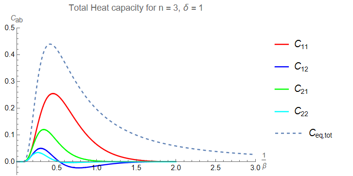
Note further that, for δ0𝛿0\delta\neq 0 and β𝛽\beta close enough to 111, c11,c12subscript𝑐11subscript𝑐12c_{11},c_{12} are positive, while c21,c22subscript𝑐21subscript𝑐22c_{21},c_{22} are negative (for δ>0𝛿0\delta>0), which is a nonequilibrium effect. However, their sum gives

c11+c12+c21+c22=ceq(1+δ24)+O(β1)subscript𝑐11subscript𝑐12subscript𝑐21subscript𝑐22subscript𝑐eq1superscript𝛿24𝑂𝛽1c_{11}+c_{12}+c_{21}+c_{22}=c_{\text{eq}}\cdot\left(1+\frac{\delta^{2}}{4}\right)+O(\beta-1) (45)

which holds for all δ𝛿\delta and is positive. Therefore, near the phase transition β=1𝛽1\beta=1 for n=0𝑛0n=0, the total heat capacity is larger than the equilibrium one and quadratic in δ𝛿\delta.

Adding g0𝑔0g\neq 0 leads to, e.g.,

c12=cabeq(1+δ2)subscript𝑐12subscriptsuperscript𝑐eq𝑎𝑏1𝛿2\displaystyle c_{12}=c^{\text{eq}}_{ab}\cdot(1+\frac{\delta}{2}) (1+δ(1+δ2)2(β1)132(13g)δ4116(13g)δ338δ2(30g2g+3(13g)2)\displaystyle\Bigg{(}1+\frac{\delta(1+\frac{\delta}{2})}{2(\beta-1)}-\frac{1}{32(1-3g)}\delta^{4}-\frac{1}{16(1-3g)}\delta^{3}-\frac{3}{8}\delta^{2}\left(\frac{30g^{2}-g+3}{(1-3g)^{2}}\right)
34δ(12g2+11g+1(13g)2))\displaystyle-\frac{3}{4}\delta\left(\frac{12g^{2}+11g+1}{(1-3g)^{2}}\right)\Bigg{)}

with a similar form for the other cabsubscript𝑐𝑎𝑏c_{ab}. As such, the critical exponent of β𝛽\beta remains α=1𝛼1\alpha=1, while the divergence at g=13𝑔13g=\frac{1}{3} takes place with a new critical exponent ν=3𝜈3\nu=3 when δ0𝛿0\delta\neq 0 (remember that cabeq(13g)1proportional-tosuperscriptsubscript𝑐𝑎𝑏eqsuperscript13𝑔1c_{ab}^{\text{eq}}\propto(\frac{1}{3}-g)^{-1}).

Finally, for the simplest case with n=1𝑛1n=1, where g=h=0𝑔0g=h=0, the heat capacities take the form

cab=cabeq(1+δFab(δ)ββc(δ)+δGab(δ))+O(ββc(δ))subscript𝑐𝑎𝑏superscriptsubscript𝑐𝑎𝑏eq1𝛿subscript𝐹𝑎𝑏𝛿𝛽subscript𝛽𝑐𝛿𝛿subscript𝐺𝑎𝑏𝛿𝑂𝛽subscript𝛽𝑐𝛿\displaystyle c_{ab}=c_{ab}^{\text{eq}}\Big{(}1+\frac{\delta\ F_{ab}(\delta)}{\beta-\beta_{c}(\delta)}+\delta\ G_{ab}(\delta)\Big{)}+O\left(\beta-\beta_{c}(\delta)\right) (46)

where Fab(δ),Gab(δ)subscript𝐹𝑎𝑏𝛿subscript𝐺𝑎𝑏𝛿F_{ab}(\delta),G_{ab}(\delta) are known for general δ𝛿\delta. The form (46) is qualitatively similar to the n=0𝑛0n=0 case, but where βcsubscript𝛽𝑐\beta_{c} becomes δ𝛿\delta-dependent. In particular, the critical exponent α=1𝛼1\alpha=1 is unchanged.

5.3 Low-temperature asymptotics

We consider two possible low-temperature limits of the heat capacity evaluated in a stable magnetization. In each case, the specific heat is either zero or decays exponentially to zero, as expected from more general grounds (extended Third Law of Thermodynamics for nonequilibrium systems); see [16].

Limit 1

We consider first the low-temperature limit β1,β2subscript𝛽1subscript𝛽2\beta_{1},\beta_{2}\to\infty, keeping the nonequilibrium driving δ=β2β1𝛿subscript𝛽2subscript𝛽1\delta=\beta_{2}-\beta_{1} (and hence a finite temperature difference) fixed. Then, the specific heats go to zero exponentially fast with rate |ψ(±1)|=±ψ(±1)superscript𝜓plus-or-minus1plus-or-minus𝜓plus-or-minus1|\psi^{\prime}(\pm 1)|=\pm\psi(\pm 1),

cab4kBβ2ψ(±1)2(1+e±δψ(±1))e2β(±ψ(±1))subscript𝑐𝑎𝑏4subscript𝑘𝐵superscript𝛽2superscript𝜓superscriptplus-or-minus121superscript𝑒plus-or-minus𝛿superscript𝜓plus-or-minus1superscript𝑒2𝛽plus-or-minussuperscript𝜓plus-or-minus1c_{ab}\approx 4k_{B}\frac{\beta^{2}\psi^{\prime}(\pm 1)^{2}}{(1+e^{\pm\delta\ \psi^{\prime}(\pm 1)})}e^{-2\beta\big{(}\pm\psi^{\prime}(\pm 1)\big{)}} (47)

We first find the stationary magnetisation under the limit in question. Following (27), msubscript𝑚m_{*} satisfies

((β+δ2)n(βδ2)n)((β+δ2)n+(βδ2)n)tanhδ2ψ(m)=sinhβψ(m)mcoshβψ(m)msinhβψ(m)coshβψ(m)superscript𝛽𝛿2𝑛superscript𝛽𝛿2𝑛superscript𝛽𝛿2𝑛superscript𝛽𝛿2𝑛𝛿2superscript𝜓subscript𝑚𝛽superscript𝜓subscript𝑚subscript𝑚𝛽superscript𝜓subscript𝑚subscript𝑚𝛽superscript𝜓subscript𝑚𝛽superscript𝜓subscript𝑚\frac{\left((\beta+\frac{\delta}{2})^{n}-(\beta-\frac{\delta}{2})^{n}\right)}{\left((\beta+\frac{\delta}{2})^{n}+(\beta-\frac{\delta}{2})^{n}\right)}\tanh{\frac{\delta}{2}\psi^{\prime}(m_{*})}=-\frac{\sinh{\beta\psi^{\prime}(m_{*})}-m_{*}\cosh{\beta\psi^{\prime}(m_{*})}}{m_{*}\sinh{\beta\psi^{\prime}(m_{*})}-\cosh{\beta\psi^{\prime}(m_{*})}} (48)

For all n𝑛n, the left hand side of (48) reduces to

((β+δ2)n(βδ2)n)((β+δ2)n+(βδ2)n)0 when β at fixed δ superscript𝛽𝛿2𝑛superscript𝛽𝛿2𝑛superscript𝛽𝛿2𝑛superscript𝛽𝛿2𝑛0 when β at fixed δ \frac{\left((\beta+\frac{\delta}{2})^{n}-(\beta-\frac{\delta}{2})^{n}\right)}{\left((\beta+\frac{\delta}{2})^{n}+(\beta-\frac{\delta}{2})^{n}\right)}\downarrow 0\text{ when $\beta\uparrow\infty$ at fixed $\delta$ }

Hence, for β𝛽\beta\uparrow\infty, the stationary magnetization solves

m=tanhβψ(m)subscript𝑚𝛽superscript𝜓subscript𝑚m_{*}=\tanh{\beta\psi^{\prime}(m_{*})} (49)

which is independent of n,δ𝑛𝛿n,\delta and agrees with the n=0𝑛0n=0 case, (31). For h=00h=0, m=0subscript𝑚0m_{*}=0 is always a solution to (49), but it becomes unstable for β𝛽\beta large enough. Indeed, m=0subscript𝑚0m_{*}=0 changes stability when H(0)=0superscript𝐻00H^{\prime}(0)=0, i.e., at β=βc(n,δ)𝛽subscript𝛽𝑐𝑛𝛿\beta=\beta_{c}(n,\delta) where

2(βc(n,δ)1)[(βc(n,δ)δ/2)n\displaystyle 2(\beta_{c}(n,\delta)-1)\Biggl{[}(\beta_{c}(n,\delta)-\delta/2)^{-n} +(βc(n,δ)+δ/2)n]\displaystyle+(\beta_{c}(n,\delta)+\delta/2)^{-n}\Biggr{]} (50)
+[(βc(n,δ)δ/2)n+(βc(n,δ)+δ/2)n]δ=0delimited-[]superscriptsubscript𝛽𝑐𝑛𝛿𝛿2𝑛superscriptsubscript𝛽𝑐𝑛𝛿𝛿2𝑛𝛿0\displaystyle+\Biggl{[}-(\beta_{c}(n,\delta)-\delta/2)^{-n}+(\beta_{c}(n,\delta)+\delta/2)^{-n}\Biggr{]}\delta=0

In the limit considered, βc(n,δ)subscript𝛽𝑐𝑛𝛿\beta_{c}(n,\delta) is constant since n,δ𝑛𝛿n,\delta are fixed quantities. As such, for β>βc(n,δ)𝛽subscript𝛽𝑐𝑛𝛿\beta>\beta_{c}(n,\delta), the zero magnetisation m=0subscript𝑚0m_{*}=0 is unstable. Focus thus on the nonzero solutions m0subscript𝑚0m_{*}\neq 0 of (49) for β𝛽\beta\uparrow\infty. Using tanhx=±(12e2x+o(e2x))𝑥plus-or-minus12superscript𝑒minus-or-plus2𝑥𝑜superscript𝑒2𝑥\tanh{x}=\pm(1-2e^{\mp 2x}+o(e^{-2x})) for x±𝑥plus-or-minusx\uparrow\pm\infty leads to

m=±(12e2βψ(m))subscript𝑚plus-or-minus12superscript𝑒minus-or-plus2𝛽superscript𝜓subscript𝑚m_{*}=\pm(1-2e^{\mp 2\beta\psi^{\prime}(m_{*})}) (51)

where the upper sign is for m>0subscript𝑚0m_{*}>0 and the other for m<0subscript𝑚0m_{*}<0. Taking m=±(1ε)subscript𝑚plus-or-minus1𝜀m_{*}=\pm(1-\varepsilon) with ε1much-less-than𝜀1\varepsilon\ll 1 in (51) and expanding to first order in ε𝜀\varepsilon, results in

ε=2e2βψ(±1)1+4e2βψ(1)βψ′′(±1)2e2βψ(±1)𝜀2superscript𝑒minus-or-plus2𝛽superscript𝜓plus-or-minus114superscript𝑒minus-or-plus2𝛽superscript𝜓1𝛽superscript𝜓′′plus-or-minus12superscript𝑒minus-or-plus2𝛽superscript𝜓plus-or-minus1\varepsilon=\frac{2e^{\mp 2\beta\psi^{\prime}(\pm 1)}}{1+4e^{\mp 2\beta\psi^{\prime}(1)}\beta\psi^{\prime\prime}(\pm 1)}\approx 2e^{\mp 2\beta\psi^{\prime}(\pm 1)}

Thus, m±(12e2βψ(±1))subscript𝑚plus-or-minus12superscript𝑒minus-or-plus2𝛽superscript𝜓plus-or-minus1m_{*}\approx\pm(1-2e^{\mp 2\beta\psi^{\prime}(\pm 1)}) for β𝛽\beta\uparrow\infty, and

mβ=±4ψ(±1)e2βψ(±1)subscript𝑚𝛽plus-or-minus4superscript𝜓plus-or-minus1superscript𝑒minus-or-plus2𝛽superscript𝜓plus-or-minus1\frac{\partial m_{*}}{\partial\beta}=\pm 4\psi^{\prime}(\pm 1)e^{\mp 2\beta\psi^{\prime}(\pm 1)} (52)

which decreases exponentially. Furthermore,

JkBβj2ψ′′(m)Ha(m)+ψ(m)Ha(m)H(m)±kBβ2ψ(±1)J(1+e±δψ(±1))𝐽subscript𝑘𝐵superscriptsubscript𝛽𝑗2superscript𝜓′′subscript𝑚subscript𝐻𝑎subscript𝑚superscript𝜓subscript𝑚subscriptsuperscript𝐻𝑎subscript𝑚superscript𝐻subscript𝑚plus-or-minussubscript𝑘𝐵superscript𝛽2superscript𝜓plus-or-minus1𝐽1superscript𝑒plus-or-minus𝛿superscript𝜓plus-or-minus1Jk_{B}\beta_{j}^{2}\frac{\psi^{\prime\prime}(m_{*})H_{a}(m_{*})+\psi^{\prime}(m_{*})H^{\prime}_{a}(m_{*})}{H^{\prime}(m_{*})}\approx\pm k_{B}\frac{\beta^{2}\psi^{\prime}(\pm 1)}{J(1+e^{\pm\delta\ \psi^{\prime}(\pm 1)})} (53)

Combining (52) and (53) in (39), we obtain (47)

cab4kBβ2ψ(±1)2(1+e±δψ(±1))e2β(±ψ(±1))subscript𝑐𝑎𝑏4subscript𝑘𝐵superscript𝛽2superscript𝜓superscriptplus-or-minus121superscript𝑒plus-or-minus𝛿superscript𝜓plus-or-minus1superscript𝑒2𝛽plus-or-minussuperscript𝜓plus-or-minus1c_{ab}\approx 4k_{B}\frac{\beta^{2}\psi^{\prime}(\pm 1)^{2}}{(1+e^{\pm\delta\ \psi^{\prime}(\pm 1)})}e^{-2\beta\big{(}\pm\psi^{\prime}(\pm 1)\big{)}}

which decreases exponentially to 00 with rate ±ψ(±1)=|ψ(±1)|plus-or-minussuperscript𝜓plus-or-minus1superscript𝜓plus-or-minus1\pm\psi^{\prime}(\pm 1)=|\psi^{\prime}(\pm 1)| and is independent of n𝑛n.

Limit 2

Another interesting limits occurs by taking β2subscript𝛽2\beta_{2}\to\infty, keeping β1subscript𝛽1\beta_{1} fixed, i.e., β,δ𝛽𝛿\beta,\delta\uparrow\infty keeping β1=1J(βδ2)subscript𝛽11𝐽𝛽𝛿2\beta_{1}=\frac{1}{J}(\beta-\frac{\delta}{2}) fixed, i.e., we only lower the temperature of the second bath. Then, the heat capacities c11,c12subscript𝑐11subscript𝑐12c_{11},c_{12} and c22subscript𝑐22c_{22} vanish, while c21subscript𝑐21c_{21} reduces to the equilibrium result (41) at temperature β1subscript𝛽1\beta_{1},

c21kBJψ(m)β12mβ1c11=c22=c12=0formulae-sequencesubscript𝑐21subscript𝑘𝐵𝐽superscript𝜓subscript𝑚superscriptsubscript𝛽12subscript𝑚subscript𝛽1subscript𝑐11subscript𝑐22subscript𝑐120c_{21}\approx k_{B}J\psi^{\prime}(m_{*})\beta_{1}^{2}\frac{\partial m_{*}}{\partial\beta_{1}}\qquad c_{11}=c_{22}=c_{12}=0 (54)

To show, we note that analyzing (50) in the limit δ𝛿\delta\to\infty leads to

βc(n,δ)1+δ2proportional-tosubscript𝛽𝑐𝑛𝛿1𝛿2\beta_{c}(n,\delta)\propto 1+\frac{\delta}{2}

Since m=0subscript𝑚0m_{*}=0 is stable for β<βc(n,δ)𝛽subscript𝛽𝑐𝑛𝛿\beta<\beta_{c}(n,\delta), it follows that for Jβ11𝐽subscript𝛽11J\beta_{1}\leq 1, cab=0subscript𝑐𝑎𝑏0c_{ab}=0. In the other case Jβ1>1𝐽subscript𝛽11J\beta_{1}>1, the stable magnetisation is ferromagnetic m0subscript𝑚0m_{*}\neq 0 and satisfies

1m1±m=e2Jβ1ψ(m)minus-or-plus1subscript𝑚plus-or-minus1subscript𝑚superscript𝑒minus-or-plus2𝐽subscript𝛽1superscript𝜓subscript𝑚\frac{1\mp m_{*}}{1\pm m_{*}}=e^{\mp 2J\beta_{1}\psi^{\prime}(m_{*})} (55)

where we get the upper sign for m>0subscript𝑚0m_{*}>0 and the lower sign for m<0subscript𝑚0m_{*}<0. Equation (55) is obtained from (27) in the limit β,δ𝛽𝛿\beta,\delta\uparrow\infty. As a consequence,

mβ2subscript𝑚subscript𝛽2\displaystyle\frac{\partial m_{*}}{\partial\beta_{2}} =\displaystyle= 00\displaystyle 0
mβ1subscript𝑚subscript𝛽1\displaystyle\frac{\partial m_{*}}{\partial\beta_{1}} =\displaystyle= ±e2Jβ1ψ(m)Jψ(m)1(1±m)2e2Jβ1ψ(m)β1Jψ′′(m)=±Jψ(m)(1m2)1(1m2)β1Jψ′′(m)plus-or-minussuperscript𝑒minus-or-plus2𝐽subscript𝛽1superscript𝜓subscript𝑚𝐽superscript𝜓subscript𝑚1superscriptplus-or-minus1subscript𝑚2superscript𝑒minus-or-plus2𝐽subscript𝛽1superscript𝜓subscript𝑚subscript𝛽1𝐽superscript𝜓′′subscript𝑚plus-or-minus𝐽superscript𝜓subscript𝑚1superscriptsubscript𝑚211superscriptsubscript𝑚2subscript𝛽1𝐽superscript𝜓′′subscript𝑚\displaystyle\frac{\pm e^{\mp 2J\beta_{1}\psi^{\prime}(m_{*})}J\psi^{\prime}(m_{*})}{\frac{1}{(1\pm m_{*})^{2}}-e^{\mp 2J\beta_{1}\psi^{\prime}(m_{*})}\beta_{1}J\psi^{\prime\prime}(m_{*})}=\frac{\pm J\psi^{\prime}(m_{*})(1-m_{*}^{2})}{1-(1-m_{*}^{2})\beta_{1}J\psi^{\prime\prime}(m_{*})} (56)

Furthermore, for (39) in the limit β2subscript𝛽2\beta_{2}\uparrow\infty,

limβ2JkBβ12ψ′′(m)H2(m)+ψ(m)H2(m)H1(m)+H2(m)=±kBJψ(m)β12subscriptsubscript𝛽2𝐽subscript𝑘𝐵superscriptsubscript𝛽12superscript𝜓′′subscript𝑚subscript𝐻2subscript𝑚superscript𝜓subscript𝑚subscriptsuperscript𝐻2subscript𝑚subscriptsuperscript𝐻1subscript𝑚subscriptsuperscript𝐻2subscript𝑚plus-or-minussubscript𝑘𝐵𝐽superscript𝜓subscript𝑚superscriptsubscript𝛽12\displaystyle\lim_{\beta_{2}\to\infty}Jk_{B}\beta_{1}^{2}\frac{\psi^{\prime\prime}(m_{*})H_{2}(m_{*})+\psi^{\prime}(m_{*})H^{\prime}_{2}(m_{*})}{H^{\prime}_{1}(m_{*})+H^{\prime}_{2}(m_{*})}=\pm k_{B}J\psi^{\prime}(m_{*})\beta_{1}^{2} (57)
limβ2JkBβ12ψ′′(m)H1(m)+ψ(m)H1(m)H1(m)+H2(m)=0subscriptsubscript𝛽2𝐽subscript𝑘𝐵superscriptsubscript𝛽12superscript𝜓′′subscript𝑚subscript𝐻1subscript𝑚superscript𝜓subscript𝑚subscriptsuperscript𝐻1subscript𝑚subscriptsuperscript𝐻1subscript𝑚subscriptsuperscript𝐻2subscript𝑚0\displaystyle\lim_{\beta_{2}\to\infty}Jk_{B}\beta_{1}^{2}\frac{\psi^{\prime\prime}(m_{*})H_{1}(m_{*})+\psi^{\prime}(m_{*})H^{\prime}_{1}(m_{*})}{H^{\prime}_{1}(m_{*})+H^{\prime}_{2}(m_{*})}=0 (58)

By combining (5.3) and (57)-(58) in (38), we conclude that for Jβ1>1𝐽subscript𝛽11J\beta_{1}>1 and β2subscript𝛽2\beta_{2}\uparrow\infty,

c21kBJψ(m)β12mβ1c11=c22=c12=0formulae-sequencesubscript𝑐21subscript𝑘𝐵𝐽superscript𝜓subscript𝑚superscriptsubscript𝛽12subscript𝑚subscript𝛽1subscript𝑐11subscript𝑐22subscript𝑐120c_{21}\approx k_{B}J\psi^{\prime}(m_{*})\beta_{1}^{2}\frac{\partial m_{*}}{\partial\beta_{1}}\qquad c_{11}=c_{22}=c_{12}=0 (59)

which is (54). Therefore, all the excess heat by changing β1subscript𝛽1\beta_{1} is produced in the second heat bath. That is physically clear as any heat will immediately flow to the zero-temperature β2subscript𝛽2\beta_{2}\to\infty bath. Furthermore, that c12,c22=0subscript𝑐12subscript𝑐220c_{12},c_{22}=0 is a manifestation of the Third Law of Thermodynamics.
The form of c21subscript𝑐21c_{21} in (54) agrees with the equilibrium result at inverse temperature β1subscript𝛽1\beta_{1} as in (41), but msubscript𝑚m_{*} does not satisfy the equilibrium equation (31). Furthermore, from (5.3), it follows that c21subscript𝑐21c_{21} goes exponentially to zero with rate |ψ(±1)|superscript𝜓plus-or-minus1|\psi^{\prime}(\pm 1)| in case the additional limit β1subscript𝛽1\beta_{1}\uparrow\infty is taken.

6 Computation of the specific heat matrix

6.1 Macroscopic Poisson equation

To derive the formula (38) for the specific heats cabsubscript𝑐𝑎𝑏c_{ab}, we need to understand the thermodynamic behaviour of the (extensive) quasipotential (13), solution of

LNVa(σ)=Nja,NsPa,N(σ)superscript𝐿𝑁subscript𝑉𝑎𝜎𝑁superscriptsubscript𝑗𝑎𝑁𝑠subscript𝑃𝑎𝑁𝜎L^{N}V_{a}\,(\sigma)=Nj_{a,N}^{s}-P_{a,N}(\sigma) (60)

in the limit N𝑁N\uparrow\infty. We do that in the next paragraph by expanding both the left and right-hand side of equation (60) to order O(1N)𝑂1𝑁O\left(\frac{1}{N}\right). We already put here the limiting Poisson equation,

SN𝒱a′′(m)+(H(m)+H~(m)Nψ′′(m))𝒱a(m)=NJFa(m)JGa(m)+O(1N)𝑆𝑁superscriptsubscript𝒱𝑎′′𝑚𝐻𝑚~𝐻𝑚𝑁superscript𝜓′′𝑚superscriptsubscript𝒱𝑎𝑚𝑁𝐽subscript𝐹𝑎𝑚𝐽subscript𝐺𝑎𝑚𝑂1𝑁\frac{S}{N}\mathcal{V}_{a}^{\prime\prime}(m)+\left(H(m)+\frac{\tilde{H}(m)}{N}\psi^{\prime\prime}(m)\right)\mathcal{V}_{a}^{\prime}(m)=-NJF_{a}(m)-JG_{a}(m)+O\left(\frac{1}{N}\right) (61)

where the smooth function 𝒱a(m),m[1,+1]subscript𝒱𝑎𝑚𝑚11{\mathcal{V}}_{a}(m),m\in[-1,+1] is called the macroscopic quasipotential. Similar to the heat capacity, the macroscopic quasipotential is extensive, i.e. 𝒱(m)Nproportional-to𝒱𝑚𝑁\mathcal{V}(m)\propto N, which makes sure that the neglected terms are order O(1N)𝑂1𝑁O\left(\frac{1}{N}\right). The functions Fa,Gasubscript𝐹𝑎subscript𝐺𝑎F_{a},G_{a} are given below in (67)-(68) while S,H~𝑆~𝐻S,\tilde{H} are given in (69).
Note that the stationary dissipation ja,Nssuperscriptsubscript𝑗𝑎𝑁𝑠j_{a,N}^{s} in (60) depends on a choice of stationary magnetization msubscript𝑚m_{*}. The calculation must indeed be done in a stable phase of the phase diagram, characterized by some msubscript𝑚m_{*} which is a differentiable function of the βasubscript𝛽𝑎\beta_{a}. We fix therefore a stationary and stable magnetization msubscript𝑚m_{*}, i.e., a solution of H(m)=0,H(m)<0formulae-sequence𝐻subscript𝑚0superscript𝐻subscript𝑚0H(m_{*})=0,H^{\prime}(m_{*})<0.

Expansion of (60):

We start by writing out the right-hand side of (60). The heat (10) sent to the thermal bath at inverse temperature βasubscript𝛽𝑎\beta_{a} when flipping the k𝑘k-th spin equals

qa,N(σ,k)=1βalogca(σ,k)ca(σk,k)=2J[ψ(mN(σ))σk1Nψ′′(mN(σ))+O(1N2)]subscript𝑞𝑎𝑁𝜎𝑘1subscript𝛽𝑎subscript𝑐𝑎𝜎𝑘subscript𝑐𝑎superscript𝜎𝑘𝑘2𝐽delimited-[]superscript𝜓superscript𝑚𝑁𝜎subscript𝜎𝑘1𝑁superscript𝜓′′superscript𝑚𝑁𝜎𝑂1superscript𝑁2q_{a,N}(\sigma,k)=\frac{1}{\beta_{a}}\log\frac{c_{a}(\sigma,k)}{c_{a}(\sigma^{k},k)}=-2J\left[\psi^{\prime}(m^{N}(\sigma))\sigma_{k}-\frac{1}{N}\psi^{\prime\prime}(m^{N}(\sigma))+O\left(\frac{1}{N^{2}}\right)\right]

where we use the asymptotics (23). When the configuration is σ𝜎\sigma, the instantaneously expected heat flux (power) (11) to the heat bath a𝑎a at inverse temperature βasubscript𝛽𝑎\beta_{a} is, therefore,

Pa,Nsubscript𝑃𝑎𝑁\displaystyle P_{a,N} =kca(σ,k)qa,N(σ,k)=NJψ(mN(σ))Ha(mN(σ))absentsubscript𝑘subscript𝑐𝑎𝜎𝑘subscript𝑞𝑎𝑁𝜎𝑘𝑁𝐽superscript𝜓superscript𝑚𝑁𝜎subscript𝐻𝑎superscript𝑚𝑁𝜎\displaystyle=\sum_{k}c_{a}(\sigma,k)\,q_{a,N}(\sigma,k)=N\,J\psi^{\prime}(m^{N}(\sigma))\,H_{a}(m^{N}(\sigma)) (62)
+J[Sa(mN(σ))+βaJψ(mN(σ))Ha(mN(σ))]ψ′′(mN(σ))+O(1N)𝐽delimited-[]subscript𝑆𝑎superscript𝑚𝑁𝜎subscript𝛽𝑎𝐽superscript𝜓superscript𝑚𝑁𝜎subscript𝐻𝑎superscript𝑚𝑁𝜎superscript𝜓′′superscript𝑚𝑁𝜎𝑂1𝑁\displaystyle+J\left[S_{a}(m^{N}(\sigma))+\beta_{a}J\psi^{\prime}(m^{N}(\sigma))H_{a}(m^{N}(\sigma))\right]\psi^{\prime\prime}(m^{N}(\sigma))+O\left(\frac{1}{N}\right)

with Hasubscript𝐻𝑎H_{a} defined in (20) and

Sa(m):=2ν(Jβa)n[cosh(Jβaψ(m))msinh(Jβaψ(m))]assignsubscript𝑆𝑎𝑚2𝜈superscript𝐽subscript𝛽𝑎𝑛delimited-[]𝐽subscript𝛽𝑎superscript𝜓𝑚𝑚𝐽subscript𝛽𝑎superscript𝜓𝑚\displaystyle S_{a}(m):=\frac{2\nu}{(J\beta_{a})^{n}}\left[\cosh(J\beta_{a}\psi^{\prime}(m))-m\,\sinh(J\beta_{a}\psi^{\prime}(m))\right] (63)

In the steady regime with stationary magnetization msubscript𝑚m_{*}, the heat current to the a𝑎a-th reservoir, per number of spins, is (12) and becomes

ja,Ns(m)superscriptsubscript𝑗𝑎𝑁𝑠subscript𝑚\displaystyle j_{a,N}^{s}(m_{*}) =1NPa,NNsabsent1𝑁superscriptsubscriptdelimited-⟨⟩subscript𝑃𝑎𝑁𝑁𝑠\displaystyle=\frac{1}{N}\langle P_{a,N}\rangle_{N}^{s} (64)
=Jψ(m)Ha(m)+ψ′′(m)N(Sa(m)+βaJψ(m)Ha(m))+O(1N2)absent𝐽superscript𝜓subscript𝑚subscript𝐻𝑎subscript𝑚superscript𝜓′′subscript𝑚𝑁subscript𝑆𝑎subscript𝑚subscript𝛽𝑎𝐽superscript𝜓subscript𝑚subscript𝐻𝑎subscript𝑚𝑂1superscript𝑁2\displaystyle=J\ \psi^{\prime}(m_{*})\,H_{a}(m_{*})+\frac{\psi^{\prime\prime}(m_{*})}{N}\Big{(}S_{a}(m_{*})+\beta_{a}J\psi^{\prime}(m_{*})H_{a}(m_{*})\Big{)}+O\left(\frac{1}{N^{2}}\right)

As a consequence, using (62) and (64), when mN(σ)msuperscript𝑚𝑁𝜎𝑚m^{N}(\sigma)\to m, the right-hand side of the macroscopic Poisson equation (60) becomes

Nja,Ns(m)Pa,N=NJFa(m)JGa(m)+O(1N)𝑁superscriptsubscript𝑗𝑎𝑁𝑠subscript𝑚subscript𝑃𝑎𝑁𝑁𝐽subscript𝐹𝑎𝑚𝐽subscript𝐺𝑎𝑚𝑂1𝑁\displaystyle Nj_{a,N}^{s}(m_{*})-P_{a,N}=-NJF_{a}(m)-JG_{a}(m)+O\left(\frac{1}{N}\right) (65)

where

Fa(m)subscript𝐹𝑎𝑚\displaystyle F_{a}(m) =ψ(m)Ha(m)ψ(mN)Ha(mN)absentsuperscript𝜓𝑚subscript𝐻𝑎𝑚superscript𝜓superscriptsubscript𝑚𝑁subscript𝐻𝑎superscriptsubscript𝑚𝑁\displaystyle=\psi^{\prime}(m)\,H_{a}(m)-\psi^{\prime}(m_{*}^{N})\,H_{a}(m_{*}^{N}) (66)
Ga(m)subscript𝐺𝑎𝑚\displaystyle G_{a}(m) =Sa(m)ψ′′(m)Sa(mN)ψ′′(mN)absentsubscript𝑆𝑎𝑚superscript𝜓′′𝑚subscript𝑆𝑎superscriptsubscript𝑚𝑁superscript𝜓′′superscriptsubscript𝑚𝑁\displaystyle=S_{a}(m)\psi^{\prime\prime}(m)-S_{a}(m_{*}^{N})\psi^{\prime\prime}(m_{*}^{N}) (67)
+βaJ(ψ(m)ψ′′(m)Ha(m)ψ(mN)ψ′′(mN)Ha(mN))subscript𝛽𝑎𝐽superscript𝜓𝑚superscript𝜓′′𝑚subscript𝐻𝑎𝑚superscript𝜓superscriptsubscript𝑚𝑁superscript𝜓′′superscriptsubscript𝑚𝑁subscript𝐻𝑎superscriptsubscript𝑚𝑁\displaystyle+\beta_{a}J\Big{(}\psi^{\prime}(m)\psi^{\prime\prime}(m)H_{a}(m)-\psi^{\prime}(m_{*}^{N})\psi^{\prime\prime}(m_{*}^{N})H_{a}(m_{*}^{N})\Big{)} (68)

Next comes the left-hand side of the Poisson equation (60). Since all the terms on the right-hand side depend on mN(σ)superscript𝑚𝑁𝜎m^{N}(\sigma), we use mN(σ)msuperscript𝑚𝑁𝜎𝑚m^{N}(\sigma)\longrightarrow m and make the Ansatz Va=Va(mN(σ))subscript𝑉𝑎subscript𝑉𝑎superscript𝑚𝑁𝜎V_{a}=V_{a}(m^{N}(\sigma)). Now, for an arbitrary smooth function f𝑓f of m[1,1]𝑚11m\in[-1,1],

LNf(mN(σ))=k=1Nc(σ,k)[f(mN(σ)2Nσk)f(mN(σ))]superscript𝐿𝑁𝑓superscript𝑚𝑁𝜎superscriptsubscript𝑘1𝑁𝑐𝜎𝑘delimited-[]𝑓superscript𝑚𝑁𝜎2𝑁subscript𝜎𝑘𝑓superscript𝑚𝑁𝜎\displaystyle L^{N}f\big{(}m^{N}(\sigma)\big{)}=\sum_{k=1}^{N}c(\sigma,k)\Big{[}f\big{(}m^{N}(\sigma)-\frac{2}{N}\sigma_{k}\big{)}-f\big{(}m^{N}(\sigma)\big{)}\Big{]}

where mN(σk)=mN(σ)2Nσksuperscript𝑚𝑁superscript𝜎𝑘superscript𝑚𝑁𝜎2𝑁subscript𝜎𝑘m^{N}(\sigma^{k})=m^{N}(\sigma)-\frac{2}{N}\sigma_{k}. Using identities like

f(mN(σ)2Nσk)f(mN(σ))𝑓superscript𝑚𝑁𝜎2𝑁subscript𝜎𝑘𝑓superscript𝑚𝑁𝜎\displaystyle f\big{(}m^{N}(\sigma)-\frac{2}{N}\sigma_{k}\big{)}-f\big{(}m^{N}(\sigma)\big{)} =\displaystyle= 2Nf(mN(σ))σk+2N2f′′(mN(σ))+O(1N3)2𝑁superscript𝑓superscript𝑚𝑁𝜎subscript𝜎𝑘2superscript𝑁2superscript𝑓′′superscript𝑚𝑁𝜎𝑂1superscript𝑁3\displaystyle-\frac{2}{N}f^{\prime}\big{(}m^{N}(\sigma)\big{)}\sigma_{k}+\frac{2}{N^{2}}f^{\prime\prime}\big{(}m^{N}(\sigma)\big{)}+O\left(\frac{1}{N^{3}}\right)
k=1NeJβaσkψ(mN(σ))σksuperscriptsubscript𝑘1𝑁superscript𝑒𝐽subscript𝛽𝑎subscript𝜎𝑘superscript𝜓superscript𝑚𝑁𝜎subscript𝜎𝑘\displaystyle\color[rgb]{0,0,0}\definecolor[named]{pgfstrokecolor}{rgb}{0,0,0}\pgfsys@color@gray@stroke{0}\pgfsys@color@gray@fill{0}\sum_{k=1}^{N}e^{-J\beta_{a}\sigma_{k}\psi^{\prime}\big{(}m^{N}(\sigma)\big{)}}\sigma_{k} =\displaystyle= N(Jβa)n2νHa(mN(σ))𝑁superscript𝐽subscript𝛽𝑎𝑛2𝜈subscript𝐻𝑎superscript𝑚𝑁𝜎\displaystyle-\frac{N(J\beta_{a})^{n}}{2\nu}H_{a}\big{(}m^{N}(\sigma)\big{)}
k=1NeJβaσkψ(mN(σ))superscriptsubscript𝑘1𝑁superscript𝑒𝐽subscript𝛽𝑎subscript𝜎𝑘superscript𝜓superscript𝑚𝑁𝜎\displaystyle\sum_{k=1}^{N}e^{-J\beta_{a}\sigma_{k}\psi^{\prime}\big{(}m^{N}(\sigma)\big{)}} =\displaystyle= N(Jβa)n2νSa(mN(σ))𝑁superscript𝐽subscript𝛽𝑎𝑛2𝜈subscript𝑆𝑎superscript𝑚𝑁𝜎\displaystyle\frac{N(J\beta_{a})^{n}}{2\nu}S_{a}\big{(}m^{N}(\sigma)\big{)}

we obtain for mN(σ)msuperscript𝑚𝑁𝜎𝑚m^{N}(\sigma)\to m that

LNf(mN(σ))=H(m)f(m)+1N(S(m)f′′(m)+H~(m)f(m)ψ′′(m))+O(1N2)superscript𝐿𝑁𝑓superscript𝑚𝑁𝜎𝐻𝑚superscript𝑓𝑚1𝑁𝑆𝑚superscript𝑓′′𝑚~𝐻𝑚superscript𝑓𝑚superscript𝜓′′𝑚𝑂1superscript𝑁2L^{N}f\big{(}m^{N}(\sigma)\big{)}=H(m)f^{\prime}(m)+\frac{1}{N}\Big{(}S(m)f^{\prime\prime}(m)+\tilde{H}(m)f^{\prime}(m)\psi^{\prime\prime}(m)\Big{)}+O\left(\frac{1}{N^{2}}\right)

where

S(m):=S1(m)+S2(m)H~(m):=J(β1H1(m)+β2H2(m))formulae-sequenceassign𝑆𝑚subscript𝑆1𝑚subscript𝑆2𝑚assign~𝐻𝑚𝐽subscript𝛽1subscript𝐻1𝑚subscript𝛽2subscript𝐻2𝑚S(m):=S_{1}(m)+S_{2}(m)\qquad\tilde{H}(m):=J\big{(}\beta_{1}H_{1}(m)+\beta_{2}H_{2}(m)\big{)} (69)

In the limit N𝑁N\uparrow\infty, the solution to equation (60) is a smooth function 𝒱a(m),m[1,+1]subscript𝒱𝑎𝑚𝑚11{\mathcal{V}}_{a}(m),m\in[-1,+1] (macroscopic quasipotential). Combined with the source term (65), we see that it verifies the macroscopic Poisson equation (61).

6.2 Macroscopic quasipotential

Defining the derivative Wa=𝒱asubscript𝑊𝑎superscriptsubscript𝒱𝑎W_{a}=\mathcal{V}_{a}^{\prime}, the solutions of (61) for Wasubscript𝑊𝑎W_{a} and 𝒱asubscript𝒱𝑎\mathcal{V}_{a} become

Wa(m)subscript𝑊𝑎𝑚\displaystyle W_{a}(m) =em~mNS(H+H~Nψ′′)dmabsentsuperscript𝑒superscriptsubscript~𝑚𝑚𝑁𝑆𝐻~𝐻𝑁superscript𝜓′′dsuperscript𝑚\displaystyle=e^{\int_{\tilde{m}}^{m}-\frac{N}{S}(H+\frac{\tilde{H}}{N}\psi^{\prime\prime})\ \textrm{d}m^{\prime}} (70)
[Wa(m~)NJm~mdm′′(em~m′′NS(H+H~Nψ′′)dm)1S(Fa+GaN)]delimited-[]subscript𝑊𝑎~𝑚𝑁𝐽superscriptsubscript~𝑚𝑚dsuperscript𝑚′′superscript𝑒superscriptsubscript~𝑚superscript𝑚′′𝑁𝑆𝐻~𝐻𝑁superscript𝜓′′dsuperscript𝑚1𝑆subscript𝐹𝑎subscript𝐺𝑎𝑁\displaystyle\Big{[}W_{a}(\tilde{m})-NJ\int_{\tilde{m}}^{m}\textrm{d}m^{\prime\prime}\ \left(e^{\int_{\tilde{m}}^{m^{\prime\prime}}\ \frac{N}{S}(H+\frac{\tilde{H}}{N}\psi^{\prime\prime})\textrm{d}m^{\prime}}\right)\frac{1}{S}\left(F_{a}+\frac{G_{a}}{N}\right)\Big{]}
𝒱a(m)subscript𝒱𝑎𝑚\displaystyle\mathcal{V}_{a}(m) =mmWa(m)dmabsentsuperscriptsubscriptsubscript𝑚𝑚subscript𝑊𝑎superscript𝑚dsuperscript𝑚\displaystyle=\int_{m_{*}}^{m}W_{a}(m^{\prime})\ \textrm{d}m^{\prime} (71)

where m~~𝑚\tilde{m} is an integration constant and we used (14). The solution (71) is well-defined because the integrands are continuously differentiable everywhere and S(m)0𝑆𝑚0S(m)\neq 0 for m[1,1]𝑚11m\in[-1,1]. To see this, remark that, using (63), S(m)=0𝑆𝑚0S(m)=0 would imply

m=(Jβ2)ncoshJβ1ψ(m)+(Jβ1)ncoshJβ2ψ(m)(Jβ2)nsinhJβ1ψ(m)+(Jβ1)nsinhJβ1ψ(m)>1𝑚superscript𝐽subscript𝛽2𝑛𝐽subscript𝛽1superscript𝜓subscript𝑚superscript𝐽subscript𝛽1𝑛𝐽subscript𝛽2superscript𝜓subscript𝑚superscript𝐽subscript𝛽2𝑛𝐽subscript𝛽1superscript𝜓subscript𝑚superscript𝐽subscript𝛽1𝑛𝐽subscript𝛽1superscript𝜓subscript𝑚1m=\frac{(J\beta_{2})^{n}\cosh{J\beta_{1}\psi^{\prime}(m_{*})}+(J\beta_{1})^{n}\cosh{J\beta_{2}\psi^{\prime}(m_{*})}}{(J\beta_{2})^{n}\sinh{J\beta_{1}\psi^{\prime}(m_{*})}+(J\beta_{1})^{n}\sinh{J\beta_{1}\psi^{\prime}(m_{*})}}>1 (72)

which is not in the integration domains [1,1]11[-1,1]. Since, furthermore, S(0)>0𝑆00S(0)>0, it holds that S(m)>0𝑆𝑚0S(m)>0 for all m[1,1]𝑚11m\in[-1,1].

It follows from requiring that the exponential factor be bounded for all m𝑚m when N𝑁N\uparrow\infty that m~{0,+1,1}~𝑚011\tilde{m}\in\{0,+1,-1\}. Indeed, the thermodynamic limit is well-defined when the integral

m~m1S(H+H~Nψ′′)dmsuperscriptsubscript~𝑚𝑚1𝑆𝐻~𝐻𝑁superscript𝜓′′dsuperscript𝑚\int_{\tilde{m}}^{m}\frac{1}{S}\left(H+\frac{\tilde{H}}{N}\psi^{\prime\prime}\right)\ \textrm{d}m^{\prime} (73)

is positive for all m𝑚m. In the limit N𝑁N\uparrow\infty, the sign of (73) is determined fully by the sign of the integral over H𝐻H, from which it follows that, depending on the chosen temperature pair, m~{1,0,1}~𝑚101\tilde{m}\in\{-1,0,1\}. For example, when m=0subscript𝑚0m_{*}=0 is unstable (H(0)>0superscript𝐻00H^{\prime}(0)>0), then the integral will be positive for all m𝑚m when m~=0~𝑚0\tilde{m}=0. Otherwise, when m=0subscript𝑚0m_{*}=0 is stable, the behaviour of the integrand changes, and one must take m~=±1~𝑚plus-or-minus1\tilde{m}=\pm 1.

6.3 Specific heat calculation

To find the heat capacity (38), the βbsubscript𝛽𝑏\beta_{b}-derivative of the macroscopic quasipotential (71) need to be taken, which requires a careful analysis to lead us to the conclusion (39).

We start by taking βbsubscript𝛽𝑏\beta_{b} derivatives of the macroscopic quasipotential (71), which gives

𝒱aβb=Wa(m)mβb+mmWaβbdmsubscript𝒱𝑎subscript𝛽𝑏subscript𝑊𝑎subscript𝑚subscript𝑚subscript𝛽𝑏superscriptsubscriptsubscript𝑚𝑚subscript𝑊𝑎subscript𝛽𝑏dsuperscript𝑚\frac{\partial\mathcal{V}_{a}}{\partial\beta_{b}}=W_{a}(m_{*})\ \frac{\partial m_{*}}{\partial\beta_{b}}+\int_{m_{*}}^{m}\frac{\partial W_{a}}{\partial\beta_{b}}\ \textrm{d}m^{\prime}

with

Waβb=em~mNS(H+H~Nψ′′)dm{Wa(m~)βbWa(m~)m~mdmβb[NS(H+H~Nψ′′)]\displaystyle\frac{\partial W_{a}}{\partial\beta_{b}}=e^{\int_{\tilde{m}}^{m}-\frac{N}{S}(H+\frac{\tilde{H}}{N}\psi^{\prime\prime})\ \textrm{d}m^{\prime}}\Big{\{}\frac{\partial W_{a}(\tilde{m})}{\partial\beta_{b}}-W_{a}(\tilde{m})\int_{\tilde{m}}^{m}\textrm{d}m^{\prime}\ \frac{\partial}{\partial\beta_{b}}\Big{[}\frac{N}{S}(H+\frac{\tilde{H}}{N}\psi^{\prime\prime})\Big{]}
+NJm~mdmβb[NS(H+H~Nψ′′)]m~mdm′′[em~m′′NS(H+H~Nψ′′)dm1S(Fa+GaN)]𝑁𝐽superscriptsubscript~𝑚𝑚dsuperscript𝑚subscript𝛽𝑏delimited-[]𝑁𝑆𝐻~𝐻𝑁superscript𝜓′′superscriptsubscript~𝑚𝑚dsuperscript𝑚′′delimited-[]superscript𝑒superscriptsubscript~𝑚superscript𝑚′′𝑁𝑆𝐻~𝐻𝑁superscript𝜓′′dsuperscript𝑚1𝑆subscript𝐹𝑎subscript𝐺𝑎𝑁\displaystyle+NJ\int_{\tilde{m}}^{m}\textrm{d}m^{\prime}\ \frac{\partial}{\partial\beta_{b}}\Big{[}\frac{N}{S}(H+\frac{\tilde{H}}{N}\psi^{\prime\prime})\Big{]}\cdot\int_{\tilde{m}}^{m}\textrm{d}m^{\prime\prime}\ \Big{[}e^{\int_{\tilde{m}}^{m^{\prime\prime}}\frac{N}{S}(H+\frac{\tilde{H}}{N}\psi^{\prime\prime})\ \textrm{d}m^{\prime}}\frac{1}{S}\left(F_{a}+\frac{G_{a}}{N}\right)\Big{]}
NJm~mdm′′βb[em~m′′NS(H+H~Nψ′′)dm1S(Fa+GaN)]}\displaystyle-NJ\int_{\tilde{m}}^{m}\textrm{d}m^{\prime\prime}\ \frac{\partial}{\partial\beta_{b}}\Big{[}e^{\int_{\tilde{m}}^{m^{\prime\prime}}\frac{N}{S}(H+\frac{\tilde{H}}{N}\psi^{\prime\prime})\ \textrm{d}m^{\prime}}\frac{1}{S}\left(F_{a}+\frac{G_{a}}{N}\right)\Big{]}\Big{\}}

This derivative is analytic everywhere on its integration domain such that in the limit mm𝑚subscript𝑚m\to m_{*}, the integral mmWaβbdmsuperscriptsubscriptsubscript𝑚𝑚subscript𝑊𝑎subscript𝛽𝑏dsuperscript𝑚\int_{m_{*}}^{m}\frac{\partial W_{a}}{\partial\beta_{b}}\ \textrm{d}m^{\prime} does not contribute. Therefore,

𝒱aβb(m)=Wa(m)mβbsubscript𝒱𝑎subscript𝛽𝑏subscript𝑚subscript𝑊𝑎subscript𝑚subscript𝑚subscript𝛽𝑏\frac{\partial\mathcal{V}_{a}}{\partial\beta_{b}}(m_{*})=W_{a}(m_{*})\frac{\partial m_{*}}{\partial\beta_{b}} (74)

Note further that in the limit N𝑁N\uparrow\infty, (70) and (71) reduce to

wa(m)=limNWa(m)N=Jψ(m)Ha(m)ψ(m)Ha(m)H(m)for mm~subscript𝑤𝑎𝑚subscript𝑁subscript𝑊𝑎𝑚𝑁𝐽superscript𝜓𝑚subscript𝐻𝑎𝑚superscript𝜓subscript𝑚subscript𝐻𝑎subscript𝑚𝐻𝑚for mm~\displaystyle w_{a}(m)=\lim_{N\uparrow\infty}\frac{W_{a}(m)}{N}=-J\frac{\psi^{\prime}(m)H_{a}(m)-\psi^{\prime}(m_{*})H_{a}(m_{*})}{H(m)}\ \text{for $m\neq\tilde{m}$}
va(m)=limN𝒱a(m)N=Jmmψ(m)Ha(m)ψ(m)Ha(m)H(m)subscript𝑣𝑎𝑚subscript𝑁subscript𝒱𝑎𝑚𝑁𝐽superscriptsubscriptsubscript𝑚𝑚superscript𝜓𝑚subscript𝐻𝑎𝑚superscript𝜓subscript𝑚subscript𝐻𝑎subscript𝑚𝐻𝑚\displaystyle v_{a}(m)=\lim_{N\uparrow\infty}\frac{\mathcal{V}_{a}(m)}{N}=-J\int_{m_{*}}^{m}\frac{\psi^{\prime}(m)H_{a}(m)-\psi^{\prime}(m_{*})H_{a}(m_{*})}{H(m)}

and

wa(m)=limmmJψ(m)Ha(m)ψ(m)Ha(m)H(m)subscript𝑤𝑎subscript𝑚subscript𝑚subscript𝑚𝐽superscript𝜓𝑚subscript𝐻𝑎𝑚superscript𝜓subscript𝑚subscript𝐻𝑎subscript𝑚𝐻𝑚\displaystyle w_{a}(m_{*})=\lim_{m\to m_{*}}-J\frac{\psi^{\prime}(m)H_{a}(m)-\psi^{\prime}(m_{*})H_{a}(m_{*})}{H(m)}
=Jψ′′(m)Ha(m)+ψ(m)Ha(m)H(m)for mm~absent𝐽superscript𝜓′′subscript𝑚subscript𝐻𝑎subscript𝑚superscript𝜓subscript𝑚superscriptsubscript𝐻𝑎subscript𝑚superscript𝐻subscript𝑚for mm~\displaystyle=-J\frac{\psi^{\prime\prime}(m_{*})H_{a}(m_{*})+\psi^{\prime}(m_{*})H_{a}^{\prime}(m_{*})}{H^{\prime}(m_{*})}\ \text{for $m_{*}\neq\tilde{m}$} (75)

Taking N𝑁N\uparrow\infty and using (6.3), we conclude that

limN1N𝒱aβb=Jmβbψ′′(m)Ha(m)+ψ(m)Ha(m)H(m)subscript𝑁1𝑁subscript𝒱𝑎subscript𝛽𝑏𝐽subscript𝑚subscript𝛽𝑏superscript𝜓′′subscript𝑚subscript𝐻𝑎subscript𝑚superscript𝜓subscript𝑚subscriptsuperscript𝐻𝑎subscript𝑚superscript𝐻subscript𝑚\lim_{N}\frac{1}{N}\frac{\partial\mathcal{V}_{a}}{\partial\beta_{b}}=J\frac{\partial m_{*}}{\partial\beta_{b}}\frac{\psi^{\prime\prime}(m_{*})H_{a}(m_{*})+\psi^{\prime}(m_{*})H^{\prime}_{a}(m_{*})}{H^{\prime}(m_{*})} (76)

Note that applying (6.3) only holds for mm~{1,0,1}subscript𝑚~𝑚101m_{*}\neq\tilde{m}\in\{-1,0,1\}, but since Wa(m)subscript𝑊𝑎subscript𝑚W_{a}(m_{*}) is multiplied by mβbsubscript𝑚subscript𝛽𝑏\frac{\partial m_{*}}{\partial\beta_{b}} in (74), which is zero for m{1,0,1}subscript𝑚101m_{*}\in\{-1,0,1\}, the last expression is valid for all msubscript𝑚m_{*}. From (76), the main formula for the specific heat (39) follows

cab(m)subscript𝑐𝑎𝑏subscript𝑚\displaystyle c_{ab}(m_{*}) =limN1NkBβb2𝒱aβb(m,σ)Nsabsentsubscript𝑁1𝑁subscript𝑘𝐵superscriptsubscript𝛽𝑏2subscriptsuperscriptdelimited-⟨⟩subscript𝒱𝑎subscript𝛽𝑏subscript𝑚𝜎𝑠𝑁\displaystyle=\lim_{N}\frac{1}{N}k_{B}\beta_{b}^{2}\Big{\langle}\frac{\partial\mathcal{V}_{a}}{\partial\beta_{b}}(m_{*},\sigma)\Big{\rangle}^{s}_{N}
=kBβb2Jmβbψ′′(m)Ha(m)+ψ(m)Ha(m)H(m)absentsubscript𝑘𝐵superscriptsubscript𝛽𝑏2𝐽subscript𝑚subscript𝛽𝑏superscript𝜓′′subscript𝑚subscript𝐻𝑎subscript𝑚superscript𝜓subscript𝑚subscriptsuperscript𝐻𝑎subscript𝑚superscript𝐻subscript𝑚\displaystyle=k_{B}\beta_{b}^{2}J\frac{\partial m_{*}}{\partial\beta_{b}}\frac{\psi^{\prime\prime}(m_{*})H_{a}(m_{*})+\psi^{\prime}(m_{*})H^{\prime}_{a}(m_{*})}{H^{\prime}(m_{*})} (77)

We finally observe that, by the symmetry of the reservoirs,

c11c22=c12c21subscript𝑐11subscript𝑐22subscript𝑐12subscript𝑐21c_{11}c_{22}=c_{12}c_{21}

implying that the determinant of the specific heat matrix vanishes. One can indeed not always reconstruct the temperature changes from observing the excess heat.

7 Summary and outlook

The Curie-Weiss model is turned into a nonequilibrium spin model by randomly switching between thermal baths. The phase diagrams change with the degree of nonequilibrium, also depending significantly on the temperature dependence of the time-symmetric part in the spin-flip rates. Most notably, new regions of stability may arise for otherwise unstable phases. Furthermore, the critical temperature moves with the nonequilibrium amplitude.
The nonequilibrium specific heat is obtained in the thermodynamic limit N𝑁N\uparrow\infty following the excess heat formalism. In contrast with the standard Curie-Weiss model, where the specific heat shows a jump at the critical temperature, under the two-temperature driving, it diverges at the (also new) phase transitions with critical exponent α=1𝛼1\alpha=1. The low-temperature asymptotics satisfies an extended Nernst postulate, and the specific heat vanishes exponentially fast at absolute zero.

We believe that the two-temperature Curie-Weiss model is the first to combine a systematic study of the nonequilibrium phase diagram with an analysis of thermal response in terms of heat capacity. Other response functions can certainly be studied as well. On the other hand, our model is slightly artificial and does not directly lead to a more general Landau-type view on the influence of nonequilibrium aspects on phase transitions [2]. As a matter of fact, and in contrast with equilibrium, different versions of mean-field modelling may exist, possibly giving quite different results.
Extensions of our work indeed include a Landau field theory approach, taking a finite switching rate r𝑟r between reservoirs as in (4) and including kinetically-different thermal baths. They make the subjects of future work.

Acknowledgment: The two-temperature Curie-Weiss model of the present paper was first proposed by Karel Netočný to study the nonequilibrium phase diagram. We are grateful for his suggestion.
Furthermore, the authors thank the reviewers for their thoughtful comments and useful suggestions.

Data Availability: Data sharing is not applicable to this article as no data sets were generated or analyzed during the current study.

Conflict of interest The authors have no relevant financial or non-financial interests to disclose.

Appendix A Example: N=2𝑁2N=2

When the system consists of two spins, the magnetization becomes mN=2=σ1+σ22{1,0,1}superscript𝑚𝑁2subscript𝜎1subscript𝜎22101m^{N=2}=\frac{\sigma_{1}+\sigma_{2}}{2}\in\{-1,0,1\}, and energy E(σ)=Jg1+σ1σ22{0,Jg}𝐸𝜎subscript𝐽𝑔1subscript𝜎1subscript𝜎220subscript𝐽𝑔E(\sigma)=-J_{g}\frac{1+\sigma_{1}\sigma_{2}}{2}\in\{0,-J_{g}\}, where Jg=J(1+g2)subscript𝐽𝑔𝐽1𝑔2J_{g}=J\big{(}1+\frac{g}{2}\big{)}. Therefore, the process reduces to a two-level switch where g𝑔g only affects the energy difference.

First, the heat fluxes (11), Pa,N=2(σ)subscript𝑃𝑎𝑁2𝜎P_{a,N=2}(\sigma) become

Pa,N(1,1)=Pa,N(1,1)subscript𝑃𝑎𝑁11subscript𝑃𝑎𝑁11\displaystyle P_{a,N}(1,1)=P_{a,N}(-1,-1) =2Jgν(Jgβa)neβaJg2,absent2subscript𝐽𝑔𝜈superscriptsubscript𝐽𝑔subscript𝛽𝑎𝑛superscript𝑒subscript𝛽𝑎subscript𝐽𝑔2\displaystyle=-\frac{2J_{g}\nu}{(J_{g}\beta_{a})^{n}}e^{-\beta_{a}\frac{J_{g}}{2}},
Pa,N(1,1)=Pa,N(1,1)subscript𝑃𝑎𝑁11subscript𝑃𝑎𝑁11\displaystyle P_{a,N}(1,-1)=P_{a,N}(-1,1) =2Jgν(Jgβa)neβaJg2absent2subscript𝐽𝑔𝜈superscriptsubscript𝐽𝑔subscript𝛽𝑎𝑛superscript𝑒subscript𝛽𝑎subscript𝐽𝑔2\displaystyle=\frac{2J_{g}\nu}{(J_{g}\beta_{a})^{n}}e^{\beta_{a}\frac{J_{g}}{2}}

The quasipotential Va(N=2)superscriptsubscript𝑉𝑎𝑁2V_{a}^{(N=2)} in (13) takes the form Va(N=2)=(Va1,Va2,Va2,Va1)superscriptsubscript𝑉𝑎𝑁2subscript𝑉𝑎1subscript𝑉𝑎2subscript𝑉𝑎2subscript𝑉𝑎1V_{a}^{(N=2)}=(V_{a1},V_{a2},V_{a2},V_{a1}) with

Va1subscript𝑉𝑎1\displaystyle V_{a1} =vabe12(2βa+βb)Jg(eβaJg2βan+eβbJg2βbn)absentsubscript𝑣𝑎𝑏superscript𝑒122subscript𝛽𝑎subscript𝛽𝑏subscript𝐽𝑔superscript𝑒subscript𝛽𝑎subscript𝐽𝑔2superscriptsubscript𝛽𝑎𝑛superscript𝑒subscript𝛽𝑏subscript𝐽𝑔2superscriptsubscript𝛽𝑏𝑛\displaystyle=-v_{ab}\ e^{-\frac{1}{2}\left(2\beta_{a}+\beta_{b}\right)J_{g}}\left(e^{\frac{\beta_{a}J_{g}}{2}}\beta_{a}^{n}+e^{\frac{\beta_{b}J_{g}}{2}}\beta_{b}^{n}\right)
Va2subscript𝑉𝑎2\displaystyle V_{a2} =vabeβaJg2(eβbJg2βan+eβaJg2βbn)absentsubscript𝑣𝑎𝑏superscript𝑒subscript𝛽𝑎subscript𝐽𝑔2superscript𝑒subscript𝛽𝑏subscript𝐽𝑔2superscriptsubscript𝛽𝑎𝑛superscript𝑒subscript𝛽𝑎subscript𝐽𝑔2superscriptsubscript𝛽𝑏𝑛\displaystyle=v_{ab}\ e^{-\frac{\beta_{a}J_{g}}{2}}\left(e^{\frac{\beta_{b}J_{g}}{2}}\beta_{a}^{n}+e^{\frac{\beta_{a}J_{g}}{2}}\beta_{b}^{n}\right)
vabsubscript𝑣𝑎𝑏\displaystyle v_{ab} =Jg(eβaJg+1)βbn(2β1ncosh(β2Jg2)+2β2ncosh(β1Jg2))2absentsubscript𝐽𝑔superscript𝑒subscript𝛽𝑎subscript𝐽𝑔1superscriptsubscript𝛽𝑏𝑛superscript2superscriptsubscript𝛽1𝑛subscript𝛽2subscript𝐽𝑔22superscriptsubscript𝛽2𝑛subscript𝛽1subscript𝐽𝑔22\displaystyle=J_{g}\left(e^{\beta_{a}J_{g}}+1\right)\beta_{b}^{n}\left(2\beta_{1}^{n}\cosh\left(\frac{\beta_{2}J_{g}}{2}\right)+2\beta_{2}^{n}\cosh\left(\frac{\beta_{1}J_{g}}{2}\right)\right)^{-2}

where ab𝑎𝑏a\neq b. That, from (15), leads to the heat capacities,

Caa(N=2)=kBC~abβaβb2n(Jgβaβbn+JgcoshJg2(βaβb)2nβansinhJg2(βaβb))superscriptsubscript𝐶𝑎𝑎𝑁2subscript𝑘𝐵subscript~𝐶𝑎𝑏subscript𝛽𝑎superscriptsubscript𝛽𝑏2𝑛subscript𝐽𝑔subscript𝛽𝑎superscriptsubscript𝛽𝑏𝑛subscript𝐽𝑔subscript𝐽𝑔2subscript𝛽𝑎subscript𝛽𝑏2𝑛superscriptsubscript𝛽𝑎𝑛subscript𝐽𝑔2subscript𝛽𝑎subscript𝛽𝑏\displaystyle C_{aa}^{(N=2)}=k_{B}\ \tilde{C}_{ab}\ \beta_{a}\ \beta_{b}^{2n}\left(J_{g}\beta_{a}\beta_{b}^{n}+J_{g}\cosh{\frac{J_{g}}{2}(\beta_{a}-\beta_{b})}-2\ n\ \beta_{a}^{n}\sinh{\frac{J_{g}}{2}(\beta_{a}-\beta_{b})}\right)
Cab(N=2)=kBC~abβanβbn+1(Jgβanβb+Jgβbn+1coshJg2(βaβb)+2nβbnsinhJg2(βaβb))superscriptsubscript𝐶𝑎𝑏𝑁2subscript𝑘𝐵subscript~𝐶𝑎𝑏superscriptsubscript𝛽𝑎𝑛superscriptsubscript𝛽𝑏𝑛1subscript𝐽𝑔superscriptsubscript𝛽𝑎𝑛subscript𝛽𝑏subscript𝐽𝑔superscriptsubscript𝛽𝑏𝑛1subscript𝐽𝑔2subscript𝛽𝑎subscript𝛽𝑏2𝑛superscriptsubscript𝛽𝑏𝑛subscript𝐽𝑔2subscript𝛽𝑎subscript𝛽𝑏\displaystyle C_{ab}^{(N=2)}=k_{B}\ \tilde{C}_{ab}\ \beta_{a}^{n}\ \beta_{b}^{n+1}\left(J_{g}\beta_{a}^{n}\beta_{b}+J_{g}\beta_{b}^{n+1}\cosh{\frac{J_{g}}{2}(\beta_{a}-\beta_{b})}+2\ n\ \beta_{b}^{n}\sinh{\frac{J_{g}}{2}(\beta_{a}-\beta_{b})}\right)
C~ab=Jg4coshJβa2(β1ncosh(β2Jg2)+β2ncosh(β1Jg2))3subscript~𝐶𝑎𝑏subscript𝐽𝑔4𝐽subscript𝛽𝑎2superscriptsuperscriptsubscript𝛽1𝑛subscript𝛽2subscript𝐽𝑔2superscriptsubscript𝛽2𝑛subscript𝛽1subscript𝐽𝑔23\displaystyle\tilde{C}_{ab}=\frac{J_{g}}{4}\cosh{\frac{J\beta_{a}}{2}}\left(\beta_{1}^{n}\cosh\left(\frac{\beta_{2}J_{g}}{2}\right)+\beta_{2}^{n}\cosh\left(\frac{\beta_{1}J_{g}}{2}\right)\right)^{-3}

where again ab𝑎𝑏a\neq b. In equilibrium β2=β1subscript𝛽2subscript𝛽1\beta_{2}=\beta_{1}, all of them reduce to

Ceq,ab(N=2)=kBβ12Jg2eβ1Jg4(eβ1Jg+1)2superscriptsubscript𝐶eq,𝑎𝑏𝑁2subscript𝑘𝐵superscriptsubscript𝛽12superscriptsubscript𝐽𝑔2superscript𝑒subscript𝛽1subscript𝐽𝑔4superscriptsuperscript𝑒subscript𝛽1subscript𝐽𝑔12C_{\text{eq,}ab}^{(N=2)}=k_{B}\frac{\beta_{1}^{2}J_{g}^{2}e^{\beta_{1}J_{g}}}{4\left(e^{\beta_{1}J_{g}}+1\right)^{2}}

which is a quarter of the total equilibrium heat capacity Ceq,totsubscript𝐶eq,totC_{\text{eq,tot}} for a two-level system [36].
The heat capacities are plotted in Fig. 9, where some are seen to obtain negative values, here for n=3𝑛3n=3. As discussed in [37], this happens due to a negative correlation between the quasipotential Va(N)superscriptsubscript𝑉𝑎𝑁V_{a}^{(N)} and the change in stationary distribution ρssuperscript𝜌𝑠\rho^{s}.

Refer to caption
Figure 9: Heat capacities vs 1β=(Jgβ1+β22)11𝛽superscriptsubscript𝐽𝑔subscript𝛽1subscript𝛽221\frac{1}{\beta}=\big{(}J_{g}\frac{\beta_{1}+\beta_{2}}{2}\big{)}^{-1} for n=3𝑛3n=3 and δ=Jg(β2β1)=1𝛿subscript𝐽𝑔subscript𝛽2subscript𝛽11\delta=J_{g}\big{(}\beta_{2}-\beta_{1}\big{)}=1. The graphs stop at β=δ2𝛽𝛿2\beta=\frac{\delta}{2} where β1=0subscript𝛽10\beta_{1}=0. We plot the total equilibrium result Ceq, totsubscript𝐶eq, totC_{\text{eq, tot}} with a dashed line. (Made using Mathematica version 13.1.0.0 [35].)

References