Fast Optimal Transport through Sliced Wasserstein Generalized Geodesics

Guillaume Mahey
INSA Rouen-Université Bretagne Sud
LITIS - IRISA
guillaume.mahey@insa-rouen.fr
&Laetitia Chapel
Université Bretagne Sud
IRISA
laetitia.chapel@univ-ubs.fr
&Gilles Gasso
INSA Rouen
LITIS
gilles.gasso@insa-rouen.fr
&Clément Bonet
Université Bretagne Sud
LMBA
clément.bonet@univ-ubs.fr
&Nicolas Courty
Université Bretagne Sud
IRISA
nicolas.courty@univ-ubs.fr
Abstract

Wasserstein distance (WD) and the associated optimal transport plan have proven useful in many applications where probability measures are at stake. In this paper, we propose a new proxy for the squared WD, coined min-SWGG, which relies on the transport map induced by an optimal one-dimensional projection of the two input distributions. We draw connections between min-SWGG and Wasserstein generalized geodesics with a pivot measure supported on a line. We notably provide a new closed form of the Wasserstein distance in the particular case where one of the distributions is supported on a line, allowing us to derive a fast computational scheme that is amenable to gradient descent optimization. We show that min-SWGG is an upper bound of WD and that it has a complexity similar to that of Sliced-Wasserstein, with the additional feature of providing an associated transport plan. We also investigate some theoretical properties such as metricity, weak convergence, computational and topological properties. Empirical evidences support the benefits of min-SWGG in various contexts, from gradient flows, shape matching and image colorization, among others.

1 Introduction

Gaspard Monge, in his seminal work on Optimal Transport (OT) [42], studied the following problem: how to move with minimum cost the probability mass of a source measure to a target one, for a given transfer cost function? At the heart of OT is the optimal map that describes the optimal displacement as the Monge problem can be reformulated as an assignment problem. It has been relaxed by [33] by finding a plan that describes the amount of mass moving from the source to the target. Beyond this optimal plan, an interest of OT is that it defines a distance between probability measures: the Wasserstein distance (WD).

Recently, OT has been successfully employed in a wide range of machine learning applications, in which the Wasserstein distance is estimated from the data, such as supervised learning [30], natural language processing [38] or generative modelling [5]. Its capacity to provide meaningful distances between empirical distributions is at the core of distance-based algorithms such as kernel-based methods [60] or k𝑘k-nearest neighbors [6]. The optimal transport plan has also been used successfully in many applications where a matching between empirical samples is sought such as color transfer [55], domain adaptation [19] and positive-unlabeled learning [15].

Solving the OT problem is computationally intensive; the most common algorithmic tools to solve the discrete OT problem are borrowed from combinatorial optimization and linear programming, leading to a cubic complexity with the number of samples that prevents its use in large scale applications [53]. To reduce the computation burden, regularizing the OT problem with e.g. an entropic term has led to solvers with a quadratic complexity [23]. Other methods based on the existence of a closed form of OT have also been devised to efficiently compute a proxy for WD, as outlined below.

Projections-based OT. The Sliced-Wasserstein distance (SWD) [56, 10] leverages 1D-projections of distributions to provide a lower approximation of the Wasserstein distance, relying on the closed form of OT for 1D probability distributions. Computation of SWD leads to a linearithmic time complexity. While SWD averages WDs computed over several 1D projections, max-SWD [24] keeps only the most informative projection. These frameworks provide efficient algorithms that can handle millions of samples and have similar topological properties as WD [45]. Other works restrain SWD and max-SWD to projections onto low dimensional subspaces [52, 40] to provide more robust estimation of those OT metrics. Although effective as proxies for WD, those methods do not provide a transport plan in the original space dsuperscript𝑑\mathbb{R}^{d}. To overcome this limitation, [44] aims to compute transport plans in a subspace which are extrapolated to the original space.

Pivot measure-based OT. Other research works rely on a pivot, yet intermediate measure. They decompose the OT metric into Wasserstein distances between each input measure and the considered pivot measure. They exhibit better properties such as statistical sample complexity or computational efficiency [29, 65]. Even though the OT problems are split, they are still expensive when dealing with large sample size distributions, notably when only two distributions are involved.

Contributions. We introduce a new proxy for the squared WD that exploits the principles of aforementioned approximations of OT metric. The original idea is to rely on projections and one-dimensional assignment of the projected distributions to compute the new proxy. The approach is well-grounded as it hinges on the notion of Wasserstein generalized geodesics [4] with pivot measure supported on a line. The main features of the method are as: i) its computational complexity is on par with SW, ii) it provides an optimal transport plan through the 1D assignment problem, iii) it acts as an upper bound of WD, and iv) is amenable to optimization to find the optimal pivot measure. As an additional contribution, we establish a closed form of the WD when an input measure is supported on a line.

Outline. Section 2 presents some background of OT. Section 3 formulates our new WD proxy, provides some of its topological properties and a numerical computation scheme. Section 4 builds upon the concept of Wasserstein generalized geodesics to reformulate our OT metric approximation as the Sliced Wasserstein Generalized Geodesics (SWGG) along its optimal variant coined min-SWGG. This reformulation allows deriving additional topological properties and an optimization scheme. Finally, Section 5 provides experimental evaluations.

Notations. Let ,\langle\cdot,\cdot\rangle be the Euclidean inner product on dsuperscript𝑑\mathbb{R}^{d} and let 𝕊d1={𝒖d s.t. 𝒖2=1}superscript𝕊𝑑1conditional-set𝒖superscript𝑑 s.t. evaluated-at𝒖21\mathbb{S}^{d-1}=\{\boldsymbol{u}\in\mathbb{R}^{d}\text{ s.t. }\|\boldsymbol{u}\|_{2}=1\}, the unit sphere. We denote 𝒫(d)𝒫superscript𝑑\mathcal{P}(\mathbb{R}^{d}) the set of probability measures on dsuperscript𝑑\mathbb{R}^{d} endowed with the σlimit-from𝜎\sigma-algebra of Borel set and 𝒫2(d)𝒫(d)subscript𝒫2superscript𝑑𝒫superscript𝑑\mathcal{P}_{2}(\mathbb{R}^{d})\subset\mathcal{P}(\mathbb{R}^{d}) those with finite second-order moment i.e. 𝒫2(d)={μ𝒫(d) s.t. d𝒙22dμ(𝒙)<}subscript𝒫2superscript𝑑conditional-set𝜇𝒫superscript𝑑 s.t. subscriptsuperscript𝑑evaluated-at𝒙22𝑑𝜇𝒙\mathcal{P}_{2}(\mathbb{R}^{d})=\{\mu\in\mathcal{P}(\mathbb{R}^{d})\text{ s.t. }\int_{\mathbb{R}^{d}}\|\boldsymbol{x}\|^{2}_{2}d\mu(\boldsymbol{x})<\infty\}. Let 𝒫2n(d)subscriptsuperscript𝒫𝑛2superscript𝑑\mathcal{P}^{n}_{2}(\mathbb{R}^{d}) be the subspace of 𝒫2(d)subscript𝒫2superscript𝑑\mathcal{P}_{2}(\mathbb{R}^{d}) defined by empirical measures with n𝑛n-atoms and uniform masses. For any measurable function f:dd:𝑓superscript𝑑superscript𝑑f:\mathbb{R}^{d}\to\mathbb{R}^{d}, we denote f#subscript𝑓#f_{\#} its push forward, namely for μ𝒫2(d)𝜇subscript𝒫2superscript𝑑\mu\in\mathcal{P}_{2}(\mathbb{R}^{d}) and for any measurable set Ad𝐴superscript𝑑A\in\mathbb{R}^{d}, f#μ(A)=μ(f1(A))subscript𝑓#𝜇𝐴𝜇superscript𝑓1𝐴f_{\#}\mu(A)=\mu(f^{-1}(A)), with f1(A)={𝒙d s.t. f(𝒙)A}superscript𝑓1𝐴𝒙superscript𝑑 s.t. 𝑓𝒙𝐴f^{-1}(A)=\{\boldsymbol{x}\in\mathbb{R}^{d}\text{ s.t. }f(\boldsymbol{x})\in A\}.

2 Background on Optimal Transport

Definition 2.1 (Wasserstein distance).

The squared WD [63] between μ1,μ2𝒫2(d)subscript𝜇1subscript𝜇2subscript𝒫2superscript𝑑\mu_{1},\mu_{2}\in\mathcal{P}_{2}(\mathbb{R}^{d}) is defined as:

W22(μ1,μ2)=definfπΠ(μ1,μ2)d×d𝒙𝒚22𝑑π(𝒙,𝒚)superscriptdefsubscriptsuperscript𝑊22subscript𝜇1subscript𝜇2subscriptinfimum𝜋Πsubscript𝜇1subscript𝜇2subscriptsuperscript𝑑superscript𝑑superscriptsubscriptnorm𝒙𝒚22differential-d𝜋𝒙𝒚W^{2}_{2}(\mu_{1},\mu_{2})\stackrel{{\scriptstyle\text{def}}}{{\,\,=\,}}\inf_{\pi\in\Pi(\mu_{1},\mu_{2})}\int_{\mathbb{R}^{d}\times\mathbb{R}^{d}}\|\boldsymbol{x}-\boldsymbol{y}\|_{2}^{2}d\pi(\boldsymbol{x},\boldsymbol{y}) (1)

with Π(μ1,μ2)={π𝒫2(d×d)\Pi(\mu_{1},\mu_{2})=\{\pi\in\mathcal{P}_{2}(\mathbb{R}^{d}\times\mathbb{R}^{d}) s.t. π(A×d)=μ1(A)𝜋𝐴superscript𝑑subscript𝜇1𝐴\pi(A\times\mathbb{R}^{d})=\mu_{1}(A) and π(d×A)=μ2(A)𝜋superscript𝑑𝐴subscript𝜇2𝐴\pi(\mathbb{R}^{d}\times A)=\mu_{2}(A), Afor-all𝐴\forall A measurable set of d}\mathbb{R}^{d}\}.

The argmin\arg\min of Eq. (1) is referred to as the optimal transport plan. Denoted πsuperscript𝜋\pi^{*}, it expresses how to move the probability mass from μ1subscript𝜇1\mu_{1} to μ2subscript𝜇2\mu_{2} with minimum cost. In some cases, πsuperscript𝜋\pi^{*} is of the form (Id,T)#μ1subscript𝐼𝑑𝑇#subscript𝜇1(Id,T)_{\#}\mu_{1} for a measurable map T:dd:𝑇superscript𝑑superscript𝑑T:\mathbb{R}^{d}\to\mathbb{R}^{d}, i.e. there is no mass splitting during the transport. This map is called a Monge map and is denoted Tμ1μ2superscript𝑇subscript𝜇1subscript𝜇2T^{\mu_{1}\to\mu_{2}} (or shortly T12superscript𝑇12T^{1\to 2}). Thus, one has W22(μ1,μ2)=infTs.t.T#μ1=μ2d𝒙T(𝒙)22𝑑μ1(𝒙)subscriptsuperscript𝑊22subscript𝜇1subscript𝜇2subscriptinfimum𝑇s.t.subscript𝑇#subscript𝜇1subscript𝜇2subscriptsuperscript𝑑subscriptsuperscriptnorm𝒙𝑇𝒙22differential-dsubscript𝜇1𝒙W^{2}_{2}(\mu_{1},\mu_{2})=\inf_{T\;\text{s.t.}\;T_{\#}\mu_{1}=\mu_{2}}\int_{\mathbb{R}^{d}}\|\boldsymbol{x}-T(\boldsymbol{x})\|^{2}_{2}d\mu_{1}(\boldsymbol{x}). This occurs, for instance, when μ1subscript𝜇1\mu_{1} has a density w.r.t. the Lebesgue measure [12] or when μ1subscript𝜇1\mu_{1} and μ2subscript𝜇2\mu_{2} are in 𝒫2n(d)subscriptsuperscript𝒫𝑛2superscript𝑑\mathcal{P}^{n}_{2}(\mathbb{R}^{d}) [58].

Endowed with the WD, the space 𝒫2(d)subscript𝒫2superscript𝑑\mathcal{P}_{2}(\mathbb{R}^{d}) is a geodesic space. Indeed, since there exists a Monge map T12superscript𝑇12T^{1\to 2} between μ1subscript𝜇1\mu_{1} and μ2subscript𝜇2\mu_{2}, one can define a geodesic curve μ12:[0,1]𝒫2(d):superscript𝜇1201subscript𝒫2superscript𝑑\mu^{1\to 2}:[0,1]\to\mathcal{P}_{2}(\mathbb{R}^{d}) [31] as:

t[0,1],μ12(t)=def(tT12+(1t)Id)#μ1formulae-sequencefor-all𝑡01superscriptdefsuperscript𝜇12𝑡subscript𝑡superscript𝑇121𝑡𝐼𝑑#subscript𝜇1\forall t\in[0,1],\ \mu^{1\to 2}(t)\stackrel{{\scriptstyle\text{def}}}{{\,\,=\,}}(tT^{1\to 2}+(1-t)Id)_{\#}\mu_{1} (2)

which represents the shortest path w.r.t. Wasserstein distance in 𝒫2(d)subscript𝒫2superscript𝑑\mathcal{P}_{2}(\mathbb{R}^{d}) between μ1subscript𝜇1\mu_{1} and μ2subscript𝜇2\mu_{2}. The Wasserstein mean between μ1subscript𝜇1\mu_{1} and μ2subscript𝜇2\mu_{2} corresponds to t=0.5𝑡0.5t=0.5 and we simply write μ12superscript𝜇12\mu^{1\to 2}.

This notion of geodesic allows the study of the curvature of the Wasserstein space [1]. Indeed, the Wasserstein space is of positive curvature [51], i.e. it respects the following inequality:

W22(μ1,μ2)2W22(μ1,ν)+2W22(ν,μ2)4W22(μ12,ν)subscriptsuperscript𝑊22subscript𝜇1subscript𝜇22subscriptsuperscript𝑊22subscript𝜇1𝜈2subscriptsuperscript𝑊22𝜈subscript𝜇24subscriptsuperscript𝑊22superscript𝜇12𝜈W^{2}_{2}(\mu_{1},\mu_{2})\geq 2W^{2}_{2}(\mu_{1},\nu)+2W^{2}_{2}(\nu,\mu_{2})-4W^{2}_{2}(\mu^{1\to 2},\nu) (3)

for all pivot measures ν𝒫2(d)𝜈subscript𝒫2superscript𝑑\nu\in\mathcal{P}_{2}(\mathbb{R}^{d}).

Solving and approximating Optimal Transport.

The Wasserstein distance between empirical measures μ1,μ2subscript𝜇1subscript𝜇2\mu_{1},\mu_{2} with n𝑛n-atoms can be computed in 𝒪(n3logn)𝒪superscript𝑛3𝑛\mathcal{O}(n^{3}\log n), preventing from the use of OT for large scale applications [11]. Several algorithms have been proposed to lower this complexity, for example the Sinkhorn algorithm [23] that provides an approximation in near 𝒪(n2)𝒪superscript𝑛2\mathcal{O}(n^{2}) complexity [2].

Notably, when μ1=1ni=1nδxisubscript𝜇11𝑛superscriptsubscript𝑖1𝑛subscript𝛿subscript𝑥𝑖\mu_{1}=\frac{1}{n}\sum_{i=1}^{n}\delta_{x_{i}} and μ2=1ni=1nδyisubscript𝜇21𝑛superscriptsubscript𝑖1𝑛subscript𝛿subscript𝑦𝑖\mu_{2}=\frac{1}{n}\sum_{i=1}^{n}\delta_{y_{i}} are 1D distributions, computing the WD can be done by matching the sorted empirical samples, leading to an overall complexity of 𝒪(nlogn)𝒪𝑛𝑛\mathcal{O}(n\log n). More precisely, let σ𝜎\sigma and τ𝜏\tau two permutation operators s.t. xσ(1)xσ(2)xσ(n)subscript𝑥𝜎1subscript𝑥𝜎2subscript𝑥𝜎𝑛x_{\sigma(1)}\leq x_{\sigma(2)}\leq...\leq x_{\sigma(n)} and yτ(1)yτ(2)yτ(n)subscript𝑦𝜏1subscript𝑦𝜏2subscript𝑦𝜏𝑛y_{\tau(1)}\leq y_{\tau(2)}\leq...\leq y_{\tau(n)}. Then, the 1D Wasserstein distance is given by:

W22(μ1,μ2)=1ni=1n(xσ(i)yτ(i))2.subscriptsuperscript𝑊22subscript𝜇1subscript𝜇21𝑛superscriptsubscript𝑖1𝑛superscriptsubscript𝑥𝜎𝑖subscript𝑦𝜏𝑖2W^{2}_{2}(\mu_{1},\mu_{2})=\frac{1}{n}\sum_{i=1}^{n}(x_{\sigma(i)}-y_{\tau(i)})^{2}. (4)

Sliced WD.

The Sliced-Wasserstein distance (SWD) [56] aims to scale up the computation of OT by leveraging the closed form expression (4) of the Wasserstein distance for 1D distributions. It is defined as the expectation of 1D-WD computed along projection directions θ𝕊d1𝜃superscript𝕊𝑑1\theta\in\mathbb{S}^{d-1} over the unit sphere:

SW22(μ1,μ2)=def𝕊d1W22(P#θμ1,P#θμ2)𝑑ω(θ),superscriptdefsuperscriptsubscriptSW22subscript𝜇1subscript𝜇2subscriptsuperscript𝕊𝑑1subscriptsuperscript𝑊22subscriptsuperscript𝑃𝜃#subscript𝜇1subscriptsuperscript𝑃𝜃#subscript𝜇2differential-d𝜔𝜃\textnormal{SW}_{2}^{2}(\mu_{1},\mu_{2})\stackrel{{\scriptstyle\text{def}}}{{\,\,=\,}}\int_{\mathbb{S}^{d-1}}W^{2}_{2}(P^{\theta}_{\#}\mu_{1},P^{\theta}_{\#}\mu_{2})d\omega(\theta), (5)

where P#θμ1subscriptsuperscript𝑃𝜃#subscript𝜇1P^{\theta}_{\#}\mu_{1} and P#θμ2subscriptsuperscript𝑃𝜃#subscript𝜇2P^{\theta}_{\#}\mu_{2} are projections onto the direction θ𝕊d1𝜃superscript𝕊𝑑1\theta\in\mathbb{S}^{d-1} with Pθ:d:superscript𝑃𝜃superscript𝑑P^{\theta}:\mathbb{R}^{d}\to\mathbb{R}, 𝒙𝒙,θmaps-to𝒙𝒙𝜃\boldsymbol{x}\mapsto\langle\boldsymbol{x},\theta\rangle and where ω𝜔\omega is the uniform distribution over 𝕊d1superscript𝕊𝑑1\mathbb{S}^{d-1}.

Since the integral in Eq. (5) is intractable, one resorts, in practice, to Monte-Carlo estimation to approximate the SWD.

Its computation only involves projections and permutations. For L𝐿L directions, the computational complexity is 𝒪(dLn+Lnlogn)𝒪𝑑𝐿𝑛𝐿𝑛𝑛\mathcal{O}(dLn+Ln\log n) and the memory complexity is 𝒪(Ld+Ln)𝒪𝐿𝑑𝐿𝑛\mathcal{O}(Ld+Ln). However, in high dimension, several projections are necessary to approximate accurately the SWD and many projections lead to 1D-WD close to 0. This issue is well known in the SW community [68], where different ways of performing effective sampling have been proposed [49, 46, 50] such as distributional or hierarchical slicing. In particular, this motivates the definition of max-Sliced-Wasserstein [24] which keeps only the most informative slice:

max-SW22(μ1,μ2)=defmaxθ𝕊d1W22(P#θμ1,P#θμ2).superscriptdefsuperscriptsubscriptmax-SW22subscript𝜇1subscript𝜇2subscript𝜃superscript𝕊𝑑1subscriptsuperscript𝑊22subscriptsuperscript𝑃𝜃#subscript𝜇1subscriptsuperscript𝑃𝜃#subscript𝜇2\textnormal{max-SW}_{2}^{2}(\mu_{1},\mu_{2})\stackrel{{\scriptstyle\text{def}}}{{\,\,=\,}}\max_{\theta\in\mathbb{S}^{d-1}}W^{2}_{2}(P^{\theta}_{\#}\mu_{1},P^{\theta}_{\#}\mu_{2}). (6)

While being a non convex problem, it can be optimized efficiently using a gradient ascent scheme.

The SW-like distances are attractive since they are fast to compute and enjoy theoretical properties: they are proper metrics and metricize the weak convergence. However, they do not provide an OT plan.

Projected WD.

Another quantity of interest based on the 1D-WD is the projected Wasserstein distance (PWD) [57]. It leverages the permutations of the projected distributions in 1D in order to derive couplings between the original distributions.

Let μ1=1ni=1nδ𝒙isubscript𝜇11𝑛superscriptsubscript𝑖1𝑛subscript𝛿subscript𝒙𝑖\mu_{1}=\frac{1}{n}\sum_{i=1}^{n}\delta_{\boldsymbol{x}_{i}} and μ2=1ni=1nδ𝒚isubscript𝜇21𝑛superscriptsubscript𝑖1𝑛subscript𝛿subscript𝒚𝑖\mu_{2}=\frac{1}{n}\sum_{i=1}^{n}\delta_{\boldsymbol{y}_{i}} in 𝒫2n(d)subscriptsuperscript𝒫𝑛2superscript𝑑\mathcal{P}^{n}_{2}(\mathbb{R}^{d}). The PWD is defined as:

PWD22(μ1,μ2)=def𝕊d11ni=1n𝒙σθ(i)𝒚τθ(i)22dω(θ),superscriptdefsuperscriptsubscriptPWD22subscript𝜇1subscript𝜇2subscriptsuperscript𝕊𝑑11𝑛superscriptsubscript𝑖1𝑛subscriptsuperscriptnormsubscript𝒙subscript𝜎𝜃𝑖subscript𝒚subscript𝜏𝜃𝑖22𝑑𝜔𝜃\textnormal{PWD}_{2}^{2}(\mu_{1},\mu_{2})\stackrel{{\scriptstyle\text{def}}}{{\,\,=\,}}\int_{\mathbb{S}^{d-1}}\frac{1}{n}\sum_{i=1}^{n}\|\boldsymbol{x}_{\sigma_{\theta}(i)}-\boldsymbol{y}_{\tau_{\theta}(i)}\|^{2}_{2}d\omega(\theta), (7)

where σθ,τθsubscript𝜎𝜃subscript𝜏𝜃\sigma_{\theta},\tau_{\theta} are the permutations obtained by sorting P#θμ1subscriptsuperscript𝑃𝜃#subscript𝜇1P^{\theta}_{\#}\mu_{1} and P#θμ2subscriptsuperscript𝑃𝜃#subscript𝜇2P^{\theta}_{\#}\mu_{2}.

As some permutations are not optimal, we straightforwardly have W22PWD22subscriptsuperscript𝑊22superscriptsubscriptPWD22W^{2}_{2}\leq\textnormal{PWD}_{2}^{2}. Note that some permutations can appear highly irrelevant in the original space, leading to an overestimation of W22subscriptsuperscript𝑊22W^{2}_{2} (typically when the distributions are multi-modal or with support lying in a low dimensional manifold, see Supp. A.1 for a discussion).

In this paper, we restrict ourselves to empirical distributions with the same number of samples. They are defined as μ1=1ni=1nδ𝒙isubscript𝜇11𝑛superscriptsubscript𝑖1𝑛subscript𝛿subscript𝒙𝑖\mu_{1}=\frac{1}{n}\sum_{i=1}^{n}\delta_{\boldsymbol{x}_{i}} and μ2=1ni=1nδ𝒚isubscript𝜇21𝑛superscriptsubscript𝑖1𝑛subscript𝛿subscript𝒚𝑖\mu_{2}=\frac{1}{n}\sum_{i=1}^{n}\delta_{\boldsymbol{y}_{i}} in 𝒫2n(d)subscriptsuperscript𝒫𝑛2superscript𝑑\mathcal{P}^{n}_{2}(\mathbb{R}^{d}). Note that the results presented therein can be extended to any discrete measures by mainly using quantile functions instead of permutations and transport plans instead of transport maps (see Supp. A.2).

3 Definition and properties of min-SWGG

The fact that the PWD overestimates W22subscriptsuperscript𝑊22W^{2}_{2} motivates the introduction of our new loss function coined min-SWGG which keeps only the most informative permutation. Afterwards, we derive a property of distance and grant an estimation of min-SWGG via random search of the directions.

Definition 3.1 (SWGG and min-SWGG).

Let μ1,μ2𝒫2n(d)subscript𝜇1subscript𝜇2subscriptsuperscript𝒫𝑛2superscript𝑑\mu_{1},\mu_{2}\in\mathcal{P}^{n}_{2}(\mathbb{R}^{d}) and θ𝕊d1𝜃superscript𝕊𝑑1\theta\in\mathbb{S}^{d-1}. Denote by σθsubscript𝜎𝜃\sigma_{\theta} and τθsubscript𝜏𝜃\tau_{\theta} the permutations obtained by sorting the 1D projections P#θμ1subscriptsuperscript𝑃𝜃#subscript𝜇1P^{\theta}_{\#}\mu_{1} and P#θμ2subscriptsuperscript𝑃𝜃#subscript𝜇2P^{\theta}_{\#}\mu_{2}. We define respectively SWGG and min-SWGG as:

SWGG22(μ1,μ2,θ)superscriptsubscriptSWGG22subscript𝜇1subscript𝜇2𝜃\displaystyle\textnormal{SWGG}_{2}^{2}(\mu_{1},\mu_{2},\theta) =def1ni=1n𝒙σθ(i)𝒚τθ(i)22,superscriptdefabsent1𝑛superscriptsubscript𝑖1𝑛subscriptsuperscriptnormsubscript𝒙subscript𝜎𝜃𝑖subscript𝒚subscript𝜏𝜃𝑖22\displaystyle\stackrel{{\scriptstyle\text{def}}}{{\,\,=\,}}\frac{1}{n}\sum_{i=1}^{n}\|\boldsymbol{x}_{\sigma_{\theta}(i)}-\boldsymbol{y}_{\tau_{\theta}(i)}\|^{2}_{2}, (8)
min-SWGG22(μ1,μ2)superscriptsubscriptmin-SWGG22subscript𝜇1subscript𝜇2\displaystyle\textnormal{min-SWGG}_{2}^{2}(\mu_{1},\mu_{2}) =defminθ𝕊d1SWGG22(μ1,μ2,θ).superscriptdefabsentsubscript𝜃superscript𝕊𝑑1superscriptsubscriptSWGG22subscript𝜇1subscript𝜇2𝜃\displaystyle\stackrel{{\scriptstyle\text{def}}}{{\,\,=\,}}\min_{\theta\in\mathbb{S}^{d-1}}\textnormal{SWGG}_{2}^{2}(\mu_{1},\mu_{2},\theta). (9)

One shall remark that the function SWGG corresponds to the building block of PWD in eq. (7).

One main feature of min-SWGG is that it comes with a transport map. Let θargminSWGG22(μ1,μ2,θ)superscript𝜃argminsuperscriptsubscriptSWGG22subscript𝜇1subscript𝜇2𝜃\theta^{*}\in\text{argmin}\leavevmode\nobreak\ \textnormal{SWGG}_{2}^{2}(\mu_{1},\mu_{2},\theta) be the optimal projection direction. The associated transport map is:

T(𝒙i)=𝒚τθ1(σθ(i)),1in.formulae-sequence𝑇subscript𝒙𝑖subscript𝒚superscriptsubscript𝜏superscript𝜃1subscript𝜎superscript𝜃𝑖for-all1𝑖𝑛T(\boldsymbol{x}_{i})=\boldsymbol{y}_{\tau_{\theta^{*}}^{-1}(\sigma_{\theta^{*}}(i))},\quad\forall 1\leq i\leq n. (10)

In Supp. A.6 we give several examples of such transport plan. These examples show that the overall structure of the optimal transport plan is respected by the transport plan obtained via min-SWGG.

We now give some theoretical properties of the quantities min-SWGG and SWGG. Their proofs are given in Supp. A.3.

Proposition 3.2 (Distance and Upper bound).

Let θ𝕊d1𝜃superscript𝕊𝑑1\theta\in\mathbb{S}^{d-1}. SWGG2(,,θ)subscriptSWGG2𝜃\textnormal{SWGG}_{2}(\cdot,\cdot,\theta) defines a distance on 𝒫2n(d)subscriptsuperscript𝒫𝑛2superscript𝑑\mathcal{P}^{n}_{2}(\mathbb{R}^{d}). Moreover, min-SWGG is an upper bound of W22subscriptsuperscript𝑊22W^{2}_{2}, and W22min-SWGG22PWD22subscriptsuperscript𝑊22superscriptsubscriptmin-SWGG22superscriptsubscriptPWD22W^{2}_{2}\leq\textnormal{min-SWGG}_{2}^{2}\leq\textnormal{PWD}_{2}^{2}, with equality between W22superscriptsubscript𝑊22W_{2}^{2} and min-SWGG22subscriptsuperscriptmin-SWGG22\textnormal{min-SWGG}^{2}_{2} when d>2n𝑑2𝑛d>2n.

Remark 3.3.

Similarly to max-SW, min-SWGG retains only one optimal direction θ𝕊d1superscript𝜃superscript𝕊𝑑1\theta^{*}\in\mathbb{S}^{d-1}. However, the two distances strongly differ: i) min-SWGG is an upper bound and max-SW a lower bound of W22subscriptsuperscript𝑊22W^{2}_{2}, ii) the optimal θsuperscript𝜃\theta^{*} may differ (see Supp. A.4 for an illustration), and iii) max-SW does not provide a transport plan between μ1subscript𝜇1\mu_{1} and μ2subscript𝜇2\mu_{2}.

Solving Eq. (9) can be achieved using a random search, by sampling L𝐿L directions θ𝕊d1𝜃superscript𝕊𝑑1\theta\in\mathbb{S}^{d-1} and keeping only the one leading to the lowest value of SWGG.

This gives an overall computational complexity of 𝒪(Ldn+Lnlogn)𝒪𝐿𝑑𝑛𝐿𝑛𝑛\mathcal{O}(Ldn+Ln\log n) and a memory complexity of 𝒪(dn)𝒪𝑑𝑛\mathcal{O}(dn). In low dimension, the random search estimation is effective: covering all possible permutations through 𝕊d1superscript𝕊𝑑1\mathbb{S}^{d-1} can be done with a low number of directions. In high dimension, many more directions θ𝜃\theta are needed to have a relevant approximation, typically 𝒪(Ld1)𝒪superscript𝐿𝑑1\mathcal{O}(L^{d-1}). This motivates the design of gradient descent techniques for finding θsuperscript𝜃\theta^{*}.

4 SWGG as minimizing along the Wasserstein generalized geodesics
Refer to caption
Refer to caption
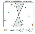
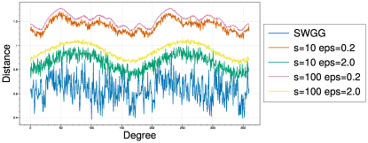
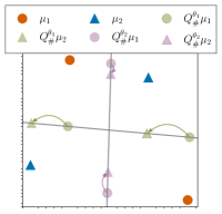
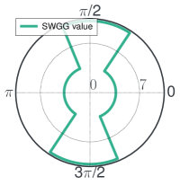
Figure 1: (Left) Empirical distributions with examples of 2 sampled lines (Right) that lead to 2 possible values of SWGG when θ[0,2π]𝜃02𝜋\theta\in[0,2\pi].

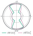
Solving problem in Eq. (9) amounts to optimize over a set of admissible permutations. This problem is hard since SWGG is non convex w.r.t. θ𝜃\theta and piecewise constant, thus not differentiable over 𝕊d1superscript𝕊𝑑1\mathbb{S}^{d-1}. Indeed, as long as the permutations remain the same for different directions θ𝜃\theta, the value of SWGG remains constant. When the permutations change, the objective SWGG "jumps" as illustrated in Fig. 1.

In this section, we tackle this problem by providing an alternative formulation of min-SWGG that allows smoothing the different kinks of SWGG, hence, making min-SWGG amenable to optimization. This formulation relies on Wasserstein generalized geodesics we introduce hereinafter.

We show that this alternative formulation brings in computational advantages and allows establishing some additional topological properties and deriving an efficient optimization scheme. We also provide a new closed form expression of the Wasserstein distance W22(μ1,μ2)subscriptsuperscript𝑊22subscript𝜇1subscript𝜇2W^{2}_{2}(\mu_{1},\mu_{2}) when either μ1subscript𝜇1\mu_{1} or μ2subscript𝜇2\mu_{2} is supported on a line.

4.1 SWGG based on Wasserstein Generalized Geodesics

Wasserstein generalized geodesics (see Supp. B for more details) were first introduced in [4] in order to ensure the convergence of Euler scheme for Wasserstein Gradient Flows. This concept has been used notably in [29, 44] to speed up some computations and to derive some theoretical properties. Generalized geodesic is also highly related with the idea of linearization of the Wasserstein distance via an L2superscript𝐿2L^{2} space [65, 43], see Supp. C for more details on the related works.

Generalized geodesics lay down on a pivot measure ν𝒫2n(d)𝜈subscriptsuperscript𝒫𝑛2superscript𝑑\nu\in\mathcal{P}^{n}_{2}(\mathbb{R}^{d}) to transport the distribution μ1subscript𝜇1\mu_{1} toward μ2subscript𝜇2\mu_{2}. Indeed, one can leverage the optimal transport maps Tνμ1superscript𝑇𝜈subscript𝜇1T^{\nu\to\mu_{1}} and Tνμ2superscript𝑇𝜈subscript𝜇2T^{\nu\to\mu_{2}} to construct a curve tμg12(t)maps-to𝑡subscriptsuperscript𝜇12𝑔𝑡t\mapsto\mu^{1\to 2}_{g}(t) linking μ1subscript𝜇1\mu_{1} to μ2subscript𝜇2\mu_{2} as

μg12(t)=def((1t)Tνμ1+tTνμ2)#ν,t[0,1].formulae-sequencesuperscriptdefsubscriptsuperscript𝜇12𝑔𝑡subscript1𝑡superscript𝑇𝜈subscript𝜇1𝑡superscript𝑇𝜈subscript𝜇2#𝜈for-all𝑡01\mu^{1\to 2}_{g}(t)\stackrel{{\scriptstyle\text{def}}}{{\,\,=\,}}\left((1-t)T^{\nu\to\mu_{1}}+tT^{\nu\to\mu_{2}}\right)_{\#}\nu,\quad\quad\forall t\in[0,1]. (11)

The related generalized Wasserstein mean corresponds to t=0.5𝑡0.5t=0.5 and is denoted μg12subscriptsuperscript𝜇12𝑔\mu^{1\to 2}_{g}.

Intuitively, the optimal transport maps between ν𝜈\nu and μi,i=1,2formulae-sequencesubscript𝜇𝑖𝑖12\mu_{i},i=1,2 give rise to a sub-optimal transport map between μ1subscript𝜇1\mu_{1} and μ2subscript𝜇2\mu_{2}:

Tν12=defTνμ2Tμ1νwith(Tν12)#μ1=μ2.formulae-sequencesuperscriptdefsuperscriptsubscript𝑇𝜈12superscript𝑇𝜈subscript𝜇2superscript𝑇subscript𝜇1𝜈withsubscriptsuperscriptsubscript𝑇𝜈12#subscript𝜇1subscript𝜇2T_{\nu}^{1\to 2}\stackrel{{\scriptstyle\text{def}}}{{\,\,=\,}}T^{\nu\to\mu_{2}}\circ T^{\mu_{1}\to\nu}\quad\text{with}\quad(T_{\nu}^{1\to 2})_{\#}\mu_{1}=\mu_{2}. (12)

One can be interested in the cost induced by the transportation of μ1subscript𝜇1\mu_{1} to μ2subscript𝜇2\mu_{2} via the transport map Tν12superscriptsubscript𝑇𝜈12T_{\nu}^{1\to 2}, known as the ν𝜈\nu-based Wasserstein distance [47] and defined as

Wν2(μ1,μ2)=defd𝒙Tν12(𝒙)22𝑑μ1(𝒙)=2W22(μ1,ν)+2W22(ν,μ2)4W22(μg12,ν).superscriptdefsubscriptsuperscript𝑊2𝜈subscript𝜇1subscript𝜇2subscriptsuperscript𝑑subscriptsuperscriptnorm𝒙superscriptsubscript𝑇𝜈12𝒙22differential-dsubscript𝜇1𝒙2subscriptsuperscript𝑊22subscript𝜇1𝜈2subscriptsuperscript𝑊22𝜈subscript𝜇24subscriptsuperscript𝑊22subscriptsuperscript𝜇12𝑔𝜈W^{2}_{\nu}(\mu_{1},\mu_{2})\stackrel{{\scriptstyle\text{def}}}{{\,\,=\,}}\int_{\mathbb{R}^{d}}\|\boldsymbol{x}-T_{\nu}^{1\to 2}(\boldsymbol{x})\|^{2}_{2}d\mu_{1}(\boldsymbol{x})=2W^{2}_{2}(\mu_{1},\nu)+2W^{2}_{2}(\nu,\mu_{2})-4W^{2}_{2}(\mu^{1\to 2}_{g},\nu). (13)

Notably, the second part of Eq. (13) straddles the square Wasserstein distance with Eq. (3). Remarkably, the computation of Wν2subscriptsuperscript𝑊2𝜈W^{2}_{\nu} can be efficient if the pivot measure ν𝜈\nu is chosen appropriately. As established in Lemma 4.6, it is the case when ν𝜈\nu is supported on a line. Based on these facts, we propose hereafter an alternative formulation of SWGG.

Definition 4.1 (Pivot measure).

Let μ1subscript𝜇1\mu_{1} and μ2𝒫2n(d)subscript𝜇2subscriptsuperscript𝒫𝑛2superscript𝑑\mu_{2}\in\mathcal{P}^{n}_{2}(\mathbb{R}^{d}). We restrict the pivot measure ν𝜈\nu to be the Wasserstein mean of the measures Q#θμ1subscriptsuperscript𝑄𝜃#subscript𝜇1Q^{\theta}_{\#}\mu_{1} and Q#θμ2subscriptsuperscript𝑄𝜃#subscript𝜇2Q^{\theta}_{\#}\mu_{2}:

μθ12=defargminμ𝒫2n(d)W22(Q#θμ1,μ)+W22(μ,Q#θμ2),superscriptdefsubscriptsuperscript𝜇12𝜃subscript𝜇subscriptsuperscript𝒫𝑛2superscript𝑑subscriptsuperscript𝑊22subscriptsuperscript𝑄𝜃#subscript𝜇1𝜇subscriptsuperscript𝑊22𝜇subscriptsuperscript𝑄𝜃#subscript𝜇2\mu^{1\to 2}_{\theta}\stackrel{{\scriptstyle\text{def}}}{{\,\,=\,}}\arg\min_{\mu\in\mathcal{P}^{n}_{2}(\mathbb{R}^{d})}W^{2}_{2}(Q^{\theta}_{\#}\mu_{1},\mu)+W^{2}_{2}(\mu,Q^{\theta}_{\#}\mu_{2}),

where θ𝕊d1𝜃superscript𝕊𝑑1\theta\in\mathbb{S}^{d-1} and Qθ:dd:superscript𝑄𝜃superscript𝑑superscript𝑑Q^{\theta}:\mathbb{R}^{d}\to\mathbb{R}^{d}, 𝒙θ𝒙,θmaps-to𝒙𝜃𝒙𝜃\boldsymbol{x}\mapsto\theta\langle\boldsymbol{x},\theta\rangle is the projection onto the subspace generated by θ𝜃\theta. Moreover μθ12subscriptsuperscript𝜇12𝜃\mu^{1\to 2}_{\theta} is always defined as the middle of a geodesic as in Eq (2).

One shall notice that Q#θμ1subscriptsuperscript𝑄𝜃#subscript𝜇1Q^{\theta}_{\#}\mu_{1} and Q#θμ2subscriptsuperscript𝑄𝜃#subscript𝜇2Q^{\theta}_{\#}\mu_{2} are supported on the line defined by the direction θ𝜃\theta, so is the pivot measure ν=μθ12𝜈subscriptsuperscript𝜇12𝜃\nu=\mu^{1\to 2}_{\theta}. We are now ready to reformulate the metric SWGG.

Proposition 4.2 (SWGG based on generalized geodesics).

Let θ𝕊d1𝜃superscript𝕊𝑑1\theta\in\mathbb{S}^{d-1}, μ1,μ2𝒫2n(d)subscript𝜇1subscript𝜇2subscriptsuperscript𝒫𝑛2superscript𝑑\mu_{1},\mu_{2}\in\mathcal{P}^{n}_{2}(\mathbb{R}^{d}) and μθ12subscriptsuperscript𝜇12𝜃\mu^{1\to 2}_{\theta} be the pivot measure. Let μg,θ12subscriptsuperscript𝜇12𝑔𝜃\mu^{1\to 2}_{g,\theta} be the generalized Wasserstein mean between μ1subscript𝜇1\mu_{1} and μ2𝒫2n(d)subscript𝜇2subscriptsuperscript𝒫𝑛2superscript𝑑\mu_{2}\in\mathcal{P}^{n}_{2}(\mathbb{R}^{d}) with pivot measure μθ12subscriptsuperscript𝜇12𝜃\mu^{1\to 2}_{\theta}. Then,

SWGG22(μ1,μ2,θ)=2W22(μ1,μθ12)+2W22(μθ12,μ2)4W22(μg,θ12,μθ12).superscriptsubscriptSWGG22subscript𝜇1subscript𝜇2𝜃2subscriptsuperscript𝑊22subscript𝜇1subscriptsuperscript𝜇12𝜃2superscriptsubscript𝑊22subscriptsuperscript𝜇12𝜃subscript𝜇24superscriptsubscript𝑊22subscriptsuperscript𝜇12𝑔𝜃subscriptsuperscript𝜇12𝜃\textnormal{SWGG}_{2}^{2}(\mu_{1},\mu_{2},\theta)=2W^{2}_{2}(\mu_{1},\mu^{1\to 2}_{\theta})+2W_{2}^{2}(\mu^{1\to 2}_{\theta},\mu_{2})-4W_{2}^{2}(\mu^{1\to 2}_{g,\theta},\mu^{1\to 2}_{\theta}). (14)

The proof is in Supp.D.1. From Proposition 4.2, SWGG is the μθ12subscriptsuperscript𝜇12𝜃\mu^{1\to 2}_{\theta}-based Wasserstein distance between μ1subscript𝜇1\mu_{1} and μ2subscript𝜇2\mu_{2}. This alternative formulation allows establishing additional properties of min-SWGG.

4.2 Theoretical properties

Additionally to the properties derived in Section 3 (SWGG is a distance and min-SWGG is an upper bound of W22subscriptsuperscript𝑊22W^{2}_{2}), we provide below other theoretical guarantees.

Proposition 4.3 (Weak Convergence).

min-SWGG metricizes the weak convergence in 𝒫2n(d)subscriptsuperscript𝒫𝑛2superscript𝑑\mathcal{P}^{n}_{2}(\mathbb{R}^{d}). In other words, let (μk)ksubscriptsubscript𝜇𝑘𝑘(\mu_{k})_{k\in\mathbb{N}} be a sequence of measures in 𝒫2n(d)subscriptsuperscript𝒫𝑛2superscript𝑑\mathcal{P}^{n}_{2}(\mathbb{R}^{d}) and μ𝒫2n(d)𝜇subscriptsuperscript𝒫𝑛2superscript𝑑\mu\in\mathcal{P}^{n}_{2}(\mathbb{R}^{d}). We have:

μk𝑘,2μmin-SWGG22(μk,μ)𝑘0,iffsubscript𝜇𝑘𝑘2𝜇superscriptsubscriptmin-SWGG22subscript𝜇𝑘𝜇𝑘0\displaystyle\mu_{k}\underset{k}{\overset{\mathcal{L},2}{\longrightarrow}}\mu\iff\textnormal{min-SWGG}_{2}^{2}(\mu_{k},\mu)\underset{k}{\longrightarrow}0,

where ,22\overset{\mathcal{L},2}{\longrightarrow} stands for the weak convergence of measure i.e. df𝑑μkdf𝑑μsubscriptsuperscript𝑑𝑓differential-dsubscript𝜇𝑘subscriptsuperscript𝑑𝑓differential-d𝜇\int_{\mathbb{R}^{d}}fd\mu_{k}\to\int_{\mathbb{R}^{d}}fd\mu for all continuous bounded functions f𝑓f.

Beyond the weak convergence, min-SWGG possesses the translation property, i.e. the translations can be factored out as the Wasserstein distance does (see [53, remark 2.19] for a recall).

Proposition 4.4 (Translation).

Let Tusuperscript𝑇𝑢T^{u} (resp. Tvsuperscript𝑇𝑣T^{v}) be the map 𝒙𝒙𝒖maps-to𝒙𝒙𝒖\boldsymbol{x}\mapsto\boldsymbol{x}-\boldsymbol{u} (resp. 𝒙𝒙𝒗maps-to𝒙𝒙𝒗\boldsymbol{x}\mapsto\boldsymbol{x}-\boldsymbol{v}), with 𝒖,𝒗𝒖𝒗\boldsymbol{u},\boldsymbol{v} vectors of dsuperscript𝑑\mathbb{R}^{d}. We have:

min-SWGG22(T#uμ1,T#vμ2)=superscriptsubscriptmin-SWGG22subscriptsuperscript𝑇𝑢#subscript𝜇1subscriptsuperscript𝑇𝑣#subscript𝜇2absent\displaystyle\textnormal{min-SWGG}_{2}^{2}(T^{u}_{\#}\mu_{1},T^{v}_{\#}\mu_{2})= min-SWGG22(μ1,μ2)+𝒖𝒗222𝒖𝒗,𝒎𝟏𝒎𝟐superscriptsubscriptmin-SWGG22subscript𝜇1subscript𝜇2superscriptsubscriptnorm𝒖𝒗222𝒖𝒗subscript𝒎1subscript𝒎2\displaystyle\leavevmode\nobreak\ \textnormal{min-SWGG}_{2}^{2}(\mu_{1},\mu_{2})+\|\boldsymbol{u}-\boldsymbol{v}\|_{2}^{2}-2\langle\boldsymbol{u}-\boldsymbol{v},\boldsymbol{m_{1}}-\boldsymbol{m_{2}}\rangle

where 𝒎𝟏=d𝒙𝑑μ1(𝒙)subscript𝒎1subscriptsuperscript𝑑𝒙differential-dsubscript𝜇1𝒙\boldsymbol{m_{1}}=\int_{\mathbb{R}^{d}}\boldsymbol{x}d\mu_{1}(\boldsymbol{x}) and 𝒎𝟐=d𝒙𝑑μ2(𝒙)subscript𝒎2subscriptsuperscript𝑑𝒙differential-dsubscript𝜇2𝒙\boldsymbol{m_{2}}=\int_{\mathbb{R}^{d}}\boldsymbol{x}d\mu_{2}(\boldsymbol{x}) are the means of μ1subscript𝜇1\mu_{1}, μ2subscript𝜇2\mu_{2}.

This property is useful in some applications such as shape matching, in which translation invariances are sought.

The proofs of the two Propositions are deferred to Supp. D.2 and D.3.

Remark 4.5 (Equality).

min-SWGG and W22subscriptsuperscript𝑊22W^{2}_{2} are equal in different cases. First, [43] showed that it is the case whenever μ1subscript𝜇1\mu_{1} is the shift and scaling of μ2subscript𝜇2\mu_{2} (see Supp. C.1 for a full discussion). In Lemma 4.6, we will state that it is also the case if one of the two distributions is supported on a line.

4.3 Efficient computation of SWGG

SWGG defined in Eq. (14) involves computing three WDs that are fast to compute, with an overall 𝒪(dn+nlogn)𝒪𝑑𝑛𝑛𝑛\mathcal{O}(dn+n\log n) complexity, as detailed below. Building on this result, we provide an optimization scheme that allows optimizing over θ𝜃\theta with 𝒪(sdn+snlogsn)𝒪𝑠𝑑𝑛𝑠𝑛𝑠𝑛\mathcal{O}(sdn+sn\log sn) operations at each iteration, with s𝑠s a (small) integer. We first start by giving a new closed form expression of the WD whenever one distribution is supported on a line, that proves useful for deriving an efficient computation scheme.

New closed form of the WD.

The following lemma states that W22(μ1,μ2)subscriptsuperscript𝑊22subscript𝜇1subscript𝜇2W^{2}_{2}(\mu_{1},\mu_{2}) admits a closed form whenever μ2subscript𝜇2\mu_{2} is supported on a line.

This lemma leverages the computation of the WD between μ2subscript𝜇2\mu_{2} and the orthogonal projection of μ1subscript𝜇1\mu_{1} onto the linear subspace defined by the line. Additionally, it provides an explicit formulation for the optimal transport map T12superscript𝑇12T^{1\to 2}.

Lemma 4.6.

Let μ1,μ2subscript𝜇1subscript𝜇2\mu_{1},\mu_{2} in 𝒫2n(d)subscriptsuperscript𝒫𝑛2superscript𝑑\mathcal{P}^{n}_{2}(\mathbb{R}^{d}) with μ2subscript𝜇2\mu_{2} supported on a line of direction θ𝕊d1𝜃superscript𝕊𝑑1\theta\in\mathbb{S}^{d-1}. We have:

W22(μ1,μ2)=W22(μ1,Q#θμ1)+W22(Q#θμ1,μ2)subscriptsuperscript𝑊22subscript𝜇1subscript𝜇2subscriptsuperscript𝑊22subscript𝜇1superscriptsubscript𝑄#𝜃subscript𝜇1subscriptsuperscript𝑊22superscriptsubscript𝑄#𝜃subscript𝜇1subscript𝜇2W^{2}_{2}(\mu_{1},\mu_{2})=W^{2}_{2}(\mu_{1},Q_{\#}^{\theta}\mu_{1})+W^{2}_{2}(Q_{\#}^{\theta}\mu_{1},\mu_{2}) (15)

with Qθsuperscript𝑄𝜃Q^{\theta} as in Def. 4.1. Note that W22(μ1,Q#θμ1)=1n𝒙iQθ(𝒙i)22subscriptsuperscript𝑊22subscript𝜇1subscriptsuperscript𝑄𝜃#subscript𝜇11𝑛subscriptsuperscriptnormsubscript𝒙𝑖superscript𝑄𝜃subscript𝒙𝑖22W^{2}_{2}(\mu_{1},Q^{\theta}_{\#}\mu_{1})=\frac{1}{n}\sum\|\boldsymbol{x}_{i}-Q^{\theta}(\boldsymbol{x}_{i})\|^{2}_{2} and W22(Q#θμ1,μ2)=W22(P#θμ1,P#θμ2)subscriptsuperscript𝑊22superscriptsubscript𝑄#𝜃subscript𝜇1subscript𝜇2subscriptsuperscript𝑊22superscriptsubscript𝑃#𝜃subscript𝜇1superscriptsubscript𝑃#𝜃subscript𝜇2W^{2}_{2}(Q_{\#}^{\theta}\mu_{1},\mu_{2})=W^{2}_{2}(P_{\#}^{\theta}\mu_{1},P_{\#}^{\theta}\mu_{2}) are the WD between 1D distributions. Additionally, the optimal transport map is given by T12=TQ#θμ1μ2Tμ1Q#θμ1=TQ#θμ1μ2Qθsuperscript𝑇12superscript𝑇subscriptsuperscript𝑄𝜃#subscript𝜇1subscript𝜇2superscript𝑇subscript𝜇1subscriptsuperscript𝑄𝜃#subscript𝜇1superscript𝑇subscriptsuperscript𝑄𝜃#subscript𝜇1subscript𝜇2superscript𝑄𝜃T^{1\to 2}=T^{Q^{\theta}_{\#}\mu_{1}\to\mu_{2}}\circ T^{\mu_{1}\to Q^{\theta}_{\#}\mu_{1}}=T^{Q^{\theta}_{\#}\mu_{1}\to\mu_{2}}\circ Q^{\theta}. In particular, the map T12superscript𝑇12T^{1\to 2} can be obtained via the permutations of the 1D distributions P#θμ1subscriptsuperscript𝑃𝜃#subscript𝜇1P^{\theta}_{\#}\mu_{1} and P#θμ2subscriptsuperscript𝑃𝜃#subscript𝜇2P^{\theta}_{\#}\mu_{2}. The proof is provided in Supp. D.4.

Efficient computation of SWGG.

Eq. (14) is defined as the Wasserstein distance between a distribution (either μ1subscript𝜇1\mu_{1} or μ2subscript𝜇2\mu_{2} or μg,θ12)\mu^{1\to 2}_{g,\theta}) and a distribution supported on a line (μθ12subscriptsuperscript𝜇12𝜃\mu^{1\to 2}_{\theta}). As detailed in Supp. D.5, computation of Eq. (14) involves three Wasserstein distances between distributions and their projections: i) W22(μ1,Q#θμ1)subscriptsuperscript𝑊22subscript𝜇1subscriptsuperscript𝑄𝜃#subscript𝜇1W^{2}_{2}(\mu_{1},Q^{\theta}_{\#}\mu_{1}), ii) W22(μ2,Q#θμ2)subscriptsuperscript𝑊22subscript𝜇2subscriptsuperscript𝑄𝜃#subscript𝜇2W^{2}_{2}(\mu_{2},Q^{\theta}_{\#}\mu_{2}), iii) W22(μg,θ12,μθ12)subscriptsuperscript𝑊22subscriptsuperscript𝜇12𝑔𝜃subscriptsuperscript𝜇12𝜃W^{2}_{2}(\mu^{1\to 2}_{g,\theta},\mu^{1\to 2}_{\theta}), and a one dimensional Wasserstein distance W22(P#θμ1,P#θμ2)superscriptsubscript𝑊22subscriptsuperscript𝑃𝜃#subscript𝜇1subscriptsuperscript𝑃𝜃#subscript𝜇2W_{2}^{2}(P^{\theta}_{\#}\mu_{1},P^{\theta}_{\#}\mu_{2}), resulting in a 𝒪(dn+nlogn)𝒪𝑑𝑛𝑛𝑛\mathcal{O}(dn+n\log n) complexity.

Optimization scheme for min-SWGG.

The term W22(μg,θ12,μθ12)superscriptsubscript𝑊22subscriptsuperscript𝜇12𝑔𝜃subscriptsuperscript𝜇12𝜃W_{2}^{2}(\mu^{1\to 2}_{g,\theta},\mu^{1\to 2}_{\theta}) in Eq. (14) is not continuous w.r.t. θ𝜃\theta. Indeed, the generalized mean μg,θ12subscriptsuperscript𝜇12𝑔𝜃\mu^{1\to 2}_{g,\theta} depends only on the transport maps Tμθ12μ1superscript𝑇subscriptsuperscript𝜇12𝜃subscript𝜇1T^{\mu^{1\to 2}_{\theta}\to\mu_{1}} and Tμθ12μ2superscript𝑇subscriptsuperscript𝜇12𝜃subscript𝜇2T^{\mu^{1\to 2}_{\theta}\to\mu_{2}}, which remain constant as long as different projection directions θ𝜃\theta lead to the same permutations σθsubscript𝜎𝜃\sigma_{\theta} and τθsubscript𝜏𝜃\tau_{\theta}. Hence, we rely on a smooth surrogate μg,θ12~~subscriptsuperscript𝜇12𝑔𝜃\widetilde{\mu^{1\to 2}_{g,\theta}} of the generalized mean and we aim to minimize the following objective function:

SWGG22~(μ1,μ2,θ)=def2W22(μ1,μθ12)+2W22(μθ12,μ2)4W22(μg,θ12~,μθ12).superscriptdef~superscriptsubscriptSWGG22subscript𝜇1subscript𝜇2𝜃2subscriptsuperscript𝑊22subscript𝜇1subscriptsuperscript𝜇12𝜃2superscriptsubscript𝑊22subscriptsuperscript𝜇12𝜃subscript𝜇24superscriptsubscript𝑊22~subscriptsuperscript𝜇12𝑔𝜃subscriptsuperscript𝜇12𝜃\widetilde{\textnormal{SWGG}_{2}^{2}}({\mu}_{1},{\mu}_{2},\theta)\stackrel{{\scriptstyle\text{def}}}{{\,\,=\,}}2W^{2}_{2}(\mu_{1},\mu^{1\to 2}_{\theta})+2W_{2}^{2}(\mu^{1\to 2}_{\theta},\mu_{2})-4{W_{2}^{2}}(\widetilde{\mu^{1\to 2}_{g,\theta}},\mu^{1\to 2}_{\theta}). (16)

To define μg,θ12~~subscriptsuperscript𝜇12𝑔𝜃\widetilde{\mu^{1\to 2}_{g,\theta}}, one option would be to use entropic maps in Eq. (11) but at the price of a quadratic time complexity. We rather build upon the blurred Wasserstein distance [26] to define μg,θ12~~subscriptsuperscript𝜇12𝑔𝜃\widetilde{\mu^{1\to 2}_{g,\theta}} as it can be seen as an efficient surrogate of entropic transport plans in 1D. In one dimensional setting, μg,θ12~~subscriptsuperscript𝜇12𝑔𝜃\widetilde{\mu^{1\to 2}_{g,\theta}} can be approximated efficiently by adding an empirical Gaussian noise followed by a sorting pass. In our case, it resorts in making s𝑠s copies of each sorted projection Pθ(𝒙σ(i))superscript𝑃𝜃subscript𝒙𝜎𝑖P^{\theta}(\boldsymbol{x}_{\sigma(i)}) and Pθ(𝒚τ(i))superscript𝑃𝜃subscript𝒚𝜏𝑖P^{\theta}(\boldsymbol{y}_{\tau(i)}) respectively, to add an empirical Gaussian noise of deviation ϵ/2italic-ϵ2\sqrt{\epsilon}/2 and to compute averages of sorted blurred copies 𝒙σsssubscriptsuperscript𝒙𝑠superscript𝜎𝑠\boldsymbol{x}^{s}_{\sigma^{s}}, 𝒚τsssubscriptsuperscript𝒚𝑠superscript𝜏𝑠\boldsymbol{y}^{s}_{\tau^{s}}. We finally have (μg,θ12~)i=12sk=(i1)s+1is𝒙σs(k)s+𝒚τs(k)ssubscript~subscriptsuperscript𝜇12𝑔𝜃𝑖12𝑠superscriptsubscript𝑘𝑖1𝑠1𝑖𝑠subscriptsuperscript𝒙𝑠superscript𝜎𝑠𝑘subscriptsuperscript𝒚𝑠superscript𝜏𝑠𝑘(\widetilde{\mu^{1\to 2}_{g,\theta}})_{i}=\frac{1}{2s}\sum_{k=(i-1)s+1}^{is}\boldsymbol{x}^{s}_{\sigma^{s}(k)}+\boldsymbol{y}^{s}_{\tau^{s}(k)}. [26] showed that this blurred WD has the same asymptotic properties as the Sinkhorn divergence.

The surrogate SWGG~(μ1,μ2,θ)~SWGGsubscript𝜇1subscript𝜇2𝜃\widetilde{\textnormal{SWGG}}({\mu}_{1},{\mu}_{2},\theta) is smoother w.r.t. θ𝜃\theta and can thus be optimized using gradient descent, converging towards a local minima. Once the optimal direction θsuperscript𝜃\theta^{*} is found, min-SWGG resorts to be the solution provided by SWGG(μ1,μ2,θ)SWGGsubscript𝜇1subscript𝜇2superscript𝜃\textnormal{SWGG}(\mu_{1},\mu_{2},\theta^{*}). Fig. 2 illustrates the effect of the smoothing on a toy example and more details are given in Supp. D.6. The computation of SWGG~(μ1,μ2,θ)~SWGGsubscript𝜇1subscript𝜇2𝜃\widetilde{\textnormal{SWGG}}({\mu}_{1},{\mu}_{2},\theta) is summarized in Alg. 1.

Algorithm 1 Computing SWGG22~~superscriptsubscriptSWGG22\widetilde{\textnormal{SWGG}_{2}^{2}}(μ1,μ2,θ)subscript𝜇1subscript𝜇2𝜃({\mu}_{1},{\mu}_{2},\theta)
μ1=1nδ𝒙isubscript𝜇11𝑛subscript𝛿subscript𝒙𝑖\mu_{1}=\frac{1}{n}\sum\delta_{\boldsymbol{x}_{i}}, μ2=1nδ𝒚isubscript𝜇21𝑛subscript𝛿subscript𝒚𝑖\mu_{2}=\frac{1}{n}\sum\delta_{\boldsymbol{y}_{i}}, θ𝕊d1𝜃superscript𝕊𝑑1\theta\in\mathbb{S}^{d-1}, s+𝑠subscripts\in\mathbb{N}_{+} and ϵ+italic-ϵsubscript\epsilon\in\mathbb{R}_{+}
σ,τ𝜎𝜏absent{\sigma},{\tau}\leftarrow ascending ordering of (Pθ(𝒙i))isubscriptsuperscript𝑃𝜃subscript𝒙𝑖𝑖(P^{\theta}(\boldsymbol{x}_{i}))_{i}, (Qθ(𝒚i))isubscriptsuperscript𝑄𝜃subscript𝒚𝑖𝑖(Q^{\theta}(\boldsymbol{y}_{i}))_{i}
𝒙sssuperscript𝒙𝑠𝑠\boldsymbol{x}^{s}\leftarrow s copies of (𝒙σ(i))isubscriptsubscript𝒙𝜎𝑖𝑖(\boldsymbol{x}_{\sigma(i)})_{i}, 𝒚sssuperscript𝒚𝑠𝑠\boldsymbol{y}^{s}\leftarrow s copies of (𝒚τ(i))isubscriptsubscript𝒚𝜏𝑖𝑖(\boldsymbol{y}_{\tau(i)})_{i}
σs,τssuperscript𝜎𝑠superscript𝜏𝑠absent{\sigma^{s}},{\tau^{s}}\leftarrow ascending ordering of 𝒙s,θ+𝝃superscript𝒙𝑠𝜃𝝃\langle\boldsymbol{x}^{s},\theta\rangle+\boldsymbol{\xi}, 𝒚s,θ+𝝃superscript𝒚𝑠𝜃𝝃\langle\boldsymbol{y}^{s},\theta\rangle+\boldsymbol{\xi} for ξi𝒩(0,ϵ/2)similar-tosubscript𝜉𝑖𝒩0italic-ϵ2\xi_{i}\sim\mathcal{N}(0,\epsilon/2), isnfor-all𝑖𝑠𝑛\forall i\leq sn
a2ni(𝒙iQθ(𝒙i)22+𝒚iQθ(𝒚i)22)a\leftarrow\frac{2}{n}\sum_{i}\left(\bigl{\|}\boldsymbol{x}_{i}-Q^{\theta}(\boldsymbol{x}_{i})\|^{2}_{2}+\|\boldsymbol{y}_{i}-Q^{\theta}(\boldsymbol{y}_{i})\|^{2}_{2}\right) \triangleright 2W22(μ1,Q#θμ1)+2W22(μ2,Q#θμ2)2subscriptsuperscript𝑊22subscript𝜇1subscriptsuperscript𝑄𝜃#subscript𝜇12subscriptsuperscript𝑊22subscript𝜇2subscriptsuperscript𝑄𝜃#subscript𝜇22W^{2}_{2}(\mu_{1},Q^{\theta}_{\#}\mu_{1})+2W^{2}_{2}(\mu_{2},Q^{\theta}_{\#}\mu_{2})
b2niPθ(𝒙σ(i))+Pθ(𝒙τ(i))22𝑏2𝑛subscript𝑖subscriptsuperscriptdelimited-∥∥superscript𝑃𝜃subscript𝒙𝜎𝑖superscript𝑃𝜃subscript𝒙𝜏𝑖22b\leftarrow\frac{2}{n}\sum_{i}\bigl{\|}P^{\theta}(\boldsymbol{x}_{\sigma(i)})+P^{\theta}(\boldsymbol{x}_{\tau(i)})\bigr{\|}^{2}_{2} \triangleright 2W22(P#θμ1,P#θμ2)2subscriptsuperscript𝑊22subscriptsuperscript𝑃𝜃#subscript𝜇1subscriptsuperscript𝑃𝜃#subscript𝜇22W^{2}_{2}(P^{\theta}_{\#}\mu_{1},P^{\theta}_{\#}\mu_{2})
c4ni12(Qθ(𝒙σ(i))+Qθ(𝒚τ(i)))12sk=(i1)s+1is(𝒙σs(k)s+𝒚τs(k)s)22𝑐4𝑛subscript𝑖subscriptsuperscriptdelimited-∥∥12superscript𝑄𝜃subscript𝒙𝜎𝑖superscript𝑄𝜃subscript𝒚𝜏𝑖12𝑠superscriptsubscript𝑘𝑖1𝑠1𝑖𝑠subscriptsuperscript𝒙𝑠superscript𝜎𝑠𝑘subscriptsuperscript𝒚𝑠superscript𝜏𝑠𝑘22c\leftarrow\frac{4}{n}\sum\limits_{i}\bigl{\|}\frac{1}{2}(Q^{\theta}(\boldsymbol{x}_{\sigma(i)})+Q^{\theta}(\boldsymbol{y}_{\tau(i)}))-\frac{1}{2s}\sum\limits_{k=(i-1)s+1}^{is}(\boldsymbol{x}^{s}_{\sigma^{s}(k)}+\boldsymbol{y}^{s}_{\tau^{s}(k)})\bigr{\|}^{2}_{2} \triangleright 4W22(μg,θ12~,μθ12)4subscriptsuperscript𝑊22~subscriptsuperscript𝜇12𝑔𝜃subscriptsuperscript𝜇12𝜃4W^{2}_{2}(\widetilde{\mu^{1\to 2}_{g,\theta}},\mu^{1\to 2}_{\theta})
Output a+bc𝑎𝑏𝑐a+b-c
Refer to caption
Refer to caption
Refer to caption
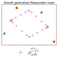
Figure 2: Illustration of the smoothing effect in the same setting as in Fig. 1. (Left) Two sets of generalized Wasserstein means are possible, depending on the direction of the sampled line w.r.t. θ1subscript𝜃1\theta_{1} and θ2subscript𝜃2\theta_{2}, giving rise to 2 different values for SWGG. (Middle) The surrogate provides a smooth transition between the two sets of generalized Wasserstein means as the direction θ𝜃\theta changes, (Right) providing a smooth approximation of SWGG that is amenable to optimization.

5 Experiments

We highlight that min-SWGG is fast to compute, gives an approximation of the WD and the associated transport plan. We start by comparing the random search and the gradient descent schemes for finding the optimal direction in subsection 5.1. Subsection 5.2 illustrates the weak convergence property of min-SWGG through a gradient flow application to match distributions. We then implement an efficient algorithm for colorization of gray scale images in 5.3, thanks to the new closed form expression of the WD. We finally evaluate min-SWGG in a shape matching context in subsection 5.4. When possible from the context, we compare min-SWGG with the main methods for approximating the WD namely SW, max-SW, Sinkhorn [23], factored coupling [29] and subspace robust WD (SRW) [52]. Supp. E provides additional results on the behavior of min-SWGG and experiments on other tasks such as color transfer or on data sets distance computation. All the code is available at 111https://github.com/MaheyG/SWGG

5.1 Computing min-SWGG

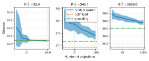
Let consider Gaussian distributions in dimensions d{2,20,200}𝑑220200d\in\{2,20,200\}. We first sample n=1000𝑛1000n=1000 points from each distribution to define μ1subscript𝜇1\mu_{1} and μ2subscript𝜇2\mu_{2}. We then compute min-SWGG22(μ1,μ2)superscriptsubscriptmin-SWGG22subscript𝜇1subscript𝜇2\textnormal{min-SWGG}_{2}^{2}(\mu_{1},\mu_{2}) computed using different schemes, either by random search, by simulated annealing [54] or by gradient descent. We report the obtained results in Fig. 3 (left). For the random search scheme, we repeat each experiment 20 times and we plot the average value of min-SWGG ±plus-or-minus\pm 2 times the standard deviation.

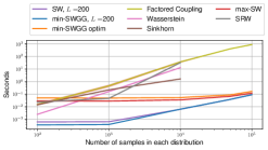
For the gradient descent, we select a random initial θ𝜃\theta. We observe that, in low dimension, all schemes provide similar values of min-SWGG. When the dimension increases, optimizing the direction θ𝜃\theta yields a more accurate approximation of the true Wasserstein distance (see plots’ title in Fig. 3). On Fig. 3 (right), we compare the empirical runtime evaluation for min-SWGG with different competitors for d=3𝑑3d=3 and using n𝑛n samples from Gaussian distributions, with n{102,103,104,5×104,105}𝑛superscript102superscript103superscript1045superscript104superscript105n\in\{10^{2},10^{3},10^{4},5\times 10^{4},10^{5}\}. We observe that, as expected, min-SWGG with random search is as fast as SW with a super linear time complexity. With the optimization process, it is faster than SRW for a given number of samples. We also note that SRW is more demanding in memory and hence does not scale as well as min-SWGG. We give more details on this experimentation and a comparison with competitors in Supp. E.2.

Refer to caption
Refer to caption
Figure 3: (Left) evolution of min-SWGG with different numbers of projections and with the dimension d𝑑d in {2,20,200}220200\{2,20,200\}. (Right) Runtimes.

5.2 Gradient Flows

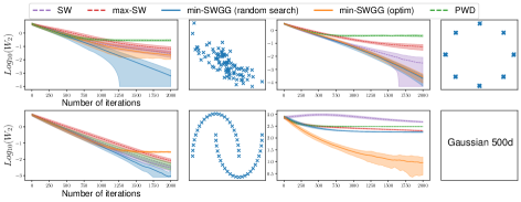
We highlight the weak convergence property of min-SWGG. Initiating from a random initial distribution, we aim to move the particles of a source distribution μ1subscript𝜇1\mu_{1} towards a target one μ2subscript𝜇2\mu_{2} by reducing the objective min-SWGG22(μ1,μ2)superscriptsubscriptmin-SWGG22subscript𝜇1subscript𝜇2\textnormal{min-SWGG}_{2}^{2}(\mu_{1},\mu_{2}) at each step. We compare both variants of min-SWGG against SW, max-SW and PWD, relying on the code provided in [37] for running the experiment; we report the results on Fig. 4. We consider several target distributions, representing diverse scenarios and fix n=100𝑛100n=100. We run each experiment 10 times and report the mean ±plus-or-minus\pm the standard deviation. In every case, one can see that μ1subscript𝜇1\mu_{1} moves towards μ2subscript𝜇2\mu_{2} and that all methods tend to have similar behavior. One can notice though that, for the distributions in d=500𝑑500d=500 dimensional space, min-SWGG computed with the optimization scheme leads to the best alignment of the distributions.

Refer to caption
Figure 4: Log of the WD between different source and target distributions as a function of the number of iterations.

5.3 Gray scale image colorization

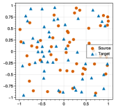
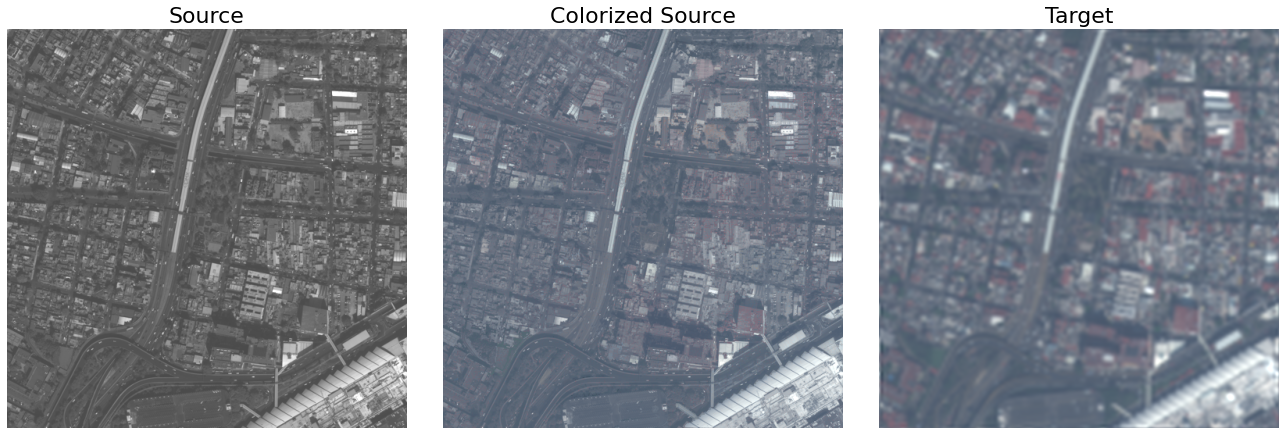
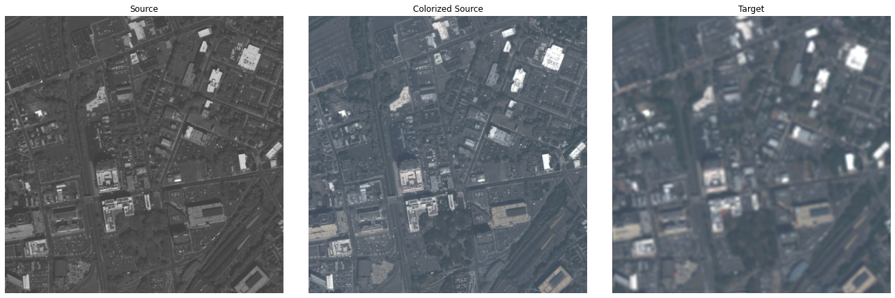
Lemma 4.6 states that the WD has a closed form when one of the 2 distributions is supported on a line, allowing us to compute the WD and the OT map with a complexity of 𝒪(dn+nlogn)𝒪𝑑𝑛𝑛𝑛\mathcal{O}(dn+n\log n). This particular situation arises for instance with RBG images (μ1,μ2𝒫2n(3)subscript𝜇1subscript𝜇2superscriptsubscript𝒫2𝑛superscript3\mu_{1},\mu_{2}\in\mathcal{P}_{2}^{n}(\mathbb{R}^{3})), where black and white images are supported on a line (the line of grays). One can address the problem of image colorization through color transfer [25], where a black and white image is the source and a colorful image the target. Our fast procedure allows considering large images without sub-sampling with a reasonable computation time. Fig. 5 gives an example of colorization of an image of size 1280×\times1024 that was computed in less than 0.2 second, while being totally untractable for the 𝒪(n3logn)𝒪superscript𝑛3𝑛\mathcal{O}(n^{3}\log n) solver of WD.

Refer to caption
Figure 5: Cloud point source and target (left) colorization of image (right).

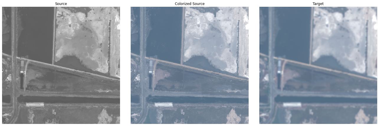
This procedure can be lifted to pan-sharpening [64] where one aims to construct a super-resolution multi-chromatic satellite image with the help of a super-resolution mono-chromatic image (source) and a low-resolution multi-chromatic image (target). Obtained results are given in the Supp. E.4.

5.4 Point clouds registration

Iterative Closest Point (ICP) is an algorithm for aligning point clouds based on their geometries [7]. Roughly, its most popular version defines a one-to-one correspondence between point clouds, computes a rigid transformation (namely translation, rotation or reflection), moves the source point clouds using the transformation, and iterates the procedure until convergence. The rigid transformation is the solution of the Procrustes problem i.e. argmin(Ω,t)O(d)×dΩ(𝑿t)𝒀22subscriptΩ𝑡𝑂𝑑superscript𝑑superscriptsubscriptnormΩ𝑿𝑡𝒀22\arg\min_{(\Omega,t)\in O(d)\times\mathbb{R}^{d}}\|\Omega(\boldsymbol{X}-t)-\boldsymbol{Y}\|_{2}^{2}, where 𝑿,𝒀𝑿𝒀\boldsymbol{X},\boldsymbol{Y} are the source and the target cloud points and O(d)𝑂𝑑O(d) the space of orthogonal matrices of dimension d𝑑d. This Procrustes problem can be solved using a SVD [59] for instance.

We perform the ICP algorithm with different variants to compute the one-to-one correspondence: neareast neighbor (NN) correspondence, OT transport map (for small size datasets) and min-SWGG transport map. Note that SW, PWD, SRW, factored coupling and Sinkhorn cannot be run in this context where a one-to-one correspondence is mandatory; subspace detours [44] are irrelevant in this context (see Supp. E.5). We evaluate the results of the ICP algorithm in terms of: i) the quality of the final alignment, measured by the Sinkhorn divergence between the re-aligned and target point cloud; ii) the speed of the algorithm given by the running time until convergence. We consider 3 datasets of different sizes. The results are shown in Table 1 and more details about the setup, can be found in Supp. E.5. In Supp. E.5 we give a deeper analysis of the results, notably with different criteria for the final assignment, namely the Chamfer and the Frobenius distance. One can see that the assignment provided by OT-based methods is better than NN. min-SWGG allows working with large datasets, while OT fails to provide a solution for n=150000𝑛150000n=150000.

[Uncaptioned image]
n𝑛n 500 3000 150 000
NN 3.54 (0.02) 96.9 (0.30) 23.3 (59.37)
OT 0.32 (0.18) 48.4 (58.46) \cdot
min-SWGG 0.05 (0.04) 37.6 (0.90) 6.7 (105.75)
Table 1: Sinkhorn Divergence between final transformation on the source and the target. Timings in seconds are into parenthesis. Best values are boldfaced. An example of a point clouds (n=3000𝑛3000n=3000) is provided on the left.

6 Conclusion

In this paper, we hinge on the properties of sliced Wasserstein distance and on the Wasserstein generalized geodesics to define min-SWGG, a new upper bound of the Wasserstein distance that comes with an associated transport map. Topological properties of SWGG are provided, showing that it defines a metric and that min-SWGG metrizes the weak convergence of measure. We also propose two algorithms for computing min-SWGG, either through a random search scheme or a gradient descent procedure after smoothing the generalized geodesics definition of min-SWGG. We illustrate its behavior in several experimental setups, notably showcasing its interest in applications where a transport map is needed.
The set of permutations covered by min-SWGG is the one induced by projections and permutations on the line. It is a subset of the original Birkhoff polytope and it would be interesting to characterize how these two sets relates. In particular, in the case of empirical realizations of continuous distributions, the behavior of min-SWGG, when n𝑛n grows, needs to be investigated. In addition, the fact that min-SWGG and WD coincide when d>2n𝑑2𝑛d>2n calls for embedding the distributions in higher dimensional spaces to benefit from the greater expressive power of projection onto the line. Another important consideration is to establish a theoretical upper bound for min-SWGG.

Acknowledgments

The authors gratefully acknowledge the financial support of the French Agence Nationale de la Recherche (ANR), under grant ANR-20-CHIA-0021-01 (project RAIMO222https://chaire-raimo.github.io/), grant ANR-20-CHIA-0030 (project OTTOPIA) and grant ANR-18-CE23-0022-01 (project MULTISCALE). Clément Bonet is supported by the project DynaLearn from Labex CominLabs and Région Bretagne ARED DLearnMe.

References

  • [1] Aleksandr Danilovich Alexandrov. A theorem on triangles in a metric space and some of its applications. Trudy Mat. Inst. Steklov., 38:5–23, 1951.
  • [2] Jason Altschuler, Jonathan Niles-Weed, and Philippe Rigollet. Near-linear time approximation algorithms for optimal transport via sinkhorn iteration. Advances in neural information processing systems, 30, 2017.
  • [3] David Alvarez-Melis and Nicolo Fusi. Geometric dataset distances via optimal transport. Advances in Neural Information Processing Systems, 33:21428–21439, 2020.
  • [4] Luigi Ambrosio, Nicola Gigli, and Giuseppe Savaré. Gradient flows: in metric spaces and in the space of probability measures. Springer Science & Business Media, 2005.
  • [5] Martin Arjovsky, Soumith Chintala, and Léon Bottou. Wasserstein generative adversarial networks. In International conference on machine learning, pages 214–223. PMLR, 2017.
  • [6] Arturs Backurs, Yihe Dong, Piotr Indyk, Ilya Razenshteyn, and Tal Wagner. Scalable nearest neighbor search for optimal transport. In International Conference on Machine Learning, pages 497–506. PMLR, 2020.
  • [7] Paul J Besl and Neil D McKay. Method for registration of 3-d shapes. In Sensor fusion IV: control paradigms and data structures, volume 1611, pages 586–606. Spie, 1992.
  • [8] Garrett Birkhoff. Tres observaciones sobre el algebra lineal. Univ. Nac. Tucuman, Ser. A, 5:147–154, 1946.
  • [9] Nicolas Bonneel and David Coeurjolly. Spot: sliced partial optimal transport. ACM Transactions on Graphics (TOG), 38(4):1–13, 2019.
  • [10] Nicolas Bonneel, Julien Rabin, Gabriel Peyré, and Hanspeter Pfister. Sliced and radon wasserstein barycenters of measures. Journal of Mathematical Imaging and Vision, 51(1):22–45, 2015.
  • [11] Nicolas Bonneel, Michiel Van De Panne, Sylvain Paris, and Wolfgang Heidrich. Displacement interpolation using lagrangian mass transport. In Proceedings of the 2011 SIGGRAPH Asia conference, pages 1–12, 2011.
  • [12] Yann Brenier. Polar factorization and monotone rearrangement of vector-valued functions. Communications on pure and applied mathematics, 44(4):375–417, 1991.
  • [13] Giuseppe Buttazzo, Guillaume Carlier, and Katharina Eichinger. Wasserstein interpolation with constraints and application to a parking problem. arXiv preprint arXiv:2207.14261, 2022.
  • [14] Luis A Caffarelli. Monotonicity properties of optimal transportation¶ and the fkg and related inequalities. Communications in Mathematical Physics, 214(3):547–563, 2000.
  • [15] Laetitia Chapel, Mokhtar Z Alaya, and Gilles Gasso. Partial optimal tranport with applications on positive-unlabeled learning. In Advances in Neural Information Processing Systems, volume 33, pages 2903–2913, 2020.
  • [16] Rui Chibante. Simulated annealing: theory with applications. BoD–Books on Demand, 2010.
  • [17] Tarin Clanuwat, Mikel Bober-Irizar, Asanobu Kitamoto, Alex Lamb, Kazuaki Yamamoto, and David Ha. Deep learning for classical japanese literature. In Neural Information Processing Systems Machine Learning for Creativity and Design Workshop, 2018.
  • [18] Gregory Cohen, Saeed Afshar, Jonathan Tapson, and Andre Van Schaik. EMNIST: Extending MNIST to handwritten letters. In 2017 international joint conference on neural networks (IJCNN), pages 2921–2926, 2017.
  • [19] Nicolas Courty, Rémi Flamary, Devis Tuia, and Alain Rakotomamonjy. Optimal transport for domain adaptation. IEEE Transactions on Pattern Analysis and Machine Intelligence, 39(9):1853–1865, 2017.
  • [20] Thomas M Cover. The number of linearly inducible orderings of points in d-space. SIAM Journal on Applied Mathematics, 15(2):434–439, 1967.
  • [21] Katy Craig. The exponential formula for the wasserstein metric. ESAIM: Control, Optimisation and Calculus of Variations, 22(1):169–187, 2016.
  • [22] JA Cuesta-Albertos, C Matrán, and Araceli Tuero-Diaz. Optimal transportation plans and convergence in distribution. journal of multivariate analysis, 60(1):72–83, 1997.
  • [23] Marco Cuturi. Sinkhorn distances: Lightspeed computation of optimal transport. Advances in neural information processing systems, 26, 2013.
  • [24] Ishan Deshpande, Yuan-Ting Hu, Ruoyu Sun, Ayis Pyrros, Nasir Siddiqui, Sanmi Koyejo, Zhizhen Zhao, David Forsyth, and Alexander G Schwing. Max-sliced wasserstein distance and its use for gans. In Proceedings of the IEEE/CVF Conference on Computer Vision and Pattern Recognition, pages 10648–10656, 2019.
  • [25] Sira Ferradans, Nicolas Papadakis, Julien Rabin, Gabriel Peyré, and Jean-François Aujol. Regularized discrete optimal transport. In International Conference on Scale Space and Variational Methods in Computer Vision, pages 428–439. Springer, 2013.
  • [26] Jean Feydy. Geometric data analysis, beyond convolutions. PhD thesis, Université Paris-Saclay Gif-sur-Yvette, France, 2020.
  • [27] Jean Feydy, Thibault Séjourné, François-Xavier Vialard, Shun-ichi Amari, Alain Trouve, and Gabriel Peyré. Interpolating between optimal transport and mmd using sinkhorn divergences. In The 22nd International Conference on Artificial Intelligence and Statistics, pages 2681–2690, 2019.
  • [28] Rémi Flamary, Nicolas Courty, Alexandre Gramfort, Mokhtar Z. Alaya, Aurélie Boisbunon, Stanislas Chambon, Laetitia Chapel, Adrien Corenflos, Kilian Fatras, Nemo Fournier, Léo Gautheron, Nathalie T.H. Gayraud, Hicham Janati, Alain Rakotomamonjy, Ievgen Redko, Antoine Rolet, Antony Schutz, Vivien Seguy, Danica J. Sutherland, Romain Tavenard, Alexander Tong, and Titouan Vayer. POT: Python Optimal Transport. Journal of Machine Learning Research, 22(78):1–8, 2021.
  • [29] Aden Forrow, Jan-Christian Hütter, Mor Nitzan, Philippe Rigollet, Geoffrey Schiebinger, and Jonathan Weed. Statistical optimal transport via factored couplings. In The 22nd International Conference on Artificial Intelligence and Statistics, pages 2454–2465. PMLR, 2019.
  • [30] Charlie Frogner, Chiyuan Zhang, Hossein Mobahi, Mauricio Araya, and Tomaso A Poggio. Learning with a wasserstein loss. Advances in neural information processing systems, 28, 2015.
  • [31] Wilfrid Gangbo and Robert J McCann. The geometry of optimal transportation. Acta Mathematica, 177(2):113–161, 1996.
  • [32] Jonathan J Hull. A database for handwritten text recognition research. IEEE Transactions on Pattern Analysis and Machine Intelligence, 16(5):550–554, 1994.
  • [33] Leonid V Kantorovich. On the translocation of masses. In Dokl. Akad. Nauk. USSR (NS), volume 37, pages 199–201, 1942.
  • [34] Tapas Kanungo, David M Mount, Nathan S Netanyahu, Christine D Piatko, Ruth Silverman, and Angela Y Wu. An efficient k-means clustering algorithm: Analysis and implementation. IEEE transactions on pattern analysis and machine intelligence, 24(7):881–892, 2002.
  • [35] Young-Heon Kim, Brendan Pass, and David J Schneider. Optimal transport and barycenters for dendritic measures. Pure and Applied Analysis, 2(3):581–601, 2020.
  • [36] Scott Kirkpatrick, C Daniel Gelatt Jr, and Mario P Vecchi. Optimization by simulated annealing. science, 220(4598):671–680, 1983.
  • [37] Soheil Kolouri, Kimia Nadjahi, Umut Simsekli, Roland Badeau, and Gustavo Rohde. Generalized sliced wasserstein distances. Advances in neural information processing systems, 32, 2019.
  • [38] Matt Kusner, Yu Sun, Nicholas Kolkin, and Kilian Weinberger. From word embeddings to document distances. In International conference on machine learning, pages 957–966. PMLR, 2015.
  • [39] Yann LeCun. The MNIST database of handwritten digits. http://yann. lecun. com/exdb/mnist/, 1998.
  • [40] Tianyi Lin, Zeyu Zheng, Elynn Chen, Marco Cuturi, and Michael I Jordan. On projection robust optimal transport: Sample complexity and model misspecification. In International Conference on Artificial Intelligence and Statistics, pages 262–270, 2021.
  • [41] Quentin Mérigot, Alex Delalande, and Frédéric Chazal. Quantitative stability of optimal transport maps and linearization of the 2-wasserstein space. In International Conference on Artificial Intelligence and Statistics, pages 3186–3196, 2020.
  • [42] Gaspard Monge. Mémoire sur la théorie des déblais et des remblais. Mem. Math. Phys. Acad. Royale Sci., pages 666–704, 1781.
  • [43] Caroline Moosmüller and Alexander Cloninger. Linear optimal transport embedding: Provable wasserstein classification for certain rigid transformations and perturbations. Information and Inference: A Journal of the IMA, 12(1):363–389, 2023.
  • [44] Boris Muzellec and Marco Cuturi. Subspace detours: Building transport plans that are optimal on subspace projections. Advances in Neural Information Processing Systems, 32, 2019.
  • [45] Kimia Nadjahi, Alain Durmus, Lénaïc Chizat, Soheil Kolouri, Shahin Shahrampour, and Umut Simsekli. Statistical and topological properties of sliced probability divergences. Advances in Neural Information Processing Systems, 33, 2020.
  • [46] Kimia Nadjahi, Alain Durmus, Pierre E Jacob, Roland Badeau, and Umut Simsekli. Fast approximation of the sliced-wasserstein distance using concentration of random projections. Advances in Neural Information Processing Systems, 34:12411–12424, 2021.
  • [47] Luca Nenna and Brendan Pass. Transport type metrics on the space of probability measures involving singular base measures. Applied Mathematics & Optimization, 87(2):28, 2023.
  • [48] Peer Neubert and Peter Protzel. Compact watershed and preemptive slic: On improving trade-offs of superpixel segmentation algorithms. In 2014 22nd international conference on pattern recognition, pages 996–1001. IEEE, 2014.
  • [49] Khai Nguyen, Nhat Ho, Tung Pham, and Hung Bui. Distributional sliced-wasserstein and applications to generative modeling. In International Conference on Learning Representations, 2021.
  • [50] Khai Nguyen, Tongzheng Ren, Huy Nguyen, Litu Rout, Tan Nguyen, and Nhat Ho. Hierarchical sliced wasserstein distance. arXiv preprint arXiv:2209.13570, 2022.
  • [51] Felix Otto. The geometry of dissipative evolution equations: the porous medium equation. Communications in Partial Differential Equations, 26(1-2):101–174, 2001.
  • [52] François-Pierre Paty and Marco Cuturi. Subspace robust wasserstein distances. In International conference on machine learning, pages 5072–5081, 2019.
  • [53] Gabriel Peyré and Marco Cuturi. Computational optimal transport. Foundations and Trends in Machine Learning, 11(5-6):355–607, 2019.
  • [54] Martin Pincus. A monte carlo method for the approximate solution of certain types of constrained optimization problems. Operations research, 18(6):1225–1228, 1970.
  • [55] Julien Rabin, Sira Ferradans, and Nicolas Papadakis. Adaptive color transfer with relaxed optimal transport. In IEEE international conference on image processing (ICIP), pages 4852–4856, 2014.
  • [56] Julien Rabin, Gabriel Peyré, Julie Delon, and Marc Bernot. Wasserstein barycenter and its application to texture mixing. In Alfred M. Bruckstein, Bart M. ter Haar Romeny, Alexander M. Bronstein, and Michael M. Bronstein, editors, Scale Space and Variational Methods in Computer Vision, pages 435–446, Berlin, Heidelberg, 2012. Springer Berlin Heidelberg.
  • [57] Mark Rowland, Jiri Hron, Yunhao Tang, Krzysztof Choromanski, Tamas Sarlos, and Adrian Weller. Orthogonal estimation of wasserstein distances. In The 22nd International Conference on Artificial Intelligence and Statistics, pages 186–195. PMLR, 2019.
  • [58] Filippo Santambrogio. Optimal transport for applied mathematicians. Birkäuser, NY, 55(58-63):94, 2015.
  • [59] Peter H Schönemann. A generalized solution of the orthogonal procrustes problem. Psychometrika, 31(1):1–10, 1966.
  • [60] Matteo Togninalli, Elisabetta Ghisu, Felipe Llinares-López, Bastian Rieck, and Karsten Borgwardt. Wasserstein weisfeiler-lehman graph kernels. Advances in Neural Information Processing Systems, 32, 2019.
  • [61] Stefan Van der Walt, Johannes L Schönberger, Juan Nunez-Iglesias, François Boulogne, Joshua D Warner, Neil Yager, Emmanuelle Gouillart, and Tony Yu. scikit-image: image processing in python. PeerJ, 2:e453, 2014.
  • [62] Peter JM Van Laarhoven, Emile HL Aarts, Peter JM van Laarhoven, and Emile HL Aarts. Simulated annealing. Springer, 1987.
  • [63] Cédric Villani. Optimal transport: old and new, volume 338. Springer, 2009.
  • [64] Gemine Vivone, Mauro Dalla Mura, Andrea Garzelli, and Fabio Pacifici. A benchmarking protocol for pansharpening: Dataset, preprocessing, and quality assessment. IEEE Journal of Selected Topics in Applied Earth Observations and Remote Sensing, 14:6102–6118, 2021.
  • [65] Wei Wang, Dejan Slepčev, Saurav Basu, John A Ozolek, and Gustavo K Rohde. A linear optimal transportation framework for quantifying and visualizing variations in sets of images. International journal of computer vision, 101(2):254–269, 2013.
  • [66] Jonathan Weed and Francis Bach. Sharp asymptotic and finite-sample rates of convergence of empirical measures in wasserstein distance. Bernoulli, 25(4A):2620–2648, 2019.
  • [67] Han Xiao, Kashif Rasul, and Roland Vollgraf. Fashion-mnist: a novel image dataset for benchmarking machine learning algorithms. arXiv preprint arXiv:1708.07747, 2017.
  • [68] Jingyi Zhang, Ping Ma, Wenxuan Zhong, and Cheng Meng. Projection-based techniques for high-dimensional optimal transport problems. Wiley Interdisciplinary Reviews: Computational Statistics, 15(2):e1587, 2023.

Appendix A Proofs and supplementary results related to Section 3

A.1 Overestimation of WD by PWD

As stated in Section 2, the projected Wasserstein distance PWD (see Eq. 7) tends to overestimate the Wasserstein distance. This is due to the fact that some permutations σθsubscript𝜎𝜃\sigma_{\theta} and τθsubscript𝜏𝜃\tau_{\theta} (with θ𝕊d1𝜃superscript𝕊𝑑1\theta\in\mathbb{S}^{d-1}) involved in PWD computation may be irrelevant. Such situation occurs when the distributions are in high dimension but supported on a low dimensional manifold or when the distributions are multi-modal.

Let consider the distributions μ1subscript𝜇1\mu_{1} and μ2subscript𝜇2\mu_{2} lying on a low dimensional manifold. In high dimension, randomly sampled vectors θ𝜃\theta tend to be orthogonal. Moreover, vectors orthogonal to the low dimensional manifold lead to “collapsed” projected distributions P#θμ1subscriptsuperscript𝑃𝜃#subscript𝜇1P^{\theta}_{\#}\mu_{1} and P#θμ2subscriptsuperscript𝑃𝜃#subscript𝜇2P^{\theta}_{\#}\mu_{2} onto θ𝜃\theta. Hence, such projection directions lead to permutations that can be randomly chosen. To empirically illustrate this behavior of PWD, we consider μ1subscript𝜇1\mu_{1} and μ2subscript𝜇2\mu_{2} as Gaussian distributions in dsuperscript𝑑\mathbb{R}^{d}, d=10𝑑10d=10 but supported on the first two coordinates and we sample 200 points per distribution. Table 2 summarizes the obtained corresponding distances and shows that PWD overestimates the WD.

Now, let us consider two multimodal distributions μ1,μ2subscript𝜇1subscript𝜇2\mu_{1},\mu_{2} with K𝐾K clusters such that each cluster of μ1subscript𝜇1\mu_{1} has a close cluster from μ2subscript𝜇2\mu_{2} (cyclical monotonicity assumption). Also we assume the same number of points in each cluster. OT plan will match the corresponding clusters and will lead to a relatively low value for W22subscriptsuperscript𝑊22W^{2}_{2} (since cluster from μ1subscript𝜇1\mu_{1} has a closely related cluster in μ2subscript𝜇2\mu_{2}). However as PWD may allow permutations that make correspondences between points from different clusters (since a source cluster and a target cluster can be far in the original space but very close when projected on 1D), the resulting distance will be much more larger, leading to an overestimation of the Wasserstein distance. Table 2 provides an illustration for K=10𝐾10K=10 clusters and d=2𝑑2d=2.

Table 2: Values of W22subscriptsuperscript𝑊22W^{2}_{2}, PWD and min-SWGG on two toy examples. PWD samples θ𝜃\theta uniformly over 𝕊d1superscript𝕊𝑑1\mathbb{S}^{d-1}; PWD Orthogonal Projections seek orthogonal vectors (see [57] for more details)
Distributions Multi-modal Low dimensional manifold
W22subscriptsuperscript𝑊22W^{2}_{2} 12 12
PWD22superscriptsubscriptPWD22\textnormal{PWD}_{2}^{2} Monte-Carlo 54 29
PWD22superscriptsubscriptPWD22\textnormal{PWD}_{2}^{2} Orthogonal Projections 54 37
min-SWGG22superscriptsubscriptmin-SWGG22\textnormal{min-SWGG}_{2}^{2} 13 13

A.2 Quantile version of SWGG

The main body of the paper expresses SWGG for empirical distributions μ1subscript𝜇1\mu_{1} and μ2subscript𝜇2\mu_{2} with the same number of points and uniform probability masses. In this section we derived SWGG in a more general setting of discrete distributions.

Let remark that min-SWGG relies on solving a 1D optimal transport (OT) problem. So far, the 1D OT problem was derived for μ1,μ2𝒫2n()subscript𝜇1subscript𝜇2superscriptsubscript𝒫2𝑛\mu_{1},\mu_{2}\in\mathcal{P}_{2}^{n}(\mathbb{R}) and thus was expressed using the permutation operators τ𝜏\tau and σ𝜎\sigma. In the general setting of distributions μ1𝒫2n()subscript𝜇1superscriptsubscript𝒫2𝑛\mu_{1}\in\mathcal{P}_{2}^{n}(\mathbb{R}) and μ2𝒫2m()subscript𝜇2superscriptsubscript𝒫2𝑚\mu_{2}\in\mathcal{P}_{2}^{m}(\mathbb{R}) with nm𝑛𝑚n\neq m, the 1D optimal transport is computed based on quantile functions. Hence, the expression of SWGG in the general setting of μ1𝒫2n()subscript𝜇1superscriptsubscript𝒫2𝑛\mu_{1}\in\mathcal{P}_{2}^{n}(\mathbb{R}) and μ2𝒫2m()subscript𝜇2superscriptsubscript𝒫2𝑚\mu_{2}\in\mathcal{P}_{2}^{m}(\mathbb{R}) hinges on quantile functions instead of permutations.

More formally, let μ𝒫2n()𝜇superscriptsubscript𝒫2𝑛\mu\in\mathcal{P}_{2}^{n}(\mathbb{R}); its cumulative function is defined as:

Fμ:[0,1],xx𝑑μ:subscript𝐹𝜇formulae-sequence01maps-to𝑥superscriptsubscript𝑥differential-d𝜇\displaystyle F_{\mu}:\mathbb{R}\to[0,1]\;,\;x\mapsto\int_{-\infty}^{x}d\mu (17)

and its quantile function (or pseudo inverse), is given by:

qμ:[0,1],rmin{x{}s.t.Fμ(x)r}:subscript𝑞𝜇formulae-sequence01maps-to𝑟𝑥s.t.subscript𝐹𝜇𝑥𝑟\displaystyle q_{\mu}:[0,1]\to\mathbb{R}\;,\;r\mapsto\min\{x\in\mathbb{R}\cup\{-\infty\}\;\text{s.t.}\;F_{\mu}(x)\geq r\} (18)

An important remark is that the quantile function is a step function with n𝑛n (the number of atoms) discontinuities. Thus, it can be stored efficiently using two vectors of size n𝑛n (one for the locations of the discontinuities and the other for the values of the discontinuities).

For μ1𝒫2n()subscript𝜇1superscriptsubscript𝒫2𝑛\mu_{1}\in\mathcal{P}_{2}^{n}(\mathbb{R}) and μ2𝒫2m()subscript𝜇2subscriptsuperscript𝒫𝑚2\mu_{2}\in\mathcal{P}^{m}_{2}(\mathbb{R}), we recover the Wasserstein distance through quantiles with:

W22(μ1,μ2)=01|qμ1(r)qμ2(r)|2𝑑rsubscriptsuperscript𝑊22subscript𝜇1subscript𝜇2superscriptsubscript01superscriptsubscript𝑞subscript𝜇1𝑟subscript𝑞subscript𝜇2𝑟2differential-d𝑟\displaystyle W^{2}_{2}(\mu_{1},\mu_{2})=\int_{0}^{1}|q_{\mu_{1}}(r)-q_{\mu_{2}}(r)|^{2}dr (19)

Moreover, the optimal transport plan is given by:

π=(qμ1,qμ2)#λ[0,1]𝜋subscriptsubscript𝑞subscript𝜇1subscript𝑞subscript𝜇2#subscript𝜆01\displaystyle\pi=(q_{\mu_{1}},q_{\mu_{2}})_{\#}\lambda_{[0,1]} (20)

where λ[0,1]subscript𝜆01\lambda_{[0,1]} is the Lebesgue measure on [0,1]01[0,1]. The transport plan can be stored efficiently using two vectors of size (n+m1)𝑛𝑚1(n+m-1) (see [53] Prop 3.4).

Following [53, Remark 9.6], one can define the quantile function related to the Wasserstein mean by :

qμ12=12qμ1+12qμ2.subscript𝑞superscript𝜇1212subscript𝑞subscript𝜇112subscript𝑞subscript𝜇2\displaystyle q_{\mu^{1\to 2}}=\frac{1}{2}q_{\mu_{1}}+\frac{1}{2}q_{\mu_{2}}. (21)

Now, let μ1𝒫2n(d)subscript𝜇1subscriptsuperscript𝒫𝑛2superscript𝑑\mu_{1}\in\mathcal{P}^{n}_{2}(\mathbb{R}^{d}) and μ2𝒫2m(d)subscript𝜇2subscriptsuperscript𝒫𝑚2superscript𝑑\mu_{2}\in\mathcal{P}^{m}_{2}(\mathbb{R}^{d}). Let μθ12subscriptsuperscript𝜇12𝜃\mu^{1\to 2}_{\theta} be the Wasserstein mean of the projected distributions on θ𝜃\theta. Finally let πθ1superscript𝜋𝜃1\pi^{\theta\to 1} denote the transport plan from μθ12subscriptsuperscript𝜇12𝜃\mu^{1\to 2}_{\theta} to μ1subscript𝜇1\mu_{1} and πθ2superscript𝜋𝜃2\pi^{\theta\to 2} be the transport plan from μθ12subscriptsuperscript𝜇12𝜃\mu^{1\to 2}_{\theta} to μ2subscript𝜇2\mu_{2}. Following the construction of [4, Sec. 9.2], we shall introduce a multi marginal plan defined as:

π𝒫2(d×d×d) s.t. P#12π=πθ1,P#13π=πθ2 and πΠ(μθ12,μ1,μ2)formulae-sequence𝜋subscript𝒫2superscript𝑑superscript𝑑superscript𝑑 s.t. subscriptsuperscript𝑃12#𝜋superscript𝜋𝜃1subscriptsuperscript𝑃13#𝜋superscript𝜋𝜃2 and 𝜋Πsubscriptsuperscript𝜇12𝜃subscript𝜇1subscript𝜇2\displaystyle\pi\in\mathcal{P}_{2}(\mathbb{R}^{d}\times\mathbb{R}^{d}\times\mathbb{R}^{d})\text{ s.t. }P^{12}_{\#}\pi=\pi^{\theta\to 1}\;,\;P^{13}_{\#}\pi=\pi^{\theta\to 2}\text{ and }\pi\in\Pi(\mu^{1\to 2}_{\theta},\mu_{1},\mu_{2}) (22)

where P12:(d)3(d)2:superscript𝑃12superscriptsuperscript𝑑3superscriptsuperscript𝑑2P^{12}:(\mathbb{R}^{d})^{3}\to(\mathbb{R}^{d})^{2} projects to the first two coordinates and P13superscript𝑃13P^{13} projects to the coordinates 1 and 3. In particular, P#12πsubscriptsuperscript𝑃12#𝜋P^{12}_{\#}\pi is the projection of π𝜋\pi on its 2 first marginals and P#13πsubscriptsuperscript𝑃13#𝜋P^{13}_{\#}\pi on the first and 3rd marginal. Similarly to the 2-marginal transport plan we defined Π(μθ12,μ1,μ2)={π𝒫2(d×d×d)\Pi(\mu^{1\to 2}_{\theta},\mu_{1},\mu_{2})=\{\pi\in\mathcal{P}_{2}(\mathbb{R}^{d}\times\mathbb{R}^{d}\times\mathbb{R}^{d}) s.t. π(A×d×d)=μθ12(A)𝜋𝐴superscript𝑑superscript𝑑subscriptsuperscript𝜇12𝜃𝐴\pi(A\times\mathbb{R}^{d}\times\mathbb{R}^{d})=\mu^{1\to 2}_{\theta}(A) , π(d×A,×d)=μ1(A)\pi(\mathbb{R}^{d}\times A,\times\mathbb{R}^{d})=\mu_{1}(A) and π(d×d×A)=μ2(A)𝜋superscript𝑑superscript𝑑𝐴subscript𝜇2𝐴\pi(\mathbb{R}^{d}\times\mathbb{R}^{d}\times A)=\mu_{2}(A), Afor-all𝐴\forall A measurable set of d}\mathbb{R}^{d}\}:

The generalized barycenter μg,θ12subscriptsuperscript𝜇12𝑔𝜃\mu^{1\to 2}_{g,\theta} is then defined as:

μg,θ12=(12P2+12P3)#πsubscriptsuperscript𝜇12𝑔𝜃subscript12superscript𝑃212superscript𝑃3#𝜋\displaystyle\mu^{1\to 2}_{g,\theta}=\left(\frac{1}{2}P^{2}+\frac{1}{2}P^{3}\right)_{\#}\pi (23)

where Pisuperscript𝑃𝑖P^{i} is the projection on the i𝑖i-th coordinate.

We finally have all the building blocks to compute SWGG in the general case. Let remark that the complexity goes from 𝒪(dn+nlogn)𝒪𝑑𝑛𝑛𝑛\mathcal{O}(dn+n\log n) in the 𝒫2n(d)subscriptsuperscript𝒫𝑛2superscript𝑑\mathcal{P}^{n}_{2}(\mathbb{R}^{d}) case to 𝒪(d(n+m)+(n+m)log(n+m))𝒪𝑑𝑛𝑚𝑛𝑚𝑛𝑚\mathcal{O}(d(n+m)+(n+m)\log(n+m)) in the general case.

A.3 Proof of Proposition 3.2

We aim to prove that SWGG22(μ1,μ2,θ)subscriptsuperscriptSWGG22subscript𝜇1subscript𝜇2𝜃\textnormal{SWGG}^{2}_{2}(\mu_{1},\mu_{2},\theta) is an upper bound of W22(μ1,μ2)superscriptsubscript𝑊22subscript𝜇1subscript𝜇2W_{2}^{2}(\mu_{1},\mu_{2}) and that SWGG(μ1,μ2,θ)SWGGsubscript𝜇1subscript𝜇2𝜃\textnormal{SWGG}(\mu_{1},\mu_{2},\theta) is a distance θ𝕊d1,μi𝒫2n(d)formulae-sequencefor-all𝜃superscript𝕊𝑑1subscript𝜇𝑖subscriptsuperscript𝒫𝑛2superscript𝑑\forall\theta\in\mathbb{S}^{d-1},\mu_{i}\in\mathcal{P}^{n}_{2}(\mathbb{R}^{d}), i=1,2𝑖12i=1,2.

Distance.

Note that this proof will be derived for the alternative definition of SWGG in supp. D.8.

Let μ1=1nδ𝒙i,μ2=1nδ𝒚i,μ3=1nδ𝒛iformulae-sequencesubscript𝜇11𝑛subscript𝛿subscript𝒙𝑖formulae-sequencesubscript𝜇21𝑛subscript𝛿subscript𝒚𝑖subscript𝜇31𝑛subscript𝛿subscript𝒛𝑖\mu_{1}=\frac{1}{n}\sum\delta_{\boldsymbol{x}_{i}},\mu_{2}=\frac{1}{n}\sum\delta_{\boldsymbol{y}_{i}},\mu_{3}=\frac{1}{n}\sum\delta_{\boldsymbol{z}_{i}} be in 𝒫2(d)subscript𝒫2superscript𝑑\mathcal{P}_{2}(\mathbb{R}^{d}), let θ𝕊d1𝜃superscript𝕊𝑑1\theta\in\mathbb{S}^{d-1}. We note σ𝜎\sigma (resp. τ𝜏\tau and π𝜋\pi) the permutation such that 𝒙σ(1),θ𝒙σ(n),θsubscript𝒙𝜎1𝜃subscript𝒙𝜎𝑛𝜃\langle\boldsymbol{x}_{\sigma(1)},\theta\rangle\leq...\leq...\langle\boldsymbol{x}_{\sigma(n)},\theta\rangle (resp. 𝒚τ(1),θ𝒚τ(n),θsubscript𝒚𝜏1𝜃subscript𝒚𝜏𝑛𝜃\langle\boldsymbol{y}_{\tau(1)},\theta\rangle\leq...\leq...\langle\boldsymbol{y}_{\tau(n)},\theta\rangle and 𝒛π(1),θ𝒛π(n),θsubscript𝒛𝜋1𝜃subscript𝒛𝜋𝑛𝜃\langle\boldsymbol{z}_{\pi(1)},\theta\rangle\leq...\leq...\langle\boldsymbol{z}_{\pi(n)},\theta\rangle).

Non-negativity and finite value. From the 2subscript2\ell_{2} norm, it is derived

Symmetry. SWGG22(μ1,μ2,θ)=1ni𝒙σ(i)𝒚τ(i)22=1ni𝒚τ(i)𝒙σ(i)22=SWGG22(μ2,μ1,θ)subscriptsuperscriptSWGG22subscript𝜇1subscript𝜇2𝜃1𝑛subscript𝑖superscriptsubscriptnormsubscript𝒙𝜎𝑖subscript𝒚𝜏𝑖221𝑛subscript𝑖superscriptsubscriptnormsubscript𝒚𝜏𝑖subscript𝒙𝜎𝑖22subscriptsuperscriptSWGG22subscript𝜇2subscript𝜇1𝜃\textnormal{SWGG}^{2}_{2}(\mu_{1},\mu_{2},\theta)=\frac{1}{n}\sum_{i}\|\boldsymbol{x}_{\sigma(i)}-\boldsymbol{y}_{\tau(i)}\|_{2}^{2}=\frac{1}{n}\sum_{i}\|\boldsymbol{y}_{\tau(i)}-\boldsymbol{x}_{\sigma(i)}\|_{2}^{2}=\textnormal{SWGG}^{2}_{2}(\mu_{2},\mu_{1},\theta)

Identity property. From one side, μ1=μ2subscript𝜇1subscript𝜇2\mu_{1}=\mu_{2} implies that 𝒙i,θ=𝒚i,θsubscript𝒙𝑖𝜃subscript𝒚𝑖𝜃\langle\boldsymbol{x}_{i},\theta\rangle=\langle\boldsymbol{y}_{i},\theta\rangle, 1infor-all1𝑖𝑛\forall 1\leq i\leq n and that σ=τ𝜎𝜏\sigma=\tau, which implies SWGG22(μ1,μ2,θ)=0subscriptsuperscriptSWGG22subscript𝜇1subscript𝜇2𝜃0\textnormal{SWGG}^{2}_{2}(\mu_{1},\mu_{2},\theta)=0.

From the other side, SWGG22(μ1,μ2,θ)=01n𝒙σ(i)𝒚τ(i)22=0𝒙σ(i)=𝒚τ(i)subscriptsuperscriptSWGG22subscript𝜇1subscript𝜇2𝜃01𝑛subscriptsuperscriptnormsubscript𝒙𝜎𝑖subscript𝒚𝜏𝑖220subscript𝒙𝜎𝑖subscript𝒚𝜏𝑖\textnormal{SWGG}^{2}_{2}(\mu_{1},\mu_{2},\theta)=0\implies\frac{1}{n}\sum\|\boldsymbol{x}_{\sigma(i)}-\boldsymbol{y}_{\tau(i)}\|^{2}_{2}=0\implies\boldsymbol{x}_{\sigma(i)}=\boldsymbol{y}_{\tau(i)}, 1inμ1=μ2for-all1𝑖𝑛subscript𝜇1subscript𝜇2\forall 1\leq i\leq n\implies\mu_{1}=\mu_{2}.

Triangle Inequality. We have SWGG2(μ1,μ2,θ)=(1ni𝒙σ(i)𝒚τ(i)22)1/2subscriptSWGG2subscript𝜇1subscript𝜇2𝜃superscript1𝑛subscript𝑖subscriptsuperscriptnormsubscript𝒙𝜎𝑖subscript𝒚𝜏𝑖2212\textnormal{SWGG}_{2}(\mu_{1},\mu_{2},\theta)=\left(\frac{1}{n}\sum_{i}\|\boldsymbol{x}_{\sigma(i)}-\boldsymbol{y}_{\tau(i)}\|^{2}_{2}\right)^{1/2} (i𝒙σ(i)𝒛π(i)22\leq\left(\sum_{i}\|\boldsymbol{x}_{\sigma(i)}-\boldsymbol{z}_{\pi(i)}\|^{2}_{2}\right. +i𝒛π(i)+𝒚τ(i)22)1/2\left.+\sum_{i}\|\boldsymbol{z}_{\pi(i)}+\boldsymbol{y}_{\tau(i)}\|^{2}_{2}\right)^{1/2} (i𝒙σ(i)𝒛π(i)22)1/2+(i𝒛π(i)+𝒚τ(i)22)1/2=SWGG2(μ1,μ3,θ)+SWGG2(μ3,μ2,θ)absentsuperscriptsubscript𝑖subscriptsuperscriptnormsubscript𝒙𝜎𝑖subscript𝒛𝜋𝑖2212superscriptsubscript𝑖subscriptsuperscriptnormsubscript𝒛𝜋𝑖subscript𝒚𝜏𝑖2212subscriptSWGG2subscript𝜇1subscript𝜇3𝜃subscriptSWGG2subscript𝜇3subscript𝜇2𝜃\leq\left(\sum_{i}\|\boldsymbol{x}_{\sigma(i)}-\boldsymbol{z}_{\pi(i)}\|^{2}_{2}\right)^{1/2}+\left(\sum_{i}\|\boldsymbol{z}_{\pi(i)}+\boldsymbol{y}_{\tau(i)}\|^{2}_{2}\right)^{1/2}=\textnormal{SWGG}_{2}(\mu_{1},\mu_{3},\theta)+\textnormal{SWGG}_{2}(\mu_{3},\mu_{2},\theta)

Upper Bound

The fact that min-SWGG22subscriptsuperscriptmin-SWGG22\textnormal{min-SWGG}^{2}_{2} in an upper bound of W22subscriptsuperscript𝑊22W^{2}_{2} comes from the sub-optimality of the permutations σθ,τθsubscript𝜎𝜃subscript𝜏𝜃\sigma_{\theta},\tau_{\theta}. Indeed, they induce a one-to-one correspondence 𝒙σθ(i)𝒚τθ(i)subscript𝒙subscript𝜎𝜃𝑖subscript𝒚subscript𝜏𝜃𝑖\boldsymbol{x}_{\sigma_{\theta}(i)}\to\boldsymbol{y}_{\tau_{\theta}(i)} 1infor-all1𝑖𝑛\forall 1\leq i\leq n. This correspondence corresponds to a transport map Tθsuperscript𝑇𝜃T^{\theta} such that T#θμ1=μ2subscriptsuperscript𝑇𝜃#subscript𝜇1subscript𝜇2T^{\theta}_{\#}\mu_{1}=\mu_{2}. Since W22=infTs.t.T#μ1=μ21n𝒙T(𝒙)22subscriptsuperscript𝑊22subscriptinfimum𝑇s.t.subscript𝑇#subscript𝜇1subscript𝜇21𝑛subscriptsuperscriptnorm𝒙𝑇𝒙22W^{2}_{2}=\inf_{T\;\text{s.t.}\;T_{\#}\mu_{1}=\mu_{2}}\frac{1}{n}\sum\|\boldsymbol{x}-T(\boldsymbol{x})\|^{2}_{2} we necessarily have W22min-SWGG22subscriptsuperscript𝑊22superscriptsubscriptmin-SWGG22W^{2}_{2}\leq\textnormal{min-SWGG}_{2}^{2}.

Equality

The equality W22=min-SWGG22subscriptsuperscript𝑊22superscriptsubscriptmin-SWGG22W^{2}_{2}=\textnormal{min-SWGG}_{2}^{2} whenever d>2n𝑑2𝑛d>2n comes from the fact that all the permutations are within the range of SWGG. In particular minimizing SWGG is equivalent to solve the Monge problem. We refer to Supp. E.1 for more details.

A.4 Difference between max-SW and min-SWGG

Herein, we give an example where the selected vectors θ𝜃\theta for max-SW and min-SWGG differ.

Let μ1,μ2𝒫(2)subscript𝜇1subscript𝜇2𝒫superscript2\mu_{1},\mu_{2}\in\mathcal{P}(\mathbb{R}^{2}) be an empirical sampling of 𝒩(m1,Σ1)𝒩subscript𝑚1subscriptΣ1\mathcal{N}(m_{1},\Sigma_{1}) and of 𝒩(m2,Σ2)𝒩subscript𝑚2subscriptΣ2\mathcal{N}(m_{2},\Sigma_{2}) with m1=(100)subscript𝑚1matrix100m_{1}=\begin{pmatrix}-10\\ 0\end{pmatrix}, m2=(100)subscript𝑚2matrix100m_{2}=\begin{pmatrix}10\\ 0\end{pmatrix}, Σ1=(10011)subscriptΣ1matrix10011\Sigma_{1}=\begin{pmatrix}1&0\\ 0&11\end{pmatrix} and Σ2=(2002)subscriptΣ2matrix2002\Sigma_{2}=\begin{pmatrix}2&0\\ 0&2\end{pmatrix}.

Since these two distributions are far away on the x𝑥x-coordinate, max-SW will catch this difference between the means by selecting θ(10)𝜃matrix10\theta\approx\begin{pmatrix}1\\ 0\end{pmatrix}. Indeed, the projection on the x𝑥x-coordinate represents the largest 1D WD.

Conversely, min-SWGG selects the pivot measure to be supported on θ(10)𝜃matrix10\theta\approx\begin{pmatrix}1\\ 0\end{pmatrix} that separates the two distributions. Indeed, this direction better captures the geometry of the 2 distributions, delivering permutations that are well grounded to minimize the transport cost.

Fig. 6 illustrates that difference between max-SW and min-SWGG.
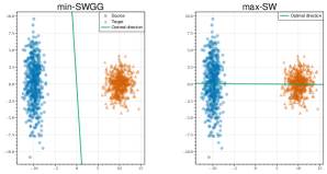
Refer to caption
Figure 6: Optimal θ𝜃\theta for max-SW and min-SWGG

A.5 From permutations to transport map

In this section we provide the way of having a transport map from permutations.

Let μ1,μ2𝒫2n(d)subscript𝜇1subscript𝜇2subscriptsuperscript𝒫𝑛2superscript𝑑\mu_{1},\mu_{2}\in\mathcal{P}^{n}_{2}(\mathbb{R}^{d}), let θargminSWGGsuperscript𝜃SWGG\theta^{*}\in\arg\min\textnormal{SWGG} and let σθ,τθsubscript𝜎superscript𝜃subscript𝜏superscript𝜃\sigma_{\theta^{*}},\tau_{\theta^{*}} the associated permutations. The associated map must be T(𝒙σ(i))=𝒚τ(i)1in𝑇subscript𝒙𝜎𝑖subscript𝒚𝜏𝑖for-all1𝑖𝑛T(\boldsymbol{x}_{\sigma(i)})=\boldsymbol{y}_{\tau(i)}\;\forall 1\leq i\leq n. In the paper, we formulate the associated transport map as:

T(𝒙i)=𝒚τθ1(σθ(i)),1in.formulae-sequence𝑇subscript𝒙𝑖subscript𝒚superscriptsubscript𝜏superscript𝜃1subscript𝜎superscript𝜃𝑖for-all1𝑖𝑛T(\boldsymbol{x}_{i})=\boldsymbol{y}_{\tau_{\theta^{*}}^{-1}(\sigma_{\theta^{*}}(i))},\quad\forall 1\leq i\leq n. (24)

Moreover, the matrix representation of T𝑇T is given by:

Tij={1n if σ(i)=τ(j)0 otherwise subscript𝑇𝑖𝑗cases1𝑛 if 𝜎𝑖𝜏𝑗0 otherwise \displaystyle T_{ij}=\left\{\begin{array}[]{cl}\frac{1}{n}&\text{ if }\sigma(i)=\tau(j)\\ 0&\text{ otherwise }\end{array}\right. (27)

A.6 Examples of Transport Plan

Fig. 7 illustrates two instances of the transport plan obtained via min-SWGG. Even though these transport plans are not optimal, they were able to capture the overall structure of the true optimal transport plans.
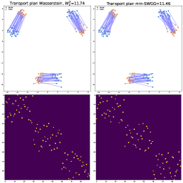
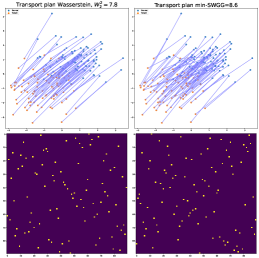
Refer to caption
Refer to caption
Figure 7: Example of transports plan given by Wasserstein (left and middle-right) and min-SWGG (middle left and right). Transport plan distribution (top) and transport matrix (bottom).The relative distances between source and target are given in the title.

The first example shows that the OT plan by min-SWGG exhibits a "block" structure, and thus approximates well the true Wasserstein distance. The second example shows that even in a context of superimposed distribution the "general transport direction" in min-SWGG is representative of that of the optimal transport map.

Appendix B Background on Wasserstein Generalized Geodesics

We introduce some concepts related the Wasserstein generalized geodesics in Sec. 4.1. In this section, we provide more details about these geodesics in order to provide a wider view on this theory.

In the following definitions, we do not address the issue of uniqueness of the geodesics. However this is not a problem in our setup since we focus our study on pivot measure with n𝑛n-atoms ν𝒫2n(d)𝜈subscriptsuperscript𝒫𝑛2superscript𝑑\nu\in\mathcal{P}^{n}_{2}(\mathbb{R}^{d}). In this case, we have uniqueness of the ν𝜈\nu-based Wasserstein distance [47].

Wasserstein generalized geodesics

As mentioned in Sec. 4.1, Wasserstein generalized geodesics rely on a pivot measure ν𝒫2n(d)𝜈subscriptsuperscript𝒫𝑛2superscript𝑑\nu\in\mathcal{P}^{n}_{2}(\mathbb{R}^{d}) to transport μ1subscript𝜇1\mu_{1} to μ2subscript𝜇2\mu_{2}. Indeed, one can leverage the optimal transport maps Tνμ1superscript𝑇𝜈subscript𝜇1T^{\nu\to\mu_{1}} and Tνμ2superscript𝑇𝜈subscript𝜇2T^{\nu\to\mu_{2}} to construct a curve linking μ1subscript𝜇1\mu_{1} to μ2subscript𝜇2\mu_{2}. The generalized geodesic with pivot measure ν𝜈\nu is defined as:

μg12(t)=def((1t)Tνμ1+tTνμ2)#νt[0,1].formulae-sequencesuperscriptdefsubscriptsuperscript𝜇12𝑔𝑡subscript1𝑡superscript𝑇𝜈subscript𝜇1𝑡superscript𝑇𝜈subscript𝜇2#𝜈for-all𝑡01\mu^{1\to 2}_{g}(t)\stackrel{{\scriptstyle\text{def}}}{{\,\,=\,}}\left((1-t)T^{\nu\to\mu_{1}}+tT^{\nu\to\mu_{2}}\right)_{\#}\nu\quad\quad\forall t\in[0,1]. (28)

The generalized Wasserstein mean refers to the middle of the geodesic, i.e. when t=0.5𝑡0.5t=0.5 and has been denoted μg12subscriptsuperscript𝜇12𝑔\mu^{1\to 2}_{g}.

Intuitively, the optimal transport maps between ν𝜈\nu and μi,i=1,2formulae-sequencesubscript𝜇𝑖𝑖12\mu_{i},i=1,2 give rise to a sub-optimal transport map between μ1subscript𝜇1\mu_{1} and μ2subscript𝜇2\mu_{2} through:

Tν12=defTνμ2Tμ1νwith(Tν12)#μ1=μ2.formulae-sequencesuperscriptdefsuperscriptsubscript𝑇𝜈12superscript𝑇𝜈subscript𝜇2superscript𝑇subscript𝜇1𝜈withsubscriptsuperscriptsubscript𝑇𝜈12#subscript𝜇1subscript𝜇2\displaystyle T_{\nu}^{1\to 2}\stackrel{{\scriptstyle\text{def}}}{{\,\,=\,}}T^{\nu\to\mu_{2}}\circ T^{\mu_{1}\to\nu}\quad\text{with}\quad(T_{\nu}^{1\to 2})_{\#}\mu_{1}=\mu_{2}. (29)

Tν12superscriptsubscript𝑇𝜈12T_{\nu}^{1\to 2} links μ1subscript𝜇1\mu_{1} to μ2subscript𝜇2\mu_{2} via the generalized geodesic:

μg12(t)=((1t)Id+tTν12)#μ1.subscriptsuperscript𝜇12𝑔𝑡subscript1𝑡𝐼𝑑𝑡superscriptsubscript𝑇𝜈12#subscript𝜇1\displaystyle\mu^{1\to 2}_{g}(t)=((1-t)Id+tT_{\nu}^{1\to 2})_{\#}\mu_{1}. (30)

We recall here the ν𝜈\nu-based Wasserstein distance induced by Tν12superscriptsubscript𝑇𝜈12T_{\nu}^{1\to 2} and introduced in Eq. (13).

Definition B.1.

The ν𝜈\nu-based Wasserstein distance [21, 47] is defined as:

Wν2(μ1,μ2)=defsuperscriptdefsubscriptsuperscript𝑊2𝜈subscript𝜇1subscript𝜇2absent\displaystyle W^{2}_{\nu}(\mu_{1},\mu_{2})\stackrel{{\scriptstyle\text{def}}}{{\,\,=\,}} d𝒙Tν12(𝒙)22𝑑μ1(𝒙)subscriptsuperscript𝑑subscriptsuperscriptnorm𝒙superscriptsubscript𝑇𝜈12𝒙22differential-dsubscript𝜇1𝒙\displaystyle\int_{\mathbb{R}^{d}}\|\boldsymbol{x}-T_{\nu}^{1\to 2}(\boldsymbol{x})\|^{2}_{2}d\mu_{1}(\boldsymbol{x}) (31)
=\displaystyle= dTνμ1(𝒛)Tνμ2(𝒛)22𝑑ν(𝒛).subscriptsuperscript𝑑subscriptsuperscriptnormsuperscript𝑇𝜈subscript𝜇1𝒛superscript𝑇𝜈subscript𝜇2𝒛22differential-d𝜈𝒛\displaystyle\int_{\mathbb{R}^{d}}\|T^{\nu\to\mu_{1}}(\boldsymbol{z})-T^{\nu\to\mu_{2}}(\boldsymbol{z})\|^{2}_{2}d\nu(\boldsymbol{z}). (32)

Moreover, this new notion of geodesics comes with an inequality, which is of the opposite side to Eq. (3):

W22(μg12(t),ν)subscriptsuperscript𝑊22subscriptsuperscript𝜇12𝑔𝑡𝜈\displaystyle W^{2}_{2}(\mu^{1\to 2}_{g}(t),\nu) (1t)W22(μ1,ν)+tW22(ν,μ2)t(1t)W22(μ1,μ2).absent1𝑡subscriptsuperscript𝑊22subscript𝜇1𝜈𝑡superscriptsubscript𝑊22𝜈subscript𝜇2𝑡1𝑡superscriptsubscript𝑊22subscript𝜇1subscript𝜇2\displaystyle\leq(1-t)W^{2}_{2}(\mu_{1},\nu)+tW_{2}^{2}(\nu,\mu_{2})-t(1-t)W_{2}^{2}(\mu_{1},\mu_{2}). (33)

The parallelogram law is not respected but straddles with eq. (3) and eq. (33). We refer to Figure 8 for an intuition behind positive curvature [51], parallelogram law and generalized geodesics.

μ1subscript𝜇1\mu_{1}μ1subscript𝜇1\mu_{1}ν𝜈\nuν𝜈\nuμ2subscript𝜇2\mu_{2}μ2subscript𝜇2\mu_{2}x1subscript𝑥1x_{1}y𝑦yx2subscript𝑥2x_{2}μ12(t)superscript𝜇12𝑡\mu^{1\ \rightarrow 2}(t)μg12(t)subscriptsuperscript𝜇12𝑔𝑡\mu^{1\rightarrow 2}_{g}(t)tx1+(1t)x2𝑡subscript𝑥11𝑡subscript𝑥2tx_{1}+(1-t)x_{2}
Figure 8: Geodesic (tId+(1t)T12)#μ1subscript𝑡𝐼𝑑1𝑡superscript𝑇12#subscript𝜇1(tId+(1-t)T^{1\to 2})_{\#}\mu_{1} and generalized geodesic (tId+(1t)Tν12)#μ1subscript𝑡𝐼𝑑1𝑡subscriptsuperscript𝑇12𝜈#subscript𝜇1(tId+(1-t)T^{1\to 2}_{\nu})_{\#}\mu_{1} in Wasserstein space (Left and Right) in dashed line and parallelogram law in dsuperscript𝑑\mathbb{R}^{d} (middle).

Setting t=0.5𝑡0.5t=0.5 in Eq. (33) and reordering the term gives:

W22(μ1,μ2)2W22(μ1,ν)+2W22(ν,μ2)4W22(μg12,ν).subscriptsuperscript𝑊22subscript𝜇1subscript𝜇22subscriptsuperscript𝑊22subscript𝜇1𝜈2subscriptsuperscript𝑊22𝜈subscript𝜇24subscriptsuperscript𝑊22subscriptsuperscript𝜇12𝑔𝜈\displaystyle W^{2}_{2}(\mu_{1},\mu_{2})\leq 2W^{2}_{2}(\mu_{1},\nu)+2W^{2}_{2}(\nu,\mu_{2})-4W^{2}_{2}(\mu^{1\to 2}_{g},\nu). (34)

Moreover one can remark that:

Wν2(μ1,μ2)=2W22(μ1,ν)+2W22(ν,μ2)4W22(μg12,ν)subscriptsuperscript𝑊2𝜈subscript𝜇1subscript𝜇22subscriptsuperscript𝑊22subscript𝜇1𝜈2subscriptsuperscript𝑊22𝜈subscript𝜇24subscriptsuperscript𝑊22subscriptsuperscript𝜇12𝑔𝜈\displaystyle W^{2}_{\nu}(\mu_{1},\mu_{2})=2W^{2}_{2}(\mu_{1},\nu)+2W^{2}_{2}(\nu,\mu_{2})-4W^{2}_{2}(\mu^{1\to 2}_{g},\nu) (35)

In particular situations Wν2superscriptsubscript𝑊𝜈2W_{\nu}^{2} and W22subscriptsuperscript𝑊22W^{2}_{2} coincide. It is the case for 1D distributions where the Wasserstein space is known to be flat [4]. In that case, the Wasserstein mean and the generalized Wasserstein mean are the same.

Multi-marginal

Another formulation of the ν𝜈\nu-based Wasserstein distance is possible through the perspective of multi-marginal OT [4]. Let Π(μ1,μ2,ν)={πs.t.P#12π=π12,P#13π=π1νandP#23π=π2ν}Πsubscript𝜇1subscript𝜇2𝜈formulae-sequence𝜋s.t.subscriptsuperscript𝑃12#𝜋superscript𝜋12subscriptsuperscript𝑃13#𝜋superscript𝜋1𝜈andsubscriptsuperscript𝑃23#𝜋superscript𝜋2𝜈\Pi(\mu_{1},\mu_{2},\nu)=\{\pi\;\text{s.t.}\;P^{12}_{\#}\pi=\pi^{1\to 2}\;,\;P^{13}_{\#}\pi=\pi^{1\to\nu}\;\text{and}\;P^{23}_{\#}\pi=\pi^{2\to\nu}\}, where Pijsuperscript𝑃𝑖𝑗P^{ij} is the projection onto the coordinates i,j𝑖𝑗i,j. Let also Π(μi,ν)superscriptΠsubscript𝜇𝑖𝜈\Pi^{*}(\mu_{i},\nu) be the space of optimal transport maps between μisubscript𝜇𝑖\mu_{i} and ν𝜈\nu. We have:

Wν2(μ1,μ2)=infπΠ(μ1,μ2,ν)s.t.P#i3πΠ(μi,ν)i=1,2d𝒙𝒚22𝑑π(𝒙,𝒚)superscriptsubscript𝑊𝜈2subscript𝜇1subscript𝜇2subscriptinfimumformulae-sequence𝜋Πsubscript𝜇1subscript𝜇2𝜈s.t.subscriptsuperscript𝑃𝑖3#𝜋superscriptΠsubscript𝜇𝑖𝜈𝑖12subscriptsuperscript𝑑subscriptsuperscriptnorm𝒙𝒚22differential-d𝜋𝒙𝒚\displaystyle W_{\nu}^{2}(\mu_{1},\mu_{2})=\inf_{\pi\in\Pi(\mu_{1},\mu_{2},\nu)\;\text{s.t.}\;P^{i3}_{\#}\pi\in\Pi^{*}(\mu_{i},\nu)\;i=1,2}\int_{\mathbb{R}^{d}}\|\boldsymbol{x}-\boldsymbol{y}\|^{2}_{2}d\pi(\boldsymbol{x},\boldsymbol{y}) (36)

Equation (36) expresses the fact that we select the optimal plan from Π(μ1,μ2,ν)Πsubscript𝜇1subscript𝜇2𝜈\Pi(\mu_{1},\mu_{2},\nu) which is already optimal for Π(μi,ν)Πsubscript𝜇𝑖𝜈\Pi(\mu_{i},\nu). Mathematically, this minimization is not a multi-marginal problem, since the optimal plan is supposed to be already optimal for some coordinate.

The set {πΠ(μ1,μ2,ν)s.t.P#i3πΠ(μi,ν)i=1,2}formulae-sequence𝜋Πsubscript𝜇1subscript𝜇2𝜈s.t.subscriptsuperscript𝑃𝑖3#𝜋superscriptΠsubscript𝜇𝑖𝜈𝑖12\{\pi\in\Pi(\mu_{1},\mu_{2},\nu)\;\text{s.t.}\;P^{i3}_{\#}\pi\in\Pi^{*}(\mu_{i},\nu)\;i=1,2\} is never empty, i.e. there is always existence of πν12superscriptsubscript𝜋𝜈12\pi_{\nu}^{1\to 2} (thanks to the gluing lemma [63], page 23). Moreover, in situations where it is a singleton, there is uniqueness of πν12subscriptsuperscript𝜋12𝜈\pi^{1\to 2}_{\nu}. Uniqueness is an ingredient which overpasses the selection of a final coupling and comes with additional result.

Lemma B.2 (Lemma 6 [47]).

Whenever {πΠ(μ1,μ2,ν)s.t.P#i3πΠ(μi,ν)i=1,2}formulae-sequence𝜋Πsubscript𝜇1subscript𝜇2𝜈s.t.subscriptsuperscript𝑃𝑖3#𝜋superscriptΠsubscript𝜇𝑖𝜈𝑖12\{\pi\in\Pi(\mu_{1},\mu_{2},\nu)\;\text{s.t.}\;P^{i3}_{\#}\pi\in\Pi^{*}(\mu_{i},\nu)\;i=1,2\} is a singleton, Wν2superscriptsubscript𝑊𝜈2W_{\nu}^{2} is a proper distance. It is a semi-distance otherwise.

Notably, 1D pivot measure was studied in [35] to ensure a dendritic structure of the distributions along the geodesic.

Appendix C Related Works

In this section we highlight the fact that several upper approximations of W22subscriptsuperscript𝑊22W^{2}_{2} are in the framework of generalized geodesics. The differences lay in the choice of the pivot measure ν𝜈\nu.

Factored Coupling.

In [29], the authors impose a low rank structure on the transport plan by factorizing the couplings through a pivot measure ν𝜈\nu expressed as the k𝑘k-Wasserstein mean between μ1subscript𝜇1\mu_{1} and μ2subscript𝜇2\mu_{2} (kn𝑘𝑛k\leq n). It is of particular interest since whenever the pivot distribution is the Wasserstein mean between μ1subscript𝜇1\mu_{1} and μ2subscript𝜇2\mu_{2}, Wν2superscriptsubscript𝑊𝜈2W_{\nu}^{2} and W22superscriptsubscript𝑊22W_{2}^{2} coincide.

Factored coupling results in a problem of computing the k𝑘k-Wasserstein mean (μ12superscript𝜇12\mu^{1\to 2}) followed by solving two OT problems between the clustered Wasserstein mean and the two input distributions (W22(μ1,μ12)superscriptsubscript𝑊22subscript𝜇1superscript𝜇12W_{2}^{2}(\mu_{1},\mu^{1\to 2}) and W22(μ12,μ2)subscriptsuperscript𝑊22superscript𝜇12subscript𝜇2W^{2}_{2}(\mu^{1\to 2},\mu_{2})). Even though the OT problems are smaller, they are still expensive in practice.

Moreover, in this scenario, the uniqueness of the OT plan Tν12subscriptsuperscript𝑇12𝜈T^{1\to 2}_{\nu} is not ensured. It appears that [29] chooses the most entropic transport plan, i.e. simply Tν12=Tμ12μ2Tμ1μ12subscriptsuperscript𝑇12𝜈superscript𝑇superscript𝜇12subscript𝜇2superscript𝑇subscript𝜇1superscript𝜇12T^{1\to 2}_{\nu}=T^{\mu^{1\to 2}\to\mu_{2}}\circ T^{\mu_{1}\to\mu^{1\to 2}}.

Subspace Detours.

From a statistical point of view, it is beneficial to consider optimal transport on a lower dimensional manifold [66]. In [44], authors compute an optimal transport plan Tμ1Eμ2Esuperscript𝑇subscriptsuperscript𝜇𝐸1subscriptsuperscript𝜇𝐸2T^{\mu^{E}_{1}\to\mu^{E}_{2}} between projections on a lower linear subspace E𝐸E of μ1subscript𝜇1\mu_{1} and μ2subscript𝜇2\mu_{2}, i.e. μiE=PE#μisuperscriptsubscript𝜇𝑖𝐸subscript𝑃𝐸#subscript𝜇𝑖\mu_{i}^{E}=P_{E}\#\mu_{i}, where PEsubscript𝑃𝐸P_{E} is the linear projection on E𝐸E. They aimed at leveraging Tμ1Eμ2Esuperscript𝑇superscriptsubscript𝜇1𝐸superscriptsubscript𝜇2𝐸T^{\mu_{1}^{E}\to\mu_{2}^{E}} to construct a sub-optimal map TE12superscriptsubscript𝑇𝐸12T_{E}^{1\to 2} between μ1subscript𝜇1\mu_{1} and μ2subscript𝜇2\mu_{2}.

The problem can be recast as a generalized geodesic problem with ν𝜈\nu being the Wasserstein mean of μ1Esuperscriptsubscript𝜇1𝐸\mu_{1}^{E} and μ2Esuperscriptsubscript𝜇2𝐸\mu_{2}^{E} embedded in dsuperscript𝑑\mathbb{R}^{d}. Once again, uniqueness of Tνμ1μ2superscriptsubscript𝑇𝜈subscript𝜇1subscript𝜇2T_{\nu}^{\mu_{1}\to\mu_{2}} is not guaranteed, authors provide two ways of selecting the map, namely Monge-Knothe and Monge-Independent lifting.

Subspace detours result in a problem where one needs to select a linear subspace E𝐸E (which is a non convex procedure), compute an optimal transport between μ1subscript𝜇1\mu_{1} and μ2subscript𝜇2\mu_{2} (in 𝒪(n3logn)𝒪superscript𝑛3𝑛\mathcal{O}(n^{3}\log n) whenever dim(E)>1dimension𝐸1\dim(E)>1) and reconstruct TEμ1μ2superscriptsubscript𝑇𝐸subscript𝜇1subscript𝜇2T_{E}^{\mu_{1}\to\mu_{2}}.

Linear Optimal Transport (LOT).

Given a set of distributions (μi)i=1m𝒫2(d)msuperscriptsubscriptsubscript𝜇𝑖𝑖1𝑚subscript𝒫2superscriptsuperscript𝑑𝑚(\mu_{i})_{i=1}^{m}\in\mathcal{P}_{2}(\mathbb{R}^{d})^{m}, LOT [65] embeds the set of distributions into the L2(ν)superscript𝐿2𝜈L^{2}(\nu)-space by computing the OT of each distribution to the pivot distribution. Mathematically, it computes Tνμi1imsuperscript𝑇𝜈subscript𝜇𝑖for-all1𝑖𝑚T^{\nu\to\mu_{i}}\;\forall 1\leq i\leq m and lies on estimating W22(μi,μj)superscriptsubscript𝑊22subscript𝜇𝑖subscript𝜇𝑗W_{2}^{2}(\mu_{i},\mu_{j}) with Wν2(μi,μj)superscriptsubscript𝑊𝜈2subscript𝜇𝑖subscript𝜇𝑗W_{\nu}^{2}(\mu_{i},\mu_{j}) through eq. (13).

In LOT, the pivot measure ν𝜈\nu was chosen to be the average of the input measures [65], the Lebesgue measure on dsuperscript𝑑\mathbb{R}^{d} [41] or an isotropic Gaussian distribution [43].

Instead of computing (m2)binomial𝑚2\binom{m}{2} expensive Wasserstein distances, it resorts only on m𝑚m Wasserstein distances between (μi)imsuperscriptsubscriptsubscript𝜇𝑖𝑖𝑚(\mu_{i})_{i}^{m} and ν𝜈\nu. While significantly reducing the computational cost when several distributions are at stake, it does not allow speeding up the computation when only two distributions are involved.

C.1 Linear Optimal Transport with shift and scaling

In this section, we recall the result from [43]. The theorem states that the ν𝜈\nu-based approximation is very close to WD whenever μ1subscript𝜇1\mu_{1}, μ2subscript𝜇2\mu_{2} are continuous distributions which are very close to be shift and scaling of each other. It can applies to a continuous version of SWGG, however it works with discrete measures in the particular case of equality between Wν2subscriptsuperscript𝑊2𝜈W^{2}_{\nu} and W22superscriptsubscript𝑊22W_{2}^{2}.

Theorem C.1 (Theorem 4.1 [43]).

Let Λ={Sa(shift),ad}{Rc(scaling),c}Λsubscript𝑆𝑎(shift)𝑎superscript𝑑subscript𝑅𝑐(scaling)𝑐\Lambda=\{S_{a}\;\text{(shift)}\;,a\in\mathbb{R}^{d}\}\cup\{R_{c}\;\text{(scaling)}\;,c\in\mathbb{R}\}, Λμ,R={hΛs.t.hμR}subscriptΛ𝜇𝑅conditional-setΛs.t.evaluated-at𝜇𝑅\Lambda_{\mu,R}=\{h\in\Lambda\;\text{s.t.}\;\|h\|_{\mu}\geq R\} and Gμ,R,ϵ={gL2(d,μ)s.t.hΛμ,Rs.t.ghμϵ}subscript𝐺𝜇𝑅italic-ϵconditional-set𝑔superscript𝐿2superscript𝑑𝜇s.t.subscriptΛ𝜇𝑅s.t.𝑔evaluated-at𝜇italic-ϵG_{\mu,R,\epsilon}=\{g\in L^{2}(\mathbb{R}^{d},\mu)\;\text{s.t.}\;\exists h\in\Lambda_{\mu,R}\;\text{s.t.}\;\|g-h\|_{\mu}\leq\epsilon\}

Let ν𝜈\nu, μ𝒫2(d)𝜇subscript𝒫2superscript𝑑\mu\in\mathcal{P}_{2}(\mathbb{R}^{d}), with μ,νλmuch-less-than𝜇𝜈𝜆\mu,\nu\ll\lambda (the Lebesgue measure). Let R>0,ϵ>0formulae-sequence𝑅0italic-ϵ0R>0,\epsilon>0

  • For g1,g2Gμ,R,ϵsubscript𝑔1subscript𝑔2subscript𝐺𝜇𝑅italic-ϵg_{1},g_{2}\in G_{\mu,R,\epsilon} and ν=λ𝜈𝜆\nu=\lambda on a convex compact subset of dsuperscript𝑑\mathbb{R}^{d}, we have:

    Wν(g1#μ,g2#μ)W2(g1#μ,g2#μ)Cϵ215+2ϵsubscript𝑊𝜈subscript𝑔1#𝜇subscript𝑔2#𝜇subscript𝑊2subscript𝑔1#𝜇subscript𝑔2#𝜇𝐶superscriptitalic-ϵ2152italic-ϵ\displaystyle W_{\nu}(g_{1\#}\mu,g_{2\#}\mu)-W_{2}(g_{1\#}\mu,g_{2\#}\mu)\leq C\epsilon^{\frac{2}{15}}+2\epsilon (37)
  • If μ𝜇\mu and ν𝜈\nu satisfy the assumption of Caffarelli’s regularity theorem [14], then for g1,g2Gμ,R,ϵsubscript𝑔1subscript𝑔2subscript𝐺𝜇𝑅italic-ϵg_{1},g_{2}\in G_{\mu,R,\epsilon}, we have:

    Wν(g1#μ,g2#μ)W2(g1#μ,g2#μ)C¯ϵ1/2+Cϵsubscript𝑊𝜈subscript𝑔1#𝜇subscript𝑔2#𝜇subscript𝑊2subscript𝑔1#𝜇subscript𝑔2#𝜇¯𝐶superscriptitalic-ϵ12𝐶italic-ϵ\displaystyle W_{\nu}(g_{1\#}\mu,g_{2\#}\mu)-W_{2}(g_{1\#}\mu,g_{2\#}\mu)\leq\overline{C}\epsilon^{1/2}+C\epsilon (38)

where C,C¯𝐶¯𝐶C,\overline{C} depdends on ν,μ𝜈𝜇\nu,\mu and R𝑅R.

Appendix D Proofs and other results related to Section 4

D.1 Proof of Proposition 4.2: equivalence between the two formulations of SWGG

In this section, we prove that the two definitions of SWGG in Def. 3.1 and Prop. 4.2 are equivalent. Let θ𝕊d1𝜃superscript𝕊𝑑1\theta\in\mathbb{S}^{d-1} be fixed.

From one side in Def. 3.1, we have:

SWGG22(μ1,μ2,θ)=def1ni𝒙σθ(i)𝒚τθ(i)22superscriptdefsuperscriptsubscriptSWGG22subscript𝜇1subscript𝜇2𝜃1𝑛subscript𝑖subscriptsuperscriptnormsubscript𝒙subscript𝜎𝜃𝑖subscript𝒚subscript𝜏𝜃𝑖22\displaystyle\textnormal{SWGG}_{2}^{2}(\mu_{1},\mu_{2},\theta)\stackrel{{\scriptstyle\text{def}}}{{\,\,=\,}}\frac{1}{n}\sum_{i}\|\boldsymbol{x}_{\sigma_{\theta}(i)}-\boldsymbol{y}_{\tau_{\theta}(i)}\|^{2}_{2} (39)

where σθsubscript𝜎𝜃\sigma_{\theta} and τθsubscript𝜏𝜃\tau_{\theta} are the permutations obtained by sorting P#θμ1subscriptsuperscript𝑃𝜃#subscript𝜇1P^{\theta}_{\#}\mu_{1} and P#θμ2subscriptsuperscript𝑃𝜃#subscript𝜇2P^{\theta}_{\#}\mu_{2}.

From the other side we note D(μ1,μ2,θ)𝐷subscript𝜇1subscript𝜇2𝜃D(\mu_{1},\mu_{2},\theta) the quantity:

D(μ1,μ2,θ)=def2W22(μ1,μθ12)+2W22(μθ12,μ2)4W22(μg,θ12,μθ12).superscriptdef𝐷subscript𝜇1subscript𝜇2𝜃2subscriptsuperscript𝑊22subscript𝜇1subscriptsuperscript𝜇12𝜃2superscriptsubscript𝑊22subscriptsuperscript𝜇12𝜃subscript𝜇24superscriptsubscript𝑊22subscriptsuperscript𝜇12𝑔𝜃subscriptsuperscript𝜇12𝜃\displaystyle D(\mu_{1},\mu_{2},\theta)\stackrel{{\scriptstyle\text{def}}}{{\,\,=\,}}2W^{2}_{2}(\mu_{1},\mu^{1\to 2}_{\theta})+2W_{2}^{2}(\mu^{1\to 2}_{\theta},\mu_{2})-4W_{2}^{2}(\mu^{1\to 2}_{g,\theta},\mu^{1\to 2}_{\theta}). (40)

We want to prove that SWGG22(μ1,μ2,θ)=D(μ1,μ2,θ),μ1,μ2𝒫2n(d)formulae-sequencesubscriptsuperscriptSWGG22subscript𝜇1subscript𝜇2𝜃𝐷subscript𝜇1subscript𝜇2𝜃for-allsubscript𝜇1subscript𝜇2subscriptsuperscript𝒫𝑛2superscript𝑑\textnormal{SWGG}^{2}_{2}(\mu_{1},\mu_{2},\theta)=D(\mu_{1},\mu_{2},\theta),\quad\forall\mu_{1},\mu_{2}\in\mathcal{P}^{n}_{2}(\mathbb{R}^{d}) and θ𝕊d1𝜃superscript𝕊𝑑1\theta\in\mathbb{S}^{d-1}.

Eq. (13) in the main paper states that D(μ1,μ2,θ)𝐷subscript𝜇1subscript𝜇2𝜃D(\mu_{1},\mu_{2},\theta) is equivalent to d𝒙Tμθ1212(𝒙)22𝑑μ1(𝒙)subscriptsuperscript𝑑subscriptsuperscriptnorm𝒙subscriptsuperscript𝑇12subscriptsuperscript𝜇12𝜃𝒙22differential-dsubscript𝜇1𝒙\int_{\mathbb{R}^{d}}\|\boldsymbol{x}-T^{1\to 2}_{\mu^{1\to 2}_{\theta}}(\boldsymbol{x})\|^{2}_{2}d\mu_{1}(\boldsymbol{x}).

Finally, Lemma 4.6 states that the transport map Tμθ1212subscriptsuperscript𝑇12subscriptsuperscript𝜇12𝜃T^{1\to 2}_{\mu^{1\to 2}_{\theta}} is fully determined by the permutations on the line: the projections part is a one-to-one correspondence between 𝒙𝒙\boldsymbol{x} and θ𝒙,θ𝜃𝒙𝜃\theta\langle\boldsymbol{x},\theta\rangle (resp. between 𝒚𝒚\boldsymbol{y} and θ𝒚,θ𝜃𝒚𝜃\theta\langle\boldsymbol{y},\theta\rangle). More formally Tμθ1212(𝒙σθ(i))=𝒚τθ(i)1informulae-sequencesubscriptsuperscript𝑇12subscriptsuperscript𝜇12𝜃subscript𝒙subscript𝜎𝜃𝑖subscript𝒚subscript𝜏𝜃𝑖for-all1𝑖𝑛T^{1\to 2}_{\mu^{1\to 2}_{\theta}}(\boldsymbol{x}_{\sigma_{\theta}(i)})=\boldsymbol{y}_{\tau_{\theta}(i)}\quad\forall 1\leq i\leq n. And thus we recover:

d𝒙Tμθ1212(𝒙)22𝑑μ1(𝒙)=1ni𝒙σθ(i)𝒚τθ(i)22subscriptsuperscript𝑑subscriptsuperscriptnorm𝒙subscriptsuperscript𝑇12subscriptsuperscript𝜇12𝜃𝒙22differential-dsubscript𝜇1𝒙1𝑛subscript𝑖subscriptsuperscriptnormsubscript𝒙subscript𝜎𝜃𝑖subscript𝒚subscript𝜏𝜃𝑖22\displaystyle\int_{\mathbb{R}^{d}}\|\boldsymbol{x}-T^{1\to 2}_{\mu^{1\to 2}_{\theta}}(\boldsymbol{x})\|^{2}_{2}d\mu_{1}(\boldsymbol{x})=\frac{1}{n}\sum_{i}\|\boldsymbol{x}_{\sigma_{\theta}(i)}-\boldsymbol{y}_{\tau_{\theta}(i)}\|^{2}_{2} (41)

which concludes the proof.

D.2 Proof of Weak Convergence (Proposition 4.3)

We want to prove that, for a sequence of measures (μk)k𝒫2n(d)subscriptsubscript𝜇𝑘𝑘subscriptsuperscript𝒫𝑛2superscript𝑑(\mu_{k})_{k\in\mathbb{N}}\in\mathcal{P}^{n}_{2}(\mathbb{R}^{d}), we have:

μk,2μ𝒫2n(d))min-SWGG22(μk,μ)𝑘0\displaystyle\mu_{k}\overset{\mathcal{L},2}{\longrightarrow}\mu\in\mathcal{P}^{n}_{2}(\mathbb{R}^{d}))\iff\textnormal{min-SWGG}_{2}^{2}(\mu_{k},\mu)\underset{k}{\longrightarrow}0 (42)

The notation μk,2μsubscript𝜇𝑘2𝜇\mu_{k}\overset{\mathcal{L},2}{\longrightarrow}\mu stands for the weak convergence in 𝒫2n(d)subscriptsuperscript𝒫𝑛2superscript𝑑\mathcal{P}^{n}_{2}(\mathbb{R}^{d}) i.e. df(𝒙)𝑑μ(k)(𝒙)df(𝒙)𝑑μ(𝒙)subscriptsuperscript𝑑𝑓𝒙differential-dsubscript𝜇𝑘𝒙subscriptsuperscript𝑑𝑓𝒙differential-d𝜇𝒙\int_{\mathbb{R}^{d}}f(\boldsymbol{x})d\mu_{(k)}(\boldsymbol{x})\to\int_{\mathbb{R}^{d}}f(\boldsymbol{x})d\mu(\boldsymbol{x}) for all continuous bounded functions f𝑓f and for the Euclidean distance f(𝒙)=𝒙0𝒙22𝑓𝒙superscriptsubscriptnormsubscript𝒙0𝒙22f(\boldsymbol{x})=\|\boldsymbol{x}_{0}-\boldsymbol{x}\|_{2}^{2} for all x0dsubscript𝑥0superscript𝑑x_{0}\in\mathbb{R}^{d}.

From one side, if min-SWGG22(μk,μ)0W22(μk,μ)0μk,2μsuperscriptsubscriptmin-SWGG22subscript𝜇𝑘𝜇0subscriptsuperscript𝑊22subscript𝜇𝑘𝜇0subscript𝜇𝑘2𝜇\textnormal{min-SWGG}_{2}^{2}(\mu_{k},\mu)\to 0\implies W^{2}_{2}(\mu_{k},\mu)\to 0\implies\mu_{k}\overset{\mathcal{L},2}{\longrightarrow}\mu. The first implication is due to the fact that min-SWGG22superscriptsubscriptmin-SWGG22\textnormal{min-SWGG}_{2}^{2} is an upper-bounds of W22subscriptsuperscript𝑊22W^{2}_{2}, the Wasserstein distance, and that WD metrizes the weak convergence.

From another side, assume μk,2μsubscript𝜇𝑘2𝜇\mu_{k}\overset{\mathcal{L},2}{\longrightarrow}\mu; we have for any θ𝜃\theta:

  1. 1.

    Let μθμkμ𝒫2n(d)superscriptsubscript𝜇𝜃subscript𝜇𝑘𝜇subscriptsuperscript𝒫𝑛2superscript𝑑\mu_{\theta}^{\mu_{k}\to\mu}\in\mathcal{P}^{n}_{2}(\mathbb{R}^{d}) stands for the Wasserstein mean of the projections Q#θμksubscriptsuperscript𝑄𝜃#subscript𝜇𝑘Q^{\theta}_{\#}\mu_{k} and Q#θμsubscriptsuperscript𝑄𝜃#𝜇Q^{\theta}_{\#}\mu and let μθμμ=Q#θμsuperscriptsubscript𝜇𝜃𝜇𝜇subscriptsuperscript𝑄𝜃#𝜇\mu_{\theta}^{\mu\to\mu}=Q^{\theta}_{\#}\mu. We have μθμkμsuperscriptsubscript𝜇𝜃subscript𝜇𝑘𝜇\mu_{\theta}^{\mu_{k}\to\mu} converges towards (in law) to μθμμsuperscriptsubscript𝜇𝜃𝜇𝜇\mu_{\theta}^{\mu\to\mu}, which implies that:

    W22(μk,μθμkμ)𝑘W22(μ,μθμμ).subscriptsuperscript𝑊22subscript𝜇𝑘superscriptsubscript𝜇𝜃subscript𝜇𝑘𝜇𝑘subscriptsuperscript𝑊22𝜇superscriptsubscript𝜇𝜃𝜇𝜇\displaystyle W^{2}_{2}(\mu_{k},\mu_{\theta}^{\mu_{k}\to\mu})\underset{k}{\longrightarrow}W^{2}_{2}(\mu,\mu_{\theta}^{\mu\to\mu}). (43)
  2. 2.

    Since μ𝒫2n(d)𝜇subscriptsuperscript𝒫𝑛2superscript𝑑\mu\in\mathcal{P}^{n}_{2}(\mathbb{R}^{d}), we have Tμθμkμμk𝑘Tμθμkμμsuperscript𝑇superscriptsubscript𝜇𝜃subscript𝜇𝑘𝜇subscript𝜇𝑘𝑘superscript𝑇superscriptsubscript𝜇𝜃subscript𝜇𝑘𝜇𝜇T^{\mu_{\theta}^{\mu_{k}\to\mu}\to\mu_{k}}\underset{k}{\longrightarrow}T^{\mu_{\theta}^{\mu_{k}\to\mu}\to\mu} (see [22], theorem 3.2). It implies that μg,θμkμμsuperscriptsubscript𝜇𝑔𝜃subscript𝜇𝑘𝜇𝜇\mu_{g,\theta}^{\mu_{k}\to\mu}\overset{\mathcal{L}}{\longrightarrow}\mu and particularly:

    W22(μg,θμkμ,μθμkμ)𝑘W22(μ,μθμμ)subscriptsuperscript𝑊22superscriptsubscript𝜇𝑔𝜃subscript𝜇𝑘𝜇superscriptsubscript𝜇𝜃subscript𝜇𝑘𝜇𝑘subscriptsuperscript𝑊22𝜇superscriptsubscript𝜇𝜃𝜇𝜇\displaystyle W^{2}_{2}(\mu_{g,\theta}^{\mu_{k}\to\mu},\mu_{\theta}^{\mu_{k}\to\mu})\underset{k}{\longrightarrow}W^{2}_{2}(\mu,\mu_{\theta}^{\mu\to\mu}) (44)

By combining the previous elements, we get:

2W22(μk,μθμkμ)+2W22(μθμkμ,μk)4W22(μg,θμkμ,μθμkμ)𝑘2subscriptsuperscript𝑊22subscript𝜇𝑘superscriptsubscript𝜇𝜃subscript𝜇𝑘𝜇2superscriptsubscript𝑊22superscriptsubscript𝜇𝜃subscript𝜇𝑘𝜇subscript𝜇𝑘4subscriptsuperscript𝑊22superscriptsubscript𝜇𝑔𝜃subscript𝜇𝑘𝜇superscriptsubscript𝜇𝜃subscript𝜇𝑘𝜇𝑘\displaystyle 2W^{2}_{2}(\mu_{k},\mu_{\theta}^{\mu_{k}\to\mu})+2W_{2}^{2}(\mu_{\theta}^{\mu_{k}\to\mu},\mu_{k})-4W^{2}_{2}(\mu_{g,\theta}^{\mu_{k}\to\mu},\mu_{\theta}^{\mu_{k}\to\mu})\underset{k}{\longrightarrow} 2W22(μ,μθμμ)2subscriptsuperscript𝑊22𝜇superscriptsubscript𝜇𝜃𝜇𝜇\displaystyle 2W^{2}_{2}(\mu,\mu_{\theta}^{\mu\to\mu})
+2W22(μθμμ,μ)2subscriptsuperscript𝑊22superscriptsubscript𝜇𝜃𝜇𝜇𝜇\displaystyle+2W^{2}_{2}(\mu_{\theta}^{\mu\to\mu},\mu)
4W22(μ,μθμμ)=04subscriptsuperscript𝑊22𝜇superscriptsubscript𝜇𝜃𝜇𝜇0\displaystyle-4W^{2}_{2}(\mu,\mu_{\theta}^{\mu\to\mu})=0 (45)

The previous relation shows that μk,2μsubscript𝜇𝑘2𝜇\mu_{k}\overset{\mathcal{L},2}{\longrightarrow}\mu implies SWGG22(μk,μ,θ)𝑘0subscriptsuperscriptSWGG22subscript𝜇𝑘𝜇𝜃𝑘0\textnormal{SWGG}^{2}_{2}(\mu_{k},\mu,\theta)\underset{k}{\longrightarrow}0 for any θ𝜃\theta. Hence, we can conclude that:

μk,2μmin-SWGG22(μk,μ)0subscript𝜇𝑘2𝜇superscriptsubscriptmin-SWGG22subscript𝜇𝑘𝜇0\displaystyle\mu_{k}\overset{\mathcal{L},2}{\longrightarrow}\mu\implies\textnormal{min-SWGG}_{2}^{2}(\mu_{k},\mu)\to 0 (46)

This concludes the proof.

Note that when μ1subscript𝜇1\mu_{1} and μ2subscript𝜇2\mu_{2} are continuous, [41] proved that when the distributions are smooth enough (i.e. respecting the Cafarelli theorem [14]), there is a bi-Holder equivalence between the ν𝜈\nu-based Wasserstein distance and W22subscriptsuperscript𝑊22W^{2}_{2}. Hence, it still holds for SWGG for any θSd1𝜃superscript𝑆𝑑1\theta\in S^{d-1}:

W22(μ1,μ2)SWGG22(μ1,μ2,θ)B×W22(μ1,μ2)2/15μi𝒫2(d)formulae-sequencesubscriptsuperscript𝑊22subscript𝜇1subscript𝜇2superscriptsubscriptSWGG22subscript𝜇1subscript𝜇2𝜃𝐵subscriptsuperscript𝑊22superscriptsubscript𝜇1subscript𝜇2215for-allsubscript𝜇𝑖subscript𝒫2superscript𝑑\displaystyle W^{2}_{2}(\mu_{1},\mu_{2})\leq\textnormal{SWGG}_{2}^{2}(\mu_{1},\mu_{2},\theta)\leq B\times W^{2}_{2}(\mu_{1},\mu_{2})^{2/15}\quad\quad\forall\mu_{i}\in\mathcal{P}_{2}(\mathbb{R}^{d}) (47)

where B𝐵B depends on μi,i{1,2},θformulae-sequencesubscript𝜇𝑖𝑖12𝜃\mu_{i},i\in\{1,2\},\theta and the dimension d𝑑d. This bound is sufficient to prove that SWGG metrizes the weak convergence in this context. We refer to [41] for more details.

D.3 Proof of Translation property (Proposition 4.4)

We prove that min-SWGG22subscriptsuperscriptmin-SWGG22\textnormal{min-SWGG}^{2}_{2} has the same behavior w.r.t. the translation as W22subscriptsuperscript𝑊22W^{2}_{2}. This property is well known for Wasserstein and useful in applications such as shape matching.

Let μ1,μ2𝒫2n(d)subscript𝜇1subscript𝜇2subscriptsuperscript𝒫𝑛2superscript𝑑\mu_{1},\mu_{2}\in\mathcal{P}^{n}_{2}(\mathbb{R}^{d}), and let Tusuperscript𝑇𝑢T^{u} (resp. Tvsuperscript𝑇𝑣T^{v}) be the map 𝒙𝒙𝒖maps-to𝒙𝒙𝒖\boldsymbol{x}\mapsto\boldsymbol{x}-\boldsymbol{u} (resp. 𝒙𝒙𝒗maps-to𝒙𝒙𝒗\boldsymbol{x}\mapsto\boldsymbol{x}-\boldsymbol{v}), with 𝒖,𝒗𝒖𝒗\boldsymbol{u},\boldsymbol{v} vectors of dsuperscript𝑑\mathbb{R}^{d}.

To ease the notations, let define μ~1=T#uμ1subscript~𝜇1subscriptsuperscript𝑇𝑢#subscript𝜇1\tilde{\mu}_{1}=T^{u}_{\#}\mu_{1} and μ~2=T#vμ2subscript~𝜇2subscriptsuperscript𝑇𝑣#subscript𝜇2\tilde{\mu}_{2}=T^{v}_{\#}\mu_{2}.

Let remind that in the case of Wasserstein distance we have [53](Remark 2.19):

W22(μ~1,μ~2)=defW22(T#uμ1,T#vμ2)=W22(μ1,μ2)2𝒖𝒗,𝒎1𝒎2+𝒖𝒗22superscriptdefsubscriptsuperscript𝑊22subscript~𝜇1subscript~𝜇2subscriptsuperscript𝑊22subscriptsuperscript𝑇𝑢#subscript𝜇1subscriptsuperscript𝑇𝑣#subscript𝜇2subscriptsuperscript𝑊22subscript𝜇1subscript𝜇22𝒖𝒗subscript𝒎1subscript𝒎2subscriptsuperscriptnorm𝒖𝒗22\displaystyle W^{2}_{2}(\tilde{\mu}_{1},\tilde{\mu}_{2})\stackrel{{\scriptstyle\text{def}}}{{\,\,=\,}}W^{2}_{2}(T^{u}_{\#}\mu_{1},T^{v}_{\#}\mu_{2})=W^{2}_{2}(\mu_{1},\mu_{2})-2\langle\boldsymbol{u}-\boldsymbol{v},\boldsymbol{m}_{1}-\boldsymbol{m}_{2}\rangle+\|\boldsymbol{u}-\boldsymbol{v}\|^{2}_{2} (48)

with 𝒎1=d𝒙𝑑μ1(𝒙)subscript𝒎1subscriptsuperscript𝑑𝒙differential-dsubscript𝜇1𝒙\boldsymbol{m}_{1}=\int_{\mathbb{R}^{d}}\boldsymbol{x}d\mu_{1}(\boldsymbol{x}) and 𝒎2=d𝒙𝑑μ2(𝒙)subscript𝒎2subscriptsuperscript𝑑𝒙differential-dsubscript𝜇2𝒙\boldsymbol{m}_{2}=\int_{\mathbb{R}^{d}}\boldsymbol{x}d\mu_{2}(\boldsymbol{x}).

We aim to compute min-SWGG22(μ~1,μ~2)=defmin-SWGG22(T#uμ1,T#vμ2)superscriptdefsubscriptsuperscriptmin-SWGG22subscript~𝜇1subscript~𝜇2subscriptsuperscriptmin-SWGG22subscriptsuperscript𝑇𝑢#subscript𝜇1subscriptsuperscript𝑇𝑣#subscript𝜇2\textnormal{min-SWGG}^{2}_{2}(\tilde{\mu}_{1},\tilde{\mu}_{2})\stackrel{{\scriptstyle\text{def}}}{{\,\,=\,}}\textnormal{min-SWGG}^{2}_{2}(T^{u}_{\#}\mu_{1},T^{v}_{\#}\mu_{2}). Let express first

SWGG22(μ~1,μ~2)subscriptsuperscriptSWGG22subscript~𝜇1subscript~𝜇2\displaystyle\textnormal{SWGG}^{2}_{2}(\tilde{\mu}_{1},\tilde{\mu}_{2}) =2W22(μ~1,μ~θ12)+2W22(μ~2,μ~θ12)4W22(μ~g,θ12,μ~θ12)absent2subscriptsuperscript𝑊22subscript~𝜇1subscriptsuperscript~𝜇12𝜃2subscriptsuperscript𝑊22subscript~𝜇2subscriptsuperscript~𝜇12𝜃4subscriptsuperscript𝑊22subscriptsuperscript~𝜇12𝑔𝜃subscriptsuperscript~𝜇12𝜃\displaystyle=2W^{2}_{2}(\tilde{\mu}_{1},\tilde{\mu}^{1\to 2}_{\theta})+2W^{2}_{2}(\tilde{\mu}_{2},\tilde{\mu}^{1\to 2}_{\theta})-4W^{2}_{2}(\tilde{\mu}^{1\to 2}_{g,\theta},\tilde{\mu}^{1\to 2}_{\theta}) (49)

where μ~θ12subscriptsuperscript~𝜇12𝜃\tilde{\mu}^{1\to 2}_{\theta} is the Wasserstein mean of the projections along θ𝜃\theta of the shifted measures μ~1=T#uμ1subscript~𝜇1subscriptsuperscript𝑇𝑢#subscript𝜇1\tilde{\mu}_{1}=T^{u}_{\#}\mu_{1} and μ~2=T#vμ2subscript~𝜇2subscriptsuperscript𝑇𝑣#subscript𝜇2\tilde{\mu}_{2}=T^{v}_{\#}\mu_{2} as in Proposition 2. The generalized Wasserstein mean μ~g,θ12subscriptsuperscript~𝜇12𝑔𝜃\tilde{\mu}^{1\to 2}_{g,\theta} is defined accordingly (see also Proposition 11).

We have:

W22(μ~1,μ~θ12)=W22(μ1,μθ12)2𝒖,𝒎1𝒎3+𝒖22subscriptsuperscript𝑊22subscript~𝜇1subscriptsuperscript~𝜇12𝜃subscriptsuperscript𝑊22subscript𝜇1subscriptsuperscript𝜇12𝜃2𝒖subscript𝒎1subscript𝒎3subscriptsuperscriptnorm𝒖22\displaystyle W^{2}_{2}(\tilde{\mu}_{1},\tilde{\mu}^{1\to 2}_{\theta})=W^{2}_{2}(\mu_{1},\mu^{1\to 2}_{\theta})-2\langle\boldsymbol{u},\boldsymbol{m}_{1}-\boldsymbol{m}_{3}\rangle+\|\boldsymbol{u}\|^{2}_{2} (50)

where 𝒎3=d𝒙𝑑μ~θ12(𝒙)subscript𝒎3subscriptsuperscript𝑑𝒙differential-dsubscriptsuperscript~𝜇12𝜃𝒙\boldsymbol{m}_{3}=\int_{\mathbb{R}^{d}}\boldsymbol{x}d\tilde{\mu}^{1\to 2}_{\theta}(\boldsymbol{x}).

Similarly W22(μ~2,μ~θ12)=W22(μ2,μθ12)2𝒗,𝒎2𝒎3+𝒗22subscriptsuperscript𝑊22subscript~𝜇2subscriptsuperscript~𝜇12𝜃subscriptsuperscript𝑊22subscript𝜇2subscriptsuperscript𝜇12𝜃2𝒗subscript𝒎2subscript𝒎3subscriptsuperscriptnorm𝒗22W^{2}_{2}(\tilde{\mu}_{2},\tilde{\mu}^{1\to 2}_{\theta})=W^{2}_{2}(\mu_{2},\mu^{1\to 2}_{\theta})-2\langle\boldsymbol{v},\boldsymbol{m}_{2}-\boldsymbol{m}_{3}\rangle+\|\boldsymbol{v}\|^{2}_{2}.

Let express now the third term in eq. (49). For that we require to define the generalized Wasserstein mean μ~g,θ12subscriptsuperscript~𝜇12𝑔𝜃\tilde{\mu}^{1\to 2}_{g,\theta} with pivot measure μ~θ12subscriptsuperscript~𝜇12𝜃\tilde{\mu}^{1\to 2}_{\theta}. By the virtue of eq. (11) in the main paper, we have:

μ~g,θ12subscriptsuperscript~𝜇12𝑔𝜃\displaystyle\tilde{\mu}^{1\to 2}_{g,\theta} =(12Tμ~θ12μ~1+12Tμ~θ12μ~2)#μ~θ12absentsubscript12superscript𝑇subscriptsuperscript~𝜇12𝜃subscript~𝜇112superscript𝑇subscriptsuperscript~𝜇12𝜃subscript~𝜇2#subscriptsuperscript~𝜇12𝜃\displaystyle=\left(\frac{1}{2}T^{\tilde{\mu}^{1\to 2}_{\theta}\to\tilde{\mu}_{1}}+\frac{1}{2}T^{\tilde{\mu}^{1\to 2}_{\theta}\to\tilde{\mu}_{2}}\right)_{\#}\tilde{\mu}^{1\to 2}_{\theta} (51)
=(12Tμθ12μ1+12Tμθ12μ2Tu+v2)#μ~θ12absentsubscript12superscript𝑇subscriptsuperscript𝜇12𝜃subscript𝜇112superscript𝑇subscriptsuperscript𝜇12𝜃subscript𝜇2superscript𝑇𝑢𝑣2#subscriptsuperscript~𝜇12𝜃\displaystyle=\left(\frac{1}{2}T^{{\mu}^{1\to 2}_{\theta}\to\mu_{1}}+\frac{1}{2}T^{{\mu}^{1\to 2}_{\theta}\to\mu_{2}}-T^{\frac{u+v}{2}}\right)_{\#}\tilde{\mu}^{1\to 2}_{\theta} (52)
=T#u+v2((12Tμθ12μ1+12Tμθ12μ2)#μθ12)absentsubscriptsuperscript𝑇𝑢𝑣2#subscript12superscript𝑇subscriptsuperscript𝜇12𝜃subscript𝜇112superscript𝑇subscriptsuperscript𝜇12𝜃subscript𝜇2#subscriptsuperscript𝜇12𝜃\displaystyle=T^{\frac{u+v}{2}}_{\#}\left(\left(\frac{1}{2}T^{{\mu}^{1\to 2}_{\theta}\to\mu_{1}}+\frac{1}{2}T^{{\mu}^{1\to 2}_{\theta}\to\mu_{2}}\right)_{\#}\mu^{1\to 2}_{\theta}\right) (53)

Hence, the third term in (49) is:

W22(μ~g,θ12,μ~θ12)=W22(μg,θ12,μθ12)2<𝒖+𝒗2,𝒎1+𝒎22𝒎3>+𝒖+𝒗222formulae-sequencesubscriptsuperscript𝑊22subscriptsuperscript~𝜇12𝑔𝜃subscriptsuperscript~𝜇12𝜃subscriptsuperscript𝑊22subscriptsuperscript𝜇12𝑔𝜃subscriptsuperscript𝜇12𝜃2𝒖𝒗2subscript𝒎1subscript𝒎22subscript𝒎3subscriptsuperscriptdelimited-∥∥𝒖𝒗222\displaystyle W^{2}_{2}(\tilde{\mu}^{1\to 2}_{g,\theta},\tilde{\mu}^{1\to 2}_{\theta})=W^{2}_{2}(\mu^{1\to 2}_{g,\theta},\mu^{1\to 2}_{\theta})-2\Bigl{<}\frac{\boldsymbol{u}+\boldsymbol{v}}{2},\frac{\boldsymbol{m}_{1}+\boldsymbol{m}_{2}}{2}-\boldsymbol{m}_{3}\Bigr{>}+\Bigl{\|}\frac{\boldsymbol{u}+\boldsymbol{v}}{2}\Bigr{\|}^{2}_{2} (54)

since the mean of a Wasserstein mean is the mean of m1subscript𝑚1m_{1}, m2subscript𝑚2m_{2}.

Putting all together, we have:

min-SWGG22(T#uμ1,T#vμ2)subscriptsuperscriptmin-SWGG22subscriptsuperscript𝑇𝑢#subscript𝜇1subscriptsuperscript𝑇𝑣#subscript𝜇2\displaystyle\textnormal{min-SWGG}^{2}_{2}(T^{u}_{\#}\mu_{1},T^{v}_{\#}\mu_{2}) =min-SWGG22(μ1,μ2)absentsubscriptsuperscriptmin-SWGG22subscript𝜇1subscript𝜇2\displaystyle=\textnormal{min-SWGG}^{2}_{2}(\mu_{1},\mu_{2}) \displaystyle- 4𝒖,𝒎1𝒎34𝒗,𝒎2𝒎34𝒖subscript𝒎1subscript𝒎34𝒗subscript𝒎2subscript𝒎3\displaystyle 4\langle\boldsymbol{u},\boldsymbol{m}_{1}-\boldsymbol{m}_{3}\rangle-4\langle\boldsymbol{v},\boldsymbol{m}_{2}-\boldsymbol{m}_{3}\rangle (55)
+8<𝒖+𝒗2,𝒎1+𝒎22𝒎3>\displaystyle+8\Bigl{<}\frac{\boldsymbol{u}+\boldsymbol{v}}{2},\frac{\boldsymbol{m}_{1}+\boldsymbol{m}_{2}}{2}-\boldsymbol{m}_{3}\Bigr{>}
+2𝒖22+2𝒗224𝒖+𝒗2222subscriptsuperscriptnorm𝒖222subscriptsuperscriptnorm𝒗224subscriptsuperscriptdelimited-∥∥𝒖𝒗222\displaystyle+2\|\boldsymbol{u}\|^{2}_{2}+2\|\boldsymbol{v}\|^{2}_{2}-4\Bigl{\|}\frac{\boldsymbol{u}+\boldsymbol{v}}{2}\Bigr{\|}^{2}_{2}
=min-SWGG22(μ1,μ2)absentsubscriptsuperscriptmin-SWGG22subscript𝜇1subscript𝜇2\displaystyle=\textnormal{min-SWGG}^{2}_{2}(\mu_{1},\mu_{2}) +\displaystyle+ 4𝒖+𝒗,𝒎34𝒖𝒗subscript𝒎3\displaystyle 4\langle\boldsymbol{u}+\boldsymbol{v},\boldsymbol{m}_{3}\rangle (56)
4𝒖+𝒗,𝒎34𝒖,𝒎14𝒗,𝒎24𝒖𝒗subscript𝒎34𝒖subscript𝒎14𝒗subscript𝒎2\displaystyle-4\langle\boldsymbol{u}+\boldsymbol{v},\boldsymbol{m}_{3}\rangle-4\langle\boldsymbol{u},\boldsymbol{m}_{1}\rangle-4\langle\boldsymbol{v},\boldsymbol{m}_{2}\rangle
+4𝒖+𝒗,𝒎1+𝒎2+𝒖𝒗224𝒖𝒗subscript𝒎1subscript𝒎2subscriptsuperscriptnorm𝒖𝒗22\displaystyle+4\langle\boldsymbol{u}+\boldsymbol{v},\boldsymbol{m}_{1}+\boldsymbol{m}_{2}\rangle+\|\boldsymbol{u}-\boldsymbol{v}\|^{2}_{2}
=min-SWGG22(μ1,μ2)absentsubscriptsuperscriptmin-SWGG22subscript𝜇1subscript𝜇2\displaystyle=\textnormal{min-SWGG}^{2}_{2}(\mu_{1},\mu_{2}) \displaystyle- 2𝒖,𝒎12𝒗,𝒎2+2𝒖,𝒎2+2𝒗,𝒎12𝒖subscript𝒎12𝒗subscript𝒎22𝒖subscript𝒎22𝒗subscript𝒎1\displaystyle 2\langle\boldsymbol{u},\boldsymbol{m}_{1}\rangle-2\langle\boldsymbol{v},\boldsymbol{m}_{2}\rangle+2\langle\boldsymbol{u},\boldsymbol{m}_{2}\rangle+2\langle\boldsymbol{v},\boldsymbol{m}_{1}\rangle (57)
+𝒖𝒗22subscriptsuperscriptnorm𝒖𝒗22\displaystyle+\|\boldsymbol{u}-\boldsymbol{v}\|^{2}_{2}
=min-SWGG22(μ1,μ2)absentsubscriptsuperscriptmin-SWGG22subscript𝜇1subscript𝜇2\displaystyle=\textnormal{min-SWGG}^{2}_{2}(\mu_{1},\mu_{2}) \displaystyle- 2𝒖𝒗,𝒎1𝒎2+𝒖𝒗222𝒖𝒗subscript𝒎1subscript𝒎2subscriptsuperscriptnorm𝒖𝒗22\displaystyle 2\langle\boldsymbol{u}-\boldsymbol{v},\boldsymbol{m}_{1}-\boldsymbol{m}_{2}\rangle+\|\boldsymbol{u}-\boldsymbol{v}\|^{2}_{2} (58)

D.4 Proof of the new closed form of the Wasserstein distance (Lemma 4.6)

We recall and prove the lemma that makes explicit a new closed form for WD. Let μ1,μ2subscript𝜇1subscript𝜇2\mu_{1},\mu_{2} be in 𝒫2n(d)subscriptsuperscript𝒫𝑛2superscript𝑑\mathcal{P}^{n}_{2}(\mathbb{R}^{d}) with μ2subscript𝜇2\mu_{2} a distribution supported on a line whose direction is θ𝕊d1𝜃superscript𝕊𝑑1\theta\in\mathbb{S}^{d-1}. We have:

W22(μ1,μ2)=W22(μ1,Q#θμ1)+W22(Q#θμ1,μ2).subscriptsuperscript𝑊22subscript𝜇1subscript𝜇2subscriptsuperscript𝑊22subscript𝜇1superscriptsubscript𝑄#𝜃subscript𝜇1subscriptsuperscript𝑊22superscriptsubscript𝑄#𝜃subscript𝜇1subscript𝜇2\displaystyle W^{2}_{2}(\mu_{1},\mu_{2})=W^{2}_{2}(\mu_{1},Q_{\#}^{\theta}\mu_{1})+W^{2}_{2}(Q_{\#}^{\theta}\mu_{1},\mu_{2}). (59)

Moreover, the optimal map is given by T12=TQ#θμ1μ2Tμ1Q#θμ1=TQ#θμ1μ2Qθsuperscript𝑇12superscript𝑇subscriptsuperscript𝑄𝜃#subscript𝜇1subscript𝜇2superscript𝑇subscript𝜇1subscriptsuperscript𝑄𝜃#subscript𝜇1superscript𝑇subscriptsuperscript𝑄𝜃#subscript𝜇1subscript𝜇2superscript𝑄𝜃T^{1\to 2}=T^{Q^{\theta}_{\#}\mu_{1}\to\mu_{2}}\circ T^{\mu_{1}\to Q^{\theta}_{\#}\mu_{1}}=T^{Q^{\theta}_{\#}\mu_{1}\to\mu_{2}}\circ Q^{\theta}.

Let μ1,μ2subscript𝜇1subscript𝜇2\mu_{1},\mu_{2} be in 𝒫2n(d)subscriptsuperscript𝒫𝑛2superscript𝑑\mathcal{P}^{n}_{2}(\mathbb{R}^{d}) with μ2subscript𝜇2\mu_{2} a distribution supported on a line of direction θ𝜃\theta. We have:

W22(μ1,μ2)=W22(μ1,Q#θμ1)+W22(Q#θμ1,μ2)subscriptsuperscript𝑊22subscript𝜇1subscript𝜇2subscriptsuperscript𝑊22subscript𝜇1superscriptsubscript𝑄#𝜃subscript𝜇1subscriptsuperscript𝑊22superscriptsubscript𝑄#𝜃subscript𝜇1subscript𝜇2\displaystyle W^{2}_{2}(\mu_{1},\mu_{2})=W^{2}_{2}(\mu_{1},Q_{\#}^{\theta}\mu_{1})+W^{2}_{2}(Q_{\#}^{\theta}\mu_{1},\mu_{2}) (60)

Moreover, the optimal map is given by:

T12=TQ#θμ12T1Q#θμ1=TQ#θμ12Qθsuperscript𝑇12superscript𝑇subscriptsuperscript𝑄𝜃#subscript𝜇12superscript𝑇1subscriptsuperscript𝑄𝜃#subscript𝜇1superscript𝑇subscriptsuperscript𝑄𝜃#subscript𝜇12superscript𝑄𝜃\displaystyle T^{1\to 2}=T^{Q^{\theta}_{\#}\mu_{1}\to 2}\circ T^{1\to Q^{\theta}_{\#}\mu_{1}}=T^{Q^{\theta}_{\#}\mu_{1}\to 2}\circ Q^{\theta} (61)

Here Qθsuperscript𝑄𝜃Q^{\theta} is given in Def. 4.1 of the paper.

The proof of the Lemma was first inspired by [13](Proposition 2.3), where authors show that WC2(μ1,μ2)=WC12(μ1,μ)+WC22(μ,μ2)subscriptsuperscript𝑊2𝐶subscript𝜇1subscript𝜇2subscriptsuperscript𝑊2superscript𝐶1subscript𝜇1𝜇subscriptsuperscript𝑊2superscript𝐶2𝜇subscript𝜇2W^{2}_{C}(\mu_{1},\mu_{2})=W^{2}_{C^{1}}(\mu_{1},\mu)+W^{2}_{C^{2}}(\mu,\mu_{2}) , with C1,C2superscript𝐶1superscript𝐶2C^{1},C^{2} and C𝐶C some cost matrices with the constraints Cij=minsCis1+Csj2subscript𝐶𝑖𝑗subscript𝑠subscriptsuperscript𝐶1𝑖𝑠subscriptsuperscript𝐶2𝑠𝑗C_{ij}=\min_{s}C^{1}_{is}+C^{2}_{sj}.

Let μ1=1nδ𝒙isubscript𝜇11𝑛subscript𝛿subscript𝒙𝑖\mu_{1}=\frac{1}{n}\sum\delta_{\boldsymbol{x}_{i}} and μ2=1nδ𝒚¯isubscript𝜇21𝑛subscript𝛿subscript¯𝒚𝑖\mu_{2}=\frac{1}{n}\delta_{\overline{\boldsymbol{y}}_{i}} be in 𝒫2n(d)subscriptsuperscript𝒫𝑛2superscript𝑑\mathcal{P}^{n}_{2}(\mathbb{R}^{d}) with μ2subscript𝜇2\mu_{2} a distribution supported on a line with direction θ𝜃\theta. Let Q#θμ1=μ¯1=1nδ𝒙¯i𝒫2n(d)superscriptsubscript𝑄#𝜃subscript𝜇1subscript¯𝜇11𝑛subscript𝛿subscript¯𝒙𝑖subscriptsuperscript𝒫𝑛2superscript𝑑Q_{\#}^{\theta}\mu_{1}=\overline{\mu}_{1}=\frac{1}{n}\sum\delta_{\overline{\boldsymbol{x}}_{i}}\in\mathcal{P}^{n}_{2}(\mathbb{R}^{d}). We emphasize here the fact that the atoms of μ¯1subscript¯𝜇1\overline{\mu}_{1} and μ2subscript𝜇2\mu_{2} are supported on a line are denoted by the overline symbol.

From one side, we have:

W22(μ1,μ2)subscriptsuperscript𝑊22subscript𝜇1subscript𝜇2\displaystyle W^{2}_{2}(\mu_{1},\mu_{2}) =infT1s.t.T#1μ1=μ2d𝒙T1(𝒙)22𝑑μ1(𝒙)absentsubscriptinfimumsuperscript𝑇1s.t.subscriptsuperscript𝑇1#subscript𝜇1subscript𝜇2subscriptsuperscript𝑑subscriptsuperscriptnorm𝒙superscript𝑇1𝒙22differential-dsubscript𝜇1𝒙\displaystyle=\inf_{T^{1}\;\text{s.t.}\;T^{1}_{\#}\mu_{1}=\mu_{2}}\int_{\mathbb{R}^{d}}\|\boldsymbol{x}-T^{1}(\boldsymbol{x})\|^{2}_{2}d\mu_{1}(\boldsymbol{x}) (62)
=infT1s.t.T#1μ1=μ2d(𝒙Qθ(𝒙)22+Qθ(𝒙)T1(𝒙)22)𝑑μ1(𝒙)absentsubscriptinfimumsuperscript𝑇1s.t.subscriptsuperscript𝑇1#subscript𝜇1subscript𝜇2subscriptsuperscript𝑑subscriptsuperscriptnorm𝒙superscript𝑄𝜃𝒙22subscriptsuperscriptnormsuperscript𝑄𝜃𝒙superscript𝑇1𝒙22differential-dsubscript𝜇1𝒙\displaystyle=\inf_{T^{1}\;\text{s.t.}\;T^{1}_{\#}\mu_{1}=\mu_{2}}\int_{\mathbb{R}^{d}}(\|\boldsymbol{x}-Q^{\theta}(\boldsymbol{x})\|^{2}_{2}+\|Q^{\theta}(\boldsymbol{x})-T^{1}(\boldsymbol{x})\|^{2}_{2}{{\color[rgb]{.75,0,.25}\definecolor[named]{pgfstrokecolor}{rgb}{.75,0,.25})}}d\mu_{1}(\boldsymbol{x}) (63)
=d𝒙Qθ(𝒙)22𝑑μ1(𝒙)+infT1s.t.T#1μ1=μ2dQθ(𝒙)T1(𝒙)22𝑑μ1(𝒙)absentsubscriptsuperscript𝑑subscriptsuperscriptnorm𝒙superscript𝑄𝜃𝒙22differential-dsubscript𝜇1𝒙subscriptinfimumsuperscript𝑇1s.t.subscriptsuperscript𝑇1#subscript𝜇1subscript𝜇2subscriptsuperscript𝑑subscriptsuperscriptnormsuperscript𝑄𝜃𝒙superscript𝑇1𝒙22differential-dsubscript𝜇1𝒙\displaystyle=\int_{\mathbb{R}^{d}}\|\boldsymbol{x}-Q^{\theta}(\boldsymbol{x})\|^{2}_{2}d\mu_{1}(\boldsymbol{x})+\inf_{T^{1}\;\text{s.t.}\;T^{1}_{\#}\mu_{1}=\mu_{2}}\int_{\mathbb{R}^{d}}\|Q^{\theta}(\boldsymbol{x})-T^{1}(\boldsymbol{x})\|^{2}_{2}d\mu_{1}(\boldsymbol{x}) (64)
infT2s.t.T#2μ1=μ¯1d𝒙T2(𝒙)22𝑑μ1(𝒙)+infT3s.t.T#3μ¯1=μ2d𝒙¯T3(𝒙¯)22𝑑μ¯1(𝒙¯)absentsubscriptinfimumsuperscript𝑇2s.t.subscriptsuperscript𝑇2#subscript𝜇1subscript¯𝜇1subscriptsuperscript𝑑subscriptsuperscriptnorm𝒙superscript𝑇2𝒙22differential-dsubscript𝜇1𝒙subscriptinfimumsuperscript𝑇3s.t.subscriptsuperscript𝑇3#subscript¯𝜇1subscript𝜇2subscriptsuperscript𝑑subscriptsuperscriptnorm¯𝒙superscript𝑇3¯𝒙22differential-dsubscript¯𝜇1¯𝒙\displaystyle\geq\inf_{T^{2}\;\text{s.t.}\;T^{2}_{\#}\mu_{1}=\overline{\mu}_{1}}\int_{\mathbb{R}^{d}}\|\boldsymbol{x}-T^{2}(\boldsymbol{x})\|^{2}_{2}d\mu_{1}(\boldsymbol{x})+\inf_{T^{3}\;\text{s.t.}\;T^{3}_{\#}\overline{\mu}_{1}=\mu_{2}}\int_{\mathbb{R}^{d}}\|\overline{\boldsymbol{x}}-T^{3}(\overline{\boldsymbol{x}})\|^{2}_{2}d\overline{\mu}_{1}(\overline{\boldsymbol{x}}) (65)
W22(μ1,μ¯1)+W22(μ¯1,μ2)absentsubscriptsuperscript𝑊22subscript𝜇1subscript¯𝜇1subscriptsuperscript𝑊22subscript¯𝜇1subscript𝜇2\displaystyle\geq W^{2}_{2}(\mu_{1},\overline{\mu}_{1})+W^{2}_{2}(\overline{\mu}_{1},\mu_{2}) (66)

Equation (63) is obtained thanks to the Pythagorean theorem since 𝒙i,Qθ(𝒙i),𝒚i¯subscript𝒙𝑖superscript𝑄𝜃subscript𝒙𝑖¯subscript𝒚𝑖\langle\boldsymbol{x}_{i},Q^{\theta}(\boldsymbol{x}_{i}),\overline{\boldsymbol{y}_{i}}\rangle is a right triangle 1infor-all1𝑖𝑛\forall 1\leq i\leq n. The equation (66) is obtained by taking the infinfimum\inf of the previous first term of the previous equation.

From the other side:

W22(μ1,μ¯1)+W22(μ¯1,μ2)=subscriptsuperscript𝑊22subscript𝜇1subscript¯𝜇1subscriptsuperscript𝑊22subscript¯𝜇1subscript𝜇2absent\displaystyle W^{2}_{2}(\mu_{1},\overline{\mu}_{1})+W^{2}_{2}(\overline{\mu}_{1},\mu_{2})= d𝒙¯T3(𝒙¯)22𝑑μ¯1(𝒙¯)+d𝒙¯T4(𝒙¯)22𝑑μ¯1(𝒙¯)subscriptsuperscript𝑑subscriptsuperscriptnorm¯𝒙superscript𝑇3¯𝒙22differential-dsubscript¯𝜇1¯𝒙subscriptsuperscript𝑑subscriptsuperscriptnorm¯𝒙superscript𝑇4¯𝒙22differential-dsubscript¯𝜇1¯𝒙\displaystyle\int_{\mathbb{R}^{d}}\|\overline{\boldsymbol{x}}-T^{3}(\overline{\boldsymbol{x}})\|^{2}_{2}d\overline{\mu}_{1}(\overline{\boldsymbol{x}})+\int_{\mathbb{R}^{d}}\|\overline{\boldsymbol{x}}-T^{4}(\overline{\boldsymbol{x}})\|^{2}_{2}d\overline{\mu}_{1}(\overline{\boldsymbol{x}}) (67)
=\displaystyle= dT3(𝒙¯)T4(𝒙¯)22𝑑μ¯1(𝒙¯)subscriptsuperscript𝑑subscriptsuperscriptnormsuperscript𝑇3¯𝒙superscript𝑇4¯𝒙22differential-dsubscript¯𝜇1¯𝒙\displaystyle\int_{\mathbb{R}^{d}}\|T^{3}(\overline{\boldsymbol{x}})-T^{4}(\overline{\boldsymbol{x}})\|^{2}_{2}d\overline{\mu}_{1}(\overline{\boldsymbol{x}}) (68)
=\displaystyle= Wμ¯12(μ1,μ2)W22(μ1,μ2)subscriptsuperscript𝑊2subscript¯𝜇1subscript𝜇1subscript𝜇2subscriptsuperscript𝑊22subscript𝜇1subscript𝜇2\displaystyle W^{2}_{\overline{\mu}_{1}}(\mu_{1},\mu_{2})\geq W^{2}_{2}(\mu_{1},\mu_{2}) (69)

Where T3superscript𝑇3T^{3} and T4superscript𝑇4T^{4} are the optimal plan of W22(μ1,μ¯1)subscriptsuperscript𝑊22subscript𝜇1subscript¯𝜇1W^{2}_{2}(\mu_{1},\overline{\mu}_{1}) and+W22(μ¯1,μ2)subscriptsuperscript𝑊22subscript¯𝜇1subscript𝜇2+W^{2}_{2}(\overline{\mu}_{1},\mu_{2}). Similarly, (67) is obtained via the Pythagorean theorem. This concludes the proof.

We plot an illustration of the lemma in Figure 9.
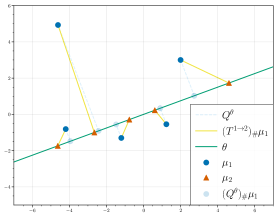
Refer to caption
Figure 9: Closed form for Wasserstein with Pythagorus theorem

D.5 Details on the efficient computation of SWGG

We decompose the second formulation of SWGG. Let first remind that Qθ:dd:superscript𝑄𝜃superscript𝑑superscript𝑑Q^{\theta}:\mathbb{R}^{d}\to\mathbb{R}^{d}, 𝒙θ𝒙,θmaps-to𝒙𝜃𝒙𝜃\boldsymbol{x}\mapsto\theta\langle\boldsymbol{x},\theta\rangle and Pθ:d:superscript𝑃𝜃superscript𝑑P^{\theta}:\mathbb{R}^{d}\to\mathbb{R}, 𝒙𝒙,θmaps-to𝒙𝒙𝜃\boldsymbol{x}\mapsto\langle\boldsymbol{x},\theta\rangle are the projections on the subspace generated by θ𝜃\theta.

We have:

SWGG22(μ1,μ2,θ)=2W22(μ1,μθ12)+2W22(μθ12,μ2)4W22(μg,θ12,μθ12).superscriptsubscriptSWGG22subscript𝜇1subscript𝜇2𝜃2subscriptsuperscript𝑊22subscript𝜇1subscriptsuperscript𝜇12𝜃2subscriptsuperscript𝑊22subscriptsuperscript𝜇12𝜃subscript𝜇24subscriptsuperscript𝑊22subscriptsuperscript𝜇12𝑔𝜃subscriptsuperscript𝜇12𝜃\displaystyle\textnormal{SWGG}_{2}^{2}(\mu_{1},\mu_{2},\theta)=2W^{2}_{2}(\mu_{1},\mu^{1\to 2}_{\theta})+2W^{2}_{2}(\mu^{1\to 2}_{\theta},\mu_{2})-4W^{2}_{2}(\mu^{1\to 2}_{g,\theta},\mu^{1\to 2}_{\theta}). (70)

First, by lemma 4.6,

2W22(μ1,μθ12)=2W22(μ1,Q#θμ1)+2W22(P#θμ1,P#θμθ12)2subscriptsuperscript𝑊22subscript𝜇1subscriptsuperscript𝜇12𝜃2subscriptsuperscript𝑊22subscript𝜇1subscriptsuperscript𝑄𝜃#subscript𝜇12subscriptsuperscript𝑊22subscriptsuperscript𝑃𝜃#subscript𝜇1subscriptsuperscript𝑃𝜃#subscriptsuperscript𝜇12𝜃\displaystyle 2W^{2}_{2}(\mu_{1},\mu^{1\to 2}_{\theta})=2W^{2}_{2}(\mu_{1},Q^{\theta}_{\#}\mu_{1})+2W^{2}_{2}(P^{\theta}_{\#}\mu_{1},P^{\theta}_{\#}\mu^{1\to 2}_{\theta}) (71)

as μθ12subscriptsuperscript𝜇12𝜃\mu^{1\to 2}_{\theta}’s support is on a line. Similarly,

2W22(μ2,μθ12)=2W22(μ2,Q#θμ2)+2W22(P#θμ2,P#θμθ12).2subscriptsuperscript𝑊22subscript𝜇2subscriptsuperscript𝜇12𝜃2subscriptsuperscript𝑊22subscript𝜇2subscriptsuperscript𝑄𝜃#subscript𝜇22subscriptsuperscript𝑊22subscriptsuperscript𝑃𝜃#subscript𝜇2subscriptsuperscript𝑃𝜃#subscriptsuperscript𝜇12𝜃\displaystyle 2W^{2}_{2}(\mu_{2},\mu^{1\to 2}_{\theta})=2W^{2}_{2}(\mu_{2},Q^{\theta}_{\#}\mu_{2})+2W^{2}_{2}(P^{\theta}_{\#}\mu_{2},P^{\theta}_{\#}\mu^{1\to 2}_{\theta}). (72)

and

4W22(μg,θ12,μθ12)=4W22(μg,θ12,Q#θμg,θ12)4W22(P#θμg,θ12,P#θμθ12).4subscriptsuperscript𝑊22subscriptsuperscript𝜇12𝑔𝜃subscriptsuperscript𝜇12𝜃4subscriptsuperscript𝑊22subscriptsuperscript𝜇12𝑔𝜃subscriptsuperscript𝑄𝜃#subscriptsuperscript𝜇12𝑔𝜃4subscriptsuperscript𝑊22subscriptsuperscript𝑃𝜃#subscriptsuperscript𝜇12𝑔𝜃subscriptsuperscript𝑃𝜃#subscriptsuperscript𝜇12𝜃\displaystyle-4W^{2}_{2}(\mu^{1\to 2}_{g,\theta},\mu^{1\to 2}_{\theta})=-4W^{2}_{2}(\mu^{1\to 2}_{g,\theta},Q^{\theta}_{\#}\mu^{1\to 2}_{g,\theta})-4W^{2}_{2}(P^{\theta}_{\#}\mu^{1\to 2}_{g,\theta},P^{\theta}_{\#}\mu^{1\to 2}_{\theta}). (73)

We notice that 2W22(P#θμ1,P#θμθ12)+2W22(P#θμθ12,P#θμ2)=W22(P#θμ1,P#θμ2)2subscriptsuperscript𝑊22subscriptsuperscript𝑃𝜃#subscript𝜇1subscriptsuperscript𝑃𝜃#subscriptsuperscript𝜇12𝜃2subscriptsuperscript𝑊22subscriptsuperscript𝑃𝜃#subscriptsuperscript𝜇12𝜃subscriptsuperscript𝑃𝜃#subscript𝜇2subscriptsuperscript𝑊22subscriptsuperscript𝑃𝜃#subscript𝜇1subscriptsuperscript𝑃𝜃#subscript𝜇22W^{2}_{2}(P^{\theta}_{\#}\mu_{1},P^{\theta}_{\#}\mu^{1\to 2}_{\theta})+2W^{2}_{2}(P^{\theta}_{\#}\mu^{1\to 2}_{\theta},P^{\theta}_{\#}\mu_{2})=W^{2}_{2}(P^{\theta}_{\#}\mu_{1},P^{\theta}_{\#}\mu_{2}) (as P#θμθ12subscriptsuperscript𝑃𝜃#subscriptsuperscript𝜇12𝜃P^{\theta}_{\#}\mu^{1\to 2}_{\theta} is the Wasserstein mean between P#θμ1subscriptsuperscript𝑃𝜃#subscript𝜇1P^{\theta}_{\#}\mu_{1} and P#θμ2subscriptsuperscript𝑃𝜃#subscript𝜇2P^{\theta}_{\#}\mu_{2}). We also notice that 4W22(P#θμg,θ12,P#θμθ12)=04subscriptsuperscript𝑊22subscriptsuperscript𝑃𝜃#subscriptsuperscript𝜇12𝑔𝜃subscriptsuperscript𝑃𝜃#subscriptsuperscript𝜇12𝜃0-4W^{2}_{2}(P^{\theta}_{\#}\mu^{1\to 2}_{g,\theta},P^{\theta}_{\#}\mu^{1\to 2}_{\theta})=0 (it comes from the fact that the generalized Wasserstein mean is induced by the permutations on the line), we can put all together to have:

SWGG22(μ1,μ2,θ)=2W22(μ1,Q#θμ1)+2W22(μ2,Q#θμ2)4W22(μg,θ12,Q#θμg,θ12)+W22(P#θμ1,P#θμ2)subscriptsuperscriptSWGG22subscript𝜇1subscript𝜇2𝜃2subscriptsuperscript𝑊22subscript𝜇1subscriptsuperscript𝑄𝜃#subscript𝜇12subscriptsuperscript𝑊22subscript𝜇2subscriptsuperscript𝑄𝜃#subscript𝜇24subscriptsuperscript𝑊22subscriptsuperscript𝜇12𝑔𝜃subscriptsuperscript𝑄𝜃#subscriptsuperscript𝜇12𝑔𝜃subscriptsuperscript𝑊22subscriptsuperscript𝑃𝜃#subscript𝜇1subscriptsuperscript𝑃𝜃#subscript𝜇2\displaystyle\textnormal{SWGG}^{2}_{2}(\mu_{1},\mu_{2},\theta)=2W^{2}_{2}(\mu_{1},Q^{\theta}_{\#}\mu_{1})+2W^{2}_{2}(\mu_{2},Q^{\theta}_{\#}\mu_{2})-4W^{2}_{2}(\mu^{1\to 2}_{g,\theta},Q^{\theta}_{\#}\mu^{1\to 2}_{g,\theta})+W^{2}_{2}(P^{\theta}_{\#}\mu_{1},P^{\theta}_{\#}\mu_{2}) (74)

One can show that SWGG is divided into 3 Wasserstein distances between a distribution and its projections on a line and 1D Wasserstein problem. This results in a very fast computation of SWGG.

D.6 Smoothing of SWGG

In this section, we give details on the smoothing procedure of min-SWGG, an additional landscape of SWGG and its smooth counterpart SWGG~~SWGG\widetilde{\textnormal{SWGG}} and an empirical heuristic for setting hyperparameters s𝑠s and ϵitalic-ϵ\epsilon.

Smoothing Procedure.

A natural surrogate would be to add an entropic regularization within the definition of Tμθ12μisuperscript𝑇subscriptsuperscript𝜇12𝜃subscript𝜇𝑖T^{\mu^{1\to 2}_{\theta}\to\mu_{i}}, i{1,2}𝑖12i\in\{1,2\} and to solve an additional optimal transport problem. Nevertheless, it would lead to an algorithm with an 𝒪(n2)𝒪superscript𝑛2\mathcal{O}(n^{2}) complexity. Instead, we build upon the blurred Wasserstein distance [26] between two distributions ν1subscript𝜈1\nu_{1} and ν2subscript𝜈2\nu_{2}:

Bϵ2(ν1,ν2)=defW22(kϵ/4ν1,kϵ/4ν2)superscriptdefsubscriptsuperscript𝐵2italic-ϵsubscript𝜈1subscript𝜈2superscriptsubscript𝑊22subscript𝑘italic-ϵ4subscript𝜈1subscript𝑘italic-ϵ4subscript𝜈2\displaystyle B^{2}_{\epsilon}({\nu}_{1},\nu_{2})\stackrel{{\scriptstyle\text{def}}}{{\,\,=\,}}W_{2}^{2}(k_{\epsilon/4}\ast{\nu}_{1},k_{\epsilon/4}\ast\nu_{2})

where \ast denotes the smoothing (convolution) operator and kϵ/4subscript𝑘italic-ϵ4k_{\epsilon/4} is the Gaussian kernel of deviation ϵ/2italic-ϵ2\sqrt{\epsilon}/2. In our case, it resorts in making s𝑠s copies of each sorted projections Pθ(𝒙i)superscript𝑃𝜃subscript𝒙𝑖P^{\theta}(\boldsymbol{x}_{i}) and Pθ(𝒚i)superscript𝑃𝜃subscript𝒚𝑖P^{\theta}(\boldsymbol{y}_{i}) respectively, to add a Gaussian noise of deviation ϵ/2italic-ϵ2\sqrt{\epsilon}/2 and to compute averages of sorted blurred copies 𝒙σsssubscriptsuperscript𝒙𝑠superscript𝜎𝑠\boldsymbol{x}^{s}_{\sigma^{s}}, 𝒚τsssubscriptsuperscript𝒚𝑠superscript𝜏𝑠\boldsymbol{y}^{s}_{\tau^{s}}:

(μθ12~)i=12sk=(i1)s+1is𝒙σs(k)s+𝒚τs(k)s.subscript~subscriptsuperscript𝜇12𝜃𝑖12𝑠superscriptsubscript𝑘𝑖1𝑠1𝑖𝑠subscriptsuperscript𝒙𝑠superscript𝜎𝑠𝑘subscriptsuperscript𝒚𝑠superscript𝜏𝑠𝑘(\widetilde{\mu^{1\to 2}_{\theta}})_{i}=\frac{1}{2s}\sum_{k=(i-1)s+1}^{is}\boldsymbol{x}^{s}_{\sigma^{s}(k)}+\boldsymbol{y}^{s}_{\tau^{s}(k)}. (75)

Further, we provide additional examples of the landscape of min-SWGG~(μ1,μ2)~min-SWGGsubscript𝜇1subscript𝜇2\widetilde{\textnormal{min-SWGG}}({\mu}_{1},{\mu}_{2}) and discuss how to choose empirically relevant s𝑠s and ϵitalic-ϵ\epsilon values.

[26] has shown that the blurred WD has the same asymptotic properties as the Sinkhorn divergence, with parameter ϵitalic-ϵ\epsilon the strength of the blurring: it interpolates between WD (when ϵ0italic-ϵ0\epsilon\to 0) and a degenerate constant value (when ϵitalic-ϵ\epsilon\to\infty).

To find a minimum of Eq. (16) in the paper (i.e. SWGG22~(μ1,μ2,θ)~superscriptsubscriptSWGG22subscript𝜇1subscript𝜇2𝜃\widetilde{\textnormal{SWGG}_{2}^{2}}({\mu}_{1},{\mu}_{2},\theta)), we iterate over:

θt+1=subscript𝜃𝑡1absent\displaystyle\theta_{t+1}= θt+ηθSWGG22~(μ1,μ2,θ)subscript𝜃𝑡𝜂subscript𝜃~subscriptsuperscriptSWGG22subscript𝜇1subscript𝜇2𝜃\displaystyle\theta_{t}+\eta\nabla_{\theta}\widetilde{\textnormal{SWGG}^{2}_{2}}(\mu_{1},\mu_{2},\theta)
θt+1=subscript𝜃𝑡1absent\displaystyle\theta_{t+1}= θt+1/θt+12subscript𝜃𝑡1subscriptnormsubscript𝜃𝑡12\displaystyle\theta_{t+1}/\|{\theta}_{t+1}\|_{2}

where η+𝜂subscript\eta\in\mathbb{R}_{+} is the learning rate. This procedure converges towards a local minima with a complexity of 𝒪(snd+snlog(sn))𝒪𝑠𝑛𝑑𝑠𝑛𝑠𝑛\mathcal{O}(snd+sn\log(sn)) for each iteration. Once the optimal direction θsuperscript𝜃\theta^{\star} is found, the final solution resorts to be the solution provided by SWGG22(μ1,μ2,θ)subscriptsuperscriptSWGG22subscript𝜇1subscript𝜇2superscript𝜃\textnormal{SWGG}^{2}_{2}(\mu_{1},\mu_{2},\theta^{\star}), where the induced optimal transport map is an unblurred matrix.

Heuristic for setting the hyperparameters of SWGG~~SWGG\widetilde{\textnormal{SWGG}}

We here provide an heuristic for setting parameters s𝑠s (number of copies of each points) and ϵitalic-ϵ\epsilon (strength of the blurring). We then give an example of the behavior of SWGG~~SWGG\widetilde{\textnormal{SWGG}} w.r.t. these hyper parameters.

Let μ1=1nδ𝒙isubscript𝜇11𝑛subscript𝛿subscript𝒙𝑖\mu_{1}=\frac{1}{n}\sum\delta_{\boldsymbol{x}_{i}} and μ2=1nδ𝒚isubscript𝜇21𝑛subscript𝛿subscript𝒚𝑖\mu_{2}=\frac{1}{n}\sum\delta_{\boldsymbol{y}_{i}}.

•  s+𝑠subscripts\in\mathbb{N}_{+} represents the number of copies of each sample. We observe empirically that the quantity sn𝑠𝑛sn should be large to provide a smooth landscape. It means that the s𝑠s values can be small when n𝑛n increases, allowing to keep a competitive algorithm (as the complexity depends on ns𝑛𝑠ns)

•  ϵ+italic-ϵsubscript\epsilon\in\mathbb{R}_{+} represents the variance of the blurred copies of each sample. Empirically, ϵitalic-ϵ\epsilon should depend on the variance of the distributions projected on the line. Indeed, an ϵitalic-ϵ\epsilon very close to zero will not smooth enough the discontinuities whereas a large ϵitalic-ϵ\epsilon will give a constant landscape.

As discussed in Section 4.3, finding an optimal θ𝕊d1𝜃superscript𝕊𝑑1\theta\in\mathbb{S}^{d-1} is a non convex problem and provides a discontinuous loss function. We give some examples of the landscape of SWGG~~SWGG\widetilde{\textnormal{SWGG}} w.r.t. different values of the hyperparameters in Fig. 10. The landscapes were computed with a set of projections θ𝜃\theta regularly sampled with angles [0,2π]absent02𝜋\in[0,2\pi].

We observe that the larger s𝑠s, the smoother SWGG~~SWGG\widetilde{\textnormal{SWGG}}. Additionally, raising ϵitalic-ϵ\epsilon tends to flatten SWGG~~SWGG\widetilde{\textnormal{SWGG}} w.r.t. θ𝜃\theta (erasing local minima). Indeed similarly to Sinkhorn, a large ϵitalic-ϵ\epsilon blurred the transport plan and thus homogenize all the value of SWGG w.r.t. θ𝜃\theta.

Moreover, we empirically observe that the number of samples for μ1subscript𝜇1\mu_{1} and μ2subscript𝜇2\mu_{2} enforces the continuity of SWGG. We then conjecture that the discontinuities of SWGG are due to artifact of the sampling and thus the smoothing operation erases this unwanted behavior. A full investigation of this assumption is left for future work.
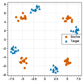
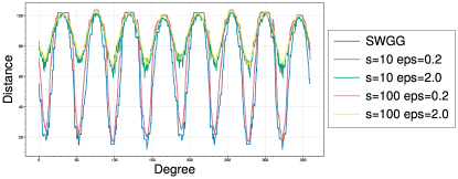
Refer to caption
Refer to caption
Refer to caption
Refer to caption
Figure 10: Non-convex landscapes for SWGG and SWGG~~SWGG\widetilde{\textnormal{SWGG}} with different hyper parameters.

D.7 Inconsequential of the pivot measure

Importantly, only the direction θ𝜃\theta is of importance for the value of SWGG. Indeed, whenever ν𝒫2n(d)𝜈subscriptsuperscript𝒫𝑛2superscript𝑑\nu\in\mathcal{P}^{n}_{2}(\mathbb{R}^{d}) is supported on a line of direction θ𝜃\theta, the position of the atoms is irrelevant for Wνsubscript𝑊𝜈W_{\nu} and the associated transport plan whenever the atoms are distinct. Despite the fact that the pivot measure is inconsequential for the value of SWGG (at θ𝜃\theta fixed), we choose it to be μθ12subscriptsuperscript𝜇12𝜃\mu^{1\to 2}_{\theta}. This choice is supported by the fact that μθ12subscriptsuperscript𝜇12𝜃\mu^{1\to 2}_{\theta} can be efficiently computed (as a 1D Wasserstein mean) and that some computation can be alleviated:

2W22(Q#θμ1,μθ12)+2W22(μθ12,Q#θμ2)=W22(Q#θμ1,Q#θμ2)2subscriptsuperscript𝑊22subscriptsuperscript𝑄𝜃#subscript𝜇1subscriptsuperscript𝜇12𝜃2subscriptsuperscript𝑊22subscriptsuperscript𝜇12𝜃subscriptsuperscript𝑄𝜃#subscript𝜇2subscriptsuperscript𝑊22subscriptsuperscript𝑄𝜃#subscript𝜇1subscriptsuperscript𝑄𝜃#subscript𝜇2\displaystyle 2W^{2}_{2}(Q^{\theta}_{\#}\mu_{1},\mu^{1\to 2}_{\theta})+2W^{2}_{2}(\mu^{1\to 2}_{\theta},Q^{\theta}_{\#}\mu_{2})=W^{2}_{2}(Q^{\theta}_{\#}\mu_{1},Q^{\theta}_{\#}\mu_{2}) (76)

It is an important comment to derive the property of distance for SWGG; it also allows minimizing SWGG over θ𝕊d1𝜃superscript𝕊𝑑1\theta\in\mathbb{S}^{d-1} without consideration for ν𝜈\nu, since any choice of ν𝜈\nu supported on the subspace generated by θ𝜃\theta give the same result for min-SWGG. This property of irrelevance comes from the nature of the subspace where ν𝜈\nu is supported, which is uni-dimensional. More formally we give the following proposition and its associated proof.

Proposition D.1.

Let μ1subscript𝜇1\mu_{1}, μ2𝒫2n(d)subscript𝜇2subscriptsuperscript𝒫𝑛2superscript𝑑\mu_{2}\in\mathcal{P}^{n}_{2}(\mathbb{R}^{d}). Let θ𝕊d1𝜃superscript𝕊𝑑1\theta\in\mathbb{S}^{d-1}. Let ν1,ν2𝒫2n(d)subscript𝜈1subscript𝜈2subscriptsuperscript𝒫𝑛2superscript𝑑\nu_{1},\nu_{2}\in\mathcal{P}^{n}_{2}(\mathbb{R}^{d}) be two pivot measures supported on a line with direction θ𝜃\theta, with disctincs atoms for each measure. We then have:

Wν12(μ1,μ2)=Wν22(μ1,μ2)subscriptsuperscript𝑊2subscript𝜈1subscript𝜇1subscript𝜇2subscriptsuperscript𝑊2subscript𝜈2subscript𝜇1subscript𝜇2\displaystyle W^{2}_{\nu_{1}}(\mu_{1},\mu_{2})=W^{2}_{\nu_{2}}(\mu_{1},\mu_{2}) (77)

We give a proof of this proposition.

Thanks to lemma 4.6, we known that the transport map Tν12superscriptsubscript𝑇𝜈12T_{\nu}^{1\to 2} is fully induced by the transport plan TνQ#θμ1Q#θμ2superscriptsubscript𝑇𝜈subscriptsuperscript𝑄𝜃#subscript𝜇1subscriptsuperscript𝑄𝜃#subscript𝜇2T_{\nu}^{Q^{\theta}_{\#}\mu_{1}\to Q^{\theta}_{\#}\mu_{2}}. Let remind that TνQ#θμ1Q#θμ2superscriptsubscript𝑇𝜈subscriptsuperscript𝑄𝜃#subscript𝜇1subscriptsuperscript𝑄𝜃#subscript𝜇2T_{\nu}^{Q^{\theta}_{\#}\mu_{1}\to Q^{\theta}_{\#}\mu_{2}} is given by TνQ#θμ2TQ#θμ1νsuperscript𝑇𝜈superscriptsubscript𝑄#𝜃subscript𝜇2superscript𝑇superscriptsubscript𝑄#𝜃subscript𝜇1𝜈T^{\nu\to Q_{\#}^{\theta}\mu_{2}}\circ T^{Q_{\#}^{\theta}\mu_{1}\to\nu} (see equation (12)). Moreover the two optimal transport plans are obtained via the ordering permutations, i.e. let σ,τ,π𝒮(n)𝜎𝜏𝜋𝒮𝑛\sigma,\tau,\pi\in\mathcal{S}(n) s.t:

𝒙¯σ(1)𝒙¯σ(n)subscript¯𝒙𝜎1subscript¯𝒙𝜎𝑛\displaystyle\overline{\boldsymbol{x}}_{\sigma(1)}\leq...\leq\overline{\boldsymbol{x}}_{\sigma(n)}
𝒚¯τ(1)𝒚¯τ(n)subscript¯𝒚𝜏1subscript¯𝒚𝜏𝑛\displaystyle\overline{\boldsymbol{y}}_{\tau(1)}\leq...\leq\overline{\boldsymbol{y}}_{\tau(n)}
𝒛¯π(1)𝒛¯π(n)subscript¯𝒛𝜋1subscript¯𝒛𝜋𝑛\displaystyle\overline{\boldsymbol{z}}_{\pi(1)}\leq...\leq\overline{\boldsymbol{z}}_{\pi(n)}

With 𝒙¯isubscript¯𝒙𝑖\overline{\boldsymbol{x}}_{i} being the atoms of Q#θμ1subscriptsuperscript𝑄𝜃#subscript𝜇1Q^{\theta}_{\#}\mu_{1}, 𝒚¯isubscript¯𝒚𝑖\overline{\boldsymbol{y}}_{i} the atoms of Q#θμ2subscriptsuperscript𝑄𝜃#subscript𝜇2Q^{\theta}_{\#}\mu_{2} and 𝒛¯isubscript¯𝒛𝑖\overline{\boldsymbol{z}}_{i} being the atoms of Q#θνsubscriptsuperscript𝑄𝜃#𝜈Q^{\theta}_{\#}\nu.

One have Tμ1ν(𝒙σ(i))=𝒛π(i)superscript𝑇subscript𝜇1𝜈subscript𝒙𝜎𝑖subscript𝒛𝜋𝑖T^{\mu_{1}\to\nu}(\boldsymbol{x}_{\sigma(i)})=\boldsymbol{z}_{\pi(i)} (resp. Tνμ2(𝒛π(i))=𝒙τ(i))T^{\nu\to\mu_{2}}(\boldsymbol{z}_{\pi(i)})=\boldsymbol{x}_{\tau(i)}) 1infor-all1𝑖𝑛\forall 1\leq i\leq n. Composing these two identities gives:

Tν12(𝒙σ(i))=𝒚τ(i)1informulae-sequencesuperscriptsubscript𝑇𝜈12subscript𝒙𝜎𝑖subscript𝒚𝜏𝑖for-all1𝑖𝑛\displaystyle T_{\nu}^{1\to 2}(\boldsymbol{x}_{\sigma(i)})=\boldsymbol{y}_{\tau(i)}\quad\quad\forall 1\leq i\leq n (78)

The last equation shows that Tν12superscriptsubscript𝑇𝜈12T_{\nu}^{1\to 2} is in fact independent of π𝜋\pi and thus of ν𝜈\nu.

D.8 Proof that min-SWGG is a distance (generalized geodesic formulation)

This proof has already been established in A.3. However we rephrase the proof in the context of generalized geodesics.

We aim to prove that SWGG2=2W22(μ1,μθ12)+2W22(μθ12,μ2)4W22(μg,θ12,μθ12)subscriptSWGG22subscriptsuperscript𝑊22subscript𝜇1subscriptsuperscript𝜇12𝜃2superscriptsubscript𝑊22subscriptsuperscript𝜇12𝜃subscript𝜇24superscriptsubscript𝑊22subscriptsuperscript𝜇12𝑔𝜃subscriptsuperscript𝜇12𝜃\textnormal{SWGG}_{2}=\sqrt{2W^{2}_{2}(\mu_{1},\mu^{1\to 2}_{\theta})+2W_{2}^{2}(\mu^{1\to 2}_{\theta},\mu_{2})-4W_{2}^{2}(\mu^{1\to 2}_{g,\theta},\mu^{1\to 2}_{\theta})} defines a metric.

Finite and non-negativity. Each term of SWGG22subscriptsuperscriptSWGG22\textnormal{SWGG}^{2}_{2} is finite thus the sum of the three terms is finite. Moreover, being an upper bound of WD makes it non-negative.

Symmetry. We have

SWGG22(μ1,μ2,θ)subscriptsuperscriptSWGG22subscript𝜇1subscript𝜇2𝜃\displaystyle\textnormal{SWGG}^{2}_{2}(\mu_{1},\mu_{2},\theta) =\displaystyle= 2W22(μ1,μθ12)+2W22(μ2,μθ12)4W22(μg,θ12,μθ12)2superscriptsubscript𝑊22subscript𝜇1subscriptsuperscript𝜇12𝜃2subscriptsuperscript𝑊22subscript𝜇2subscriptsuperscript𝜇12𝜃4subscriptsuperscript𝑊22subscriptsuperscript𝜇12𝑔𝜃subscriptsuperscript𝜇12𝜃\displaystyle 2W_{2}^{2}(\mu_{1},\mu^{1\to 2}_{\theta})+2W^{2}_{2}(\mu_{2},\mu^{1\to 2}_{\theta})-4W^{2}_{2}(\mu^{1\to 2}_{g,\theta},\mu^{1\to 2}_{\theta})
=\displaystyle= 2W22(μ2,μθ12)+2W22(μ1,μθ12)4W22(μg,θ12,μθ12)2superscriptsubscript𝑊22subscript𝜇2subscriptsuperscript𝜇12𝜃2subscriptsuperscript𝑊22subscript𝜇1subscriptsuperscript𝜇12𝜃4subscriptsuperscript𝑊22subscriptsuperscript𝜇12𝑔𝜃subscriptsuperscript𝜇12𝜃\displaystyle 2W_{2}^{2}(\mu_{2},\mu^{1\to 2}_{\theta})+2W^{2}_{2}(\mu_{1},\mu^{1\to 2}_{\theta})-4W^{2}_{2}(\mu^{1\to 2}_{g,\theta},\mu^{1\to 2}_{\theta})
=\displaystyle= SWGG22(μ2,μ1,θ).subscriptsuperscriptSWGG22subscript𝜇2subscript𝜇1𝜃\displaystyle\textnormal{SWGG}^{2}_{2}(\mu_{2},\mu_{1},\theta).

Identity property.
From one side, when μ1=μ2Tμ1μθ12=Tμ2μθ12=Idsubscript𝜇1subscript𝜇2superscript𝑇subscript𝜇1subscriptsuperscript𝜇12𝜃superscript𝑇subscript𝜇2subscriptsuperscript𝜇12𝜃𝐼𝑑\mu_{1}=\mu_{2}\implies T^{\mu_{1}\to\mu^{1\to 2}_{\theta}}=T^{\mu_{2}\to\mu^{1\to 2}_{\theta}}=Id, giving μg,θ12=μ1=μ2subscriptsuperscript𝜇12𝑔𝜃subscript𝜇1subscript𝜇2\mu^{1\to 2}_{g,\theta}=\mu_{1}=\mu_{2}. Thus:

SWGG22(μ1,μ2,θ)=2W22(μ1,μθ12)+2W22(μ1,μθ12)4W22(μ1,μθ12)=0subscriptsuperscriptSWGG22subscript𝜇1subscript𝜇2𝜃2subscriptsuperscript𝑊22subscript𝜇1subscriptsuperscript𝜇12𝜃2subscriptsuperscript𝑊22subscript𝜇1subscriptsuperscript𝜇12𝜃4subscriptsuperscript𝑊22subscript𝜇1subscriptsuperscript𝜇12𝜃0\displaystyle\textnormal{SWGG}^{2}_{2}(\mu_{1},\mu_{2},\theta)=2W^{2}_{2}(\mu_{1},\mu^{1\to 2}_{\theta})+2W^{2}_{2}(\mu_{1},\mu^{1\to 2}_{\theta})-4W^{2}_{2}(\mu_{1},\mu^{1\to 2}_{\theta})=0 (79)

From another side, SWGG22(μ1,μ2,θ)=0W22(μ1,μ2)=0μ1=μ2subscriptsuperscriptSWGG22subscript𝜇1subscript𝜇2𝜃0subscriptsuperscript𝑊22subscript𝜇1subscript𝜇20subscript𝜇1subscript𝜇2\textnormal{SWGG}^{2}_{2}(\mu_{1},\mu_{2},\theta)=0\implies W^{2}_{2}(\mu_{1},\mu_{2})=0\implies\mu_{1}=\mu_{2} (by being an upper bound of WD).

Triangle Inequality. We have:

SWGG22(μ1,μ2,θ)subscriptsuperscriptSWGG22subscript𝜇1subscript𝜇2𝜃\displaystyle\textnormal{SWGG}^{2}_{2}(\mu_{1},\mu_{2},\theta) =\displaystyle= 2W22(μ1,μθ12)+2W22(μθ12,μ2)4W22(μg,θ12,μθ12)2subscriptsuperscript𝑊22subscript𝜇1subscriptsuperscript𝜇12𝜃2subscriptsuperscript𝑊22subscriptsuperscript𝜇12𝜃subscript𝜇24subscriptsuperscript𝑊22subscriptsuperscript𝜇12𝑔𝜃subscriptsuperscript𝜇12𝜃\displaystyle 2W^{2}_{2}(\mu_{1},\mu^{1\to 2}_{\theta})+2W^{2}_{2}(\mu^{1\to 2}_{\theta},\mu_{2})-4W^{2}_{2}(\mu^{1\to 2}_{g,\theta},\mu^{1\to 2}_{\theta}) (80)
=\displaystyle= 2dTθ1(𝒙)𝒙22𝑑μθ12(𝒙)+2dTθ2(𝒙)𝒙22𝑑μθ12(𝒙)2subscriptsuperscript𝑑superscriptsubscriptnormsuperscriptsubscript𝑇𝜃1𝒙𝒙22differential-dsubscriptsuperscript𝜇12𝜃𝒙2subscriptsuperscript𝑑subscriptsuperscriptnormsuperscriptsubscript𝑇𝜃2𝒙𝒙22differential-dsubscriptsuperscript𝜇12𝜃𝒙\displaystyle 2\int_{\mathbb{R}^{d}}\|T_{\theta}^{1}(\boldsymbol{x})-\boldsymbol{x}\|_{2}^{2}d\mu^{1\to 2}_{\theta}(\boldsymbol{x})+2\int_{\mathbb{R}^{d}}\|T_{\theta}^{2}(\boldsymbol{x})-\boldsymbol{x}\|^{2}_{2}d\mu^{1\to 2}_{\theta}(\boldsymbol{x}) (81)
4dTθg(𝒙)𝒙22𝑑μθ12(𝒙)4subscriptsuperscript𝑑superscriptsubscriptnormsuperscriptsubscript𝑇𝜃𝑔𝒙𝒙22differential-dsubscriptsuperscript𝜇12𝜃𝒙\displaystyle-4\int_{\mathbb{R}^{d}}\|T_{\theta}^{g}(\boldsymbol{x})-\boldsymbol{x}\|_{2}^{2}d\mu^{1\to 2}_{\theta}(\boldsymbol{x})
=\displaystyle= d(2Tθ1(𝒙)𝒙22+2Tθ2(𝒙)𝒙224Tθg(𝒙)𝒙22)𝑑μθ12(𝒙)subscriptsuperscript𝑑2superscriptsubscriptnormsuperscriptsubscript𝑇𝜃1𝒙𝒙222subscriptsuperscriptnormsuperscriptsubscript𝑇𝜃2𝒙𝒙224superscriptsubscriptnormsuperscriptsubscript𝑇𝜃𝑔𝒙𝒙22differential-dsubscriptsuperscript𝜇12𝜃𝒙\displaystyle\int_{\mathbb{R}^{d}}\left(2\|T_{\theta}^{1}(\boldsymbol{x})-\boldsymbol{x}\|_{2}^{2}+2\|T_{\theta}^{2}(\boldsymbol{x})-\boldsymbol{x}\|^{2}_{2}-4\|T_{\theta}^{g}(\boldsymbol{x})-\boldsymbol{x}\|_{2}^{2}\right)d\mu^{1\to 2}_{\theta}(\boldsymbol{x}) (82)
=\displaystyle= dTθ1(𝒙)Tθ2(𝒙)22𝑑μθ12(𝒙)subscriptsuperscript𝑑superscriptsubscriptnormsuperscriptsubscript𝑇𝜃1𝒙superscriptsubscript𝑇𝜃2𝒙22differential-dsubscriptsuperscript𝜇12𝜃𝒙\displaystyle\int_{\mathbb{R}^{d}}\|T_{\theta}^{1}(\boldsymbol{x})-T_{\theta}^{2}(\boldsymbol{x})\|_{2}^{2}d\mu^{1\to 2}_{\theta}(\boldsymbol{x}) (83)

where, with an abuse of notation for clarity sake, Tθisuperscriptsubscript𝑇𝜃𝑖T_{\theta}^{i} is the optimal map between μθ12subscriptsuperscript𝜇12𝜃\mu^{1\to 2}_{\theta} and μisubscript𝜇𝑖\mu_{i} and Tθgsuperscriptsubscript𝑇𝜃𝑔T_{\theta}^{g} is the optimal map between μθ12subscriptsuperscript𝜇12𝜃\mu^{1\to 2}_{\theta} and μg,θ12subscriptsuperscript𝜇12𝑔𝜃\mu^{1\to 2}_{g,\theta}. The last line comes from the parallelogram rule of dsuperscript𝑑\mathbb{R}^{d}. Thanks to Proposition D.1 we see that SWGG is simply the L2(d,ν)superscript𝐿2superscript𝑑𝜈L^{2}(\mathbb{R}^{d},\nu) square norm, i.e.:

SWGG22(μ1,μ2,θ)=Tθ1Tθ2ν2=defdTθ1Tθ222𝑑νsubscriptsuperscriptSWGG22subscript𝜇1subscript𝜇2𝜃superscriptsubscriptnormsuperscriptsubscript𝑇𝜃1superscriptsubscript𝑇𝜃2𝜈2superscriptdefsubscriptsuperscript𝑑subscriptsuperscriptnormsuperscriptsubscript𝑇𝜃1superscriptsubscript𝑇𝜃222differential-d𝜈\displaystyle\textnormal{SWGG}^{2}_{2}(\mu_{1},\mu_{2},\theta)=\|T_{\theta}^{1}-T_{\theta}^{2}\|_{\nu}^{2}\stackrel{{\scriptstyle\text{def}}}{{\,\,=\,}}\int_{\mathbb{R}^{d}}\|T_{\theta}^{1}-T_{\theta}^{2}\|^{2}_{2}d\nu (84)

with ν𝜈\nu being any arbitrary pivot measure of 𝒫2n(d)subscriptsuperscript𝒫𝑛2superscript𝑑\mathcal{P}^{n}_{2}(\mathbb{R}^{d}). And thus SWGG2subscriptSWGG2\textnormal{SWGG}_{2} is the L2(d,ν)superscript𝐿2superscript𝑑𝜈L^{2}(\mathbb{R}^{d},\nu) norm. This observation is enough to conclude that SWGG2subscriptSWGG2\textnormal{SWGG}_{2} is a proper distance for θ𝜃\theta fixed.

Appendix E Experiment details and additional results

WD, SW, Sinkhorn, Factored coupling are computed using the Python OT Toolbox [28] and our code is available at https://github.com/MaheyG/SWGG. The Sinkhorn divergence for the point cloud matching experiment was computed thanks to the Geomloss package [27].

E.1 Behavior of min-SWGG with the dimension and the number of points

In this section, we draw two experiments to study the behavior of min-SWGG w.r.t. the dimension and to the number of points.

Evolution with d𝑑d

In [20][Theorem of Section 2], authors aim at enumerate the number of permutations obtained via the projection of point clouds on a line. It appears that the number of permutations increases with the dimension. They even show that whenever d2n𝑑2𝑛d\geq 2n (2n2𝑛2n being the total number of points of the problem), all the possible permutations (n!𝑛n!) are in the scope of a line. Fig. 11 depicts the number of obtainable permutations as a function of the dimension d𝑑d, for n𝑛n fixed. This theorem can be applied to min-SWGG to conclude that whenever d2n𝑑2𝑛d\geq 2n, we have min-SWGG22=W22subscriptsuperscriptmin-SWGG22subscriptsuperscript𝑊22\textnormal{min-SWGG}^{2}_{2}=W^{2}_{2}.

It turns out empirically that the greater the dimension, the better the approximation of W22subscriptsuperscript𝑊22W^{2}_{2} with min-SWGG (see Fig. 11) for a fixed n𝑛n. More formally, the set of all possible transport maps is called the Birkhoff polytope and it is known that the minimum of the Monge problem is attained at the extremal points (which are exactly the set of permutations matrices, a set of n!𝑛n! matrices in our context) [8]. The set of the transport maps in the scope of SWGG is a subset of the extremal points of the Birkhoff polytope (there are permutations matrices but not all possibilities are represented). Theoretically, the set of transport maps in the scope of SWGG is larger as d𝑑d grows, giving a subset that is more and more tight with the extremal points of the Birkhoff polytope. This explains that min-SWGG can benefit from higher dimension.

We plot in Fig. 11 the evolution, over 50 repetitions, of the ratio min-SWGG(μ1,μ2)W22(μ1,μ2)min-SWGGsubscript𝜇1subscript𝜇2subscriptsuperscript𝑊22subscript𝜇1subscript𝜇2\frac{\textnormal{min-SWGG}(\mu_{1},\mu_{2})}{W^{2}_{2}(\mu_{1},\mu_{2})} with d𝑑d, n=50𝑛50n=50 and μ1𝒩(1d,Id)similar-tosubscript𝜇1𝒩subscript1superscript𝑑𝐼𝑑\mu_{1}\sim\mathcal{N}(1_{\mathbb{R}^{d}},Id), μ2𝒩(1d,Id)similar-tosubscript𝜇2𝒩subscript1superscript𝑑𝐼𝑑\mu_{2}\sim\mathcal{N}(-1_{\mathbb{R}^{d}},Id).

Refer to caption
Refer to caption
Figure 11: Evolution of W22subscriptsuperscript𝑊22W^{2}_{2} and min-SWGG22superscriptsubscriptmin-SWGG22\textnormal{min-SWGG}_{2}^{2} with the dimension d𝑑d for isotropic Gaussian distributions (left) Number of permutations induced by a direction θ𝕊d1𝜃superscript𝕊𝑑1\theta\in\mathbb{S}^{d-1} with n=310𝑛310n=310 and a varying dimension (right)

Evolution with n𝑛n

Fig. 12 represents the evolution of W22(μ1,μ2)subscriptsuperscript𝑊22subscript𝜇1subscript𝜇2W^{2}_{2}(\mu_{1},\mu_{2}) and min-SWGG22(μ1,μ2)superscriptsubscriptmin-SWGG22subscript𝜇1subscript𝜇2\textnormal{min-SWGG}_{2}^{2}(\mu_{1},\mu_{2}) for two distributions μ1𝒩(1d,Id)similar-tosubscript𝜇1𝒩subscript1superscript𝑑𝐼𝑑\mu_{1}\sim\mathcal{N}(1_{\mathbb{R}^{d}},Id) and μ2𝒩(1d,Id)similar-tosubscript𝜇2𝒩subscript1superscript𝑑𝐼𝑑\mu_{2}\sim\mathcal{N}(-1_{\mathbb{R}^{d}},Id), with d=4𝑑4d=4 and a varying number of points. The results are averages over 10 repetitions.
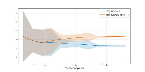
Refer to caption
Figure 12: Evolution of W22subscriptsuperscript𝑊22W^{2}_{2} and min-SWGG w.r.t. the number of points

We observe that, when n𝑛n is large enough, min-SWGG tends to stabilize around some constant value.

We conjecture that there may exist an upper bound for min-SWGG:

min-SWGG22(μ1,μ2)ψ(d,n,d)W22(μ1,μ2)subscriptsuperscriptmin-SWGG22subscript𝜇1subscript𝜇2𝜓𝑑𝑛superscript𝑑subscriptsuperscript𝑊22subscript𝜇1subscript𝜇2\textnormal{min-SWGG}^{2}_{2}(\mu_{1},\mu_{2})\leq\psi(d,n,d^{\prime})W^{2}_{2}(\mu_{1},\mu_{2}) (85)

Where dsuperscript𝑑d^{\prime} is the max of the dimensions of the distributions μ1,μ2subscript𝜇1subscript𝜇2\mu_{1},\mu_{2} [66], and ψ𝜓\psi an unknown function.

E.2 Computing min-SWGG

We now provide here more details about the experimental setup of the experiments of Section 5.1.

Choosing the optimal θ𝜃\theta

We compare three variants for choosing the optimal direction θ𝜃\theta: random search, simulated annealing and optimization (defined in Section 4.3). We choose to compare with simulated annealing since it is widely used in discrete problem (such as the travelling salesman) and known to perform well in high dimension [62] [16] [36]. We notice in Fig. 3 of the paper that the smooth version of min-SWGG is always (comparable or) better than the simulated annealing. In this experiment, we randomly sample 2 Gaussian distributions with different means and covariances matrices, whose parameters are chosen randomly. For optimizing min-SWGG, we use the Adam optimizer of Pytorch, with a fixed learning rate of 5e25superscript𝑒25e^{-2} during 100100100 iterations, considering s=10𝑠10s=10 and ϵ=1italic-ϵ1\epsilon=1.

Fig. 13 provides the timings for computing the random search approximation, simulated annealing and the optimization scheme. In all cases, we recover the linear complexity of min-SWGG (blue curves) in a log space. For the computation timings we compute min-SWGG with random search with L=500𝐿500L=500, simulated annealing (green curves) with 500 iterations with a temperature scheme (1k+1500)k=1500superscriptsubscript1𝑘1500𝑘1500(1-\frac{k+1}{500})_{k=1}^{500} and the optimization scheme (considering s=10𝑠10s=10 with a fixed number of iterations for the optimization scheme equals to 100).
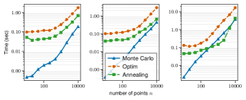
Refer to caption
Figure 13: Considering two Gaussian distributions in dimensions d𝑑d equals to: 2 (left), 20 (middle), 200 (right),we compute min-SWGG with random search, simulated annealing schemes and optimization procedure and report the timings for varying number of points and fixed number of projections.

Additionally, we reproduce the same setup as in 5.1 for the SW, max-SW and PWD distance. For sake of readability we compared with min-SWGG optim and report the results in Fig. 14.
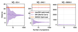
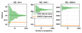
Refer to caption
Refer to caption
Figure 14: Comparison of min-SWGG optim with PWD (left) and with max-SW and SW (right). PWD and SW are computed with a growing number of projection

Runtime Evaluation

In the paper, on Fig. 3 (Right), we compare the empirical runtime evaluation on GPU for different methods. We consider Gaussian distributions in dimension d=3𝑑3d=3 and we sample n𝑛n points per distribution with n{102,103,104,5104,105}𝑛superscript102superscript103superscript1045superscript104superscript105n\in\{10^{2},10^{3},10^{4},5\cdot 10^{4},10^{5}\}. For SW Monte-Carlo and min-SWGG random search, we use L=200𝐿200L=200 projections. For both max-SW and min-SWGG with optimization, we use 100 iterations with a learning rate of 1, and we fix s=50𝑠50s=50 for min-SWGG. We use the official implementation of the Subspace Robust Wasserstein (SRW) with the Frank-Wolfe algorithm [52].

E.3 Gradient Flows

We rely on the code provided with [37] for running the experiment of Section 5.2.

We fix n=100𝑛100n=100, the source distribution is taken to be Gaussian and we consider four different target measures that represent several cases: i) a 2 dimensional Gaussian, ii) a 500 dimensional Gaussian (high dimensional case), iii) 8 Gaussians (multi-modal distribution) and iv) a two-moons distribution (non-linear case).

We fix a global learning rate of 5e35superscript𝑒35e^{-3} with an Adam optimizer. For SW, PWD and SWGG (random search), we sample L=100𝐿100L=100 directions. For the optimization methods max-SW, we set a learning rate of 1e31superscript𝑒31e^{-3} with a number of 100 iterations for i), iii), and iv) and 200 iterations for ii). For min-SWGG (optimization), we took a learning rate of i)1e11superscript𝑒11e^{-1}, ii)1e31superscript𝑒31e^{-3}, iii)5e25superscript𝑒25e^{-2}, and iv) 1e31superscript𝑒31e^{-3}. The hyper parameters for the optimization of min-SWGG are s=10𝑠10s=10 and ϵ=0.5italic-ϵ0.5\epsilon=0.5, except for the 500-dimensional Gaussian for which we pick ϵ=10italic-ϵ10\epsilon=10 .

Each experiment is run 10 times and shaded areas in Fig. 4 (see the main paper) represent the mean ±plus-or-minus\pm the standard deviation.

E.4 Gray scale image colorization

We now provide additional results on a pan-sharpening application to complete results provided in Section 5.3.

In pan-sharpening [64], one aims at constructing a super-resolution multi-chromatic satellite image with the help of a super-resolution mono-chromatic image (source) and low-resolution multi-chromatic image (target).

To realize this task, we choose to used a color transfer procedure, where the idea is to transfer the color palette from the target to the source image. This transfer is carry out by the optimal transport plan of the Wasserstein distance. More details on color transfer can be found in Supp. E.6.

Additionally, we improve the relevance of the colorization by adding a proximity prior. For that, we used super pixels computed via the Watershed algorithm [48] thanks to the the scikit-image package [61]. Obtained high resolution colorized images of size 512×\times512 (n=262 144𝑛262144n=262\leavevmode\nobreak\ 144) are reported on Fig. 15.

Refer to caption
Refer to caption
Refer to caption
Refer to caption
Figure 15: Source high resolution black and white image (left) Target low resolution colorful image (right) Obtained high resolution colorful image (mid).

All pan-sharpening experiments were run on the PairMax data set [64]. The hyperparameters (markers and compactness) for the watershed super-pixels are: 500, 200, 200, 200 markers (an upper bound for the number of super pixel) for each image (by order of apparition) and compactness 1e81𝑒81e-8 (high values result in more regularly-shaped watershed basins) for all the images.

E.5 Point clouds registration

We here provide additional details and results about the experiments in Section 5.4.

Authors of [9] highlighted the relevance of OT in the point clouds registration context, plugged into an Iterative Closest Point (ICP) algorithm. They leveraged the 1D partial OT without consideration for the direction of the line. Our experiment shows the importance of θ𝜃\theta: the smaller SWGG is, the better the registration.

In this experiment, having a one to one correspondence is mandatory: as such, we compare min-SWGG with a nearest neighbor assignment and the one provided by OT. Note that we do not compare min-SWGG with subspace detour [44], since: i) with empirical distributions, the reconstruction of the plan is degenerated (as it doesn’t involve any computation), ii) the research of subspace can be intensive as no prior is provided.

To create the source distributions, we used random transformation (Ω,t)O(d)×dΩ𝑡𝑂𝑑superscript𝑑(\Omega,t)\in O(d)\times\mathbb{R}^{d} of the target domain. ΩΩ\Omega was picked randomly from O(d)𝑂𝑑O(d), the set of rotations and reflections, and t𝑡t has random direction with t2=5subscriptnorm𝑡25\|t\|_{2}=5. We also add a Gaussian noise 𝒩(0,ϵId)𝒩0italic-ϵ𝐼𝑑\mathcal{N}(0,\epsilon Id), with ϵ=0.1italic-ϵ0.1\epsilon=0.1.

The ICP algorithm was run with 3 datasets with the following features: i) 500 points in 2D, ii) 3000 points in 3D, and iii) 150 000 points in 3D. min-SWGG was computed through the random search estimation with L=100𝐿100L=100. A stopping criterion was the maximum number of iterations of the algorithm, which varies with the dataset i.e.: i) 50, ii) 100, and iii) 200 respectively. The other stopping criterion is ΩId+t2εnormΩ𝐼𝑑subscriptnorm𝑡2𝜀\|\Omega-Id\|+\|t\|_{2}\leq\varepsilon with ε𝜀\varepsilon chosen respectively for the datasets as follows: i) 1e41superscript𝑒41e^{-4}, ii) 1e21superscript𝑒21e^{-2}, and iii) 1e21superscript𝑒21e^{-2}, where (Ω,t)O(d)×dΩ𝑡𝑂𝑑superscript𝑑(\Omega,t)\in O(d)\times\mathbb{R}^{d} is the current transformation and \|\cdot\| is the Frobenius norm. All these settings were run with 50 different seeds. Results are reported in Fig. 16.

Refer to caption
Refer to caption
Refer to caption
Figure 16: The three datasets (left) and the distributions of the Sinkhorn divergences, the Chamfer distance, the Frobenius distance, the timing and the number of iterations over 50 seeds (right).

From Fig. 16, one can see that for:

  • n=500𝑛500n=500: The registration obtained via OT is very powerful (it is fast to compute and converges toward a good solution). min-SWGG is slightly faster with better convergence result and an equivalent number of iterations. Finally the nearest neighbor does not converge to a solution closed to the target.

  • n=3000𝑛3000n=3000: registration by OT can converge poorly, moreover the timings are much higher than the competitors. min-SWGG shows efficient convergence results with an attractive computation time (order of fews seconds). We observe that the number of iterations can be very large and we conjecture that it is due to the fact that min-SWGG-based ICP can exit local minima. The nearest neighbor is fast but, most of the time, does not converge to global minima (i.e. the exact matching of the shapes).

  • n=150000𝑛150000n=150000: In this setting, OT is totally untractable (the cost matrix needs 180 GB in memory). min-SWGG shows good convergence and is most of the time very fast whenever the number of iterations does not attain the stopping criterion. The nearest neighbor assignment is faster but only converges to local minima.

Note that, despite the fact that min-SWGG is slightly slower than the nearest neighbor, the overall algorithm can be faster due to the better quality of each iteration (min-SWGG can attain a minimum with less iterations).

In Table 3 we give additional results on the final distribution. We control the final convergence via the square Chamfer distance and the square Frobenius distance. The Square Chamfer distance is a sqaure distance between point cloud defined as:

d2(X,Y)=xXminyYxy22+yYminxXxy22superscript𝑑2𝑋𝑌subscript𝑥𝑋subscriptmin𝑦𝑌subscriptsuperscriptnorm𝑥𝑦22subscript𝑦𝑌subscriptmin𝑥𝑋subscriptsuperscriptnorm𝑥𝑦22\displaystyle d^{2}(X,Y)=\sum_{x\in X}\operatorname*{min}_{y\in Y}||x-y||^{2}_{2}+\sum_{y\in Y}\operatorname*{min}_{x\in X}||x-y||^{2}_{2} (86)

and the Square Frobenius norm is a square distance between the transformation, defined as:

Fr((Ωreal,treal),(Ωestimated,testimated))=ΩrealΩestimated22+trealtestimated22FrsubscriptΩrealsubscript𝑡realsubscriptΩestimatedsubscript𝑡estimatedsubscriptsuperscriptnormsubscriptΩrealsubscriptΩestimated22subscriptsuperscriptnormsubscript𝑡realsubscript𝑡estimated22\displaystyle\text{Fr}((\Omega_{\text{real}},t_{\text{real}}),(\Omega_{\text{estimated}},t_{\text{estimated}}))=\|\Omega_{\text{real}}-\Omega_{\text{estimated}}\|^{2}_{2}+\|t_{\text{real}}-t_{\text{estimated}}\|^{2}_{2} (87)

In both cases we can see that the final results for min-SWGG are much better than the results for NN and relatively closed to the results from OT.

n𝑛n 500 3000 1500 00
NN 11.65 0.20 6.90
OT 0.03 0.16 \cdot
min-SWGG 0.08 0.13 𝟖×𝟏𝟎𝟒8superscript104\boldsymbol{8\times 10^{-4}}
n𝑛n 500 3000 150 000
NN 526 30.04 21.7
OT 3.8 6.5 \cdot
min-SWGG 2 4.5 6.01
Table 3: Square Chamfer distance (top) and Square Frobenius distance (bottom) between final transformation on the source and the target. Best values are boldfaced.

An other important aspect of ICP is that the algorithm tends to fall into local minima: the current solution is not good and further iterations do not allow a better convergence of the algorithm. We observed empirically that min-SWGG can avoid getting stuck on local minima when a reasonable number of directions θ𝜃\theta is sampled (L100similar-to𝐿100L\sim 100). We conjecture that the random search approximation is not always the ideal solution and hence may escape local minima. This may lead to a better convergence solution for min-SWGG-based ICP.

E.6 Color Transfer

In this section, we provide an additional experiment in a color transfer context.

We aim at adapting the color of an input image to match the color of a target one [25, 44]. This problem can be recast as an optimal transport problem where we aim at transporting the color of the source image 𝑿𝑿\boldsymbol{X} into the target 𝒀𝒀\boldsymbol{Y}. For that, usual methods lie down on the existence of a map T:𝑿𝒀:𝑇𝑿𝒀T:\boldsymbol{X}\to\boldsymbol{Y}. We challenge min-SWGG to this problem to highlight relevance of the obtained transport map.

Images are encoded as vector in nm×3superscript𝑛𝑚3\mathbb{R}^{nm\times 3}, where n𝑛n and m𝑚m are the size of the image and 333 corresponds to the number of channels (here RBG channels). We first compute a map T0:𝑿0𝒀0:subscript𝑇0subscript𝑿0subscript𝒀0T_{0}:\boldsymbol{X}_{0}\to\boldsymbol{Y}_{0} between a subsample of 𝑿𝑿\boldsymbol{X} and 𝒀𝒀\boldsymbol{Y} of size 20000 and secondly extend this mapping to the complete distributions T:𝑿𝒀:𝑇𝑿𝒀T:\boldsymbol{X}\to\boldsymbol{Y} using a nearest neighbor interpolation. The subsampling step is mandatory due to the size of the images but can deteriorate the quality of the transfer.

We compare the results obtained with maps obtained from Wasserstein distance, min-SWGG with random search (100 projections), subspace detour [44] and min-SWGG (optimized). Obtained images and the associated timings are provided in fig. 17.

Refer to caption
Refer to caption
Figure 17: Color transfer of images with W22subscriptsuperscript𝑊22W^{2}_{2}, min-SWGG and subspace detours, with runtimes.

Figure 17 shows that min-SWGG and W22superscriptsubscript𝑊22W_{2}^{2} provide visually equivalent solutions. Since, the quality of the color transfer is dependent on the size of the subsampling: using min-SWGG permits larger subsamples than W22subscriptsuperscript𝑊22W^{2}_{2} and thus improves the quality of the map T𝑇T. Moreover one can note that min-SWGG (optimized) is the fastest to compute.

We now give more details about how to perform color transfer between two distributions. The first step is to encode n×m𝑛𝑚n\times m images as nm×3superscript𝑛𝑚3\mathbb{R}^{nm\times 3} vectors, with 3 channels in a RGB image. Note that m𝑚m and n𝑛n can differ for the source and target image. The second step consists of defining subsamples X0,Y0subscript𝑋0subscript𝑌0X_{0},Y_{0} of X,Y𝑋𝑌X,Y, in our case we took 𝑿0,𝒀020000×dsubscript𝑿0subscript𝒀0superscript20000𝑑\boldsymbol{X}_{0},\boldsymbol{Y}_{0}\in\mathbb{R}^{20000\times d}. We subsample the same number of points for the source and target image. In order to have a better subsampling of 𝑿𝑿\boldsymbol{X} and 𝒀𝒀\boldsymbol{Y}, it is common to perform a k𝑘k-means [34] to derive 𝑿0subscript𝑿0\boldsymbol{X}_{0} and 𝒀0subscript𝒀0\boldsymbol{Y}_{0} (𝑿0,𝒀0subscript𝑿0subscript𝒀0\boldsymbol{X}_{0},\boldsymbol{Y}_{0} are then taken as centroids of the k-means algorithm). The third step is to compute T0:𝑿0𝒀0:subscript𝑇0subscript𝑿0subscript𝒀0T_{0}:\boldsymbol{X}_{0}\to\boldsymbol{Y}_{0}. We set T𝑇T as the optimal Monge map given by the Wasserstein distance and T𝑇T as the optimal map given by min-SWGG. Finally, the fourth step deals with extending T0:𝑿0𝒀0:subscript𝑇0subscript𝑿0subscript𝒀0T_{0}:\boldsymbol{X}_{0}\to\boldsymbol{Y}_{0} to T:𝑿𝒀:𝑇𝑿𝒀T:\boldsymbol{X}\to\boldsymbol{Y}. 𝒙𝑿for-all𝒙𝑿\forall\boldsymbol{x}\in\boldsymbol{X}. We compute the closest element 𝒙0𝑿0subscript𝒙0subscript𝑿0\boldsymbol{x}_{0}\in\boldsymbol{X}_{0} and we pose:

T(𝒙)=T(𝒙0).𝑇𝒙𝑇subscript𝒙0T(\boldsymbol{x})=T(\boldsymbol{x}_{0}). (88)

More details on the overall procedure can be found in [25].

To perform the experiment, we took L=100𝐿100L=100 projections for min-SWGG (random search). For min-SWGG (optimized), we fixed the following set of parameters for the gradient descent: learning rate 5e25superscript𝑒25e^{-2}, number of iterations 20, number of copies s=10𝑠10s=10 and ϵ=1italic-ϵ1\epsilon=1. Regarding the subspace detour results, we used the code of [44] provided at https://github.com/BorisMuzellec/SubspaceOT.

Additionally, we perform color transfer without sub-sampling with the help of min-SWGG (we the same hyperparameters). This procedure is totally untractable for either W22subscriptsuperscript𝑊22W^{2}_{2} and subspace detours (due to memory issues). As we mentioned before, the subsampling phase can decrease the quality of the transfer and thus min-SWGG can deliver better result than before. Result are give in Fig. 18

Refer to caption
Figure 18: Color transfer of images with min-SWGG without sub-sampling.

E.7 Data set distance

We finally evaluate min-SWGG in an other context: computing distances between datasets. Let 𝒟1={(𝒙i1,𝒚i1)}i=1nsubscript𝒟1superscriptsubscriptsubscriptsuperscript𝒙1𝑖subscriptsuperscript𝒚1𝑖𝑖1𝑛\mathcal{D}_{1}=\{(\boldsymbol{x}^{1}_{i},\boldsymbol{y}^{1}_{i})\}_{i=1}^{n} and 𝒟2={(𝒙i2,𝒚i2)}i=1nsubscript𝒟2superscriptsubscriptsubscriptsuperscript𝒙2𝑖subscriptsuperscript𝒚2𝑖𝑖1𝑛\mathcal{D}_{2}=\{(\boldsymbol{x}^{2}_{i},\boldsymbol{y}^{2}_{i})\}_{i=1}^{n} be source and target data sets such that 𝒙i1,𝒙i2dsubscriptsuperscript𝒙1𝑖subscriptsuperscript𝒙2𝑖superscript𝑑\boldsymbol{x}^{1}_{i},\boldsymbol{x}^{2}_{i}\in\mathbb{R}^{d} are samples and 𝒚i1,𝒚i2superscriptsubscript𝒚𝑖1superscriptsubscript𝒚𝑖2\boldsymbol{y}_{i}^{1},\boldsymbol{y}_{i}^{2} are labels 1infor-all1𝑖𝑛\forall 1\leq i\leq n. In [3], the authors compare those data sets using the Wasserstein distance with the entries of the cost matrix defined as:

Cij=(𝒙i1𝒙j222+W22(α𝒚i1,α𝒚j2))1/2subscript𝐶𝑖𝑗superscriptsubscriptsuperscriptnormsubscriptsuperscript𝒙1𝑖subscriptsuperscript𝒙2𝑗22subscriptsuperscript𝑊22subscript𝛼superscriptsubscript𝒚𝑖1subscript𝛼superscriptsubscript𝒚𝑗212\displaystyle C_{ij}=\left(\|\boldsymbol{x}^{1}_{i}-\boldsymbol{x}^{2}_{j}\|^{2}_{2}+W^{2}_{2}(\alpha_{\boldsymbol{y}_{i}^{1}},\alpha_{\boldsymbol{y}_{j}^{2}})\right)^{1/2} (89)

and the corresponding distance as:

OTDD(𝒟1,𝒟2)=minPUC,P𝑂𝑇𝐷𝐷subscript𝒟1subscript𝒟2subscript𝑃𝑈𝐶𝑃\displaystyle OTDD(\mathcal{D}_{1},\mathcal{D}_{2})=\min_{P\in U}\langle C,P\rangle (90)

where α𝒚subscript𝛼𝒚\alpha_{\boldsymbol{y}} is the distribution of all samples with label 𝒚𝒚\boldsymbol{y}, namely {𝒙d|(𝒙,𝒚)𝒟}conditional-set𝒙superscript𝑑𝒙𝒚𝒟\{\boldsymbol{x}\in\mathbb{R}^{d}|(\boldsymbol{x},\boldsymbol{y})\in\mathcal{D}\} for 𝒟𝒟\mathcal{D} being either 𝒟1subscript𝒟1\mathcal{D}_{1} or 𝒟2subscript𝒟2\mathcal{D}_{2} and U𝑈U is the Birkhoff polytope which encodes the marginal constraints. Notice that cost in Eq. (89) encompasses the ground distance and a label-to-label distance. This distance is appealing in transfer learning application since it is model-agnostic. However, it can be cumbersome to compute in practice since it lays down on solving multiple OT problems (to compute the cost matrix and the OTDD). To circumvent that, [3] proposed several methods to compute the cost matrix in Eq. (89). They used the Sinkhorn algorithm (in 𝒪(n2)𝒪superscript𝑛2\mathcal{O}(n^{2})) or they assumed α𝒚𝒩(m𝒚,Σ𝒚)similar-tosubscript𝛼𝒚𝒩subscript𝑚𝒚subscriptΣ𝒚\alpha_{\boldsymbol{y}}\sim\mathcal{N}(m_{\boldsymbol{y}},\Sigma_{\boldsymbol{y}}) in order to get the WD through the Bures metric (that provides a closed form of OT for Gaussian distributions in 𝒪(d3)𝒪superscript𝑑3\mathcal{O}(d^{3})), which is still prohibitive for high dimension. We challenge min-SWGG in this context.

In this experiment, we compare the following datasets: MNIST [39], EMNIST [18], FashionMNIST [67], KMNIST [17] and USPS [32]. We rely on the code of OTDD provided at https://github.com/microsoft/otdd. In order to make it compliant with the min-SWGG hypothesis, we require the empirical distributions α𝒚subscript𝛼𝒚\alpha_{\boldsymbol{y}} to have the same number of atoms.

Fig. 19 provides results for a batch size of n=40000𝑛40000n=40000 samples using the Sinkhorn divergence (with a regularisation parameter of 1e11superscript𝑒11e^{-1}) and for min-SWGG (optimized) on batch of size 40000. We report results for a learning rate of 1e51superscript𝑒51e^{-5}, 20 iterations and s𝑠s and ϵitalic-ϵ\epsilon to be 1 and 0.

110.81.11.21.21.311.31.21.30.811.21.2111.31.21MNISTEMNISTFashionKMNISTUSPSMNISTEMNISTFashionKMNISTUSPS
0.90.90.70.91.111.20.91.21.31.20.80.81.11.10.90.91.21.10.9MNISTEMNISTFashionKMNISTUSPSMNISTEMNISTFashionKMNISTUSPS
Figure 19: OTDD results (×102absentsuperscript102\times 10^{2}) distances for min-SWGG (left) and Sinkhorn divergence (right) for various datasets.

We check that the orders of magnitude are preserved with min-SWGG. For example OTDD(MNIST,USPS) is smaller than OTDD(MNIST,FashionMNIST) for either Sinkhorn divergence or min-SWGG as distance between labels, this validate that min-SWGG is a meaningful distance in this case scenario. Moreover in our setup, the computation cost is more expensive for Sinkhorn than for min-SWGG and totally untractable for W22subscriptsuperscript𝑊22W^{2}_{2}. On smaller batches (see Fig 20), the same observation can be made: min-SWGG is comparable (in term of magnitude) with W22subscriptsuperscript𝑊22W^{2}_{2}, Sinkhorn and the Bures approximation.

We give additional results in Fig. 20 for batches of size of n=2000𝑛2000n=2000 samples obtained with W22subscriptsuperscript𝑊22W^{2}_{2}, Sinkhorn divergence (setting the entropic regularization parameter to 1e11superscript𝑒11e^{-1}), the Bures approximation, min-SWGG (random search with L=1000𝐿1000L=1000 projections) and min-SWGG (optimized, with a learning rate of 5e15superscript𝑒15e^{-1}, 50 iterations, s=20𝑠20s=20 and ϵ=0.5italic-ϵ0.5\epsilon=0.5).

0.40.50.40.40.50.50.60.40.60.50.60.30.40.50.50.40.40.60.50.4MNISTEMNISTFashionKMNISTUSPSMNISTEMNISTFashionKMNISTUSPS
110.811.21.21.311.31.21.30.80.91.21.210.91.31.20.9MNISTEMNISTFashionKMNISTUSPSMNISTEMNISTFashionKMNISTUSPS
0.90.90.70.9111.10.91.21.11.10.70.81.110.90.81.110.8MNISTEMNISTFashionKMNISTUSPSMNISTEMNISTFashionKMNISTUSPS
11.10.91.11.31.31.41.11.31.31.40.811.31.31.111.31.31.1MNISTEMNISTFashionKMNISTUSPSMNISTEMNISTFashionKMNISTUSPS
11.10.81.11.31.31.31.11.31.21.40.811.31.31.111.31.31MNISTEMNISTFashionKMNISTUSPSMNISTEMNISTFashionKMNISTUSPS
Figure 20: OTDD distance with W22subscriptsuperscript𝑊22W^{2}_{2} (left), Sinkhorn (left-mid), Bures (middle) and random search min-SWGG (right-mid) and min-SWGG-optimization (right) distances between labels distribution ×102absentsuperscript102\times 10^{2}

Note that the Figs. 19 and 20 are not symmetric (OTDD(KMNIST,FashionMNIST)\neq OTDD(FashinMNIST,KMNIST)) because of the random aspect of batches.