Nonparametric Classification on Low Dimensional Manifolds using Overparameterized Convolutional Residual Networks

Abstract

Convolutional residual neural networks (ConvResNets), though overparameterized, can achieve remarkable prediction performance in practice, which cannot be well explained by conventional wisdom. To bridge this gap, we study the performance of ConvResNeXts, which cover ConvResNets as a special case, trained with weight decay from the perspective of nonparametric classification. Our analysis allows for infinitely many building blocks in ConvResNeXts, and shows that weight decay implicitly enforces sparsity on these blocks. Specifically, we consider a smooth target function supported on a low-dimensional manifold, then prove that ConvResNeXts can adapt to the function smoothness and low-dimensional structures and efficiently learn the function without suffering from the curse of dimensionality. Our findings partially justify the advantage of overparameterized ConvResNeXts over conventional machine learning models.

1 Introduction

Deep learning has achieved significant success in various real-world applications, such as computer vision [9, 15, 19], natural language processing [1, 10, 31], and robotics [11]. One notable example of this is in the field of image classification, where the winner of the 2017 ImageNet challenge achieved a top-5 error rate of just 2.25% [13] using ConvResNets on a training dataset of 1 million labeled high-resolution images in 1000 categories.

Among various deep learning models, ConvResNets have gained widespread popularity in practical applications [3, 12, 24, 33]. Compared to vanilla feedforward neural networks (FNNs), ConvResNets possess two distinct features: convolutional layers and skip connections. Specifically, each block of ConvResNets consists of a subnetwork, called bottleneck, and an identity connection between inconsecutive blocks. The identity connection effectively mitigates the vanishing gradient issue. Each layer of the bottleneck contains several filters (channels) that convolve with the input. Using this ConvResNet architecture, He et al. [12] won 1st place on the ImageNet classification task with a 3.57% top-5 error in 2015. ConvResNets have various extensions, one of which is ConvResNeXts [29]. This structure generalizes ConvResNets and includes them as a special case. Each building block in ConvResNeXts has a parallel architecture that enables multiple “paths” within the block. This approach allows for improving the performance without increasing the number of parameters.

There are few theoretical works about ConvResNet, despite its remarkable empirical success. Previous research has focused on the representation power of FNNs [2, 4, 14, 23, 30], while limited literature exists on ConvResNets. Oono and Suzuki [21] developed a representation and statistical estimation theory of ConvResNets, and showed that if the network architecture is appropriately designed, ConvResNets with $O(n^{D/(2\alpha+D)})$ blocks can achieve a minimax optimal convergence rate $\tilde{O}(n^{-2\alpha/(2\alpha+D)})$ when approximating a $C^{\alpha}$ function with $n$ samples. Additionally, Liu et al. [18] proved that ConvResNets can universally approximate any function in the Besov space $B^{\alpha}_{p,q}$ on $d$-dimensional manifolds with arbitrary accuracy. They improved the convergence rate to $\tilde{O}(n^{-2\alpha/(2\alpha+d)})$ for ConvResNets with $O(n^{d/(2\alpha+d)})$ blocks. Their results only depend on the intrinsic dimension $d$, rather than the data dimension $D$.

These previous works, however, have limitations in explaining the success of ConvResNets achieved by overparameterization, where the number of blocks can be much larger than the sample size. In practice, the performance of ConvResNets becomes better when they go deeper [12, 28], but the previous results required a finite number of blocks and thus cannot explain this phenomenon. For instance, Liu et al. [18] shows that the number of blocks for ConvResNets is $O(n^{d/(2\alpha+d)})$. Since the intrinsic dimension is typically small, the number of blocks cannot be too large, as tremendous blocks in ConvResNets result in a bad convergence rate.

To bridge this gap, we study ConvResNeXts under an overparameterization regime [29]. The ConvResNeXt is an extension to the ConvResNet and can cover ConvResNets as a special case. Our paper considers a nonparametric classification problem using ConvResNeXts trained by weight decay. We show that overparameterized ConvResNeXts can achieve an asymptotic minimax rate for estimating Besov functions. Specifically, assuming the target function is supported on a $d$-dimensional manifold and belongs to the Besov space $B^{\alpha}_{p,q}$, we prove that the estimator given by the ConvResNeXt class can converge to the target function at the rate $\tilde{O}(n^{-\frac{\alpha/d}{2\alpha/d+1}(1-o(1))})$ with $n$ samples. Here, weight decay is a common method in deep learning to reduce overfitting [16, 22]. With this approach, ConvResNeXts can have infinitely many blocks to achieve arbitrary accuracy, which corresponds to the real-world applications [12, 28].

Our work is partially motivated by Zhang and Wang [32]. However, our work distinguishes itself through two remarkable technical advancements. Firstly, we develop approximation theory for ConvResNeXts, while Zhang and Wang [32] only focuses on FNNs. In addition, we take into account low-dimensional geometric structures of data. Specifically, we consider approximating any function in Besov space $B^{\alpha}_{p,q}$ on a $d$-dimensional manifold and show that the network consisting of at most $O(\epsilon^{-d/\alpha})$ blocks and $O(\log(1/\epsilon))$ layers in each block can achieve an $\epsilon$-approximation error. Notably, the network size in our theory only depends on the intrinsic dimension $d$, which circumvents the curse of dimensionality. Another technical highlight of our paper is bounding the covering number of weight-decayed ConvResNeXts, which is essential for computing the critical radius of the local Gaussian complexity. This technique provides a tighter bound than choosing a single radius of the covering number as in Suzuki [23], Zhang and Wang [32]. To the best of our knowledge, our work is the first to develop approximation theory and statistical estimation results for ConvResNeXts.

The rest of this paper is organized as follows: Section 2 introduces preliminaries on smooth manifolds, function approximation, and ConvResNeXt architectures; Section 3 presents our main results; Section 4 presents a proof sketch of our theory; Section 5 draws a brief conclusion.

2 Preliminaries

In this section, we introduce some concepts on manifolds. Details can be found in [26] and [17]. Then we provide a detailed definition of Besov spaces on smooth manifolds and the ConvResNeXt architecture.

2.1 Smooth manifold

Firstly, we briefly introduce manifolds, the partition of unity and reach. Let $\mathcal{M}$ be a $d$-dimensional Riemannian manifold isometrically embedded in $\mathbb{R}^{D}$ with $d$ much smaller than $D$.

Definition 1 (Chart).

A chart on $\mathcal{M}$ is a pair $(U,\phi)$ such that $U\subset\mathcal{M}$ is open and $\phi:U\mapsto\mathbb{R}^{d},$ where $\phi$ is a homeomorphism (i.e., bijective, $\phi$ and $\phi^{-1}$ are both continuous).

In a chart $(U,\phi)$, $U$ is called a coordinate neighborhood, and $\phi$ is a coordinate system on $U$. Essentially, a chart is a local coordinate system on $\mathcal{M}$. A collection of charts that covers $\mathcal{M}$ is called an atlas of $\mathcal{M}$.

Definition 2 ($C^{k}$ Atlas).

A $C^{k}$ atlas for $\mathcal{M}$ is a collection of charts $\{(U_{i},\phi_{i})\}_{i\in\mathcal{A}}$ which satisfies $\bigcup_{i\in\mathcal{A}}U_{i}=\mathcal{M}$, and are pairwise $C^{k}$ compatible:

$$\phi_{i}\circ\phi_{\beta}^{-1}:\phi_{\beta}(U_{i}\cap U_{\beta})\to\phi_{i}(U_{i}\cap U_{\beta})\quad\textrm{and}\quad\phi_{\beta}\circ\phi_{i}^{-1}:\phi_{i}(U_{i}\cap U_{\beta})\to\phi_{\beta}(U_{i}\cap U_{\beta})$$

are both $C^{k}$ for any $i,\beta\in\mathcal{A}$. An atlas is called finite if it contains finitely many charts.

Definition 3 (Smooth Manifold).

A smooth manifold is a manifold $\mathcal{M}$ together with a $C^{\infty}$ atlas.

Classical examples of smooth manifolds are the Euclidean space, the torus, and the unit sphere. Furthermore, we define $C^{s}$ functions on a smooth manifold $\mathcal{M}$ as follows:

Definition 4 ($C^{s}$ functions on $\mathcal{M}$).

Let $\mathcal{M}$ be a smooth manifold and $f:\mathcal{M}\rightarrow\mathbb{R}$ be a function on $\mathcal{M}$. A function $f:\mathcal{M}\to\mathbb{R}$ is $C^{s}$ if for any chart $(U,\phi)$ on $\mathcal{M}$, the composition $f\circ\phi^{-1}:\phi(U)\rightarrow\mathbb{R}$ is a continuously differentiable up to order $s$.

We next define the $C^{\infty}$ partition of unity, which is an important tool for studying functions on manifolds.

Definition 5 (Partition of Unity, Definition 13.4 in [26]).

A $C^{\infty}$ partition of unity on a manifold $\mathcal{M}$ is a collection of $C^{\infty}$ functions $\{\rho_{i}\}_{i\in\mathcal{A}}$ with $\rho_{i}:\mathcal{M}\to[0,1]$ such that for any $\boldsymbol{x}\in\mathcal{M}$,

1. there is a neighbourhood of $\boldsymbol{x}$ where only a finite number of the functions in $\{\rho_{i}\}_{i\in\mathcal{A}}$ are nonzero;

2. $\displaystyle\sum_{i\in\mathcal{A}}\rho_{i}(\boldsymbol{x})=1$.

An open cover of a manifold $\mathcal{M}$ is called locally finite if every $\boldsymbol{x}\in\mathcal{M}$ has a neighborhood that intersects with a finite number of sets in the cover. The following proposition shows that a $C^{\infty}$ partition of unity for a smooth manifold always exists.

Proposition 1 (Existence of a $C^{\infty}$ partition of unity, Theorem 13.7 in [26]).

Let $\{U_{i}\}_{i\in\mathcal{A}}$ be a locally finite cover of a smooth manifold $\mathcal{M}$. Then there is a $C^{\infty}$ partition of unity $\{\rho_{i}\}_{i=1}^{\infty}$ where every $\rho_{i}$ has a compact support such that $\mathrm{supp}(\rho_{i})\subset U_{i}$.

Let $\{(U_{i},\phi_{i})\}_{i\in\mathcal{A}}$ be a $C^{\infty}$ atlas of $\mathcal{M}$. Proposition 1 guarantees the existence of a partition of unity $\{\rho_{i}\}_{i\in\mathcal{A}}$ such that $\rho_{i}$ is supported on $U_{i}$. To characterize the curvature of a manifold, we adopt the geometric concept: reach.

Definition 6 (Reach [7, 20]).

Denote

$$G=\left\{\boldsymbol{x}\in\mathbb{R}^{D}:\exists~{}\boldsymbol{p}\neq\boldsymbol{q}\in\mathcal{M}\mbox{ such that }\|\boldsymbol{x}-\boldsymbol{p}\|_{2}=\|\boldsymbol{x}-\boldsymbol{q}\|_{2}\}=\inf_{\boldsymbol{y}\in\mathcal{M}}\|\boldsymbol{x}-\boldsymbol{y}\|_{2}\right\}.$$

as the set of points with at least two nearest neighbors on $\mathcal{M}$. The closure of $G$ is called the medial axis of $\mathcal{M}$. Then the reach of $\mathcal{M}$ is defined as

$$\tau=\inf_{\boldsymbol{x}\in\mathcal{M}}\ \inf_{\boldsymbol{y}\in G}\|\boldsymbol{x}-\boldsymbol{y}\|_{2}.$$

Reach has a simple geometrical interpretation: for every point $\boldsymbol{x}\in\mathcal{M}$, the osculating circle’s radius is at least $\tau$. A large reach for $\mathcal{M}$ indicates that the manifold changes slowly.

2.2 Besov functions on a smooth manifold

We next define Besov function spaces on the smooth manifold $\mathcal{M}$, which generalizes more elementary function spaces such as the Sobolev and Hölder spaces. To define Besov functions, we first introduce the modulus of smoothness.

Definition 7 (Modulus of Smoothness [5, 23]).

Let $\Omega\subset\mathbb{R}^{D}$. For a function $f:\mathbb{R}^{D}\rightarrow\mathbb{R}$ be in $L^{p}(\Omega)$ for $p>0$, the $r$-th modulus of smoothness of $f$ is defined by

$$w_{r,p}(f,t)=\sup_{\|\boldsymbol{h}\|_{2}\leq t}\|\Delta_{\boldsymbol{h}}^{r}(f)\|_{L^{p}},\mbox{ where}$$

$$\Delta_{\boldsymbol{h}}^{r}(f)(\boldsymbol{x})=\begin{cases}\sum_{j=0}^{r}\binom{r}{j}(-1)^{r-j}f(\boldsymbol{x}+j\boldsymbol{h})&\mbox{ if }\ \boldsymbol{x}\in\Omega,\boldsymbol{x}+r\boldsymbol{h}\in\Omega,\\ 0&\mbox{ otherwise}.\end{cases}$$

Definition 8 (Besov Space $B_{p,q}^{\alpha}(\Omega)$).

For $0<p,q\leq\infty,\alpha>0,r=\lfloor\alpha\rfloor+1$, define the seminorm $|\cdot|_{B_{p,q}^{\alpha}}$ as

$$|f|_{B_{p,q}^{\alpha}(\Omega)}:=\begin{cases}\left(\displaystyle\int_{0}^{\infty}(t^{-\alpha}w_{r,p}(f,t))^{q}\frac{dt}{t}\right)^{\frac{1}{q}}&\mbox{ if }q<\infty,\\ \sup_{t>0}t^{-\alpha}w_{r,p}(f,t)&\mbox{ if }q=\infty.\end{cases}$$

The norm of the Besov space $B_{p,q}^{s}(\Omega)$ is defined as $\|f\|_{B_{p,q}^{\alpha}(\Omega)}:=\|f\|_{L^{p}(\Omega)}+|f|_{B_{p,q}^{\alpha}(\Omega)}$. Then the Besov space is defined as $B_{p,q}^{\alpha}(\Omega)=\{f\in L^{p}(\Omega)|\|f\|_{B_{p,q}^{\alpha}}<\infty\}$.

Moreover, we show that functions in Besov space can be decomposed using B-spline basis functions in the following proposition.

Proposition 2 (Decomposition of Besov functions).

Any function $f$ in Besov space $B^{\alpha}_{p,q},\alpha>d/p$ can be decomposed using B-spline of order $m,m>\alpha$: for any $\boldsymbol{x}\in\mathbb{R}^{d}$, we have

$$f(\boldsymbol{x})=\sum_{k=0}^{\infty}\sum_{\boldsymbol{s}\in J(k)}c_{k,\boldsymbol{s}}(f)M_{m,k,\boldsymbol{s}}(\boldsymbol{x}),$$ (1)

where $J(k):=\{2^{-k}\boldsymbol{s}:\boldsymbol{s}\in[-m,2^{k}+m]^{d}\subset\mathbb{Z}^{d}\}$, $M_{m,k,\boldsymbol{s}}(\boldsymbol{x}):=M_{m}(2^{k}(\boldsymbol{x}-\boldsymbol{s}))$, and $M_{k}(\boldsymbol{x})=\prod_{i=1}^{d}M_{k}(x_{i})$ is the cardinal B-spline basis function which can be expressed as a polynomial:

$$M_{m}(z) =\frac{1}{m!}\sum_{j=1}^{m+1}(-1)^{j}{m+1\choose j}(z-j)^{m}_{+}$$ (2)

$$=((m+1)/2)^{m}\frac{1}{m!}\sum_{j=1}^{m+1}(-1)^{j}{m+1\choose j}\left(\frac{z-j}{(m+1)/2}\right)^{m}_{+}.$$

We next define $B_{p,q}^{\alpha}$ functions on $\mathcal{M}$.

Definition 9 ($B_{p,q}^{\alpha}$ Functions on $\mathcal{M}$ [8, 25]).

Let $\mathcal{M}$ be a compact smooth manifold of dimension $d$. Let $\{(U_{i},\phi_{i})\}_{i=1}^{C_{\mathcal{M}}}$ be a finite atlas on $\mathcal{M}$ and $\{\rho_{i}\}_{i=1}^{C_{\mathcal{M}}}$ be a partition of unity on $\mathcal{M}$ such that $\mathrm{supp}(\rho_{i})\subset U_{i}$. A function $f:\mathcal{M}\to\mathbb{R}$ is in $B_{p,q}^{\alpha}(\mathcal{M})$ if

$$\|f\|_{B_{p,q}^{\alpha}(\mathcal{M})}:=\sum_{i=1}^{C_{\mathcal{M}}}\|(f\rho_{i})\circ\phi_{i}^{-1}\|_{B_{p,q}^{\alpha}(\mathbb{R}^{d})}<\infty.$$ (3)

Since $\rho_{i}$ is supported on $U_{i}$, the function $(f\rho_{i})\circ\phi_{i}^{-1}$ is supported on $\phi(U_{i})$. We can extend $(f\rho_{i})\circ\phi_{i}^{-1}$ from $\phi(U_{i})$ to $\mathbb{R}^{d}$ by setting the function to be $0$ on $\mathbb{R}^{d}\setminus\phi(U_{i})$. The extended function lies in the Besov space $B^{s}_{p,q}(\mathbb{R}^{d})$ [25, Chapter 7].

2.3 Architecture of ConvResNeXt

In this part, we provide the architecture of ConvResNeXts. This structure has three main features: convolution kernel, residual connections, and parallel architecture.

Consider one-sided stride-one convolution in our network. Let $\mathcal{W}=\{\mathcal{W}_{j,k,l}\}\in\mathbb{R}^{w^{\prime}\times K\times w}$ be a convolution kernel with output channel size $w^{\prime}$, kernel size $K$ and input channel size $w$. For $\boldsymbol{z}\in\mathbb{R}^{D\times w}$, the convolution of $\mathcal{W}$ with $\boldsymbol{z}$ gives $\boldsymbol{y}\in\mathbb{R}^{D\times w^{\prime}}$ such that

$$\boldsymbol{y}=\mathcal{W}\star\boldsymbol{z},\quad y_{i,j}=\sum_{k=1}^{K}\sum_{l=1}^{w}\mathcal{W}_{j,k,l}z_{i+k-1,l},$$ (4)

where $1\leq i\leq D,1\leq j\leq w^{\prime}$ and we set $z_{i+k-1,l}=0$ for $i+k-1>D$, as demonstrated in Figure 1(a).

The building blocks of ConvResNeXts are residual blocks. Given an input $\boldsymbol{x}$, each residual block computes $\boldsymbol{x}+F(\boldsymbol{x})$, where $F$ is a subnetwork called bottleneck, consisting of convolutional layers.

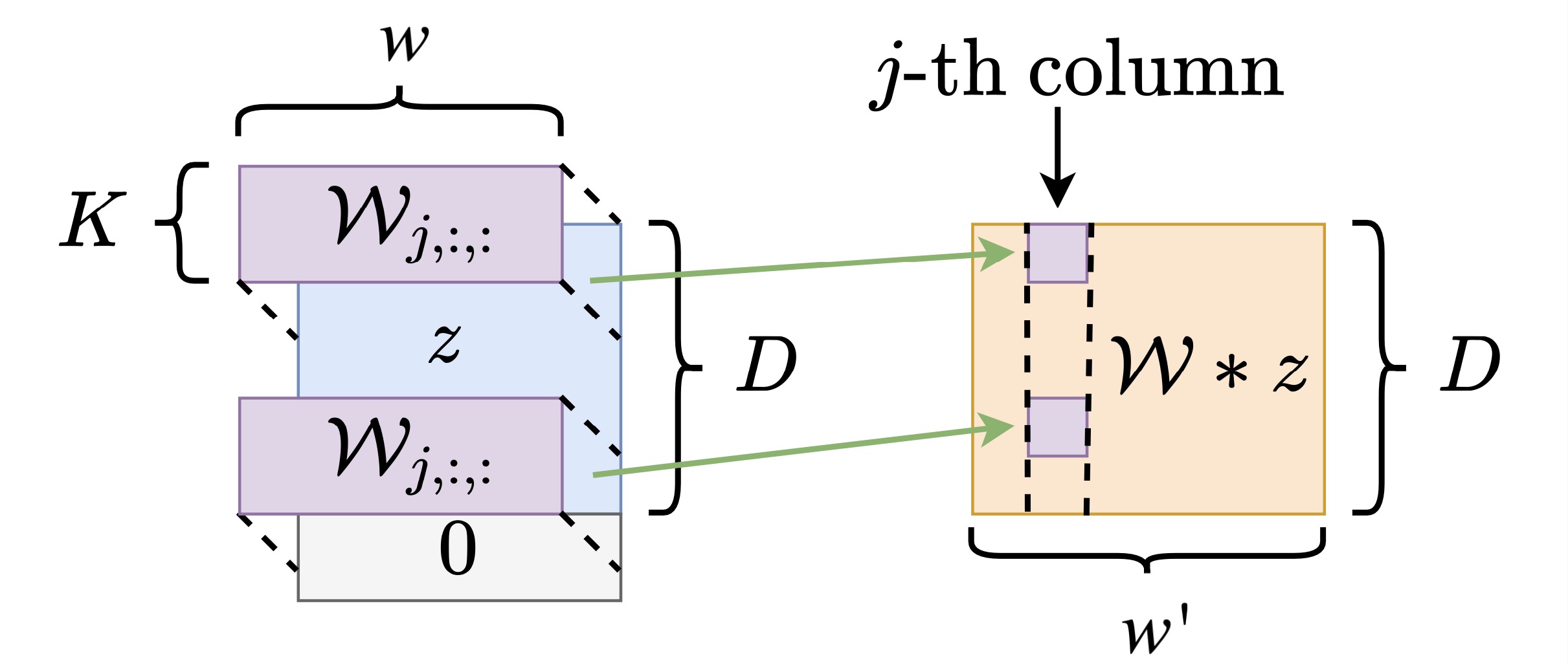
((a))

((b))

Figure 1: (a) Demonstration of the convolution operation $\mathcal{W}*z$, where the input is $z\in\mathbb{R}^{D\times w}$, and the output is $\mathcal{W}*z\in\mathbb{R}^{D\times w^{\prime}}$. Here $\mathcal{W}_{j,:,:}$ is a $D\times w$ matrix for the $j$-th output channel. (b) Demonstration of the ConvResNeXt. $f_{1,1}\dots f_{N,M}$ are the building blocks, each building block is a convolution neural network.

In ConvResNeXts, a parallel architecture is introduced to each building block, which enables multiple “paths” in each block. This approach allows for improving the performance without increasing the number of parameters. In this paper, we study the ConvResNeXts with rectified linear unit (ReLU) activation function, i.e., $\mathrm{ReLU}(z)=\max\{z,0\}$. We next provide the detailed definition of ConvResNeXts as follows:

Definition 10.

Let the neural network comprise $N$ residual blocks, each building block has a parallel architecture with $M$ building blocks, and each building block contains $L$ layers. The number of channels is $w$, and the convolution kernel size is $K$. Given an input $\boldsymbol{x}\in\mathbb{R}^{D}$, a ConvResNeXt with ReLU activation function can be represented as

$$f(\boldsymbol{x}) =\mathbf{W}_{out}\cdot\left(\sum_{m=1}^{M}f_{N,m}+\mathrm{id}\right)\circ\dots\circ\left(\sum_{m=1}^{M}f_{1,m}+\mathrm{id}\right)\circ P(\boldsymbol{x}),$$

$$f_{n,m} =\mathbf{W}_{L}^{(n,m)}\star\mathrm{ReLU}\left(\mathbf{W}_{L-1}^{(n,m)}\star\dots\star\mathrm{ReLU}\left(\mathbf{W}_{1}^{(n,m)}\star\boldsymbol{x}\right)\right),$$

where $\mathrm{id}$ is the identity operator, $P:\mathbb{R}^{D}\to\mathbb{R}^{D\times w_{0}}$ is the padding operator satisfying $P(\boldsymbol{x})=[\boldsymbol{x},~{}~{}\boldsymbol{0}~{}~{}\dots~{}~{}\boldsymbol{0}]\in\mathbb{R}^{D\times w}$, $\{\mathbf{W}_{l}^{(n,m)}\}_{l=1}^{L}$ is a collection of convolution kernels for $n=1,\ldots,N,m=1,\ldots,M$, $\mathbf{W}_{\rm{out}}\in\mathbb{R}^{w_{L}}$ denotes the linear operator for the last layer, and $\star$ is the convolution operation defined in (missing) 4.

The structure of ConvResNeXts is shown in Figure 1(b). When $M=1$, the ConvResNeXt defined in 10 reduces to a ConvResNet. Without loss of generality, we assume that all the building blocks in the neural network contain no bias. The missing representation power from the bias can be compensated by padding the input with a scalar ‘1’. The channel with “0” is used to accumulate the output. See 18 for details.

3 Theory

In this section, we study a binary classification problem on $\mathcal{M}$. Specifically, we are given i.i.d. sample $\{\boldsymbol{x}_{i},y_{i}\}_{i=1}^{n}\sim\mathcal{D}$ where $\boldsymbol{x}_{i}\in\mathcal{M}$ and $y_{i}\in\{0,1\}$ is the label. The label $y$ follows the Bernoulli-type distribution

$$\mathbb{P}(y=1|\boldsymbol{x})=\eta(\boldsymbol{x}),~{}~{}\mathbb{P}(y=0|\boldsymbol{x})=1-\eta(\boldsymbol{x})$$

for some $\eta:\mathcal{M}\to[0,1]$. In binary classification, a classifier $f$ predicts the label of $\boldsymbol{x}$ as $\mathrm{sign}(f(\boldsymbol{x})-c)$ for some threshold constant $c\in\mathbb{R}$. To learn the optimal classifier, we consider a loss function $\mathrm{Loss}(\cdot,\cdot)$. Our goal is to estimate the target function $f^{*}$ which is the minimizer of the risk, i.e.

$$f^{*}=\operatorname*{arg\,min}_{f:\mathcal{M}\to\mathbb{R}}\mathbb{E}_{\mathcal{D}}\mathrm{Loss}(f(\boldsymbol{x}),y).$$ (5)

We assume that target function $f^{*}$ is belong to the Besov function space on $\mathcal{M}$. Noting that any bounded interval can be linearly shifted to $[0,1]$, we also assume the value of $f^{*}$ is bounded within the range $[0,1]$ without loss of generality.

In the following discussion, we slightly abuse the notation such that $\mathrm{Loss}_{n}(f)=\frac{1}{n}\sum_{i=1}^{n}\mathrm{Loss}(f(\boldsymbol{x}_{i}),y_{i})$ be the empirical average loss, and $\mathbb{E}_{\mathcal{D}}[\mathrm{Loss}(f)]=\mathbb{E}_{(\boldsymbol{x},y)\sim{\mathcal{D}}}\mathrm{Loss}(f(\boldsymbol{x}),y)$ be the expected loss. Without the loss of generality, we impose the following assumptions on the Loss function:

Assumption 1.

The loss function $\mathrm{Loss}(\cdot,\cdot)$ is 1-Lipschitz in its first argument.

One notable example that satisfies the above assumption is logistic loss: $\mathrm{Loss}_{\text{logistic}}(f(\boldsymbol{x}),y)=y\log(1+\exp(-f(\boldsymbol{x})))+(1-y)\log(1+\exp(f(\boldsymbol{x})))$.

Assumption 2.

Let $0<p,q\leq\infty$, $d/p<\alpha<\infty$. Assume $f^{*}\in B^{\alpha}_{p,q}(\mathcal{M})$ and $\|f^{*}\|_{B_{p,q}^{\alpha}({\mathcal{M}})}\leq C_{\mathrm{F}}$ for some constant $C_{\mathrm{F}}>0$. Additionally, we assume that $f^{*}(\boldsymbol{x})\in[0,1]$ for any $\boldsymbol{x}\in{\mathcal{M}}\subseteq[-1,1]^{D}$.

To estimate the target function $f^{*}$, we focus on the empirical risk minimizer over the network class $\mathcal{F}^{\text{Conv}}(N,M,L,K,w,B_{\rm res},B_{\rm out})$ through a constrained optimization problem:

$$\hat{f}=\operatorname*{arg\,min}_{f\in{\mathcal{F}}^{\rm{Conv}}(N,M,L,K,w,B_{\rm res},B_{\rm out})}\mathrm{Loss}_{n}(f),$$ (6)

$$\mathcal{F}^{\text{Conv}}(N,M,L,K,w,B_{\rm res},B_{\rm out})=\Big{\{}f|f\text{ is in the form of \eqref{def:convresnext} with }N\text{ residual blocks. Every}$$

$$\hskip 28.45274pt\text{residual block has }M\text{ buliding blocks with each building}~{}\text{block containing }L\text{ layers. }~{}$$

$$\hskip 28.45274pt\text{Each layer has kernel size}~{}\text{bounded by }K,\text{ number of channels bounded by }w,$$

$$\hskip 28.45274pt\sum_{n=1}^{N}\sum_{m=1}^{M}\sum_{\ell=1}^{L}\|\mathbf{W}^{(n,m)}_{\ell}\|_{\mathrm{F}}^{2}\leq B_{\rm res},~{}\|\mathbf{W}_{\rm out}\|_{\mathrm{F}}^{2}\leq B_{\rm out},~{}f(\boldsymbol{x})\in[0,1]\text{ for any }\boldsymbol{x}\in{\mathcal{M}}.\Big{\}}.$$

Empirically, instead of solving a constrained optimization problem, a regularized optimization problem are often solved instead, and the constraint in (missing) 6 can be implemented by applying a weight decay regularization on the residual blocks and the last fully connected layer separately:

$$\tilde{f}=\operatorname*{arg\,min}_{f\in{\mathcal{F}}^{\rm{Conv}}(N,M,L,K,w,\infty,\infty)}\mathrm{Loss}_{n}(f)+\lambda_{1}\sum_{n=1}^{N}\sum_{m=1}^{M}\sum_{\ell=1}^{L}\|\mathbf{W}^{(n,m)}_{\ell}\|_{\mathrm{F}}^{2}+\lambda_{2}\|\mathbf{W}_{\rm out}\|_{\mathrm{F}}^{2},$$

where $\lambda_{1},\lambda_{2}>0$ are some constants.

3.1 Approximation theory

In this section, we provide a universal approximation theory of ConvResNeXts for Besov functions on a smooth manifold:

Theorem 3.

For any Besov function $f_{0}$ on a smooth manifold satisfying $p,q\geq 1,\alpha-d/p>1,$

$$\|f_{0}\|_{B_{p,q}^{\alpha}({\mathcal{M}})}\leq C_{\mathrm{F}},$$

for any $P>0$ and any ConvResNeXt class $\mathcal{F}^{\text{Conv}}(N,M,L,K,w,B_{\rm res},B_{\rm out})$ satisfying $L=L^{\prime}+L_{0}-1,L^{\prime}\geq 3$, where $L_{0}=\lceil\frac{D}{K-1}\rceil$, and

$$MN \geq C_{\mathcal{M}}P,\quad w\geq{C_{1}}\ltx@label{const:wid}(dm+D),\quad B_{\rm res}\leq{C_{2}}\ltx@label{const:bboundc1}L/K,$$ (7)

$$B_{\rm out} \leq{C_{3}}\ltx@label{const:bboundc2}C_{\mathrm{F}}^{2}((dm+D)LK)^{L}(C_{\mathcal{M}}P)^{L-2/p},$$

there exists $f\in\mathcal{F}^{\text{Conv}}(N,M,L,K,w,B_{\rm res},B_{\rm out})$ such that

$$\|f-f_{0}\|_{\infty}\leq C_{\mathrm{F}}C_{\mathcal{M}}\left({C_{4}}\ltx@label{const:errc1}P^{-\alpha/d}+{C_{5}}\ltx@label{const:errc2}\exp(-{C_{6}}\ltx@label{const:errc3}L^{\prime}\log P)\right),$$ (8)

where $C_{{\ref*{const:wid}}},C_{{\ref*{const:bboundc1}}},C_{{\ref*{const:bboundc2}}}$ are universal constants and $C_{{\ref*{const:errc1}}},C_{{\ref*{const:errc2}}},C_{{\ref*{const:errc3}}}$ are constants that only depends on $d$ and $m$, $d$ is the intrinsic dimension of the manifold and $m$ is an integer satisfying $0<\alpha<\min(m,m-1+1/p)$.

The approximation error of the network is bounded by the sum of two terms. The first term is a polynomial decay term that decreases with the size of the neural network and represents the trailing term of the B-spline approximation. The second term reflects the approximation error of neural networks to piecewise polynomials, decreasing exponentially with the number of layers. The proof is deferred to Section 4.1 and the appendix.

3.2 Estimation theory

Theorem 4.

Suppose Assumptions 1 and 2 hold. Set $L=L^{\prime}+L_{0}-1,L^{\prime}\geq 3$, where $L_{0}=\lceil\frac{D}{K-1}\rceil$, and

$$MN\geq C_{\mathcal{M}}P,\quad P=O(n^{\frac{1-2/L}{2\alpha/d(1-1/L)+1-2/pL}}),\quad w\geq C_{{\ref*{const:wid}}}(dm+D).$$

Let $\hat{f}$ be the global minimizer given in (missing) 6 with the function class $\mathcal{F}=\mathcal{F}^{\text{Conv}}(N,M,L,K,w,B_{\rm res},B_{\rm out})$. Then we have

$$\mathbb{E}_{{\mathcal{D}}}[\mathrm{Loss}(\hat{f}(x),y)] \leq\mathbb{E}_{{\mathcal{D}}}[\mathrm{Loss}(f^{*}(x),y)]+{C_{7}}\ltx@label{const:errgen1}\Big{(}\frac{K^{-\frac{2}{L-2}}w^{\frac{3L-4}{L-2}}L^{\frac{3L-2}{L-2}}}{n}\Big{)}^{\frac{\alpha/d(1-2/L)}{2\alpha/d(1-1/L)+1-2/(pL)}}$$

$$+{C_{8}}\ltx@label{const:errgen2}\exp(-C_{{\ref*{const:errc3}}}L^{\prime}),$$

where the logarithmic terms are omitted. $C_{{\ref*{const:wid}}}$ is the constant defined in Theorem 3, $C_{{\ref*{const:errgen1}}},C_{{\ref*{const:errgen2}}}$ are constants that depend on $C_{\mathrm{F}},C_{\mathcal{M}},d,m$, $K$ is the size of the convolution kernel.

We would like to make the following remarks about the results:

$\bullet$ Strong adaptivity: By setting the width of the neural network to $w=2C_{{\ref*{const:wid}}}D$, the model can adapt to any Besov functions on any smooth manifold, provided that $dm\leq D$. This remarkable flexibility can be achieved simply by tuning the regularization parameter. The cost of overestimating the width is a slight increase in the estimation error. Considering the immense advantages of this more adaptive approach, this mild price is well worth paying.

$\bullet$ No curse of dimensionality: the above error rate only depends polynomially on the ambient dimension $D$ and exponentially on the hidden dimension $d$. Since in real data, the hidden dimension $d$ can be much smaller than the ambient dimension $D$, this result shows that neural networks can explore the low-dimension structure of data to overcome the curse of dimensionality.

$\bullet$ Overparameterization is fine: the number of building blocks in a ConvResNeXt does not influence the estimation error as long as it is large enough. In other words, our This matches the empirical observations that neural networks generalize well despite overparameterization.

$\bullet$ Close to minimax rate: The lower bound of the 1-Lipschitz error for any estimator $\theta$ is

$$\min_{\theta}\max_{f^{*}\in B_{p,q}^{\alpha}}L(\theta({\mathcal{D}}),f^{*})\gtrsim n^{-\frac{\alpha/d}{2\alpha/d+1}}.$$

where $\gtrsim$ notation hides a factor of constant. The proof can be found in Appendix C. Comparing to the minimax rate, we can see that as $L\rightarrow\infty$, the above error rate converges to the minimax rate up to a constant term. In other words, overparameterized ConvResNeXt can achieve close to the minimax rate in estimating functions in Besov class.

$\bullet$ Deeper is better: with larger $L$, the error rate decays faster with $n$ and get closer to the minimax rate. This indicates that deeper model can achieve better performance than shallower models when the training set is large enough.

By choosing $L=O(\log(n))$, the second term in the error can be merged with the first term, and close to the minimax rate can be achieved:

Corollary 5.

Given the conditions in Theorem 4, set the depth of each block is $L=O(\log(n))$ and then the estimation error of the empirical risk minimizer $\hat{f}$ satisfies

$$\mathbb{E}_{{\mathcal{D}}}[\mathrm{Loss}(\hat{f}(\boldsymbol{x}),y)] \leq\mathbb{E}_{{\mathcal{D}}}[\mathrm{Loss}(f^{*})]+\tilde{O}(n^{-\frac{\alpha/d}{2\alpha/d+1}(1-o(1))}),$$

where $\tilde{O}(\cdot)$ omits the logarithmic term.

The proof of Theorem 4 is deferred to Section 4.2 and Section B.2. The key technique is computing the critical radius of the local Gaussian complexity by bounding the covering number of weight-decayed ConvResNeXts. This technique provides a tighter bound than choosing a single radius of the covering number as in Suzuki [23], Zhang and Wang [32], for example. The covering number of an overparameterized ConvResNeXt with norm constraint (6) is one of the key contributions of this paper.

4 Proof overview

4.1 Approximation error

We follow the method in Liu et al. [18] to construct a neural network that achieves the approximation error we claim. It is divided into the following steps:

$\bullet$ Step 1: Decompose the target function into the sum of locally supported functions.

In this work, we adopt a similar approach to [18] and partition ${\mathcal{M}}$ using a finite number of open balls on $\mathbb{R}^{D}$. Specifically, we define ${B(\boldsymbol{c}_{i},r)}$ as the set of unit balls with center $\boldsymbol{c}_{i}$ and radius $r$ such that their union covers the manifold of interest, i.e., ${\mathcal{M}}\subseteq\cup_{i=1}^{C_{\mathcal{M}}}B(\boldsymbol{c}_{i},r)$. This allows us to partition the manifold into subregions $U_{i}=B(\boldsymbol{c}_{i},r)\cup{\mathcal{M}}$, and further decompose a smooth function on the manifold into the sum of locally supported smooth functions with linear projections. The existence of this decomposition is guaranteed by definition as in Section 2.2. See Section A.1 for the detail.

$\bullet$ Step 2: Locally approximate the decomposed functions using cardinal B-spline basis functions. In the second step, we decompose the locally supported Besov functions achieved in the first step using B-spline basis functions. The existence of the decomposition was proven by Dũng [6], and was applied in a series of works [32, 23, 18]. The difference between our result and previous work is that we define a norm on the coefficients and bound this norm, instead of bounding the maximum value. The detail is deferred to Section A.2.

$\bullet$ Step 3: Approximate the polynomial functions using neural networks. In this section, we follow the method in Zhang and Wang [32], Suzuki [23], Liu et al. [18] and show that neural networks can be used to approximate polynomial functions, including B-spline basis functions and the distance function. The key technique is to use a neural network to approximate square function and multiply function [2]. The detail is deferred to the appendix. Specifically, 17 proves that a neural network with width $w=O(dm)$ and depth $L$ can approximate B-spline basis functions, and the error decreases exponentially with $L$; Similarly, 9 shows that a neural network with width $w=O(D)$ can approximately calculate the distance between two points $d^{2}(\boldsymbol{x};\boldsymbol{c})$, with precision decreasing exponentially with the depth.

$\bullet$ Step 4: Use a ConvResNeXt to Approximate the target function. Using the results above, the target function can be (approximately) decomposed as

$$\sum_{i=1}^{C_{\mathcal{M}}}\sum_{j=1}^{P}a_{i,k_{j},\boldsymbol{s}_{j}}M_{m,k_{j},\boldsymbol{s}_{j}}\circ\phi_{i}\times\mathbf{1}(\boldsymbol{x}\in B(\boldsymbol{c}_{i},r)).$$ (9)

We first demonstrate that a ReLU neural network can approximate

$$y\times{\mathbf{1}}(\boldsymbol{x}\in B_{r,i})$$

where $\tilde{\times}$ satisfy that $y\tilde{\times}1=y$ for all $y$, and $y\tilde{\times}\tilde{x}=0$ if any of $x$ or $y$ is 0, and the soft indicator function $\tilde{\mathbf{1}}(\boldsymbol{x}\in B_{r,i})$ satisfy $\tilde{\mathbf{1}}(\boldsymbol{x}\in B_{r,i})=1$ when $x\in B_{r,i}$, and $\tilde{\mathbf{1}}(\boldsymbol{x}\in B_{r,i})=0$ when $x\notin B_{r+\Delta,i}$. The detail is deferred to Section A.3.

Then, we show that it is possible to construct $MN=C_{\mathcal{M}}P$ number of building blocks, such that each building block is a feedforward neural network with width $C_{{\ref*{const:wid}}}(md+D)$ and depth $L$, where $m$ is an interger satisfying $0<\alpha<min(m,m-1+1/p)$. The $k$-th building block (the position of the block does not matter) approximates

$$a_{i,k_{j},\boldsymbol{s}_{j}}M_{m,k_{j},\boldsymbol{s}_{j}}\circ\phi_{i}\times\mathbf{1}(\boldsymbol{x}\in B(\boldsymbol{c}_{i},r)),$$

where $i=ceiling(k/N),j=rem(k,N)$. Each building block has where a sub-block with width $D$ and depth $L-1$ approximates the chart selection, a sub-block with width $md$ and depth $L-1$ approximates the B-spline function, and the last layer approximates the multiply function. The norm of this block is bounded by

$$\sum_{\ell=1}^{L}\|\mathbf{W}_{\ell}^{(i,j)}\|_{\mathrm{F}}^{2}\leq O(2^{2k/L}dmL+DL).$$ (10)

Making use of the 1-homogeneous property of the ReLU function, by scaling all the weights in the neural network, these building blocks can be combined into a neural network with residual connections, that approximate the target function and satisfy our constraint on the norm of weights. See Section A.4 for the detail.

By applying 12, which shows that any $L$-layer feedforward neural network can be reformulated as an $L+L_{0}-1$-layer convolution neural network, the neural network constructed above can be converted into a ConvResNeXt that satisfies the conditions in Theorem 3.

4.2 Estimation error

We first prove the covering number of an overparameterized ConvResNeXt with norm-constraint as in 6, then compute the critical radius of this function class using the covering number as in 19. The critical radius can be used to bound the estimation error as in Theorem 14.20 in Wainwright [27]. The proof is deferred to Section B.2.

Lemma 6.

Consider a neural network defined in 10. Let the last layer of this neural network is a single linear layer with norm $\|W_{\rm out}\|_{\mathrm{F}}^{2}\leq B_{\rm out}$. Let the input of this neural network satisfy $\|\boldsymbol{x}\|_{2}\leq 1,\forall x$, and is concatenated with 1 before feeding into this neural network so that part of the weight plays the role of the bias. The covering number of this neural network is bounded by

$$\log{\mathcal{N}}(\cdot,\delta) \lesssim w^{2}LB_{\rm res}^{\frac{1}{1-2/L}}K^{\frac{2-2/L}{1-2/L}}\big{(}B_{\rm out}^{1/2}\exp((KB_{\rm res}/L)^{L/2})\big{)}^{\frac{2/L}{1-2/L}}\delta^{-\frac{2/L}{1-2/L}},$$ (11)

where the logarithmic term is omitted.

The key idea of the proof is to split the building block into two types (“small blocks” and “large blocks”) depending on whether the total norm of the weights in the building block is smaller than $\epsilon$ or not. By properly choosing $\epsilon$, we prove that if all the “small blocks” in this neural network are removed, the perturbation to the output for any input $\|x\|\leq 1$ is no more than $\delta/2$, so the covering number of the ConvResNeXt is only determined by the number of “large blocks”, which is no more than $B_{\rm res}/\epsilon$.

Proof.

Using AM-GM inequality, From 20, 22 and 23, if any residual block is removed, the perturbation to the output is no more than

$$(KB_{m}/L)^{L/2}B_{\rm out}^{1/2}\exp((KB_{\rm res}/L)^{L/2}),$$

where $B_{m}$ is the total norm of parameters in this block. Because of that, the residual blocks can be divided into two kinds depending on the norm of the weights $B_{m}<\epsilon$ (“small blocks”) and $B_{m}\geq\epsilon$ (“large blocks”). If all the “small blocks” are removed, the perturbation to the output for any input $\|\boldsymbol{x}\|_{2}\leq 1$ is no more than

$$\exp((KB_{\rm res}/L)^{L/2})B_{\rm out}^{1/2}\sum_{m:B_{m}<\epsilon}(KB_{m}/L)^{L/2}$$

$$\leq\exp((KB_{\rm res}/L)^{L/2})B_{\rm out}^{1/2}\sum_{m:B_{m}<\epsilon}(KB_{m}/L)(K\epsilon/L)^{L/2-1}$$

$$\leq\exp((KB_{\rm res}/L)^{L/2})K^{L/2}B_{\rm res}B_{\rm out}^{1/2}(\epsilon/L)^{L/2-1}/L.$$

Choosing $\epsilon=L\left(\frac{\delta L}{2\exp((B_{\rm res}/L)^{L/2})K^{L/2}B_{\rm res}B_{\rm out}^{1/2}}\right)^{\frac{1}{L/2-1}},$ the perturbation above is no more than $\delta/2$. The covering number can be determined by the number of the “large blocks” in the neural network, which is no more than $B/\epsilon$.

Taking our choice of $\epsilon$ into 13 and noting that for any block, $B_{\rm in}L_{\rm post}\leq B_{\rm out}^{1/2}\exp((KB_{\rm res}/L)^{L/2})$ finishes the proof, where $B_{\rm in}$ is the upper bound of the input to this block as defines in 13, and $L_{\rm post}$ is the Lipschitze parameter of all the layers following the block.

∎

Remark 1.

The proof of 6 shows that under weight decay, the building blocks in a ConvResNeXt are sparse, i.e. only a finite number of blocks contribute non-trivially to the network even though the model can be overparameterized. This explains why a ConvResNeXt can generalize well despite overparameterization, and provide a new perspective in explaining why residual connections improve the performance of deep neural networks.

5 Discussion and conclusion

In this paper, we study the approximation and estimation error of ConvResNeXts. We show that with property weight decay, the blocks in a ConvResNeXt converge to a sparse representation, so the covering number of a ConvResNeXt does not depend only on the total norm of the parameters and not on the number of residual blocks, which explains why an overparameterized neural network generalizes. Assume that the target function is supported on a smooth manifold, the estimation error of ConvResNeXt depends only weakly (polynomially) on the ambient dimension of the target function. This result shows that these models do not suffer from the curse of dimensionality, and thus can adapt to functions on a smooth manifold. While our discussion focuses on binary classification, our result can be generalized to multi-class classification problems by extending the results to vector-valued functions.

Appendix A Proof of the approximation theory

A.1 Decompose the target function into the sum of locally supported functions.

Lemma 7.

Approximating Besov function on a smooth manifold using B-spline: Let $f\in B_{p,q}^{\alpha}({\mathcal{M}})$. There exists a decomposition of $f$:

$$f(\boldsymbol{x})=\sum_{i=1}^{C_{\mathcal{M}}}\tilde{f}_{i}\circ\phi_{i}(\boldsymbol{x})\times\mathbf{1}(\boldsymbol{x}\in B(\boldsymbol{c}_{i},r)),$$

and $\tilde{f}_{i}\in B_{p,q}^{\alpha}$, $\sum_{i=1}^{C_{\mathcal{M}}}\|\tilde{f}_{i}\|_{B_{p,q}^{\alpha}}\leq C\|f\|_{B_{p,q}^{\alpha}({\mathcal{M}})}$, $\phi_{i}:{\mathcal{M}}\rightarrow\mathbb{R}^{d}$ are linear projections, $B(\boldsymbol{c}_{i},r)$ denotes the unit ball with radius $r$ and center $\boldsymbol{c}_{i}$.

The lemma is inferred by the existence of the partition of unity, which is given in Proposition 1.

A.2 Locally approximate the decomposed functions using cardinal B-spline basis functions.

Proposition 8.

For any function in the Besov space on a compact smooth manifold $f^{*}\in B_{p,q}^{s}({\mathcal{M}})$, any $N\geq 0$, there exists an approximated to $f^{*}$ using cardinal B-spline basis functions:

$$\tilde{f}=\sum_{i=1}^{C_{\mathcal{M}}}\sum_{j=1}^{P}a_{i,k_{j},\boldsymbol{s}_{j}}M_{m,k_{j},\boldsymbol{s}_{j}}\circ\phi_{i}\times\mathbf{1}(\boldsymbol{x}\in B(\boldsymbol{c}_{i},r)),$$

where $m$ is the integer satisfying $0<\alpha<min(m,m-1+1/p)$, $M_{m,k,\boldsymbol{s}}=M_{m}(2^{k}(\cdot-\boldsymbol{s})),M_{m}$ denotes the B-spline basis function defined in (missing) 2, the approximation error is bounded by

$$\|f-\tilde{f}\|_{\infty}\leq{C_{9}}\ltx@label{const:err}C_{\mathcal{M}}P^{-\alpha/d}$$

and the coefficients satisfy

$$\|\{2^{k_{j}}a_{i,k_{j},\boldsymbol{s}_{j}}\}_{i,j}\|_{p}\leq{C_{10}}\ltx@label{const:pnorm}\|f\|_{B_{p,q}^{\alpha}({\mathcal{M}})}$$

for some constant $C_{{\ref*{const:err}}},C_{{\ref*{const:pnorm}}}$ that only depends on $\alpha$.

As will be shown below, the scaled coefficients $2^{k_{j}}a_{i,k_{j},\boldsymbol{s}_{j}}$ corresponds to the total norm of the parameters in the neural network to approximate the B-spline basis function, so this lemma is the key to get the bound of norm of parameters in (missing) 12.

Proof.

From the definition of $B_{p,q}^{\alpha}({\mathcal{M}})$, and applying 1, there exists a decomposition of $f^{*}$ as

$$f^{*} =\sum_{i=1}^{C_{\mathcal{M}}}(f_{i})=\sum_{i=1}^{C_{\mathcal{M}}}(f_{i}\circ\phi_{i}^{-1})\circ\phi_{i}\times\mathbf{1}_{U_{i}},$$

where $f_{i}:=f^{*}\cdot\rho_{i}$, $\rho_{i}$ satisfy the condition in 5, and $f_{i}\circ\phi_{i}^{-1}\in B_{p,q}^{\alpha}$. Using 16, for any $i$, one can approximate $f_{i}\circ\phi_{i}^{-1}$ with $\bar{f}_{i}$:

$$\bar{f}_{i}=\sum_{j=1}^{P}a_{i,k_{j},\boldsymbol{s}_{j}}M_{m,k_{j},\boldsymbol{s}_{j}}$$

such that $\|f_{i}\circ\phi_{i}^{-1}\|_{\infty}\leq C_{1}M^{-\alpha/d}$, and the coefficients satisfy

$$\|\{2^{k_{j}}a_{k_{j},\boldsymbol{s}_{j}}\}_{j}\|_{p}\leq C_{{\ref*{const:pnorm}}}\|f_{i}\circ\phi_{i}^{-1}\|_{B^{\alpha}_{p,q}}.$$

Define

$$\bar{f}=\sum_{i=1}^{C_{\mathcal{M}}}\bar{f}_{i}\circ\phi_{i}\times\mathbf{1}_{U_{i}}.$$

one can verify that $\|f-\tilde{f}\|_{\infty}\leq C_{{\ref*{const:err}}}C_{\mathcal{M}}N^{-\alpha/d}.$ On the other hand, using triangular inequality (and padding the vectors with 0),

$$\|\{2^{k_{j}}a_{i,k_{j},\boldsymbol{s}_{j}}\}_{i,j}\|_{p} \leq\sum_{i=1}^{C_{\mathcal{M}}}\|\{2^{k_{j}}a_{i,k_{j},\boldsymbol{s}_{j}}\}_{j}\|_{p}\leq\sum_{i=1}^{C_{\mathcal{M}}}C_{{\ref*{const:pnorm}}}\|f_{i}\circ\phi_{i}^{-1}\|_{B_{p,q}^{\alpha}}=C_{{\ref*{const:pnorm}}}\|f^{*}\|_{B_{p,q}^{\alpha}({\mathcal{M}})},$$

which finishes the proof.

∎

A.3 Neural network for chart selection

In this section, we demonstrate that a feedforward neural network can approximate the chart selection function $z\times\mathbf{1}(\boldsymbol{x}\in B(\boldsymbol{c}_{i},r))$, and it is error-free as long as $z=0$ when $r<d(\boldsymbol{x},\boldsymbol{c}_{i})<R$. We start by proving the following supporting lemma:

Proposition 9.

Fix some constant $B>0$. For any $\boldsymbol{x},\boldsymbol{c}\in\mathrm{R}^{D}$ satisfying $|x_{i}|\leq B$ and $|c_{i}|\leq B$ for $i=1,\ldots,D$, there exists an $L$-layer neural network $\tilde{d}(\boldsymbol{x};\boldsymbol{c})$ with width $w=O(d)$ that approximates $d^{2}(\boldsymbol{x};\boldsymbol{c})=\sum_{i=1}^{D}(x_{i}-c_{i})^{2}$ such that $|\tilde{d}^{2}(\boldsymbol{x};\boldsymbol{c})-d^{2}(\boldsymbol{x};\boldsymbol{c})|\leq 8DB^{2}\exp(-{C_{11}}\ltx@label{const:cserr}L)$ with an absolute constant $C_{{\ref*{const:cserr}}}>0$ when $d(\boldsymbol{x};\boldsymbol{c})<\tau$, and $\tilde{d}^{2}(\boldsymbol{x};\boldsymbol{c})\geq\tau^{2}$ when $d(\boldsymbol{x};\boldsymbol{c})\geq\tau$, and the norm of the neural network is bounded by

$$\sum_{\ell=1}^{L}\|W_{\ell}\|_{\mathrm{F}}^{2}+\|b_{\ell}\|_{2}^{2}\leq{C_{12}}\ltx@label{const:cs}DL.$$

Proof.

The proof is given by construction. By Proposition 2 in Yarotsky(2017), the function $f(x)=x^{2}$ on the segment $[0,2B]$ can be approximated with any error $\epsilon>0$ by a ReLU network $g$ having depth and the number of neurons and weight parameters no more than $c\log(4B^{2}/\epsilon)$ with an absolute constant $c$. The width of the network $g$ is an absolute constant. We also consider a single layer ReLU neural network $h(t)=\mathrm{ReLU}(t)-\mathrm{ReLU}(-t)$, which is equal to the absolute value of the input.

Now we consider a neural network $G(\boldsymbol{x};\boldsymbol{c})=\sum_{i=1}^{D}g\circ h(x_{i}-c_{i})$. Then for any $\boldsymbol{x},\boldsymbol{c}\in\mathrm{R}^{D}$ satisfying $|x_{i}|\leq B$ and $|c_{i}|\leq B$ for $i=1,\ldots,D$, we have

$$|G(\boldsymbol{x};\boldsymbol{c})-d^{2}(\boldsymbol{x};\boldsymbol{c})| \leq\left|\sum_{i=1}^{D}g\circ h(x_{i}-c_{i})-\sum_{i=1}^{D}(x_{i}-c_{i})^{2}\right|$$

$$\leq\sum_{i=1}^{D}\left|g\circ h(x_{i}-c_{i})-(x_{i}-c_{i})^{2}\right|$$

$$\leq D\epsilon.$$

Moreover, define another neural network

$$F(\boldsymbol{x};\boldsymbol{c}) =-\mathrm{ReLU}(\tau^{2}-D\epsilon-G(\boldsymbol{x};\boldsymbol{c}))+\tau^{2}$$

$$=\begin{cases}G(\boldsymbol{x};\boldsymbol{c})+D\epsilon&\text{if }G(\boldsymbol{x};\boldsymbol{c})<\tau^{2}-D\epsilon,\\ \tau^{2}&\text{if }G(\boldsymbol{x};\boldsymbol{c})\geq\tau^{2}-D\epsilon,\end{cases}$$

which has depth and the number of neurons no more than $c^{\prime}\log(4B^{2}/\epsilon)$ with an absolute constant $c^{\prime}$. The weight parameters of $G$ are upper bounded by $\max\{\tau^{2},D\epsilon,c\log(4B^{2}/\epsilon)\}$ and the width of $G$ is $O(D)$.

If $d^{2}(\boldsymbol{x};\boldsymbol{c})<\tau^{2}$, we have

$$|F(\boldsymbol{x};\boldsymbol{c})-d^{2}(\boldsymbol{x};\boldsymbol{c})| =|-\mathrm{ReLU}(\tau^{2}-D\epsilon-G(\boldsymbol{x};\boldsymbol{c}))+\tau^{2}-d^{2}(\boldsymbol{x};\boldsymbol{c})|$$

$$=\begin{cases}|G(\boldsymbol{x};\boldsymbol{c})-d^{2}(\boldsymbol{x};\boldsymbol{c})+D\epsilon|&\text{if }G(\boldsymbol{x};\boldsymbol{c})<\tau^{2}-D\epsilon,\\ \tau^{2}-d^{2}(\boldsymbol{x};\boldsymbol{c})&\text{if }G(\boldsymbol{x};\boldsymbol{c})\geq\tau^{2}-D\epsilon.\end{cases}$$

For the first case when $G(\boldsymbol{x};\boldsymbol{c})<\tau^{2}-D\epsilon$, $|F(\boldsymbol{x};\boldsymbol{c})-d^{2}(\boldsymbol{x};\boldsymbol{c})|\leq 2D\epsilon$ since $d^{2}(\boldsymbol{x};\boldsymbol{c})$ can be approximated by $G(\boldsymbol{x};\boldsymbol{c})$ up to an error $\epsilon$. For the second case when $G(\boldsymbol{x};\boldsymbol{c})\geq\tau^{2}-D\epsilon$, we have $d^{2}(\boldsymbol{x};\boldsymbol{c})\geq G(\boldsymbol{x};\boldsymbol{c})-D\epsilon\geq\tau^{2}-2D\epsilon$ and . Thereby we also have $|F(\boldsymbol{x};\boldsymbol{c})-d^{2}(\boldsymbol{x};\boldsymbol{c})|\leq 2D\epsilon$.

If $d^{2}(\boldsymbol{x};\boldsymbol{c})\geq\tau^{2}$ instead, we will obtain $G(\boldsymbol{x};\boldsymbol{c})\geq d^{2}(\boldsymbol{x};\boldsymbol{c})-D\epsilon\geq\tau^{2}-D\epsilon$. This gives that $F(\boldsymbol{x};\boldsymbol{c})=\tau^{2}$ in this case.

Finally, we take $\epsilon=4B^{2}\exp(-L/c^{\prime})$. Then $F(\boldsymbol{x};\boldsymbol{c})$ is an $L$-layer neural network with $O(L)$ neurons. The weight parameters of $G$ are upper bounded by $\max\{\tau^{2},4DB^{2}\exp(-L/c^{\prime}),cL/c^{\prime}\}$ and the width of $G$ is $O(D)$. Moreover, $F(\boldsymbol{x};\boldsymbol{c})$ satisfies $|F(\boldsymbol{x};\boldsymbol{c})-d^{2}(\boldsymbol{x};\boldsymbol{c})|<8DB^{2}\exp(-L/c^{\prime})$ if $d^{2}(\boldsymbol{x};\boldsymbol{c})\leq\tau^{2}$ and $F(\boldsymbol{x};\boldsymbol{c})=\tau^{2}$ if $d^{2}(\boldsymbol{x};\boldsymbol{c})\geq\tau^{2}$. ∎

Proposition 10.

There exists a single layer ReLU neural network that approximates $\tilde{\times}$, such that for all $0\leq x\leq C,y\in\{0,1\}$, $x\tilde{\times}y=x$ when $y=1$, and $x\tilde{\times}y=0$ when either $x=0$ or $y=0$.

Proof.

Consider a single layer neural network $g(\boldsymbol{x},y):=A_{2}\mathrm{ReLU}(A_{1}(\boldsymbol{x},y)^{\top})$ with no bias, where

$$A_{1}=\begin{bmatrix}-\frac{1}{C}&1\\ 0&1\end{bmatrix},\quad A_{2}=\begin{bmatrix}-C\\ C\end{bmatrix}.$$

Then we can rewrite the neural network $g$ as $g(x,y)=-C\mathrm{ReLU}(-x/C+y)+C\mathrm{ReLU}(y)$. If $y=1$, we will have $g(x,y)=-C\mathrm{ReLU}(-x/C+1)+C=x$, since $x\leq C$. If $y=0$, we will have $g(x,y)=-C\mathrm{ReLU}(-x/C)=0$, since $x\geq 0$. Thereby we can conclude the proof. ∎

By adding a single linear layer

$$y=\frac{1}{R-r-2\Delta}(\mathrm{ReLU}(R-\Delta-x)-\mathrm{ReLU}(r+\Delta-x))$$

after the one shown in 9, where $\Delta=8DB^{2}\exp(-CL)$ denotes the error in 9, one can approximate the indicator function $\mathbf{1}(\boldsymbol{x}\in B(\boldsymbol{c}_{i},r))$ such that it is error-free when $d(\boldsymbol{x},\boldsymbol{c}_{i})\leq r$ or $\geq R$. Choosing $R\leq\tau/2,r<R-2\Delta$, and combining with 10, the proof is finished. Considering that $f_{i}$ is locally supported on $B(\boldsymbol{c}_{i},r)$ for all $i$ by our method of construction, the chart selection part does not incur any error in the output.

A.4 Constructing the neural network to Approximate the target function

In this section, we focus on the neural network with the same architecture as a ResNeXt in 10 but replacing each building block with a feedforward neural network, and prove that it can achieve the same approximation error as in Theorem 3.

Theorem 11.

For any $f^{*}$ under the same condition as Theorem 3, any neural network architecture with residual connections containing $N$ number of residual blocks and each residual block contains $M$ number of feedforward neural networks in parallel, where the depth of each feedforward neural networks is $L$, width is $w$:

$$f =\mathbf{W}_{\rm out}\cdot\left(1+\sum_{m=1}^{M}f_{N,m}\right)\circ\dots\circ\left(1+\sum_{m=1}^{M}f_{1,m}\right)$$

$$f_{n,m} =\mathbf{W}_{L}^{(n,m)}\mathrm{ReLU}(\mathbf{W}_{L-1}^{(n,m)}\dots\mathrm{ReLU}(\mathbf{W}_{1}^{(n,m)}\boldsymbol{x}))\circ P(\boldsymbol{x}),$$

where $P(\boldsymbol{x})=[\boldsymbol{x}^{T},1,0]^{T}$ is the padding operation,

satisfying

$$MN \geq C_{\mathcal{M}}P,\quad w\geq C_{{\ref*{const:wid}}}(dm+D),$$ (12)

$$B_{\rm res} :=\sum_{n=1}^{N}\sum_{m=1}^{M}\sum_{\ell=1}^{L}\|\mathbf{W}^{(n,m)}_{\ell}\|_{\mathrm{F}}^{2}\leq C_{{\ref*{const:bboundc1}}}L,$$

$$B_{\rm out} :=\|\mathbf{W}_{\rm out}\|_{\mathrm{F}}^{2}\leq C_{{\ref*{const:bboundc2}}}C_{\mathrm{F}}^{2}((dm+D)L)^{L}(C_{\mathcal{M}}P)^{L-2/p},$$

there exists an instance $f$ of this ResNeXt class, such that

$$\|f-f^{*}\|_{\infty}\leq C_{\mathrm{F}}C_{\mathcal{M}}\left(C_{{\ref*{const:errc1}}}P^{-\alpha/d}+C_{{\ref*{const:errc2}}}\exp(-C_{{\ref*{const:errc3}}}L\log P)\right),$$ (13)

where $C_{{\ref*{const:wid}}},C_{{\ref*{const:bboundc1}}},C_{{\ref*{const:bboundc2}}},C_{{\ref*{const:errc1}}},C_{{\ref*{const:errc2}}},C_{{\ref*{const:errc3}}}$ are the same constants as in Theorem 3.

Proof.

Combining 17, 9 and 10, by putting the neural network in 17 and 9 in parallel and adding the one in 10 after them, one can construct a feedforward neural network with bias with depth $L$, width $w=O(d)+O(D)=O(d)$, that approximates $M_{m,k_{j},\boldsymbol{s}_{j}}(\boldsymbol{x})\times\mathbf{1}(\boldsymbol{x}\in B(\boldsymbol{c}_{i},r))$ for any $i,j$.

To construct the neural network that approximates $f^{*}$, we follow the method in Oono and Suzuki [21], Liu et al. [18]. To compensate for the bias term, 18 can be applied. Let the neural network constructed above has parameter $\tilde{\mathbf{W}}_{1}^{(i,j)},\tilde{\boldsymbol{b}}_{1}^{(i,j)},\dots,\tilde{\mathbf{W}}_{L}^{(i,j)},{\boldsymbol{b}}_{L}^{(i,j)}$ in each layer, one can construct a building block without bias as

$$\mathbf{W}_{1}^{(i,j)} =\begin{bmatrix}\tilde{\mathbf{W}}_{1}^{(i,j)}&\tilde{\boldsymbol{b}}_{1}^{(i,j)}&0\\ 0&1&0\end{bmatrix}, \mathbf{W}_{\ell}^{(i,j)} =\begin{bmatrix}\tilde{\mathbf{W}}_{\ell}^{(i,j)}&\tilde{\boldsymbol{b}}_{\ell}^{(i,j)}\\ 0&1\end{bmatrix} \mathbf{W}_{L}^{(i,j)} =\begin{bmatrix}0&0\\ 0&0\\ \tilde{\mathbf{W}}_{L}^{(i,j)}&\tilde{\boldsymbol{b}}_{L}^{(i,j)}\\ \end{bmatrix}.$$

Remind that the input is padded with the scalar 1 before feeding into the neural network, the above construction provide an equivalent representation to the neural network including the bias, and route the output to the last channel. From 17, it can be seen that the total square norm of this block is bounded by (missing) 10.

To approximate our decomposition of the target function as in (missing) 9, we only need to scale the all the weights in this block with $|a_{i,k_{j},\boldsymbol{s}_{j}}|^{1/L}$, setting the sign of the weight in the last layer as $\mathrm{sign}(a_{i,k_{j},\boldsymbol{s}_{j}})$, and place $C_{\mathcal{M}}P$ number of these building blocks in this neural network with residual connections. Since this block always output 0 in the first $D+1$ channels, the order and the placement of the building blocks does not change the output. The last fully connected layer can be simply set to

$$\mathbf{W}_{\rm out}=[0,\dots,0,1],b_{\rm out}=0.$$

Combining 16 and 15, the norm of this ResNeXt we construct satisfy

$$\bar{B}_{\rm res} \leq\sum_{i=1}^{C_{\mathcal{M}}}\sum_{j=1}^{P}a_{i,k_{j},\boldsymbol{s}_{j}}^{2/L}(2^{2k/L}C_{{\ref*{const:normbspline}}}dmL+C_{{\ref*{const:cs}}}DL)$$

$$\leq\sum_{i=1}^{C_{\mathcal{M}}}\sum_{j=1}^{P}(2^{k}a_{i,k_{j},\boldsymbol{s}_{j}})^{2/L}(C_{{\ref*{const:normbspline}}}dmL+C_{{\ref*{const:cs}}}DL)$$

$$\leq(C_{\mathcal{M}}P)^{1-2/(pL)}\|\{2^{k}a_{i,k_{j},\boldsymbol{s}_{j}}\}\|_{p}^{2/L}(C_{{\ref*{const:normbspline}}}dmL+C_{{\ref*{const:cs}}}DL)$$

$$\leq(C_{{\ref*{const:pnorm}}}C_{\mathrm{F}})^{2/L}(C_{\mathcal{M}}P)^{1-2/(pL)}(C_{{\ref*{const:normbspline}}}dmL+C_{{\ref*{const:cs}}}DL),$$

$$\bar{B}_{\rm out} \leq 1.$$

By scaling all the weights in the residual blocks by $\bar{B}_{\rm res}^{-1/2}$, and scaling the output layer by $\bar{B}_{\rm res}^{L/2}$, the network that satisfy (missing) 12 can be constructed. ∎

Notice that the chart selection part does not introduce error by our way of construction, we only need to sum over the error in Section 4.1 and Section 4.1, and notice that for any $\boldsymbol{x}$, for any linear projection $\phi_{i}$, the number of B-spline basis functions $M_{m,k,\boldsymbol{s}}$ that is nonzero on $\boldsymbol{x}$ is no more than $m^{d}\log P$, the approximation error of the constructed neural network can be proved.

A.5 Constructing a convolution neural network to approximate the target function

In this section, we prove that any feedforward neural network can be realized by a convolution neural network with similar size and norm of parameters. The proof is similar to Theorem 5 in [21].

Lemma 12.

For any feedforward neural network with depth $L^{\prime}$, width $w^{\prime}$, input dimension $h$ and output dimension $h^{\prime}$, for any kernel size $K>1$, there exists a convolution neural network with depth $L=L^{\prime}+L_{0}-1$, where $L_{0}=\lceil\frac{h-1}{K-1}\rceil$ number of channels $w=4w^{\prime}$, and the first dimension of the output equals the output of the feedforward neural network for all inputs, and the norm of the convolution neural network is bounded as

$$\sum_{\ell=1}^{L}\|\mathbf{W}_{\ell}\|_{\mathrm{F}}^{2}\leq 4\sum_{\ell=1}^{L^{\prime}}\|\mathbf{W}^{\prime}_{\ell}\|_{\mathrm{F}}^{2}+4w^{\prime}L_{0},$$

where $\mathbf{W}^{\prime}_{1}\in\mathbb{R}^{w^{\prime}\times h^{\prime}};\mathbf{W}^{\prime}_{\ell}\in\mathbb{R}^{w^{\prime}\times w^{\prime}},\ell=2,\dots,L^{\prime}-1;\mathbf{W}^{\prime}_{L^{\prime}}\in\mathbb{R}^{h^{\prime}\times w^{\prime}}$ are the weights in the feedforward neural network, and $\mathbf{W}_{1}\in\mathbb{R}^{K\times w\times h},\mathbf{W}_{\ell}\in\mathbb{R}^{K\times w\times w},\ell=2,\dots,L-1;\mathbf{W}_{L}\in\mathbb{R}^{K\times h\times w}$ are the weights in the convolution neural network.

Proof.

We follow the same method as Oono and Suzuki [21] to construct the CNN that is equivalent to the feedforward neural network. By combining Oono and Suzuki [21] lemma 1 and lemma 2, for any linear transformation, one can construct a convolution neural network with at most $L_{0}=\lceil\frac{h-1}{K-1}\rceil$ convolution layers and 4 channels, where $h$ is the dimension of input, which equals $D+1$ in our case, such that the first dimension in the output equals the linear transformation, and the norm of all the weights is no more than

$$\sum_{\ell=1}^{L_{0}}\|\mathbf{W}_{\ell}\|_{\mathrm{F}}^{2}\leq 4L_{0},$$ (14)

where $\mathbf{W}_{\ell}$ is the weight of the linear transformation. Putting $w$ number of such convolution neural networks in parallel, a convolution neural network with $L_{0}$ layers and $4w$ channels can be constructed to implement the first layer in the feedforward neural network.

To implement the remaining layers, one choose the convolution kernel $\mathbf{W}_{\ell+L_{0}-1}[:,i,j]=[0,\dots,\mathbf{W}^{\prime}[i,j],\dots,0],\forall 1\leq i,j\leq w$, and pad the remaining parts with 0, such that this convolution layer is equivalent to the linear layer applied on the dimension of channels. Noticing that this conversion does not change the norm of the parameters in each layer. Adding both sides of (missing) 14 by the norm of the $2-L^{\prime}$-th layer in both models finishes the proof. ∎

Appendix B Proof of the estimation theory

B.1 Covering number of a neural network block

Proposition 13.

If the input to a ReLU neural network is bounded by $\|\boldsymbol{x}\|_{2}\leq B_{\rm in}$, the covering number of the ReLU neural network defined in 20 is bounded by

$${\mathcal{N}}({\mathcal{F}}_{NN},\delta,\|\cdot\|_{2})\leq\left(\frac{B_{\rm in}(B/L)^{L/2}wL}{\delta}\right)^{w^{2}L}.$$

Proof.

Similar to 20, we only consider the case $\|W_{\ell}\|_{\mathrm{F}}\leq\sqrt{B/L}$. For any $1\leq\ell\leq L$, for any $W_{1},\dots W_{\ell-1},W_{\ell},W_{\ell}^{\prime},W_{\ell+1},\dots W_{L}$ that satisfy the above constraint and $\|W_{\ell}-W_{\ell}^{\prime}\|_{\mathrm{F}}\leq\epsilon$, define $g(\dots;W_{1},\dots W_{L})$ as the neural network with parameters $W_{1},\dots W_{L}$, we can see

$$\|g(\boldsymbol{x};W_{1},\dots W_{\ell-1},W_{\ell},W_{\ell+1},\dots W_{L})-g(\boldsymbol{x};W_{1},\dots W_{\ell-1},W_{\ell},W_{\ell+1},\dots W_{L})\|_{2}$$

$$\leq(B/L)^{(L-\ell)/2}\|W_{\ell}-W_{\ell}^{\prime}\|_{2}\|ReLU(W_{\ell-1}\dots ReLU(W_{1}(\boldsymbol{x})))\|_{2}$$

$$\leq(B/L)^{(L-1)/2}B_{\rm in}\epsilon.$$

Choosing $\epsilon=\frac{\delta}{L(B/L)^{(L-1)/2}}$, the above inequality is no larger than $\delta/L$. Taking the sum over $\ell$, we can see that for any $W_{1},W_{1}^{\prime},\dots,W_{L},W_{L}^{\prime}$ such that $\|W_{\ell}-W_{\ell}^{\prime}\|_{\mathrm{F}}\leq\epsilon$,

$$\|g(\boldsymbol{x};W_{1},\dots W_{L})-g(\boldsymbol{x};W_{1}^{\prime},\dots W_{L}^{\prime}))\|_{2}\leq\delta.$$

Finally, observe that the covering number of $W_{\ell}$ is bounded by

$${\mathcal{N}}(\{W:\|W\|_{\mathrm{F}}\leq B\},\epsilon,\|\cdot\|_{\mathrm{F}})\leq\left(\frac{2Bw}{\epsilon}\right)^{w^{2}}.$$ (15)

Substituting $B$ and $\epsilon$ and taking the product over $\ell$ finishes the proof. ∎

Proposition 14.

If the input to a ReLU convolution neural network is bounded by $\|x\|_{2}\leq B_{\rm in}$, the covering number of the ReLU neural network defined in 10 is bounded by

$${\mathcal{N}}({\mathcal{F}}_{\rm NN},\delta,\|\cdot\|_{2})\leq\left(\frac{B_{\rm in}(BK/L)^{L/2}wL}{\delta}\right)^{w^{2}KL}.$$

Proof.

Similar to 13, for any $1\leq\ell\leq L$, for any $W_{1},\dots W_{\ell-1},W_{\ell},W_{\ell}^{\prime},W_{\ell+1},\dots W_{L}$ that satisfy the above constraint and $\|W_{\ell}-W_{\ell}^{\prime}\|_{\mathrm{F}}\leq\epsilon$, define $g(\dots;W_{1},\dots W_{L})$ as the neural network with parameters $W_{1},\dots W_{L}$, we can see

$$\|g(\boldsymbol{x};W_{1},\dots W_{\ell-1},W_{\ell},W_{\ell+1},\dots W_{L})-g(\boldsymbol{x};W_{1},\dots W_{\ell-1},W_{\ell},W_{\ell+1},\dots W_{L})\|_{2}$$

$$\leq K^{L/2}(B/L)^{(L-\ell)/2}\|W_{\ell}-W_{\ell}^{\prime}\|_{2}\|ReLU(W_{\ell-1}\dots ReLU(W_{1}(\boldsymbol{x})))\|_{2}$$

$$\leq K^{L/2}(B/L)^{(L-1)/2}B_{\rm in}\epsilon,$$

where the first inequality comes from 24. Choosing $\epsilon=\frac{\delta}{K^{L/2}B_{\rm in}L(B/L)^{(L-1)/2}}$, the above inequality is no larger than $\delta/L$. Taking this into (missing) 15 finishes the proof. ∎

B.2 Proof of Theorem 4

Define $\tilde{f}=\operatorname*{arg\,min}_{f}\mathbb{E}_{\mathcal{D}}[\mathrm{Loss}(f)]$. From Theorem 14.20 in Wainwright [27], for any function class $\partial{\mathcal{F}}$ that is star-shaped around $\tilde{f}$, the empirical risk minimizer $\hat{f}=\operatorname*{arg\,min}_{f\in{\mathcal{F}}}\mathrm{Loss}_{n}(f)$ satisfy

$$\mathbb{E}_{\mathcal{D}}[\mathrm{Loss}(\hat{f})]\leq\mathbb{E}_{\mathcal{D}}[\mathrm{Loss}(\tilde{f})]+10\delta_{n}(2+\delta_{n})$$ (16)

with probability at least $1-c_{1}\exp(-c_{2}n\delta_{n}^{2})$ for any $\delta_{n}$ that satisfy (missing) 20, where $c_{1},c_{2}$ are universal constants.

The function of neural networks is not star-shaped, but can be covered by a star-shaped function class. Specifically, let $\{f-\tilde{f}:f\in\mathcal{F}^{\text{Conv}}\}\subset\{f_{1}-f_{2}:f_{1},f_{2}\in\mathcal{F}^{\text{Conv}}\}:=\partial{\mathcal{F}}$. Any function in $\partial{\mathcal{F}}$ can be represented using a ResNeXt: one can put two neural networks of the same structure in parallel, adjusting the sign of parameters in one of the neural networks and summing up the result, which increases $M,B_{\rm res}$ and $B_{\rm out}$ by a factor of 2. This only increases the log covering number in (missing) 11 by a factor of constant (remind that $B_{\rm res}=O(1)$ by assumption).

Taking the log covering number of the ResNeXt (missing) 11, the sufficient condition for the critical radius as in (missing) 20 is

$$n^{-1/2}wL^{1/2}B_{\rm res}^{\frac{1}{2-4/L}}K^{\frac{1-1/L}{1-2/L}}\big{(}B_{\rm out}^{1/2}\exp((KB_{\rm res}/L)^{L/2})\big{)}^{\frac{1/L}{1-2/L}}\delta_{n}^{\frac{1-3/L}{1-2/L}}\lesssim\frac{\delta_{n}^{2}}{4},$$ (17)

$$\delta_{n}\gtrsim K(w^{2}L)^{\frac{1-2/L}{2-2/L}}B_{\rm res}^{\frac{1}{2-2/L}}\big{(}B_{\rm out}^{1/2}\exp((KB_{\rm res}/L)^{L/2})\big{)}^{\frac{1/L}{1-1/L}}n^{-\frac{1-2/L}{2-2/L}},$$

where $\lesssim$ hides the logarithmic term.

Because $\mathrm{Loss}$ is 1-Lipschitz, we have

$$\mathrm{Loss}(f)\leq\mathrm{Loss}(\tilde{f})+\|f-\tilde{f}\|_{\infty}.$$

Choosing

$$P=O\left(\left(\frac{K^{-\frac{2}{L-2}}w^{\frac{3L-4}{L-2}}L^{\frac{3L-2}{L-2}}}{n}\right)^{-\frac{1-2/L}{2\alpha/d(1-1/L)+1-2/pL}}\right),$$

and taking Theorem 3 and LABEL:eq:crv into (missing) 16 finishes the proof.

Appendix C Lower bound of error

In this section, we study the minimax lower bound of any estimator for Besov functions on a $d$-dimensional manifold. It suffices to consider the manifold ${\mathcal{M}}$ as a $d$-dimensional hypersurface. Without the loss of generalization, assume that $\frac{\partial\mathrm{Loss}(y)}{\partial y}\geq 0.5$ for $-\epsilon\leq y\leq\epsilon$. Define the function space

$${\mathcal{F}}=\left\{f=\sum_{j_{1},\dots,j_{d}=1}^{s}\pm\frac{\epsilon}{s^{\alpha}}\times M^{(m)}((\boldsymbol{x}-\boldsymbol{j})/s)\right\},$$ (18)

where $M^{(m)}$ denotes the Cardinal B-spline basis function that is supported on $(0,1)^{d},\boldsymbol{j}=[j_{1},\dots,j_{d}]$. The support of each B-spline basis function splits the space into $s^{d}$ number of blocks, where the target function in each block has two choices (positive or negative), so the total number of different functions in this function class is $|{\mathcal{F}}|=2^{s^{d}}$. Using Dũng [6, Theorm 2.2], we can see that for any $f\in{\mathcal{F}}$,

$$\|f\|_{B_{p,q}^{\alpha}}\leq\frac{\epsilon}{s^{\alpha}}s^{\alpha-d/p}s^{d/p}=\epsilon.$$

For a fixed $f^{*}\in{\mathcal{F}}$, let ${\mathcal{D}}=\{(\boldsymbol{x}_{i},y_{i})\}_{i=1}^{n}$ be a set of noisy observations with $y_{i}=f^{*}(\boldsymbol{x}_{i})+\epsilon_{i},\epsilon_{i}\sim SubGaussian(0,\sigma^{2}I)$. Further assume that $\boldsymbol{x}_{i}$ are evenly distributed in $(0,1)^{d}$ such that in all regions as defined in (missing) 18, the number of samples is $n_{\boldsymbol{j}}:=O(n/s^{d})$. Using Le Cam’s inequality, we get that in any region, any estimator $\theta$ satisfy

$$\sup_{f^{*}\in{\mathcal{F}}}\mathbb{E}_{{\mathcal{D}}}[\|\theta({\mathcal{D}})-f^{*}\|_{\boldsymbol{j}}]\geq\frac{C_{m}\epsilon}{16s^{\alpha}}$$

as long as $(\frac{\epsilon}{\sigma s^{\alpha}})^{2}\lesssim\frac{s^{d}}{n}$, where $\|\cdot\|_{\boldsymbol{j}}:=\frac{1}{n_{\boldsymbol{i}}}\sum_{s(\boldsymbol{x}-\boldsymbol{j})\in[0,1]^{d}}|f(\boldsymbol{x})|$ denotes the norm defined in the block indexed by $\boldsymbol{i}$, $C_{m}$ is a constant that depends only on $m$. Choosing $s=O(n^{\frac{1}{2\alpha+d}})$, we get

$$\sup_{f^{*}\in{\mathcal{F}}}\mathbb{E}_{{\mathcal{D}}}[\|\theta({\mathcal{D}})-f^{*}\|_{\boldsymbol{j}}]\geq n^{-\frac{\alpha}{2\alpha+d}}.$$

Observing $\frac{1}{n}\sum_{i=1}^{n}L(\hat{(}f(\boldsymbol{x}_{i})))\geq 0.5\sum_{i=1}^{n}|f(\boldsymbol{x}_{i})-f^{*}(\boldsymbol{x}_{i})|\eqsim\frac{1}{s^{d}}\sum_{\boldsymbol{j}\in[s]^{d}}\|\hat{f}-f^{*}\|_{\boldsymbol{j}}$ finishes the proof.

Appendix D Supporting theorem

Lemma 15.

[Lemma 14 in Zhang and Wang [32]] For any $a\in\mathbb{R}^{\bar{M}}$, $0<p^{\prime}<p$, it holds that:

$$\|a\|_{p^{\prime}}^{p^{\prime}}\leq{\bar{M}}^{1-p^{\prime}/p}\|a\|_{p}^{p^{\prime}}.$$

Proposition 16 (Proposition 7 in Zhang and Wang [32]).

Let $\alpha-d/p>1,r>0$. For any function in Besov space $f^{*}\in B^{\alpha}_{p,q}$ and any positive integer $\bar{M}$, there is an $\bar{M}$-sparse approximation using B-spline basis of order $m$ satisfying $0<\alpha<\min(m,m-1+1/p)$: $\check{f}_{\bar{M}}=\sum_{i=1}^{\bar{M}}a_{k_{i},\boldsymbol{s}_{i}}M_{m,k_{i},\boldsymbol{s}_{i}}$ for any positive integer $\bar{M}$ such that the approximation error is bounded as $\|\check{f}_{\bar{M}}-f^{*}\|_{r}\lesssim{\bar{M}}^{-\alpha/d}\|f^{*}\|_{B^{\alpha}_{p,q}},$ and the coefficients satisfy

$$\|\{2^{k_{i}}a_{k_{i},\boldsymbol{s}_{i}}\}_{k_{i},\boldsymbol{s}_{i}}\|_{p}\lesssim\|f^{*}\|_{B^{\alpha}_{p,q}}.$$

Lemma 17 (Lemma 11 in [32]).

Let $M_{m,k,\boldsymbol{s}}$ be the B-spline of order $m$ with scale $2^{-k}$ in each dimension and position $\boldsymbol{s}\in\mathbb{R}^{d}$: $M_{m,k,\boldsymbol{s}}(\boldsymbol{x}):=M_{m}(2^{k}(\boldsymbol{x}-\boldsymbol{s}))$, $M_{m}$ is defined in (missing) 2. There exists a neural network with $d$-dimensional input and one output, with width $w_{d,m}=O(dm)$ and depth $L\lesssim\log({C_{13}}\ltx@label{const:app}/\epsilon)$ for some constant $C_{{\ref*{const:app}}}$ that depends only on $m$ and $d$, approximates the B spline basis function $M_{m,k,\boldsymbol{s}}(\boldsymbol{x}):=M_{m}(2^{k}(\boldsymbol{x}-\boldsymbol{s}))$. This neural network, denoted as $\tilde{M}_{m,k,\boldsymbol{s}}(\boldsymbol{x}),\boldsymbol{x}\in\mathbb{R}^{d}$, satisfy

• $|\tilde{M}_{m,k,\boldsymbol{s}}(\boldsymbol{x})-M_{m,k,\boldsymbol{s}}(\boldsymbol{x})|\leq\epsilon$, if $0\leq 2^{k}(x_{i}-s_{i})\leq m+1,\forall i\in[d]$,

• $\tilde{M}_{m,k,\boldsymbol{s}}(\boldsymbol{x})=0$, otherwise.

• The total square norm of the weights is bounded by $2^{2k/L}{C_{14}}\ltx@label{const:normbspline}dmL$ for some universal constant $C_{{\ref*{const:normbspline}}}$.

Proposition 18.

For any feedforward neural network $f$ with width $w$ and depth $L$ with bias, there exists a feedforward neural network $f^{\prime}$ with width $w^{\prime}=w+1$ and depth $L^{\prime}=L$, such that for any $\boldsymbol{x}$, $f(\boldsymbol{x})=f^{\prime}([\boldsymbol{x}^{T},1]^{T})$

Proof.

Proof by construction: let the weights in the $\ell$-th layer in $f$ be $\mathbf{W}_{\ell}$, and the bias be $\boldsymbol{b}_{\ell}$, and choose the weight in the corresponding layer in $f^{\prime}$ be

$$\mathbf{W}^{\prime}_{\ell}=\begin{bmatrix}\tilde{\mathbf{W}}_{\ell}&\tilde{\boldsymbol{b}}_{\ell}\\ 0&1\end{bmatrix},\quad\forall\ell<L;\quad\mathbf{W}^{\prime}_{L}=[\tilde{\mathbf{W}}_{L}\quad\tilde{\boldsymbol{b}}_{L}].$$

The constructed neural network gives the same output as the original one. ∎

Corollary 19 (Corollary 13.7 and Corollary 14.3 in Wainwright [27]).

Let

$${\mathcal{G}}_{n}(\delta,{\mathcal{F}})=\mathbb{E}_{w_{i}}\left[\sup_{g\in{\mathcal{F}},\|g\|_{n}\leq\delta}\left|\frac{1}{n}\sum_{i=1}^{n}w_{i}g(\boldsymbol{x}_{i})\right|\right],{\mathcal{R}}_{n}(\delta,{\mathcal{F}})=\mathbb{E}_{\epsilon_{i}}\left[\sup_{g\in{\mathcal{F}},\|g\|_{n}\leq\delta}\left|\frac{1}{n}\sum_{i=1}^{n}\epsilon_{i}g(\boldsymbol{x}_{i})\right|\right],$$

denotes the local Gaussian complexity and local Rademacher complexity respectively, where $w_{i}\sim{\mathcal{N}}(0,1)$ are the i.i.d. Gaussian random variables, and $\epsilon_{i}\sim{\rm uniform}\{-1,1\}$ are the Rademacher random variables. Suppose that the function class ${\mathcal{F}}$ is star-shaped, for any $\sigma>0$, any $\delta\in(0,\sigma]$ such that

$$\frac{16}{\sqrt{n}}\int_{\delta_{n}^{2}/4\sigma}^{\delta_{n}}\sqrt{\log{\mathcal{N}}({\mathcal{F}},\mu,\|\cdot\|_{\infty})}d\mu\leq\frac{\delta_{n}^{2}}{4\sigma}$$

satisfies

$${\mathcal{G}}_{n}(\delta,{\mathcal{F}})\leq\frac{\delta^{2}}{2\sigma}.$$ (19)

Furthermore, if ${\mathcal{F}}$ is uniformly bounded by $b$, i.e. $\forall f\in{\mathcal{F}},\boldsymbol{x}|f(\boldsymbol{x})|\leq b$ any $\delta>0$ such that

$$\frac{64}{\sqrt{n}}\int_{\delta_{n}^{2}/2b4\sigma}^{\delta_{n}}\sqrt{\log{\mathcal{N}}({\mathcal{F}},\mu,\|\cdot\|_{\infty})}d\mu\leq\frac{\delta_{n}^{2}}{b}.$$

satisfies

$${\mathcal{R}}_{n}(\delta,{\mathcal{F}})\leq\frac{\delta^{2}}{b}.$$ (20)

Proposition 20.

An $L$-layer ReLU neural network with no bias and bounded norm

$$\sum_{\ell=1}^{L}\|\mathbf{W}_{\ell}\|_{\mathrm{F}}^{2}\leq B$$

is Lipschitz continuous with Lipschitz constant $(B/L)^{L/2}$

Proof.

Notice that ReLU function is 1-homogeneous, similar to Proposition 4 in [32], for any neural network there exists an equivalent model satisfying $\|\mathbf{W}_{\ell}\|_{\mathrm{F}}=\|\mathbf{W}_{\ell^{\prime}}\|_{\mathrm{F}}$ for any $\ell,\ell^{\prime}$, and its total norm of parameters is no larger than the original model. Because of that, it suffices to consider the neural network satisfying $\|\mathbf{W}_{\ell}\|_{\mathrm{F}}\leq\sqrt{B/L}$ for all $\ell$. The Lipschitz constant of such linear layer is $\|\mathbf{W}_{\ell}|\|_{2}\leq\|\mathbf{W}_{\ell}|\|_{\mathrm{F}}\leq\sqrt{B/L}$, and the Lipschitz constant of ReLU layer is $1$. Taking the product over all layers finishes the proof. ∎

Proposition 21.

An $L$-layer ReLU convolution neural network with convolution kernel size $K$, no bias and bounded norm

$$\sum_{\ell=1}^{L}\|\mathbf{W}_{\ell}\|_{\mathrm{F}}^{2}\leq B.$$

is Lipschitz continuous with Lipschitz constant $(KB/L)^{L/2}$

This proposition can be proved by taking 24 into the proof of 20.

Proposition 22.

Let $f=f_{\rm post}\circ(1+f_{\rm NN}+f_{\rm other})\circ f_{\rm pre}$ be a ResNeXt, where $1+f_{\rm NN}+f_{\rm other}$ denotes a residual block, $f_{\rm pre}$ and $f_{\rm post}$ denotes the part of the neural network before and after this residual block, respectively. $f_{\rm NN}$ denotes one of the building block in this residual block and $f_{\rm other}$ denotes the other residual blocks. Assume $f_{\rm pre},f_{\rm NN},f_{\rm post}$ are Lipschitz continuous with Lipschitz constant $L_{\rm pre},L_{\rm NN},L_{\rm post}$ respectively. Let the input be $x$, if the residual block is removed, the perturbation to the output is no more than $L_{\rm pre}L_{\rm NN}L_{\rm post}\|\boldsymbol{x}\|$

Proof.

$$|f_{\rm post}\circ(1+f_{\rm NN}+f_{\rm other})\circ f_{\rm pre}(\boldsymbol{x})-f_{\rm post}\circ(1+f_{\rm other})\circ f_{\rm pre}(\boldsymbol{x})|$$

$$\leq L_{\rm post}|(1+f_{\rm NN}+f_{\rm other})\circ f_{\rm pre}(\boldsymbol{x})-(1+f_{\rm other})\circ f_{\rm pre}(\boldsymbol{x})|$$

$$=L_{\rm post}|f_{\rm NN}\circ f_{\rm pre}(\boldsymbol{x})|$$

$$\leq L_{\rm pre}L_{\rm NN}L_{\rm post}\|\boldsymbol{x}\|.$$

∎

Proposition 23.

The neural network defined in 6 with arbitrary number of blocks has Lipschitz constant $\exp((KB_{\rm res}/L)^{L/2})$, where $K=1$ when the feedforward neural network is the building blocks and $K$ is the size of the convolution kernel when the convolution neural network is the building blocks.

Proof.

Note that the $m$-th block in the neural network defined in 6 can be represented as $y=f_{m}(\boldsymbol{x};\omega_{m})+\boldsymbol{x}$, where $f_{m}$ is an $L$-layer feedforward neural network with no bias. By 20 and 21, such block is Lipschitz continuous with Lipschitz constant $1+(KB_{m}/L)^{L/2}$, where the weight parameters of the $m$-th block satisfy that $\sum_{\ell=1}^{L}\|W_{\ell}^{(m)}\|_{\mathrm{F}}^{2}\leq B_{m}$ and $\sum_{m=1}^{M}B_{m}\leq B_{\rm res}$.

Since the neural network defined in 6 is a composition of $M$ blocks, it is Lipschitz with Lipschitz constant $L_{\rm res}$. We have

$$L_{\rm res}\leq\prod_{m=1}^{M}\left(1+\left(\frac{KB_{m}}{L}\right)^{L/2}\right)\leq\exp\left(\sum_{m=1}^{M}\left(\frac{KB_{m}}{L}\right)^{L/2}\right),$$

where we use the inequality $1+z\leq\exp(x)$ for any $x\in\mathrm{R}$. Furthermore, notice that $\sum_{m=1}^{M}(KB_{m}/L)^{L/2}$ is convex with respect to $(B_{1},B_{2},\ldots,B_{M})$ when $L>2$. Since $\sum_{m=1}^{M}B_{m}\leq B_{\rm res}$ and $B_{m}\geq 0$, then we have $\sum_{m=1}^{M}(KB_{m}/L)^{L/2}\leq(KB_{\rm res}/L)^{L/2}$ by convexity. Therefore, we obtain that $L_{\rm res}\leq\exp((KB_{\rm res}/L)^{L/2})$. ∎

Proposition 24.

For any $\boldsymbol{x}\in\mathbb{R}^{d},\boldsymbol{w}\in\mathbb{R}^{K},K\leq d$, $\|\mathrm{Conv}(\boldsymbol{x},\boldsymbol{w})\|_{2}\leq\sqrt{K}\|\boldsymbol{x}\|_{2}\|\boldsymbol{w}\|_{2}$.

Proof.

For simplicity, denote $x_{i}=0$ for $i\leq 0$ or $i>d$.

$$\|\mathrm{Conv}(\boldsymbol{x},\boldsymbol{w})\|_{2}^{2} =\textstyle\sum_{i=1}^{d}\langle\boldsymbol{x}[i-\frac{K-1}{2}:i+\frac{K-1}{2}],\boldsymbol{w}\rangle^{2}$$

$$\textstyle\leq\sum_{i=1}^{d}\|\boldsymbol{x}[i-\frac{K-1}{2}:i+\frac{K-1}{2}]\|_{2}^{2}\|\boldsymbol{w}\|_{2}^{2}$$

$$\leq K\|\boldsymbol{x}\|_{2}^{2}\|\boldsymbol{w}\|_{2}^{2},$$

where the second line comes from Cauchy-Schwarz inequality, the third line comes by expanding $\|\boldsymbol{x}[i-\frac{K-1}{2}:i+\frac{K-1}{2}]\|_{2}^{2}$ by definition and observing that each element in $\boldsymbol{x}$ appears at most $K$ times. ∎

References

- Bahdanau et al. [2014] Dzmitry Bahdanau, Kyunghyun Cho, and Yoshua Bengio. Neural machine translation by jointly learning to align and translate. arXiv preprint arXiv:1409.0473, 2014.
- Barron [1993] Andrew R Barron. Universal approximation bounds for superpositions of a sigmoidal function. IEEE Transactions on Information theory, 39(3):930–945, 1993.
- Chen et al. [2017] Liang-Chieh Chen, George Papandreou, Iasonas Kokkinos, Kevin Murphy, and Alan L Yuille. Deeplab: Semantic image segmentation with deep convolutional nets, atrous convolution, and fully connected crfs. IEEE transactions on pattern analysis and machine intelligence, 40(4):834–848, 2017.
- Cybenko [1989] George Cybenko. Approximation by superpositions of a sigmoidal function. Mathematics of control, signals and systems, 2(4):303–314, 1989.
- DeVore and Lorentz [1993] Ronald A DeVore and George G Lorentz. Constructive approximation, volume 303. Springer Science & Business Media, 1993.
- Dũng [2011] Dinh Dũng. Optimal adaptive sampling recovery. Advances in Computational Mathematics, 34(1):1–41, 2011.
- Federer [1959] Herbert Federer. Curvature measures. Transactions of the American Mathematical Society, 93(3):418–491, 1959.
- Geller and Pesenson [2011] Daryl Geller and Isaac Z Pesenson. Band-limited localized parseval frames and besov spaces on compact homogeneous manifolds. Journal of Geometric Analysis, 21(2):334–371, 2011.
- Goodfellow et al. [2014] Ian Goodfellow, Jean Pouget-Abadie, Mehdi Mirza, Bing Xu, David Warde-Farley, Sherjil Ozair, Aaron Courville, and Yoshua Bengio. Generative adversarial nets. In Advances in neural information processing systems, pages 2672–2680, 2014.
- Graves et al. [2013] Alex Graves, Abdel-rahman Mohamed, and Geoffrey Hinton. Speech recognition with deep recurrent neural networks. In 2013 IEEE international conference on acoustics, speech and signal processing, pages 6645–6649. IEEE, 2013.
- Gu et al. [2017] Shixiang Gu, Ethan Holly, Timothy Lillicrap, and Sergey Levine. Deep reinforcement learning for robotic manipulation with asynchronous off-policy updates. In 2017 IEEE international conference on robotics and automation (ICRA), pages 3389–3396. IEEE, 2017.
- He et al. [2016] Kaiming He, Xiangyu Zhang, Shaoqing Ren, and Jian Sun. Deep residual learning for image recognition. In Proceedings of the IEEE conference on computer vision and pattern recognition, pages 770–778, 2016.
- Hu et al. [2018] Jie Hu, Li Shen, and Gang Sun. Squeeze-and-excitation networks. In Proceedings of the IEEE conference on computer vision and pattern recognition, pages 7132–7141, 2018.
- Kohler and Krzyżak [2005] Michael Kohler and Adam Krzyżak. Adaptive regression estimation with multilayer feedforward neural networks. Nonparametric Statistics, 17(8):891–913, 2005.
- Krizhevsky et al. [2012] Alex Krizhevsky, Ilya Sutskever, and Geoffrey E Hinton. Imagenet classification with deep convolutional neural networks. In Advances in neural information processing systems, pages 1097–1105, 2012.
- Krogh and Hertz [1991] Anders Krogh and John Hertz. A simple weight decay can improve generalization. Advances in neural information processing systems, 4, 1991.
- Lee [2006] John M Lee. Riemannian manifolds: an introduction to curvature, volume 176. Springer Science & Business Media, 2006.
- Liu et al. [2021] Hao Liu, Minshuo Chen, Tuo Zhao, and Wenjing Liao. Besov function approximation and binary classification on low-dimensional manifolds using convolutional residual networks. In International Conference on Machine Learning, pages 6770–6780. PMLR, 2021.
- Long et al. [2015] Jonathan Long, Evan Shelhamer, and Trevor Darrell. Fully convolutional networks for semantic segmentation. In The IEEE Conference on Computer Vision and Pattern Recognition (CVPR), June 2015.
- Niyogi et al. [2008] Partha Niyogi, Stephen Smale, and Shmuel Weinberger. Finding the homology of submanifolds with high confidence from random samples. Discrete & Computational Geometry, 39:419–441, 2008.
- Oono and Suzuki [2019] Kenta Oono and Taiji Suzuki. Approximation and non-parametric estimation of resnet-type convolutional neural networks. In International conference on machine learning, pages 4922–4931. PMLR, 2019.
- Smith [2018] Leslie N Smith. A disciplined approach to neural network hyper-parameters: Part 1–learning rate, batch size, momentum, and weight decay. arXiv preprint arXiv:1803.09820, 2018.
- Suzuki [2018] Taiji Suzuki. Adaptivity of deep relu network for learning in besov and mixed smooth besov spaces: optimal rate and curse of dimensionality. arXiv preprint arXiv:1810.08033, 2018.
- Szegedy et al. [2017] Christian Szegedy, Sergey Ioffe, Vincent Vanhoucke, and Alexander Alemi. Inception-v4, inception-resnet and the impact of residual connections on learning. In Proceedings of the AAAI conference on artificial intelligence, volume 31, 2017.
- Tribel [1992] H Tribel. Theory of function space ii. Monographs in Mathematics, 78, 1992.
- Tu [2011] Loring W Tu. Manifolds. In An Introduction to Manifolds, pages 47–83. Springer, 2011.
- Wainwright [2019] Martin J. Wainwright. High-Dimensional Statistics: A Non-Asymptotic Viewpoint. Cambridge Series in Statistical and Probabilistic Mathematics. Cambridge University Press, 2019. doi: 10.1017/9781108627771.013.
- Wang et al. [2022] Hongyu Wang, Shuming Ma, Li Dong, Shaohan Huang, Dongdong Zhang, and Furu Wei. Deepnet: Scaling transformers to 1,000 layers. arXiv preprint arXiv:2203.00555, 2022.
- Xie et al. [2017] Saining Xie, Ross Girshick, Piotr Dollár, Zhuowen Tu, and Kaiming He. Aggregated residual transformations for deep neural networks. In Proceedings of the IEEE conference on computer vision and pattern recognition, pages 1492–1500, 2017.
- Yarotsky [2017] Dmitry Yarotsky. Error bounds for approximations with deep relu networks. Neural Networks, 94:103–114, 2017.
- Young et al. [2018] Tom Young, Devamanyu Hazarika, Soujanya Poria, and Erik Cambria. Recent trends in deep learning based natural language processing. ieee Computational intelligenCe magazine, 13(3):55–75, 2018.
- Zhang and Wang [2022] Kaiqi Zhang and Yu-Xiang Wang. Deep learning meets nonparametric regression: Are weight-decayed dnns locally adaptive? arXiv preprint arXiv:2204.09664, 2022.
- Zhang et al. [2017] Qiao Zhang, Zhipeng Cui, Xiaoguang Niu, Shijie Geng, and Yu Qiao. Image segmentation with pyramid dilated convolution based on resnet and u-net. In Neural Information Processing: 24th International Conference, ICONIP 2017, Guangzhou, China, November 14-18, 2017, Proceedings, Part II 24, pages 364–372. Springer, 2017.