SwinGNN: Rethinking Permutation Invariance in Diffusion Models for Graph Generation

Abstract

Diffusion models based on permutation-equivariant networks can learn permutation-invariant distributions for graph data. However, in comparison to their non-invariant counterparts, we have found that these invariant models encounter greater learning challenges since 1) their effective target distributions exhibit more modes; 2) their optimal one-step denoising scores are the score functions of Gaussian mixtures with more components. Motivated by this analysis, we propose a non-invariant diffusion model, called SwinGNN, which employs an efficient edge-to-edge 2-WL message passing network and utilizes shifted window based self-attention inspired by SwinTransformers. Further, through systematic ablations, we identify several critical training and sampling techniques that significantly improve the sample quality of graph generation. At last, we introduce a simple post-processing trick, i.e., randomly permuting the generated graphs, which provably converts any graph generative model to a permutation-invariant one. Extensive experiments on synthetic and real-world protein and molecule datasets show that our SwinGNN achieves state-of-the-art performances. Our code is released at https://github.com/qiyan98/SwinGNN.

1 Introduction

Diffusion models [55, 18, 56] have recently emerged as a powerful class of deep generative models. They can generate high-dimensional data, e.g., images and videos [10, 17], at unprecedented high qualities. While originally designed for continuous data, diffusion models have inspired new models for graph generation that mainly involves discrete data and has a wide range of applications, including molecule generation [23], code completion [4], urban planning [7], scene graph generation [59], and neural architecture search [32].

There exist two ways to generalize diffusion models for modeling graphs. The first one is straightforward, i.e., treating adjacency matrices as images and applying existing techniques built for continuous data. The only additional challenge compared to image generation is that a desirable probability distribution over graphs should be invariant to the permutation of nodes. [48, 24] construct permutation equivariant score-based models that induce permutation invariant distributions. Post-hoc thresholding is needed to convert sampled continuous adjacency matrices to binary ones. The other one relies on the recently proposed discrete diffusion models [3] that naturally operate on binary adjacency matrices with discrete transitions. [64] shows that such models learn permutation invariant graph distributions by construction and achieve impressive results on molecule generation.

In this paper, we first examine the pitfall of learning permutation invariant distributions using equivariant networks. We empirically find that permutation-invariant diffusion models are harder to learn than their non-permutation-invariant counterparts. Our analysis reveals that this is likely caused by 1) their effective target distributions having more modes; 2) their optimal one-step denoising scores being score functions of Gaussian mixtures models (GMMs) with more components. Motivated by the analysis, we propose a non-permutation-invariant diffusion model, called SwinGNN. Inspired by 2-WL graph neural networks (GNNs) [45] and SwinTransformers  [37], our SwinGNN performs efficient edge-to-edge message passing via shifted window based self-attention mechanism and customized graph downsampling/upsampling operators, thus being scalable to generate large graphs (e.g., over 500 nodes). SwinGNN differs from the vision SwinTransformer in that it is specifically designed as a high-order graph transformer to handle edge representations. Further, we thoroughly investigate the recent advances of diffusion models for image [27, 57] and identify several techniques that significantly improve the sample quality of graph generation. At last, we propose a simple trick to randomly permute the generated samples, which provably converts any non-permutation-invariant graph generative model to a permutation-invariant one. Extensive experiments on synthetic and real-world molecule and protein datasets show that our SwinGNN achieves state-of-the-art performances, surpassing the existing models by several orders of magnitude in most metrics.

2 Related Work

Generative models of graphs (a.k.a., random graph model) have been studied in mathematics, network science, and other subjects for several decades since the seminal Erdős–Rényi model [13]. Most of these models, e.g., Watts–Strogatz model [66] and Barabási–Albert model [1], are mathematically tractable, i.e., one can rigorously analyze their properties like degree distributions. In the context of deep learning, deep generative models of graphs [33] emphasize fitting to complex distributions of real-world graphs compared to obtaining tractable properties and have achieved impressive performances. They can be roughly categorized based on the underlying generative modeling techniques.

The first class of methods relies on denoising diffusion models [55, 18] that achieve great successes in image and video generation. We focus on continuous diffusion graph generative models which treat the adjacency matrices as images. [48] proposes a permutation-invariant score-matching objective along with a GNN architecture that can generate binary adjacency matrices via thresholding continuous matrices. [24] extends this approach to handle node and edge attributes via stochastic differential equation framework [58]. Following this line of research, we investigate the limiting factors of these models and propose our improvements that achieve state-of-the-art performances.

Besides continuous diffusion, discrete diffusion based graph generative models also emerged recently. [64] proposes a permutation-invariant model based on discrete diffusion models [3, 19, 25]. Compared to the continuous one, it is more natural to model discrete graph data, e.g., binary adjacency matrices and categorical node and/or edge attributes, using discrete diffusion.

Apart from the above diffusion based models, there also exist models based on generative adversarial networks (GANs) [9, 30, 43], variational auto-encoders (VAEs) [29, 54, 23, 63], normalizing flows [36, 39, 35, 38], and autoregressive models  [71, 34, 44]. Among them, autoregressive based models enjoy the best empirical performance, although they are not invariant to permutations.

3 Learning Permutation Invariant Distribution is Hard

In this section, we first introduce the notation and background on diffusion models for graphs. We highlight the learning difficulty via the analysis of the modes of the effective target distribution. At last, we corroborate the learning difficulty findings with empirical investigations.

Notation. A graph $\mathcal{G}=(\mathcal{V},\mathcal{E})$ consists of a node set $\mathcal{V}$ and an edge set $\mathcal{E}$, with $n$ nodes $\mathcal{V}=[n]\coloneqq\{1,2,\dots,n\}$ and edges $\mathcal{E}\subseteq\mathcal{V}\times\mathcal{V}$. For ease of exposition, we focus on simple graphs, i.e., unweighted and undirected graphs containing no self-loops or multiple edges. Alternatively, a simple graph can be specified by an adjacency matrix $\boldsymbol{A}^{\pi}\in\{0,1\}^{n\times n}$. We denote the ordering of $n$ nodes as $\pi$ and emphasize that an adjacency matrix implicitly contains an ordering of nodes, i.e., the ordering of rows/columns. A permutation is a bijection between two node orderings $\pi_{1}$, $\pi_{2}$ and can be represented as a permutation matrix $P_{\pi_{1}\rightarrow\pi_{2}}$. One can permute the nodes of a graph $\boldsymbol{A}^{\pi_{1}}$ to $\boldsymbol{A}^{\pi_{2}}$ via $\boldsymbol{A}^{\pi_{2}}=P_{\pi_{1}\rightarrow\pi_{2}}\boldsymbol{A}^{\pi_{1}}P_{\pi_{1}\rightarrow\pi_{2}}^{\top}$. To simplify the notation, we will omit the superscripts and subscripts of node orderings unless explicitly specified. We denote the set of all $n!$ permutation matrices with $n$ nodes as $\mathcal{S}_{n}$. There could exist some permutation matrix $P$ that map $\boldsymbol{A}$ to itself, i.e., $\boldsymbol{A}=P\boldsymbol{A}P^{\top}$. Such a permutation is called a graph automorphism of $\boldsymbol{A}$. Given two graphs $\mathcal{G}_{1},\mathcal{G}_{2}$ with $n$ nodes and their adjacency matrices $\boldsymbol{A}_{1}$ and $\boldsymbol{A}_{2}$, they are isomorphic if and only if there exists $P\in\mathcal{S}_{n}$ such that $P\boldsymbol{A}_{1}P^{\top}=\boldsymbol{A}_{2}$. We denote the isomorphism class of an adjacency matrix $\boldsymbol{A}$ as $\mathcal{I}_{\boldsymbol{A}}\coloneqq\{P\boldsymbol{A}P^{\top}|P\in\mathcal{S}_{n}\}$, i.e., the set of adjacency matrices isomorphic to $\boldsymbol{A}$. We observe i.i.d. samples, $\mathcal{A}\coloneqq\{\boldsymbol{A}_{i}\}_{i=1}^{m}\sim p_{\text{data}}(\boldsymbol{A})$, drawn from the unknown data distribution of graphs $p_{\text{data}}(\boldsymbol{A})$. Graph generative models aim to learn a distribution $p_{\theta}(\boldsymbol{A})$ that closely approximates $p_{\text{data}}(\boldsymbol{A})$.

3.1 Background

Denoising Diffusion Models. A denoising diffusion model consists of two parts: (1) a forward continuous-state Markov chain (pre-specified beforehand and not learnable) that gradually adds noise to observed data until it becomes standard normal noise and (2) a backward continuous-state Markov chain (learnable) that gradually denoises from the standard normal noise until it becomes observed data. The transition probability of the backward chain is typically parameterized by a deep neural network. Two consecutive transitions in the forward (backward) chain correspond to two noise levels that are increasing (decreasing). One can have discrete-time (finite noise levels) [18] or continuous-time (infinite noise levels) [58] denoising diffusion models.

In the context of graphs, if we treat an adjacency matrix $\boldsymbol{A}$ as an image, it is straightforward to apply these models. In particular, considering one noise level $\sigma$, the loss of denoising diffusion models is

$$\mathbb{E}_{p_{\text{data}}(\boldsymbol{A})p_{\sigma}(\boldsymbol{\tilde{A}}|\boldsymbol{A})}\left[\|D_{\theta}(\boldsymbol{\tilde{A}},\sigma)-\boldsymbol{A}\|^{2}_{F}\right],$$ (1)

where $D_{\theta}(\boldsymbol{\tilde{A}},\sigma)$ is the denoising network, $\boldsymbol{\tilde{A}}$ is the noisy data (graph), and $\|\cdot\|_{F}$ is the Frobenius norm. The forward transition probability is a Gaussian distribution $p_{\sigma}(\boldsymbol{\tilde{A}}|\boldsymbol{A})\coloneqq\mathcal{N}(\boldsymbol{\tilde{A}};\boldsymbol{A},\sigma^{2}\boldsymbol{I})$. Note that we add i.i.d. element-wise Gaussian noise to the adjacency matrix. Based on the Tweedie’s formula [12], one can derive the optimal denoiser $D_{\theta^{*}}(\boldsymbol{\tilde{A}},\sigma)=\boldsymbol{\tilde{A}}+\sigma^{2}\nabla_{\boldsymbol{\tilde{A}}}\log p_{\sigma}(\boldsymbol{\tilde{A}})$, where the noisy data distribution $p_{\sigma}(\boldsymbol{\tilde{A}})\coloneqq\int p_{\text{data}}(\boldsymbol{A})p_{\sigma}(\boldsymbol{\tilde{A}}|\boldsymbol{A})d\boldsymbol{A}$ appears.

Score-based Models. Score-based models aim to learn the score function (the gradient of the log density w.r.t. data) of the data distribution $p_{\text{data}}(\boldsymbol{A})$, denoted by $s(\boldsymbol{A})\coloneqq\nabla_{\boldsymbol{A}}\log p_{\text{data}}(\boldsymbol{A})$. Since $p_{\text{data}}(\boldsymbol{A})$ is unknown, one needs to leverage techniques such as denoising score matching (DSM) [65] to train a score estimation network $s_{\theta}$. Similar to diffusion models, we add i.i.d. element-wise Gaussian noise to data, i.e., $p_{\sigma}(\boldsymbol{\tilde{A}}|\boldsymbol{A})=\mathcal{N}(\boldsymbol{\tilde{A}};\boldsymbol{A},\sigma^{2}\boldsymbol{I})$. For a single noise level $\sigma$, the DSM loss is

$$\small\mathbb{E}_{p_{\text{data}}(\boldsymbol{A})p_{\sigma}(\boldsymbol{\tilde{A}}|\boldsymbol{A})}\left[\|s_{\theta}(\boldsymbol{\tilde{A}},\sigma)-\nabla_{\boldsymbol{\tilde{A}}}\log p_{\sigma}(\boldsymbol{\tilde{A}}|\boldsymbol{A})\|^{2}_{F}\right],$$ (2)

where $\nabla_{\boldsymbol{\tilde{A}}}\log p_{\sigma}(\boldsymbol{\tilde{A}}|\boldsymbol{A})=\frac{\boldsymbol{A}-\boldsymbol{\tilde{A}}}{\sigma^{2}}$. Minimizing Eq. 2 almost surely leads to an optimal score network $s_{\theta^{*}}(\boldsymbol{\tilde{A}},\sigma)$ that matches the score of the noisy data distribution, i.e., $s_{\theta^{*}}(\boldsymbol{\tilde{A}},\sigma)=\nabla_{\boldsymbol{\tilde{A}}}\log p_{\sigma}(\boldsymbol{\tilde{A}})$ [65]. Further, the denoising diffusion models and score-based models are essentially the same [58]. The optimal denoiser of Eq. 1 and the optimal score estimator of Eq. 2 are inherently connected by $D_{\theta^{*}}(\boldsymbol{\tilde{A}},\sigma)=\boldsymbol{\tilde{A}}+\sigma^{2}s_{\theta^{*}}(\boldsymbol{\tilde{A}},\sigma)$. We use both terms interchangeably in what follows.

DSM Estimates the Score of GMMs. Our training set consists of i.i.d. samples (adjacency matrices) $\{\boldsymbol{A}_{i}\}_{i=1}^{m}$. The corresponding empirical data distribution is a mixture of Dirac delta distributions, i.e., $p_{\text{data}}(\boldsymbol{A})\coloneqq\frac{1}{m}\sum_{i=1}^{m}\delta(\boldsymbol{A}-\boldsymbol{A}_{i})$, from which we can get the closed-form of the empirical noisy data distribution $p_{\sigma}(\boldsymbol{\tilde{A}})\coloneqq\frac{1}{m}\sum_{i=1}^{m}\mathcal{N}(\boldsymbol{\tilde{A}};\boldsymbol{A}_{i},\sigma^{2}\boldsymbol{I})$. $p_{\sigma}(\boldsymbol{\tilde{A}})$ is a GMM with $m$ components and uniform weighting coefficients. The DSM objective in Eq. 2 learns the score function of this GMM.

3.2 Learning Invariant Effective Target Distribution is Hard

In this section, we first disentangle the effective target distribution that the generative model truly aims to match, from the empirical data distribution. We identify the learning difficulties for invariant models induced by factorial many modes, which are corroborated by our experiments.

Theoretical Analysis. As shown in Fig. 2, the empirical graph distribution $p_{\text{data}}(\boldsymbol{A})$ may only assign a non-zero probability to a single observed adjacency matrix in its isomorphism class. The ultimate goal of a generative model for graphs is to match this empirical distribution, which may be biased by the observed permutation. Meanwhile, the target distribution that generative models are trained to match may differ from the empirical one, dependent on the model design w.r.t. permutation symmetry. To clarify the subtlety, we define the effective target distribution as the closest distribution (e.g., measured in total variation distance) to the empirical data distribution that is achievable by the generative model, assuming sufficient data and model capacity.

Previous works [48, 69, 20] learn permutation invariant models $p_{\theta}(\boldsymbol{A})$ using permutation equivariant networks. We argue that such invariant effective target distributions are hard to learn. Consider a simple case where our training set only contains a single graph $\boldsymbol{A}_{1}$, e.g., in Fig. 2. Even if we optimize the invariant model distribution $p_{\theta}(\boldsymbol{A})$ towards the empirical one $p_{\text{data}}(\boldsymbol{A})$ to the optimum, they can never exactly match. This is because if it does (i.e., $p_{\text{data}}(\boldsymbol{A}=\boldsymbol{A}_{1})=p_{\theta}(\boldsymbol{A}=\boldsymbol{A}_{1})=1$), $p_{\theta}(\boldsymbol{A})$ will also assign the same probability to isomorphic graphs of $\boldsymbol{A}_{1}$ due to the permutation invariance property, thus violating the sum-to-one rule. Instead, the optimal $p_{\theta}(\boldsymbol{A})$ (i.e., the effective target distribution) will assign equal probability $1/|\mathcal{I}_{\boldsymbol{A}_{1}}|$ to all isomorphic graphs of $\boldsymbol{A}_{1}$.

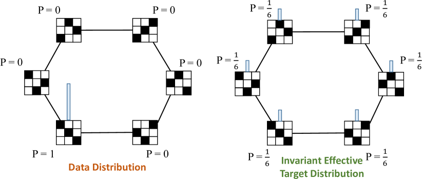
Figure 1: Empirical distribution and invariant effective target distribution of a $3\times 3$ binary adjacency matrix.

Figure 2: Recall curve.

Formally, given a training set of adjacency matrices $\{\boldsymbol{A}_{i}\}_{i=1}^{m}$, one can construct the union set of each graph’s isomorphism class, denoted as $\mathcal{A}^{*}=\mathcal{I}_{\boldsymbol{A}_{1}}\cup\mathcal{I}_{\boldsymbol{A}_{2}}\cdots\cup\mathcal{I}_{\boldsymbol{A}_{m}}$. The corresponding Dirac delta mixture distribution is $p_{\text{data}}^{*}(\boldsymbol{A})\coloneqq\frac{1}{Z}\sum_{\boldsymbol{A}^{*}\in\mathcal{A}^{*}}\delta(\boldsymbol{A}-\boldsymbol{A}^{*})$, where $Z=|\mathcal{A}^{*}|=O(n!m)$ is the normalizing constant. Note that $Z=n!m$ may not be achievable due to graph automorphism.

Lemma 3.1.

Let $\mathcal{P}$ denote all discrete permutation invariant distributions. The closest distributions in $\mathcal{P}$ to $p_{\text{data}}$, measured by total variation, have at least $\Omega(n!)$ modes. If, in addition, we restrict $\mathcal{P}$ to be the set of permutation invariant distributions such that $p(\boldsymbol{A}_{i})=p(\boldsymbol{A}_{j})>0$ for all matrices in the training set $\{\boldsymbol{A}_{l}\}_{l=1}^{m}$, then the closest distribution is given by $\operatorname*{arg\,min}_{q\in\mathcal{P}}TV(q,p_{\text{data}})=p_{\text{data}}^{*}$.

Under mild conditions, $p_{\text{data}}^{*}(\boldsymbol{A})$ of $O(n!m)$ modes becomes the effective target distribution, which is the case of the existing equivariant networks that learn invariant model distributions (see Appendix A for more details). In contrast, if we employ a non-equivariant network (i.e., the underlying model distribution is not invariant), the effective target distribution would be $p_{\text{data}}(\boldsymbol{A})$ which only has $O(m)$ modes. Arguably, learning a permutation invariant distribution is much harder than learning a non-invariant one, as the number of modes of the effective target distribution is often much higher.

Empirical Investigation. In the training data $\{\boldsymbol{A}_{i}\}_{i=1}^{m}$, we usually observe one adjacency matrix out of its isomorphism class. One can easily construct $p_{\text{data}}^{*}$ based on $p_{\text{data}}$ by applying permutation $n!$ times. We define a trade-off between them, dubbed the $k$-permuted empirical distribution: $p_{\text{data}}^{k}(\boldsymbol{A})\coloneqq\frac{1}{mk}\sum_{i=1}^{m}\sum_{j=1}^{k}\delta(\boldsymbol{A}-P_{j}\boldsymbol{A}_{i}P_{j}^{\top})$, where $P_{1},\ldots,P_{k}$ are $k$ distinct permutation matrices. $p_{\text{data}}^{k}$ has $O(km)$ modes, which is governed by $k$. With proper permutation matrices, $p_{\text{data}}^{k}=p_{\text{data}}$ when $k=1$ and $p_{\text{data}}^{k}\approx p_{\text{data}}^{*}$ when $k=n!$ (they are exactly the same if there is no non-trivial automorphisms).

Subsequently, we let the $k$-permuted distribution $p_{\text{data}}^{k}$ serve as the effective target distribution of a diffusion model and study the effect of $k$ (i.e., the number of modes in the effective target distribution) on the empirical performance. As discussed previously, an equivariant network matches the invariant target $p_{\text{data}}^{*}$ with $O(n!m)$ modes as in the case of $k=n!$. For $k<n!$, one must resort to the non-equivariant network that learns an non-invariant empirical distribution.

We conduct experiments on a toy dataset to assess empirical performance, where we ensure training is converged for all models. The dataset consists of 10 random regular graphs with degrees in $[2,11]$ and each of them has 16 nodes. The $k$ values are selected in the range of $[1,500]$. We use two equivariant networks as baselines to learn the invariant target $p_{\text{data}}^{*}$: DiGress [64] and PPGN [41]. Notably, the PPGN is a 3WL-discriminative GNN that entails rich expressiveness. For the non-equivariant networks matching $p_{\text{data}}^{k}$ with $k<n!$, we add index-based positional embedding to PPGN and compare it with our non-equivariant SwinGNN network (detailed in Sec. 4.1). We use the recall as the metric, defined by the proportion of generated graphs that are isomorphic to any training graph. The recall requires isomorphism testing and is invariant to permutation, which is fair for all models. Please see Sec. B.1 for more details on datasets and experiment setup.

As shown in Fig. 2, the permutation-invariant diffusion models DiGress and PPGN fail to achieve high recall. In contrast, the non-invariant models perform exceptionally well when $k$ is small, i.e., the target distributions have modest permutation data augmentation. As $k$ goes up, the sample quality of the non-invariant models drops significantly, indicating the learning difficulties incurred by more modes. Notably, the invariant diffusion models, whether employing discrete (DiGress) or continuous (PPGN) Markov chains, perform worse than the non-invariant models. We provide sample complexity analysis for the non-invariant models in Sec. A.4. Our empirical investigation shows that non-invariant models successfully match non-invariant target distributions, leading to stronger empirical performance. Building upon these findings, we present our novel non-invariant model, designed to produce graph data of exceptional quality.

4 Method

Motivated by the hardness results of learning permutation invariant models, we introduce SwinGNN, a novel non-invariant diffusion model that can generate large-scale graphs with high qualities.

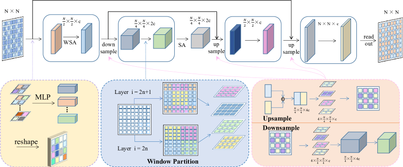
Figure 3: The overall architecture of our SwinGNN.

4.1 Efficient High-order Graph Transformer

A continuous denoising network for graph data takes a noisy adjacency matrix $\boldsymbol{\tilde{A}}$ and its noise level $\sigma$ as input and outputs a denoised adjacency matrix. Unlike in typical graph representation learning, our model does not have any graph topology (i.e., binary adjacency matrices) as input. We argue the interaction among edge representations (i.e., the noisy adjacency matrix entries) is critical. Each entry of the true score function $s(\boldsymbol{\tilde{A}})=\frac{\partial\log p_{\sigma}(\boldsymbol{\tilde{A}})}{\partial\boldsymbol{\tilde{A}}}$ depends on the whole input matrix $\boldsymbol{\tilde{A}}$. Therefore, the message passing mechanism must allow edge entries at different positions to interact with other.

To this end, we propose a graph transformer as the denoising network to better capture the edge-to-edge interplay. Our model treats each edge representation in the input matrix as a token, apply transformers with self-attention [62] to update the token representation, and output final edge representations for denoising. The rationale is similar to $k$-order GNN [42] or $k$-WL GNN [46] that improves network expressivity by using $k$-tuples of nodes ($k=2$ in our case). The $k$-WL discrimination power characterizes the isomorphism testing capability, which is equivalent to the function approximation capacity [6]. However, a naive extension of pure transformer results in poor scalability: for a graph with $n$ nodes, we have $O(n^{2})$ edge tokens, and the self-attention computation complexity is $O(n^{4})$.

Approximating Edge-to-Edge Attention. To reduce the computation complexity of the high-order graph transformer, we apply window-based partitioning to restrict self-attention to local representations. The model splits the $n\times n$ entries into local windows of size $M\times M$ in the grid map and computes self-attention for entries belonging to the same window in parallel. The number of tokens inside each window is $M^{2}$, and the self-attention complexity becomes $O(n^{2}M^{2})$, which is considerably smaller than the original $O(n^{4})$ with some reasonable $M$. The local self-attention window comes at the cost of blocking message passing between tokens belonging to different windows. To better model cross-window interactions, we adopt the shifted window technique [37] to create a non-regular partitioning window as shown in Fig. 3. We use regular and shifted window partitioning interchangeably to approximate the dense edge-to-edge interaction.

Multi-scale Edge Representation Learning. The window self-attention complexity $O(n^{2}M^{2})$ is dependent on $n^{2}$, which hinders scaling for large graphs. To further reduce memory footprint and better capture long-range interaction, we apply channel mixing-based downsampling and upsampling layers to construct hierarchical graph representations. As shown in Fig. 3, in the downsampling layer, we split the edge representation tensor into four half-sized tensors by index parity (odd or even) along rows and columns, make concatenation along channel dimension, and update tokens in the downsized tensors independently using an MLP. The upsampling stage is carried out likewise in the opposite direction, following the skip connection that concatenates same-size token tensors along channels.

Putting things together, we propose our model, dubbed SwinGNN, that efficiently learns edge-wise representations via approximating dense edge-to-edge interaction. Our proposed SwinGNN serves as a high-order graph transformer specifically designed to handle edge representations, distinguishing it from the vision SwinTransformer that learns image-level representations. Refer to Tab. 1 and  Sec. B.5 for experimental results showcasing our model’s superior performance.

4.2 Training and Sampling with SDE

We construct the noisy data distribution through stochastic differential equation (SDE) modeling with a continuous time variable $t\in[0,T]$. Let $\sigma$ evolve with $t$ and the noisy distribution reads as:

$$p_{\sigma(t)}(\boldsymbol{\tilde{A}})=\frac{1}{m}\sum_{i=1}^{m}\mathcal{N}(\boldsymbol{\tilde{A}};\boldsymbol{A}_{i},\sigma^{2}(t)\boldsymbol{I}),\boldsymbol{A}_{i}\in\mathcal{A}.$$ (3)

In other words, $p_{\sigma(0)}$ is the Dirac delta data distribution, and $p_{\sigma(T)}$ is close to the pure Gaussian noise (sampling prior distribution). The general forward and reverse process SDEs [58] are defined by:

(4)

(5)

where the $d\boldsymbol{A}_{+}$ and $d\boldsymbol{A}_{-}$ denote forward and reverse processes respectively, $f_{d}(\boldsymbol{A},t)$ and $g_{d}(t)$ are the drift and diffusion coefficients, and $\boldsymbol{W}$ is the standard Wiener process. We solve for the $f_{d}(\boldsymbol{A},t)$ and $g_{d}(t)$ so that the noisy distribution $p_{t}$ in Eq. 5 satisfies Eq. 3, and the solution is given by

$$f(\boldsymbol{A},t)=\boldsymbol{0},g(t)=\sqrt{2\dot{\sigma}(t)\sigma(t)},$$

which can be found in Eq. (9) of [58] or Eq. (6) of [27].

Noise Scheduling and Network Preconditioning. We select the time-varying noise strength $\sigma(t)$ to be linear with $t$, i.e., $\sigma(t)=t$, as in [47, 56], which turns the SDEs into

$$d\boldsymbol{A}_{+}=\sqrt{2t}d\boldsymbol{W},d\boldsymbol{A}_{-}=-2t\nabla_{\boldsymbol{A}}\log p_{t}(\boldsymbol{A})dt+\sqrt{2t}d\boldsymbol{W}.$$ (6)

Moreover, we adopt network preconditioning for improved training dynamics following the Elucidating Diffusion Model (EDM) [27]. First, instead of training DSM with Eq. 2, we use its equivalent form in Eq. (1), and parameterize denoising function $D_{\theta}$ with noise (time) dependent scaling: $D_{\theta}(\boldsymbol{\tilde{A}},\sigma)=c_{s}(\sigma)\boldsymbol{\tilde{A}}+c_{o}(\sigma)F_{\theta}(c_{i}(\sigma)\boldsymbol{\tilde{A}},c_{n}(\sigma)),$ where $F_{\theta}$ is the actual neural network and the other coefficients are summarized in Sec. B.4. During implementation, $D_{\theta}$ is a wrapper with preconditioning operations, and we construct $F_{\theta}$ using our SwinGNN model in Sec. 4.1. Second, we sample $\sigma$ with $\ln(\sigma)\sim\mathcal{N}(P_{\text{mean}},P_{\text{std}}^{2})$ to select noise (time) stochastically in a broad range to draw training samples. Third, we apply the weighting coefficients $\lambda(\sigma)=1/c_{o}(\sigma)^{2}$ on the denoising objective to improve training stability. The overall training objective is

$$\mathbb{E}_{\sigma,\boldsymbol{A},\boldsymbol{\tilde{A}}}\left[\lambda(\sigma)\|c_{s}(\sigma)\boldsymbol{\tilde{A}}+c_{o}(\sigma)F_{\theta}(c_{i}(\sigma)\boldsymbol{\tilde{A}},c_{n}(\sigma))-\boldsymbol{A}\|^{2}_{F}\right].$$ (7)

The target of $F_{\theta}$ is $\frac{\boldsymbol{A}-c_{s}(\sigma)\boldsymbol{\tilde{A}}}{c_{o}(\sigma)}$, an interpolation between pure Gaussian noise $\boldsymbol{A}-\boldsymbol{\tilde{A}}$ (when $\sigma\rightarrow 0$) and clean sample $\boldsymbol{A}$ (when $\sigma\rightarrow\infty$), downscaled by $c_{o}(\sigma)$. These measures altogether ease the training of $F_{\theta}$ by making the network inputs and targets have unit variance.

Self-Conditioning. We also apply self-conditioning [5] to let $D_{\theta}$ dependent on the sample created by itself. We change the denoising function to be $D_{\theta}(\boldsymbol{\tilde{A}},\boldsymbol{\hat{A}},\sigma)$ (likewise $F_{\theta}(\boldsymbol{\tilde{A}},\boldsymbol{\hat{A}},\sigma)$), where $\boldsymbol{\hat{A}}$ is a sample previously created by $D_{\theta}$. In the reverse process, $D_{\theta}$ iteratively denoises corrupted samples, and it can access generated sample $\boldsymbol{\hat{A}}$ after the first step. This is implemented by concatenating $\boldsymbol{\tilde{A}}$ and $\boldsymbol{\hat{A}}$ at the first layer of $F_{\theta}$. During training, given a noisy sample $\boldsymbol{\tilde{A}}$, with 50% probability, we set $\boldsymbol{\hat{A}}=\boldsymbol{0}$; otherwise, we first obtain $\boldsymbol{\hat{A}}=D_{\theta}(\boldsymbol{\tilde{A}},\boldsymbol{0},\sigma)$, and then use it as the self-conditioning signal. Note we disable the gradient calculation w.r.t. $\boldsymbol{\hat{A}}$, so the extra memory overhead is negligible.

Stochastic Sampler with 2${}^{\text{nd}}$-order Correction. Our sampler is formally presented in Alg. 1. It is based on the 2${}^{\text{nd}}$-order sampler in [27]. At the $i$-th iteration, the sampler adds noise to $\boldsymbol{\widetilde{A}}^{(i)}$ moving slightly forward to time $\hat{t}_{i}$, evaluate $d\boldsymbol{A}/dt$ at $\hat{t}_{i}$, and moves backward following the reverse process in Eq. 6 to obtain $\boldsymbol{\widetilde{A}}^{(i+1)}$. The sampler then evaluates $d\boldsymbol{A}/dt$ on time $t_{i+1}$ and corrects for $\boldsymbol{\widetilde{A}}^{(i+1)}$ using Heun’s integration [61]. Also, we keep track of the generated samples $\boldsymbol{\widehat{A}}^{(i)}_{\text{sc}}$ for model self-conditioning. We investigate the effects of the above modeling techniques in Tab. 3.

4.3 Permutation Invariant Sampling

Algorithm 1 Sampler w. 2${}^{\text{nd}}$-order correction.

0:  $D_{\theta},N,\{t_{i}\}_{i=0}^{N},\{\gamma_{i}\}_{i=0}^{N-1}.$

1:  sample $\small\boldsymbol{\widetilde{A}}^{(0)}\sim\mathcal{N}(\boldsymbol{0},t_{0}^{2}\boldsymbol{I}),\boldsymbol{\widehat{A}}^{(0)}_{\text{sc}}=\boldsymbol{0}$.

2:  for $i=0$ to $N-1$ do

3:     sample $\small\boldsymbol{\epsilon}\sim\mathcal{N}(\boldsymbol{0},S_{\text{noise}}^{2}\boldsymbol{I})$

4:     $\small\hat{t}_{i}\leftarrow(1+\gamma_{i})t_{i}$

5:     $\small\boldsymbol{\widetilde{A}}^{(\hat{i})}\leftarrow\boldsymbol{\widetilde{A}}^{(i)}+\sqrt{\hat{t}_{i}^{2}-t_{i}^{2}}\boldsymbol{\epsilon}$

6:     $\small\boldsymbol{\widehat{A}}^{(\hat{i})}_{\text{sc}}\leftarrow D_{\theta}(\boldsymbol{\widetilde{A}}^{(\hat{i})},\boldsymbol{\widehat{A}}^{(i)}_{\text{sc}},\hat{t}_{i})$

7:     $\small\boldsymbol{d}_{i}\leftarrow(\boldsymbol{\widetilde{A}}^{(\hat{i})}-\boldsymbol{\widehat{A}}^{({\hat{i}})}_{\text{sc}})/\hat{t}_{i}$

8:     $\small\boldsymbol{\widetilde{A}}^{(i+1)}\leftarrow\boldsymbol{\widetilde{A}}^{(\hat{i})}+(t_{i+1}-\hat{t}_{i})\boldsymbol{d}_{i}$ # Below is 2${}^{\text{nd}}$-order correction.

9:     $\small\boldsymbol{\widehat{A}}^{(i+1)}_{\text{sc}}\leftarrow D_{\theta}(\boldsymbol{\widetilde{A}}^{(i+1)},\boldsymbol{\widehat{A}}^{({\hat{i}})}_{\text{sc}},{t}_{i+1})$

10:     $\small\boldsymbol{d}_{i}^{\prime}\leftarrow(\boldsymbol{\widetilde{A}}^{(i+1)}-\boldsymbol{\widehat{A}}^{(i+1)}_{\text{sc}})/{t}_{i+1}$

11:     $\small\boldsymbol{\widetilde{A}}^{(i+1)}\leftarrow\boldsymbol{\widetilde{A}}^{(i)}+\frac{1}{2}(t_{i+1}-\hat{t}_{i})(\boldsymbol{d}_{i}+\boldsymbol{d}_{i}^{\prime})$

12:  end for

13:  return $\boldsymbol{\widetilde{A}}^{(N)}$

Finally, we present a simple trick to achieve permutation invariance during sampling. Let $\boldsymbol{A}\sim p_{\theta}(\boldsymbol{A})$ be a random adjacency matrix drawn from the model distribution following Alg. 1. As our architecture does not preserve permutation equivariance, $p_{\theta}$ is not permutation invariant, i.e., $p_{\theta}(\boldsymbol{A})=p_{\theta}(P\boldsymbol{A}P^{\top}),\forall P\in\mathcal{S}_{n}$ is not guaranteed. We have the following lemma to construct a permutation invariant sampling distribution.

Lemma 4.1.

Let $\boldsymbol{A}$ be a random adjacency matrix distributed according to any graph distribution on $n$ vertices. Let $P_{r}\sim\mathrm{Unif}(\mathcal{S}_{n})$ be uniform over the set of permutation matrices. Then, the induced distribution of the random matrix $\boldsymbol{A}_{r}=P_{r}\boldsymbol{A}P_{r}^{\top}$, denoted as $q_{\theta}(\boldsymbol{A}_{r})$, is permutation invariant, i.e., $q_{\theta}(\boldsymbol{A}_{r})=q_{\theta}(P\boldsymbol{A}_{r}P^{\top}),\forall P\in\mathcal{S}_{n}$.

This trick is applicable to all types of generative models. Note that the random permutation does not go beyond the isomorphism class. Although $q_{\theta}$ is invariant, it captures the same amount of isomorphism classes as $p_{\theta}$. Graphs generated from $q_{\theta}$ must have isomorphic counterparts that $p_{\theta}$ could generate.

5 Experiments

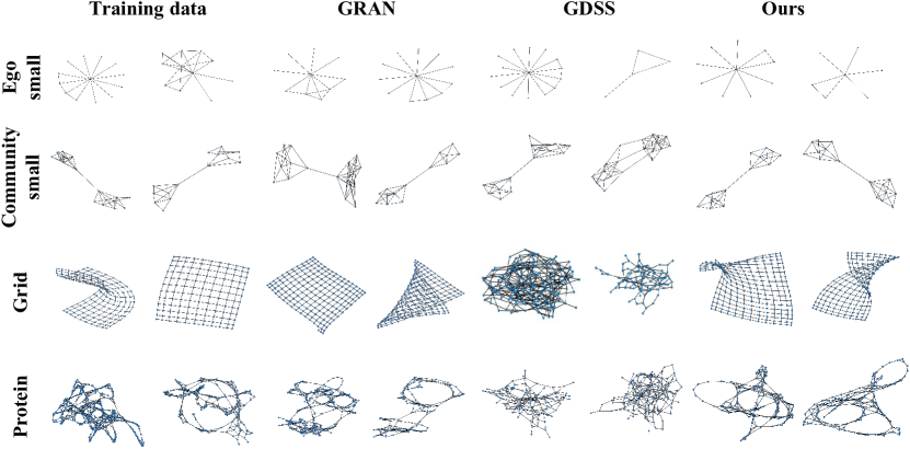
Figure 4: Sample graphs generated by different models.

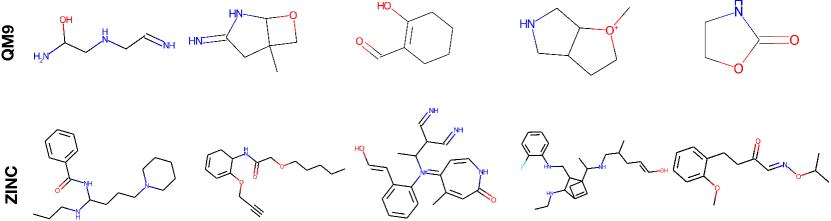
Figure 5: Molecules generated by our models.

We now empirically verify the effectiveness of our model on synthetic and real-world graph datasets including molecule generation with node and edge attributes.

Experiment Setup. We consider the following synthetic and real-world graph datasets: (1) Ego-small: 200 small ego graphs from Citeseer dataset [51], (2) Community-small: 100 random graphs generated by Erdős–Rényi model [13] consisting of two equal-sized communities, (3) Grid: 100 random 2D grid graphs with $|\mathcal{V}|\in[100,400]$, (4) DD protein dataset [11], (5) QM9 dataset [50], (6) ZINC250k dataset [22]. Please see Appendix B for more details on datasets and evaluation protocols.

Baselines. We compare our method with state-of-the-art graph generative models. For non-molecule experiments, we include autoregressive model GRAN [34], VAE-base GraphVAE-MM [72] and GAN-based SPECTRE [43] as baselines. We also compare with continuous diffusion models with permutation equivariant backbone, i.e., EDP-GNN [48] and GDSS [24], and discrete diffusion model DiGress [64]. We additionally compare to the PPGN networks used in Sec. 3.2. Moreover, to validate the effectiveness of our SwinGNN, we also compare it with a recent UNet [10] and the vision SwinTransformer [37] backbones. Specifically, we employ the UperNet on top of the SwinTransformer for the denoising task (refer to Sec. B.5 for more details). We re-run all these baselines with the same data split for a fair comparison. For molecule generation, we compare with GDSS [24], DiGress [64], GraphAF [53] and GraphDF [38].

Implementation Details. Besides molecule generation, we try two variants of our SwinGNN: standard SwinGNN with 60-dim token and large SwinGNN-L with 96-dim token. For molecule generation, we compare different ways to encode node and edge attributes using scalar, binary bits or one-hot encoding. The same training and sampling methods as in Sec. 4.2 are used for the UNet baseline. We use self-conditioning and exponential moving average (EMA) to train SwinGNN variants in all experiments. We leave more implementation details in Appendix B.

	Ego-Small			Community-Small			Grid			Protein
Methods	Deg. $\downarrow$	Clus. $\downarrow$	Orbit. $\downarrow$	Deg. $\downarrow$	Clus. $\downarrow$	Orbit. $\downarrow$	Deg. $\downarrow$	Clus. $\downarrow$	Orbit. $\downarrow$	Deg. $\downarrow$	Clus. $\downarrow$	Orbit. $\downarrow$
GRAN	3.40e-3	2.83e-2	1.16e-2	4.00e-3	1.44e-1	4.10e-2	8.23e-4	3.79e-3	1.59e-3	6.40e-3	6.03e-2	2.02e-1
EDP-GNN	1.12e-2	2.73e-2	1.12e-2	1.77e-2	7.23e-2	6.90e-3	9.15e-1	3.78e-2	1.15	9.50e-1	1.63	8.37e-1
GDSS	2.59e-2	8.91e-2	1.38e-2	3.73e-2	7.02e-2	6.60e-3	3.78e-1	1.01e-2	4.42e-1	1.11	1.70	0.27
DiGress	1.20e-1	1.86e-1	3.48e-2	8.99e-2	1.92e-1	7.48e-1	9.57e-1	2.66e-2	1.03	8.31e-2	2.60e-1	1.17e-1
GraphVAE-MM	3.45e-2	7.32e-1	6.39e-1	5.87e-2	3.56e-1	5.32e-2	5.90e-4	0.00	1.60e-3	7.95e-3	6.33e-2	9.24e-2
SPECTRE	4.61e-2	1.30e-1	6.58e-3	8.65e-3	7.06e-2	8.18e-3	-	-	-	-	-	-
PPGN	2.37e-3	3.77e-2	4.71e-3	1.14e-2	1.74e-1	4.15e-2	1.77e-1	1.47e-3	1.52e-1	-	-	-
PPGN+PE	1.21e-3	3.76e-2	4.94e-3	2.20e-3	9.37e-2	3.76e-2	8.48e-2	5.37e-2	7.94e-3	-	-	-
SwinTF	8.50e-3	4.42e-2	8.00e-3	2.70e-3	7.11e-2	1.30e-3	2.50e-3	8.78e-5	1.25e-2	4.99e-2	1.32e-1	1.56e-1
UNet	9.38e-4	2.79e-2	6.08e-3	4.29e-3	7.24e-2	8.33e-3	9.35e-6	0.00	6.91e-5	5.48e-2	7.26e-2	2.71e-1
SwinGNN	3.61e-4	2.12e-2	3.58e-3	2.98e-3	5.11e-2	4.33e-3	1.91e-7	0.00	6.88e-6	1.88e-3	1.55e-2	2.54e-3
SwinGNN-L	5.72e-3	3.20e-2	5.35e-3	1.42e-3	4.52e-2	6.30e-3	2.09e-6	0.00	9.70e-7	1.19e-3	1.57e-2	8.60e-4

Table 1: Quantitative results on ego-small, community-small, grid, and protein benchmark datasets. Dash means out of compute when running experiments.

	QM9				ZINC250k
Methods	Valid w/o cor.$\uparrow$	Unique$\uparrow$	FCD$\downarrow$	NSPDK$\downarrow$	Valid w/o cor.$\uparrow$	Unique$\uparrow$	FCD$\downarrow$	NSPDK$\downarrow$
GraphAF	57.16	83.78	5.384	2.10e-2	68.47	99.01	16.023	4.40e-2
GraphDF	79.33	95.73	11.283	7.50e-2	41.84	93.75	40.51	3.54e-1
GDSS	90.36	94.70	2.923	4.40e-3	97.35	99.76	11.398	1.80e-2
DiGress	95.43	93.78	0.643	7.28e-4	84.94	99.21	4.88	8.75e-3
SwinGNN (scalar)	99.68	95.92	0.169	4.02e-4	87.74	99.98	5.219	7.52e-3
SwinGNN (bits)	99.91	96.29	0.142	3.44e-4	83.50	99.97	4.536	5.61e-3
SwinGNN (one-hot)	99.71	96.25	0.125	3.21e-4	81.72	99.98	5.920	6.98e-3
SwinGNN-L (scalar)	99.88	96.46	0.123	2.70e-4	93.34	99.80	2.492	3.60e-3
SwinGNN-L (bits)	99.97	95.88	0.096	2.01e-4	90.46	99.79	2.314	2.36e-3
SwinGNN-L (one-hot)	99.92	96.02	0.100	2.04e-4	90.68	99.73	1.991	1.64e-3

Table 2: Quantitative results on QM9 and ZINC250k molecule datasets. Baseline results are reproduced by us using a consistent experimental protocol.

5.1 Synthetic Datasets

Fig. 4 showcases samples generated by various models on ego-small, community-small, and grid datasets. The quality of our generated samples is high and comparable to that of auto-regressive models. Equivariant diffusion models like GDSS can capture structural information for small graphs but fail on larger and more complicated graphs (e.g., grid). Quantitative maximum mean discrepancy (MMD) results are presented in Tab. 1. Our SwinGNN consistently outperforms the baselines across all datasets by several orders of magnitude, and can generate large graphs with around 500 nodes (grid). Notably, our tailored SwinGNN backbone exhibits superior performance compared to UNet.

5.2 Real-world Datasets

Protein Dataset.

We conduct experiments on the DD protein dataset. As shown in Fig. 4, our model can generate samples visually similar to those from the dataset, while previous diffusion models cannot learn the topology well. Tab. 1 demonstrates that the MMD metrics of our model surpass the baselines by several orders of magnitude.

Molecule Datasets.

Our SwinGNN generates molecule graphs with node and edge features, and the details for extending SwinGNN for such tasks are provided in Sec. B.3. We evaluate our model against baselines on QM9 and ZINC250k using metrics such as validity without correction, uniqueness, Fréchet ChemNet Distance (FCD) [49], and neighborhood subgraph pairwise distance kernel (NSPDK) MMD [8]. Notably, our models exhibit substantial improvements in FCD and NSPDK metrics, surpassing the baselines by several orders of magnitude.

5.3 Ablation Study

			Grid
Method	Self-cond.	EMA	Deg. $\downarrow$	Clus. $\downarrow$	Orbit. $\downarrow$
EDM	✓	✓	1.91e-7	0.00	6.88e-6
EDM	✗	✓	1.14e-5	2.15e-5	1.58e-5
EDM	✓	✗	5.12e-5	2.43e-5	3.38e-5
EDM	✗	✗	5.90e-5	2.71e-5	9.24e-5
DDPM	✓	✓	2.89e-3	1.36e-4	3.70e-3
DDPM	✗	✗	4.01e-2	8.62e-2	1.05e-1

Table 3: Ablation results on grid dataset.

We perform ablations on grid dataset to validate the techniques in Sec. 4.2. Following EDM [27], we incorporate SDE modeling and adopt the objective in Eq. 7, which we compare against the vanilla DDPM [18]. The EDM framework provides a significant boost in performance. Also, EMA consistently improves the model regardless of other techniques, but is limited compared to EDM. Self-conditioning [5] contributes minimally on its own. Nevertheless, when combined with EMA, it improves the model significantly and enables the model to achieve its best results.

6 Conclusion

We investigate the hardness of learning permutation invariant denoising diffusion graph generative models from theoretical and empirical perspectives, attributed to the multi-modal effective target distribution. We propose a non-invariant SwinGNN that efficiently performs edge-to-edge message passing and can generate large graphs with high qualities. Experiments show that our model achieves state-of-the-art performance in a wide range of datasets. In the future, it is promising to generalize our model to the discrete denoising diffusion framework which is more memory efficient.

Appendix A Proofs and Additional Theoretical Analysis

A.1 Proof of Lemma 3.1

See 3.1

Figure A.1: Different configurations of $TV(q,p_{\text{data}})$, given fixed $\mathcal{A}$ (the support of $p_{\text{data}}$) and its induced $\mathcal{A}^{*}$. Here, we modify $\mathcal{Q}$ (the support of $q$). Left: maximal TV, $\mathcal{Q}$ is disjoint from $\mathcal{A}/\mathcal{A}^{*}$. Middle: intermediate TV, intersecting $\mathcal{Q}$ and $\mathcal{A}/\mathcal{A}^{*}$. Right: minimal TV, $\mathcal{Q}=\mathcal{A}^{*}$.

Proof.

Recall the definitions on $p_{\text{data}}$ and $p_{\text{data}}^{*}$ in our context:

$$p_{\text{data}}(\boldsymbol{A})=\frac{1}{m}\sum_{i=1}^{m}\delta(\boldsymbol{A}-\boldsymbol{A}_{i}),p_{\text{data}}^{*}(\boldsymbol{A})=\frac{1}{Z}\sum_{\boldsymbol{A}^{*}_{i}\in\mathcal{A}^{*}}\delta(\boldsymbol{A}-\boldsymbol{A}^{*}_{i})$$

In other words, $p_{\text{data}}$ and $p_{\text{data}}^{*}$ are both discrete uniform distributions. We use $\mathcal{A}$ and $\mathcal{A}^{*}=\mathcal{I}_{\boldsymbol{A}_{1}}\cup\mathcal{I}_{\boldsymbol{A}_{2}}\cdots\cup\mathcal{I}_{\boldsymbol{A}_{m}}$ to denote the support of $p_{\text{data}}$ and $p_{\text{data}}^{*}$ respectively. Let $TV^{*}\coloneqq TV(p_{\text{data}}^{*},p_{\text{data}})$ be the “golden standard” total variation distance that we aim to outperform.

Let $q\in\mathcal{P}$ without loss of generality. As $q$ is permutation invariant, it must assign equal probability to graphs in the same isomorphism class. We denote the support of $q$ by $\mathcal{Q}=\{\mathcal{I}_{q_{i}}\}_{i=1}^{\Phi}$. $q(\boldsymbol{A})=\sum_{i=1}^{\Phi}\rho_{i}\sum_{\boldsymbol{A}_{i}\in\mathcal{I}_{q_{i}}}\delta(\boldsymbol{A}-\boldsymbol{A}_{i})$, where $\sum_{i=1}^{\Phi}\rho_{i}|\mathcal{I}_{q_{i}}|=1,\rho_{i}>0$, and $\Phi>0$ stand for the number of isomorphism classes contained in $q$. Fig. A.1 summarizes the possibilities of TV used in our proof.

Proof of $\Omega(n!)$ Modes. This first part of the lemma imposes no constraints on $\mathcal{P}$: we do not require distributions in $\mathcal{P}$ to be uniform on $\mathcal{A}$. We first prove two helpful claims and then use proof by contradiction to prove our result on $\Omega(n!)$ modes.

Claim 1: The maximal $TV(q,p_{\text{data}})$ is achieved when $\mathcal{Q}$ and $\mathcal{A}^{*}$ are disjoint (so are $\mathcal{Q}$ and $\mathcal{A}$).

Proof of Claim 1: Without loss of generality, the TV distance is:

$$TV(q,p_{\text{data}}) =\sum_{i=1}^{\Phi}\left(\sum_{\boldsymbol{A}\in\mathcal{I}_{q_{i}}\cap\mathcal{A}}\left|\rho_{i}-\frac{1}{|\mathcal{A}|}\right|+\sum_{\boldsymbol{A}\in\mathcal{I}_{q_{i}},\boldsymbol{A}\notin\mathcal{A}}\rho_{i}\right)+\sum_{\boldsymbol{A}\notin\mathcal{Q},\boldsymbol{A}\in\mathcal{A}}\frac{1}{|\mathcal{A}|}$$

$$<\sum_{i=1}^{\Phi}\left(\sum_{\boldsymbol{A}\in\mathcal{I}_{q_{i}}\cap\mathcal{A}}(\rho_{i}+\frac{1}{|\mathcal{A}|})+\sum_{\boldsymbol{A}\in\mathcal{I}_{q_{i}},\boldsymbol{A}\notin\mathcal{A}}\rho_{i}\right)+\sum_{\boldsymbol{A}\notin\mathcal{Q},\boldsymbol{A}\in\mathcal{A}}\frac{1}{|\mathcal{A}|}$$ (triangle inequality)

$$=\sum_{i=1}^{\Phi}\left(\sum_{\boldsymbol{A}\in\mathcal{I}_{q_{i}}\cap\mathcal{A}}\frac{1}{|\mathcal{A}|}+\sum_{\boldsymbol{A}\in\mathcal{I}_{q_{i}}}\rho_{i}\right)+\sum_{\boldsymbol{A}\notin\mathcal{Q},\boldsymbol{A}\in\mathcal{A}}\frac{1}{|\mathcal{A}|}$$

$$=\sum_{i=1}^{\Phi}\sum_{\boldsymbol{A}\in\mathcal{I}_{q_{i}}}\rho_{i}+\sum_{\boldsymbol{A}\in\mathcal{A}}\frac{1}{|\mathcal{A}|}=2$$

The triangle inequality is strict as $\rho_{i}$ and $\frac{1}{|\mathcal{A}|}$ are both strictly positive, and $|\rho_{i}-\frac{1}{|\mathcal{A}|}|<\rho_{i}+\frac{1}{|\mathcal{A}|}$ always holds. Namely, $TV(q,p_{\text{data}})$ is bounded by 2. If $\mathcal{Q}$ and $\mathcal{A}^{*}$ are disjoint, $TV(q,p_{\text{data}})=\sum_{i=1}^{\Phi}\frac{1}{|\mathcal{I}_{q_{i}}|}\times\rho_{i}+\frac{1}{|\mathcal{A}|}\times|\mathcal{A}|=2,$ meaning that the maximum TV distance is achieved when there is no intersection between $\mathcal{Q}$ and $\mathcal{A}^{*}$.

Claim 2: It is always possible to have a $q\in\mathcal{P}$ with $TV(q,p_{\text{data}})<2$ by allowing $\mathcal{Q}$ and $\mathcal{A}^{*}$ to intersect on some isomorphism classes $\{\mathcal{I}_{q_{i}}\}_{i\in\nu}$. Notice $\mathcal{I}_{q_{i}}\cap\mathcal{A}\neq\emptyset,\forall i\in\nu$ as per isomorphism.

Proof of Claim 2:

$$TV(q,p_{\text{data}}) =\sum_{i=1}^{\Phi}\left(\sum_{\boldsymbol{A}\in\mathcal{I}_{q_{i}}\cap\mathcal{A}}\left|\rho_{i}-\frac{1}{|\mathcal{A}|}\right|+\sum_{\boldsymbol{A}\in\mathcal{I}_{q_{i}},\boldsymbol{A}\notin\mathcal{A}}\rho_{i}\right)+\sum_{\boldsymbol{A}\notin\mathcal{Q},\boldsymbol{A}\in\mathcal{A}}\frac{1}{|\mathcal{A}|}$$

$$=\sum_{i\in\nu}\left(\sum_{\boldsymbol{A}\in\mathcal{I}_{q_{i}}\cap\mathcal{A}}\left|\rho_{i}-\frac{1}{|\mathcal{A}|}\right|+\sum_{\boldsymbol{A}\in\mathcal{I}_{q_{i}},\boldsymbol{A}\notin\mathcal{A}}\rho_{i}\right)+\sum_{i\notin\nu}\sum_{\boldsymbol{A}\in\mathcal{I}_{q_{i}}}\rho_{i}+\sum_{\boldsymbol{A}\notin\mathcal{Q},\boldsymbol{A}\in\mathcal{A}}\frac{1}{|\mathcal{A}|}$$

$$=\sum_{i\in\nu}\left(|\mathcal{I}_{q_{i}}\cap\mathcal{A}|\left|\rho_{i}-\frac{1}{|\mathcal{A}|}\right|+(\mathcal{I}_{q_{i}}-|\mathcal{I}_{q_{i}}\cap\mathcal{A}|)\rho_{i}\right)+\sum_{i\notin\nu}\rho_{i}|\mathcal{I}_{q_{i}}|+\sum_{\boldsymbol{A}\notin\mathcal{Q},\boldsymbol{A}\in\mathcal{A}}\frac{1}{|\mathcal{A}|}$$

$$=\sum_{i\in\nu}|\mathcal{I}_{q_{i}}\cap\mathcal{A}|\left(\left|\rho_{i}-\frac{1}{|\mathcal{A}|}\right|-\rho_{i}\right)+\overbrace{\sum_{i=1}^{\Phi}\rho_{i}|\mathcal{I}_{q_{i}}|}^{1}+\overbrace{\sum_{\boldsymbol{A}\in\mathcal{A}}\frac{1}{|\mathcal{A}|}}^{1}-\sum_{\boldsymbol{A}\in\mathcal{Q}\cap\mathcal{A}}\frac{1}{|\mathcal{A}|}$$

$$=\sum_{i\in\nu}|\mathcal{I}_{q_{i}}\cap\mathcal{A}|\left(\left|\rho_{i}-\frac{1}{|\mathcal{A}|}\right|-\rho_{i}\right)-\sum_{i=1}^{\Phi}|\mathcal{I}_{q_{i}}\cap\mathcal{A}|\frac{1}{|\mathcal{A}|}+2$$

$$=\sum_{i\in\nu}|\mathcal{I}_{q_{i}}\cap\mathcal{A}|\overbrace{\left(\left|\rho_{i}-\frac{1}{|\mathcal{A}|}\right|-\rho_{i}-\frac{1}{|\mathcal{A}|}\right)}^{<0}-\sum_{i\notin\nu}\overbrace{|\mathcal{I}_{q_{i}}\cap\mathcal{A}|\frac{1}{|\mathcal{A}|}}^{>0}+2$$

$$<2$$

The last inequality is strict as $\rho_{i}$, $\frac{1}{|\mathcal{A}|}$ and $|\mathcal{I}_{q_{i}}\cap\mathcal{A}|$ are all strictly positive for $i\in\nu$.

Claim 3: Let $q^{*}\in\operatorname*{arg\,min}_{q\in\mathcal{P}}TV(q,p_{\text{data}})$ be a minizizer whose support is $\mathcal{Q}^{*}$. $\mathcal{Q}^{*}$ and $\mathcal{A}^{*}$ must not be disjoint, i.e., $\mathcal{Q}^{*}$ intersects $\mathcal{A}^{*}$ for at least one isomorphism class in $\mathcal{A}^{*}$.

Proof of Claim 3: Assume $\mathcal{Q}^{*}$ and $\mathcal{A}^{*}$ have no intersection, then $\min_{q\in\mathcal{P}}TV(q,p_{\text{data}})=TV(q^{*},p_{\text{data}})=2$, which is validated in Claim 1. From Claim 2, we know there must exist another $q^{\dagger}\in\mathcal{P}$ with $TV(q^{\dagger},p_{\text{data}})<2.$ Therefore, $\min_{q\in\mathcal{P}}TV(q,p_{\text{data}})\leq TV(q^{\dagger},p_{\text{data}})<2$, which contradicts $\min_{q\in\mathcal{P}}TV(q,p_{\text{data}})=2$.

From Claim 3, we know the support of optimum $q^{*}$ must contain at least one isomorphism class in $\mathcal{A}^{*}$, whose size is up to $O(n!)$. Namely, $|\mathcal{Q}^{*}|$ has a lower bound $\Omega(n!)$ that does not depend on the size of empirical data distribution $|\mathcal{A}|$.

Proof of Optimality of $p_{\text{data}}^{*}$ when $\mathcal{P}$ is Discrete Uniform on a Superset of $\mathcal{A}$.

Now we proceed to prove the second part of our lemma, which is a special case when $\mathcal{P}$ has some constraints w.r.t. $\mathcal{A}$. Assume $\mathcal{A}=\{\boldsymbol{A}_{i}\}_{i=1}^{m}$ consists of $m$ graphs (adjacency matrices) belonging to $k$ isomorphic equivalence classes, where $m\geq k$ due to some potential isomorphic graphs. Subsequently, let $\mathcal{A}^{*}$ have $l$ adjacency matrices for all $k$ equivalence classes ($l\geq m$), i.e., $\mathcal{A}^{*}=\cup_{i=1}^{m}\mathcal{I}_{\boldsymbol{A}_{i}}=\cup_{i=1}^{k}\mathcal{I}_{c_{i}}$, where $\{\mathcal{I}_{c_{i}}\}_{i=1}^{k}$ denote $k$ equivalence classes.

Further, let $q_{\gamma}\in\mathcal{P}$ and let $\mathcal{Q}_{\gamma}\supseteq\mathcal{A}$ be its support. That is, $q_{\gamma}=\frac{1}{|\mathcal{Q}_{\gamma}|}\sum_{\boldsymbol{A}_{i}\in\mathcal{Q}_{\gamma}}\delta(\boldsymbol{A}-\boldsymbol{A}_{i}),$ where $|\mathcal{Q}_{\gamma}|\geq m$. The total variation distance is:

$$TV^{*} =|\frac{1}{m}-\frac{1}{l}|\times m+\frac{1}{l}(l-m)=2(1-\frac{m}{l}),$$

$$TV(q_{\gamma},p_{\text{data}}) =\left|\frac{1}{|\mathcal{Q}_{\gamma}|}-\frac{1}{m}\right|\times m+\left|\frac{|\mathcal{Q}_{\gamma}|-m}{|\mathcal{Q}_{\gamma}|}\right|=2\left(1-\frac{m}{|\mathcal{Q}_{\gamma}|}\right).$$

To minimize $TV(q_{\gamma},p_{\text{data}})$ over $q_{\gamma}$, we need to minimize $|\mathcal{Q}_{\gamma}|$. Since $\mathcal{A}\subseteq\mathcal{Q}_{\gamma}$ and $q_{\gamma}$ is permutation invariant, the smallest $|\mathcal{Q}_{\gamma}|$ would be $|\cup_{i=1}^{m}\mathcal{I}_{\boldsymbol{A}_{i}}|=|\cup_{i=1}^{k}\mathcal{I}_{c_{i}}|=|\mathcal{A}^{*}|=l$ . Therefore, we conclude that $\min\limits_{q_{\gamma}\in\mathcal{P}}TV(q_{\gamma},p_{\text{data}})=TV^{*}=2(1-\frac{m}{l}),$ and $\operatorname*{arg\,min}\limits_{q_{\gamma}\in\mathcal{P}}TV(q_{\gamma},p_{\text{data}})=p_{\text{data}}^{*}.$

Justification on the Constraints of $\mathcal{P}$ to Guarantee the Optimality of $p_{\text{data}}^{*}$.

In the end, we justify the reason why $\mathcal{P}$ has to be discrete uniform on a superset of $\mathcal{A}$ (i.e., assign equal probability to each element in $\mathcal{A}$) for the second part of the lemma to hold. We list all possible conditions in the table below and give concrete counterexamples for the cases where the optimality of $p_{\text{data}}^{*}$ is no longer true, i.e., $p_{\text{data}}^{*}\notin\operatorname*{arg\,min}\limits_{q\in\mathcal{P}}TV(q,p_{\text{data}})$ or equivalently $\min\limits_{q\in\mathcal{P}}TV(q,p_{\text{data}})<TV^{*}=TV(p_{\text{data}}^{*},p_{\text{data}}).$ For ease of proof, we further divide $p_{\text{data}}$ into two categories based on the existence of isomorphic graphs.

		$p_{\text{data}}$ conditions
		$\mathcal{A}$ has isomorphic graphs	$\mathcal{A}$ does not have isomorphic graphs
$\mathcal{P}$ conditions	support contains $\mathcal{A}$ and uniform	Our proof in the above: True, $\min\limits_{q\in\mathcal{P}}TV(q,p_{\text{data}})=TV^{*}$
	support contains $\mathcal{A}$ and not uniform	False, Case 1: $\min\limits_{q\in\mathcal{P}}TV(q,p_{\text{data}})<TV^{*}$	False, Case 2: $\min\limits_{q\in\mathcal{P}}TV(q,p_{\text{data}})<TV^{*}$
	support does not contain $\mathcal{A}$	False, Case 3: $\min\limits_{q\in\mathcal{P}}TV(q,p_{\text{data}})<TV^{*}$	False, Case 4: $\min\limits_{q\in\mathcal{P}}TV(q,p_{\text{data}})<TV^{*}$

Consider graphs with $n=4$ nodes, let the support of $p_{\text{data}}^{*}$ (i.e., $\mathcal{A}^{*}$) be adjacency matrices belonging to two isomorphism classes $\mathcal{I}_{a}$ and $\mathcal{I}_{b}$, where $|\mathcal{I}_{a}|=24$, $|\mathcal{I}_{b}|=6$. Namely, $\mathcal{I}_{a}$ has no automorphism (e.g., complete disconnected graphs), and the automorphism number of $\mathcal{I}_{b}$ is 4 (e.g., star graphs). Let $\mathcal{I}_{a}\coloneqq\{\boldsymbol{A}_{1},\boldsymbol{A}_{2},\cdots,\boldsymbol{A}_{24}\}$ and $\mathcal{I}_{b}\coloneqq\{\boldsymbol{A}_{25},\cdots,\boldsymbol{A}_{32}\}$.

Case 1: Let $\mathcal{A}=\{\boldsymbol{A}_{23},\boldsymbol{A}_{24},\boldsymbol{A}_{25}\}$ with isomorphic graphs. Let $q_{\alpha}(\boldsymbol{A})=\rho_{a}\sum_{i=1}^{24}\delta(\boldsymbol{A}-\boldsymbol{A}_{i})+\rho_{b}\sum_{i=25}^{32}\delta(\boldsymbol{A}-\boldsymbol{A}_{i})$ be a mixture of Dirac delta distributions, where $\rho_{a},\rho_{b}>0$. Due to normalization, $\sum_{\boldsymbol{A}}q_{\alpha}(\boldsymbol{A})=24\rho_{a}+6\rho_{b}=1$ or $\rho_{b}=\frac{1-24\rho_{a}}{6}$. We can tweak $\rho_{a},\rho_{b}$ so that $q_{\alpha}$ is not necessarily uniform over its support, but $q_{\alpha}$ is permutation invariant by design, i.e., $q_{\alpha}(\boldsymbol{A}_{1})=q_{\alpha}(\boldsymbol{A}_{2})=\cdots=q_{\alpha}(\boldsymbol{A}_{24})$ and $q_{\alpha}(\boldsymbol{A}_{25})=q_{\alpha}(\boldsymbol{A}_{26})=\cdots=q_{\alpha}(\boldsymbol{A}_{32}).$ The TV is:

$$TV^{*}=|\frac{1}{3}-\frac{1}{32}|\times 3+\frac{1}{32}\times 29=\frac{29}{16},TV(q_{\alpha},p_{\text{data}})=|\rho_{a}-\frac{1}{3}|\times 2+|\rho_{b}-\frac{1}{3}|+22\rho_{a}+5\rho_{b}=\frac{5}{3}+4\rho_{a}.$$

Setting $TV(q_{\alpha},p_{\text{data}})=\frac{5}{3}+4\rho_{a}<TV^{*}=\frac{29}{16}$, we have: $\rho_{a}<\frac{7}{48}$. Let $\rho_{a}=\frac{1}{48},\rho_{b}=\frac{1}{12}$. We now have: $\min\limits_{q\in\mathcal{P}}TV(q,p_{\text{data}})\leq TV(q_{\alpha},p_{\text{data}})<TV^{*},$ and $p_{\text{data}}^{*}$ is not a minimizer of $\min\limits_{q\in\mathcal{P}}TV(q,p_{\text{data}})$.

Case 2: Let $\mathcal{A}=\{\boldsymbol{A}_{24},\boldsymbol{A}_{25}\}$ without isomorphic graphs. Similarly, let $q_{\alpha}(\boldsymbol{A})=\rho_{a}\sum_{i=1}^{24}\delta(\boldsymbol{A}-\boldsymbol{A}_{i})+\rho_{b}\sum_{i=25}^{32}\delta(\boldsymbol{A}-\boldsymbol{A}_{i})$ be a mixture of Dirac delta distributions. The TV is:

$$TV^{*}=|\frac{1}{2}-\frac{1}{32}|\times 2+\frac{1}{32}\times 30=\frac{15}{8},TV(q_{\alpha},p_{\text{data}})=|\rho_{a}-\frac{1}{2}|+|\rho_{b}-\frac{1}{2}|+23\rho_{a}+5\rho_{b}=\frac{5}{3}+6\rho_{a}.$$

Setting $TV(q_{\alpha},p_{\text{data}})=\frac{5}{3}+6\rho_{a}<TV^{*}=\frac{15}{8}$, we have: $\rho_{a}<\frac{5}{144}$. Let $\rho_{a}=\frac{1}{48},\rho_{b}=\frac{1}{12}$. Again, we have: $\min\limits_{q\in\mathcal{P}}TV(q,p_{\text{data}})\leq TV(q_{\alpha},p_{\text{data}})<TV^{*},$ and $p_{\text{data}}^{*}$ is not a minimizer of $\min\limits_{q\in\mathcal{P}}TV(q,p_{\text{data}})$.

Case 3: Let $\mathcal{A}=\{\boldsymbol{A}_{23},\boldsymbol{A}_{24},\boldsymbol{A}_{25}\}$ with isomorphic graphs. Let $q_{\beta}$ be a uniform discrete distribution on $\mathcal{I}_{b}$. $q_{\beta}$ is permutation invariant (thus $q_{\beta}\in\mathcal{P}$) whose support does not contain $\mathcal{A}$. The TV is:

$$TV^{*}=|\frac{1}{3}-\frac{1}{32}|\times 3+\frac{1}{32}\times 29=\frac{29}{16},TV(q_{\beta},p_{\text{data}})=|\frac{1}{6}-\frac{1}{3}|+\frac{1}{6}\times 5+\frac{1}{3}\times 2=\frac{5}{3}.$$

So, $\min\limits_{q\in\mathcal{P}^{*}}TV(q,p_{\text{data}})\leq TV(q_{\beta},p_{\text{data}})<TV^{*}.$ $p_{\text{data}}^{*}$ is not a minimizer of $\min\limits_{q\in\mathcal{P}^{*}}TV(q,p_{\text{data}})$.

Case 4: Let $\mathcal{A}=\{\boldsymbol{A}_{24},\boldsymbol{A}_{25}\}$ without isomorphic graphs. We use the same $q_{\beta}$ as above. The TV is:

$$TV^{*}=|\frac{1}{2}-\frac{1}{32}|\times 2+\frac{1}{32}\times 30=\frac{15}{8},TV(q_{\beta},p_{\text{data}})=|\frac{1}{6}-\frac{1}{2}|+\frac{1}{6}\times 5+\frac{1}{2}\times 1=\frac{5}{3}.$$

Again, $\min\limits_{q\in\mathcal{P}^{*}}TV(q,p_{\text{data}})\leq TV(q_{\beta},p_{\text{data}})<TV^{*}.$ $p_{\text{data}}^{*}$ is not a minimizer of $\min\limits_{q\in\mathcal{P}^{*}}TV(q,p_{\text{data}})$.

In fact, in case 3 and 4, $p_{\text{data}}^{*}\notin\mathcal{P}$, and by definition, $p_{\text{data}}^{*}$ cannot be a minimizer of $\min\limits_{q\in\mathcal{P}}TV(q,p_{\text{data}}).$ To see that, the support of $p_{\text{data}}^{*}$ must contain $\mathcal{A}^{*}$ (a superset of $\mathcal{A}$), while the support of any $q\in\mathcal{P}$ is not a superset of $\mathcal{A}^{*}$ as per $\mathcal{P}$ conditions in case 3 and 4. ∎

A.2 Proof of  Lemma 4.1

See 4.1

Proof.

Let $\mathbb{P}(\cdot)$ denote the probability of a random variable.

$$q_{\theta}(\boldsymbol{A}_{r}) =\int q_{\theta}(\boldsymbol{A}_{r}|\boldsymbol{A})p_{\theta}(\boldsymbol{A})d\boldsymbol{A}$$ (define the random permutation as conditional)

$$=\int\mathbb{P}(P_{\boldsymbol{A}\rightarrow\boldsymbol{A}_{r}})p_{\theta}(\boldsymbol{A})d\boldsymbol{A} P_{\boldsymbol{A}\rightarrow\boldsymbol{A}_{r}} P_{\boldsymbol{A}\rightarrow\boldsymbol{A}_{r}}\boldsymbol{A}P_{\boldsymbol{A}\rightarrow\boldsymbol{A}_{r}}^{T}=\boldsymbol{A}_{r}$$ ( satifies )

$$=\sum_{\boldsymbol{A}\in\mathcal{I}_{\boldsymbol{A}_{r}}}\mathbb{P}(P_{\boldsymbol{A}\rightarrow\boldsymbol{A}_{r}})p_{\theta}(\boldsymbol{A})$$ (permutation cannot go beyond isomorphism class)

Let us define the set of ‘primitive graphs’ that could be generated by $p_{\theta}$: $\mathcal{C}(\mathcal{I}_{\boldsymbol{A}_{r}})=\{\boldsymbol{A}|p_{\theta}(\boldsymbol{A})>0,\boldsymbol{A}\in\mathcal{I}_{\boldsymbol{A}_{r}}\}$ that corresponds to the isomorphism class $\mathcal{I}_{\boldsymbol{A}_{r}}$. Let Aut($\cdot$) denote the automorphism number. Then, we have:

$$q_{\theta}(\boldsymbol{A}_{r}) =\sum_{\boldsymbol{A}\in\mathcal{I}_{\boldsymbol{A}_{r}}}\mathbb{P}(P_{\boldsymbol{A}\rightarrow\boldsymbol{A}_{r}})p_{\theta}(\boldsymbol{A})$$

$$=\sum_{\boldsymbol{A}\in\mathcal{C}(\mathcal{I}_{\boldsymbol{A}_{r}})}\mathbb{P}(P_{\boldsymbol{A}\rightarrow\boldsymbol{A}_{r}})p_{\theta}(\boldsymbol{A})$$

$$=\sum_{{\boldsymbol{A}_{r}=\boldsymbol{A}},\boldsymbol{A}\in\mathcal{C}(\mathcal{I}_{\boldsymbol{A}_{r}})}\mathbb{P}(P_{\boldsymbol{A}\rightarrow\boldsymbol{A}_{r}})p_{\theta}(\boldsymbol{A})+\sum_{{\boldsymbol{A}_{r}\neq\boldsymbol{A}},\boldsymbol{A}\in\mathcal{C}(\mathcal{I}_{\boldsymbol{A}_{r}})}\mathbb{P}(P_{\boldsymbol{A}\rightarrow\boldsymbol{A}_{r}})p_{\theta}(\boldsymbol{A})$$

$$=\sum_{{\boldsymbol{A}_{r}=\boldsymbol{A}},\boldsymbol{A}\in\mathcal{C}(\mathcal{I}_{\boldsymbol{A}_{r}})}\frac{\text{Aut}(\boldsymbol{A}_{r})}{n!}p_{\theta}(\boldsymbol{A})+\sum_{{\boldsymbol{A}_{r}\neq\boldsymbol{A}},\boldsymbol{A}\in\mathcal{C}(\mathcal{I}_{\boldsymbol{A}_{r}})}\frac{|\{P:P_{\boldsymbol{A}\rightarrow\boldsymbol{A}_{r}}\boldsymbol{A}P_{\boldsymbol{A}\rightarrow\boldsymbol{A}_{r}}^{T}=\boldsymbol{A}_{r}\}|}{n!}p_{\theta}(\boldsymbol{A})$$

$$=\sum_{{\boldsymbol{A}_{r}=\boldsymbol{A}},\boldsymbol{A}\in\mathcal{C}(\mathcal{I}_{\boldsymbol{A}_{r}})}\frac{\text{Aut}(\boldsymbol{A}_{r})}{n!}p_{\theta}(\boldsymbol{A})+\sum_{{\boldsymbol{A}_{r}\neq\boldsymbol{A}},\boldsymbol{A}\in\mathcal{C}(\mathcal{I}_{\boldsymbol{A}_{r}})}\frac{\text{Aut}(\boldsymbol{A}_{r})}{n!}p_{\theta}(\boldsymbol{A})$$

$$=\sum_{\boldsymbol{A}\in\mathcal{C}(\mathcal{I}_{\boldsymbol{A}_{r}})}\frac{\text{Aut}(\boldsymbol{A}_{r})}{n!}p_{\theta}(\boldsymbol{A})$$

For the case of $\boldsymbol{A}_{r}=\boldsymbol{A}$, $\mathbb{P}(P_{\boldsymbol{A}\rightarrow\boldsymbol{A}_{r}})$ is the probability of obtaining automorphic permutation matrices, which is $\frac{\text{Aut}(\boldsymbol{A}_{r})}{n!}$ by definition. As for $\boldsymbol{A}_{r}\neq\boldsymbol{A}$, we need to compute the size of $\Omega_{P}=\{P:P_{\boldsymbol{A}\rightarrow\boldsymbol{A}_{r}}\boldsymbol{A}P_{\boldsymbol{A}\rightarrow\boldsymbol{A}_{r}}^{T}=\boldsymbol{A}_{r},\boldsymbol{A}_{r}\neq\boldsymbol{A}\}$, i.e., how many permutation matrices there are to transform $\boldsymbol{A}$ into $\boldsymbol{A}_{r}$. The orbit-stabilizer theorem states that there are $\frac{n!}{\text{Aut}(\boldsymbol{A})}$ many distinct adjacency matrices in $\mathcal{I}_{\boldsymbol{A}}$ (size of permutation group orbit). For any $\boldsymbol{A}$, we could divide all the permutation matrices in $\mathcal{S}_{n}$ into $\rho=\frac{n!}{\text{Aut}(\boldsymbol{A})}$ subgroups, where each group $i\in\{1,2,\cdots,\rho\}$ transforms $\boldsymbol{A}$ to a new adjacency matrix $\boldsymbol{A}_{i}$. One of the subgroups transforms $\boldsymbol{A}$ into itself (i.e., automorphism), and the rest $\rho-1$ subgroups transform $\boldsymbol{A}$ into distinct adjacency matrices. As $\boldsymbol{A}_{r}\neq\boldsymbol{A}$, the size of $\Omega_{P}$ is equal to the size of one such subgroup, which is $\text{Aut}(\boldsymbol{A})$. Therefore, we could aggregate the two cases of $\boldsymbol{A}_{r}=\boldsymbol{A}$ and $\boldsymbol{A}_{r}\neq\boldsymbol{A}$.

For any $\boldsymbol{A}_{r}^{\prime}$ and $\boldsymbol{A}_{r}$ that are isomorphic to each other, we have:

$$q_{\theta}(\boldsymbol{A}_{r}^{\prime})=\sum_{\boldsymbol{A}\in\mathcal{C}(\mathcal{I}_{\boldsymbol{A}_{r}^{\prime}})}\frac{\text{Aut}(\boldsymbol{A}_{r}^{\prime})}{n!}p_{\theta}(\boldsymbol{A})=\sum_{\boldsymbol{A}\in\mathcal{C}(\mathcal{I}_{\boldsymbol{A}_{r}})}\frac{\text{Aut}(\boldsymbol{A}_{r})}{n!}p_{\theta}(\boldsymbol{A})=q_{\theta}(\boldsymbol{A}_{r})$$

The second equality is based on $\text{Aut}(\boldsymbol{A}_{r}^{\prime})=\text{Aut}(\boldsymbol{A}_{r})$, $\mathcal{I}_{\boldsymbol{A}_{r}^{\prime}}=\mathcal{I}_{\boldsymbol{A}_{r}}$, and $\mathcal{C}(\mathcal{I}_{\boldsymbol{A}_{r}^{\prime}})=\mathcal{C}(\mathcal{I}_{\boldsymbol{A}_{r}})$, which are straightforward facts for isomorphic graphs. Therefore, any two isomorphic graphs have the same probability in $q_{\theta}$. The random permutation operation essentially propagates the probability of the primitive graphs to all their isomorphic forms. ∎

A.3 Invariant Model Distribution via Permutation Equivariant Network

For denoising model, if we consider one noise level, the optimal score network would be the score of the following noisy data distribution $p_{\sigma}(\boldsymbol{\tilde{A}})=\frac{1}{m}\sum_{i=1}^{m}\mathcal{N}(\boldsymbol{\tilde{A}};\boldsymbol{A}_{i},\sigma^{2}\boldsymbol{I})$, which is a GMM with $m$ components for the dataset $\{\boldsymbol{A}_{i}\}_{i=1}^{m}$. This is the case for diffusion models with non-permutation-equivariant networks, and in what follows, we first show that for equivariant networks, the noisy data distribution is actually a GMM with $O(n!m)$ components. As score estimation and denoising diffusion are essentially equivalent, we use the terms ‘score’ or ‘diffusion’ interchangeably.

Lemma A.1.

Assume we only observe one adjacency matrix out of its isomorphism class in dataset $\{\boldsymbol{A}_{i}\}_{i=1}^{m}$, and the size of isomorphism class for each graph is the same, i.e. $|\mathcal{I}_{\boldsymbol{A}_{1}}|=|\mathcal{I}_{\boldsymbol{A}_{2}}|=\cdots=|\mathcal{I}_{\boldsymbol{A}_{m}}|$. Let $s_{\theta}^{eq}$ be a permutation equivariant score estimator. Under our definitions of $p_{\text{data}}^{*}(\boldsymbol{A})$ and $p_{\text{data}}(\boldsymbol{A})$, the following two training objectives are equivalent:

$$\mathbb{E}_{p_{\text{data}}^{*}(\boldsymbol{A})p_{\sigma}(\boldsymbol{\tilde{A}}|\boldsymbol{A})}\left[\|s_{\theta}^{eq}(\boldsymbol{\tilde{A}},\sigma)-\nabla_{\boldsymbol{\tilde{A}}}\log p_{\sigma}(\boldsymbol{\tilde{A}}|\boldsymbol{A})\|^{2}_{F}\right]$$ (8)

$$=\mathbb{E}_{p_{\text{data}}(\boldsymbol{A})p_{\sigma}(\boldsymbol{\tilde{A}}|\boldsymbol{A})}\left[\|s_{\theta}^{eq}(\boldsymbol{\tilde{A}},\sigma)-\nabla_{\boldsymbol{\tilde{A}}}\log p_{\sigma}(\boldsymbol{\tilde{A}}|\boldsymbol{A})\|^{2}_{F}\right].$$ (9)

Proof.

We conduct the proof from Eq. 9 to Eq. 8. Let $P\in\mathcal{S}_{n}$ be an arbitrary permutation matrix and $p_{\mathcal{S}_{n}}$ be a uniform distribution over all possible permutation matrices $\mathcal{S}_{n}$.

$$\small\mathbb{E}_{p_{\text{data}}(\boldsymbol{A})p_{\sigma}(\boldsymbol{\tilde{A}}|\boldsymbol{A})}[\|s_{\theta}^{eq}(\boldsymbol{\tilde{A}},\sigma)-\nabla_{\boldsymbol{\tilde{A}}}\log p_{\sigma}(\boldsymbol{\tilde{A}}|\boldsymbol{A})\|^{2}_{F}]$$

$$=\small\mathbb{E}_{p_{\text{data}}(\boldsymbol{A})p_{\sigma}(\boldsymbol{\tilde{A}}|\boldsymbol{A})}[\|Ps_{\theta}^{eq}(\boldsymbol{\tilde{A}},\sigma)P^{T}-P\frac{\boldsymbol{A}-\boldsymbol{\tilde{A}}}{\sigma^{2}}P^{T}\|^{2}_{F}]$$ ( Frobenius norm is permutation invariant)

$$=\small\mathbb{E}_{p_{\text{data}}(\boldsymbol{A})p_{\sigma}(\boldsymbol{\tilde{A}}|\boldsymbol{A})}[\|s_{\theta}^{eq}(P\boldsymbol{\tilde{A}}P^{T},\sigma)-P\frac{\boldsymbol{A}-\boldsymbol{\tilde{A}}}{\sigma^{2}}P^{T}\|^{2}_{F}] s_{\theta}$$ ( is permutation equivariant)

$$=\small\mathbb{E}_{p_{\text{data}}(\boldsymbol{A})p_{\sigma}(\boldsymbol{\tilde{B}}|\boldsymbol{A})}[\|s_{\theta}^{eq}(\boldsymbol{\tilde{B}},\sigma)-P\frac{\boldsymbol{A}-P^{T}\boldsymbol{\tilde{B}}P}{\sigma^{2}}P^{T}\|^{2}_{F}\cdot|\text{Det}(\frac{d\boldsymbol{\tilde{A}}}{d\boldsymbol{\tilde{B}}})|] \boldsymbol{\tilde{B}}\coloneqq P\boldsymbol{\tilde{A}}P^{\top}$$ (change of variable )

$$=\small\mathbb{E}_{p_{\text{data}}(\boldsymbol{A})p_{\sigma}(\boldsymbol{\tilde{B}}|\boldsymbol{A})}[\|s_{\theta}^{eq}(\boldsymbol{\tilde{B}},\sigma)-\frac{P\boldsymbol{A}P^{\top}-\boldsymbol{\tilde{B}}}{\sigma^{2}}\|^{2}_{F}\cdot\overbrace{|\text{Det}(P\otimes P)|}^{=1}]$$

$$=\small\mathbb{E}_{p_{\text{data}}(\boldsymbol{A})p_{\sigma}(\boldsymbol{\tilde{B}}|\boldsymbol{A})}[\|s_{\theta}^{eq}(\boldsymbol{\tilde{B}},\sigma)-\nabla_{\boldsymbol{\tilde{B}}}\log p_{\sigma}(\boldsymbol{\tilde{B}}|P\boldsymbol{A}P^{\top})\|^{2}_{F}]$$

$$=\small\mathbb{E}_{p_{\text{data}}(\boldsymbol{A})p_{\mathcal{S}_{n}}(P)p_{\sigma}(\boldsymbol{\tilde{B}}|\boldsymbol{A})}[\|s_{\theta}^{eq}(\boldsymbol{\tilde{B}},\sigma)-\nabla_{\boldsymbol{\tilde{B}}}\log p_{\sigma}(\boldsymbol{\tilde{B}}|P\boldsymbol{A}P^{\top})\|^{2}_{F}] P\sim p_{\mathcal{S}_{n}}$$ (let be uniform)

$$=\small\mathbb{E}_{p_{\text{data}}^{*}(\boldsymbol{A})p_{\sigma}(\boldsymbol{\tilde{B}}|\boldsymbol{A})}[\|s_{\theta}^{eq}(\boldsymbol{\tilde{B}},\sigma)-\nabla_{\boldsymbol{\tilde{B}}}\log p_{\sigma}(\boldsymbol{\tilde{B}}|\boldsymbol{A})\|^{2}_{F}] p_{\text{data}} p_{\text{data}}^{*}$$ (permuting samples leads to samples)

$$=\small\mathbb{E}_{p_{\text{data}}^{*}(\boldsymbol{A})p_{\sigma}(\boldsymbol{\tilde{A}}|\boldsymbol{A})}[\|s_{\theta}^{eq}(\boldsymbol{\tilde{A}},\sigma)-\nabla_{\boldsymbol{\tilde{A}}}\log p_{\sigma}(\boldsymbol{\tilde{A}}|\boldsymbol{A})\|^{2}_{F}]$$ (change name of random variable)

The change of variable between $\boldsymbol{\tilde{A}}$ and $\boldsymbol{\tilde{B}}$ leverages the fact that permuting i.i.d. Gaussian random variables does not change the multivariate joint distributions. Conditioned on $\boldsymbol{A}$ and $P$, we have $\boldsymbol{\tilde{A}}=\boldsymbol{A}+\boldsymbol{\epsilon};\boldsymbol{\tilde{B}}=P\boldsymbol{A}P^{\top}+P\boldsymbol{\epsilon}P^{\top}$, where the randomness related to $\boldsymbol{\epsilon}$ (Gaussian noise) is not affected by permutation due to i.i.d. property. The second last equality is based on our definition of $p_{\text{data}}$ and $p_{\text{data}}^{*}$. Recall we take the Dirac delta function over $\mathcal{A}$ to build $p_{\text{data}}$ and over $\mathcal{A}^{*}$ to build $p_{\text{data}}^{*}$, where $\mathcal{A}^{*}$ is the union of all isomorphism classes in $\mathcal{A}$. By applying random permutation on samples drawn from $p_{\text{data}}$, we subsequently obtain samples following the distribution $p_{\text{data}}^{*}$. The main idea is similar to the proofs in previous works [48, 69, 20].

Note if we do not have the assumptions on the size of isomorphism class, the non-trivial automorphism would make the equality between Eq. 9 and Eq. 8 no longer hold, as each isomorphism class may be weighted differently in the actual invariant distribution. We can then replace the $p_{\text{data}}^{*}$ by a slightly different invariant distribution: $k$-permuted ($k=n!$) empirical distribution, defined as follows: $p_{\text{data}}^{k}(\boldsymbol{A})\coloneqq\frac{1}{mk}\sum_{i=1}^{m}\sum_{j=1}^{k}\delta(\boldsymbol{A}-P_{j}\boldsymbol{A}_{i}P_{j}^{\top})$, where $\mathcal{S}_{n}=\{P_{1},\ldots,P_{k}\}$. Notably, both $p_{\text{data}}^{k}(\boldsymbol{A})$ and $p_{\text{data}}^{*}$ have $O(n!m)$ many modes. Consequently, the assumptions do not affect the number of GMM components for underlying noisy data distribution, which is a property we care about. ∎

More formally, we connect the number of modes in the discrete distribution $p_{\text{data}}$ or $p_{\text{data}}^{*}$ to the number of components in their induced GMMs. We show that the noisy data distribution of permutation equivariant network is $p_{\sigma}^{*}(\boldsymbol{\tilde{A}})\coloneqq\frac{1}{Z}\sum_{\boldsymbol{A}^{*}_{i}\in\mathcal{A}^{*}}\mathcal{N}(\boldsymbol{\tilde{A}};\boldsymbol{A}_{i},\sigma^{2}\boldsymbol{I})$ of $O(n!m)$ components. Namely, the optimal solution $s_{\theta^{*}}^{eq}$ to Eq. 8 or (9) is $\nabla_{\boldsymbol{\tilde{A}}}\log p_{\sigma}^{*}(\boldsymbol{\tilde{A}})$. Leveraging the results from [65], we have

$$\mathbb{E}_{p_{\text{data}}^{*}(\boldsymbol{A})p_{\sigma}(\boldsymbol{\tilde{A}}|\boldsymbol{A})}\left[\|s_{\theta}^{eq}(\boldsymbol{\tilde{A}},\sigma)-\nabla_{\boldsymbol{\tilde{A}}}\log p_{\sigma}(\boldsymbol{\tilde{A}}|\boldsymbol{A})\|^{2}_{F}\right]\hfill$$

$$=\overbrace{\mathbb{E}_{p_{\sigma}^{*}(\boldsymbol{\tilde{A}})}\left[\|s_{\theta}^{eq}(\boldsymbol{\tilde{A}},\sigma)-\nabla_{\boldsymbol{\tilde{A}}}\log p_{\sigma}^{*}(\boldsymbol{\tilde{A}})\|^{2}_{F}\right]}^{\small\text{Explicit score matching for }p_{\sigma}^{*}(\boldsymbol{\tilde{A}})}-C_{1}+C_{2},$$

$$C_{1}=\mathbb{E}_{p_{\sigma}^{*}(\boldsymbol{\tilde{A}})}[\|\nabla_{\boldsymbol{\tilde{A}}}\log p_{\sigma}(\boldsymbol{\tilde{A}})\|_{F}^{2}],C_{2}=\mathbb{E}_{p_{\text{data}}^{*}(\boldsymbol{A})p_{\sigma}(\boldsymbol{\tilde{A}}|\boldsymbol{A})}[\|\nabla_{\boldsymbol{\tilde{A}}}\log p_{\sigma}(\boldsymbol{\tilde{A}}|\boldsymbol{A})\|_{F}^{2}].$$

As $C_{1},C_{2}$ are constants irrelevant to $\theta$, optimization objective on $\nabla_{\boldsymbol{\tilde{A}}}\log p_{\sigma}^{*}(\boldsymbol{\tilde{A}})$ is equivalent to Eq. 9, the latter of which is often used as the training objective in implementation.

A.4 Sample Complexity Lower Bound of Non-permutation-equivariant Network

In this part, we study the minimum number of samples (i.e., the sample complexity) required to learn the noisy data distribution in the PAC learning setting. Specifically, our analysis is mainly applicable for the non-permutation-equivariant network, where we do not assume any hard-coded permutation symmetry. We leave the analysis for permutation equivariant network as future work.

Recall that training DSM at a single noise level amounts to matching the score of the noisy data distribution. Knowing this sample complexity would help us get a sense of the hardness of training DSM since if you can successfully learn a noisy data distribution then you can obtain its score by taking the gradient. Now we derive a lower bound of the sample complexity for learning the noisy data distribution (i.e., a GMM).

Lemma A.2.

Any algorithm that learns the score function of a Gaussian noisy data distribution that contains $l$ centroids of $d$-dimension requires $\Omega(ld/\epsilon_{f})$ samples to achieve Fisher information distance $\epsilon_{f}$ with probability at least $\frac{1}{2}$.

Here the Fisher divergence (or Fisher information distance) [26] is defined as $\mathcal{J}_{\text{F}}(f,g)\coloneqq\mathbb{E}_{f(\boldsymbol{X})}\left[\|\nabla_{\boldsymbol{X}}\log f(\boldsymbol{X})-\nabla_{\boldsymbol{X}}\log g(\boldsymbol{X})\|_{F}^{2}\right]$ where $f(\boldsymbol{X})$ and $g(\boldsymbol{X})$ are two absolutely continuous distributions defined over $\mathbb{R}^{d}$. Now we apply Lemma A.2 to the graph distribution in our context. Recall we assume $m$ graphs $\{\mathcal{A}_{i}\}_{i=1}^{m}$ with $n$ nodes in the training set. Similar to our investigation in Sec. 3.2, we use the GMM corresponding to the $k$-permuted empirical distribution: $p_{\sigma}^{k}(\boldsymbol{\tilde{A}})=\frac{1}{mk}\sum_{\boldsymbol{A}\in\cup_{i=1}^{m}\{P_{j}\boldsymbol{A}_{i}P_{j}^{\top}\}}\mathcal{N}(\boldsymbol{\tilde{A}};\boldsymbol{A},\sigma^{2}\boldsymbol{I})$. Let $q_{\theta}(\boldsymbol{A})$ denote the estimated distribution returned by a non-permutation-equivariant network.

Corollary A.3.

Any algorithm that learns $q_{\theta}$ for the target $k$-permuted distribution $p_{\sigma}^{k}$ to $\epsilon_{f}$ error in $\mathcal{J}_{\text{F}}(p_{\sigma}^{k},q_{\theta})$ with probability at least $\frac{1}{2}$ requires $\Omega(mkn^{2}/\epsilon_{f})$ samples.

Corollary A.3 states the condition to learn distribution $q_{\theta}$ explicitly with bounded Fisher divergence, from which one could compute a score estimator $s_{q_{\theta}}=\nabla_{\boldsymbol{\tilde{A}}}\log q_{\theta}(\boldsymbol{\tilde{A}})$ with bounded DSM error w.r.t. the target $p_{\sigma}^{k}$. The sample complexity lower bound holds regardless of the specific learning algorithm.

The highlight is that the sample complexity lower bound has a dependency on $\Omega(k)$, which would substantially increase as $k$ goes to its maximum $n!$. A more practical implication is that given $\alpha$ training samples drawn from $p_{\sigma}^{k}$, one could expect, with at least $\frac{1}{2}$ probability, a score network to have at least $o(\frac{mkn^{2}}{\alpha})$ error in Fisher divergence. If we extend $k$ to the maximum $n!$, the learning bottleneck would be the size of the graph $n$ instead of the number of the graphs $m$, for a single large graph could induce a prohibitively enormous sample complexity. This analysis is also in line with our experimental investigation in Sec. 3.2, where the recall metrics drop with $k$ going up.

Proof of Lemma A.2. We first introduce two useful lemmas before diving into the proof.

Lemma A.4.

For twice continuously differentiable distributions $f$ and $g$ defined over $\mathbb{R}^{d}$, let $\mathcal{J}_{\text{F}}(f,g)\coloneqq\mathbb{E}_{f(\boldsymbol{X})}\left[\|\nabla_{\boldsymbol{X}}\log f(\boldsymbol{X})-\nabla_{\boldsymbol{X}}\log g(\boldsymbol{X})\|_{F}^{2}\right]$ be the Fisher information distance and let $\mathcal{J}_{\text{TV}}(f,g)\coloneqq\sup_{\boldsymbol{B}\subseteq\mathbb{R}^{d}}\int_{\boldsymbol{B}}(f(\boldsymbol{X})-g(\boldsymbol{X}))d\boldsymbol{X}$ be the total variation (TV) distance. $\mathcal{J}_{\text{F}}(f,g)\geq C\mathcal{J}_{\text{TV}}^{2}(f,g)$ for some constant $C>0.$ [21, 31]. The exact value of $C$ relies on conditions of $f$ and $g$ (c.f. Theorem 5.3 [21]).

Lemma A.5.

Any method for learning the class of $l$-mixtures of $d$-dimensional isotropic Gaussian distribution with $\epsilon_{t}$ error in total variation with probability at least $\frac{1}{2}$ has sample complexity $\Omega(ld/\epsilon_{t}^{2})$ [60, 2].

Now we restate Lemma A.2 and show the proof formally. See A.2

Proof.

We derive our results through the distribution learning (a.k.a. density estimation) approach on top of existing analysis. Without loss of generality, let $f(\boldsymbol{X})$ and $g(\boldsymbol{X})$ be two twice continuously differentiable distributions defined over $\mathbb{R}^{d}$. Let us assume $f(\boldsymbol{X})$ to be a GMM whose Gaussian components have isotropic variance, similar to the noisy data distribution $p_{\sigma}^{k}$ in the diffusion model. We consider the general distribution learning problem where a learning algorithm takes a sequence of i.i.d. samples drawn from the target distribution $f$ and outputs a distribution $g$ as an estimate for $f$.

According to Lemma A.4, the Fisher information distance $\mathcal{J}_{\text{F}}(f,g)$ is lower bounded by the square of TV distance $\mathcal{J}_{\text{TV}}^{2}(f,g)$ with a positive multiplicative factor $C$, under some mild conditions. In order to bound the $\mathcal{J}_{\text{F}}(f,g)$ by $\epsilon_{f}$, $\mathcal{J}_{\text{TV}}(f,g)$ must be smaller than $\sqrt{\frac{\epsilon_{f}}{C}}$. Importantly, the target $f$ is a GMM, whose density estimation problem with TV distance have been well-studied and it admits a sample complexity lower bound illustrated in Lemma A.5. Plugging in the desired error bound for $\mathcal{J}_{\text{TV}}(f,g)\leq\epsilon_{t}=\sqrt{\frac{\epsilon_{f}}{C}}$, we obtain a sample complexity lower bound $\Omega(ld/\epsilon_{f})$, where the constant $C$ is absorbed. It has the same PAC-learning meaning for $\mathcal{J}_{\text{TV}}(f,g)$ with error bound $\epsilon_{t}=\sqrt{\frac{\epsilon_{f}}{C}}$, and for $\mathcal{J}_{\text{F}}(f,g)$ with error bound $\epsilon_{f}$.

We first identify that TV distance is a weaker metric than the Fisher information distance, the latter of which corresponds to the original score estimation objective. Then, we utilize the recent advances in sample complexity analysis for learning GMMs with bouned TV error, and thus obtain a sample complexity lower bound for score estimation. In summary, we use the result of a ‘weaker’ distribution learning task to show how hard the score estimation objective at least is. ∎

Proof of Corollary A.3. See A.3

Proof.

We conduct the proof by applying the results from Lemma A.2. We know $p_{\sigma}^{k}$ is an GMM with $O(mk)$ components. Since our samples drawn from the noisy distribution $p_{\sigma}^{k}$ are noise-perturbed adjacency matrix $\boldsymbol{\tilde{A}}\in\mathbb{R}^{n\times n}$, we first vectorize them to be $\mathbb{R}^{n^{2}}$. In this way, we can view $p_{\sigma}^{k}$ as a GMM with $O(mk)$ components of $n^{2}$-dimensions. Recall we inject i.i.d. noise to each entries, so each Gaussian component has isotropic covariance. The conditions of Lemma A.2 (specifically,  Lemma A.5 ) are all satisfied. Plugging in the above parameters, we obtain the sample complexity lower bound $\Omega(mkn^{2}/\epsilon_{f})$ for score estimation w.r.t. $p_{\sigma}^{k}$ through distribution learning perspective. ∎

Appendix B Additional Experiment Details

B.1 Detailed Experiment Setup

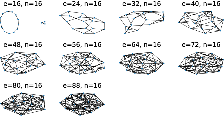
Figure B.2: Toy dataset for the investigation of effective target distributions. The dataset comprises 10 randomly generated regular graphs, each with 16 nodes and degrees ranging from 2 to 11.

Toy Dataset. For the toy dataset experiment, we conduct a sampling process where each model is allowed to generate 100 graphs. To determine the graph recall rate, we perform isomorphism testing utilizing the networkx[15] package. The training set’s visualization is provided in Fig. B.2.

Synthetic and Real-world Datasets. We consider the following synthetic and real-world graph datasets: (1) Ego-small: 200 small ego graphs from Citeseer dataset [51] with $|\mathcal{V}|\in[4,18]$, (2) Community-small: 100 random graphs generated by Erdős–Rényi model [13] consisting of two equal-sized communities whose $|\mathcal{V}|\in[12,20]$, (3) Grid: 100 random 2D grid graphs with $|\mathcal{V}|\in[100,400]$. (4) Protein: real-world DD protein dataset [11] that has 918 graphs with $|\mathcal{V}|\in[100,500]$. We follow the same setup in [34, 71] and apply random split to use 80% of the graphs for training and the rest 20% for testing. In evaluation, we generate the same number of graphs as the test set to compute the maximum mean discrepancy (MMD) of statistics like node degrees, clustering coefficients, and orbit counts. To compute MMD efficiently, we follow [34] and use the total variation distance kernel.

Molecule Datasets. We utilize the QM9 [50] and ZINC250k [22] as molecule datasets. To ensure a fair comparison, we use the same pre-processing and training/testing set splitting as in [24, 53, 38]. We generate 10,000 molecule graphs and compare the following key metrics: (1) validity w/o correction: the proportion of valid molecules without valency correction or edge resampling; (2) uniqueness: the proportion of unique and valid molecules; (3) Fréchet ChemNet Distance (FCD) [49]: activation difference using pretrained ChemNet; (4) neighborhood subgraph pairwise distance kernel (NSPDK) MMD [8]: graph kernel distance considering subgraph structures and node features. We do not report novelty (the proportion of valid molecules not seen in the training set) following [64, 63]. Specifically, the QM9 dataset provides a comprehensive collection of small molecules that meet specific predefined criteria. Generating molecules outside this set (a.k.a. novel graphs) does not necessarily indicate that the network has accurately captured the underlying data distribution.

Data Quantization. In this paper, we learn a continuous diffusion model for graph data. Following DDPM [18], we map the binary data into the range of [-1, 1] and add noise to the processed data during training. During sampling, we start with Gaussian noise. After the refinement, we map the results from [-1, 1] to [0, 1]. Since graphs are discrete data, we choose 0.5 as a threshold to quantize the continuous results. Similar approaches have been adopted in previous works [48, 24].

B.2 Network Architecture Details

	Hyperparameter	Ego-small	Community-small	Grid	DD Protein	QM9	ZINC250k
SwinGNN	Downsampling block layers	[4, 4, 6]	[4, 4, 6]	[1, 1, 3, 1]	[1, 1, 3, 1]	[1, 1, 3, 1]	[1, 1, 3, 1]
	Upsampling block layers	[4, 4, 6]	[4, 4, 6]	[1, 1, 3, 1]	[1, 1, 3, 1]	[1, 1, 3, 1]	[1, 1, 3, 1]
	Patch size	3	3	4	4	1	4
	Window size	24	24	6	8	4	5
	Token dimension	60	60	60	60	60	60
	Feedforward layer dimension	240	240	240	240	240	240
	Number of attention heads	[3, 6, 12, 24]	[3, 6, 12, 24]	[3, 6, 12, 24]	[3, 6, 12, 24]	[3, 6, 12, 24]	[3, 6, 12, 24]
	Number of trainable parameters	15.37M	15.37M	15.31M	15.31M	15.25M	15.25M
	Number of epochs	10000	10000	15000	50000	5000	5000
	EMA	0.9	0.99	0.99	0.9999	0.9999	0.9999
SwinGNN-L∗	Token dimension	96	96	96	96	96	96
	Feedforward layer dimension	384	384	384	384	384	384
	Number of trainable parameters	34.51M	35.91M	35.91M	35.91M	35.78M	35.78M
	Number of epochs	10000	10000	15000	50000	5000	5000
	EMA	0.99	0.95	0.95	0.9999	0.9999	0.9999
UNet-ADM∗	Channel multiplier	64	64	64	64	-	-
	Channels per resolution	[1, 2, 3, 4]	[1, 2, 3, 4]	[1, 2, 3, 4]	[1, 1, 1, 1, 2, 4, 6]	-	-
	Residule blocks per resolution	3	3	3	1	-	-
	Number of trainable parameters	30.86M	31.12M	29.50M	32.58M	-	-
	Number of epochs	5000	5000	15000	10000	-	-
	EMA	0.9999	0.99	0.999	0.9	-	-
Optimization	Optimizer	Adam	Adam	Adam	Adam	Adam	Adam
	Learning rate	$1.0\times 10^{-4}$	$1.0\times 10^{-4}$	$1.0\times 10^{-4}$	$1.0\times 10^{-4}$	$1.0\times 10^{-4}$	$1.0\times 10^{-4}$

Table B.1: Architecture details of the proposed SwinGNN and major baselines. ^∗The same hyper-parameters are employed for both SwinGNN and SwinGNN-L, barring specific exceptions outlined in the table. The UNet is adopted from [10] with their hyperparameters for the ImageNet-64 dataset.

Method	#params	BS=1	BS=2	BS=4	BS=8	BS=16	BS=32
GDSS	0.37M	3008M	4790M	8644M	15504M	OOM	OOM
DiGress	18.43M	16344M	19422M	22110M	OOM	OOM	OOM
EDP-GNN	0.09M	7624M	13050M	23848M	OOM	OOM	OOM
Unet	32.58M	6523M	10557M	18247M	OOM	OOM	OOM
SwinGNN	15.31M	2905M	3563M	5127M	8175M	14325M	OOM
SwinGNN-L	35.91M	4057M	5203M	7471M	12113M	21451M	OOM

Table B.2: Analysis of the GPU memory consumption during the training phase on a single NVIDIA RTX 3090 (24 GB) graphics card, where OOM stands for out-of-memory. Experiments are performed on the protein dataset that contains 918 graphs, each having a node count ranging from 100 to 500.

Our Models and Baselines. Tab. B.1 shows the network architecture details of our models and the UNet baselines on various datasets. Regarding the PPGN [41], we utilize the implementation in [43]. It takes an $n\times n$ noisy matrix as input and produces the denoised signal as output. To build non-permutation-equivariant version of PPGN, sinusoidal positional encoding [62] is applied at each layer. We use the same diffusion setup for PPGN-based networks and our SwinGNN, as specified in Tab. B.3. For a fair comparison, we utilize the publicly available code from the other baselines and run experiments using our dataset splits.

Network Expressivity. Both theoretical and empirical evidence have underscored the intrinsic connection between the WL test and function approximation capability for GNNs [40, 16, 6, 46, 42, 68]. The permutation equivariant PPGN layer, notable for its certified 3-WL test capacity, is deemed sufficiently expressive for experimental investigation. Further, it is crucial to note the considerable theoretical expressivity displayed by non-permutation-equivariant GNNs, particularly those with positional encoding [28, 14]. We argue that the GNNs employed in our studies theoretically have sufficient function approximation capacities, and therefore, the results of our research are not limited by the expressiveness of the network.

GPU Memory Usage. Our model’s efficiency in GPU memory usage during training, thanks to window self-attention and hierarchical graph representations learning, allows for faster training compared to models with similar parameter counts. In Tab. B.2, we compare the training memory costs for various models with different batch sizes using the real-world protein dataset.

B.3 Node and Edge Attribute Encoding

Molecules possess various edge types, ranging from no bond to single, double, and triple bonds. Also, they encompass diverse node types like C, N, O, F, and others. We employ three methods to encode the diverse node and edge attributes: 1) scalar representation, 2) binary bits, and 3) one-hot encoding.

Scalar Encoding. We divide the interval [-1, 1] into several equal-sized sub-intervals (except for the intervals near the boundaries), with each sub-interval representing a specific type. We quantize the node or edge attributes in the samples based on the sub-interval to which it belongs as in [24].

Binary-bit Encoding. Following [5], we encode attribute integers using multi-channel binary bits. For better training dynamics, we remap the bits from 0/1 to -1/1 representation. During sampling, we perform quantization for the continuous channel-wise bit samples and convert them back to integers.

One-hot Encoding. We adopt a similar process as the binary-bit encoding, up until the integer-vector conversion. We use argmax to quantize the samples and convert them to integers.

Network Modifications. We concatenate the features of the source and target node of an edge to the original edge feature, creating multi-channel edge features as the augmented input. At the final readout layer, we use two MLPs to convert the shared edge features for edge and node denoising.

B.4 Diffusion Process Hyperparameters

$c_{s}(\sigma)=\frac{\sigma_{d}^{2}}{\sigma_{d}^{2}+\sigma^{2}}$	$c_{o}(\sigma)=\frac{\sigma\sigma_{d}}{\sqrt{\sigma_{d}^{2}+\sigma^{2}}}$
$c_{i}(\sigma)=\frac{1}{\sqrt{\sigma_{d}^{2}+\sigma^{2}}}$	$c_{n}(\sigma)=\frac{1}{4}\ln(\sigma)$
$\sigma_{d}=0.5,\ln(\sigma)\sim\mathcal{N}(P_{\text{mean}},P_{\text{std}}^{2}),P_{\text{mean}}=-P_{\text{std}}=-1.2$
$\sigma_{\text{min}}=0.002,\sigma_{\text{max}}=80,\rho=7$
$S_{\text{tmin}}=0.05,S_{\text{tmax}}=50,S_{\text{noise}}=1.003,S_{\text{churn}}=40,N=256$
$t_{i}=({\sigma_{\text{max}}}^{\frac{1}{\rho}}+\frac{i}{N-1}({\sigma_{\text{min}}}^{\frac{1}{\rho}}-{\sigma_{\text{max}}}^{\frac{1}{\rho}}))^{\rho}$
$\gamma_{i}=\boldsymbol{1}_{S_{\text{tmin}}\leq t_{i}\leq S_{\text{tmax}}}\cdot\min(\frac{S_{\text{churn}}}{N},\sqrt{2}-1)$

Table B.3: Training and sampling hyperparameters in the diffusion process.

The hyperparameters of the diffusion model training and sampling steps are summarized in Tab. B.3. For our SwinGNN model, we maintain a consistent setup throughout the paper, unless stated otherwise. This setup is used for various experiments, including the ablation studies where we compare against the vanilla DDPM [18] and the toy dataset experiments.

The pivotal role of refining both the training and sampling phases in diffusion models to bolster performance has been emphasized in prior literature [56, 47, 27]. Such findings, validated across a broad spectrum of fields beyond image generation [52, 70], inspired our adoption of the most recent diffusion model framework. For a detailed discussion on the principles of hyperparameter fine-tuning, readers are encouraged to refer to the previously mentioned studies.

B.5 Comparing against the SwinTransformer Baseline

	Ego-Small			Community-Small			Grid			Protein
Methods	Deg. $\downarrow$	Clus. $\downarrow$	Orbit. $\downarrow$	Deg. $\downarrow$	Clus. $\downarrow$	Orbit. $\downarrow$	Deg. $\downarrow$	Clus. $\downarrow$	Orbit. $\downarrow$	Deg. $\downarrow$	Clus. $\downarrow$	Orbit. $\downarrow$
SwinGNN	3.61e-4	2.12e-2	3.58e-3	2.98e-3	5.11e-2	4.33e-3	1.91e-7	0.00	6.88e-6	1.88e-3	1.55e-2	2.54e-3
SwinGNN-L	5.72e-3	3.20e-2	5.35e-3	1.42e-3	4.52e-2	6.30e-3	2.09e-6	0.00	9.70e-7	1.19e-3	1.57e-2	8.60e-4
SwinTF	8.50e-3	4.42e-2	8.00e-3	2.70e-3	7.11e-2	1.30e-3	2.50e-3	8.78e-5	1.25e-2	4.99e-2	1.32e-1	1.56e-1

Table B.4: Comparing our SwinGNN against the vanilla visual SwinTransformer [37].

To further demonstrate the effectiveness of our proposed network in handling adjacency matrices for denoising purposes, we include an additional comparison with SwinTransformer [37]. SwinTransformer is a general-purpose backbone network commonly used in visual tasks such as semantic segmentation, which also involves dense predictions similar to our denoising task.

In our experiments, we modify the SwinTF + UperNet [67] method and adapt it to output denoising signals. Specifically, we conduct experiments on the various graphs datasets, and the results are presented in Tab. B.4. The results clearly demonstrate the superior performance of our proposed SwinGNN model compared to simply adapting the visual SwinTransformer for graph generation.

B.6 Additional Qualitative Results

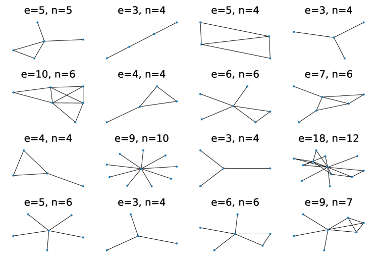
Figure B.3: Visualization of sample graphs generated by our model on the ego-small dataset.

Figure B.4: Visualization of sample graphs generated by our model on the community-small dataset.

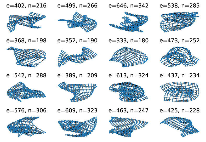
Figure B.5: Visualization of sample graphs generated by our model on the grid dataset.

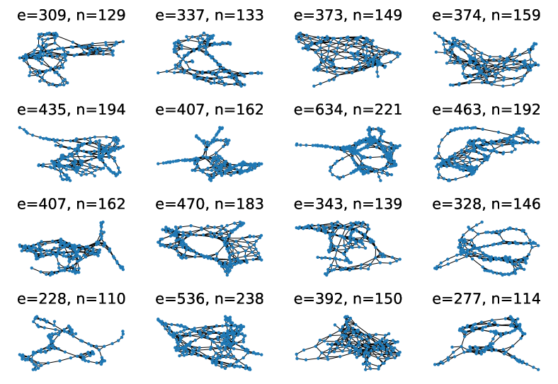
Figure B.6: Visualization of sample graphs generated by our model on the DD protein dataset.

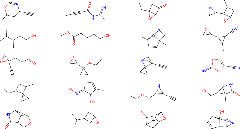
Figure B.7: Visualization of sample graphs generated by our model on the QM9 molecule dataset.

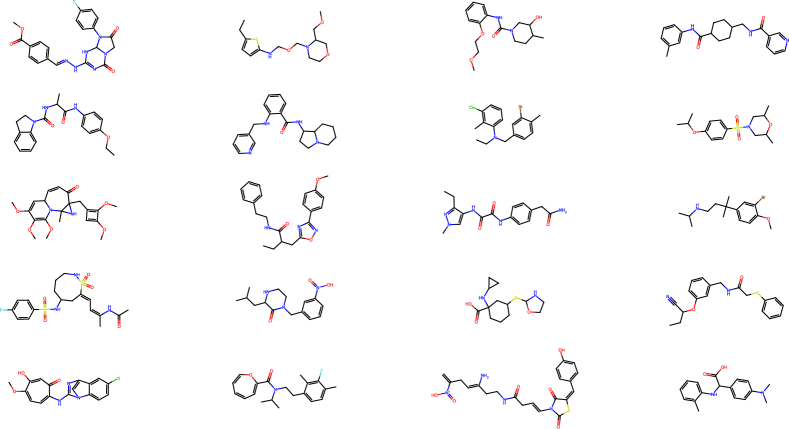
Figure B.8: Visualization of sample graphs generated by our model on the ZINC250k molecule dataset.

References

- [1] Réka Albert and Albert-László Barabási. Statistical mechanics of complex networks. Reviews of modern physics, 74(1):47, 2002.
- [2] Hassan Ashtiani, Shai Ben-David, Nicholas J. A. Harvey, Christopher Liaw, Abbas Mehrabian, and Yaniv Plan. Near-optimal sample complexity bounds for robust learning of gaussian mixtures via compression schemes. J. ACM, 67(6), oct 2020.
- [3] Jacob Austin, Daniel D. Johnson, Jonathan Ho, Daniel Tarlow, and Rianne van den Berg. Structured denoising diffusion models in discrete state-spaces. In Advances in Neural Information Processing Systems, 2021.
- [4] Marc Brockschmidt, Miltiadis Allamanis, Alexander L. Gaunt, and Oleksandr Polozov. Generative code modeling with graphs. In International Conference on Learning Representations, 2019.
- [5] Ting Chen, Ruixiang ZHANG, and Geoffrey Hinton. Analog bits: Generating discrete data using diffusion models with self-conditioning. In The Eleventh International Conference on Learning Representations, 2023.
- [6] Zhengdao Chen, Soledad Villar, Lei Chen, and Joan Bruna. On the equivalence between graph isomorphism testing and function approximation with gnns. In Advances in Neural Information Processing Systems, volume 32. Curran Associates, Inc., 2019.
- [7] Hang Chu, Daiqing Li, David Acuna, Amlan Kar, Maria Shugrina, Xinkai Wei, Ming-Yu Liu, Antonio Torralba, and Sanja Fidler. Neural turtle graphics for modeling city road layouts. In Proceedings of the IEEE/CVF International Conference on Computer Vision (ICCV), October 2019.
- [8] Fabrizio Costa and Kurt De Grave. Fast neighborhood subgraph pairwise distance kernel. In Proceedings of the 27th International Conference on International Conference on Machine Learning, ICML’10, page 255–262, Madison, WI, USA, 2010. Omnipress.
- [9] Nicola De Cao and Thomas Kipf. MolGAN: An implicit generative model for small molecular graphs. ICML 2018 workshop on Theoretical Foundations and Applications of Deep Generative Models, 2018.
- [10] Prafulla Dhariwal and Alexander Nichol. Diffusion models beat gans on image synthesis. In Advances in Neural Information Processing Systems, volume 34, pages 8780–8794. Curran Associates, Inc., 2021.
- [11] Paul D. Dobson and Andrew J. Doig. Distinguishing enzyme structures from non-enzymes without alignments. Journal of Molecular Biology, 330(4):771–783, 2003.
- [12] Bradley Efron. Tweedie’s formula and selection bias. Journal of the American Statistical Association, 106(496):1602–1614, 2011. PMID: 22505788.
- [13] P. Erdös and A. Rényi. On random graphs i. Publicationes Mathematicae Debrecen, 6:290, 1959.
- [14] Mohammad Fereydounian, Hamed Hassani, and Amin Karbasi. What functions can graph neural networks generate? arXiv preprint arXiv:2202.08833, 2022.
- [15] Aric Hagberg, Pieter Swart, and Daniel S Chult. Exploring network structure, dynamics, and function using networkx. Technical report, Los Alamos National Lab.(LANL), Los Alamos, NM (United States), 2008.
- [16] William L. Hamilton. Graph representation learning. Synthesis Lectures on Artificial Intelligence and Machine Learning, 14(3):1–159, 2020.
- [17] Jonathan Ho, William Chan, Chitwan Saharia, Jay Whang, Ruiqi Gao, Alexey Gritsenko, Diederik P Kingma, Ben Poole, Mohammad Norouzi, David J Fleet, et al. Imagen video: High definition video generation with diffusion models. arXiv preprint arXiv:2210.02303, 2022.
- [18] Jonathan Ho, Ajay Jain, and Pieter Abbeel. Denoising diffusion probabilistic models. In Advances in Neural Information Processing Systems, volume 33, pages 6840–6851. Curran Associates, Inc., 2020.
- [19] Emiel Hoogeboom, Didrik Nielsen, Priyank Jaini, Patrick Forré, and Max Welling. Argmax flows and multinomial diffusion: Learning categorical distributions. In Advances in Neural Information Processing Systems, volume 34, pages 12454–12465. Curran Associates, Inc., 2021.
- [20] Emiel Hoogeboom, Víctor Garcia Satorras, Clément Vignac, and Max Welling. Equivariant diffusion for molecule generation in 3D. In Proceedings of the 39th International Conference on Machine Learning, volume 162 of Proceedings of Machine Learning Research, pages 8867–8887. PMLR, 17–23 Jul 2022.
- [21] Jonathan H Huggins, Trevor Campbell, Mikołaj Kasprzak, and Tamara Broderick. Practical bounds on the error of bayesian posterior approximations: A nonasymptotic approach. arXiv preprint arXiv:1809.09505, 2018.
- [22] John J. Irwin, Teague Sterling, Michael M. Mysinger, Erin S. Bolstad, and Ryan G. Coleman. Zinc: A free tool to discover chemistry for biology. Journal of Chemical Information and Modeling, 52(7):1757–1768, 2012. PMID: 22587354.
- [23] Wengong Jin, Regina Barzilay, and Tommi Jaakkola. Junction tree variational autoencoder for molecular graph generation. In Proceedings of the 35th International Conference on Machine Learning, volume 80 of Proceedings of Machine Learning Research, pages 2323–2332. PMLR, 10–15 Jul 2018.
- [24] Jaehyeong Jo, Seul Lee, and Sung Ju Hwang. Score-based generative modeling of graphs via the system of stochastic differential equations. In Proceedings of the 39th International Conference on Machine Learning, volume 162 of Proceedings of Machine Learning Research, pages 10362–10383. PMLR, 17–23 Jul 2022.
- [25] Daniel D. Johnson, Jacob Austin, Rianne van den Berg, and Daniel Tarlow. Beyond in-place corruption: Insertion and deletion in denoising probabilistic models. In ICML Workshop on Invertible Neural Networks, Normalizing Flows, and Explicit Likelihood Models, 2021.
- [26] Oliver Johnson and Andrew Barron. Fisher information inequalities and the central limit theorem. Probability Theory and Related Fields, 129(3):391–409, Jul 2004.
- [27] Tero Karras, Miika Aittala, Timo Aila, and Samuli Laine. Elucidating the design space of diffusion-based generative models. In Advances in Neural Information Processing Systems, 2022.
- [28] Nicolas Keriven and Samuel Vaiter. What functions can graph neural networks compute on random graphs? the role of positional encoding. arXiv preprint arXiv:2305.14814, 2023.
- [29] Thomas N Kipf and Max Welling. Variational graph auto-encoders. NIPS Workshop on Bayesian Deep Learning, 2016.
- [30] Igor Krawczuk, Pedro Abranches, Andreas Loukas, and Volkan Cevher. Cg-gan: A geometric graph generative adversarial network, 2021.
- [31] Christophe Ley and Yvik Swan. Stein’s density approach and information inequalities. Electronic Communications in Probability, 18(none):1 – 14, 2013.
- [32] Muchen Li, Jeffrey Yunfan Liu, Leonid Sigal, and Renjie Liao. Graphpnas: Learning distribution of good neural architectures via deep graph generative models. arXiv preprint arXiv:2211.15155, 2022.
- [33] Renjie Liao. Graph neural networks: graph generation. Graph Neural Networks: Foundations, Frontiers, and Applications, pages 225–250, 2022.
- [34] Renjie Liao, Yujia Li, Yang Song, Shenlong Wang, Charlie Nash, William L. Hamilton, David Duvenaud, Raquel Urtasun, and Richard Zemel. Efficient graph generation with graph recurrent attention networks. In NeurIPS, 2019.
- [35] Phillip Lippe and Efstratios Gavves. Categorical normalizing flows via continuous transformations. In International Conference on Learning Representations, 2021.
- [36] Jenny Liu, Aviral Kumar, Jimmy Ba, Jamie Kiros, and Kevin Swersky. Graph normalizing flows. In Advances in Neural Information Processing Systems, volume 32. Curran Associates, Inc., 2019.
- [37] Ze Liu, Yutong Lin, Yue Cao, Han Hu, Yixuan Wei, Zheng Zhang, Stephen Lin, and Baining Guo. Swin transformer: Hierarchical vision transformer using shifted windows. In Proceedings of the IEEE/CVF International Conference on Computer Vision (ICCV), 2021.
- [38] Youzhi Luo, Keqiang Yan, and Shuiwang Ji. Graphdf: A discrete flow model for molecular graph generation. In Proceedings of the 38th International Conference on Machine Learning, volume 139 of Proceedings of Machine Learning Research, pages 7192–7203. PMLR, 18–24 Jul 2021.
- [39] Kaushalya Madhawa, Katushiko Ishiguro, Kosuke Nakago, and Motoki Abe. Graphnvp: An invertible flow model for generating molecular graphs. arXiv preprint arXiv:1905.11600, 2019.
- [40] Sadegh Mahdavi, Kevin Swersky, Thomas Kipf, Milad Hashemi, Christos Thrampoulidis, and Renjie Liao. Towards better out-of-distribution generalization of neural algorithmic reasoning tasks. Transactions on Machine Learning Research, 2023.
- [41] Haggai Maron, Heli Ben-Hamu, Hadar Serviansky, and Yaron Lipman. Provably powerful graph networks. In Advances in Neural Information Processing Systems, volume 32. Curran Associates, Inc., 2019.
- [42] Haggai Maron, Heli Ben-Hamu, Nadav Shamir, and Yaron Lipman. Invariant and equivariant graph networks. In International Conference on Learning Representations, 2019.
- [43] Karolis Martinkus, Andreas Loukas, Nathanaël Perraudin, and Roger Wattenhofer. SPECTRE: Spectral conditioning helps to overcome the expressivity limits of one-shot graph generators. In Proceedings of the 39th International Conference on Machine Learning, volume 162 of Proceedings of Machine Learning Research, pages 15159–15179. PMLR, 17–23 Jul 2022.
- [44] Rocío Mercado, Tobias Rastemo, Edvard Lindelöf, Günter Klambauer, Ola Engkvist, Hongming Chen, and Esben Jannik Bjerrum. Graph networks for molecular design. Machine Learning: Science and Technology, 2(2):025023, mar 2021.
- [45] Christopher Morris, Yaron Lipman, Haggai Maron, Bastian Rieck, Nils M Kriege, Martin Grohe, Matthias Fey, and Karsten Borgwardt. Weisfeiler and leman go machine learning: The story so far. arXiv preprint arXiv:2112.09992, 2021.
- [46] Christopher Morris, Martin Ritzert, Matthias Fey, William L. Hamilton, Jan Eric Lenssen, Gaurav Rattan, and Martin Grohe. Weisfeiler and leman go neural: Higher-order graph neural networks. Proceedings of the AAAI Conference on Artificial Intelligence, 33(01):4602–4609, Jul. 2019.
- [47] Alexander Quinn Nichol and Prafulla Dhariwal. Improved denoising diffusion probabilistic models. In Proceedings of the 38th International Conference on Machine Learning, volume 139 of Proceedings of Machine Learning Research, pages 8162–8171. PMLR, 18–24 Jul 2021.
- [48] Chenhao Niu, Yang Song, Jiaming Song, Shengjia Zhao, Aditya Grover, and Stefano Ermon. Permutation invariant graph generation via score-based generative modeling. In Proceedings of the Twenty Third International Conference on Artificial Intelligence and Statistics, volume 108 of Proceedings of Machine Learning Research, pages 4474–4484. PMLR, 26–28 Aug 2020.
- [49] Kristina Preuer, Philipp Renz, Thomas Unterthiner, Sepp Hochreiter, and Günter Klambauer. Fréchet chemnet distance: A metric for generative models for molecules in drug discovery. Journal of Chemical Information and Modeling, 58(9):1736–1741, 2018. PMID: 30118593.
- [50] Raghunathan Ramakrishnan, Pavlo O. Dral, Matthias Rupp, and O. Anatole von Lilienfeld. Quantum chemistry structures and properties of 134 kilo molecules. Scientific Data, 1(1):140022, Aug 2014.
- [51] Prithviraj Sen, Galileo Namata, Mustafa Bilgic, Lise Getoor, Brian Galligher, and Tina Eliassi-Rad. Collective classification in network data. AI Magazine, 29(3):93, Sep. 2008.
- [52] Wenkang Shan, Zhenhua Liu, Xinfeng Zhang, Zhao Wang, Kai Han, Shanshe Wang, Siwei Ma, and Wen Gao. Diffusion-based 3d human pose estimation with multi-hypothesis aggregation. arXiv preprint arXiv:2303.11579, 2023.
- [53] Chence Shi*, Minkai Xu*, Zhaocheng Zhu, Weinan Zhang, Ming Zhang, and Jian Tang. Graphaf: a flow-based autoregressive model for molecular graph generation. In International Conference on Learning Representations, 2020.
- [54] Martin Simonovsky and Nikos Komodakis. Graphvae: Towards generation of small graphs using variational autoencoders. In Artificial Neural Networks and Machine Learning–ICANN 2018: 27th International Conference on Artificial Neural Networks, Rhodes, Greece, October 4-7, 2018, Proceedings, Part I 27, pages 412–422. Springer, 2018.
- [55] Jascha Sohl-Dickstein, Eric Weiss, Niru Maheswaranathan, and Surya Ganguli. Deep unsupervised learning using nonequilibrium thermodynamics. In Proceedings of the 32nd International Conference on Machine Learning, volume 37 of Proceedings of Machine Learning Research, pages 2256–2265, Lille, France, 07–09 Jul 2015. PMLR.
- [56] Jiaming Song, Chenlin Meng, and Stefano Ermon. Denoising diffusion implicit models. In International Conference on Learning Representations, 2021.
- [57] Yang Song and Stefano Ermon. Improved techniques for training score-based generative models. In Advances in Neural Information Processing Systems, volume 33, pages 12438–12448. Curran Associates, Inc., 2020.
- [58] Yang Song, Jascha Sohl-Dickstein, Diederik P Kingma, Abhishek Kumar, Stefano Ermon, and Ben Poole. Score-based generative modeling through stochastic differential equations. In International Conference on Learning Representations, 2021.
- [59] Mohammed Suhail, Abhay Mittal, Behjat Siddiquie, Chris Broaddus, Jayan Eledath, Gerard Medioni, and Leonid Sigal. Energy-based learning for scene graph generation. In Proceedings of the IEEE/CVF Conference on Computer Vision and Pattern Recognition (CVPR), pages 13936–13945, June 2021.
- [60] Ananda Theertha Suresh, Alon Orlitsky, Jayadev Acharya, and Ashkan Jafarpour. Near-optimal-sample estimators for spherical gaussian mixtures. In Advances in Neural Information Processing Systems, volume 27. Curran Associates, Inc., 2014.
- [61] Endre Süli and David F. Mayers. An Introduction to Numerical Analysis. Cambridge University Press, 2003.
- [62] Ashish Vaswani, Noam Shazeer, Niki Parmar, Jakob Uszkoreit, Llion Jones, Aidan N Gomez, Łukasz Kaiser, and Illia Polosukhin. Attention is all you need. Advances in neural information processing systems, 30, 2017.
- [63] Clement Vignac and Pascal Frossard. Top-n: Equivariant set and graph generation without exchangeability. In International Conference on Learning Representations, 2022.
- [64] Clement Vignac, Igor Krawczuk, Antoine Siraudin, Bohan Wang, Volkan Cevher, and Pascal Frossard. Digress: Discrete denoising diffusion for graph generation. In The Eleventh International Conference on Learning Representations, 2023.
- [65] Pascal Vincent. A Connection Between Score Matching and Denoising Autoencoders. Neural Computation, 23(7):1661–1674, 07 2011.
- [66] Duncan J. Watts and Steven H. Strogatz. Collective dynamics of ‘small-world’ networks. Nature, 393(6684):440–442, Jun 1998.
- [67] Tete Xiao, Yingcheng Liu, Bolei Zhou, Yuning Jiang, and Jian Sun. Unified perceptual parsing for scene understanding. In Proceedings of the European conference on computer vision (ECCV), pages 418–434, 2018.
- [68] Keyulu Xu, Weihua Hu, Jure Leskovec, and Stefanie Jegelka. How powerful are graph neural networks? In International Conference on Learning Representations, 2019.
- [69] Minkai Xu, Lantao Yu, Yang Song, Chence Shi, Stefano Ermon, and Jian Tang. Geodiff: A geometric diffusion model for molecular conformation generation. In International Conference on Learning Representations, 2022.
- [70] Ling Yang, Zhilong Zhang, Yang Song, Shenda Hong, Runsheng Xu, Yue Zhao, Yingxia Shao, Wentao Zhang, Bin Cui, and Ming-Hsuan Yang. Diffusion models: A comprehensive survey of methods and applications. arXiv preprint arXiv:2209.00796, 2022.
- [71] Jiaxuan You, Rex Ying, Xiang Ren, William Hamilton, and Jure Leskovec. GraphRNN: Generating realistic graphs with deep auto-regressive models. In Proceedings of the 35th International Conference on Machine Learning, volume 80 of Proceedings of Machine Learning Research, pages 5708–5717. PMLR, 10–15 Jul 2018.
- [72] Kiarash Zahirnia, Oliver Schulte, Parmis Naddaf, and Ke Li. Micro and macro level graph modeling for graph variational auto-encoders. In Advances in Neural Information Processing Systems, 2022.