Magnetic field information in the near-ultraviolet
Fe II lines of the CLASP2 space experiment

Abstract

We investigate theoretically the circular polarization signals induced by the Zeeman effect in the Fe II lines of the $279.3$ - $280.7$ nm spectral range of the CLASP2 space experiment and their suitability to infer solar magnetic fields. To this end, we use a comprehensive Fe II atomic model to solve the problem of the generation and transfer of polarized radiation in semi-empirical models of the solar atmosphere, comparing the region of formation of the Fe II spectral lines with those of the Mg II h and k and the Mn I resonance lines. These are present in the same near ultraviolet (near-UV) spectral region and allowed the mapping of the longitudinal component of the magnetic field ($B_{\rm L}$) through several layers of the solar chromosphere in an active region plage. We compare our synthetic intensity profiles with observations from the IRIS and CLASP2 missions, proving the suitability of our model atom to characterize these Fe II spectral lines. The CLASP2 observations show two Fe II spectral lines at 279.79 and 280.66 nm with significant circular polarization signals. We demonstrate the suitability of the Weak-Field Approximation (WFA) applied to the Stokes $I$ and $V$ profiles of these Fe II lines to infer $B_{\rm L}$ in the plage atmosphere. We conclude that the near-UV spectral region of CLASP2 allows to determine $B_{\rm L}$ from the upper photosphere to the top of the chromosphere of active region plages.

1 Introduction

Understanding the structure and evolution of the magnetic field throughout the solar atmosphere is key to understanding the transfer of energy from the bottom of the photosphere to the chromosphere and to the million-degree corona. It is thus clear that observations and diagnostic tools allowing for a reliable and simultaneous inference of the magnetic field in different layers of the solar atmosphere, from the lower photosphere to the top of the chromosphere, just below the transition region to the corona, are necessary to improve our understanding of the physical processes taking place in the atmosphere of our closest star (e.g., Trujillo Bueno & del Pino Alemán, 2022).

Spectral lines encode information about the physical conditions of the plasma in their region of formation in the solar atmosphere. Many of the lines that form in the outer layers of the solar chromosphere are located in the UV region of the spectrum, which gives this spectral region significant potential for magnetic-field diagnostics across the solar atmosphere. For a recent review on the physics and diagnostic potential of UV spectropolarimetry, see Trujillo Bueno et al. (2017). In particular, two of the strongest and brightest spectral lines in the near-UV spectrum, the Mg II h and k resonant doublet, are located at 280.35 and 279.64 nm, respectively. The line center of these spectral lines originate just below the transition region, while their wings form in deeper layers between the lower and middle chromosphere (e.g., Leenaarts et al., 2013). Consequently, these spectral lines are among the most important for the study of the solar chromosphere.

Due to the significant opacity of the Earth’s atmosphere at UV wavelengths, these spectral lines can only be observed from space. The first spectropolarimetric data on the Mg II h and k lines were obtained by the Ultraviolet Spectrometer and Polarimeter (UVSP, Calvert et al., 1979; Woodgate et al., 1980) onboard the Solar Maximum Mission (SMM, Bohlin et al., 1980), which indicated the existence of significant scattering polarization signals in the far wings of these lines (Henze & Stenflo, 1987; Manso Sainz et al., 2019). Since 2013, their intensity spectrum has been systematically observed with the Interface Region Imaging Spectrograph mission (IRIS, De Pontieu et al., 2014), whose results have improved our knowledge about the thermal and dynamical structure of the upper layers of the solar chromosphere (see the review by De Pontieu et al., 2021).

Motivated by several theoretical studies on the polarization of the Mg II h and k lines around 280 nm (Belluzzi & Trujillo Bueno 2012; del Pino Alemán et al. 2016; Alsina Ballester et al. 2016, and del Pino Alemán et al. 2020), the Chromospheric LAyer SpectroPolarimeter (CLASP2, Song et al., 2022) suborbital mission was launched on April 11 2019, achieving unprecedented observations of the four Stokes parameters of this near-UV spectral region in an active region plage close to the solar disk center and in a quiet Sun region near the limb. The analysis of the quiet Sun spectral profiles confirmed the theoretical predictions on the scattering polarization signals (Rachmeler et al., 2022; Ishikawa et al., 2023). The application of the Weak-Field Approximation (WFA) to the circular polarization profiles observed in the plage region allowed for the mapping of the longitudinal component of the magnetic field ($B_{\rm L}$) across different layers of the solar chromosphere (Ishikawa et al., 2021), extended to the photosphere with simultaneous observations by Hinode/SOT-SP (Kosugi et al., 2007a). Later, the application of the Tenerife Inversion Code (TIC, Li et al., 2022) to the CLASP2 Stokes $I$ and $V$ profiles observed in the plage target allowed for the inference of a stratified model atmosphere, including its thermal, dynamic, and magnetic structure (Li et al., 2023).

Even though the analysis of the CLASP2 data has been limited, up to now, to the Mg II and Mn I lines, these observations show several other spectral lines with significant circular polarization signals. Among these lines, two Fe II spectral lines stand out: a relatively weak emission line at 279.79 nm and an absorption line at 280.66 nm, just at the red edge of the CLASP2 spectral window. Recent investigations have suggested that the Fe II lines located blueward of the CLASP2 spectral region are of complementary interest for diagnosing the magnetism of the solar chromosphere (see Judge et al., 2021, 2022). A quantitative study of the polarization signals and magnetic sensitivity of the Fe II spectral lines in the near-UV region of the solar spectrum has been recently published by Afonso Delgado et al. (2023a), but the Fe II lines located in the CLASP2 spectral region were not included in their work.

The pioneering results of the CLASP2 mission have proven the capabilities of the Mg II h and k spectral lines to study the magnetic field in the upper layers of the chromosphere. There has been a growing interest in the planning and development of space missions to perform full-Stokes observations of this spectral window, such as the Chromospheric Magnetism Explorer (CMEx, Gilbert, 2022). The analysis of the lines from species other than Mg II found in this spectral region is critical to take full advantage of the possibilities that future space missions bring to map the evolution of the magnetic field throughout the solar atmosphere.

In this paper we study the formation of the Fe II spectral lines in the CLASP2 spectral window, as well as their suitability to infer $B_{\rm L}$ and how they complement the magnetic field information that can be inferred from the Mg II and Mn I lines in the same spectral window (see Ishikawa et al., 2021). In Section 2 we describe the atomic models and our strategy to solve the radiation transfer (RT) problem. In Section 3 we analyze the emergent synthetic intensity profiles, studying the suitability of our model atom by comparing with observations at different lines of sight (LOS). In Section 4 we study the formation of the circular polarization profiles of the Fe II lines at 279.79 and 280.66 nm, and the suitability of the WFA to infer $B_{\rm L}$. We then apply the WFA to the CLASP2 data of these Fe II lines. Finally, in Section 5 we present our conclusions.

2 Formulation of the problem

Despite the significant number density of Fe II in the solar atmosphere, producing some of the strongest spectral lines in the near-UV solar spectrum (e.g., the resonant multiplet at 260 nm), the Fe II lines in the 279.3 - 280.7 nm spectral window are relatively weak (see Table 1 for their atomic data). In particular, both Fe II lines at 279.79 and 280.66 nm are intercombination lines. Because they form in the scattering wings of the Mg II h and k doublet, including the latter is necessary for an accurate modeling of these Fe II lines. Moreover, we also include an atomic model for the Mn I resonant triplet, also present in this spectral window.

As it is the case with most of the atomic lines located in the near-UV solar spectrum, the modeling of their intensity and polarization requires to account for strong departures from local thermodynamic equilibrium (LTE; e.g., Mihalas, 1978). In particular, one must jointly solve the statistical equilibrium equations (SEE) describing the populations and coherence between atomic sublevels, and the RT equations, describing the propagation of the electromagnetic radiation as it travels through the atmospheric plasma (e.g., Landi Degl’Innocenti & Landolfi, 2004). The Mg II h and k spectral lines show significant partial frequency redistribution (PRD) effects, and the modeling of their polarization requires accounting for $J$-state interference (Belluzzi & Trujillo Bueno, 2012, 2014; del Pino Alemán et al., 2016). Therefore, we account for $J$-state interference in our Mg II atom model (multi-term model atom; see §7.6 in Landi Degl’Innocenti & Landolfi, 2004), but we neglect it in the cases of the Fe II and Mn I atom models (multi-level model atom; see §7.2 in Landi Degl’Innocenti & Landolfi, 2004). We solve the RT problem accounting for all these physical ingredients with the HanleRT code (del Pino Alemán et al., 2016, 2020).

Our magnesium model atom comprises three Mg II terms, including the resonant doublet with PRD and the UV subordinate triplet with complete frequency redistribution (CRD), and the ground term of Mg III. This atomic model is the same used by del Pino Alemán et al. (2020) and Afonso Delgado et al. (2023b). Our atomic model for iron is the one described in Afonso Delgado et al. (2023a), to which we have added the atomic transition corresponding to the line at 279.79 nm, between the levels a⁴F_3/2 - z⁶D${}^{\circ}_{3/2}$ (the upper level is in the upper term of the resonant multiplet at 260 nm). The oscillator strength of this transition was taken from Kurucz & Bell (1995). Moreover, we determine the rate of inelastic collisions with free electrons and the photoionization cross-section by applying the approximations of van Regemorter (1962), Bely & van Regemorter (1970), and Allen (1963). We adjust the collisional rates through an ad-hoc factor in order to fit the line core intensity flux of the Fe II resonant transitions between 258.6 and 260.25 nm in the quiet Sun C model of Fontenla et al. (1993) to the observed flux of the solar analog $\alpha$ Cen A (see Afonso Delgado et al., 2023a, for further details).

An accurate modeling of the Mn I resonant doublet requires accounting for the hyperfine structure (HFS, see del Pino Alemán et al., 2022). The impact of the HFS is particularly relevant regarding the circular polarization profiles. However, it is not critical for estimating the region of formation of the lines. In this work we thus neglect the HFS, using an atomic model with four Mn I levels and the ground level of Mn II, with the resonant triplet in CRD.

Accounting for PRD and $J$-state interference in Mg II and, at the same time, for the large number of levels and transitions in the Fe II model atom, makes the simultaneous solution of the RT problem prohibitively expensive in terms of computing resources. Moreover, solving the non-LTE problem for both Fe II and Mg II affects the ionization balance of the latter (one of the reasons being the lack of Fe I as a source of background opacity in the far-UV). Therefore, we have opted for the following strategy:

1. Calculate jointly the population balance for Mg II and Mn I.

2. Calculate, independently, the population balance for Fe II.

3. Solve jointly the non-magnetic RT problem with the three atomic models by fixing the populations calculated in steps 1 and 2.

4. For the magnetic field problem, use a reduced model of Fe II with just five atomic levels (the upper and lower levels of the transitions at 279.79 and 280.66 nm, and the ground level of Fe III), still fixing the populations to those calculated in steps 1 and 2.

In this work we solve the RT problem in the 1D, plane-parallel, semi-empirical C and P atmospheric models described in Fontenla et al. (1993, hereafter FAL-C and FAL-P, respectively), representative of the quiet Sun and a plage region.

Table 1: Atomic data and effective Landé factor for Fe II atomic transitions in the spectral region of CLASP2.

$\lambda$ [nm]	Transition	Levels energy	Aul [s-1]	geff
279.471	a4G9/2 - z4I${}^{\circ}_{11/2}$	25 805 - 61 587	$1.3\cdot 10^{7}$	0.78a
279.787	a4F3/2 - z6D${}^{\circ}_{5/2}$	3 117 - 38 858	$1.9\cdot 10^{4}$	2.60b
280.012	b2H9/2 - y4F${}^{\circ}_{7/2}$	26 352 - 62 065	$1.5\cdot 10^{7}$	0.45b
280.485	a2F5/2 - x4D${}^{\circ}_{5/2}$	27 620 - 63 272	$1.6\cdot 10^{6}$	1.01b
280.661	a2F7/2 - x4D${}^{\circ}_{7/2}$	27 314 - 62 945	$3.2\cdot 10^{6}$	1.38b

^aLS coupling, accounting for the upper level coupling between ⁴H${}^{\circ}_{11/2}$ and ⁴G${}^{\circ}_{11/2}$

^bexperimental (Kramida et al., 2020)

3 Intensity Profiles

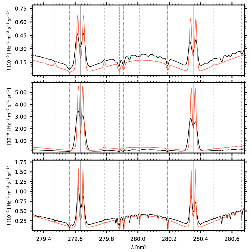
Figure 1: Emergent intensity profile for the spectral region observed by the CLASP2 mission for an LOS close to the solar limb ($\mu=0.1$; upper panel), for a pixel located in the active solar plage observed by CLASP2 ($\mu=0.7$, middle panel), and for an LOS at the solar disk center ($\mu=1$; lower panel). The red solid curves in upper and lower panels show our calculation in the FAL-C model atmosphere and in the middle panel it shows our calculation in the FAL-P model atmosphere. The black solid curve in the top (middle) panel is an average over 2 arcsec of the CLASP2 slit limb (plage) target observation. The black solid curve in the bottom panel is the average over all the field of view in a quiet Sun region observed by IRIS on October 4 2022. The vertical gray lines indicate the positions of the spectral lines: Mg II h and k (solid), Mg II subordinate lines (dashed), Mn I resonant triplet (dashed-dotted), and Fe II lines (dotted).

We compare, qualitatively, the synthetic intensity profiles with available observations (see Fig. 1). Within the CLASP2 spectral window we can find five Fe II spectral lines showing significant absorption or emission signals in both the theoretical and observed intensity profiles (indicated with gray-dotted lines in the figure). The upper panel of Fig. 1 shows the theoretical profile for an LOS with $\mu=\cos{\theta}=0.1$ (with $\theta$ the heliocentric angle of the observed point) together with the CLASP2 observation of a quiet Sun region close to the solar limb after averaging over 2 arcsec along the slit. The lower panel shows a comparison of the theoretical profiles for an LOS with $\mu=1.0$ together with the average of all the profiles contained in a whole map of an IRIS observation of the quiet Sun at the solar disk center from October 4 2022. Despite the limitations of using semi-empirical and static atmospheric models, the synthetic spectral lines show a qualitative behavior close to that of the observations. One exception to this is the Fe II line at 279.47 nm which seems to be not accurately represented by our atomic model. In the observations this spectral line is always in absorption while in our calculations it shows clear emission features both at disk-center and close to the limb.

There is a notable difference between synthetic and observed profiles in the Mg II h and k wings (see Fig.1). This disagreement is due to the different temperature in the formation region of the wings (upper photosphere) between the semi-empirical models and the actual atmospheric plasma. In the quiet-Sun (plage) observations, this temperature is lower (higher) than in the FAL-C (FAL-P) model. Note, however, that this difference in the quiet Sun observations is significantly diminished when comparing with the disk center observation from IRIS (bottom panel of Fig.1). In this case we average a larger number of profiles and, consequently, the semi-empirical “average” quiet Sun model FAL-C is much closer to the average of the quiet Sun observation.

The Fe II lines at 280.01 and 280.66 nm show significant absorption for an LOS at disk center and a relatively weaker absorption for an LOS toward the limb, for both theoretical and observed profiles. The Fe II lines at 279.79 and 280.48 nm show a relatively weak emission at disk center, which becomes more significant for LOS closer to the limb. We emphasize, in particular, that the model successfully reproduces the behavior for different LOS for the Fe II line at 279.79 nm, almost imperceptible for the disk center LOS and with a clear emission for an LOS close to the limb.

The CLASP2 observations in the plage region also show a significant emission feature in the Fe II line at 279.79 nm (see Ishikawa et al., 2021), despite the location of the plage being close to disk center (between $\mu=0.8$ and $0.6$). A spectral synthesis in the FAL-P model, representative of a solar plage, also shows a remarkable emission (see middle panel in Fig. 1).

These results support the suitability of the Fe II atomic model presented in Afonso Delgado et al. (2023a) for the present research.

4 Circular Polarization Profiles

In this section we study the formation of the circular polarization profiles of the Fe II lines in the CLASP2 spectral window. To this end, we impose an ad-hoc exponential stratification of the magnetic field (see the right panel of Fig. 2) in the FAL-C model atmosphere. None of the Fe II spectral lines mentioned in Sec. 3 show any linear polarization signals, either in the CLASP2 observations or in our numerical modeling. These lines show a quenching of the linear polarization in the Mg II h and k wings. This depolarization appears to be insensitive to artificial changes of the rate of the depolarizing collisions of the Fe II atomic model, indicating that the lines are just depolarizing the Mg II wings and do not show intrinsic polarization. Therefore, from now on we focus on the circular polarization profiles.

4.1 Theoretical Circular Polarization Profiles.

In the CLASP2 observations of an active region plage, only two of the Fe II spectral lines mentioned in Sec. 3 show clear circular polarization signals. These are the Fe II lines at 279.79 and 280.66 nm. The Fe II lines at 279.471 and 280.012 nm have relatively small effective Landé factors (0.78 and 0.45, respectively), and their circular polarization signals may be below the noise level as shown in Fig. 3. The Fe II at 280.485 nm is very weak for an LOS close to disk center (the plage region observed by CLASP2 is at $\mu\sim 0.8$), which can explain the absence of clear circular polarization signals. Therefore, in the following we focus on the Fe II lines at 279.79 and 280.66 nm.

To study in detail the circular polarization signals in these two lines, we solve the RT problem in the FAL-C model atmosphere for a disk-center LOS as described in Sec. 2, assuming a vertical magnetic field with strength decreasing exponentially with height, from 200 G in the bottom of the photosphere to 40 G just below the transition region (see the right panel of Fig. 2).

Under proper conditions, the WFA provides a fast method to estimate $B_{\rm L}$. For it to be applicable, the Doppler width of the line $\Delta\lambda_{D}=\frac{\lambda_{0}}{c}\sqrt{\frac{2kT}{m}+v_{\rm m}^{2}}$, (with $T$ and $v_{\rm m}$ the temperature and turbulent velocity, respectively, $c$ the speed of light, $k$ the Boltzmann constant, $m$ the mass of the atom, and $\lambda_{0}$ the line’s wavelength), must be much larger than the magnetic Zeeman splitting ($\Delta\lambda_{B}=4.6686\cdot 10^{-13}B\lambda_{0}^{2}$, with $B$ the magnetic field strength in gauss and $\lambda_{0}$ in angstroms); i.e.

$$g_{\rm eff}\frac{\Delta\lambda_{B}}{\Delta\lambda_{D}}\ll 1.$$ (1)

When this condition is met, and $B_{\rm L}$ is constant across the line formation region, the circular polarization profile is proportional to the wavelength derivative of the intensity (e.g., Landi Degl’Innocenti & Landolfi (2004))

$$V=-4.6686\cdot 10^{-13}g_{\rm eff}\lambda_{0}^{2}B_{L}\frac{\partial I}{\partial\lambda}.$$ (2)

The first and second columns of Fig. 2 show the circular polarization of the Mg II k and h lines (upper row), the Mn I lines at 279.91 and 280.19 nm (middle row), and the Fe II lines at 279.79 and 280.66 nm (bottom row). The colored background shows the logarithm of the normalized contribution function for Stokes $V$, which indicates the contribution of each region in the model atmosphere (see the height in the right axis in each panel) to the emergent circular polarization profiles. Red (blue) color indicates positive (negative) contributions to the circular polarization.

As shown in previous works, the contribution function indicates that the circular polarization in the inner lobes of the Mg II h and k lines form in the upper chromosphere, while the circular polarization in the outer lobes forms in a relatively extensive region in the middle chromosphere of the FAL-C model. The application of the WFA independently to each of these spectral regions allows us to fit the circular polarization profiles of all the selected spectral lines. We have excluded the outer lobes of the Mg II k line in this work because the blue outer lobe is blended with a Mn I line, impacting its circular polarization signal. The $B_{\rm L}$ values inferred with the WFA are found in the model atmosphere at those heights with the largest values of the contribution function (compare the contribution function in the first and second columns of Fig. 2 with the colored dots in the rightmost panel).

The region of formation of the circular polarization of the Mn I resonant lines is below that of the outer lobes of the Mg II h and k, thus between the lower and middle chromosphere in FAL-C.

Moreover, the WFA can be applied to the observations using the effective Landé factor calculated assuming LS coupling without HFS (del Pino Alemán et al., 2022). All the results shown here regarding the Mg II and Mn I lines in this spectral window agree with previous results (del Pino Alemán et al. 2020, 2022; Ishikawa et al. 2021).

Figure 2: Emergent fractional circular polarization profiles $V/I$ (first and second columns) for the Mg II k and h lines (first row), Mn I lines at 279.91 and 280.19 nm (second row), and Fe II lines at 279.787 and 280.661 nm (third row), for a disk center LOS, calculated in the FAL-C model with a vertical magnetic field with an exponential stratification (see rightmost panel). The colored background in the first two columns shows the logarithm of the normalized contribution function for the circular polarization (with the red and blue colors indicating positive and negative contributions, respectively). The colored curves in the first and second columns show the fit with the WFA. The outer lobes of the k line are excluded from the WFA fitting. The colored circles in the rightmost panel show the $B_{\rm L}$ value from the fit with the WFA of the circular polarization profile corresponding to the curve of the same color, placed at its intersection with the $B_{\rm L}$ stratification of the model. The colored solid lines help to quickly find the height and $B_{\rm L}$ values for each colored circle in the intersection between each line and the coordinate axes. The brown and magenta lines and circles overlap in the rightmost panel.

The Fe II line at 279.79 nm shows a circular polarization profile with four lobes, due to what seems to be a self-absorption feature in the center of the line (see the lower panel of Fig. 1). The inner lobes resulting from the numerical calculation cannot be observed with the CLASP2 spectral sampling ($\sim$0.01 nm), and thus the CLASP2 observations show a two-lobes circular polarization profile. The contribution function indicates that the circular polarization of this Fe II line forms mainly at heights between 0.3 and 0.5 Mm in the FAL-C model, which corresponds to the upper photosphere. The $B_{\rm L}$ inferred with the WFA corresponds to the actual value in the model at a height of 0.2 Mm, just below the formation region deduced from the contribution function.

The Fe II line at 280.66 nm, the one at the red edge of the CLASP2 spectral window, shows a more typical antisymmetric shape with two lobes, with signals larger than those of the Fe II line at 279.79 nm. From the contribution function, the region of formation of the circular polarization appears to be located at heights between 0.2 and 0.7 Mm in the upper photosphere of the FAL-C model. The $B_{\rm L}$ inferred with the WFA corresponds to the field expected at those heights.

As illustrated at the beginning of this section, the WFA can only be applied if Eq. (1) is satisfied. In Fig. 4 we show the stratification of the ratio $g_{\rm eff}\frac{\Delta\lambda_{B}}{\Delta\lambda_{D}}$ for the Fe II lines at 279.79 and 280.66 nm for different uniform magnetic fields, for both the FAL-C and FAL-P models. In typical applications to solar spectropolarimetry, the weak field condition of the WFA is often satisfied when the ratio in Eq. 1 is smaller than about 0.5. Consequently, for these lines that form around the temperature minimum ($\sim 0.5$ Mm, which would be the worst case scenario), the WFA would be suitable for magnetic fields up to about 500 G for the Fe II line at 279.79 nm and up to about 1000 G for the Fe II line at 280.66 nm.

Figure 3: Fractional circular polarization $V/I$ in a selected pixel in the CLASP2 plage observation (black dots, with error bars). The gray line shows the corresponding intensity profile (see right axis). The colored curves show the WFA fit for the seven spectral regions indicated in Fig. 2, in the same colors: the inner and outer lobes of the Mg II h line (red and light blue, respectively), the inner lobes of the Mg II k line (blue), the Mn I resonant lines (brown and magenta), and the Fe II lines at 279.79 and 280.66 nm (green and orange, respectively). The $B_{\rm L}$ inferred for each of them is indicated in the top-right inset.

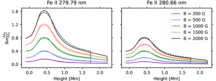
Figure 4: Stratification of the ratio $g_{\rm eff}\frac{\Delta\lambda_{B}}{\Delta\lambda_{D}}$ in the FAL-C (solid curves) and FAL-P (dashed curves) models, for a uniform magnetic field, for the Fe II lines at 279.79 nm (left panel) and at 280.66 nm (right panel). The colors of the curves indicate the magnetic field strength (see legend in the right panel).

In summary, the Fe II lines at 279.79 and 280.66 nm form in the upper photosphere, considerably deeper than the Mg II and Mn I in the same spectral range, and the WFA can be applied for a quick inference of $B_{\rm L}$ for longitudinal components of the magnetic field up to 500 G (for the 279.79 nm line) and up to 1000 G (for the 280.66 nm line).

4.2 Application to the CLASP2 data

The intensity and circular polarization profiles of the Mg II h and k lines and of the Mn I resonant lines observed by CLASP2 in a solar plage region have been analyzed in Ishikawa et al. (2021), mapping the longitudinal component of the magnetic field from the photosphere to the upper chromosphere. The $B_{\rm L}$ in the lower chromosphere was inferred by applying the WFA to the Mn I resonant lines. The $B_{\rm L}$ in the middle chromosphere was inferred by applying the WFA to the outer lobes of the Mg II h line. The $B_{\rm L}$ in the upper chromosphere was inferred by applying the WFA to the inner lobes of the Mg II h and k lines. The determination of the photospheric $B_{\rm L}$, however, resulted from a Milne-Eddington inversion of the Fe I lines at 630.15 and 630.25 nm, from data acquired in a simultaneous observation by the Hinode SOT-SP (Kosugi et al., 2007b). These lines form in the lower layers of the solar photosphere (Grec et al., 2010; Faurobert et al., 2012). In this section we extend the work of Ishikawa et al. (2021) by adding the inference of $B_{\rm L}$ by applying the WFA to the Fe II lines at 279.79 and 280.66 nm, as we did with the synthetic profiles in Sec. 4.1.

Figure 3 shows the fractional circular polarization in one pixel of the CLASP2 observation of a plage region. We apply the WFA to the same seven spectral regions indicated in Sec. 4.1. We get $B_{\rm L}$ between 179 and 193 G in the upper chromosphere (from the inner lobes of the Mg II h and k lines), 227 G in the middle chromosphere (from the outer lobes of the Mg II h line), and between 370 and 378 G in the lower chromosphere (from the Mn I lines). To this $B_{\rm L}$ stratification we can add 646 G in the upper photosphere (derived from the Fe II line at 280.66 nm). As expected, we obtain a $B_{\rm L}$ which increases with the depth of the region of formation of each spectral range.

In contrast, we find that the inferred $B_{\rm L}$ is 219 G when the WFA is applied to the Fe II at 279.79 nm. This is in apparent contradiction with the findings in Sec. 4.1, as this value is very close to the one obtained from the outer lobes of the Mg II h line, which forms in the middle chromosphere whereas, according to the numerical modeling of Sect.4.1, the Fe II 279.79 nm line should be the one that forms in the lowest part of the atmosphere, among the lines included in this work. This discrepancy can be understood by analyzing the formation of this spectral line in two semi-empirical models representative of the the quiet Sun (FAL-C) and a plage region (FAL-P).

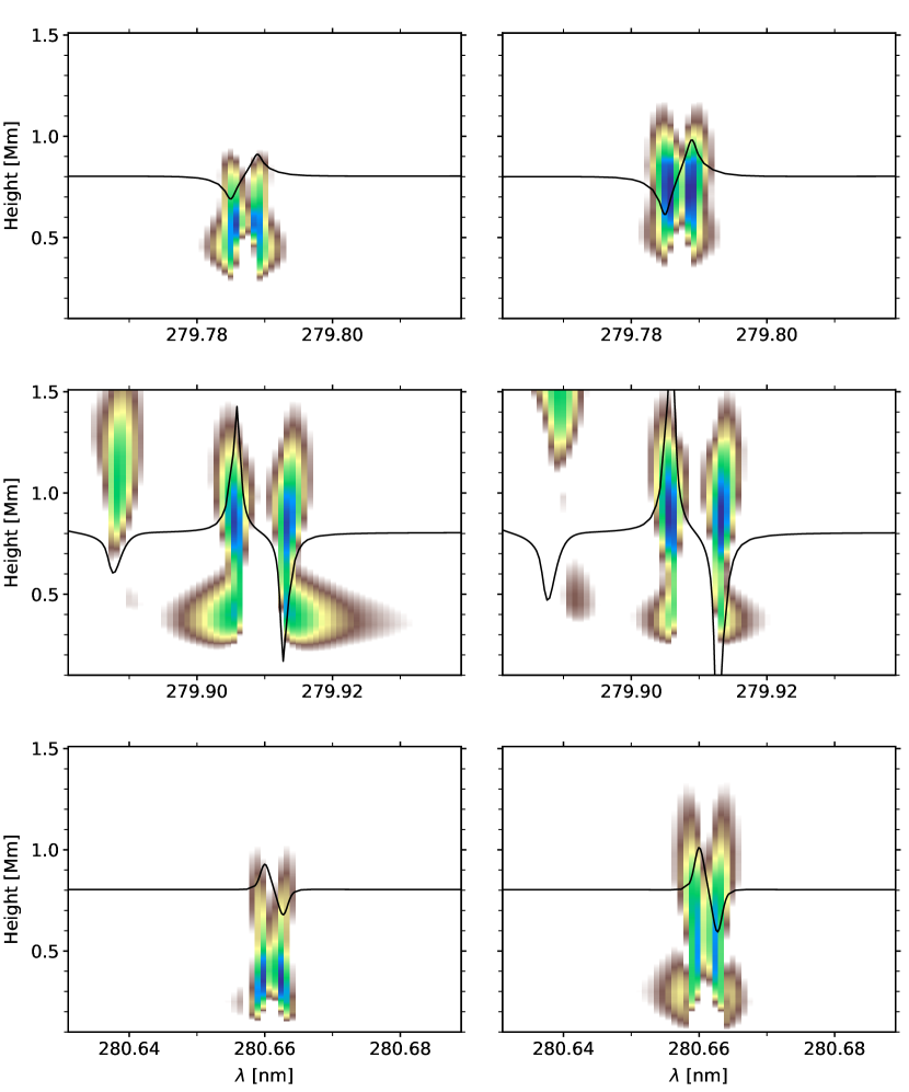
Figure 5: Fractional circular polarization $V/I$ calculated in the FAL-C (top row) and FAL-P (bottom row) semi-empirical model atmospheres. Each column shows the wavelength range around a spectral line: Fe II 279.79 nm (left), Mn I 279.91 nm (middle), and Fe II 280.66 nm (right). The colored background shows the absolute value of the logarithm of the normalized contribution function for the circular polarization, with the blue (brown) showing the regions with larger (lower) contribution.

In Fig. 5, we show the absolute value of the logarithm of the contribution function for the two Fe II (279.79 and 280.66 nm) and the Mn I (279.91 nm) lines calculated in the FAL-C and FAL-P model atmospheres. The blue regions correspond to the largest contribution to the circular polarization. In the quiet Sun model (top row of Fig. 5) the largest contribution for the two Fe II spectral lines is located at very similar heights, deeper in the atmosphere compared to the Mn I spectral line. However, in the plage region model (bottom row of Fig. 5) the largest contribution for the 279.79 nm line is higher in the atmosphere with respect to the other spectral lines. In this model this Fe II line forms at a height which is very similar to that of the Mn I line. Instead, the Fe II 280.66 nm line formation region is found always in deeper layers than the Mn I line.

In summary, while in quiet Sun conditions both Fe II lines form in relatively similar regions, in the plage region the formation of the Fe II line at 279.79 nm is shifted upwards relative to the other lines. This explains why, when applying the WFA approximation to the CLASP2 data in the plage region, we infer $B_{\rm L}$ values from the Fe II line at 279.79 nm that are smaller than those inferred from both the Fe II line at 280.66 nm and the Mn I lines.

With this more complete picture of the region of formation of the circular polarization of the lines in the CLASP2 spectral window we apply the WFA to the seven spectral regions specified in Fig. 2 in all pixels of the CLASP2 plage region observation. Fig. 6 shows the inferred $B_{\rm L}$ along the spectrograph slit. We include in the figure the $B_{\rm L}$ WFA inference from the Mg II h and k lines (top and middle chromosphere, red and black, respectively) and the Mn I lines (lower chromosphere, blue dots), which were presented in Ishikawa et al. (2021), as well as the result of their inversion of the Hinode data (light green curve). The $B_{\rm L}$ values we infer from the Mg II and Mn I spectral lines are very similar to those shown in Ishikawa et al. (2021).

The important new result in Fig. 6 is the $B_{\rm L}$ resulting from the application of the WFA to the Fe II lines at 279.79 and 280.66 nm (dark green and orange dots). The $B_{\rm L}$ inferred from the Fe II line at 280.66 nm is larger than for the other lines in the CLASP2 spectral window, and relatively close to the Milne-Eddington inversion of the Hinode data. This is in agreement with the expected photospheric region of formation of this spectral line. The $B_{\rm L}$ inferred from the Fe II line at 279.79 nm is instead similar to the values inferred for the middle chromosphere inside the plage region (slit positions from -99 to $\sim$ -70 arcsec and from $\sim$ -50 to $\sim$25 arcsec). Instead, in the nearby quiet Sun the inferred $B_{\rm L}$ is similar to the inference from the Fe II line at 280.66 nm, which is fully consistent with the change in the region of formation shown in Fig. 5.

Figure 6: Inferred $B_{\rm L}$ along the CLASP2 spectrograph slit. The light-green curve corresponds to the lower photosphere, obtained from the Milne-Eddington inversion of the Hinode/SOT-SP observation. The colored circles correspond to the inference applying the WFA to the seven spectral regions shown in Fig. 2: red circles: upper chromosphere inferred from the inner lobes of the Mg II h and k lines; blue circles, middle chromosphere inferred from the outer lobes of the Mg II h line; black circles, bottom chromosphere inferred from the Mn I lines; orange circles, upper photosphere inferred from the Fe II line at 280.66 nm, and dark green circles, middle chromosphere (top photosphere) in the plage region (quiet Sun region) inferred from the Fe II line at 279.79 nm. The lower panel shows a zoom in the magnetic field axis.

5 Conclusions

We investigated theoretically the formation of the intensity and circular polarization profiles of the Fe II lines located in the CLASP2 spectral window, comparing their region of formation with those of the Mg II and Mn I lines in the same spectral window, which were considered in previous studies. To this end, we solved the RT problem in a semi-empirical model atmosphere representative of the quiet Sun, to which we added an ad-hoc stratification of the magnetic field. In particular, we studied the formation of those Fe II spectral lines and their suitability to infer $B_{\rm L}$ by applying the WFA. We demonstrated the validity of this approximation and apply it to the CLASP2 data, extending the mapping of the longitudinal component of the magnetic field in Ishikawa et al. (2021) to additional layers of the solar atmosphere, between the upper photosphere and the lower chromosphere.

We compared the intensity emerging from the FAL-C model atmosphere, with observations by IRIS and CLASP2, for two LOS, one at disk center and one close to the limb. With the exception of the 279.47 nm line, all the Fe II lines in this spectral region show good qualitative agreement between the numerical calculations and the observations. This indicates that the Fe II model atom presented in Afonso Delgado et al. (2023a), is suitable to model the Fe II lines in this spectral window. In particular, the model reproduces the peculiar behavior of the Fe II line at 279.79 nm, almost absent at disk center, but with a clear emission at the solar limb or in active regions such as plage regions. We note that there is a Fe II line at 369.94 nm, in the red wing of the Ca II H line, which shows the same behavior, with an absorption profile at disk center, but an emission profile closer to the limb (Cram et al., 1980; Watanabe & Steenbock, 1986). In a future investigation, we will study the formation of this spectral line, which can be observed with ground-based facilities such as the Daniel K. Inouye Solar Telescope (DKIST, Rimmele et al., 2020).

We have found that only two of these five Fe II lines (279.471, 279.787, 280.012, 280.485, and 280.661 nm) show circular polarization signals above the noise level in the CLASP2 observations. By solving the RT problem in the FAL-C model (Sec. 4.1), we showed that both lines form in the photosphere when the thermodynamical conditions of the observed target are similar to those of the quiet Sun. We showed that the WFA of these lines can be applied for $B_{\rm L}$ up to 500 G for the 279.79 nm line and up to 1000 G for the 280.66 nm line.

We also found that the exact region of formation of the Fe II line at 279.79 nm depends on the particular physical conditions of the atmospheric plasma. While in the typical conditions of the quiet Sun this line forms in the photosphere, like the Fe II line at 280.66 nm, for the typical conditions of a solar plage the region of formation is shifted upward, closer to the Mg II h and k line wings, even above the Mn I lines which form in the lower chromosphere. This difference in height of formation explains the apparent discrepancy in the inferred $B_{\rm L}$ which, in the plage region, is smaller for the Fe II line at 279.79 nm than for both the Fe II line at 280.66 nm and the Mn I lines. The Fe II line at 280.66 nm appears instead to be consistently photospheric. It has a formation region around the temperature minimum, and the inferred $B_{\rm L}$ is close to that shown in Ishikawa et al. (2021) obtained with a Milne-Eddington inversion of simultaneous observations with Hinode/SOT-SP of the Fe I lines at 630.15 and 630.25 nm.

It is important to emphasize that there are additional spectral lines in the CLASP2 spectral window, from species other than Fe II, which show significant circular polarization signals. Our ongoing studies of these signals should help complete the mapping of $B_{\rm L}$ from the upper photosphere to the top of the chromosphere.

The results of this work demonstrate the suitability of the Fe II lines at 279.79 and 280.66 nm to supplement the information provided by the Mg II and Mn I lines of the CLASP2 spectral window to map $B_{\rm L}$ across the solar atmosphere (see Ishikawa et al., 2021). Therefore, we conclude that it is possible to retrieve information about $B_{\rm L}$ from the photosphere to the upper chromosphere just below the transition region from spectropolarimetric observations in the spectral window of the Mg II h and k lines. This finding strongly emphasizes the importance and timeliness for deploying a new space mission equipped with CLASP2-like capabilities, as this would likely lead to a breakthrough in our ability to probe the magnetism of the solar atmosphere from the upper photosphere to the base of the corona.

While our conclusions strongly emphasizes the unique diagnostic potential of this narrow near-UV spectral region, future investigations targeting the mapping of the magnetic field throughout the solar atmosphere will obviously benefit from complementary observations from multiple instruments, both space-borne and ground-based, of chromospheric diagnostics in the UV, visible, and infrared solar spectrum.

References

- Afonso Delgado et al. (2023a) Afonso Delgado, D., del Pino Alemán, T., & Trujillo Bueno, J. 2023a, ApJ, 948, 86, doi: 10.3847/1538-4357/acc399
- Afonso Delgado et al. (2023b) —. 2023b, ApJ, 942, 60, doi: 10.3847/1538-4357/aca669
- Allen (1963) Allen, C. W. 1963, Astrophysical quantities
- Alsina Ballester et al. (2016) Alsina Ballester, E., Belluzzi, L., & Trujillo Bueno, J. 2016, ApJ, 831, L15, doi: 10.3847/2041-8205/831/2/L15
- Belluzzi & Trujillo Bueno (2012) Belluzzi, L., & Trujillo Bueno, J. 2012, ApJ, 750, L11, doi: 10.1088/2041-8205/750/1/L11
- Belluzzi & Trujillo Bueno (2014) —. 2014, A&A, 564, A16, doi: 10.1051/0004-6361/201321598
- Bely & van Regemorter (1970) Bely, O., & van Regemorter, H. 1970, ARA&A, 8, 329, doi: 10.1146/annurev.aa.08.090170.001553
- Bohlin et al. (1980) Bohlin, J. D., Frost, K. J., Burr, P. T., Guha, A. K., & Withbroe, G. L. 1980, Sol. Phys., 65, 5, doi: 10.1007/BF00151380
- Calvert et al. (1979) Calvert, J., Griner, D., Montenegro, J., et al. 1979, Optical Engineering, 18, 287, doi: 10.1117/12.7972368
- Cram et al. (1980) Cram, L. E., Rutten, R. J., & Lites, B. W. 1980, ApJ, 241, 374, doi: 10.1086/158350
- De Pontieu et al. (2014) De Pontieu, B., Title, A., & Carlsson, M. 2014, Science, 346, 315, doi: 10.1126/science.346.6207.315
- De Pontieu et al. (2021) De Pontieu, B., Polito, V., Hansteen, V., et al. 2021, Sol. Phys., 296, 84, doi: 10.1007/s11207-021-01826-0
- del Pino Alemán et al. (2022) del Pino Alemán, T., Alsina Ballester, E., & Trujillo Bueno, J. 2022, ApJ, 940, 78, doi: 10.3847/1538-4357/ac922c
- del Pino Alemán et al. (2016) del Pino Alemán, T., Casini, R., & Manso Sainz, R. 2016, The Astrophysical Journal, 830, L24, doi: 10.3847/2041-8205/830/2/l24
- del Pino Alemán et al. (2020) del Pino Alemán, T., Trujillo Bueno, J., Casini, R., & Manso Sainz, R. 2020, The Astrophysical Journal, 891, 91, doi: 10.3847/1538-4357/ab6bc9
- Faurobert et al. (2012) Faurobert, M., Ricort, G., & Aime, C. 2012, A&A, 548, A80, doi: 10.1051/0004-6361/201219640
- Fontenla et al. (1993) Fontenla, J. M., Avrett, E. H., & Loeser, R. 1993, ApJ, 406, 319, doi: 10.1086/172443
- Gilbert (2022) Gilbert, H. R. 2022, in AGU Fall Meeting Abstracts, Vol. 2022, SH25D–2079
- Grec et al. (2010) Grec, C., Uitenbroek, H., Faurobert, M., & Aime, C. 2010, A&A, 514, A91, doi: 10.1051/0004-6361/200811455
- Henze & Stenflo (1987) Henze, W., & Stenflo, J. O. 1987, Sol. Phys., 111, 243, doi: 10.1007/BF00148517
- Ishikawa et al. (2021) Ishikawa, R., Trujillo Bueno, J., Del Pino Aleman, T., et al. 2021, Science Advances, 7, 1, doi: 10.1126/sciadv.abe8406
- Ishikawa et al. (2023) Ishikawa, R., Trujillo Bueno, J., Alsina Ballester, E., et al. 2023, ApJ, 945, 125, doi: 10.3847/1538-4357/acb64e
- Judge et al. (2022) Judge, P., Bryans, P., Casini, R., et al. 2022, ApJ, 941, 159, doi: 10.3847/1538-4357/aca2a5
- Judge et al. (2021) Judge, P., Rempel, M., Ezzeddine, R., et al. 2021, ApJ, 917, 27, doi: 10.3847/1538-4357/ac081f
- Kosugi et al. (2007a) Kosugi, T., Matsuzaki, K., Sakao, T., et al. 2007a, Sol. Phys., 243, 3, doi: 10.1007/s11207-007-9014-6
- Kosugi et al. (2007b) —. 2007b, Sol. Phys., 243, 3, doi: 10.1007/s11207-007-9014-6
- Kramida et al. (2020) Kramida, A., Yu. Ralchenko, Reader, J., & and NIST ASD Team. 2020, NIST Atomic Spectra Database (ver. 5.8), [Online]. Available: https://physics.nist.gov/asd [2017, April 9]. National Institute of Standards and Technology, Gaithersburg, MD.
- Kurucz & Bell (1995) Kurucz, R. L., & Bell, B. 1995, Atomic line list
- Landi Degl’Innocenti & Landolfi (2004) Landi Degl’Innocenti, E., & Landolfi, M. 2004, Polarization in Spectral Lines, Vol. 307 (Dordrecht: Sprintger), doi: 10.1007/978-1-4020-2415-3
- Leenaarts et al. (2013) Leenaarts, J., Pereira, T. M. D., Carlsson, M., Uitenbroek, H., & De Pontieu, B. 2013, ApJ, 772, 89, doi: 10.1088/0004-637X/772/2/89
- Li et al. (2022) Li, H., del Pino Alemán, T., Trujillo Bueno, J., & Casini, R. 2022, ApJ, 933, 145, doi: 10.3847/1538-4357/ac745c
- Li et al. (2023) Li, H., del Pino Alemán, T., Trujillo Bueno, J., et al. 2023, ApJ, 945, 144, doi: 10.3847/1538-4357/acb76e
- Manso Sainz et al. (2019) Manso Sainz, R., del Pino Alemán, T., Casini, R., & McIntosh, S. 2019, The Astrophysical Journal, 883, L30, doi: 10.3847/2041-8213/ab412c
- Mihalas (1978) Mihalas, D. 1978, Stellar atmospheres (San Francisco, CA: Freeman)
- Rachmeler et al. (2022) Rachmeler, L. A., Bueno, J. T., McKenzie, D. E., et al. 2022, ApJ, 936, 67, doi: 10.3847/1538-4357/ac83b8
- Rimmele et al. (2020) Rimmele, T. R., Warner, M., Keil, S. L., et al. 2020, Sol. Phys., 295, 172, doi: 10.1007/s11207-020-01736-7
- Song et al. (2022) Song, D., Ishikawa, R., Kano, R., et al. 2022, Sol. Phys., 297, 135, doi: 10.1007/s11207-022-02064-8
- Trujillo Bueno & del Pino Alemán (2022) Trujillo Bueno, J., & del Pino Alemán, T. 2022, ARA&A, 60, 415, doi: 10.1146/annurev-astro-041122-031043
- Trujillo Bueno et al. (2017) Trujillo Bueno, J., Landi Degl’Innocenti, E., & Belluzzi, L. 2017, Space Sci. Rev., 210, 183, doi: 10.1007/s11214-016-0306-8
- van Regemorter (1962) van Regemorter, H. 1962, ApJ, 136, 906, doi: 10.1086/147445
- Watanabe & Steenbock (1986) Watanabe, T., & Steenbock, W. 1986, A&A, 165, 163
- Woodgate et al. (1980) Woodgate, B. E., Tandberg-Hanssen, E. A., Bruner, E. C., et al. 1980, Sol. Phys., 65, 73, doi: 10.1007/BF00151385