SageFormer: Series-Aware Framework for Long-Term Multivariate Time Series Forecasting

Abstract

In the burgeoning ecosystem of Internet of Things, multivariate time series (MTS) data has become ubiquitous, highlighting the fundamental role of time series forecasting across numerous applications. The crucial challenge of long-term MTS forecasting requires adept models capable of capturing both intra- and inter-series dependencies. Recent advancements in deep learning, notably Transformers, have shown promise. However, many prevailing methods either marginalize inter-series dependencies or overlook them entirely. To bridge this gap, this paper introduces a novel series-aware framework, explicitly designed to emphasize the significance of such dependencies. At the heart of this framework lies our specific implementation: the SageFormer. As a Series-aware Graph-enhanced Transformer model, SageFormer proficiently discerns and models the intricate relationships between series using graph structures. Beyond capturing diverse temporal patterns, it also curtails redundant information across series. Notably, the series-aware framework seamlessly integrates with existing Transformer-based models, enriching their ability to comprehend inter-series relationships. Extensive experiments on real-world and synthetic datasets validate the superior performance of SageFormer against contemporary state-of-the-art approaches.

I Introduction

With the rise of the Internet of Things (IoT), an ever-increasing number of interconnected devices have found their way into our daily lives, from smart homes and industries to healthcare and urban planning [1]. These devices continuously generate, exchange, and process large amounts of data, creating an intricate network of communication. Among the various forms of data produced, Multivariate Time Series (MTS) data emerges as a particularly prevalent and crucial type. Originating from the concurrent observations of multiple sensors or processors within IoT devices, MTS data paint a holistic picture of the complex interplays and temporal dynamics inherent to the IoT landscape [2, 3].

Predicting the future behaviors within this burgeoning IoT-driven data environment is of paramount importance. Within IoT systems, forecasting MTS data optimizes operations and ensures security, especially in key sectors such as energy [2], transportation [3], and weather [4]. While much of the current research accentuates the need for short-term forecasts to respond to immediate challenges, the realm of long-term forecasting stands as an equally significant frontier [5]. Long-term predictions offer insights into the larger temporal patterns and relationships within MTS data. However, they also bring forth their own set of complexities. Modeling over extended timeframes amplifies even minor errors, making the task considerably more challenging but undeniably valuable [5].

In recent years, deep learning methods [6, 7], especially those employing Transformer architectures [8, 5, 9, 10], have outperformed traditional techniques such as ARIMA and SSM [11] in long-term MTS forecasting tasks. Many Transformer-based models predominantly focus on temporal dependencies and typically amalgamate varied series into hidden temporal embeddings using linear transformations, termed the ”series-mixing framework” (Fig. 1b). However, within these temporal embeddings, inter-series dependencies are not explicitly modeled, leading to inefficiencies in information extraction [12]. Interestingly, some recent studies [13, 14] have found that models that purposefully exclude inter-series dependencies, termed the series-independent framework (Fig. 1c), can produce significantly improved prediction results due to their enhanced robustness against distribution drifts [15]. However, this approach can be suboptimal for certain datasets for completely overlooking inter-series dependencies (see section IV-E). This underscores the intricate balance needed in modeling both intra- and inter-series dependencies, marking it as a crucial area for MTS forecasting research. In this paper, we introduce the series-aware framework (Fig. 1a) to bridge this research gap.

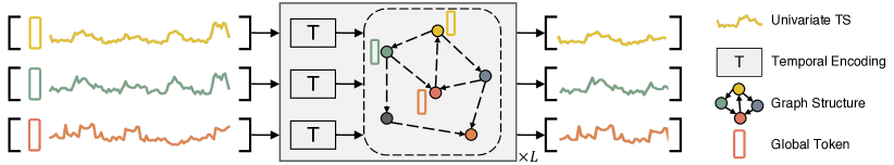
(a) Series-aware framework (Ours)

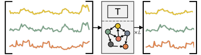
(b) Series-mixing framework

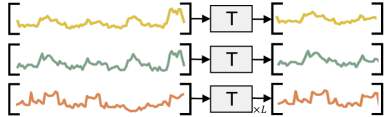
(c) Series-independent framework

Figure 1: Illustration of three different ways of modeling series dependencies: (a) The proposed series-aware framework. Prior to the original input tokens into the Transformer encoder, we incorporate learnable global tokens to capture the intrinsic features of each series. The embedding tokens are processed through multiple SageFormer layers, where temporal encoding and graph aggregation are performed iteratively. (b) The series-mixing framework amalgamates all series at once and employs temporal encoding or GNNs to process them. (c) The series-independent framework handles each series separately, improving the learning of unique temporal patterns for different series.

In this paper, we delve into the intricacies of inter-series dependencies in long-term MTS forecasting problems. We introduce the series-aware framework designed to precisely model inter-series dependencies, as illustrated by Fig. 1a. This framework forms the foundation upon which we develop the Series-Aware Graph-Enhanced Transformer (SageFormer), a series-aware Transformer model enhanced with graph neural networks (GNN). Learning with graph structures, we aim to distinguish series using interactable global tokens and improve the modeling ability for diverse temporal patterns across series through graph aggregation. The series-aware framework can function as a universal extension for Transformer-based structures, better utilizing both intra- and inter-series dependencies and achieving superior performance without greatly affecting model complexity. We contend that the proposed SageFormer addresses two challenges in long-term inter-series dependencies modeling:

1. How can diverse temporal patterns among series be effectively represented?

The series-aware framework augments the conventional series-independent framework. Our enhancement involves the introduction of several globally interactable tokens placed ahead of the input tokens. These global tokens are adept at capturing overarching information for each variable through intra-series interactions, employing mechanisms such as self-attention, CNNs, and the like. Moreover, they play a pivotal role in enabling information exchange between sequences via inter-series interactions. The global tokens enables series-aware framework to learn not only individual series’ temporal patterns but also focus on dependencies between different series, thereby enhancing diversity and effectively addresses the limitations associated with the series-independent framework, as detailed in section IV-E.

1. How can the impact of redundant information across series be avoided?

We propose using sparsely connected graph structures to reduce the impact of redundant information in unrelated series. In MTS forecasting, not all information is useful due to redundancy in time and series dimensions [16]. To evaluate model effectiveness with sparse data, we designed Low-rank datasets with varying series numbers (see Section IV-E). Our model’s performance remains stable as series dimensions increase, utilizing low-rank properties effectively. In contrast, the series-mixing method suffers from prediction deterioration as series dimensions grow.

Our contributions are threefold: First, we unveil the series-aware framework, a novel extension for Transformer-based models, utilizing global tokens to effectively exploit inter-series dependencies without adding undue complexity. Next, we introduce SageFormer, a series-aware Transformer tailored for long-term MTS forecasting. Unlike existing models, SageFormer excels in capturing both intra- and inter-series dependencies. Finally, extensive experiments on both real-world and synthetic datasets verify the effectiveness and superiority of SageFormer.

II Related Works

II-A Multivariate Time Series Forecasting

MTS forecasting models can generally be categorized into statistical and deep models. Many forecasting methods begin with traditional tools such as the Vector Autoregressive model and the Vector Autoregressive Moving Average [17, 18]. These typical statistical MTS forecasting models assume linear dependencies between series and values. With the advancement of deep learning, various deep models have emerged and often demonstrate superior performance compared to their statistical counterparts. Temporal Convolutional Networks [19, 20] and DeepAR [21] consider MTS data as sequences of vectors, employing CNNs and RNNs to capture temporal dependencies.

II-B Transformers for long-term MTS Forecasting

Recently, Transformer models with self-attention mechanisms have excelled in various fields [22, 23, 24, 25]. Numerous studies aim to enhance Transformers for long-term MTS forecasting by addressing their quadratic complexity. Notable approaches include Informer [5], introducing ProbSparse self-attention and distilling techniques; Autoformer [9], incorporating decomposition and auto-correlation concepts; FEDformer [10], employing a Fourier-enhanced structure; and Pyraformer [26], implementing pyramidal attention modules. PatchTST [14] divides each series into patches and uses a series-independent Transformer to model temporal patterns. While these models primarily focus on reducing temporal dependencies modeling complexity, they often overlook crucial inter-series dependencies.

II-C Inter-series dependencies for MTS Forecasting

Several methods have been proposed to explicitly enhance inter-series dependencies in MTS forecasting. LSTnet [6] employs CNN for inter-series dependencies and RNN for temporal dependencies. GNN-based models [27, 28, 29, 30], such as MTGNN [30], utilize temporal and graph convolution layers to address both dependencies. STformer [31] flattens multivariate time series into a 1D sequence for Transformer input, while Crossformer [12] employs dimension-segment-wise embedding and a two-stage attention layer for efficient temporal and inter-series dependencies capture respectively. Although there exist several works showing the effectiveness of temporal convolutions to model long-range dependencies [32, 33], most traditional CNN and GNN-based methods still focus on short-term prediction and struggle to capture long-term temporal dependencies. STformer [31] and Crossformer [12] extend 1-D attention to 2-D, but they fail to reveal the relationships between series explicitly. Unlike the methods mentioned above, our proposed framework serves as a general framework that can be applied to various Transformer-based models, utilizing graph structures to enhance their ability to represent inter-series dependencies.

III Methodology

III-A Problem Definition

In this paper, we concentrate on long-term MTS forecasting tasks. Let $\mathbf{x}_{t}\in\mathbb{R}^{C}$ denote the value of $C$ series at time step $t$. Given a historical MTS sample $\mathbf{X}_{t}=\left[\mathbf{x}_{t},\mathbf{x}_{t+1},\cdots,\mathbf{x}_{t+H-1}\right]\in\mathbb{R}^{C\times H}$ with length $H$, the objective is to predict the next $T$ steps of MTS values $\mathbf{Y}_{t}=\left[\mathbf{x}_{t+L},\cdots,\mathbf{x}_{t+L+T-1}\right]\in\mathbb{R}^{C\times T}$. The aim is to learn a mapping $f(\cdot):\mathbf{X}_{t}\rightarrow\mathbf{Y}_{t}$ using the proposed model (we omit the subscript $t$ when it does not cause ambiguity).

We employ graphs to represent inter-series dependencies in MTS and briefly overview relevant graph-related concepts. From a graph perspective, different series in MTS are considered nodes, and relationships among series are described using the graph adjacency matrix. Formally, the MTS data can be viewed as a signal set $\mathcal{G}=\left\{\mathcal{V},\mathbf{X}_{t},\mathbf{A}\right\}$. The node set $\mathcal{V}$ contains $C$ series of MTS data and $\mathbf{A}\in\mathbb{R}^{C\times C}$ is a weighted adjacency matrix. The entry $a_{ij}$ indicates the dependencies between series $i$ and $j$. If they are not dependent, $a_{ij}$ equals zero. The main symbols used in the paper and their meanings are detailed in Table I.

III-B Overview

The series-aware framework, as illustrated in Algorithm 1, is designed to forecast MTS data. The workflow mainly consists of two components: the generation of global tokens, and an iterative message passing procedure. Within the message passing mechanism, contemporary architectures can be utilized for both inter-series and intra-series information propagation.

SageFormer is an instantiation of the Series-Aware framework. It effectively employs GNNs to model inter-series dependencies, while leveraging Transformers to capture intra-series dependencies. Thus, it ensures the model comprehensively grasps the underlying dynamics of the series-aware setup. The overall structure adheres to a Transformer encoder design, and replaces the conventional Transformer decoder with a more efficient linear decoder head ($\operatorname{ForecastingHead}$), as supported by the literature [13, 14, 34]. With its unique combination of GNNs and Transformers, SageFormer emerges as a promising solution for capturing and modeling the essence of intra- and inter-series relations.

TABLE I: Table of Notations

Symbol	Description
$\mathrm{C}$	Number of series in MTS data
$H$	Historical input length
$T$	Predictive horizontal length
$\mathbf{x}_{t}\in\mathbb{R}^{C}$	The value of $C$ series at time step $t$
$\mathbf{X}_{t}\in\mathbb{R}^{C\times L}$	A historical MTS sample with length $L$
$\mathbf{Y}_{t}\in\mathbb{R}^{C\times T}$	The next $T$ steps of MTS values to be predicted
$f(\cdot)$	Mapping function from $\mathbf{X}_{t}$ to $\mathbf{Y}_{t}$
$\mathcal{G}=\left\{\mathcal{V},\mathbf{X}_{t},\mathbf{A}\right\}$	MTS data viewed from a graph perspective
$\mathcal{V}$	Node set containing $C$ series of MTS data
$\mathbf{A}\in\mathbb{R}^{C\times C}$	Weighted adjacency matrix
$a_{ij}$	Entry indicating the dependencies between series $i$ and $j$
$\mathcal{X}^{(l)}\in\mathbb{R}^{C\times(N+M)\times D}$	Embedding with global tokens of $l$-th layer
$L$	Number of encoder layers
$\mathrm{TEB}$	Transformer Encoding Block
$\mathrm{GNN}$	Graph Neural Network
$\operatorname{ForecastingHead}$	Decoder head that produces the predictions

Algorithm 1 Series-aware Framework’s Workflow

1:The input MTS history $\mathbf{X}$

2:The predicted MTS future $\mathbf{Y}$

3:$\mathcal{X}^{(0)}\leftarrow\operatorname{GlobalEembedding}(\mathbf{X})$ $\triangleright$ global tokens

4:for $c=1,\dots,C$ do

5:     $\mathcal{X}^{(1)}_{:,c,:}\leftarrow\mathrm{IntraSeries}\left(\mathcal{X}^{(0)}_{:,c,:}\right)$

6:end for

7:for $l=2,\dots,L-1$ do$\triangleright$ iterative message passing

8:     for $m=1,...,M$ do

9:         $\widehat{\mathcal{X}}^{(l)}_{:,m,:}\leftarrow\mathrm{InterSeries}\left(\mathcal{X}^{(l)}_{:,m,:}\right)$ $\triangleright$ series-aware

10:     end for

11:     for $c=1,\dots,C$ do

12:         $\mathcal{X}^{(l+1)}_{c,:,:}\leftarrow\mathrm{IntraSeries}\left(\widehat{\mathcal{X}}^{(l)}_{c,:,:}\right)$ $\triangleright$ temporal

13:     end for

14:end for

15:$\hat{\mathcal{X}}\leftarrow\left\{\mathcal{X}^{(L)}_{m,:,:}|m>M\right\}$

16:return $Y\leftarrow\mathrm{ForecastingHead}\left(\hat{\mathcal{X}}\right)$

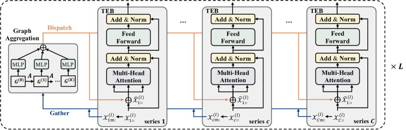
Figure 2: Illustration of the iterative message-passing process in SageFormer. Each layer begins with graph aggregation, where global tokens from all series are gathered and processed by the multi-hop GNN component (leftmost rectangle). Graph-enhanced global tokens are then dispatched to their original series and encoded by TEB. The weights of each TEB are shared among all series.

III-C Series-aware Global Tokens

The traditional approach in Transformers involves obtaining input tokens by projecting point-wise or patch-wise split input time-series [5, 10, 14]. This is executed with the intention that these tokens embody local semantic information, which can then be examined for their mutual connections through self-attention mechanisms.

Our methodology introduces a pivotal innovation: the integration of global tokens to enhance series awareness. Drawing from the concept of the class token in Natural Language Processing models [23] and Vision Transformer [35], we prepend learnable tokens for each series to encapsulate their corresponding global information. As detailed in Section III-E, we leverage these global tokens to capture inter-series dependencies, thereby augmenting the series awareness of each sub-series, a novel approach that distinguishes our method.

In accordance with PatchTST [14], the input MTS $\mathbf{X}\in\mathbb{R}^{C\times H}$ is reshaped into overlapped patches $\mathcal{X}_{p}=\{\mathbf{X}_{1},\cdots,\mathbf{X}_{C}\}\in\mathbb{R}^{C\times N\times P}$. Here P is the subsequence patch length, and $N=\left\lfloor(H-P)/S\right\rfloor+2$ denotes the number of patches. Additionally, $S$ indicates the non-overlapping length between adjacent patches. $\mathbf{X}_{c}=\{\mathbf{x}_{c}^{1},\cdots,\mathbf{x}_{c}^{N}\}\in\mathbb{R}^{N\times P}$ represents the patched sequence for series $c$. To facilitate the processing within the Transformer encoding blocks (TEB), each patch in $\mathcal{X}_{p}$ is projected into a consistent latent space of size $D$ using a trainable linear projection ($\mathbf{E}_{proj}\in\mathbb{R}^{P\times D}$), as detailed in Equation 1.

$M$ learnable embeddings (global tokens) $\mathbf{g}_{i}\in\mathbb{R}^{D}$ are added before the patched sequences, representing each series’ global information enhanced by self-attention, resulting in an effective input token sequence length of $M+N$. The prepended global tokens are designed to facilitate interaction across series. Positional information is enhanced via 1D learnable additive position embeddings $\mathbf{E}_{pos}$. The final embedding of input MTS sample $\mathbf{X}$ is $\mathcal{X}^{(0)}\in\mathbb{R}^{C\times(M+N)\times D}$, where

$$\mathcal{X}^{(0)}_{c,:,:}=\left[\mathbf{g}_{1};\cdots;\mathbf{g}_{M};\mathbf{x}^{1}_{c}\mathbf{E}_{proj};\cdots;\mathbf{x}^{N}_{c}\mathbf{E}_{proj}\right]+\mathbf{E}_{pos}.$$ (1)

III-D Graph Structure Learning

In SageFormer, the adjacency matrix is learned end-to-end, enabling the capture of relationships across series without the necessity of prior knowledge. In MTS forecasting, we posit that inter-series dependencies are inherently unidirectional. For example, while the power load may influence oil temperature, the converse isn’t necessarily valid. Such directed relationships are represented within the graph structure we derive. It’s worth noting that many time series lack an intrinsic graph structure or supplementary auxiliary data. However, our methodology is adept at deducing the graph structure solely from the data, obviating the need for external inputs. This attribute enhances its versatility and wide-ranging applicability.

Specifically, the entire graph structure learning module can be described by the following equations:

$$\mathbf{M}_{1} =\operatorname{act}(\mathbf{E}\mathbf{\Theta}_{1});\ \mathbf{M}_{2}=\operatorname{act}(\mathbf{E}\mathbf{\Theta}_{2})$$ (2)

$$\mathbf{A}^{\prime} =\operatorname{Relu}(\mathbf{M}_{1}\mathbf{M}_{2}^{T}-\mathbf{M}_{2}\mathbf{M}_{1}^{T})$$ (3)

Node embeddings of series are learned through randomly initialized $\mathbf{E}\in\mathbb{R}^{C\times D_{g}}$, where $D_{g}$ is the number of features in node embeddings. Subsequently, $\mathbf{E}$ is transformed into $\mathbf{M}\in\mathbb{R}^{C\times D_{g}}$ using trainable parameters $\mathbf{\Theta_{1}},\mathbf{\Theta_{2}}\in\mathbb{R}^{D_{g}\times D_{g}}$, with the nonlinear activation function $\operatorname{act}$ (Equation 2). Following the approach of MTGNN [30], Equation 3 is employed to learn unidirectional dependencies. For each node, the top $K$ nearest nodes are identified as neighbors from $\mathbf{A}^{\prime}$. Weights of nodes that aren’t connected are set to zero. This process results in the final sparse adjacency matrix $\mathbf{A}\in\mathbb{R}^{C\times C}$ of the uni-directional graph $\mathcal{G}$.

TABLE II: The statistics of the six mainstream datasets.

Datasets	Traffic	Electricity	Weather	Exchange	ILI	ETTh1/ETTh2	ETTm1/ETTm2
Number of Series	862	321	21	8	7	7	7
Timesteps	17,544	26,304	52,696	7588	966	17,420	69,680
Temporal Granularity	1 hour	1 hour	10 mins	1 day	1 week	1 hour	15 mins

III-E Iterative Message Passing

The embedding tokens (outlined in Section III-C) are processed by SageFormer encoder layers, where temporal encoding and graph aggregation are conducted iteratively (Fig. 2). This approach aims to disseminate the global information gathered during the GNN phase among all tokens within each series. As a result, the model captures both intra- and inter-series dependencies through iterative message passing.

Graph Aggregation

The graph aggregation phase aims to fuse each series’ information with its neighbors’ information, thereby enhancing each series’ representation with related patterns. For each series in the $l$-th layer, we take the first $M$ embeddings as the global tokens of layer $l$: $\mathbf{G}_{i}^{(l)}\leftarrow\mathcal{X}^{(l)}_{:,i,:}\in\mathbb{R}^{C\times D},\,i\leq M$. The global tokens of layer $l$ are gathered from all series and passed into the GNN for graph aggregation. For simplicity, we employ the same model as [27, 30] for graph aggregation:

$$\widehat{\mathbf{G}}_{i}=\sum_{d=0}^{D}\tilde{\mathbf{A}}^{d}\mathbf{G}_{i}\mathbf{W}_{d},\ i\leq M$$ (4)

Equation 4 represents multi-hop information fusion on the graph, where $D$ denotes the depth of graph aggregation and $\tilde{\mathbf{A}}$ is the graph Laplacian matrix. Each of the embeddings $\widehat{\mathbf{G}}_{i}$ is dispatched to its original series and then concatenated with series tokens, resulting in graph-enhanced embeddings $\widehat{\mathcal{X}}^{(l)}$.

Temporal Encoding

The graph-enhanced embeddings are later processed by Transformer components (Transformer[22], Informer [5], FEDformer [10], etc.). We choose the vanilla Transformer encoder blocks [22] as our backbone. The output of the TEB functions as input token-level embeddings for the following encoding layer. Previously aggregated information from the GNN is disseminated to other tokens within each series via self-attention, enabling access to related series information. This process enhances the expressiveness of our model compared to series-independent models.

IV Experiments

IV-A Experimental Setup

Datasets

To evaluate our proposed series-aware framework and SageFormer, extensive experiments have been conducted on six mainstream real-world datasets, including Weather, Traffic, Electricity, ILI(Influenza-Like Illness), and four ETT(Electricity Transformer Temperature) datasets and two synthetic datasets (see section IV-E). The statistics of these multivariate datasets are shown in Table II. Among all datasets, Traffic and Electricity have more series, which can better reflect the effectiveness of the proposed method. The details are described below:

1. The Traffic dataset contains data from 862 sensors installed on highways in the San Francisco Bay Area, measuring road occupancy. This dataset is recorded on an hourly basis over two years, resulting in a total of 17,544 time steps.

2. The Electricity Consumption Load (Electricity) dataset records the power usage of 321 customers. The data is logged hourly over a two-year period, amassing a total of 26,304 time steps.

3. The Weather dataset is a meteorological collection featuring 21 variates, gathered in the United States over a four-year span.

4. The Exchange dataset details the daily foreign exchange rates of eight different countries, including Australia, British, Canada, Switzerland, China, Japan, New Zealand and Singapore ranging from 1990 to 2016.

5. The Influenza-Like Illness (ILI) dataset is maintained by the United States Centers for Disease Control and Prevention. It collates patient information on a weekly basis for a period spanning from 2002 to 2021.

6. The Electricity Transformers Temperature (ETT) datasets are procured from two electricity substations over two years. They provide a summary of load and oil temperature data across seven variates. For ETTm1 and ETTm2, the ”m” signifies that data was recorded every 15 minutes, yielding a total of 69,680 time steps. ETTh1 and ETTh2 represent the hourly equivalents of ETTm1 and ETTm2, respectively, each containing 17,420 time steps.

Baselines and Task Settings

We compare our proposed method with nine popular models for long-term MTS forecasting problems as baselines, including three models that explicitly utilize inter-series dependencies: Crossformer[12], MTGNN[30], and LSTnet[6]; two series-independent neural models: DLinear[13] and PatchTST[14]; and four series-mixing transformer-based models: Transformer[22], Informer[5], Autoformer[9], and Non-stationary Transformer[36].

All baselines are reproduced using the original paper’s configuration or the official code. However, the only exception is that we standardize the look-back window across all models to 36 for the ILI dataset and 96 for the remaining datasets to ensure a fair comparison. Consequently, some discrepancies may exist between our input-output setting and those reported in the referenced papers. We exclude traditional time series forecasting models (such as ARIMA, LSTM) from our baselines, as Transformer-based models have been demonstrated to outperform these in long-term forecasting tasks [5].

TABLE III: Long-Term Forecasting Task Results.

Models		SageFormer		Crossformera		MTGNNa		LSTneta		PatchTSTb		DLinearb		Stationaryc		Autoformerc		Informerc		Transformerc
		(Ours)		[12]*		[30]*		[6]*		[14]*		[13]*		[36]		[9]		[5]		[22]
Metric		MSE	MAE	MSE	MAE	MSE	MAE	MSE	MAE	MSE	MAE	MSE	MAE	MSE	MAE	MSE	MAE	MSE	MAE	MSE	MAE
Traffic	96	0.408	0.271	0.544	0.307	0.574	0.312	0.711	0.432	0.450	0.287	0.650	0.396	0.612	0.338	0.613	0.388	0.719	0.391	0.644	0.354
	192	0.421	0.279	0.566	0.315	0.587	0.315	0.722	0.441	0.456	0.292	0.598	0.370	0.613	0.340	0.616	0.382	0.696	0.379	0.662	0.365
	336	0.438	0.283	0.571	0.314	0.594	0.318	0.741	0.451	0.471	0.297	0.605	0.373	0.618	0.328	0.622	0.337	0.777	0.420	0.661	0.361
	720	0.477	0.308	0.599	0.313	0.612	0.322	0.768	0.474	0.509	0.317	0.645	0.394	0.653	0.355	0.660	0.408	0.864	0.472	0.677	0.370
	Avg	0.436	0.285	0.570	0.312	0.592	0.317	0.736	0.450	0.472	0.298	0.625	0.383	0.624	0.340	0.628	0.379	0.764	0.416	0.661	0.363
Electricity	96	0.147	0.246	0.213	0.300	0.243	0.342	0.382	0.452	0.175	0.266	0.197	0.282	0.169	0.273	0.201	0.317	0.274	0.368	0.259	0.358
	192	0.161	0.259	0.290	0.351	0.298	0.364	0.401	0.482	0.184	0.274	0.196	0.285	0.182	0.286	0.222	0.334	0.296	0.386	0.265	0.363
	336	0.180	0.279	0.348	0.389	0.368	0.396	0.419	0.477	0.200	0.290	0.209	0.301	0.200	0.304	0.231	0.338	0.300	0.394	0.273	0.369
	720	0.213	0.309	0.405	0.425	0.422	0.410	0.556	0.565	0.240	0.322	0.245	0.333	0.222	0.321	0.254	0.361	0.373	0.439	0.291	0.377
	Avg	0.175	0.273	0.314	0.366	0.333	0.378	0.440	0.494	0.200	0.288	0.212	0.300	0.193	0.296	0.227	0.338	0.311	0.397	0.272	0.367
Weather	96	0.162	0.206	0.162	0.232	0.189	0.252	0.682	0.594	0.175	0.216	0.196	0.255	0.173	0.223	0.266	0.336	0.300	0.384	0.399	0.424
	192	0.211	0.250	0.208	0.277	0.235	0.299	0.755	0.652	0.219	0.256	0.237	0.296	0.245	0.285	0.307	0.367	0.598	0.544	0.566	0.537
	336	0.271	0.294	0.265	0.320	0.295	0.359	0.782	0.683	0.277	0.297	0.283	0.335	0.321	0.338	0.359	0.395	0.578	0.523	0.631	0.582
	720	0.345	0.343	0.388	0.391	0.440	0.481	0.851	0.757	0.353	0.346	0.345	0.381	0.414	0.410	0.419	0.428	1.059	0.741	0.849	0.685
	Avg	0.247	0.273	0.256	0.305	0.290	0.348	0.768	0.672	0.256	0.279	0.265	0.317	0.288	0.314	0.338	0.382	0.634	0.548	0.611	0.557
ETTm1	96	0.324	0.362	0.361	0.402	0.428	0.446	1.339	0.913	0.319	0.361	0.345	0.372	0.386	0.398	0.505	0.475	0.672	0.571	0.701	0.609
	192	0.368	0.387	0.403	0.440	0.457	0.469	1.542	1.009	0.370	0.389	0.380	0.389	0.459	0.444	0.553	0.496	0.795	0.669	0.829	0.676
	336	0.401	0.408	0.551	0.535	0.579	0.562	1.920	1.234	0.406	0.410	0.413	0.413	0.495	0.464	0.621	0.537	1.212	0.871	1.024	0.783
	720	0.457	0.441	0.720	0.649	0.798	0.671	2.987	1.669	0.461	0.444	0.474	0.453	0.585	0.516	0.671	0.561	1.166	0.823	1.189	0.843
	Avg	0.388	0.400	0.509	0.507	0.566	0.537	1.947	1.206	0.389	0.401	0.403	0.407	0.481	0.456	0.588	0.517	0.961	0.734	0.936	0.728
ETTm2	96	0.173	0.255	0.253	0.347	0.289	0.364	0.723	0.655	0.177	0.261	0.193	0.292	0.192	0.274	0.255	0.339	0.365	0.453	0.515	0.534
	192	0.239	0.299	0.421	0.483	0.456	0.492	1.285	0.932	0.241	0.303	0.284	0.362	0.280	0.339	0.281	0.340	0.533	0.563	1.424	0.892
	336	0.299	0.338	1.276	0.805	1.432	0.812	3.064	1.556	0.302	0.343	0.369	0.427	0.334	0.361	0.339	0.372	1.363	0.887	1.183	0.829
	720	0.395	0.395	3.783	1.354	2.972	1.336	5.484	1.978	0.401	0.403	0.554	0.522	0.417	0.413	0.433	0.432	3.379	1.338	2.788	1.237
	Avg	0.277	0.322	1.433	0.747	1.287	0.751	2.639	1.280	0.280	0.328	0.350	0.401	0.306	0.347	0.327	0.371	1.410	0.810	1.478	0.873
ETTh1	96	0.377	0.397	0.421	0.448	0.522	0.490	1.654	0.982	0.372	0.396	0.386	0.400	0.513	0.491	0.449	0.459	0.865	0.713	0.780	0.685
	192	0.423	0.425	0.534	0.515	0.542	0.536	1.999	1.218	0.439	0.433	0.437	0.432	0.534	0.504	0.500	0.482	1.008	0.792	0.906	0.755
	336	0.459	0.445	0.656	0.581	0.736	0.643	2.655	1.369	0.468	0.456	0.481	0.459	0.588	0.535	0.521	0.496	1.107	0.809	0.980	0.797
	720	0.465	0.466	0.849	0.709	0.916	0.750	2.143	1.380	0.491	0.486	0.519	0.516	0.643	0.616	0.514	0.512	1.181	0.865	1.008	0.800
	Avg	0.431	0.433	0.615	0.563	0.679	0.605	2.113	1.237	0.443	0.443	0.456	0.452	0.570	0.537	0.496	0.487	1.040	0.795	0.919	0.759
ETTh2	96	0.286	0.338	1.142	0.772	1.843	0.911	3.252	1.604	0.302	0.346	0.333	0.387	0.476	0.458	0.346	0.388	3.755	1.525	2.590	1.282
	192	0.368	0.394	1.784	1.022	2.439	1.325	5.122	2.309	0.379	0.398	0.477	0.476	0.512	0.493	0.456	0.452	5.602	1.931	6.464	2.102
	336	0.413	0.429	2.644	1.404	2.944	1.405	4.051	1.742	0.418	0.431	0.594	0.541	0.552	0.551	0.482	0.486	4.721	1.835	5.851	1.970
	720	0.427	0.449	3.111	1.501	3.244	1.592	5.104	2.378	0.423	0.440	0.831	0.657	0.562	0.560	0.515	0.511	3.647	1.625	3.063	1.411
	Avg	0.374	0.403	2.170	1.175	2.618	1.308	4.382	2.008	0.381	0.404	0.559	0.515	0.526	0.516	0.450	0.459	4.431	1.729	4.492	1.691
Exchange	96	0.082	0.200	0.256	0.367	0.289	0.388	0.593	0.711	0.087	0.205	0.088	0.218	0.111	0.237	0.197	0.323	0.847	0.752	0.527	0.566
	192	0.175	0.298	0.469	0.508	0.441	0.498	1.164	1.047	0.183	0.305	0.176	0.315	0.219	0.335	0.300	0.369	1.204	0.895	0.942	0.737
	336	0.331	0.416	0.901	0.741	0.934	0.774	1.544	1.196	0.321	0.410	0.313	0.427	0.421	0.476	0.509	0.524	1.672	1.036	1.485	0.946
	720	0.826	0.683	1.398	0.965	1.478	1.037	3.425	1.833	0.825	0.680	0.839	0.695	1.092	0.769	1.447	0.941	2.478	1.310	2.588	1.341
	Avg	0.354	0.399	0.756	0.645	0.786	0.674	1.681	1.197	0.354	0.400	0.354	0.414	0.461	0.454	0.613	0.539	1.550	0.998	1.386	0.898
ILI	24	2.180	0.858	3.110	1.179	4.265	1.387	4.975	1.660	2.066	0.854	2.398	1.040	2.294	0.945	3.483	1.287	5.764	1.677	4.644	1.434
	36	2.214	0.877	3.429	1.222	4.777	1.496	5.322	1.659	2.173	0.881	2.646	1.088	1.825	0.848	3.103	1.148	4.755	1.467	4.533	1.442
	48	2.068	0.876	3.451	1.203	5.333	1.592	5.425	1.632	2.032	0.892	2.614	1.086	2.010	0.900	2.669	1.085	4.763	1.469	4.758	1.469
	60	1.991	0.898	3.678	1.255	5.070	1.552	5.477	1.675	1.987	0.899	2.804	1.146	2.178	0.963	2.770	1.125	5.264	1.564	5.199	1.540
	Avg	2.113	0.877	3.417	1.215	4.861	1.507	5.300	1.657	2.065	0.882	2.616	1.090	2.077	0.914	3.006	1.161	5.137	1.544	4.784	1.471
$1^{\text{st}}$ Count		55		3		0		0		12		2		2		0		0		0

• We compare extensive competitive models under different prediction lengths (96, 192, 336, 720). The input sequence length is set to 36 for the ILI dataset and 96 for the others. Avg is averaged from all four prediction lengths. Bold/underline indicates the best/second.

• a marks the models explicitly utilizing inter-series dependencies; b marks series-independent neural models; c marks series-mixing transformer-based models.

• $\ast$ means that there are some mismatches between our input-output setting and their papers. We adopt their official codes and only change the length of input and output sequences for a fair comparison.

TABLE IV: Performance Promotion by Applying the Proposed Framework to Transformer and Its Variants.

Dataset		Transformer		+ Series-aware 2		Informer 3		+ Series-aware		FEDformer		+ Series-aware
Metric		MSE	MAE	MSE	MAE	MSE	MAE	MSE	MAE	MSE	MAE	MSE	MAE
Traffic	96	0.644	0.354	0.526	0.281	0.587	0.366	0.561	0.318	0.719	0.391	0.672	0.382
	192	0.662	0.365	0.536	0.287	0.604	0.373	0.572	0.320	0.696	0.379	0.688	0.369
	336	0.661	0.361	0.553	0.296	0.621	0.383	0.582	0.321	0.777	0.420	0.708	0.405
	720	0.677	0.370	0.581	0.306	0.626	0.382	0.598	0.312	0.864	0.472	0.761	0.428
	Avg	0.661	0.362	0.549	0.293	0.610	0.376	0.578	0.318	0.764	0.416	0.707	0.396
Electricity	96	0.259	0.358	0.186	0.272	0.193	0.308	0.182	0.278	0.274	0.368	0.188	0.275
	192	0.265	0.363	0.188	0.275	0.201	0.315	0.191	0.285	0.296	0.386	0.212	0.311
	336	0.273	0.369	0.203	0.293	0.214	0.329	0.206	0.313	0.300	0.394	0.223	0.327
	720	0.291	0.377	0.234	0.320	0.246	0.355	0.248	0.345	0.373	0.439	0.267	0.361
	Avg	0.272	0.367	0.202	0.290	0.214	0.327	0.207	0.305	0.311	0.397	0.223	0.319
Weather	96	0.399	0.424	0.189	0.252	0.217	0.296	0.208	0.276	0.300	0.384	0.178	0.224
	192	0.566	0.537	0.235	0.299	0.276	0.336	0.249	0.312	0.598	0.544	0.226	0.262
	336	0.631	0.582	0.295	0.359	0.339	0.380	0.296	0.322	0.578	0.523	0.287	0.305
	720	0.849	0.685	0.440	0.481	0.403	0.428	0.385	0.382	1.059	0.741	0.384	0.423
	Avg	0.611	0.557	0.290	0.348	0.309	0.360	0.285	0.323	0.634	0.548	0.269	0.304
ETTh1	96	0.780	0.685	0.384	0.403	0.376	0.419	0.377	0.408	0.865	0.713	0.578	0.512
	192	0.906	0.755	0.435	0.433	0.420	0.448	0.431	0.440	1.008	0.792	0.669	0.558
	336	0.980	0.797	0.479	0.459	0.459	0.465	0.455	0.456	1.107	0.809	0.699	0.592
	720	1.008	0.800	0.538	0.528	0.506	0.507	0.467	0.462	1.181	0.865	0.745	0.644
	Avg	0.919	0.759	0.459	0.456	0.440	0.460	0.433	0.442	1.040	0.795	0.673	0.577

• We compare base models and the proposed series-aware framework under different prediction lengths (96, 192, 336, 720). The input sequence length is set to 512 for all datasets. Bold indicates the better.

• This model diverges from SageFormer in that only the latter employs patching to generate temporal tokens.

• The inconsistency between the Informer results in Table III and Table IV arises because of different input history lengths.

Implementation details

For model training and evaluation, we adopt the same settings as in [34]. The entire dataset is rolled with a stride of 1 to generate different input-output pairs, and Train/Val/Test sets are zero-mean normalized using the mean and standard deviation of the training set. Performance is evaluated over varying future window sizes on each dataset. The past sequence length is set as 36 for ILI and 96 for the others. Mean Square Error (MSE) and Mean Absolute Error (MAE) serve as evaluation metrics. All experiments are conducted five times, and the mean of the metrics is reported.

We conduct all experiments five times, each implemented in PyTorch, and carried out on a single NVIDIA TITAN RTX 3090 24GB GPU. The repeated experimentation helps mitigate the effects of random variations in reported values. The look-back window size is set to 96, while the forecasting horizon ranges between 96 and 720. Model optimization is achieved through the Adam optimizer with a learning rate of $1e-4$. The models are trained for about 20 epochs, utilizing an early stop mechanism to prevent overfitting.

By default, SageFormer comprises two encoder layers, an attention head count ($H$) of 16, and a model hidden dimension ($d$) of 512. We designate the number of global tokens as $M=1$; the node embedding dimension $D_{g}$ is set to 16, the number of nearest neighbors is $K=16$, and the graph aggregation depth is $D=3$. Furthermore, we employ a patch length ($P$) of 24 and a stride ($S$) of 8, consistent with the parameters utilized in PatchTST. For the larger datasets (Traffic, Electricity), a model with three encoder layers is adopted to enhance the expressive capacity.

IV-B Main Results

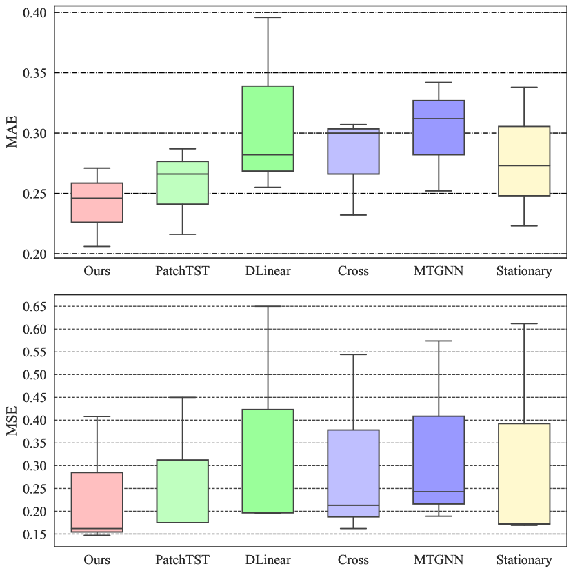
Figure 3: MAE / MSE restuls on Traffic, Electricity, and Weather datasets.

TABLE V: Model Architecture Ablations.

Datasets	Traffic				AVG	ETTh1				AVG
Prediction Lengths	96	192	336	720		96	192	336	720
SageFormer	0.408	0.421	0.438	0.477	0.436	0.377	0.423	0.459	0.465	0.431
- Graph Aggregation	0.446	0.452	0.466	0.506	0.468	0.372	0.439	0.468	0.491	0.443
- Global Tokens	0.420	0.440	0.457	0.507	0.456	0.381	0.431	0.462	0.478	0.438
- Sparse Graph	0.416	0.441	0.445	0.484	0.447	0.377	0.423	0.459	0.467	0.432
- Directed Graph	0.415	0.442	0.449	0.494	0.450	0.379	0.424	0.461	0.468	0.433

• MSE metrics are reported. -Graph Aggregation: Elimination of graph aggregation in the encoder; -Global Tokens: Graph information propagation applied to all tokens without global tokens; -Sparse Graph: Removal of the k-nearest neighbor constraint in graph structure learning; -Directed Graph: Modification of graph structure learning from directed to undirected graphs.

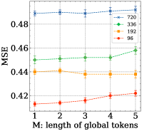
(a)

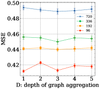
(b)

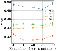
(c)

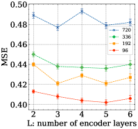
(d)

Figure 4: Evaluation on hyper-parameter impact. (a) MSE against the length of global tokens on the Traffic dataset. (b) MSE against the graph aggregation depth on the Traffic dataset. (c) MSE against the number of nearest neighbors on the Traffic dataset. (d) MSE against SageFormer encoder layers on the Traffic dataset.

Long-term forecasting results

Table III presents the forecasting results for the proposed SageFormer and other baseline models. Overall, the forecasting results presented distinctly highlight the superior performance of our proposed SageFormer when compared to other baseline models. This superior performance is consistently observed across all benchmarks and prediction lengths. Even when juxtaposed against models that explicitly model inter-series dependencies, SageFormer emerges as the more effective solution. This suggests that our method possesses a robust capability to discern and capitalize on the relationships that exist among multiple series.

Digging deeper into the results, it becomes evident that SageFormer’s prowess is even more pronounced on datasets with a higher number of variables. Specifically, on datasets such as Traffic, which has 862 predictive variables, and Electricity, with 321 predictive variables, our method offers significant enhancements. The improvements on previous state-of-the-art results are noteworthy – a 7.4% average MSE reduction for Traffic (from $0.471$ to $0.436$) and a 9.3% average MSE reduction for Electricity (from $0.193$ to $0.175$). To further elucidate this point, we’ve visualized the results of SageFormer against strong baselines for three relatively large datasets using box plots in Fig. 3. These plots reveal that SageFormer not only attains a lower error mean but also demonstrates a smaller variance compared to other models, underscoring its consistent and reliable forecasting capabilities.

Framework generality

Furthermore, our model serves as a versatile extension for Transformer-based architectures. To validate this, we apply the SageFormer framework to three prominent Transformers and report the performance enhancement of each model as Table IV. Our method consistently improves the forecasting ability of different models, demonstrating that the proposed series-aware framework is an effective, universally applicable framework. By leveraging graph structures, it can better utilize the intra- and inter-series dependencies, ultimately achieving superior predictive performance.

IV-C Ablation Study

The ablation studies were conducted to address two primary concerns: 1) the impact of graph aggregation and 2) the impact of series-aware global tokens. We designate SageFormer variants without specific components as shown in Table V.

First, the experiments validated the effectiveness of the graph structure in our MTS forecasting model. Removing the graph aggregation module from each encoder layer resulted in a substantial decline in prediction accuracy. On the Traffic dataset, the average decrease was 7.3%, and on the seven-series ETTh1 dataset, it was 2.8%, showing that graph structures enhance performance more in datasets with numerous series. Second, series-aware global tokens enhanced the model’s prediction accuracy while also reducing computational overhead. If all tokens (not just global tokens) participated in graph propagation calculations, the model’s performance would decline by 6.3% and 1.6% on the Traffic and ETTh1 datasets, respectively. Lastly, we discovered that techniques like sparse constraints and directed graphs in graph construction were more effective for larger datasets (e.g., Traffic). In comparison, they had little impact on smaller datasets’ prediction results (e.g., ETTs). This finding suggests that applying sparse constraints can mitigate the impact of variable redundancy on the model while conserving computational resources.

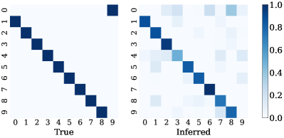
(a)

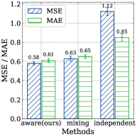
(b)

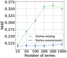
(c)

Figure 5: Evaluation on synthetic datasets. (a) The left side displays the heat map of the actual adjacency matrix, while the right side presents the inferred adjacency matrix by SageFormer, illustrating the effectiveness of our proposed method in learning the inherent graph structure.; (b) Prediction results of three different methods on the Directed Cycle Graph dataset; (c) Prediction MAE results for low-rank datasets with varying numbers of series ($N$). We selected the Nonstationary Transformer for the series-mixing method, and for the series-independent method, we chose PatchTST as a representative.

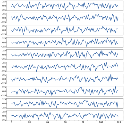
(a)

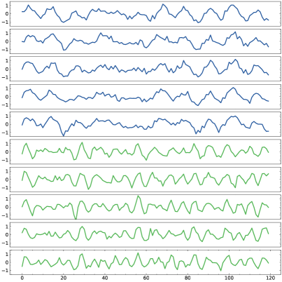
(b)

Figure 6: Visualization of 120 timesteps of (a) the Directed Cycle Graph Dataset and (b) the Low-rank Dataset.

IV-D Effect of Hyper-parameters

In this section, we examine the impact of four hyperparameters on our proposed SageFormer model: global token length, depth of graph aggregation, the number of nearest neighbors, and the depth of encoder layers. We conduct a sensitivity analysis on the Traffic dataset (Fig. 4). For each of the four tasks, SageFormer consistently delivers stable performance, regardless of the selected value.

Global token length (Fig. 4a): The model’s performance remains consistent across all prediction windows, irrespective of the value of M. To optimize computational efficiency, we set M=1. Depth of graph aggregation (Fig. 4b): The model demonstrates robust performance with varying graph aggregation depths. To balance accuracy and efficiency, we set d=3. Number of nearest neighbors (Fig. 4c): Larger k values generally yield better results, but performance declines when a fully connected graph is utilized. This suggests sequence redundancy in MTS forecasting tasks, so we select k=16. SageFormer encoder layers (Fig. 4d): Increasing the number of encoding layers results in a higher parameter count for the model and its computational time. No significant reduction is observed after the model surpasses three layers, leading us to set the model’s layers to 3.

IV-E Synthetic Datasets

The design of synthetic datasets aims to emulate specific scenarios often encountered in real-world MTS data. Through two specialized datasets, we seek to benchmark SageFormer’s performance and highlight the inherent challenges of different time series forecasting frameworks.

Directed Cycle Graph Dataset

In this section, we assess the ability of SageFormer to infer adjacency matrices using a synthetic dataset characterized by a directed cycle graph structure. The dataset contains a panel of $N=10$ time series, each of 10,000 length. Uniquely, the value of each time series $x_{i,t}$ is derived from the series indexed as $i-1\operatorname{mod}N$ with a temporal lag of $\tau=10$.

Mathematically, the generation process is:

$$x_{i,t}\sim\mathcal{N}\left(\beta x_{(i-1\operatorname{mod}N),t-10};\sigma^{2}\right),$$ (5)

where $x_{i,t}$ denotes the value of the $i$-th series at time $t$. The sampling process uses a normal distribution, denoted by $\mathcal{N}$, characterized by specific mean and variance parameters. The mean, represented as $\beta x_{(i-1\operatorname{mod}N),t-10}$, captures the scaled value from the previous series $i-1\operatorname{mod}N$ at time $t-10$. Here, $\beta$ serves as a scaling factor, and $\sigma^{2}$ delineates the allowable variance.

This cyclical generation creates a directed cycle graph in the multivariate time series adjacency matrix, as illustrated in Fig. 6a for the initial 120 timesteps. Fig. 5a juxtaposes the actual inter-series relationships with the inferences from our model, underscoring SageFormer’s adeptness at recovering these connections. Our series-aware framework, as shown in Fig. 5b, demonstrates superior performance against previous series-mixing and series-independent models, registering the most minimal MAE and MSE test losses. Notably, the series-independent approach falters significantly in this context, recording an MSE above 1. This inadequacy can be attributed to its oversight of the prominent inter-series dependencies present in this dataset. Notably, within this dataset, each sub-series mirrors white noise characteristics.

TABLE VI: Computational Complexity Per Layer of Transformer-based Models.

Methods	Encoder layer	Decoder layer	Time(s/batch)	Memory(GB)
Transformer [22]	$O(T^{2})$	$O\left(\tau(\tau+T)\right)$	$0.07\pm 0.01$	$2.39$
Informer [5]	$O(T\log T)$	$O\left(\tau(\tau+\log T)\right)$	$0.04\pm 0.04$	$2.31$
FEDformer [10]	$O(T)$	$O\left(\tau+T/2\right)$	$0.18\pm 0.03$	$3.13$
PatchTST [14]	$O(CT^{2}/P^{2})$	$O(\tau)$	$0.22\pm 0.04$	$11.44$
Crossformer [12]	$O(CT^{2}/P^{2})$	$O(C\tau(\tau+T)/P^{2})$	$0.82\pm 0.05$	$22.53$
SageFormer (ours)	$O(CT^{2}/P^{2}+C^{2})$	$O(\tau)$	$0.31\pm 0.03$	$12.42$

• $T$ denotes the length of the historical series, $\tau$ represents the length of the prediction window, $C$ is the number of series, and $P$ corresponds to the segment length of each patch.

Low-rank Dataset

To investigate how various frameworks handle sparse data, we curated several Low-rank MTS datasets with varying numbers of series. Drawing inspiration from the Discrete Sine Transformation, our datasets consist of signals synthesized from distinct sinusoids perturbed with Gaussian noise. The same sinusoids are shared among different groups of series, imbuing the datasets with the low-rank quality.

The synthetic dataset is constructed from time series, each of 10,000 length, and a variable number of series. Each series originates from a weighted combination of distinct sinusoids with specific frequencies and amplitudes. This creation process is encapsulated by:

$$x_{i}=\sum_{m=1}^{M}B_{i,m}sin\left(2\pi\omega_{\lfloor i/K\rfloor,m}t\right)+\epsilon_{i,t},$$ (6)

where $B_{i,m}$ is drawn from a normalized uniform distribution based on $\tilde{B}_{i,m}\sim U(0.4,1)$. The frequency parameter, $\omega_{\lfloor i/K\rfloor,m}$, is sampled from $U(0,0.2)$, while $\epsilon_{i,t}$ originates from $\mathcal{N}(0,0.2^{2})$. Crucially, $\omega_{\lfloor i/K\rfloor,m}$ remains consistent across series within a group, instilling the dataset’s low-rank attribute. For our experiments, the chosen parameters were $M=3$ and $K=2$.

The dataset’s distinctive low-rank feature is a consequence of the shared frequency values, $\omega_{\lfloor i/K\rfloor,m}$, among the series in a given group. This shared attribute allows the dataset to be captured with a succinct, low-dimensional representation, highlighting its low-rank nature.

Fig. 5c contrasts the prediction MAE of our method with the series-mixing approach for datasets of varying series numbers ($N$). It can be observed that the prediction performance of the series-mixing method deteriorates rapidly as the number of series increases since it encodes all series information into the same token. In contrast, the MAE of our method does not increase with the growth in the number of series, indicating that our designed approach can effectively exploit the low-rank characteristics of the dataset.

IV-F Computational Efficiency Analysis

We compared the computational efficiency of our model, SageFormer, with other Transformer-based models (Table VI). Although SageFormer’s complexity is theoretically quadratic to historical series length $T$, a large patch length $P$ in practice brings its runtime close to linear complexity models. An additional $O(C^{2})$ complexity is due to standard graph convolution operations, but techniques exist to reduce this to linear complexity [37, 38]. In the decoder part, the complexity of SageFormer is simplified to linear, owing to the streamlined design of the linear decoder head.

We also evaluated running time and memory consumption on the Traffic dataset, which has the most variables. SageFormer balances running time and memory usage well, achieving a running time of $0.31\pm 0.03$ seconds per batch and consuming $12.42$ GB of memory. This result is slightly slower compared to the PatchTST [14] model but is faster than the Crossformer [12] model. These results suggest that our proposed SageFormer model presents a competitive trade-off between efficiency and prediction accuracy.

V Conclusion

This paper presented the series-aware framework and SageFormer, a novel approach for modeling both intra- and inter-series dependencies in long-term MTS forecasting tasks. By amalgamating GNNs with Transformer structures, SageFormer can effectively capture diverse temporal patterns and harness dependencies among various series. Our model has demonstrated impressive versatility through extensive experimentation, delivering state-of-the-art performance on real-world and synthetic datasets. SageFormer thus presents a promising solution to overcome the limitations of series dependencies modeling in MTS forecasting tasks and exhibits potential for further advancements and applications in other domains involving inter-series dependencies.

We also acknowledged the limitations of our work and briefly delineated potential avenues for future research. While SageFormer achieves exceptional performance in long-term MTS forecasting, the dependencies it captures do not strictly represent causality. As a result, some dependencies may prove unreliable in practical scenarios due to the non-stationary nature of time series. Our primary focus on enhancing long-term forecasting performance has led to some degree of overlooking the interpretability of the graph structure. Moving forward, our work’s graph neural network component could be improved to learn causal relationships between variables and reduce its complexity. The framework proposed in this paper could also be applied to non-Transformer models in the future.

References

- [1] A. Zanella, N. Bui, A. Castellani, L. Vangelista, and M. Zorzi, “Internet of things for smart cities,” IEEE Internet of Things journal, vol. 1, no. 1, pp. 22–32, 2014.
- [2] S. Ren, B. Guo, K. Li, Q. Wang, Z. Yu, and L. Cao, “Coupledmuts: Coupled multivariate utility time-series representation and prediction,” IEEE Internet of Things Journal, vol. 9, no. 22, pp. 22 972–22 982, Nov 2022.
- [3] B. Huang, H. Dou, Y. Luo, J. Li, J. Wang, and T. Zhou, “Adaptive spatiotemporal transformer graph network for traffic flow forecasting by iot loop detectors,” IEEE Internet of Things Journal, vol. 10, no. 2, pp. 1642–1653, 2022.
- [4] P. K. Kashyap, S. Kumar, A. Jaiswal, M. Prasad, and A. H. Gandomi, “Towards precision agriculture: Iot-enabled intelligent irrigation systems using deep learning neural network,” IEEE Sensors Journal, vol. 21, no. 16, pp. 17 479–17 491, 2021.
- [5] H. Zhou, S. Zhang, J. Peng, S. Zhang, J. Li, H. Xiong, and W. Zhang, “Informer: Beyond efficient transformer for long sequence time-series forecasting,” in AAAI, 2021.
- [6] G. Lai, W.-C. Chang, Y. Yang, and H. Liu, “Modeling long-and short-term temporal patterns with deep neural networks,” in SIGIR, 2018.
- [7] B. Lim and S. Zohren, “Time-series forecasting with deep learning: a survey,” Philosophical Transactions of the Royal Society A, vol. 379, no. 2194, p. 20200209, 2021.
- [8] S. Li, X. Jin, Y. Xuan, X. Zhou, W. Chen, Y.-X. Wang, and X. Yan, “Enhancing the locality and breaking the memory bottleneck of transformer on time series forecasting,” in NeurIPS, 2019.
- [9] H. Wu, J. Xu, J. Wang, and M. Long, “Autoformer: Decomposition transformers with Auto-Correlation for long-term series forecasting,” in NeurIPS, 2021.
- [10] T. Zhou, Z. Ma, Q. Wen, X. Wang, L. Sun, and R. Jin, “FEDformer: Frequency enhanced decomposed transformer for long-term series forecasting,” in ICML, 2022.
- [11] J. Durbin and S. J. Koopman, Time series analysis by state space methods. OUP Oxford, 2012, vol. 38.
- [12] Y. Zhang and J. Yan, “Crossformer: Transformer utilizing cross-dimension dependency for multivariate time series forecasting,” in International Conference on Learning Representations, 2023.
- [13] A. Zeng, M. Chen, L. Zhang, and Q. Xu, “Are transformers effective for time series forecasting?” in AAAI, 2023.
- [14] Y. Nie, N. H. Nguyen, P. Sinthong, and J. Kalagnanam, “A time series is worth 64 words: Long-term forecasting with transformers,” in International Conference on Learning Representations, 2023.
- [15] L. Han, H.-J. Ye, and D.-C. Zhan, “The capacity and robustness trade-off: Revisiting the channel independent strategy for multivariate time series forecasting,” 2023.
- [16] Z. Li, Z. Rao, L. Pan, and Z. Xu, “Mts-mixers: Multivariate time series forecasting via factorized temporal and channel mixing,” arXiv preprint arXiv:2302.04501, 2023.
- [17] G. E. Box and G. M. Jenkins, “Some recent advances in forecasting and control,” J. R. Stat. Soc. (Series-C), 1968.
- [18] G. E. Box, G. M. Jenkins, G. C. Reinsel, and G. M. Ljung, Time series analysis: forecasting and control. John Wiley & Sons, 2015.
- [19] S. Bai, J. Z. Kolter, and V. Koltun, “An empirical evaluation of generic convolutional and recurrent networks for sequence modeling,” arXiv preprint arXiv:1803.01271, 2018.
- [20] R. Sen, H.-F. Yu, and I. S. Dhillon, “Think globally, act locally: A deep neural network approach to high-dimensional time series forecasting,” in NeurIPS, 2019. [Online]. Available: https://proceedings.neurips.cc/paper/2019/file/3a0844cee4fcf57de0c71e9ad3035478-Paper.pdf
- [21] D. Salinas, V. Flunkert, J. Gasthaus, and T. Januschowski, “DeepAR: Probabilistic forecasting with autoregressive recurrent networks,” Int. J. Forecast., 2020.
- [22] A. Vaswani, N. Shazeer, N. Parmar, J. Uszkoreit, L. Jones, A. N. Gomez, L. Kaiser, and I. Polosukhin, “Attention is all you need,” in NeurIPS, 2017.
- [23] J. Devlin, M.-W. Chang, K. Lee, and K. Toutanova, “Bert: Pre-training of deep bidirectional transformers for language understanding,” in NAACL-HLT, 2019.
- [24] L. Dong, S. Xu, and B. Xu, “Speech-transformer: a no-recurrence sequence-to-sequence model for speech recognition,” in 2018 IEEE international conference on acoustics, speech and signal processing (ICASSP). IEEE, 2018, pp. 5884–5888.
- [25] Z. Liu, Y. Lin, Y. Cao, H. Hu, Y. Wei, Z. Zhang, S. Lin, and B. Guo, “Swin transformer: Hierarchical vision transformer using shifted windows,” in ICCV, 2021.
- [26] S. Liu, H. Yu, C. Liao, J. Li, W. Lin, A. X. Liu, and S. Dustdar, “Pyraformer: Low-complexity pyramidal attention for long-range time series modeling and forecasting,” in ICLR, 2021.
- [27] Y. Li, R. Yu, C. Shahabi, and Y. Liu, “Diffusion convolutional recurrent neural network: Data-driven traffic forecasting,” in International Conference on Learning Representations, 2018. [Online]. Available: https://openreview.net/forum?id=SJiHXGWAZ
- [28] B. Yu, H. Yin, and Z. Zhu, “Spatio-temporal graph convolutional networks: A deep learning framework for traffic forecasting,” in Proceedings of the 27th International Joint Conference on Artificial Intelligence (IJCAI), 2018.
- [29] D. Cao, Y. Wang, J. Duan, C. Zhang, X. Zhu, C. Huang, Y. Tong, B. Xu, J. Bai, J. Tong et al., “Spectral temporal graph neural network for multivariate time-series forecasting,” Advances in neural information processing systems, vol. 33, pp. 17 766–17 778, 2020.
- [30] Z. Wu, S. Pan, G. Long, J. Jiang, X. Chang, and C. Zhang, “Connecting the dots: Multivariate time series forecasting with graph neural networks,” in Proceedings of the 26th ACM SIGKDD international conference on knowledge discovery & data mining, 2020, pp. 753–763.
- [31] J. Grigsby, Z. Wang, and Y. Qi, “Long-range transformers for dynamic spatiotemporal forecasting,” arXiv preprint arXiv:2109.12218, 2021.
- [32] A. Gu, K. Goel, and C. Ré, “Efficiently modeling long sequences with structured state spaces,” in ICLR, 2022.
- [33] M. Liu, A. Zeng, M. Chen, Z. Xu, Q. Lai, L. Ma, and Q. Xu, “Scinet: Time series modeling and forecasting with sample convolution and interaction,” Thirty-sixth Conference on Neural Information Processing Systems (NeurIPS), 2022, 2022.
- [34] H. Wu, T. Hu, Y. Liu, H. Zhou, J. Wang, and M. Long, “Timesnet: Temporal 2d-variation modeling for general time series analysis,” 2023.
- [35] A. Dosovitskiy, L. Beyer, A. Kolesnikov, D. Weissenborn, X. Zhai, T. Unterthiner, M. Dehghani, M. Minderer, G. Heigold, S. Gelly, J. Uszkoreit, and N. Houlsby, “An image is worth 16x16 words: Transformers for image recognition at scale,” in ICLR, 2021.
- [36] Y. Liu, H. Wu, J. Wang, and M. Long, “Non-stationary transformers: Rethinking the stationarity in time series forecasting,” in NeurIPS, 2022.
- [37] F. Wu, A. Souza, T. Zhang, C. Fifty, T. Yu, and K. Weinberger, “Simplifying graph convolutional networks,” in International conference on machine learning. PMLR, 2019, pp. 6861–6871.
- [38] R. Levie, F. Monti, X. Bresson, and M. M. Bronstein, “Cayleynets: Graph convolutional neural networks with complex rational spectral filters,” IEEE Transactions on Signal Processing, vol. 67, no. 1, pp. 97–109, 2018.