Optimal Surrogate Boundary Selection and Scalability Studies
for the Shifted Boundary Method on Octree Meshes

Abstract

The accurate and efficient simulation of Partial Differential Equations (PDEs) in and around arbitrarily defined geometries is critical for many application domains. Immersed boundary methods (IBMs) alleviate the usually laborious and time-consuming process of creating body-fitted meshes around complex geometry models (described by CAD or other representations, e.g., STL, point clouds), especially when high levels of mesh adaptivity are required. In this work, we advance the field of IBM in the context of the recently developed Shifted Boundary Method (SBM). In the SBM, the location where boundary conditions are enforced is shifted from the actual boundary of the immersed object to a nearby surrogate boundary, and boundary conditions are corrected utilizing Taylor expansions. This approach allows choosing surrogate boundaries that conform to a Cartesian mesh without losing accuracy or stability. Our contributions in this work are as follows: (a) we show that the SBM numerical error can be greatly reduced by an optimal choice of the surrogate boundary, (b) we mathematically prove the optimal convergence of the SBM for this optimal choice of the surrogate boundary, (c) we deploy the SBM on massively parallel octree meshes, including algorithmic advances to handle incomplete octrees, and (d) we showcase the applicability of these approaches with a wide variety of simulations involving complex shapes, sharp corners, and different topologies. Specific emphasis is given to Poisson’s equation and the linear elasticity equations.

1 Introduction

Accurate numerical solution of PDEs in and around complex objects has a significant impact on various problems in science and technology. Examples include structural analysis of complex architectures, thermal analysis over complex geometries in semiconductor electronics, and flow analysis over complex geometries in aerodynamics. Standard numerical approaches for solving these PDEs on complex geometries–finite difference method (FDM), finite element method (FEM), or finite volume method (FVM)–usually rely on the generation of body-fitted meshes. This is a major bottleneck, as creating an analysis-suitable body-fitted mesh with appropriate refinement around the complex geometry is usually time-consuming and labor-intensive. This issue is exacerbated in problems involving moving bodies or multiphysics couplings, for which deforming meshes or re-meshing is often required (sometimes at every time step).

Immersed boundary methods (IBM) alleviate the requirement of body-fitted meshes by relaxing the requirement that the mesh conforms to the object [1, 2]. IBM allowed scalable mesh generation, such as a Cartesian grid or tree-based approaches (quadtree/octree), to be deployed for simulating PDEs in and around complex objects. In this work, we concentrate on IBM in the context of FEM-based discretizations. Two main flavors of IBMs exist in this FEM context: immersogeometric analysis (IMGA, an acronym that will also refer, in what follows, to cutFEMs, the Finite Cell Method, and related approaches) and the Shifted Boundary Method (SBM).

In IMGA, the boundary representation of the body (B-rep, NURBS, or STL) is immersed into a non-body-fitted spatial discretization. The Dirichlet boundary conditions are enforced weakly on the immersed boundary surfaces using Nitsche’s method, which proved a flexible, robust and consistent approach. Interested readers are referred to [3, 4, 5, 6, 7, 8, 9, 10, 11, 12, 13, 14, 15, 16, 17, 18, 19, 20] for a detailed discussion of the mathematical formulation and practical deployment of the IMGA. The IMGA has been deployed to solve several industrial-scale complex problems [7], but suffers from the following drawbacks:

• Sliver cut-cells: The presence of sliver cut-cells (i.e., elements intersected by the object boundary that contain a very small volume of the object) may significantly deteriorate the conditioning of the algebraic system of equations. Literature suggests removing these so-formed sliver cut cells from the global assembly can prevent such deterioration in conditioning. However, this comes at the cost of accuracy. Alternatively, there have been studies demonstrating the design of preconditioners to alleviate this issue [5]. But, this has been limited to simpler operators such as Poisson’s and Stokes and requires the development of preconditioners for other PDEs. Sliver-cut cells can even produce a loss of numerical stability [15, 14].

• Load balancing: The accuracy of the IMGA is strongly contingent upon the accurate integration of cut cells. Accurate integration is performed by increasing the number of quadrature points in the cut elements. However, this leads to the issue of load balancing when performing parallel (distributed memory) simulations, as different elements end up having different amounts of computations. Furthermore, it also invalidates the tensor structure of the basis function that can be exploited to optimize the matrix and vector assembly [7, 21].

The Shifted Boundary Method (SBM) [22, 23, 24, 25, 26, 27, 28, 29, 30] alleviates the aforementioned IMGA issues. The central idea of SBM is to impose the boundary conditions not on the true boundary ($\Gamma$, see Fig. 1) but rather on a surrogate boundary in proximity of the true boundary ($\tilde{\Gamma}_{h}$, see again Fig. 1). The appropriate value of the applied boundary condition is determined by performing a Taylor series expansion. The surrogate boundary and associated shifted boundary conditions essentially transform the problem of solving the PDE in the complex original domain (denoted as $\Omega$) into a body-fitted problem in the surrogate domain (denoted as $\tilde{\Omega}_{h}$). This strategy overcomes the challenges associated with IMGA approaches. The SBM differs from the IMGA in the following aspects:

• In IMGA, the volume integration is performed over $\Omega$; whereas in SBM it is performed over $\tilde{\Omega}_{h}$. Therefore, IMGA requires a classification test (to classify if a Gauss quadrature point belongs to $\Omega$ or $\neg\Omega$) for each Gauss quadrature point in the cut elements. In contrast, SBM does not require any such test. The integration for SBM is done over all Gauss points that belong to elements within the surrogate domain $\tilde{\Omega}_{h}$.

• The integration over all Gauss points in SBM eliminates the poor conditioning of discrete operators due to the sliver cut cells arising in IMGA.

• Additionally, SBM requires no adaptive quadrature for maintaining accuracy. This obviates the need for special algorithmic treatments (like weighted partitioning [7]) to ensure load balancing. In addition, the tensor nature of the basis function is retained, which can be leveraged for performance enhancement using fast vector-matrix assembly.

SBM, therefore, appears to be a promising numerical method for solving PDEs over complex domains. In this work, we seek to address some of the relevant questions for the practical adoption of SBM—especially for simulations over complex CAD geometry domains—that are important and yet somewhat missing from the existing literature. Specifically, we address the following:

1. We extend the numerical analysis of SBM to cover cases when the true domain is a subset of the surrogate domain ($\Omega\subset\tilde{\Omega}_{h}$).

2. Different (cartesian aligned) surrogate boundaries can be constructed for a complex domain. However, some of these boundaries can be invalid, leading to disconnected surrogate domains. In this work, we codify the requirements for the set of edges/faces (in two/three dimensions) to form a valid surrogate boundary.

3. Among these possible candidate surrogate domains, we identify the optimal surrogate domain, with boundary $\tilde{\Gamma}_{h}$, that exhibits the best accuracy. We define a simple, scalable strategy to identify this optimal surrogate boundary.

4. We develop the data structures and algorithms required for the scalable deployment of SBM on adaptive, incomplete octree grids. We illustrate good scaling behavior of the framework and showcase the utility of the framework by simulating a wide variety of complex three-dimensional shapes.

The present work focuses on a particular class of PDEs, namely elliptic PDEs with applications involving diffusion (Poisson’s equation) and structural mechanics (linear elasticity) problems. The remaining paper is organized as follows: In Section 2, we describe the mathematics of the SBM along with a description of the surrogate boundary. In Section 3 we outline the definition, approach, and algorithms for identifying the optimal surrogate boundary. In Section 4 we provide the details of the algorithms for the scalable deployment of SBM. In Section 5, we illustrate this framework with extensive numerical examples in two and three dimensions. We summarize conclusions in Section 6.

2 Mathematical Formulations

2.1 The immersed variational formulation over the physical domain

Consider the non-homogeneous elliptic equation

$$\begin{split}-\Delta u&=f\quad\mathrm{on}\quad\Omega\;,\\ u&=u_{D}\quad\mathrm{on}\quad\Gamma_{D}\;,\end{split}$$ (1)

where we are interested in solving for the scalar field, $u$, over the (immersed) domain of interest $\Omega$ with boundary $\partial\Omega=\Gamma_{D}$. Defining the appropriate functional spaces for test and trial functions, the weak formulation for Poisson’s problem can be written as:

$$(\nabla u_{h},\nabla w_{h})_{\Omega_{h}}=(f,w_{h})_{\Omega_{h}}+\underbrace{\langle\nabla u_{h}\cdot\boldsymbol{n}\,,\,w_{h}\rangle_{\Gamma_{D,h}}}_{\mathrm{Consistency\;term}}+\underbrace{\langle u_{h}-u_{D}\,,\,\nabla w_{h}\cdot\boldsymbol{n}\rangle_{\Gamma_{D,h}}}_{\mathrm{Adjoint\;consistency\;term}}-\underbrace{\langle\alpha\,h^{-1}\,(u_{h}-u_{D})\,,\,w_{h}\rangle_{\Gamma_{D,h}}}_{\mathrm{Penalty\;term}},$$ (2)

where $\alpha$ is the penalty parameter for the Dirichlet boundary condition of the Poisson’s equation, and $h$ is the element size.

The last three terms in Eq. 2—consistency, adjoint consistency, and penalty terms—are the result of weakly applying the Dirichlet boundary condition as a surface integral. These extra terms result in surface integration over the true geometry, assuming that the finite element interpolation space can describe it exactly (otherwise a geometric discretization error may be introduced).

In addition to the scalar elliptic equation (Poisson equation), we also consider the equations of linear elasticity. Here, we are interested in solving for the displacement vector field, $\boldsymbol{u}$. There are three essential equations for static linear elasticity. First, the equilibrium equation (and associated boundary conditions):

$$\begin{split}\nabla\cdot\boldsymbol{\sigma}+\boldsymbol{b}&=0,\quad\mathrm{on}\quad\Omega\;,\\ \boldsymbol{u}&=\boldsymbol{u}_{D}\quad\mathrm{on}\quad\Gamma_{D}\;,\end{split}$$ (3)

where $\boldsymbol{\sigma}$ is the stress tensor, $\boldsymbol{b}$ is the body force, and again $\partial\Omega=\Gamma_{D}$. Second, the kinematics equation:

$$\boldsymbol{\varepsilon}(\boldsymbol{u})=\nabla^{s}\boldsymbol{u}=\frac{1}{2}(\nabla\boldsymbol{u}+(\nabla\boldsymbol{u})^{T})\;,$$ (4)

where $\boldsymbol{\varepsilon}(\boldsymbol{u})$ is the strain tensor and $\boldsymbol{u}$ is the displacement vector. Third, the constitutive equation:

$$\boldsymbol{\sigma}=\boldsymbol{C}\boldsymbol{\varepsilon}(\boldsymbol{u})\;,$$ (5)

where $\boldsymbol{C}$ is the elastic stiffness tensor. For isotropic materials, $\boldsymbol{C}$ can be written as a combination of Young’s modulus $E$ and Poisson’s ratio $\nu$. Integrating by parts and using Nitsche’s method to weakly enforce the Dirichlet boundary conditions, the variational form of linear elasticity can be stated as:

$$(\boldsymbol{C}\boldsymbol{\varepsilon}(\boldsymbol{u})\,,\,\nabla^{s}\boldsymbol{w}_{h})_{\Omega_{h}}=(\boldsymbol{b}\,,\,\boldsymbol{w}_{h})_{\Omega_{h}}+\underbrace{\langle(\boldsymbol{C}\boldsymbol{\varepsilon}(\boldsymbol{u}))\cdot\boldsymbol{n}\,,\,\boldsymbol{w}_{h}\rangle_{\Gamma_{D,h}}}_{\mathrm{Consistency\;term}}-\underbrace{\langle\boldsymbol{u}_{h}-\boldsymbol{u}_{D}\,,\,(\boldsymbol{C}\nabla^{s}\boldsymbol{w}_{h})\cdot\boldsymbol{n}\rangle_{\Gamma_{D,h}}}_{\mathrm{Adjoint\;consistency\;term}}-\underbrace{\langle\gamma\,h^{-1}\,(\boldsymbol{u}_{h}-\boldsymbol{u}_{D})\,,\,\boldsymbol{w}_{h}\rangle_{\Gamma_{D,h}}}_{\mathrm{Penalty\;term}}\;,$$ (6)

where the $\gamma$ is the penalty parameter for the Dirichlet boundary condition of the linear elasticity, and $h$ is the element size. The appropriate function spaces are used for the solution $\boldsymbol{u}$ and test function $\boldsymbol{w}$.

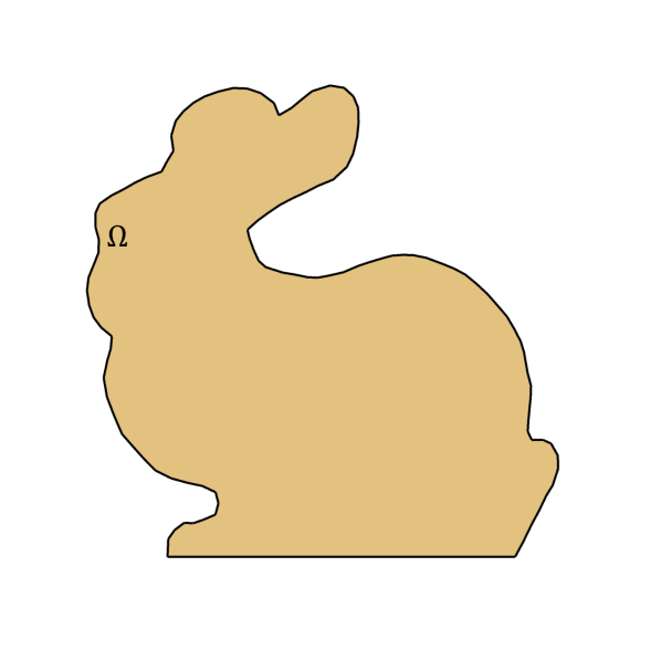
(a) $\Omega$ and $\Gamma=\partial\Omega$

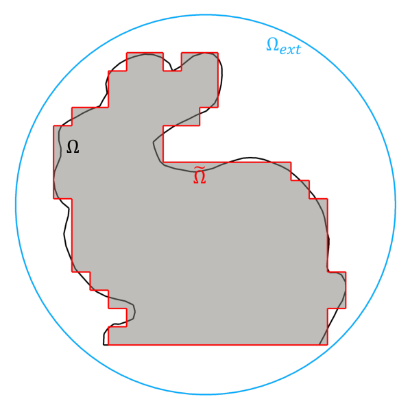
(b) $\Omega$, $\tilde{\Omega}_{h}$, and $\Omega_{\mathrm{ext}}$

Figure 1: Domain definitions for the SBM numerical analysis. The domains are classified into three types, with a corresponding color scheme: a) The physical (or true) domain $\Omega$ ($\blacksquare$), enclosed by the physical (or true) boundary $\Gamma$ (—); b) The surrogate domain $\tilde{\Omega}_{h}$ ($\blacksquare$), enclosed by the surrogate boundary $\tilde{\Gamma}_{h}$ (—); c) The extended domain $\Omega_{\mathrm{ext}}$, enclosed by the blue circle (—). The extended domain $\Omega_{\mathrm{ext}}\supset\Omega$ will only be used in mathematical proofs.

2.2 The variational formulation for the Shifted Boundary Method over the surrogate domain

The SBM introduced in [22] discretizes the governing equations on a surrogate domain $\tilde{\Omega}_{h}$ of boundary $\tilde{\Gamma}_{h}$ (rather than $\Omega$ and $\Gamma$), where $\tilde{\Omega}_{h}$ and $\tilde{\Gamma}_{h}$ do not contain any cut elements or cut element sides, respectively. For example, looking at the sketchs in Figure 1, $\Omega$ is enclosed by $\Gamma$ (the black curve), while $\tilde{\Omega}_{h}$ is enclosed by $\tilde{\Gamma}_{h}$ (the red segmented curve). The SBM resorts to a Taylor expansion of the solution variable at the surrogate boundary to shift the value of the boundary condition from $\Gamma$ to $\tilde{\Gamma}_{h}$. It is important to note that the choices of $\tilde{\Omega}_{h}$ and $\tilde{\Gamma}_{h}$ are not independent but must satisfy certain constraints, later discussed in Section 3.1. Enforcing the Dirichlet boundary condition $u=u_{D}$ on $\Gamma_{D}$ through the SBM, we deduce the following Galerkin discretization of the Poisson equation as shown below. Here, $V_{h}$ represents the appropriate function space, and subscript $h$ represents the finite dimensional analogue of operators/domains after discretization with a tesselation of size $h$.

Find $u_{h}\in V_{h}(\tilde{\Omega}_{h})$ such that, $\forall w_{h}\in V_{h}(\tilde{\Omega}_{h})$

$$(\nabla u_{h}\,,\,\nabla w_{h})_{\tilde{\Omega}_{h}} =\;(f\,,\,w_{h})_{\tilde{\Omega}_{h}}+\underbrace{\langle\nabla u_{h}\cdot\tilde{\boldsymbol{n}}\,,\,w_{h}\rangle_{\tilde{\Gamma}_{D,h}}}_{\mathrm{Consistency\;term}}+\underbrace{\langle\mathrm{S}_{h}u_{h}-u_{D}\,,\,\nabla w_{h}\cdot\tilde{\boldsymbol{n}}\rangle_{\tilde{\Gamma}_{D,h}}}_{\mathrm{Adjoint\;consistency\;term}}$$ (7)

$$\phantom{=}\;\;\;-\underbrace{\langle\alpha\,h^{-1}\,(\mathrm{S}_{h}u_{h}-u_{D})\,,\,\mathrm{S}_{h}w_{h}\rangle_{\tilde{\Gamma}_{D,h}}}_{\mathrm{Penalty\;term}}\,,$$ (8)

where $\mathrm{S}_{h}v$ is the boundary shift operator:

$$\mathrm{S}_{h}v:=v+\nabla v\cdot\boldsymbol{d}\;,\qquad\text{on \ }\tilde{\Gamma}_{D,h}\,.$$ (9)

Similarly, the SBM Galerkin discretization for static linear elasticity with Dirichlet boundary condition $\boldsymbol{u}=\boldsymbol{u}_{D}$ on $\Gamma_{D}$ can be stated as:

Find $\boldsymbol{u}_{h}\in V_{h}(\tilde{\Omega}_{h})$ such that, $\forall\boldsymbol{w}_{h}\in V_{h}(\tilde{\Omega}_{h})$

$$\begin{split}(\boldsymbol{C}\boldsymbol{\varepsilon}(\boldsymbol{u})\,,\,\nabla^{s}\boldsymbol{w}_{h})_{\tilde{\Omega}_{h}}&=(\boldsymbol{b}\,,\,\boldsymbol{w}_{h})_{\tilde{\Omega}_{h}}+\underbrace{\langle(\boldsymbol{C}\boldsymbol{\varepsilon}(\boldsymbol{u}))\cdot\tilde{\boldsymbol{n}}\,,\,\boldsymbol{w}_{h}\rangle_{\tilde{\Gamma}_{D,h}}}_{\mathrm{Consistency\;term}}-\underbrace{\langle\mathbf{S}_{h}\boldsymbol{u}_{h}-\boldsymbol{u}_{D}\,,\,(\boldsymbol{C}\nabla^{s}\boldsymbol{w}_{h})\cdot\tilde{\boldsymbol{n}}\rangle_{\tilde{\Gamma}_{D,h}}}_{\mathrm{Adjoint\;Consistency\;term}}\\ &-\underbrace{\langle\gamma\,h^{-1}\,(\mathbf{S}_{h}\boldsymbol{u}_{h}-\boldsymbol{u}_{D})\,,\,\mathbf{S}_{h}\boldsymbol{w}_{h}\rangle_{\tilde{\Gamma}_{D,h}}}_{\mathrm{Penalty\;term}}.\end{split}$$ (10)

The adjoint consistency and penalty terms in Eq. 7 and Eq. 10 are modified in the SBM formulation using Taylor expansions. We refer the interested reader to the detailed derivation of the formulation by Atallah et al. [26].

2.3 Numerical Analysis of the Shifted Boundary Method over extended surrogate domains

In order to identify the surrogate domain $\tilde{\Omega}_{h}$ that leads to the most accurate results, we need to first understand the behavior of the SBM approximation when the surrogate domain extends beyond the physical domain $\Omega$, as shown, for example, in the sketch on the right of Figure 1. As a starting point in the numerical analysis, we will need a number of definitions and assumptions.

The true domain $\Omega$ is assumed to have Lipschitz boundary $\Gamma=\partial\Omega$. The surrogate domain $\tilde{\Omega}_{h}$ – in contrast with previous versions of the SBM – is not necessarily contained in $\Omega$, but may include elements that are cut by $\Gamma$ (called intercepted elements in the sequel). Its boundary is indicated by $\tilde{\Gamma}_{h}$.

We then introduce two collections of elements: (a) the collection, $\tilde{{\mathscr{T}}}_{h}$, of all the elements $T$ of the grid that are contained in $\tilde{\Omega}_{h}$; and (b) the collection, $\hat{{\mathscr{T}}}_{h}$, of all the elements $T$ of the grid that are contained in $\hat{\Omega}_{h}$, where $\hat{\Omega}_{h}$ is the union of the elements cut by $\Omega$ or strictly contained in $\Omega$. Hence, $\tilde{\Omega}_{h}\subseteq\hat{\Omega}_{h}$, but it is not necessarily true that $\tilde{\Omega}_{h}\equiv\hat{\Omega}_{h}$. Here, $\hat{\Omega}_{h}$ can be thought of as the circumscribing cartesian mesh of $\Omega$. We next define a domain $\Omega_{\mathrm{ext}}$ with smooth boundary and such that $\mathrm{cl}(\hat{\Omega}_{h})\subset\Omega_{\mathrm{ext}}$, where $\mathrm{cl}(\hat{\Omega}_{h})$ indicates the closure of $\hat{\Omega}_{h}$. Observe that $\hat{\Omega}_{h}$ and $\Omega_{\mathrm{ext}}$ are needed only in the mathematical analysis and are not needed in computations. For simplicity, the mathematical analysis will be developed only in the case of the Poisson problem, but conclusions similar to the ones outlined in what follows can be applied to the elasticity equations.

Consider the Poisson problem with non-homogeneous Dirichlet boundary conditions, that is, the problem of finding a $u\in H^{1}(\Omega)$ that solves Eq. 1 for a given $f\in L^{2}(\Omega)$. We assume that either $f$ is defined directly over $\Omega_{\mathrm{ext}}$ or that we can construct a linear continuous extension operator ${E}:L^{2}(\Omega)\rightarrow L^{2}(\Omega_{\mathrm{ext}})$ such that $Ef_{|\Omega}=f$ and $\|Ef\|_{L^{2}(\Omega_{\mathrm{ext}})}\leq C\,\|f\|_{L^{2}(\Omega)}$, for any $f\in L^{2}(\Omega)$. For example, $f$ can be extended by zero outside $\Omega$, but we use more advanced prolongation strategies in the numerical experiments. We denote by $\bar{f}=Ef$ the extension of $f$ that we choose, and our goal is now to extend $u$ to $\bar{u}$ in $\Omega_{\mathrm{ext}}$. The following result holds, the proof of which is provided in A:

Proposition 1.

There exists an extension $\bar{u}$ of $u$ in $\Omega_{\mathrm{ext}}$, such that:

1. $-\Delta\bar{u}=\bar{f}$ in $\Omega_{\mathrm{ext}}$; and

2. if $u\in H^{2}(\Omega)$, then $\bar{u}\in H^{2}(\tilde{\Omega}_{h})$, with $\|\bar{u}\|_{H^{2}(\tilde{\Omega}_{h})}\leq C\;\|u\|_{H^{2}(\Omega)}$.

The importance of having extensions $\bar{u}$ and $\bar{f}$ of $u$ and $f$ that satisfy conditions a) and b) above is needed when studying the convergence of the SBM for a surrogate domain $\tilde{\Omega}_{h}$ that is not completely contained in the physical domain $\Omega$. Observe that the numerical stability of the SBM is not affected by the particular choice of surrogate domain, as long as $\boldsymbol{d}$ goes to zero as the grid size $h$ is refined. We state then the following result without proof, since the derivations will not differ from the ones already found in the existing literature on SBM [25].

Theorem 1 (Coercivity).

Consider the bilinear form $a_{h}(u_{h}\,,\,w_{h})$ defined in (14a) and assume there exist constants $c_{d}>0$ and $\zeta>0$ such that

$$\|\,\boldsymbol{d}(\tilde{\boldsymbol{x}})\,\|\leq c_{d}\,h_{T}\,\hat{h}_{T}^{\zeta}\;\qquad\forall\tilde{\boldsymbol{x}}\in\tilde{\Gamma}_{h}\cap T,\ \ T\in\tilde{{\mathscr{T}}}_{h}\;,$$ (11)

where

$$\hat{h}_{T}=l(\tilde{\Omega}_{h})^{-1}\,h_{T}\;.$$ (12)

Then, if the parameter $\alpha$ is sufficiently large and $\hat{h}_{\tilde{\Gamma}_{h}}$ sufficiently small, there exists a constant $C_{a}>0$ independent of the mesh size, such that

$$a_{h}(u_{h}\,,\,u_{h})\geq C_{a}\,\|\,u_{h}\,\|^{2}_{a}\qquad\forall u_{h}\in V_{h}(\tilde{\Omega}_{h})\;,$$ (13)

where $\|\,u_{h}\,\|_{a}^{2}=\|\,\nabla u_{h}\,\|^{2}_{L^{2}(\tilde{\Omega}_{h})}+\|\,h^{-1/2}\,\mathrm{S}_{h}u_{h}\,\|^{2}_{L^{2}(\tilde{\Gamma}_{h})}\;.$

Remark.

Condition (11) is just a technical condition for the proofs. In fact, we take $\|\,\boldsymbol{d}(\tilde{\boldsymbol{x}})\,\|\sim\,h_{T}$ in all computations presented in this work, that is, mesh refinement is obtained by just subdividing every edge of the discretization into two equal-size sub-edges.

The convergence analysis, which follows the same general strategy developed in [25, 27, 29], needs to be considered with more care. In particular a convergence proof is achieved using Strang’s lemma, which in turn requires a result of asymptotic consistency of the SBM. Because most of the derivations are substantially similar to the ones in [25, 27, 29], we will only focus on the differences, notably the asymptotic consistency estimate. In the present case, recasting Eq. 7 as

$$a_{h}(u_{h},w_{h}) =\;\ell_{h}(w_{h})\;,$$ (14a)

with

$$a_{h}(u_{h},w_{h}) =\;(\nabla u_{h}\,,\,\nabla w_{h})_{\tilde{\Omega}_{h}}-\langle\nabla u_{h}\cdot\tilde{\boldsymbol{n}}\,,\,w_{h}\rangle_{\tilde{\Gamma}_{h}}-\langle\mathrm{S}_{h}u_{h}\,,\,\nabla w_{h}\cdot\tilde{\boldsymbol{n}}\rangle_{\tilde{\Gamma}_{h}}+\langle\alpha\,h^{-1}\,\mathrm{S}_{h}u_{h}\,,\,\mathrm{S}_{h}w_{h}\rangle_{\tilde{\Gamma}_{h}}\;,$$ (14b)

$$\ell_{h}(w_{h}) =\;(f\,,\,w_{h})_{\tilde{\Omega}_{h}}-\langle u_{D}\,,\,\nabla w_{h}\cdot\tilde{\boldsymbol{n}}\rangle_{\tilde{\Gamma}_{h}}+\langle\alpha\,h^{-1}\,u_{D}\,,\,\mathrm{S}_{h}w_{h}\rangle_{\tilde{\Gamma}_{h}}\;,$$ (14c)

and replacing in Eq. 14 $f$ with the extension $\bar{f}$ and $u_{h}$ with the extension $\bar{u}$ of the exact solution $u$, we have:

$$a_{h}(\bar{u},w_{h})-\ell_{h}(w_{h}) =\;(\underbrace{-\Delta\bar{u}+\bar{f}}_{\equiv 0}\,,\,\nabla w_{h})_{\tilde{\Omega}_{h}}-\langle\underbrace{\mathrm{S}_{h}\bar{u}-u_{D}}_{R_{h}\bar{u}}\,,\,\nabla w_{h}\cdot\tilde{\boldsymbol{n}}-\alpha\,h^{-1}\,\mathrm{S}_{h}w_{h}\rangle_{\tilde{\Gamma}_{h}}\;,$$

where $R_{h}\bar{u}=\mathrm{S}_{h}\bar{u}-u_{D}$ denotes the residual of the Taylor expansion. From this, using appropriate trace inequalities, we deduce

$$|a_{h}(\bar{u},w_{h})-\ell_{h}(w_{h})| \leq\;C\,\|R_{h}\bar{u}\|_{L^{2}(\tilde{\Omega}_{h})}\,\|w_{h}\|_{V(\tilde{\Omega}_{h};\tilde{{\mathscr{T}}}_{h})}\;,$$

where

$$\|\,v\,\|^{2}_{V(\tilde{\Omega}_{h};\tilde{{\mathscr{T}}}_{h})} =\|\,v\,\|_{a}^{2}+|\,h\,v\,|^{2}_{H^{2}(\tilde{\Omega}_{h};\tilde{{\mathscr{T}}}_{h})}$$ (15)

is the norm associated with the infinite dimensional space

$$V(\tilde{\Omega}_{h};\tilde{{\mathscr{T}}}_{h}) =V_{h}(\tilde{\Omega}_{h})+H^{2}(\tilde{\Omega}_{h})\;\subset H^{2}(\tilde{\Omega}_{h};\tilde{{\mathscr{T}}}_{h})\,\;.$$ (16)

Here $V(\tilde{\Omega}_{h};\tilde{{\mathscr{T}}}_{h})$ is an extension of the finite dimensional space $V_{h}(\tilde{\Omega}_{h})$ of globally continuous, piecewise-linear polynomials, which contains the extension of the exact solution $\bar{u}$, that is $\bar{u}\in V(\tilde{\Omega}_{h};\tilde{{\mathscr{T}}}_{h})$. Here $H^{2}(\tilde{\Omega}_{h};\tilde{{\mathscr{T}}}_{h})=\prod_{T\in\tilde{{\mathscr{T}}}_{h}}H^{2}(T)$ with ‘broken’ norm $\|\cdot\|_{H^{2}(\tilde{\Omega}_{h};\tilde{{\mathscr{T}}}_{h})}=\sum_{T\in\tilde{{\mathscr{T}}}_{h}}\|\cdot\|_{H^{2}(T)}$ and ‘broken’ seminorm $|\cdot|_{H^{2}(\tilde{\Omega}_{h};\tilde{{\mathscr{T}}}_{h})}=\sum_{T\in\tilde{{\mathscr{T}}}_{h}}|\cdot|_{H^{2}(T)}$. It is easily checked that the form $a_{h}(\cdot,\cdot)$ is well-defined also on the space $V(\tilde{\Omega}_{h};\tilde{{\mathscr{T}}}_{h})\times V_{h}(\tilde{\Omega}_{h})$.

Since $\bar{u}$ has regularity $H^{2}$ around $\tilde{\Gamma}_{h}$, the norm of the reminder $R_{h}\bar{u}$ can be estimated as in the standard case in which $\tilde{\Omega}_{h}\subset\Omega$ (see, e.g., [25]), leading to:

Theorem 2 (Optimal convergence in the natural norm).

Assume that $\Gamma$ is of class $\mathscr{C}^{2}$, $f\in L^{2}(\Omega)$ and $u_{D}\in H^{3/2}(\Gamma)$. Under the assumption of Theorem 1, and the condition that $h_{\tilde{\Gamma}_{h}}$ is sufficiently small, the numerical solution $u_{h}$ satisfies the following error estimate:

$$\|\,\bar{u}-u_{h}\,\|_{V(\tilde{\Omega}_{h};{\tilde{{\mathscr{T}}}_{h}})}\leq C\,h_{\tilde{\Omega}_{h}}\,\|\,\nabla(\nabla\bar{u})\,\|_{L^{2}(\Omega)}\;,$$ (17)

where $C>0$ is a constant independent of the mesh size and the solution.

In addition, duality estimates can be derived to show that the $L^{2}(\tilde{\Omega}_{h})$-error of the discrete solution converges with rate $3/2$, which suboptimal by an order $1/2$. Note however that optimal $L^{2}$-error convergence rates have been observed in all computations performed to date with the SBM, for a variety of problems and differential operators. This might indicate that the available $L^{2}$-error estimates are not sharp.

3 Optimal Surrogate Boundary

As already discussed at length, the key aspect of the SBM is the correction of the boundary conditions on the surrogate boundary, obtained by performing a Taylor series expansion. Previous literature [22, 31] has shown that convergence in the $L^{2}$-norm reduces to first order, when using linear basis functions without this correction, for instance. In this section, we answer the question of constructing the optimal surrogate boundary, which gives minimal error while retaining all the expected properties of SBM.

It is rather intuitive to recognize that the surrogate boundary with minimum distance $\boldsymbol{d}$ (in some sense) from the true boundary should be optimal. Using a wide variety of canonical examples exhibiting complex shapes and topology, we show that solving the PDE using an optimal surrogate boundary (i.e., with minimal $\boldsymbol{d}$) can produce significantly more accurate solutions compared to a non-optimal surrogate. Given a background adaptive Cartesian mesh (octree or quadtree), identification of the optimal surrogate can be stated as an optimization problem, where the goal is to minimize the distance between the true boundary and the surrogate boundary (Eq. 18):

$$\mathrm{argmin}_{\tilde{\Gamma}_{h}}||{\Gamma-\tilde{\Gamma}_{h}}||:=\mathrm{argmin}_{\tilde{\Gamma}_{h}}\int_{\tilde{\Gamma}_{h}}|\boldsymbol{d}\cdot\tilde{\boldsymbol{n}}|\,\mathrm{d}\tilde{\Gamma}_{h}\;,$$ (18)

which corresponds to the measure of the gap between $\Gamma$ and $\tilde{\Gamma}_{h}$. Performing a global optimization on the surrogate boundary is a non-trivial task. We recast this global optimization into a set of element-level optimization as:

$$\begin{split}\mathrm{argmin}_{\tilde{\Gamma}_{h}}\int_{\tilde{\Gamma}_{h}}|\boldsymbol{d}\cdot\tilde{\boldsymbol{n}}|\,\mathrm{d}\tilde{\Gamma}_{h}=\mathrm{argmin}_{\tilde{\Gamma}_{h}}\left(\sum_{T\in\tilde{\mathscr{T}}_{h}}\int_{\partial T\cap\tilde{\Gamma}_{h}}|\boldsymbol{d}\cdot\tilde{\boldsymbol{n}}|\,\mathrm{d}\tilde{\Gamma}_{h}\right)\;,\end{split}$$ (19)

where we recall that $\tilde{\mathscr{T}}_{h}$ is the collection of elements in $\tilde{\Omega}_{h}$. Converting the global optimization into a set of element-level optimizations is algorithmically useful, both from a complexity standpoint and a communication/data structure standpoint. However, performing the optimization at the local elemental level does not guarantee the satisfaction of constraints of the surrogate boundary (described in detail in Section 3.1). To alleviate this issue, we modify the problem represented by Eq. 18: Instead of asking the question “how close is the surrogate boundary to the true boundary?" we ask the question “how close is the surrogate volume to the true volume?" Basically we approximate Eq. 18 as:

$$\begin{split}\mathrm{argmin}_{\tilde{\Gamma}_{h}}\int_{\tilde{\Gamma}_{h}}|\boldsymbol{d}\cdot\tilde{\boldsymbol{n}}|\,\mathrm{d}\tilde{\Gamma}_{h}\approx\mathrm{argmin}_{\tilde{\Omega}_{h}}|(\Omega\setminus\tilde{\Omega}_{h})\cup(\tilde{\Omega}_{h}\setminus\Omega)|\;.\end{split}$$ (20)

3.1 Algorithmic description of the surrogate domain and its boundary

Figure 2: Color scheme depicting four different types of elements in the SBM algorithms and the four types of associated domains: Interior elements ($\blacksquare$), TrueIntercepted elements ($\blacksquare$), FalseIntercepted elements ($\blacksquare$), and Exterior elements ($\blacksquare$).

Main and Scovazzi [22] proposed to define the surrogate boundary as the closest projection of the true boundary. However, the surrogate domain $(\tilde{\Omega}_{h})$ was constructed using only elements that are completely contained in the true domain. We formulate the requirements of the surrogate domain $(\tilde{\Omega}_{h})$ and surrogate boundary $(\tilde{\Gamma}_{h})$ more formally, and limit our discussion to quadrilateral/hexahedral elements. This is motivated by the fact that scalable adaptive algorithms exist for creating quad/octree meshes [32, 33, 34, 35].

We start with some terminology that we will use throughout the manuscript. We encourage the reader to familiarize with Figure 2 before moving on to the definitions below. The figure illustrates all the domains defined in earlier sections (true, surrogate, circumscribing, extension) and relates them to the corresponding mesh elements. Namely:

• Interior elements ($\blacksquare$): the elements whose nodes are inside the physical boundary ($\Gamma$).

• Exterior elements ($\blacksquare$): the elements whose four nodal points are outside the physical boundary ($\Gamma$).

• Intercepted elements ($\blacksquare$ $\cup$ $\blacksquare$): elements whose nodal points are partially within and partially outside of the physical boundary $\Gamma$. We further subdivide Intercepted elements into two categories – TrueIntercepted, and FalseIntercepted – based on whether they fall within the surrogate boundary $\tilde{\Gamma}$ (—). A strategy for this classification is provided in this section. The identification of the optimal surrogate boils down to determining which Intercepted elements belong to each of these sub-categories:

  • TrueIntercepted elements ($\blacksquare$): the Intercepted elements that are inside the surrogate boundary $\tilde{\Gamma}$. These elements are part of the SBM calculation.

  • FalseIntercepted elements ($\blacksquare$): the Intercepted elements that are outside the surrogate boundary $\tilde{\Gamma}$. These elements are not part of the SBM calculation.

The sketch also shows the three different domains considered in what follows:

• The physical (or true) domain $\Omega$: the domain enclosed by the physical (or true) boundary $\Gamma$ (—).

• The surrogate domain $\tilde{\Omega}=$ $\blacksquare$ $\cup$ $\blacksquare$: the domain enclosed by the surrogate boundary $\tilde{\Gamma}$ (—), that is the union of the Interior elements ($\blacksquare$) and the TrueIntercepted elements ($\blacksquare$). This is the domain over which the SBM calculations are performed.

• The extended domain $\Omega_{ext}$: the domain enclosed by the blue square (—). This domain contains Interior elements ($\blacksquare$), TrueIntercepted elements ($\blacksquare$), FalseIntercepted elements ($\blacksquare$), and Exterior elements ($\blacksquare$).

We refer the reader to Section 4, which contains algorithmic details of how to perform the classification of the various element types. We next state formal definitions that allow rigorous algorithmic developments of scalable strategies for constructing these optimal surrogate domains:

Definition 3.1 (Node).

A node is defined as a point $\vec{x}\in\mathscr{R}^{dim}$, where $dim$ is the domain dimensionality (2, or 3).

Definition 3.2 (Node classification).

A node is classified as Interior if it lies within the true domain $\Omega$, otherwise is classified as Exterior

Definition 3.3 (Element node relation).

Each octant or element in the mesh comprises a certain number of nodes. The actual number of nodes that comprise an element depends on the order of the basis function and the dimension and varies as $(p+1)^{dim}$, where $p$ is the basis function order, and $dim$ is the dimensionality.

Definition 3.4 (Element classification).

The elements/octants of the octree are categorized into three categories: Interior, Exterior, Intercepted. An element is classified as Exterior if all the nodes of the element are classified as Exterior. Similarly, the element is classified as Interior if all the nodes of the element are Interior. When the nodes of the element have some nodes classified as Interior and some as Exterior, the elements are classified as Intercepted.

Remark.

The classification of Interior and Exterior regions depend on the domain of interest for the PDEs. It can be the inside or outside of the enclosed geometry. For instance, if one is interested in the effect of inclusions/voids then the domain of interest is the outside of the geometry defining these voids.

In practical terms, Eqn. 20 boils down to looping over all Intercepted elements and deciding whether that Intercepted element should be retained in the surrogate domain ($\tilde{\Omega}_{h}$). A simple and effective strategy is to retain an Intercepted element if it encloses enough of the true domain. To formalize this, we define an additional classification of an element, FalseIntercepted.

Definition 3.5 (FalseIntercepted).

An Intercepted element is classified as FalseIntercepted if the ratio of the element volume exterior to $\Omega$ to the total element volume is greater (>) than the threshold factor $\lambda$.

We note that the classification of the element as FalseIntercepted is contingent on the choice of the user-defined parameter $\lambda$. When we choose $\lambda=0$, all the Intercepted elements are classified as FalseIntercepted, which produces a surrogate domain that fully inscribes (i.e., is inside) the true domain. On the other hand, choosing $\lambda=1$ leads to the inclusion of all the Intercepted elements producing a surrogate domain that fully circumscribes the true domain. Figure 3 illustrates various surrogate boundaries as a function of varying $\lambda$. Intuitively, $\lambda=0.5$ produces an optimal surrogate that minimizes Eq. 18.

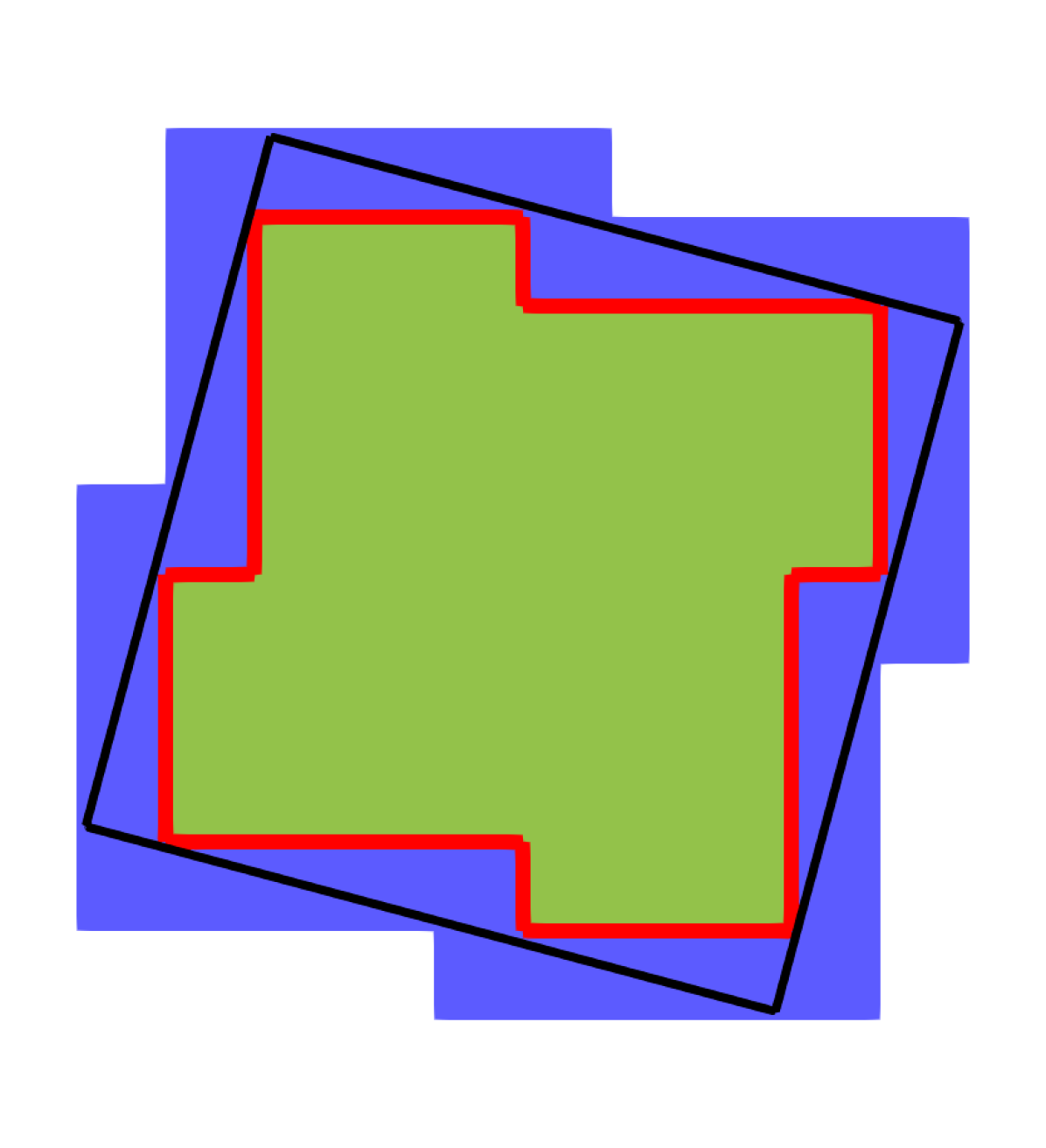
(a) $\lambda$ = 0

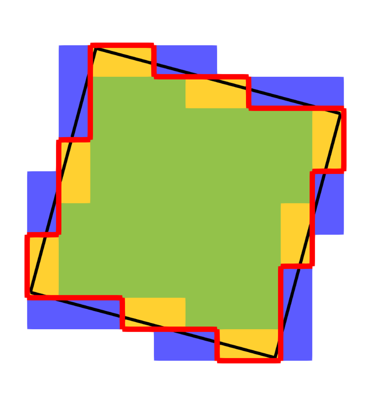
(b) $\lambda$ = 0.5

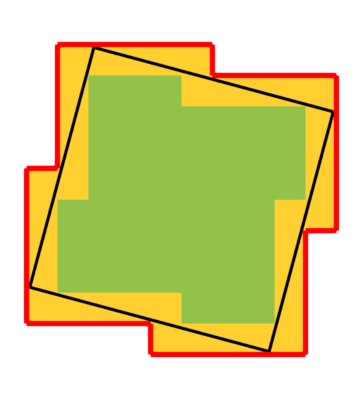
(c) $\lambda$ = 1

Figure 3: Surrogate boundary and the marker with varying $\lambda$: Figure showing the classification of a) Interior ($\blacksquare$); b) Intercepted ($\blacksquare$); c) FalseIntercepted ($\blacksquare$) with varying $\lambda$. Inactive elements do not form the incomplete octree and are not present. Note that (—) indicates the surrogate boundary whereas (—-) denotes the true boundary.

The surrogate domain $\tilde{\Omega}_{h}$ of size $h$ is defined as a set of elements with element size $||\Delta\boldsymbol{x}||\leq h$ such that when any extra element (of size $||\Delta\boldsymbol{x}||\leq h$) that belongs to the complement $\tilde{\Omega}_{h}^{c}$ of $\tilde{\Omega}_{h}$ is added, it must be classified as either Exterior or FalseIntercepted. A surrogate domain can be constructed as circumscribing ($\lambda=1$) or inscribing ($\lambda=0$) the true domain, or “something in between” ($\lambda\in(0,1)$) these two extreme cases. A surrogate boundary is the set of faces/edges that traverses the surrogate domain $\tilde{\Omega}_{h}$. Figure 3 illustrates a variety of surrogate domains and associated surrogate boundaries for a given geometry. We design algorithms such that the surrogate domain satisfies the following conditions to ensure correct computations:

• Watertightness: Ideally, the true boundary must be watertight or 2-manifold as nothing can enter or leave the domain. In practice, however, the SBM approach is robust to small gaps/overlaps.

• Single-cycle condition: The set of edges or faces that form the surrogate boundary must form one and exactly one cycle that traverses the surrogate domain $\tilde{\Omega}_{h}$. In other words, there should not be any self-intersections in the surrogate boundary.

In the next section, we describe the algorithms to construct the surrogate boundary for arbitrary choices of $\lambda$ in a massively parallel environment.

4 Algorithms and Implementation Details

4.1 Algorithms

To start the discussion of the algorithms for the efficient and accurate construction of surrogate domain and surrogate boundary for the SBM computations, we clarify some assumptions and motivations behind the choices described in what follows.

4.1.1 Assumptions regarding meshes

Before proceeding to the algorithm sections, we make the following assumption regarding the data structures.

1. No neighbor information: We assume that the mesh elements do not have access neighborhood information. Tagging neighbors is particularly challenging with unstructured meshes, as elements can have varying neighbors with no plausible upper limits.

2. Partitioned from get-go : The octree-based mesh data structure is partitioned right from the construction stage using distributed memory parallelism. This aspect has made octrees possible to scale to thousands of processors. This is in contrast to the traditional unstructured mesh generation, where the mesh is first generated on a single processor and later partitioned through a graph partitioning library such as ParMetis. This is an important aspect to consider while developing algorithms that retain the scalability of octree meshes.

3. Massively parallel environment: The algorithm proposed should scale to thousands of processors. We are not only interested in the accurate solution of PDEs but also in an efficient and scalable solution.

4. Different element sizes: Octrees can have different element sizes. We consider 2:1 balanced octrees during our algorithmic development [36]. Additionally, we assume that the Intercepted elements and Interior elements that are neighbors of the Intercepted elements (elements that share at least one node of the Intercepted elements) are at the same level. This is done to ensure that there are no hanging nodes, which retains the simplicity of algorithms without too much extra computational cost.

4.1.2 Algorithm for determining surrogate boundary for arbitrary boundary

With the above assumption in Section 4.1.1, we can define the algorithms for determining the surrogate boundary for any arbitrary choice of $\lambda$. The basic idea of the proposed algorithm is to rely on the connection between the elements through the nodes. We note that the nodes are shared across the elements in Continuous Galerkin (CG) Finite element method. Other researchers have leveraged this to implement several graph-based algorithms for unstructured meshes, even without any neighbor information stored in the mesh data structure [37]. This can be efficiently performed as a series of matvec operations—a key component in FEM libraries and can be performed in a highly efficient and scalable manner [34, 31, 38, 32].

Algorithm 1 SurrogateBoundaryIdentification: Identify the surrogate boundary

1:Incomplete octree mesh $\mathscr{O}$,Threshold factor $\lambda$

2:Surrogate boundary ($\tilde{\Gamma}$)

3:

4:Marker $\mathscr{M}_{1}\leftarrow$ GenerateMarkers($\mathscr{O},\lambda$) $\triangleright$ Algorithm 2.

5:Marker $\mathscr{M}_{2}$, FalseIntercepted Nodes $(\mathscr{N})\leftarrow$ GenerateNeighborsOfFalseIntercepted($\mathscr{O}$) $\triangleright$ Algorithm 3

6:Boundary $\tilde{\Gamma}$, Marker $M_{3}\leftarrow$ GetBoundary($\mathscr{O},\mathscr{M}_{2}$) $\triangleright$ Algorithm 4

7:return ($\tilde{{\Gamma}}$)

Algorithm 1 briefs the major step required to identify the surrogate boundary. We begin with identifying markers for each element (Algorithm 2). At this stage, each element is classified as Interior, Exterior, or Intercepted. Next, each Intercepted element is classified as FalseIntercepted depending on the value of $\lambda$. For accurate evaluation of the volume term within $\Omega$, we use $5^{dim}$ Gauss - Legendre points; i.e., each element is filled with 5 Gauss points in each dimension. This computational choice works well for all our results but can be easily changed at compile time.

Algorithm 2 GenerateMarkers: Generate Marker classification (Exterior, Interior, Intercepted, FalseIntercepted

1:Octree $\mathscr{O}$,Threshold factor $\lambda$

2:Marker $M$

3:

4:$\mathscr{M}\leftarrow[]$

5:for element $\in\mathscr{O}$  do $\triangleright$ Loop over the elements of octree

6:    count $\leftarrow$ 0

7:    for nodes $\in$ elements do $\triangleright$ Loop over the nodes of each element

8:        if nodes == Interior then $\triangleright$ Classify nodes as Exterior or Interior

9:           count++ $\triangleright$ Increment for Interior nodes of element             

10:    if count == num_nodes then

11:        $\mathscr{M}$[element] $\leftarrow$ Interior

12:    else if count == 0 then

13:        $\mathscr{M}$[element] $\leftarrow$ Exterior

14:    else

15:        $\mathscr{M}$[element] $\leftarrow$ Intercepted

16:        count_gp $\leftarrow$ 0 $\triangleright$ Counter for number of Gauss points that are Interior

17:        for gp $\in$ GaussPoints do

18:           if gp $\leftarrow$ Interior then

19:               count_gp ++            

20:           $\lambda_{c}\leftarrow$ count_gp/num_gp $\triangleright$ Fraction of Gauss point that are Interior

21:           if $\lambda_{c}\geq\lambda$ then $\triangleright$ Classify elements on the basis of the threshold $\lambda$

22:               $\mathscr{M}$[element] $\leftarrow$ FalseIntercepted                       

23:return ($\mathscr{M}$)

Algorithm 3 GenerateNeighborsOfFalseIntercepted: Generate neighbors of FalseIntercepted

1:Octree $\mathscr{O}$, Element marker $\mathscr{M}$

2:Marker $M$ with element marker for NeighborsFalseIntercepted, Nodal False Intercepted nodes $\mathscr{N}$

3:

4:$\mathscr{N}$_ghosted $\leftarrow$ [0] $\triangleright$ Vector of zeros with size of ghosted nodal vectors

5:for element $\in\mathscr{O}$ do

6:    if element == FalseIntercepted then

7:        for nodes $\in$ element do

8:           $\mathscr{N}$_ghosted[nodes] $\leftarrow$ 1 $\triangleright$ Assign value of 1 to all the nodes of the element tagged as FalseIntercepted             

9:$\mathscr{N}$ $\leftarrow$ GhostWrite($\mathscr{N}$_ghosted) $\triangleright$ Ghost write

10:$\mathscr{N}$_ghosted $\leftarrow$ GhostRead($\mathscr{N}$) $\triangleright$ Ghost read

11:for element $\in\mathscr{O}$ do

12:    if anyof(nodes) $\in$ element == 1 then $\triangleright$ If any of the nodes is marked as 1

13:        $\mathscr{M}$[element] $\leftarrow$ NeighborsFalseIntercepted    

14:return ($\mathscr{M}$,$\mathscr{N}$)

Removing FalseIntercepted elements from the domain requires a change of surrogate boundary. To identify the surrogate boundary, we generate the markers for neighbors of FalseIntercepted. Without the neighbor information within the mesh data structure, we rely on the efficient  matvec computation to achieve this task (Algorithm 3). This step can also be considered a scatter-to-gather transformation. Each FalseIntercepted element scatter the information by assigning the value of 1 to the incident nodes on that given element. In the second pass, each element gathers the data by looking into the values of the nodes that are incident on it. Once we have the nodal and elemental information about the NeighborsFalseIntercepted, we can compute the faces that form the new $\tilde{\Gamma}_{h}$. Two distinct cases exist:

1. If an element is marked as Intercepted, we proceed as usual. The face(s) of the element with all the nodes marked as Exterior is added to the surrogate boundary faces.

2. For the element marked NeighborsFalseIntercepted, we loop through the faces of the element. If all the nodes on a given face are either FalseIntercepted or Exterior, then and only then, they form the part of $\tilde{\Gamma}_{h}$.

Algorithm 4 GetBoundary: Get surrogate boundary

1:Octree $\mathscr{O}$, Element marker $\mathscr{M}$

2:Surrogate boundary $\tilde{\Gamma}$, Marker $\mathscr{M}$

3:

4:for element $\in\mathscr{O}$ do

5:    FaceBits $\leftarrow$ [false]

6:    for face $\in$ element do $\triangleright$ Loop over the faces of the element

7:        if $\mathscr{M}$[element] == Intercepted and allof(nodes $\in$ face == Exterior) then $\triangleright$ Condition for Interceptedelement

8:           FaceBits[face] $\leftarrow$ True

9:        else if $\mathscr{M}$[element] == NeighborsFalseIntercepted then $\triangleright$ Condition for NeighborsFalseInterceptedelements

10:           BoundaryFace $\leftarrow$ True

11:           for nodes $\in$ face do

12:               if (nodes == Exterior) or (nodes == FalseInterceptedNode) then $\triangleright$ Each node should be either Exterior or FalseIntercepted

13:                  continue

14:               else

15:                  BoundaryFace $\leftarrow$ False

16:                  break                                       

17:    if cycle(faceBits) then $\triangleright$ If opposite face of the same element forms the part of $\tilde{\Gamma}$

18:        $\mathscr{M}$[element] $\leftarrow$ FalseIntercepted

19:    else

20:        for face $\in$ element do $\triangleright$ Add faces to the surrogate domain $\tilde{\Gamma}$

21:           if faceBits[face] $\leftarrow$ true then

22:               $\tilde{\Gamma}\leftarrow$ $\tilde{\Gamma}$.push_back(face)                        

23:return ($\tilde{\Gamma}$,$\mathscr{M}$)

In some cases, we observe a cycle being formed where the opposite faces ($X_{i}^{-},X_{i}^{+},i=1\cdots$ dim) of a given element are both chosen to be part of the surrogate boundary. This violates the second condition of the surrogate boundary described in Section 3.1. We mark such elements as FalseIntercepted to resolve this issue. This ensures that only one of the sides $X_{i}^{-}$ or $X_{i}^{+}$ is selected to be part of the surrogate boundary depending on the side of NeighborsFalseIntercepted (Algorithm 4). Figure 3 shows the variation of the surrogate domain and surrogate boundary for different choices of $\lambda$. We note that all the steps in Algorithm 1 can be done efficiently in $\mathscr{O}(N)$ steps and require a small number of passes over the elements of the octree.

4.1.3 SBM computation

Once we set up the surrogate domain ($\tilde{\Omega}_{h}$) and resultant surrogate boundary ($\tilde{\Gamma}_{h}$) along with the associated markers, we proceed with the steps for the deployment of the SBM. Algorithm 5 briefs the major step for the SBM computation. We note that the elements marked as FalseIntercepted (and Exterior, if not using incomplete octree) are skipped over, whereas the volume integration is performed on other elements. Each face of the Intercepted and NeighborsFalseIntercepted element is checked to see if it belongs to the surrogate boundary $\tilde{\Gamma}_{h}$. If a given face belongs to $\tilde{\Gamma}_{h}$, the required surface integration (as given in Eq. 7) computation is performed and assembled to the global matrix and vector. Once the global matrix $\mathscr{A}$ and global vector $b$ are assembled, we solve the system of equations to obtain the solution $u^{h}$.

Algorithm 5 SBM: Shifted Boundary method

1:Octree $\mathscr{O}$, Element marker $\mathscr{M}$,Surrogate boundary $\tilde{\Gamma}$, PDE ($\mathscr{L}(u)=f$)

2:Solution of PDE: $u^{h}$

3:

4:for element $\in\mathscr{O}$ do

5:    if element == FalseIntercepted then

6:        continue

7:    else

8:        Assemble matrix ($\mathscr{A}$) and right hand side vector ($b$)

9:        if (element == Intercepted) or (element == NeighborsFalseIntercepted)  then

10:           for face $\in$ element do

11:               if face $\in\tilde{\Gamma}$ then

12:                  Assemble surface contribution to matrix ($\mathscr{A}$) and right hand side vector ($b$)                                       

13:Solve $\mathscr{A}u^{h}=b$ $\triangleright$ Solve system of linear equation

14:return $u^{h}$

4.2 Distance function calculation

Note that the SBM computations require evaluating the distance, $\boldsymbol{d}$, of Gauss points on the surrogate boundary to the closed point on the true boundary. This section focuses on calculating distance functions for intricate three-dimensional geometries. We consider the geometries to be represented in STL files, which are, in turn, represented by sets of triangles. SBM computation requires computing the distance function by finding the normal distance from the Gauss point to the nearest triangle. We store information about Gauss points and their corresponding distance functions to avoid repeated distance function calculations. This is particularly important for time-dependent problems on the static mesh as it prevents repetitive computation at the cost of extra memory.

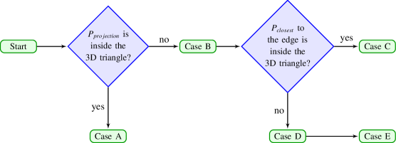
(a) Flowchart of distance calculation procedure.

(b) Case A:$P_{projection}$ falls inside the 3D triangle.

(c) Case B:$P_{projection}$ lies outside the 3D triangle.

(d) Case C:The shortest distance from the point to the triangle edges.

(e) Case D:The shortest distance from the point to the triangle edges, and the closest point ($P_{closest}$) fall outside of the triangle.

(f) Case E:The shortest distance from the point to the triangle vertexs.

Figure 4: Distance function calculation. As shown in the flowchart in (a), the projection of the point into the plane of the triangle can be inside or outside. If it falls outside, the point is projected to the three edges. If the closest of the edge projections is outside the triangle, then the closest point is computed to the vertices.

Algorithm 6 Overview: Calculation of distance functions

1:Gauss point positions on the surrogate boundary (GaussPoints), geometry, and mapping between Gauss points and distance functions

2:Distance function corresponding to each Gauss point

3:

4:for $P\in$ GaussPoints do

5:    if $P$ is already in the mapping then

6:        Use the precomputed distance function for $P$

7:    else

8:        Find the distance function from $P$ to the nearest triangle using NormalDistCalc $\triangleright$  Algorithm 7

9:        Save the mapping between $P$ and its distance function     

10:return distance functions for all Gauss points

Algorithm 7 NormalDistCalc: Calculation of normal distance to nearest triangle

1:k-d tree built from triangle centroids, Gauss point position ($P$), and geometry information

2:Distance function corresponding to the Gauss point

3:

4:Use the k-d tree to find the ID of the nearest triangle to the Gauss point $P$

5:Calculate the normal vector from $P$ to the nearest triangle by projecting the vector $\mathbf{PA}$ onto the triangle’s normal vector $\mathbf{n}$: $(\frac{\mathbf{PA}\cdot\mathbf{n}}{\lvert\mathbf{n}\rvert^{2}})\cdot\mathbf{n}$, where $A$ is one vertex position of the triangle

6:if the projection point is inside the 3D triangle then $\triangleright$  Algorithm 8

7:    Set the distance function as the normal vector to the nearest triangle

8:else

9:    Calculate the shortest distance from $P$ to the nearest triangle edge as the distance function $\triangleright$  Algorithm 9

10:return distance function

Algorithm 8 CheckInside3DTriangle: Check if point is inside 3D triangle

1:Projection point position ($P_{project}$) and vertex positions of triangle ($A$, $B$, $C$)

2:Whether the projection point is inside the 3D triangle

3:

4:Calculate cross products $\mathbf{u}=\mathbf{AB}\times\mathbf{AP_{project}},\mathbf{v}=\mathbf{BC}\times\mathbf{BP_{project}},\mathbf{w}=\mathbf{CA}\times\mathbf{CP_{project}}$

5:if $\mathbf{u}\cdot\mathbf{v}$ < 0 or $\mathbf{u}\cdot\mathbf{w}$ < 0 then

6:    return false

7:else

8:    return true

Algorithm 9 ShortestDist2TriEdge: Calculate the shortest distance to a triangle edge

1:Gauss point position $P$, and vertices of a triangle $A$, $B$, and $C$

2:Shortest distance vector from $P$ to a triangle edge

3:

4:Compute the projection of $P$ onto each triangle edge, i.e., $\mathbf{PP_{AB}}=\frac{\mathbf{AP}\cdot\mathbf{AB}}{{\lvert\mathbf{AB}\rvert}^{2}}\mathbf{AB}-\mathbf{AP}$, $\mathbf{PP_{BC}}=\frac{\mathbf{BP}\cdot\mathbf{BC}}{{\lvert\mathbf{BC}\rvert}^{2}}\mathbf{BC}-\mathbf{BP}$, $\mathbf{PP_{CA}}=\frac{\mathbf{CP}\cdot\mathbf{CA}}{{\lvert\mathbf{CA}\rvert}^{2}}\mathbf{CA}-\mathbf{CP}$, where $P_{AB}$, $P_{BC}$, $P_{CA}$ denote the closest points on edges $\overline{AB}$, $\overline{BC}$, $\overline{CA}$ to $P$

5:Compute the minimum distance from $P$ to each edge, i.e., $\lvert\mathbf{PP_{AB}}\rvert$, $\lvert\mathbf{PP_{BC}}\rvert$, $\lvert\mathbf{PP_{CA}}\rvert$ and find the closest point ($P_{closest}$) to $P$ within $P_{AB},P_{BC},P_{CA}$

6:if the $P_{closest}$ is inside the 3D triangle then $\triangleright$  Algorithm 8

7:    Set the distance function as the $\mathbf{PP_{closest}}$

8:else

9:    Calculate the shortest distance function from $P$ to the nearest triangle vertex, $\mathbf{PP_{vertex}}$

10:return distance function

The procedure for calculating the distance function is outlined in Algorithm 6 and Figure 4(a). We utilize the algorithm presented in Algorithm 7 to compute the normal distance between Gauss points and the nearest triangle, as depicted in Figure 4(b). We leverage a k-d tree to efficiently search the closest triangle using nanoflann library [39] to expedite this process. Specifically, the k-d tree is constructed from the triangle centroids, and during the Gauss point iteration, the k-d tree assists in identifying the nearest triangle and obtaining its ID for each Gauss point. Nonetheless, in certain instances, the projection points from Gauss points to triangles may fall outside the triangle, as illustrated in Figure 4(c). To handle such situations, we have incorporated two additional procedures. Firstly, Algorithm 8 verifies whether the projection points lie within the nearest triangle. Secondly, Algorithm 9 determines the shortest distance between the point and the edges of the triangle, as shown in Figure 4(d). It is worth noting that the projection method we use to find the closest point on the triangle edges to the Gauss point may not always result in a point inside the triangle in three dimensions, as shown in Figure 4(e). In such cases, we search for the closest vertex of the triangle and calculate the distance function based on it, as illustrated in Figure 4(f) and Algorithm 9.

5 Numerical results

This section presents numerical results for the simulation of Poisson equation and the equations of linear elasticity, over domains of complex geometry. We note the following important points for the readers to interpret the results:

• The integration for the weak form is performed using standard $(p+1)^{dim}$ Gauss quadrature points in all the elements, where $p$ is the order of the polynomial finite element interpolation basis. We use the linear basis function ($p=1$) in all reported results.

• We report accuracy by comparing the numerical solution against analytical solutions. This post-processing operation to compute the $L^{2}$-error is performed on each element using five Gauss points per dimension. The reported $L^{2}$-error is computed as

  $$||e||_{L^{2}(\Omega)}=||u^{h}-u_{exact}||_{L^{2}(\Omega)}=\sqrt{\int_{\Omega}(u^{h}-u_{exact})^{2}d\Omega}\;.$$

  Note that the error is computed on the true domain $\Omega$. In particular, the SBM solution is smoothly extended over elements that intersect $\Omega$ but are not part of the SBM active domain $\tilde{\Omega}_{h}$.

• In order to compare errors from different simulations, for which the sizes of the domains $\Omega$ may differ, we report the normalized error, defined as:

  $$L_{2N}(\Omega)=\frac{||e||_{L^{2}(\Omega)}}{\sqrt{\int_{\Omega}d\Omega}}\;.$$

• We define the improvement factor $I_{2\lambda}$ (Eq. • ‣ 5) as the metric for comparison between different surrogates with respect to the case in which $\lambda=1$. We recall that $\lambda=1$ corresponds to the case in which $\tilde{\Omega}_{h}\supset\Omega$, that is $\tilde{\Omega}_{h}$ circumscribes $\Omega$. When comparing simulations performed with different values of $\lambda$, a lower value of $I_{2\lambda}$, corresponds to better solutions:

  $$I_{2\lambda}=\frac{L_{2N}(\Omega;\lambda)}{L_{2N}(\Omega;\lambda=1)}\;.$$

• We recall the definition of $\lambda,(0\leq\lambda\leq 1)$ as the elemental volume fraction of the domain $\Omega$ . More specifically, $\lambda$ is a threshold used to check whether an Intercepted element needs also to be classified as FalseIntercepted element.

5.1 Identifying the optimal surrogate boundary

Recall that our goal is to construct the optimal surrogate boundary that minimizes the distance $\boldsymbol{d}$, the distance between $\Gamma$ and $\tilde{\Gamma}_{h}$. Our approach yields that $\lambda=0.5$ minimizes $\boldsymbol{d}$. We illustrate this result using a canonical test example. Consider a rotated rectangle inclined at a 15^∘ angle with respect to the background octree mesh. We compute the distance (Eq. 18, the RMS distance) between the surrogate boundary and true boundary for a range of surrogate boundary choices by varying $\lambda\in[0,1]$.

Figure 5 compares the value of RMS distance for different $\lambda$, for different mesh resolutions (identified by the level of refinement). Observe that $\lambda=0.5$ yields the minimal RMS distance, irrespective of the level of the mesh resolution. In addition to conducting tests at a 15^∘ angle, we also carried out experiments at 10^∘, 20^∘, 30^∘, and 40^∘ angles, paired with varying mesh refinement levels. The results consistently pointed towards $\lambda=0.5$ as the value that assures the least RMS distance. Figure 6 further demonstrates these conclusions for various geometries defined by rotating a square at various angles. Thus, choosing $\lambda=0.5$ provides a simple and effective strategy for constructing the surrogate boundary. In the subsequent sections, we analyze improvement in solution accuracy resulting from constructing an optimal surrogate boundary ($\lambda=0.5$) as compared to a non-optimal surrogate (usually $\lambda=0,\lambda=1$).

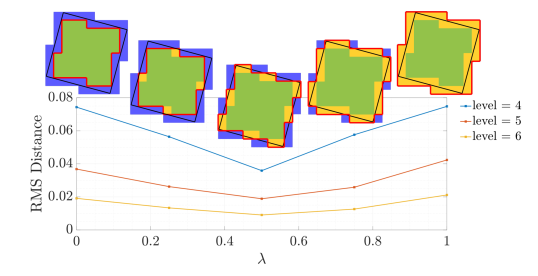
Figure 5: Constructing the surrogate boundary for a rotated square on a Cartesian mesh. The figure shows the RMS distance with varying $\lambda$ values for different octree levels. In each inset, the solid red line represents the surrogate surface, while the solid black line represents the true boundary. FalseIntercepted elements are marked by $\blacksquare$, whereas TrueIntercepted elements are marked by $\blacksquare$ and Interior elements by $\blacksquare$.

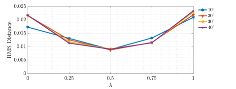
Figure 6: RMS of the distance between the true and surrogate boundaries, for a square rotated by various angles ($10^{\circ}$, $20^{\circ}$, $30^{\circ}$, $40^{\circ}$), and grid refinement level equal to 6.

5.2 Solving Poisson’s equation on disk

We next utilize the optimal surrogate construction approach to solve Poisson’s equation when $\Omega$ has a simple shape: a circular disk. This is an exact geometry, and several ways exist to construct an axis-aligned surrogate boundary for a circle. Consider a disk with a radius $R=0.5$, centered at ($x_{0}=0.5,y_{0}=0.5$). We solve Poisson’s equation on this geometry with a Dirichlet boundary of $u_{0}=0.01$ on the boundary and forcing term $f=1$. We choose the penalty parameter $\alpha$ to be 400. This problem has an analytical solution given by: $u(r)=0.25(R^{2}-r^{2})+u_{0}$, where $r$ is the distance from the center ($r=\sqrt{(x-x_{0})^{2}+(y-y_{0})^{2}}$).

(a) Normalized $L_{2}$ error convergence

(b) Improvement factors, $I_{2\lambda}$. (The lower the better)

Figure 7: Left: Mesh convergence plot solving the Poisson’s equation on a disk. Each line represents a convergence plot with a specific surrogate boundary constructed using a $\lambda$. Notice that while all surrogate choices exhibit the expected slope, the $\lambda=0.5$ surrogate produces the lowest error for any mesh size. Right: The improvement plot shows that the optimal surrogate produces more accurate solutions.

Figure 7 shows the mesh convergence plot for different choices of $\lambda$. We observe second-order convergence in normalized error $L_{2N}$ (Figure 7(a)), irrespective of the choice of $\lambda$. However, the optimal choice of $\lambda$, and thereby of surrogate boundary, can significantly reduce the magnitude of the error. We observe that choosing $\lambda=0.5$ yields minimal error that is almost an order of magnitude lower when compared to the previously reported surrogate boundary choices of $\lambda=0$ [22] or $\lambda=1$ [31]. Figure 7(b) compares this improvement factor for the cases of $\lambda=0.0$ and $\lambda=0.5$ with respect to case of $\lambda=1$ (note that $I_{2\lambda}=1$ for $\lambda=1$). The choice $\lambda=0.5$ produces errors at least three times lower than the case $\lambda=0$ or $\lambda=1$ across all mesh resolutions. This improvement is significant, considering that the computational effort in identifying the optimal surrogate is minimal.

5.3 Complex geometries

We next showcase the ability of the SBM to accurately solve the Poisson’s equation over three-dimensional objects. We consider three standard benchmarks exhibiting complex geometries and sharp corners: the Stanford Bunny, the Moai, and the Armadillo. For all three-dimensional cases, the penalty parameter $\alpha$ is set to 400. We use the method of manufactured solutions to construct an analytical solution against which to compare the SBM results. This allows rigorous comparison across different values of $\lambda$. The analytical solution for each of the cases is given as:

$$u(x,y,z)=\left\{\begin{aligned} &\cos(\pi x)\,y\,\sin(\pi z),&\mathrm{\;Stanford\;bunny;}\\ &(1-x)\,(1-y)\,\cos(3\pi z),&\mathrm{\;Moai;}\\ &\cos(\pi x)\,(1-y)\,\sin(\pi z),&\mathrm{\;Armadillo.}\end{aligned}\right.$$ (21)

For each object, we perform a mesh convergence analysis by solving the Poisson’s equation using the optimal surrogate ($\lambda=0.5$) and compare the accuracy against the choice of surrogates with $\lambda=1$ and $\lambda=0$. Figure 8 compares $I_{2\lambda}$ for various values of $\lambda$ and different mesh sizes. We can see that the value of $\lambda=0.5$ consistently outperforms $\lambda=0$ and $\lambda=1$ in terms of accuracy. This demonstrates both the importance of choosing an optimal $\lambda$ as well as the robustness of the proposed algorithm for solving PDEs on complex geometries.

Stanford Bunny
Moai
Armadillo

Figure 8: Solving Poisson’s equations on complex 3D domains using the optimized surrogate boundary.

Next, to test the algorithm’s robustness, we explore its performance on a geometry exhibiting an extremely complex topology. We consider a simulation on a three-dimensional model of the Eiffel Tower, in STL format. Figure 9(a) shows the surface representation of the geometry, with a very large number of small holes and sharp corners. We choose a manufactured solution of the form:

$$u(x,y,z)=(1-x)(1-y)\cos(3\pi z).$$ (22)

Figure 9(b) shows the resulting solution field. Finally, we notice the same trend in $L^{2}$-error, with surrogates defined by $\lambda=0.5$ outperforming the other choices (Figure 9(c)).

(a) STL file

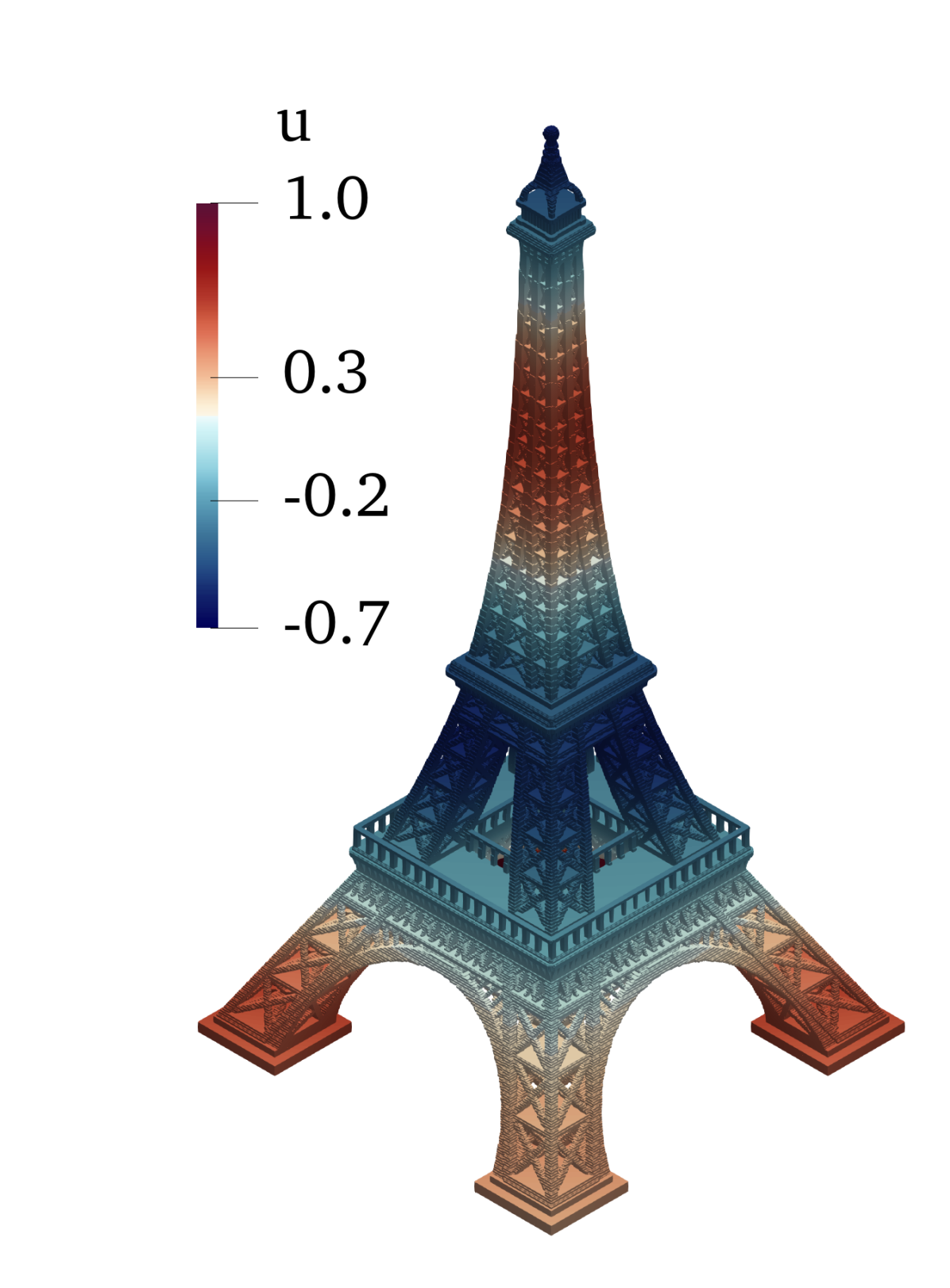
(b) Solution contour

(c) Error in the $L_{2}$-norm

Figure 9: Solving Poisson’s equation on the Eiffel tower model using SBM:(a) The STL file of the Eiffel tower immersed into the background mesh and the bounding box. (b) Solution contour of Eiffel Tower with mesh size equal to $1/2^{10}$. (c) Improvement plot of $I_{2\lambda}$ and the results show that the optimal surrogate boundary can reduce the $L_{2N}$ error.

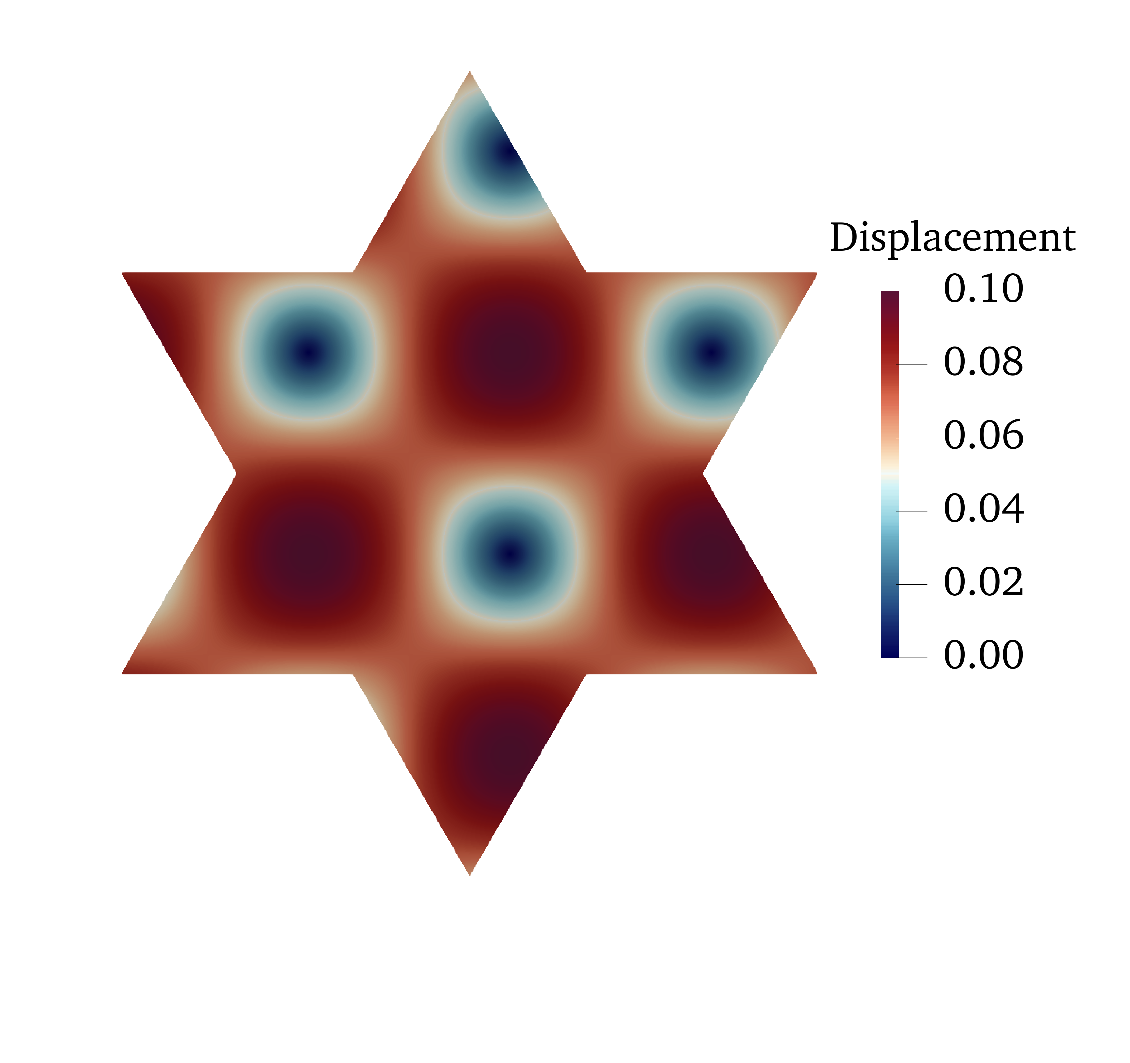
(a) Displacement solution contour

(b) Normalized $L_{2}$ error convergence

(c) Improvement in $L_{2}$ error in $u_{x}$

(d) Improvement in $L_{2}$ error in $u_{y}$

Figure 10: Solving linear elasticity on a star shape using SBM: Figure 10(a) shows the contour for the displacement magnitude contour for $h=2.4/2^{10}$. Figure 10(b) shows the convergence plot of $L_{2N}$ error for $u_{x}$ and $u_{y}$ for different choices of $\lambda$. Figure 10(c) and Figure 10(d) shows the improvement in $L_{2N}$ error when using the optimal surrogate, $\lambda=0.5$, for $u_{x}$ and $u_{y}$.

5.4 Linear elasticity

Our final example showcases the SBM approach for solving linear elasticity equations. As shown in Figure 10(a), we consider a star-shaped domain. The sharp corners and non-convex geometry makes this a challenging case. We set Young’s modulus $E$ to be 1 and Poisson’s ratio $\nu$ to be 0.3. The elastic tensor $\boldsymbol{C}$ is for plain stress. The penalty parameter $\gamma$ is equal to 400. We consider a manufactured solution of the form:

$$\left\{\begin{aligned} u_{x}(x,y)=\frac{\sin(\pi x)\cos(\pi y)}{10}\\ u_{y}(x,y)=\frac{\cos(\pi x)\sin(\pi y)}{10}\end{aligned}_{\textstyle\raisebox{2.0pt}{.}}\quad\right.$$ (23)

Figure 10(a) shows the displacement solution contour, while Figure 10(b) shows the convergence of $L_{2N}$ error. Similar to Poisson’s case, we observe a second-order convergence in $L^{2}$-error. We see a significant improvement in $L^{2}$-error by choosing a value of $\lambda=0.5$ when compared to $\lambda=0$ or $\lambda=1$ both for the x-displacement, $u_{x}$ (Figure 10(c)) and y-displacement, $u_{y}$(Figure 10(d)). This improved performance is seen across all mesh refinements.

(a) Total solve time with increase in the number of processors.

(b) Percentage of time for individual steps.

Figure 11: Scaling behavior and percentage of time at different stages of the SBM computation in 2D on TACC  Stampede2.

5.5 Parallel computing scaling

(a) Total solve time with increase in the number of processors.

(b) Percentage of time for individual steps.

Figure 12: Scaling behavior and percentage of time at different stages of the SBM computation for 3D Stanford Bunny on TACC  Stampede2.

Finally, we present some scaling results of our framework on TACC Stampede2 SKX and  ICX nodes. To perform the scaling test, we consider the problem described in Section 5.2. We choose $\lambda$ of 0.5 for the scaling test as it conforms to the optimal surrogate. The strong scaling test considers octree at a level of 10 ($h=1/2^{10}$). Figure 11(a) shows the variation of total solve time with increasing the number of processors.; with a near-ideal scaling behavior. Figure 11(b) shows the percentage of time taken by the different stages. We observe that the extra step for constructing the surrogate amounts to almost 10% of the total time. We note that this step, along with octree construction, needs to be performed only once for a static mesh and will be amortized to a smaller fraction for transient problems. As expected, we observe that the overall runtime is dominated by linear algebra solve.

In addition to the 2D case, we conducted a scaling study on a three-dimensional Stanford Bunny, as presented in Section 5.5. For the strong scaling test, we utilized an octree level of 9 ($h=1/2^{9}$). The total solving time with respect to the number of processors is shown in Figure 12(a), while Figure 12(b) illustrates the percentage of time taken by each stage. Unlike the 2D case, the incomplete octree construction time became the problem’s bottleneck. However, the octree construction procedure is a one-time event if we encounter time-dependent problems. Notably, the matrix assembly time is similar to the vector assembly time for this three-dimensional case, given that we calculate and store distance function information during vector assembly and reuse it during matrix assembly to minimize the distance function calculation time. Furthermore, we implemented k-D tree to improve the time required to calculate the distance function in three-dimensional complex shapes. Thus, our algorithms and implementation ensure good scalability, making this approach a practical strategy for solving PDEs in complex domains using conceptually simple octree meshes.

6 Conclusions and Future Work

By shifting the enforcement of boundary conditions from the actual boundary to a surrogate boundary, the SBM allows for the use of Cartesian meshes, eliminating the need for laborious and time-consuming body-fitted meshes around complex geometries. In this work, we answer some key questions regarding the scalable and accurate deployment of the Shifted Boundary Method. The key findings of this work are as follows: (a) identification of an optimal surrogate boundary parameter that greatly reduces numerical error in the SBM, (b) rigorous theoretical analysis demonstrating the optimal convergence of SBM on extended surrogate domains, (c) successful deployment of the SBM on massively parallel octree meshes, including handling of incomplete octrees, and (d) successful application of the SBM to various simulations involving complex shapes, including those with sharp corners and different topologies, with a focus on Poisson’s equation and linear elasticity equations. This work sets the stage for a massively parallel, octree-based, general-purpose solution framework—using the SBM—for solving PDEs on arbitrarily complex geometries.

There are several avenues for future developments. One avenue we are actively exploring involves extending the SBM on the octree framework to multi-physics and coupled PDEs, including Navier-Stokes, Cahn-Hilliard Navier-Stokes, and the Possion-Nernst-Planck equations. Another avenue is to extend the framework to account for moving boundaries, with a natural extension to efficiently model fluid-structure interaction problems across complex geometries. Another active avenue of research is to develop robust preconditioners and architecture-aware solvers (for example, GPU-accelerated multigrid methods) for such SBM on octree approaches. A final straightforward extension is to explore the utility of higher-order basis functions and their tradeoff on error vs. time-to-solve.

Appendix A Proof of Proposition 1

Proposition. There exists an extension $\bar{u}$ of $u$ in $\Omega_{\mathrm{ext}}$, such that:

1. $-\Delta\bar{u}=\bar{f}$ in $\Omega_{\mathrm{ext}}$; and

2. if $u\in H^{2}(\Omega)$, then $\bar{u}\in H^{2}(\tilde{\Omega}_{h})$, with $\|\bar{u}\|_{H^{2}(\tilde{\Omega}_{h})}\leq C\;\|u\|_{H^{2}(\Omega)}$.

Proof

To fulfill a) and b) above, let $\Omega_{\Delta}=\Omega_{\mathrm{ext}}\setminus\mathrm{cl}(\Omega)$, where $\mathrm{cl}(\Omega)$ is the closure of $\Omega$. The boundary $\partial\Omega_{\Delta}$ of the set $\Omega_{\Delta}$ is decomposed as the union of two disjoint boundaries, namely $\partial\Omega_{\Delta}=\Gamma_{0}\cup\Gamma_{1}$, with $\Gamma_{0}=\partial\Omega$ and $\Gamma_{1}=\partial\Omega_{\mathrm{ext}}$. Then we define

$$\bar{u}\;=\;\begin{cases}u\quad\mbox{in }\mathrm{cl}(\Omega)\;,\\ \hat{u}\quad\mbox{in }\Omega_{\Delta}\;,\end{cases}$$ (24)

where $\hat{u}$ is the solution of

$$\begin{cases}-\Delta\hat{u}=\bar{f}\quad\mbox{in }\Omega_{\Delta}\;,\\ \quad\,\,\hat{u}=u_{D}\quad\mbox{on }\Gamma_{0}\;,\\ \quad\,\,\hat{u}=\varphi\quad\mbox{on }\Gamma_{1}\;,\end{cases}$$ (25)

and $\varphi$ is chosen so that

$$\frac{\partial\hat{u}}{\partial n}=\frac{\partial u}{\partial n}\quad\mbox{on }\Gamma_{0}\;,\\$$ (26)

with $\partial(\cdot)/\partial n$ the normal derivative along $\boldsymbol{n}$ (i.e.  along the unit normal to $\Gamma_{0}$ pointing outside of $\Omega$). To motivate Eq. 26, observe that $\Gamma_{0}$ and $\Gamma_{1}$ are smooth curves and that $u_{D}\in H^{3/2}(\Gamma_{0})$. Since $f\in L^{2}(\Omega)$, then, by the regularity theorem of elliptic problems, we have $u\in H^{2}(\Omega)$ and consequently $\displaystyle\frac{\partial u}{\partial n}\in H^{1/2}(\Gamma_{0})$. Similarly, if $\varphi\in H^{3/2}(\Gamma_{1})$, then from $\bar{f}\in L^{2}(\Omega_{\Delta})$ and $u_{D}\in H^{3/2}(\Gamma_{0})$ we deduce $\hat{u}\in H^{2}(\Omega_{\Delta})$ and consequently $\displaystyle\frac{\partial\hat{u}}{\partial n}\in H^{1/2}(\Gamma_{0})$. In order to deduce $\bar{u}\in H^{2}(\Omega_{\mathrm{ext}})$, we need to have

$$u_{|\Gamma_{0}}=\hat{u}_{|\Gamma_{0}}\;,$$

which is true since $u_{|\Gamma_{0}}=\hat{u}_{|\Gamma_{0}}=u_{D}$ on $\Gamma_{0}$, and

$$\nabla u_{|\Gamma_{0}}=\nabla\hat{u}_{|\Gamma_{0}}\;.$$

This last condition can be decomposed into the matching of the component of the gradient normal to $\Gamma_{0}$, which is precisely Eq. 26, and the matching of the component of the gradient tangent to $\Gamma_{0}$, namely

$$\frac{\partial\hat{u}}{\partial\tau}=\frac{\partial\hat{u}}{\partial\tau}\quad\mbox{on }\Gamma_{0}\;,\\$$ (27)

which is true since they both coincide with $\displaystyle\frac{\partial u_{D}}{\partial\tau}$ on $\Gamma_{0}$.

Next, we verify the existence of $\varphi$ in Eq. 25 such that Eq. 26 is verified. The solution of Eq. 25 is equivalent to the solution of the two sub-problems

$$\begin{cases}-\Delta\hat{u}_{1}=\bar{f}\quad\ \ \mbox{in }\Omega_{\Delta}\;,\\ \quad\,\,\hat{u}_{1}=u_{D}\quad\mbox{on }\Gamma_{0}\;,\\ \quad\,\,\hat{u}_{1}=0\quad\ \ \mbox{on }\Gamma_{1}\;,\end{cases}\;\,$$ (28a)

$$\begin{cases}-\Delta\hat{u}_{0}=0\quad\mbox{in }\Omega_{\Delta}\;,\\ \quad\,\,\hat{u}_{0}=0\quad\mbox{on }\Gamma_{0}\;,\\ \quad\,\,\hat{u}_{0}=\varphi\quad\mbox{on }\Gamma_{1}\;,\end{cases}$$ (28b)

when we set $\hat{u}=\hat{u}_{1}+\hat{u}_{0}$, so that condition Eq. 26 becomes

$$\frac{\partial\hat{u}_{0}}{\partial n}=\frac{\partial u}{\partial n}-\frac{\partial\hat{u}_{1}}{\partial n}\;\in H^{1/2}(\Gamma_{0})\;.$$ (29)

Let us then introduce the the operator

$$\mathscr{T}:H^{1/2}(\Gamma_{1}) \rightarrow\;H^{-1/2}(\Gamma_{0})$$

$$\varphi \mapsto\;\left.\frac{\partial\hat{u}_{0}}{\partial n}\right|_{\Gamma_{0}}$$

and check that $\mathscr{T}$ is onto (i.e., surjective), namely that $\mathrm{Im}(\mathscr{T})=\left\{\mathscr{T}\varphi:\varphi\in H^{1/2}(\Gamma_{1})\right\}$ coincides with $H^{-1/2}(\Gamma_{0})$. We argue by contradiction: since $\mathrm{Im}(\mathscr{T})$ is a closed subspace of $H^{-1/2}(\Gamma_{0})$, assume that its orthogonal space contains elements $\eta\neq 0$. Any such $\eta\in H^{-1/2}(\Gamma_{0})$ then satisfies

$$(\eta,\mathscr{T}\varphi)_{H^{-1/2}(\Gamma_{0})}=0\;,\qquad\forall\varphi\in H^{-1/2}(\Gamma_{0})\;.$$

Note that the inner product in $H^{-1/2}(\Gamma_{0})$ is the duality pairing

$${}_{H^{-1/2}(\Gamma_{0})}\langle\mathscr{T}\varphi\;,\,R\eta\rangle_{H^{1/2}(\Gamma_{0})}\;,$$

where $R\eta=z_{|\Gamma_{1}}$ with $z$ the solution of the problem

$$\begin{cases}\;\;-\Delta z=0\quad\mbox{in }\Omega_{\Delta}\;,\\ \;\;\quad\,\,z=0\quad\mbox{on }\Gamma_{1}\;,\\[2.84544pt] \;\;\;\;\displaystyle\frac{\partial z}{\partial n}=\eta\quad\mbox{on }\Gamma_{0}\;.\end{cases}$$ (30)

Hence, for any $\varphi\in H^{1/2}(\Gamma_{1})$, we have

$$0 =\;_{H^{-1/2}(\Gamma_{0})}\langle\frac{\partial\hat{u}_{0}}{\partial n}\;,\,z\rangle_{H^{1/2}(\Gamma_{0})}$$

$$=\;_{H^{-1/2}(\Gamma_{0})}\langle\frac{\partial\hat{u}_{0}}{\partial n}\;,\,z\rangle_{H^{1/2}(\Gamma_{0})}\;+\;\underbrace{{}_{H^{-1/2}(\Gamma_{1})}\langle\frac{\partial\hat{u}_{0}}{\partial n}\;,\,z\rangle_{H^{1/2}(\Gamma_{1})}}_{\mbox{$=0$ by~{}\hyperref@@ii[eq:z]{Eq.~{}\ref*{eq:z}}}}$$

$$=\;_{H^{-1/2}(\partial\Omega_{\Delta})}\langle\frac{\partial\hat{u}_{0}}{\partial n}\;,\,z\rangle_{H^{1/2}(\partial\Omega_{\Delta})}$$

$$=\;\int_{\Omega_{\Delta}}\underbrace{\Delta\hat{u}_{0}}_{\mbox{$=0$ by~{}\hyperref@@ii[eq:ext_u1_sub0]{Eq.~{}\ref*{eq:ext_u1_sub0}}}}\,z\;+\;\int_{\Omega_{\Delta}}\nabla\hat{u}_{0}\cdot\nabla z\qquad\qquad\qquad\qquad\ \ \ \ \mbox{(using integration by parts)}$$

$$=\;\int_{\Omega_{\Delta}}\nabla\hat{u}_{0}\cdot\nabla z$$

$$=\;\int_{\Omega_{\Delta}}\underbrace{\Delta z}_{\mbox{$=0$ by~{}\hyperref@@ii[eq:z]{Eq.~{}\ref*{eq:z}}}}\,\hat{u}_{0}\;+\;_{H^{-1/2}(\partial\Omega_{\Delta})}\langle\frac{\partial z}{\partial n}\;,\,\hat{u}_{0}\rangle_{H^{1/2}(\partial\Omega_{\Delta})}\qquad\qquad\mbox{(using integration by parts)}$$

$$=\;\underbrace{{}_{H^{-1/2}(\Gamma_{0})}\langle\frac{\partial z}{\partial n}\;,\,\hat{u}_{0}\rangle_{H^{1/2}(\Gamma_{0})}}_{\mbox{$=0$ by~{}\hyperref@@ii[eq:ext_u1_sub0]{Eq.~{}\ref*{eq:ext_u1_sub0}}}}\;+\;_{H^{-1/2}(\Gamma_{1})}\langle\frac{\partial z}{\partial n}\;,\,\hat{u}_{0}\rangle_{H^{1/2}(\Gamma_{1})}$$

$$=\;_{H^{-1/2}(\Gamma_{1})}\langle\eta\;,\,\varphi\rangle_{H^{1/2}(\Gamma_{1})}\;.$$ (31)

We conclude then that $\eta$ is the null linear form on $H^{1/2}(\Gamma_{0})$, that is $\eta=0$. As a consequence of $\mathscr{T}$ being onto, picking

$$\eta\;=\;\frac{\partial u}{\partial n}-\frac{\partial\hat{u}_{1}}{\partial n}\;,$$

there exists $\phi\in H^{1/2}(\Gamma_{1})$ such that the solution of Eq. 28b satisfies

$$\frac{\partial\hat{u}_{0}}{\partial n}=\eta\;.$$

In addition, since $\eta\in H^{1/2}(\Gamma_{0})$, we get $\hat{u}_{0}\in H^{2}(\Omega_{\Delta})$ and $\varphi=(\hat{u}_{0})_{|\Gamma_{1}}\in H^{3/2}(\Gamma_{1})$, whence $\hat{u}\in H^{2}(\Omega_{\Delta})$ as desired. $\Box$

References

- Mittal and Iaccarino [2005] R. Mittal, G. Iaccarino, Immersed boundary methods, Annual Review of Fluid Mechanics 37 (2005) 239–261.
- Peskin [1972] C. S. Peskin, Flow patterns around heart valves: a numerical method, Journal of Computational Physics 10 (1972) 252–271.
- Xu et al. [2016] F. Xu, D. Schillinger, D. Kamensky, V. Varduhn, C. Wang, M.-C. Hsu, The tetrahedral finite cell method for fluids: Immersogeometric analysis of turbulent flow around complex geometries, Computers & Fluids 141 (2016) 135–154.
- Hoang et al. [2019] T. Hoang, C. V. Verhoosel, C.-Z. Qin, F. Auricchio, A. Reali, E. H. van Brummelen, Skeleton-stabilized immersogeometric analysis for incompressible viscous flow problems, Computer Methods in Applied Mechanics and Engineering 344 (2019) 421–450.
- de Prenter et al. [2019] F. de Prenter, C. Verhoosel, E. van Brummelen, Preconditioning immersed isogeometric finite element methods with application to flow problems, Computer Methods in Applied Mechanics and Engineering 348 (2019) 604–631.
- Zhu et al. [2019] Q. Zhu, F. Xu, S. Xu, M.-C. Hsu, J. Yan, An immersogeometric formulation for free-surface flows with application to marine engineering problems, Computer Methods in Applied Mechanics and Engineering 361 (2019) 112748.
- Saurabh et al. [2021] K. Saurabh, B. Gao, M. Fernando, S. Xu, M. A. Khanwale, B. Khara, M.-C. Hsu, A. Krishnamurthy, H. Sundar, B. Ganapathysubramanian, Industrial scale large eddy simulations with adaptive octree meshes using immersogeometric analysis, Computers & Mathematics with Applications 97 (2021) 28–44.
- Hsu et al. [2016] M.-C. Hsu, C. Wang, F. Xu, A. J. Herrema, A. Krishnamurthy, Direct immersogeometric fluid flow analysis using B-rep CAD models, Computer Aided Geometric Design 43 (2016) 143–158.
- Wang et al. [2017] C. Wang, F. Xu, M.-C. Hsu, A. Krishnamurthy, Rapid b-rep model preprocessing for immersogeometric analysis using analytic surfaces, Computer aided geometric design 52 (2017) 190–204.
- Balu et al. [2023] A. Balu, M. R. Rajanna, J. Khristy, F. Xu, A. Krishnamurthy, M.-C. Hsu, Direct immersogeometric fluid flow and heat transfer analysis of objects represented by point clouds, Computer Methods in Applied Mechanics and Engineering 404 (2023) 115742.
- Xu et al. [2021] F. Xu, E. L. Johnson, C. Wang, A. Jafari, C.-H. Yang, M. S. Sacks, A. Krishnamurthy, M.-C. Hsu, Computational investigation of left ventricular hemodynamics following bioprosthetic aortic and mitral valve replacement, Mechanics Research Communications 112 (2021) 103604.
- Parvizian et al. [2007] J. Parvizian, A. Düster, E. Rank, Finite cell method: h- and p- extension for embedded domain methods in solid mechanics, Computational Mechanics 41 (2007) 122–133.
- Massing et al. [2015] A. Massing, M. Larson, A. Logg, M. Rognes, A Nitsche-based cut finite element method for a fluid-structure interaction problem, Communications in Applied Mathematics and Computational Science 10 (2015) 97–120.
- Burman et al. [2015] E. Burman, S. Claus, P. Hansbo, M. G. Larson, A. Massing, CutFEM: Discretizing geometry and partial differential equations, Int. J. Numer. Methods Eng. 104 (2015) 472–501.
- Burman [2010] E. Burman, Ghost penalty, C. R. Math. 348 (2010) 1217–1220.
- Burman and Hansbo [2014] E. Burman, P. Hansbo, Fictitious domain methods using cut elements: Iii. a stabilized Nitsche method for Stokes’ problem, ESAIM: Mathematical Modelling and Numerical Analysis 48 (2014) 859–874.
- Schott et al. [2015] B. Schott, U. Rasthofer, V. Gravemeier, W. Wall, A face-oriented stabilized Nitsche-type extended variational multiscale method for incompressible two-phase flow, Int. J. Numer. Methods Eng. 104 (2015) 721–748.
- Schott and Wall [2014] B. Schott, W. Wall, A new face-oriented stabilized xfem approach for 2d and 3d incompressible navier–Stokes equations, Comput. Methods Appl. Mech. Eng. 276 (2014) 233–265.
- Burman and Hansbo [2012] E. Burman, P. Hansbo, Fictitious domain finite element methods using cut elements: II. A stabilized Nitsche method, Applied Numerical Mathematics 62 (2012) 328–341.
- Burman and Fernández [2014] E. Burman, M. A. Fernández, An unfitted Nitsche method for incompressible fluid–structure interaction using overlapping meshes, Comput. Methods Appl. Mech. Eng. 279 (2014) 497–514.
- Saurabh et al. [2022] K. Saurabh, M. Ishii, M. A. Khanwale, H. Sundar, B. Ganapathysubramanian, Scalable adaptive algorithms for next-generation multiphase simulations, arXiv preprint arXiv:2209.12130 (2022).
- Main and Scovazzi [2018a] A. Main, G. Scovazzi, The shifted boundary method for embedded domain computations. part i: Poisson and stokes problems, Journal of Computational Physics 372 (2018a) 972–995.
- Main and Scovazzi [2018b] A. Main, G. Scovazzi, The shifted boundary method for embedded domain computations. part ii: Linear advection-diffusion and incompressible navier-stokes equations, J. Comput. Phys. 372 (2018b) 996–1026.
- Karatzas et al. [2020] E. N. Karatzas, G. Stabile, L. Nouveau, G. Scovazzi, G. Rozza, A reduced-order shifted boundary method for parametrized incompressible navier-stokes equations, Computer Methods in Applied Mechanics and Engineering 370 (2020) 113273.
- Atallah et al. [2020] N. M. Atallah, C. Canuto, G. Scovazzi, The second-generation shifted boundary method and its numerical analysis, Computer Methods in Applied Mechanics and Engineering 372 (2020) 113341.
- Atallah et al. [2021a] N. Atallah, C. Canuto, G. Scovazzi, The shifted boundary method for solid mechanics, International Journal for Numerical Methods in Engineering 122 (2021a) 5935–5970.
- Atallah et al. [2021b] N. Atallah, C. Canuto, G. Scovazzi, Analysis of the Shifted Boundary Method for the Poisson problem in domains with corners, Mathematics of Computation 90 (2021b) 2041–2069.
- Colomés et al. [2021] O. Colomés, A. Main, L. Nouveau, G. Scovazzi, A weighted shifted boundary method for free surface flow problems, Journal of Computational Physics 424 (2021) 109837.
- Atallah et al. [2022] N. M. Atallah, C. Canuto, G. Scovazzi, The high-order shifted boundary method and its analysis, Computer Methods in Applied Mechanics and Engineering 394 (2022) 114885.
- Zeng et al. [2022] X. Zeng, G. Stabile, E. N. Karatzas, G. Scovazzi, G. Rozza, Embedded domain reduced basis models for the shallow water hyperbolic equations with the shifted boundary method, Computer Methods in Applied Mechanics and Engineering 398 (2022) 115143.
- Saurabh et al. [2021] K. Saurabh, M. Ishii, M. Fernando, B. Gao, K. Tan, M.-C. Hsu, A. Krishnamurthy, H. Sundar, B. Ganapathysubramanian, Scalable adaptive pde solvers in arbitrary domains, in: Proceedings of the International Conference for High Performance Computing, Networking, Storage and Analysis, 2021, pp. 1–15.
- Burstedde et al. [2011] C. Burstedde, L. C. Wilcox, O. Ghattas, p4est: Scalable algorithms for parallel adaptive mesh refinement on forests of octrees, SIAM Journal on Scientific Computing 33 (2011) 1103–1133.
- Sundar et al. [2008] H. Sundar, R. S. Sampath, G. Biros, Bottom-up construction and 2: 1 balance refinement of linear octrees in parallel, SIAM Journal on Scientific Computing 30 (2008) 2675–2708.
- Ishii et al. [2019] M. Ishii, M. Fernando, K. Saurabh, B. Khara, B. Ganapathysubramanian, H. Sundar, Solving PDEs in space-time: 4D tree-based adaptivity, mesh-free and matrix-free approaches, in: Proceedings of the International Conference for High Performance Computing, Networking, Storage and Analysis, 2019, pp. 1–61.
- Alzetta et al. [2018] G. Alzetta, D. Arndt, W. Bangerth, V. Boddu, B. Brands, D. Davydov, R. Gassmoeller, T. Heister, L. Heltai, K. Kormann, M. Kronbichler, M. Maier, J.-P. Pelteret, B. Turcksin, D. Wells, The deal.II library, version 9.0, Journal of Numerical Mathematics 26 (2018) 173–183.
- Sundar et al. [2008] H. Sundar, R. Sampath, G. Biros, Bottom-up construction and 2:1 balance refinement of linear octrees in parallel, SIAM Journal on Scientific Computing 30 (2008) 2675–2708. doi:10.1137/070681727.
- Bogle et al. [2019] I. Bogle, K. Devine, M. Perego, S. Rajamanickam, G. M. Slota, A parallel graph algorithm for detecting mesh singularities in distributed memory ice sheet simulations, in: Proceedings of the 48th International Conference on Parallel Processing, 2019, pp. 1–10.
- Fernando et al. [2017] M. Fernando, D. Duplyakin, H. Sundar, Machine and application aware partitioning for adaptive mesh refinement applications, in: Proceedings of the 26th International Symposium on High-Performance Parallel and Distributed Computing, 2017, pp. 231–242.
- Blanco and Rai [2014] J. L. Blanco, P. K. Rai, nanoflann: a C++ header-only fork of FLANN, a library for nearest neighbor (NN) with kd-trees, https://github.com/jlblancoc/nanoflann, 2014.