Beyond Conservatism: Diffusion Policies in
Offline Multi-agent Reinforcement Learning

Abstract

We present a novel Diffusion Offline Multi-agent Model (DOM2) for offline Multi-Agent Reinforcement Learning (MARL). Different from existing algorithms that rely mainly on conservatism in policy design, DOM2 enhances policy expressiveness and diversity based on diffusion. Specifically, we incorporate a diffusion model into the policy network and propose a trajectory-based data-augmentation scheme in training. These key ingredients make our algorithm more robust to environment changes and achieve significant improvements in performance, generalization and data-efficiency. Our extensive experimental results demonstrate that DOM2 outperforms existing state-of-the-art methods in multi-agent particle and multi-agent MuJoCo environments, and generalizes significantly better in shifted environments thanks to its high expressiveness and diversity. Furthermore, DOM2 shows superior data efficiency and can achieve state-of-the-art performance with $20+$ times less data compared to existing algorithms.

1 Introduction

Offline reinforcement learning (RL), commonly referred to as batch RL, aims to learn efficient policies exclusively from previously gathered data without interacting with the environment Lange et al. (2012); Levine et al. (2020). Since the agent has to sample the data from a fixed dataset, naive offline RL approaches fail to learn policies for out-of-distribution actions or states Wu et al. (2019); Kumar et al. (2019), and the obtained Q-value estimation for these actions will be inaccurate with unpredictable consequences. Recent progress in tackling the problem focuses on conservatism by introducing regularization terms in the training of actors and critics Fujimoto et al. (2019); Kumar et al. (2020a); Fujimoto and Gu (2021); Kostrikov et al. (2021a); Lee et al. (2022). Conservatism-based offline RL algorithms have also achieved significant progress in difficult offline multi-agent reinforcement learning settings (MARL) Jiang and Lu (2021); Yang et al. (2021); Pan et al. (2022).

Despite the potential benefits, existing methods have limitations in several aspects. Firstly, the design of the policy network and the corresponding regularizer limits the expressiveness and diversity due to conservatism. Consequently, the resulting policy may be suboptimal and difficult to represent complex strategies Kumar et al. (2019); Wang et al. (2022). Secondly, in multi-agent scenarios, the conservatism-based method is prone to getting trapped in poor local optima. This occurs when each agent is incentivized to maximize its own reward without efficient cooperation with other agents in existing algorithms Yang et al. (2021); Pan et al. (2022).

To demonstrate this phenomenon, we conduct experiment on a simple MARL scenario consisting of $3$ agents and $6$ landmarks (Fig. 1a), to highlight the importance of policy expressiveness and diversity in MARL. In this scenario, the agents are asked to cover $3$ landmarks and are rewarded based on their proximity to the nearest landmark while being penalized for collisions. We first train the agents with $6$ target landmarks and then randomly dismiss $3$ of them in evaluation. Our experiments demonstrate that existing methods (MA-CQL and OMAR detailed in Section 3.2 Pan et al. (2022)), which constrain policies through regularization, limit the expressiveness of each agent and hinder the ability of the agents to cooperate with diversity. As a result, only limited solutions are found. Therefore, in order to design robust algorithms with good generalization capabilities, it is crucial to develop methods beyond conservatism for better performance and more efficient cooperation among agents.

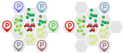
(a)

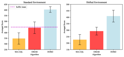
(b)

Figure 1: 1a: Standard environment (left) and shifted environment dismissing 3 landmarks randomly (right). 1b: Results in different environments. For experimental details, see Appendix B.3.

To boost the policy expressiveness and diversity, we propose a novel algorithm based on diffusion for the offline multi-agent setting, called Diffusion Offline Multi-Agent Model (DOM2). Diffusion model has shown significant success in generating data with high quality and diversity Ho et al. (2020); Song et al. (2020a); Croitoru et al. (2023) and our goal is to leverage this advantage to promote expressiveness and diversity in policy learning of RL. Specifically, the policy for each agent is built using the accelerated DPM-solver to sample actions Lu et al. (2022). In order to train an appropriate policy that performs well, we propose a trajectory-based data-augmentation method to facilitate policy training by efficient data sampling. These techniques enable the policy to generate solutions with high quality and diversity and overcome the limitations of conservatism-based approaches. In the $3$-agent example, we show that DOM2 can find a more diverse set of solutions with high performance and generalization (Fig. 1b), compared to conservatism-based methods such as MA-CQL and OMAR Pan et al. (2022). Our contributions are summarized as follows.

• We propose a novel Diffusion Offline Multi-Agent Model (DOM2) algorithm to address the limitations of conservatism-based methods. DOM2 consists of three critical components: diffusion-based policy with an accelerated solver, appropriate policy regularizer, and a trajectory-based data augmentation method for enhancing learning.

• We conduct extensive numerical experiments on Multi-agent Particles Environments (MPE) and Multi-agent MuJoCo HalfCheetah environments. Our results show that DOM2 achieves significantly better performance improvement over state-of-the-art methods.

• We show that our diffusion-based method DOM2 possesses much better generalization abilities and outperforms existing methods in shifted environments (trained in standard environments). Moreover, DOM2 is ultra-data-efficient, and achieves SOTA performance with $20\text{+}$ times less data.

2 Related Work

Offline RL and MARL: Distribution shift is a key obstacle in offline RL and multiple methods have been proposed to tackle the problem based on conservatism to constrain the policy or Q-value by regularizers Wu et al. (2019); Kumar et al. (2019); Fujimoto et al. (2019); Kumar et al. (2020a). Policy regularization ensures the policy to be close to the behavior policy via a policy regularizer, e.g., BRAC Wu et al. (2019), BEAR Kumar et al. (2019), BCQ Fujimoto et al. (2019), TD3+BC Fujimoto and Gu (2021), implicit update Peng et al. (2019); Siegel et al. (2020); Nair et al. (2020) and importance sampling Kostrikov et al. (2021a); Swaminathan and Joachims (2015); Liu et al. (2019); Nachum et al. (2019). Critic regularization instead constrains the Q-values for stability, e.g., CQL Kumar et al. (2020a), IQL Kostrikov et al. (2021b), and TD3-CVAE Rezaeifar et al. (2022). On the other hand, Multi-Agent Reinforcement Learning (MARL) has made significant process under the centralized training with decentralized execution (CTDE) paradigm Oliehoek et al. (2008); Matignon et al. (2012), such as MADDPG Lowe et al. (2017), MATD3 Ackermann et al. (2019), IPPO de Witt et al. (2020), MAPPO Yu et al. (2021), VDN Sunehag et al. (2017) and QMIX Rashid et al. (2018) in decentralized critic and centralized critic setting. The offline MARL problem has also attracted attention and conservatism-based methods have been developed, e.g., MA-BCQ Jiang and Lu (2021), MA-ICQ Yang et al. (2021), MA-CQL and OMAR Pan et al. (2022).

Diffusion Models: Diffusion model Ho et al. (2020); Song et al. (2020a); Sohl-Dickstein et al. (2015); Song and Ermon (2019); Song et al. (2020b), a specific type of generative model, has shown significant success in various applications, especially in generating images from text descriptions Nichol et al. (2021); Ramesh et al. (2022); Saharia et al. (2022). Recent works have focused on the foundation of diffusion models, e.g., the statistical theory Chen et al. (2023), and the accelerating method for sampling Lu et al. (2022); Bao et al. (2022). Generative model has been applied to policy modeling, including conditional VAE Kingma and Welling (2013), diffusers Janner et al. (2022); Ajay et al. (2022) and diffusion-based policy Wang et al. (2022); Chen et al. (2022); Lu et al. (2023) in the single-agent setting. Our method successfully introduces the diffusion model with the accelerated solver to offline multi-agent settings.

3 Background

In this section, we introduce the offline multi-agent reinforcement learning problem and provide preliminaries for the diffusion probabilistic model as the background for our proposed algorithm.

Offline Multi-Agent Reinforcement Learning. A fully cooperative multi-agent task can be modeled as a decentralized partially observable Markov decision process (Dec-POMDP) Oliehoek and Amato (2016) with $n$ agents consisting of a tuple $G=\langle\mathcal{I},\mathcal{S},\mathcal{O},\mathcal{A},\Pi,\mathcal{P},\mathcal{R},n,\gamma\rangle$. Here $\mathcal{I}$ is the set of agents, $\mathcal{S}$ is the global state space, $\mathcal{O}=(\mathcal{O}_{1},...,\mathcal{O}_{n})$ is the set of observations with $\mathcal{O}_{n}$ being the set of observation for agent $n$. $\mathcal{A}=(\mathcal{A}_{1},...,\mathcal{A}_{n})$ is the set of actions for the agents ($\mathcal{A}_{n}$ is the set of actions for agent $n$), $\Pi=(\Pi_{1},...,\Pi_{n})$ is the set of policies, and $\mathcal{P}$ is the function class of the transition probability $\mathcal{S}\times\mathcal{A}\times\mathcal{S}^{\prime}\rightarrow[0,1]$. At each time step $t$, each agent chooses an action $a_{j}^{t}\in\mathcal{A}_{j}$ based on the policy $\pi_{j}\in\Pi_{j}$ and historical observation $o_{j}^{t-1}\in\mathcal{O}_{j}$. The next state is determined by the transition probability $P\in\mathcal{P}$. Each agent then receives a reward $r_{j}^{t}\in\mathcal{R}:\mathcal{S}\times\mathcal{A}\rightarrow\mathbb{R}$ and a private observation $o_{j}^{t}\in\mathcal{O}_{i}$. The goal of the agents is to find the optimal policies $\bm{\pi}=(\pi_{1},...,\pi_{n})$ such that each agent can maximize the discounted return: $\mathbb{E}[\sum_{t=0}^{\infty}\gamma^{t}r_{j}^{t}]$ (the joint discounted return is $\mathbb{E}[\sum_{j=1}^{n}\sum_{t=0}^{\infty}\gamma^{t}r_{j}^{t}]$), where $\gamma$ is the discount factor. Offline reinforcement learning requires that the data to train the agents is sampled from a given dataset $\mathcal{D}$ generated from some potentially unknown behavior policy $\bm{\pi}_{\bm{\beta}}$ (which can be arbitrary). This means that the procedure for training agents is separated from the interaction with environments.

Conservative Q-Learning. For training the critic in offline RL, the conservative Q-Learning (CQL) method Kumar et al. (2020a) is to train the Q-value function $Q_{{\bm{\phi}}}(\bm{o},\bm{a})$ parameterized by $\bm{\phi}$, by minimizing the temporal difference (TD) loss plus the conservative regularizer. Specifically, the objective to optimize the Q-value for each agent $j$ is given by:

$$\mathcal{L}(\bm{\phi}_{j}) =\mathbb{E}_{(\bm{o}_{j},\bm{a}_{j})\sim\mathcal{D}_{j}}[(Q_{\bm{\phi}_{j}}(\bm{o}_{j},\bm{a}_{j})-y_{j})^{2}]$$ (1)

$$+\zeta\mathbb{E}_{(\bm{o}_{j},\bm{a}_{j})\sim\mathcal{D}_{j}}[\log\sum_{\tilde{\bm{a}}_{j}}\exp(Q_{\bm{\phi}_{j}}(\bm{o}_{j},\tilde{\bm{a}}_{j}))-Q_{\bm{\phi}_{j}}(\bm{o}_{j},\bm{a}_{j})].$$

The first term is the TD error to minimize the Bellman operator with the double Q-learning trick Fujimoto et al. (2019); Hasselt (2010); Lillicrap et al. (2015), where $y_{j}=r_{j}+\gamma\min_{k=1,2}\overline{Q}_{\bm{\phi}_{j}}^{k}(\bm{o}^{\prime}_{j},\overline{\pi}_{j}(\bm{o}^{\prime}_{j}))$, $\overline{Q}_{\bm{\phi}_{j}},\overline{\pi}_{j}$ denotes the target network and $\bm{o}^{\prime}_{j}$ is the next observation for agent $j$ after taking action $\bm{a}_{j}$. The second term is a conservative regularizer, where $\tilde{\bm{a}}_{j}$ is a random action uniformly sampled in the action space and $\zeta$ is a hyperparameter to balance two terms. The regularizer is to address the extrapolation error by encouraging large Q-values for state-action pairs in the dataset and penalizing low Q-values of state-action pairs.

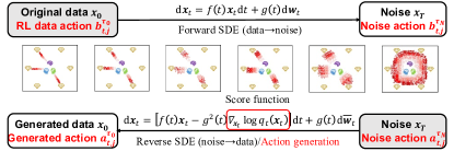
Figure 2: Diffusion probabilistic model as a continuous-time stochastic differential equation (SDE) Song et al. (2020a) and relationship with Offline MARL.

Diffusion Probabilistic Model. We present a high-level introduction to the Diffusion Probabilistic Model (DPM) Sohl-Dickstein et al. (2015); Song et al. (2020a); Ho et al. (2020) (detailed introduction is in Appendix A). DPM is a deep generative model that learns the unknown data distribution $\bm{x}_{0}\sim q_{0}(\bm{x}_{0})$ from the dataset. The process of data generation is modeled by a predefined forward noising process characterized by a stochastic differential equation (SDE) ${\rm{d}}\bm{x}_{t}=f(t)\bm{x}_{t}{\rm{d}}t+g(t){\rm{d}}\bm{w}_{t}$ (Eq. (5) in Song et al. (2020a)) and a trainable reverse denoising process characterized by the SDE ${\rm{d}}\bm{x}_{t}=[f(t)\bm{x}_{t}-g^{2}(t)\nabla_{\bm{x}_{t}}\log q_{t}(\bm{x}_{t})]{\rm{d}}t+g(t){\rm{d}}\overline{\bm{w}}_{t}$ (Eq. (6) in Song et al. (2020a)) shown in Fig. 2. Here $\bm{w}_{t},\overline{\bm{w}}_{t}$ are standard Brownian motions, $f(t),g(t)$ are pre-defined functions such that $q_{0t}(\bm{x}_{t}|\bm{x}_{0})=\mathcal{N}(\bm{x}_{t};\alpha_{t}\bm{x}_{0},\sigma^{2}_{t}\bm{I})$ for some constant $\alpha_{t},\sigma_{t}>0$ and $q_{T}(\bm{x}_{T})\approx\mathcal{N}(\bm{x}_{T};\bm{0},\tilde{{\sigma}}^{2}\bm{I})$ is almost a Gaussian distribution for constant $\tilde{{\sigma}}>0$. However, there exists an unknown term $-\sigma_{t}\nabla_{\bm{x}_{t}}\log q_{t}(\bm{x}_{t})$, which is called the score function. In order to generate data close to the distribution $q_{0}(\bm{x}_{0})$ by the reverse SDE, DPM defines a score-based model $\bm{\epsilon}_{\bm{\theta}}(\bm{x}_{t},t)$ to learn the score function and optimize parameter $\bm{\theta}$ such that $\bm{\theta}^{*}={\arg\min}_{\bm{\theta}}\mathbb{E}_{\bm{x}_{0}\sim q_{0}(\bm{x}_{0}),\bm{\epsilon}\sim\mathcal{N}(\bm{0},\bm{I}),t\sim\mathcal{U}(0,T)}[\|\epsilon-\bm{\epsilon}_{\bm{\theta}}(\alpha_{t}\bm{x}_{0}+\sigma_{t}\bm{\epsilon},t)\|^{2}_{2}]$ ($\mathcal{U}(0,T)$ is the uniform distribution in $[0,T]$, same later). With the learned score function, we can sample data by discretizing the reverse SDE. To enable faster sampling, DPM-solver Lu et al. (2022) provides an efficiently faster sampling method and the first-order iterative equation (Eq. (3.7) in Lu et al. (2022)) to denoise is given by $\bm{x}_{t_{i}}=\frac{\alpha_{t_{i}}}{\alpha_{t_{i-1}}}\bm{x}_{t_{i-1}}-\sigma_{t_{i}}(\frac{\alpha_{t_{i}}\sigma_{t_{i-1}}}{\alpha_{t_{i-1}}\sigma_{t_{i}}}-1)\bm{\epsilon}_{\bm{\theta}}(\bm{x}_{t_{i-1}},t_{i-1})$.

In Fig. 2, we highlight a crucial message that we can efficiently incorporate the procedure of data generation into offline MARL as the action generator. Intuitively, we can utilize the fixed dataset to learn an action generator by noising the sampled actions in the dataset, and then denoising it inversely. The procedure assembles data generation in the diffusion model. However, it is important to note that there is a critical difference between the objectives of diffusion and RL. Specifically, in diffusion, the goal is to generate data with a distribution close to the distribution of the training dataset, whereas in offline MARL, one hopes to find actions (policies) that maximize the joint discounted return. This difference influences the design of the action generator. Properly handling it is the key in our design, which will be detailed below in Section 4.

4 Proposed Method

In this section, we present the DOM2 algorithm, which is shown in Fig. 3. In the following, we first discuss how we generate the actions with diffusion in Section 4.1. Next, we show how to design appropriate objective functions in policy learning in Section 4.2. We then present the data augmentation method in Section 4.3. Finally, we present the whole procedure of DOM2 in Section 4.4.

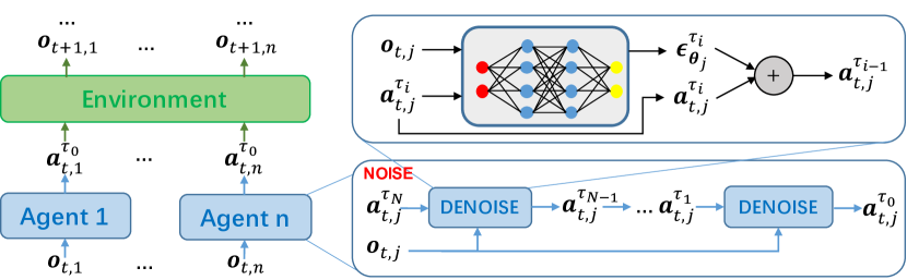
Figure 3: Diagram of the DOM2 algorithm. Each agent generates actions with diffusion.

4.1 Diffusion in Offline MARL

We first present the diffusion component in DOM2, which generates actions by denoising a Gaussian noise iteratively (shown on the right side of Fig. 3). Denote the timestep indices in an episode by $\{t\}_{t=1}^{T}$, the diffusion step indices by $\tau\in[\tau_{0},\tau_{N}]$, and the agent by $\{j\}_{j=1}^{n}$. Below, to facilitate understanding, we introduce the diffusion idea in continuous time, based on Song et al. (2020a); Lu et al. (2022). We then present our algorithm design by specifying the discrete DPM-solver-based steps Lu et al. (2022) and discretized diffusion timestep, i.e., from $[\tau_{0},\tau_{N}]$ to $\{\tau_{i}\}_{i=0}^{N}$.

(Noising) Noising the action in diffusion is modeled as a forward process from $\tau_{0}$ to $\tau_{N}$. Specifically, we start with the collected action data at $\tau_{0}$, denoted by $\bm{b}_{t,j}^{\tau_{0}}\sim\bm{\pi}_{\bm{\beta}_{j}}(\cdot|\bm{o}_{t,j})$, which is collected from the behavior policy $\bm{\pi}_{\bm{\beta}_{j}}(\cdot|\bm{o}_{t,j})$. We then perform a set of noising operations on intermediate data $\{\bm{b}_{t,j}^{\tau}\}_{\tau\in[\tau_{0},\tau_{N}]}$, and eventually generate $\bm{b}_{t,j}^{\tau_{N}}$, which (ideally) is close to Gaussian noise at $\tau_{N}$.

This forward process satisfies that for $\forall\tau\in[\tau_{0},\tau_{N}]$, the transition probability $q_{\tau_{0}\tau}(\bm{b}_{t,j}^{\tau}|\bm{b}_{t,j}^{\tau_{0}})=\mathcal{N}(\bm{b}_{t,j}^{\tau};\alpha_{\tau}\bm{b}_{t,j}^{\tau_{0}},\sigma_{\tau}^{2}\bm{I})$ Lu et al. (2022). The selection of the noise schedules $\alpha_{\tau},\sigma_{\tau}$ enables that $q_{\tau_{N}}(\bm{b}_{t,j}^{\tau_{N}}|\bm{o}_{t,j})\approx\mathcal{N}(\bm{b}_{t,j}^{\tau_{N}};\bm{0},\tilde{\sigma}^{2}\bm{I})$ for some $\tilde{\sigma}>0$, which is almost a Gaussian noise. According to Song et al. (2020a); Kingma et al. (2021), there exists a corresponding reverse process of SDE from $\tau_{N}$ to $\tau_{0}$, which is based on Eq. (2.4) in Lu et al. (2022) and takes into consideration the conditioning on $\bm{o}_{t,j}$:

$${\rm{d}}\bm{a}^{\tau}_{t,j}=[f(\tau)\bm{a}^{\tau}_{t,j}-g^{2}(\tau)\underbrace{\nabla_{\bm{b}^{\tau}_{t,j}}q_{\tau}(\bm{b}^{\tau}_{t,j}|\bm{o}_{t,j})}_{\text{Neural Network }\bm{\epsilon}_{\bm{\theta}_{j}}}]{\rm{d}}\tau+g(\tau){\rm{d}}\overline{\bm{w}}_{\tau},\bm{a}^{\tau_{N}}_{t,j}\sim q_{\tau_{N}}(\bm{b}_{t,j}^{\tau_{N}}|\bm{o}_{t,j}),$$ (2)

where $f(\tau)=\frac{{\rm{d}}\log\alpha_{\tau}}{{\rm{d}}\tau},g^{2}(\tau)=\frac{{\rm{d}}\sigma_{\tau}^{2}}{{\rm{d}}\tau}-2\frac{{\rm{d}}\log\alpha_{\tau}}{{\rm{d}}\tau}\sigma_{\tau}^{2}$ and $\overline{\bm{w}}_{t}$ is a standard Brownion motion, and $\bm{a}^{\tau_{0}}_{t,j}$ is the generated action for agent $j$ at time $t$.

To fully determine the reverse process of SDE described by Eq. (2), we need the access to the conditional score function $-\sigma_{\tau}\nabla_{\bm{b}^{\tau}_{t,j}}q_{\tau}(\bm{b}^{\tau}_{t,j}|\bm{o}_{t,j})$ at each $\tau$. We use a neural network $\bm{\epsilon}_{\bm{\theta}_{j}}(\bm{b}_{t,j}^{\tau},\bm{o}_{t,j},\tau)$ to represent it and the architecture is the multiple-layered residual network, which is called U-Net Ho et al. (2020) shown in Fig. 8. The objective of optimizing the parameter $\bm{\theta}_{j}$ is Lu et al. (2022):

$$\mathcal{L}_{bc}({\bm{\theta}_{j}})=\mathbb{E}_{(\bm{o}_{t,j},\bm{a}_{t,j}^{\tau_{0}})\sim\mathcal{D}_{j},\bm{\epsilon}\sim\mathcal{N}(\bm{0},\bm{I}),\tau\in\mathcal{U}(\{\tau_{i}\}_{i=0}^{N})}[\|\bm{\epsilon}-\bm{\epsilon}_{\bm{\theta}_{j}}(\alpha_{\tau}\bm{a}_{t,j}^{\tau_{0}}+\sigma_{\tau}\bm{\epsilon},\bm{o}_{t,j},\tau)\|_{2}^{2}].$$ (3)

(Denoising) After training the neural network $\bm{\epsilon}_{\bm{\theta}_{j}}$, we can then generate the actions by solving the diffusion SDE Eq. (2) (plugging in $-\bm{\epsilon}_{\bm{\theta}_{j}}(\bm{a}_{t,j}^{\tau},\bm{o}_{t,j},\tau)/\sigma_{\tau}$ to replace the true score function $\nabla_{\bm{b}_{t,j}^{\tau}}\log q_{\tau}(\bm{b_{t,j}^{\tau}}|\bm{o}_{t,j})$). Here we evolve the reverse process of SDE from $\bm{a}^{\tau_{N}}_{t,j}\sim\mathcal{N}(\bm{a}_{t,j}^{\tau_{N}};\bm{0},\bm{I})$, a Gaussian noise, and we take $\bm{a}^{\tau_{0}}_{t,j}$ as the final action. In our algorithm, to facilitate faster sampling, we discretize the reverse process of SDE in $[\tau_{0},\tau_{N}]$ into $N+1$ diffusion timesteps $\{\tau_{i}\}_{i=0}^{N}$ (the partition details are shown in Appendix A) and adopt the first-order DPM-solver-based method (Eq. (3.7) in Lu et al. (2022)) to iteratively denoise from $\bm{a}^{\tau_{N}}_{t,j}\sim\mathcal{N}(\bm{a}_{t,j}^{\tau_{N}};\bm{0},\bm{I})$ to $\bm{a}^{\tau_{0}}_{t,j}$ for $i=N,...,1$ written as:

$$\bm{a}_{t,j}^{\tau_{i-1}}=\frac{\alpha_{\tau_{i-1}}}{\alpha_{\tau_{i}}}\bm{a}_{t,j}^{\tau_{i}}-\sigma_{\tau_{i}}\left(\frac{\alpha_{\tau_{i}}\sigma_{\tau_{i-1}}}{\alpha_{\tau_{i-1}}\sigma_{\tau_{i}}}-1\right)\bm{\epsilon}_{\bm{\theta}_{j}}(\bm{a}_{t,j}^{\tau_{i}},\bm{o}_{t,j},\tau_{i})\text{ for }i=N,...1,$$ (4)

and such iterative denoising steps are corresponding to the diagram in the right side of Fig. 3.

4.2 Policy Improvement

Notice that only optimizing $\bm{\theta}_{j}$ by Eq. (3) is not sufficient in offline MARL, because then the generated actions will only be close to the behavior policy under diffusion. To achieve policy improvement, we follow Wang et al. (2022) to take the Q-value into consideration and use the following loss function:

$$\mathcal{L}({\bm{\theta}}_{j})=\mathcal{L}_{bc}({\bm{\theta}_{j}})+\mathcal{L}_{q}({\bm{\theta}}_{j})=\mathcal{L}_{bc}({\bm{\theta}_{j}})-\tilde{\eta}\mathbb{E}_{(\bm{o}_{j},\bm{a}_{j})\sim\mathcal{D}_{j},\bm{a}_{j}^{\tau_{0}}\sim\pi_{\bm{\theta}_{j}}}[Q_{{\bm{\phi}}_{j}}(\bm{o}_{j},\bm{a}_{j}^{\tau_{0}})].$$ (5)

The second term $\mathcal{L}_{q}({\bm{\theta}_{j}})$ is called Q-loss Wang et al. (2022) for policy improvement , where $\bm{a}_{j}^{\tau_{0}}$ is generated by Eq. (4), ${\bm{\phi}}_{j}$ is the network parameter of Q-value function for agent $j$, $\tilde{\eta}=\frac{\eta}{\mathbb{E}_{(\bm{s}_{j},\bm{a}_{j})\sim\mathcal{D}}[Q_{{\bm{\phi}}_{j}}(\bm{o}_{j},\bm{a}_{j})]}$ and $\eta$ is a hyperparameter. This Q-value is normalized to control the scale of Q-value functions Fujimoto and Gu (2021) and $\eta$ is used to balance the weights. The combination of two terms ensures that the policy can preferentially sample actions with high values. The reason is that the policy trained by optimizing Eq. (5) can generate actions with different distributions compared to the behavior policy, and the policy prefers to sample actions with higher Q-values (corresponding to better performance). To train efficient Q-values for policy improvement, we optimize Eq. (1) as the objective Kumar et al. (2020a).

4.3 Data Augmentation

Algorithm 1 Data $\mathtt{Augmentation}$

1:  Input: Dataset $\mathcal{D}$ with trajectories $\{\mathcal{T}_{i}\}_{i=1}^{L}$.

2:  $\mathcal{D}^{\prime}\leftarrow\mathcal{D}$

3:  for every $r_{\text{th}}\in\mathcal{R}$ do

4:     $\mathcal{D}^{\prime}\leftarrow\mathcal{D}^{\prime}+\{\mathcal{T}_{i}\in\mathcal{D}|Return(\mathcal{T}_{i})\geq r_{\text{th}}\}$.

5:  end for

6:  Return: Augmented dataset $\mathcal{D}^{\prime}$.

In DOM2, in addition to the design of the novel policy with their training objectives, we also introduce a data-augmentation method to scale up the size of the dataset (shown in Algorithm 1). Specifically, we replicate trajectories $\mathcal{T}_{i}\in\mathcal{D}$ with high return values (i.e., with the return value, denoted by $Return(\mathcal{T}_{i})$, higher than threshold values) in the dataset. Specifically, we define a set of threshold values $\mathcal{R}=\{r_{\text{th},1},...,r_{\text{th},K}\}$. Then, we compare the reward of each trajectory with every threshold value and replicate the trajectory once whenever its return is higher than the compared threshold (Line 4), such that trajectories with higher returns can replicate more times. Doing so allows us to create more data efficiently and improve the performance of the policy by increasing the probability of sampling trajectories with better performance in the dataset.

4.4 The DOM2 Algorithm

The resulting DOM2 algorithm is presented in Algorithm 2. Line 1 is the initialization step. Line 2 is the data-augmentation step. Line 5 is the sampling procedure for the preparation of the mini-batch data from the augmented dataset to train the agents. Lines 6 and 7 are the update of actor and critic parameters, i.e., the policy and the Q-value function. Line 8 is the soft update procedure for the target networks. Our algorithm provides a systematic way to integrate diffusion into RL algorithm with appropriate regularizers and how to train the diffusion policy in a decentralized multi-agent setting.

Some comparisons with the recent diffusion-based methods for action generation are in place. First of all, we use the diffusion policy in the multi-agent setting. Then, different from Diffuser Janner et al. (2022), our method generates actions independently among different timesteps, while Diffuser generates a sequence of actions as a trajectory in the episode using a combination of a diffusion model and a transformer architecture, so the actions are dependent among different timesteps. Compared to the DDPM-based diffusion policy Wang et al. (2022), we use the first-order DPM-Solver Lu et al. (2022) for action generation and the U-Net architecture Ho et al. (2020) of the score function for better and faster action sampling, while the DDPM-based diffusion policy Wang et al. (2022) uses the multi-layer perceptron (MLP) to learn score functions. In contrast to SfBC Chen et al. (2022), we use the conservative Q-value for policy improvement to learn the score functions, while SfBC only uses the BC loss in the procedure.

Algorithm 2 Diffusion Offline Multi-agent Model ($\mathtt{DOM2}$) Algorithm

1:  Input: Initialize Q-networks $Q_{\bm{\phi}_{j}}^{1},Q_{\bm{\phi}_{j}}^{2}$, policy network $\pi_{j}$ with random parameters $\bm{\phi}_{j}^{1},\bm{\phi}_{j}^{2},\bm{\theta}_{j}$, target networks with $\overline{\bm{\phi}}_{j}^{1}\leftarrow\bm{\phi}_{j}^{1},\overline{\bm{\phi}}_{j}^{2}\leftarrow\bm{\phi}_{j}^{2},\overline{\bm{\theta}}_{j}\leftarrow\bm{\theta}_{j}$ for each agent $j=1,\dots,N$ and dataset $\mathcal{D}$. // Initialization

2:  Run $\mathcal{D}^{\prime}=\mathtt{Augmentation}(\mathcal{D})$ to generate an augmented dataset $\mathcal{D}^{\prime}$. // Data Augmentation

3:  for training step $t=1$ to $T$ do

4:     for agent $j=1$ to $n$ do

5:        Sample a random minibatch of $\mathcal{S}$ samples.$(\bm{o}_{j},\bm{a}_{j},\bm{r}_{j},\bm{o}^{\prime}_{j})$ from the dataset $\mathcal{D}^{\prime}$. // Sampling

6:        Update critics $\bm{\phi}_{j}^{1},\bm{\phi}_{j}^{2}$ to minimize Eq. (1). // Update Critic

7:        Update the actor $\bm{\theta}_{j}$ to minimize Eq. (5). // Update Actor with Diffusion

8:        Update target networks: $\overline{\bm{\phi}}_{j}^{k}\leftarrow\rho\bm{\phi}_{j}^{k}+(1-\rho)\overline{\bm{\phi}}_{j}^{k}$,$(k=1,2)$,$\overline{\bm{\theta}}_{j}\leftarrow\rho\bm{\theta}_{j}+(1-\rho)\overline{\bm{\theta}}_{j}$.

9:     end for

10:  end for

Below, we will demonstrate, with extensive experiments, that our DOM2 method achieves superior performance, significant generalization, and data efficiency compared to the state-of-the-art offline MARL algorithms.

5 Experiments

We evaluate our method in different multi-agent environments and datasets. We focus on three primary metrics, performance (how is DOM2 compared to other SOTA baselines), generalization (can DOM2 generalize well if the environment configurations change), and data efficiency (is our algorithm applicable with small datasets).

5.1 Experiment Setup

Environments: We conduct experiments in two widely-used multi-agent tasks including the multi-agent particle environments (MPE) Lowe et al. (2017) and high-dimensional and challenging multi-agent MuJoCo (MAMuJoCo) tasks Peng et al. (2021). In MPE, agents known as physical particles need to cooperate with each other to solve the tasks. The MAMuJoCo is an extension for MuJoCo locomotion tasks in the setting of a single agent to enable the robot to run with the cooperation of agents. We use the Predator-prey, World, Cooperative navigation in MPE and 2-agent HalfCheetah in MAMuJoCo as the experimental environments. The details are shown in Appendix B.1.

To demonstrate the generalization capability of our DOM2 algorithm, we conduct experiments in both standard environments and shifted environments. Compared to the standard environments, the features of the environments are changed randomly to increase the difficulty for the agent to finish the task, which will be shown later.

Datasets: We construct four different datasets following Fu et al. (2020) to represent different qualities of behavior policies: i) Medium-replay dataset: record all of the samples in the replay buffer during training until the performance of the policy is at the medium level, ii) Medium dataset: take $1$ million samples by unrolling a policy whose performance reaches the medium level, iii) Expert dataset: take $1$ million samples by unrolling a well-trained policy, and vi) Medium-expert dataset: take $1$ million samples by sampling from the medium dataset and the expert dataset in proportion.

Baseline: We compare the DOM2 algorithm with the following state-of-the-art baseline offline MARL algorithms: MA-CQL Jiang and Lu (2021), OMAR Pan et al. (2022), and MA-SfBC as the extension of the single agent diffusion-based policy SfBC Chen et al. (2022). Our methods are all built on the independent TD3 with decentralized actors and critics. Each algorithm is executed for $5$ random seeds and the mean performance and the standard deviation are presented. A detailed description of hyperparameters, neural network structures, and setup can be found in Appendix B.2.

5.2 Multi-Agent Particle Environment

Table 1: Performance comparison of DOM2 with MA-CQL, OMAR, and MA-SfBC.

Predator Prey	MA-CQL	OMAR	MA-SfBC	DOM2
Medium Replay	35.0$\pm$21.6	86.8$\pm$43.7	26.1$\pm$10.0	150.5$\pm$23.9
Medium	101.0$\pm$42.5	116.9$\pm$ 45.2	127.0$\pm$50.9	155.8$\pm$48.1
Medium Expert	113.2$\pm$36.7	128.3$\pm$35.2	152.3$\pm$41.2	184.4$\pm$25.3
Expert	140.9$\pm$33.3	202.8$\pm$27.1	256.0$\pm$26.9	259.1$\pm$22.8
World	MA-CQL	OMAR	MA-SfBC	DOM2
Medium Replay	15.9$\pm$14.2	21.1$\pm$15.6	9.1$\pm$5.9	65.9$\pm$10.6
Medium	44.3$\pm$14.1	45.6$\pm$16.0	54.2$\pm$22.7	84.5$\pm$23.4
Medium Expert	51.4$\pm$25.6	71.5$\pm$28.2	60.6$\pm$22.9	89.4$\pm$16.5
Expert	57.7$\pm$20.5	84.8$\pm$21.0	97.3$\pm$19.1	99.5$\pm$17.1
Cooperative Navigation	MA-CQL	OMAR	MA-SfBC	DOM2
Medium Replay	229.7$\pm$55.9	260.7$\pm$37.7	196.1$\pm$11.1	324.1$\pm$38.6
Medium	275.4$\pm$29.5	348.7$\pm$51.7	276.3$\pm$8.8	358.9$\pm$25.2
Medium Expert	333.3$\pm$50.1	450.3$\pm$39.0	299.8$\pm$16.8	532.9$\pm$54.7
Expert	478.9$\pm$29.1	564.6$\pm$8.6	553.0$\pm$41.1	628.6$\pm$17.2

Performace

Table 1 shows the scores of the algorithms under different datasets. We see that in all settings, DOM2 significantly outperforms MA-CQL, OMAR, and MA-SfBC. We also observe that DOM2 has smaller deviations in most settings compared to other algorithms, demonstrating that DOM2 is more stable in different environments.

Table 2: Performance comparison in shifted environments.

Predator Prey	MA-CQL	OMAR	MA-SfBC	DOM2
Medium Replay	35.6$\pm$24.1	60.0$\pm$24.9	11.9$\pm$18.1	104.2$\pm$132.5
Medium	80.3$\pm$51.0	81.1$\pm$51.4	83.5$\pm$97.2	95.7$\pm$79.9
Medium Expert	69.5$\pm$44.7	78.6$\pm$59.2	84.0$\pm$86.6	127.9$\pm$121.8
Expert	100.0$\pm$37.1	151.7$\pm$41.3	171.6$\pm$133.6	208.7$\pm$160.9
World	MA-CQL	OMAR	MA-SfBC	DOM2
Medium Replay	8.1$\pm$6.2	20.1$\pm$14.5	4.6$\pm$9.2	51.5$\pm$21.3
Medium	33.3$\pm$11.6	32.0$\pm$15.1	35.6$\pm$15.4	57.5$\pm$28.2
Medium Expert	40.9$\pm$15.3	44.6$\pm$18.5	39.3$\pm$25.7	79.9$\pm$39.7
Expert	51.1$\pm$11.0	71.1$\pm$15.2	82.0$\pm$33.3	91.8$\pm$34.9
Cooperative Navigation	MA-CQL	OMAR	MA-SfBC	DOM2
Medium Replay	224.2$\pm$30.2	271.3$\pm$33.6	191.9$\pm$54.6	302.1$\pm$78.2
Medium	256.5$\pm$15.2	295.6$\pm$46.0	285.6$\pm$68.2	295.2$\pm$80.0
Medium Expert	279.9$\pm$21.8	373.9$\pm$31.8	277.9$\pm$57.8	439.6$\pm$89.8
Expert	376.1$\pm$25.2	410.6$\pm$35.6	410.6$\pm$83.0	444.0$\pm$99.0

Generalization

In MPE, we design the shifted environment by changing the speed of agents. Specifically, we change the speed of agents by randomly choosing in the region $v_{1},v_{2}\in[v_{\min},1.0]$ in each episode for evaluation (the default speed of any agent $j$ is all $v_{j}=1.0$ in the standard environment). Here $v_{\min}=0.4,0.5,0.3$ in the predator-prey, world, and cooperative navigation, respectively. The values are set to be the minimum speed to guarantee that the agents can all catch the adversary using the slowest speed with an appropriate policy. We train the policy using the dataset generated in the standard environment and evaluate it in both the standard environment and the shifted environments to examine the performance and generalization of the policy, which is the same later. The results of these shifted environments are shown in the table 2. We can see that DOM2 significantly outperforms the compared algorithms in nearly all settings, and achieves the best performance in $11$ out of $12$ settings. Only in one setting, the performance is slightly below OMAR.

Data Efficiency

In addition to the above performance and generalization, DOM2 also possesses superior data efficiency. To demonstrate this, we train the algorithms with only use a small percentage of the given dataset. The results are shown in Fig. 4. The averaged normalized score is calculated by averaging the normalized score in medium, medium-expert and expert datasets (the benchmark of the normalized scores is shown in Appendix B.1). DOM2 exhibits a remarkably better performance in all MPE tasks, i.e., using a data volume that is $20+$ times smaller, it still achieves state-of-the-art performance. This unique feature is extremely useful in making good utilization of offline data, especially in applications where data collection can be costly, e.g., robotics and autonomous driving.

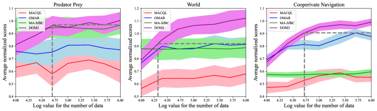
Figure 4: Algorithm performance on data-efficiency.

Ablation study

In this part, we present an ablation study for DOM2, to evaluate its sensitivity to key hyperparameters, including the regularization coefficient value $\eta$ and the diffusion step $N$.

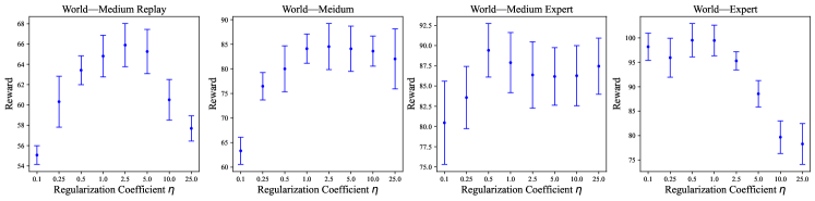
Figure 5: Ablation study on the $\eta$ value in MPE World in $4$ different datasets.

The effect of the regularization coefficient $\eta$

Fig. 5 shows the average score of DOM2 over the MPE world task with different values of the regularization coefficient $\eta\in[0.1,25.0]$ in 4 datasets. In order to perform the advantage of the diffusion-based policy, the appropriate coefficient value $\eta$ needs to balance the two regularization terms appropriately, which is influenced by the performance of the dataset. For the expert dataset, $\eta$ tends to be small, and in other datasets, $\eta$ tends to be relatively larger. The reason that small $\eta$ performs well in the expert dataset is that with data from well-trained strategies, getting close to the behavior policy is sufficient for training a policy without policy improvement.

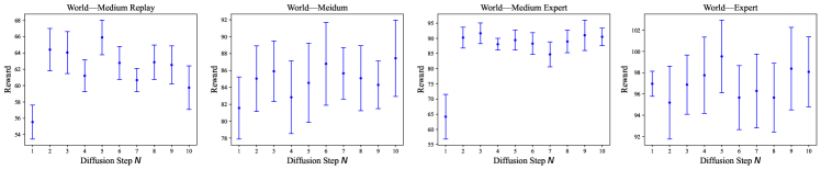
Figure 6: Ablation study on the diffusion step $N$ in MPE World in 4 different datasets.

The effect of the diffusion step $N$

Fig. 6 shows the average score of DOM2 over the MPE world task with different values of the diffusion step $N\in[1,10]$ under each dataset. The numbers of optimal diffusion steps vary with the dataset. We also observe that $N=5$ is a good choice for both efficiency of diffusion action generation and the performance of the obtained policy in MPE.

5.3 Scalability in Multi-Agent MuJoCo Environment

We now turn to the more complex continuous control tasks HalfCheetah-v2 environment in a multi-agent setting (extension of the single-agent task Peng et al. (2021)) and the details are in Appendix B.1.

Performance.

Table 3 shows the performance of DOM2 in the multi-agent HalfCheetah-v2 environments. We see that DOM2 outperforms other compared algorithms and achieves state-of-the-art performances in all the algorithms and datasets.

Table 3: Performance comparison of DOM2 with MA-CQL, OMAR, and MA-SfBC.

HalfCheetah-v2	MA-CQL	OMAR	MA-SfBC	DOM2
Medium Replay	1216.6$\pm$514.6	1674.8$\pm$201.5	-128.3$\pm$71.3	2564.3$\pm$216.9
Medium	963.4$\pm$316.6	2797.0$\pm$445.7	1386.8$\pm$248.8	2851.2$\pm$145.5
Medium Expert	1989.8$\pm$685.6	2900.2$\pm$403.2	1392.3$\pm$190.3	2919.6$\pm$252.8
Expert	2722.8$\pm$1022.6	2963.8$\pm$410.5	2386.6$\pm$440.3	3676.6$\pm$248.1

Generalization.

As in the MPE case, we also evaluate the generalization capability of DOM2 in this setting. Specifically, we design shifted environments following the scheme in Packer et al. (2018), i.e., we set up Random (R) and Extreme (E) environments by changing the environment parameters (details are shown in Appendix B.1). The performance of the algorithms is shown in Table 4. The results show that DOM2 significantly outperforms other algorithms in nearly all settings, and achieves the best performance in $7$ out of $8$ settings.

Table 4: Performance comparison in shifted environments. We use the abbreviation "R" for Random environments and "E" for Extreme environments.

HalfCheetah-v2-R	MA-CQL	OMAR	MA-SfBC	DOM2
Medium Replay	1279.6$\pm$305.4	1648.0$\pm$132.6	-171.4$\pm$43.7	2290.8$\pm$128.5
Medium	1111.7$\pm$585.9	2650.0$\pm$201.5	1367.6$\pm$203.9	2788.5$\pm$112.9
Medium Expert	1291.5$\pm$408.3	2616.6$\pm$368.8	1442.1$\pm$218.9	2731.7$\pm$268.1
Expert	2678.2$\pm$900.9	2295.0$\pm$357.2	2397.4$\pm$670.3	3178.7$\pm$370.5
HalfCheetah-v2-E	MA-CQL	OMAR	MA-SfBC	DOM2
Medium Replay	1290.4$\pm$230.8	1549.9$\pm$311.4	-169.8$\pm$50.5	1904.2$\pm$201.8
Medium	1108.1$\pm$944.0	2197.4$\pm$95.2	1355.0$\pm$195.7	2232.4$\pm$215.1
Medium Expert	1127.1$\pm$565.2	2196.9$\pm$186.9	1393.7$\pm$347.7	2219.0$\pm$170.7
Expert	2117.0$\pm$524.0	1615.7$\pm$707.6	2757.2$\pm$200.6	2641.3$\pm$382.9

6 Conclusion

We propose DOM2, a novel offline MARL algorithm, which contains three key components, i.e., a diffusion mechanism for enhancing policy expressiveness and diversity, an appropriate regularizer, and a data-augmentation method. Through extensive experiments on multi-agent particle and multi-agent MuJoCo environments, we show that DOM2 significantly outperforms state-of-the-art benchmarks. Moreover, DOM2 possesses superior generalization capability and ultra-high data efficiency, i.e., achieving the same performance as benchmarks with $20+$ times less data.

[section] [section]l1

Appendix A Additional Details about Diffusion Probabilistic Model

In this section, we elaborate on more details about the diffusion probabilistic model that we do not cover in Section 4.1 due to space limitation, and compare the similar parts between the diffusion model and DOM2 in offline MARL.

In the noising action part, we emphasize a forward process $\{\bm{b}_{t,j}^{\tau}\}_{\tau\in[\tau_{0},\tau_{N}]}$ starting at $\bm{b}_{t,j}^{\tau_{0}}\sim\bm{\pi}_{\bm{\theta}_{j}}(\cdot|\bm{o}_{t,j})$ in the dataset $\mathcal{D}$ and $\bm{b}_{t,j}^{\tau_{N}}$ is the final noise. This forward process satisfies that for any diffusing time index $\tau\in[\tau_{0},\tau_{N}]$, the transition probability $q_{\tau_{0}\tau}(\bm{b}_{t,j}^{\tau}|\bm{b}_{t,j}^{\tau_{0}})=\mathcal{N}(\bm{b}_{t,j}^{\tau};\alpha_{\tau}\bm{b}_{t,j}^{\tau_{0}},\sigma_{\tau}^{2}\bm{I})$ Lu et al. [2022] ($\alpha_{\tau},\sigma_{\tau}$ is called the noise schedule). We build the reverse process of SDE as Eq. (2) and we will describe the connection between the forward process and the reverse process of SDE. Kingma Kingma et al. [2021] proves that the following forward SDE (Eq. (6)) solves to a process whose transition probability $q_{\tau_{0}\tau}(\bm{b}_{t,j}^{\tau}|\bm{b}_{t,j}^{\tau_{0}})$ is the same as the forward process, which is written as:

$${\rm{d}}\bm{b}^{\tau}_{t,j}=f(\tau)\bm{b}_{t,j}^{\tau}{\rm{d}}\tau+g(\tau){\rm{d}}\bm{w}_{\tau},\quad\bm{b}^{\tau_{0}}_{t,j}\sim\bm{\pi}_{\bm{\beta}_{j}}(\cdot|\bm{o}_{t,j}).$$ (6)

Here $\bm{\pi}_{\bm{\beta}_{j}}(\cdot|\bm{o}_{t,j})$ is the behavior policy to generate $\bm{b}_{t,j}^{\tau_{0}}$ for agent $j$ given the observation $\bm{o}_{t,j}$, $f(\tau)=\frac{{\rm{d}}\log\alpha_{\tau}}{{\rm{d}}\tau},g^{2}(\tau)=\frac{{\rm{d}}\sigma_{\tau}^{2}}{{\rm{d}}\tau}-2\frac{{\rm{d}}\log\alpha_{\tau}}{{\rm{d}}\tau}\sigma_{\tau}^{2}$ and ${\bm{w}}_{t}$ is a standard Brownion motion. It was proven in [Song et al., 2020a] that the forward process of SDE from $\tau_{0}$ to $\tau_{N}$ has an equivalent reverse process of the SDE from $\tau_{N}$ to $\tau_{0}$, which is the Eq. (2). In this way, the forward process of conditional probability and the reverse process of SDE are connected.

In our DOM2 for offline MARL, we propose the objective function in Eq. (3) and its simplification. In detail, following Lu et al. [2022], the loss function for score matching is defined as:

$$\mathcal{L}_{bc}({\bm{\theta}_{j}}) :=\int_{\tau_{0}}^{\tau_{N}}\omega(\tau)\mathbb{E}_{\bm{a}_{t,j}^{\tau}\sim q_{\tau}(\bm{b}_{t,j}^{\tau})}[\|\bm{\epsilon}_{\bm{\theta}_{j}}(\bm{a}_{t,j}^{\tau},\bm{o}_{t,j},\tau)+\sigma_{\tau}\nabla_{\bm{b}_{t,j}^{\tau}}\log q_{\tau}(\bm{b}_{t,j}^{\tau}|\bm{o}_{t,j})\|_{2}^{2}]{\rm{d}}\tau$$ (7)

$$=\int_{\tau_{0}}^{\tau_{N}}\omega(\tau)\mathbb{E}_{\bm{a}_{t,j}^{\tau_{0}}\sim\bm{\pi}_{\bm{\beta}_{j}}(\bm{a}_{t,j}^{\tau_{0}}|\bm{o}_{t,j}),\epsilon\sim\mathcal{N}(\bm{0},\bm{I})}[\|\bm{\epsilon}-\bm{\epsilon}_{\bm{\theta}_{j}}(\alpha_{\tau}\bm{a}_{t,j}^{\tau_{0}}+\sigma_{\tau}\bm{\epsilon},\bm{o}_{t,j},\tau)\|_{2}^{2}]{\rm{d}}\tau+C,$$

where $\omega(\tau)$ is the weighted parameter and $C$ is a constant independent of $\bm{\theta}_{j}$. In practice for simplification, we set that $w(\tau)=1/(\tau_{N}-\tau_{0})$, replace the integration by random sampling a diffusion timestep and ignore the equally weighted parameter $\omega(\tau)$ and the constant $C$. After these simplifications, the final objective becomes Eq. (3).

Next, we introduce the accelerated sampling method to build the connection between the reverse process of SDE for sampling and the accelerated DPM-solver.

In the denoising part, we utilize the following SDE of the reverse process (Eq. (2.5) in Lu et al. [2022]) as:

$${\rm{d}}\bm{a}^{\tau}_{t,j}=\left[f(\tau)\bm{a}^{\tau}_{t,j}+\frac{g^{2}(\tau)}{\sigma_{\tau}}\bm{\epsilon}_{\bm{\theta}_{j}}(\bm{a}_{t,j}^{\tau},\bm{o}_{t,j},\tau)\right]{\rm{d}}\tau+g(\tau){\rm{d}}\overline{\bm{w}}_{\tau},\quad\bm{a}^{\tau_{N}}_{t,j}\sim\mathcal{N}(\bm{0},\bm{I}).$$ (8)

To achieve faster sampling, Song Song et al. [2020a] proves that the following ODE equivalently describes the process given by the reverse diffusion SDE. It is thus called the diffusion ODE.

$$\frac{{\rm{d}}\bm{a}_{t,j}^{\tau}}{{\rm{d}}\tau}=f(\tau)\bm{a}_{t,j}^{\tau}+\frac{g^{2}(\tau)}{2\sigma_{\tau}}\bm{\epsilon}_{\bm{\theta}_{j}}(\bm{a}_{t,j}^{\tau},\bm{o}_{t,j},\tau),\quad\bm{a}^{\tau_{N}}_{t,j}\sim\mathcal{N}(\bm{0},\bm{I}).$$ (9)

At the end of the denoising part, we use the efficient DPM-solver (Eq. (4)) to solve the diffusion ODE and thus implement the denoising process. The formal derivation can be found on Lu et al. [2022] and we restate their argument here for the sake of completeness, for a more detailed explanation, please refer to Lu et al. [2022].

For such a semi-linear structured ODE in Eq. (9), the solution at time $\tau$ can be formulated as:

$$\bm{a}_{t,j}^{\tau}=\exp{\left(\int_{\tau^{\prime}}^{\tau}f(u){\rm{d}}u\right)\bm{a}_{t,j}^{\tau^{\prime}}}+\int_{\tau^{\prime}}^{\tau}\left(\exp{\left(\int_{u}^{\tau}f(z){\rm{d}}z\right)}\frac{g^{2}(u)}{2\sigma_{u}}\bm{\epsilon}_{\bm{\theta}_{j}}(\bm{a}_{t,j}^{u},\bm{o}_{t,j},u)\right){\rm{d}}u.$$ (10)

Defining $\lambda_{\tau}=\log(\alpha_{\tau}/\sigma_{\tau})$, we can rewrite the solution as:

$$\bm{a}_{t,j}^{\tau}=\frac{\alpha_{\tau}}{\alpha_{\tau}^{\prime}}\bm{a}_{t,j}^{\tau^{\prime}}-\alpha_{\tau}\int_{\tau^{\prime}}^{\tau}\left(\frac{{\rm{d}}\lambda_{u}}{{\rm{d}}u}\right)\frac{\sigma_{u}}{\alpha_{u}}\bm{\epsilon}_{\bm{\theta}_{j}}(\bm{a}_{t,j}^{u},\bm{o}_{t,j},u){\rm{d}}u.$$ (11)

Notice that the definition of $\lambda_{\tau}$ is dependent on the noise schedule $\alpha_{\tau},\sigma_{\tau}$. If $\lambda_{\tau}$ is a continuous and strictly decreasing function of $\tau$ (the selection of our final noise schedule in Eq. (13) actually satisfies this requirement, which we will discuss afterwards), we can rewrite the term by change-of-variable. Based on the inverse function $\tau_{\lambda}(\cdot)$ from $\lambda$ to $\tau$ such that $\tau=\tau_{\lambda}(\lambda_{\tau})$ (for simplicity we can also write this term as $\tau_{\lambda}$) and define $\hat{\bm{\epsilon}}_{\bm{\theta}_{j}}(\hat{\bm{a}}_{t,j}^{\lambda_{\tau}},\bm{o}_{t,j},\lambda_{\tau})=\bm{\epsilon}_{\bm{\theta}_{j}}(\bm{a}_{t,j}^{\tau},\bm{o}_{t,j},\tau)$, we can rewrite Eq. (11) as:

$$\bm{a}_{t,j}^{\tau}=\frac{\alpha_{\tau}}{\alpha_{\tau}^{\prime}}\bm{a}_{t,j}^{\tau^{\prime}}-\alpha_{\tau}\int_{\lambda_{\tau^{\prime}}}^{\lambda_{\tau}}\exp{(-\lambda)}\hat{\bm{\epsilon}}_{\bm{\theta}_{j}}(\hat{\bm{a}}_{t,j}^{\lambda},\bm{o}_{t,j},\lambda){\rm{d}}\lambda.$$ (12)

Eq. (12) is satisfied for any $\tau,\tau^{\prime}\in[\tau_{0},\tau_{N}]$. We uniformly partition the diffusion horizon $[\tau_{0},\tau_{N}]$ into $N$ subintervals $\{[\tau_{i},\tau_{i+1}]\}_{i=0}^{N-1}$, where $\tau_{i}=i/N$ (also $\tau_{0}=0,\tau_{N}=1$). We follow Xiao et al. [2021] to use the variance-preserving (VP) type function Ho et al. [2020], Song et al. [2020a], Lu et al. [2022] to train the policy efficiently. First, define $\{\beta_{\tau}\}_{\tau\in[0,1]}$ by

$$\beta_{\tau}=1-\exp\left(-\beta_{\min}\frac{1}{(N+1)}-(\beta_{\max}-\beta_{\min})\frac{2N\tau+1}{2(N+1)^{2}}\right),$$ (13)

and we pick $\beta_{\min}=0.1,\beta_{\max}=20.0$. Then we choose the noise schedule $\alpha_{\tau_{i}},\sigma_{\tau_{i}}$ by $\alpha_{\tau_{i}}=1-\beta_{\tau_{i}},\sigma_{\tau_{i}}^{2}=1-\alpha_{\tau_{i}}^{2}$ for $i=1\dots N$. It can be then verified that by plugging this particular choice of $\alpha_{\tau}$ and $\sigma_{\tau}$ into $\lambda_{\tau}=\log(\alpha_{\tau}/\sigma_{\tau})$, the obtained $\lambda_{\tau}$ is a strictly decreasing function of $\tau$ (Appendix E in Lu et al. [2022]).

In each interval $[\tau_{i-1},\tau_{i}]$, given $\bm{a}_{t,j}^{\tau_{i}}$, the action obtained in the previous diffusion step at $\tau_{i}$, according to Eq. (12), the exact action next step $\bm{a}_{t,j}^{\tau_{i-1}}$ is given by:

$$\bm{a}_{t,j}^{\tau_{i-1}}=\frac{\alpha_{\tau_{i-1}}}{\alpha_{\tau_{i}}}\bm{a}_{t,j}^{\tau_{i}}-\alpha_{\tau_{i}}\int_{\lambda_{\tau_{i}}}^{\lambda_{\tau_{i-1}}}\exp{(-\lambda)}\hat{\bm{\epsilon}}_{\bm{\theta}_{j}}(\hat{\bm{a}}_{t,j}^{\lambda},\bm{o}_{t,j},\lambda){\rm{d}}\lambda.$$ (14)

We denote the $k$-th order derivative of $\hat{\bm{\epsilon}}_{\bm{\theta}_{j}}(\hat{\bm{a}}_{t,j}^{\lambda},\bm{o}_{t,j},\lambda)$ at $\lambda_{\tau_{i}}$, which is written as $\hat{\bm{\epsilon}}_{\bm{\theta}_{j}}^{(k)}(\hat{\bm{a}}_{t,j}^{\lambda},\bm{o}_{t,j},\lambda_{\tau_{i}})$. By ignoring the higher-order remainder $\mathcal{O}((\lambda_{\tau_{i-1}}-\lambda_{\tau_{i}})^{k+1})$, the $k$-th order DPM-solver for sampling can be written as:

$$\bm{a}_{t,j}^{\tau_{i-1}}=\frac{\alpha_{\tau_{i-1}}}{\alpha_{\tau_{i}}}\bm{a}_{t,j}^{\tau_{i}}-\alpha_{\tau_{i}}\sum_{n=0}^{k-1}\hat{\bm{\epsilon}}_{\bm{\theta}_{j}}^{(n)}(\hat{\bm{a}}_{t,j}^{\lambda_{\tau_{i}}},\bm{o}_{t,j},\lambda_{\tau_{i}})\int_{\lambda_{\tau_{i}}}^{\lambda_{\tau_{i-1}}}\exp{(-\lambda)}\frac{(\lambda-\lambda_{\tau_{i}})^{n}}{n!}{\rm{d}}\lambda.$$ (15)

For $k=1$, the results are actually the first-order iteration function in Section 4.1. Similarly, we can use a higher-order DPM-solver.

Appendix B Experimental Details

B.1 Experimental Setup: Environments

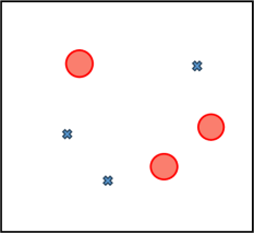
(a) Cooperative Navigation

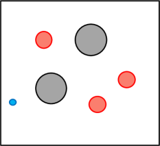
(b) Predator Prey

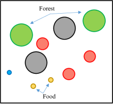
(c) World

(d) 2-Agent HalfCheetah

Figure 7: Multi-agent particle environments (MPE) and Multi-agent HalfCheetah Environment-MuJoCo (MAMuJoCo).

We implement our algorithm and baselines based on the open-source environmental engines of multi-agent particle environments (MPE) Lowe et al. [2017], and multi-agent MuJoCo environments (MAMuJoCo)Peng et al. [2021]. Figure 7 shows the tasks from MPE and MAMuJoCo. In cooperative navigation shown in Fig. 7a, agents (red dots) cooperate to reach the landmark (blue crosses) without collision. In predator-prey in Fig. 7b, predators (red dots) are intended to catch the prey (blue dots) and avoid collision with the landmark (grey dots). The predators need to cooperate with each other to surround and catch the prey because the predators run slower than the prey. The world task in Fig. 7c consists of $3$ agents (red dots) and $1$ adversary (blue dots). The slower agents are intended to catch the faster adversary that desires to eat food (yellow dots). The agents need to avoid collision with the landmark (grey dots). Moreover, if the adversary hides in the forest (green dots), it is harder for the agents to catch the adversary because they do not know the position of the adversary. The two-agent HalfCheetah is shown in Fig. 7d, and different agents control different joints (grey or white joints) and they need to cooperate for better control the half-shaped cheetah to run stably and fast. The expert and random scores for cooperative navigation, predator-prey, and world are $\{516.8,159.8\},\{185.6,-4.1\},\{79.5,-6.8\}$, and we use these scores to calculate the normalized scores in Fig. 4.

For the MAMuJoCo environment, we design two different shifted environments: Random (R) environment and Extreme (E) environments following Packer et al. [2018]. These environments have different parameters and we focus on randomly sampling the three parameters: (1) power, the parameter to influence the force that is multiplied before application, (2) torso density, the parameter to influence the weight, (3) sliding friction of the joints. The detailed sample regions of these parameters in different environments are shown in table 5.

Table 5: Range of parameters in the Multi-MuJoCo HalfCheetah-v2 environment.

	Deterministic	Random	Extreme
Power	1.0	[0.8,1.2]	[0.6,0.8]$\cup$[1.2,1.4]
Density	1000	[750,1250]	[500,750]$\cup$[1250,1500]
Friction	0.4	[0.25,0.55]	[0.1,0.25]$\cup$[0.55,0.7]

B.2 Experimental Setup: Network Structures and Hyperparameters

In DOM2, we utilize the multi-layer perceptron (MLP) to model the Q-value functions of the critics by concatenating the state-action pairs and sending them into the MLP to generate the Q-function, which is the same as in MA-CQL and OMAR Pan et al. [2022]. Different from MA-CQL and OMAR, we use the diffusion policy to generate actions, and we use the U-Net architecture Chen et al. [2022] to model the score function $\bm{\epsilon}_{\bm{\theta}_{j}}(\bm{a}_{t,j}^{\tau_{i}},\bm{o}_{t,j},\tau_{i})$ for agent $j$ at timestep $\tau_{i}$. Different from MA-SfBC Chen et al. [2022], we use the U-Net architecture with a dropout layer for better training stability.

All the MLPs consist of $1$ batch normalization layer, $2$ hidden layers, and $1$ output layer with the size $(\mathrm{input\_dim},\mathrm{hidden\_dim}),(\mathrm{hidden\_dim},\mathrm{hidden\_dim}),(\mathrm{hidden\_dim},\mathrm{output\_dim})$ and $\mathrm{hidden\_dim}=256$. In the hidden layers, the output is activated with the $\mathrm{Mish}$ function, and the output of the output layer is activated with the $\mathrm{Tanh}$ function. The U-Net architecture resembles Janner et al. [2022], Chen et al. [2022] with multiple residual networks as shown in Figure 8. We also introduce a dropout layer after the output of each residual layer with a $0.1$ dropout rate to prevent overfitting.

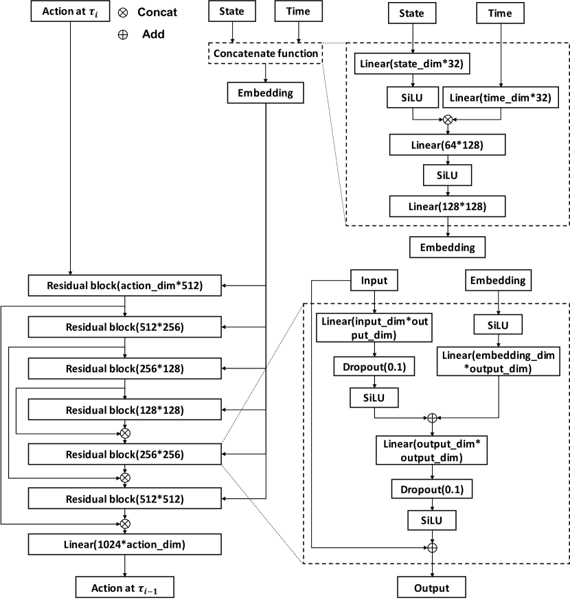
Figure 8: Architecture of the U-Net Ho et al. [2020], Chen et al. [2022] representing $\bm{\epsilon}_{\bm{\theta}_{j}}$, where we include a dropout layer for training stability.

We use $5\times 10^{-3}$ in all MPE environments as the learning rate to train the network of the score function (Fig. 8) in the diffusion policy. For training the Q-value network, we use the learning rate of $3\times 10^{-4}$ in all environments. The trade-off parameter $\eta$ is used to balance the regularizers of actor losses, and the total diffusion step number $N$ is for sampling denoised actions. In the MAMuJoCo HalfCheetah-v2 environment, the learning rates for training the network of the score function in medium-replay, medium, medium-expert, and expert datasets are set to $1\times 10^{-4},2.5\times 10^{-4},2.5\times 10^{-4},5\times 10^{-4}$, respectively. We use $N=5$ as the diffusion timestep in MPE and $N=10$ in the MAMuJoCo HalfCheetah-v2 environment. The hyperparameter $\eta$ and the set of threshold values $\mathcal{R}=\{r_{\text{th},1},...,r_{\text{th},K}\}$ in different settings are shown in table 6. For all other hyperparameters, we use the same values in our experiments.

Table 6: The $\eta$ value and the set of threshold values $\mathcal{R}$ in DOM2.

Predator Prey	$\eta$	Set of threshold values $\mathcal{R}$
Medium Replay	$5.0$	$[0.0,10.0,20.0,30.0,40.0,50.0,60.0,70.0,80.0,90.0,100.0]$
Medium	$2.5$	$[100.0,150.0,200.0,250.0,300.0]$
Medium Expert	$25.0$	$[100.0,150.0,200.0,250.0,300.0,350.0,400.0]$
Expert	$0.5$	$[200.0,250.0,300.0,350.0,400.0]$
World	$\eta$	Set of threshold values $\mathcal{R}$
Medium Replay	$2.5$	$[-3.7,5.9,15.6,15.6]$
Medium	$0.5$	$[65.5,86.4,101.5,101.5]$
Medium Expert	$0.5$	$[50.0,75.0,100.0,125.0,150.0,175.0]$
Expert	$0.5$	$[75.0,100.0,125.0,150.0,175.0]$
Cooperative Navigation	$\eta$	Set of threshold values $\mathcal{R}$
Medium Replay	$500.0$	$[0.0,10.0,20.0,30.0,40.0,50.0,60.0,70.0,80.0,90.0,100.0]$
Medium	$250.0$	$[200.0,250.0,300.0,350.0,400.0,450.0,500.0,550.0]$
Medium Expert	$250.0$	$[264.4,267.3,333.5,336.4,385.3,385.3,387.9,387.9]$
Expert	$50.0$	$[525.0,550.0,575.0,600.0,625.0]$
HalfCheetah-v2	$\eta$	Set of threshold values $\mathcal{R}$
Medium Replay	$1.0$	$[100.0,300.0,500.0,1000.0,1500.0]$
Medium	$2.5$	$[1800.0,1850.0,1900.0,1950.0,2000.0]$
Medium Expert	$2.5$	$[1631.6,1692.5,1735.5,1735.5]$
Expert	$0.05$	$[3800.0,3850.0,3900.0,3950.0,4000.0]$

B.3 Details about 3-Agent 6-Landmark Task

We now discuss detailed results in the $3$-Agent $6$-Landmark task. We construct the environment based on the cooperative navigation task in multi-agent particles environment Lowe et al. [2017]. This task contains $3$ agents and $6$ landmarks. The size of agents and landmarks are all $0.1$. For any landmark $j=0,1,...,5$, its position is given by $(\cos{(\frac{2\pi j}{6})},\sin{(\frac{2\pi j}{6})})$. In each episode, the environment initializes the positions of $3$ agents inside the circle of the center $(0,0)$ with a $0.1$ radius uniformly at random. If the agent can successfully find any one of the landmarks, the agent gains a positive reward. If two agents collide, the agents are both penalized with a negative reward.

We construct two different environments: the standard environment and shifted environment. In the standard environment, all $6$ landmarks exist in the environment, while in the shifted environment, in each episode, we randomly hide $3$ out of $6$ landmarks. We collect data generated from the standard environment and train the agents using different algorithms for both environments.

We evaluate how our algorithm performs compared to the baseline algorithms in this task (with different configurations of the targets) and investigate their performance by rolling out $K$ times at each evaluation ($K\in\{1,10\}$) following Kumar et al. [2020b]. For evaluating the policy in the standard environment, we test the policy for $10$ episodes with different initialized positions and calculate the mean value and the standard deviation as the results of evaluating the policy. This corresponds to rolling out $K=1$ time at each evaluation. For the shifted environment, in spite of the former evaluation method ($K=1$), we also evaluate the algorithm in another way following Kumar et al. [2020b]. We first test the policy for $10$ episodes at the same initialized positions and take the maximum return in these $10$ episodes. We repeat this procedure 10 times with different initialized positions and calculate the mean value and the standard deviation as the results of evaluating the policy, which corresponds to rolling out $K=10$ times at each evaluation. It has been reported (see e.g. Kumar et al. [2020b]) that for a diversity-driven method, increasing $K$ can help the diverse policy gain higher returns.

In table 7, we show the results of different algorithms in standard environments and shifted environments. It can be seen that DOM2 outperforms other algorithms in both the standard environment and shifted environments. Specifically, in the standard environment, DOM2 outperforms other algorithms. This shows that DOM2 has better expressiveness compared to other algorithms. In the shifted environment, when $K=1$, it turns out that DOM2 already achieves better performance with expressiveness. Moreover, when $K=10$, DOM2 significantly improves the performance compared to the results in the $K=1$ setting. This implies that DOM2 finds much more diverse policies, thus achieving better performance compared to the existing conservatism-based method, i.e., MA-CQL and OMAR.

In Fig. 9 (same as Fig. 1b), we show the average mean value and the standard deviation value of different datasets in the standard environment as the left diagram and in the shifted environment with $10$-times evaluation in each episode as the right diagram. The performance of DOM2 is shown as the light blue bar. Compared to the MA-CQL as the orange bar and OMAR as the red bar, DOM2 shows a better average performance in both settings, which means that DOM2 efficiently trains the policy with much better expressiveness and diversity.

Table 7: Comparison of DOM2 with other algorithms in $3$-Agent $6$-Landmark settings.

Standard-$K=1$	MA-CQL	OMAR	MA-SfBC	DOM2
Medium Replay	396.9$\pm$40.1	455.7$\pm$52.5	339.3$\pm$29.5	542.4$\pm$32.5
Medium	267.4$\pm$37.2	349.9$\pm$20.7	459.9$\pm$25.2	532.5$\pm$55.2
Medium Expert	300.9$\pm$77.4	395.5$\pm$91.0	552.1$\pm$16.9	678.7$\pm$4.4
Expert	457.5$\pm$110.0	595.0$\pm$54.7	606.1$\pm$13.9	683.3$\pm$2.1
Shifted-$K=1$	MA-CQL	OMAR	MA-SfBC	DOM2
Medium Replay	247.0$\pm$43.4	274.4$\pm$18.0	205.7$\pm$37.5	317.2$\pm$54.7
Medium	171.6$\pm$21.8	214.0$\pm$18.0	276.7$\pm$48.9	284.8$\pm$37.6
Medium Expert	201.2$\pm$54.7	241.9$\pm$32.2	328.7$\pm$45.9	382.3$\pm$36.4
Expert	258.1$\pm$67.5	334.0$\pm$21.7	374.2$\pm$28.5	393.1$\pm$43.3
Shifted-$K=10$	MA-CQL	OMAR	MA-SfBC	DOM2
Medium Replay	253.3$\pm$39.3	294.3$\pm$30.2	288.7$\pm$29.4	357.2$\pm$67.2
Medium	181.9$\pm$21.4	235.7$\pm$33.1	343.7$\pm$32.7	315.5$\pm$37.6
Medium Expert	213.8$\pm$57.4	274.2$\pm$28.5	440.9$\pm$21.8	486.3$\pm$41.6
Expert	277.7$\pm$51.7	358.2$\pm$21.5	470.6$\pm$21.2	487.6$\pm$11.8

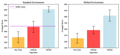
Figure 9: Results of the algorithms in the standard environments (Left) and the shifted environments (Right) of $3$-Agent $6$-Landmark examples.

References

- Lange et al. (2012) Sascha Lange, Thomas Gabel, and Martin Riedmiller. Batch reinforcement learning. In Reinforcement learning, pages 45–73. Springer, 2012.
- Levine et al. (2020) Sergey Levine, Aviral Kumar, George Tucker, and Justin Fu. Offline reinforcement learning: Tutorial, review, and perspectives on open problems. arXiv preprint arXiv:2005.01643, 2020.
- Wu et al. (2019) Yifan Wu, George Tucker, and Ofir Nachum. Behavior regularized offline reinforcement learning. arXiv preprint arXiv:1911.11361, 2019.
- Kumar et al. (2019) Aviral Kumar, Justin Fu, Matthew Soh, George Tucker, and Sergey Levine. Stabilizing off-policy q-learning via bootstrapping error reduction. Advances in Neural Information Processing Systems, 32, 2019.
- Fujimoto et al. (2019) Scott Fujimoto, David Meger, and Doina Precup. Off-policy deep reinforcement learning without exploration. In International conference on machine learning, pages 2052–2062. PMLR, 2019.
- Kumar et al. (2020a) Aviral Kumar, Aurick Zhou, George Tucker, and Sergey Levine. Conservative q-learning for offline reinforcement learning. Advances in Neural Information Processing Systems, 33:1179–1191, 2020a.
- Fujimoto and Gu (2021) Scott Fujimoto and Shixiang Shane Gu. A minimalist approach to offline reinforcement learning. Advances in neural information processing systems, 34:20132–20145, 2021.
- Kostrikov et al. (2021a) Ilya Kostrikov, Rob Fergus, Jonathan Tompson, and Ofir Nachum. Offline reinforcement learning with fisher divergence critic regularization. In International Conference on Machine Learning, pages 5774–5783. PMLR, 2021a.
- Lee et al. (2022) Seunghyun Lee, Younggyo Seo, Kimin Lee, Pieter Abbeel, and Jinwoo Shin. Offline-to-online reinforcement learning via balanced replay and pessimistic q-ensemble. In Conference on Robot Learning, pages 1702–1712. PMLR, 2022.
- Jiang and Lu (2021) Jiechuan Jiang and Zongqing Lu. Offline decentralized multi-agent reinforcement learning. arXiv preprint arXiv:2108.01832, 2021.
- Yang et al. (2021) Yiqin Yang, Xiaoteng Ma, Chenghao Li, Zewu Zheng, Qiyuan Zhang, Gao Huang, Jun Yang, and Qianchuan Zhao. Believe what you see: Implicit constraint approach for offline multi-agent reinforcement learning. Advances in Neural Information Processing Systems, 34:10299–10312, 2021.
- Pan et al. (2022) Ling Pan, Longbo Huang, Tengyu Ma, and Huazhe Xu. Plan better amid conservatism: Offline multi-agent reinforcement learning with actor rectification. In International Conference on Machine Learning, pages 17221–17237. PMLR, 2022.
- Wang et al. (2022) Zhendong Wang, Jonathan J Hunt, and Mingyuan Zhou. Diffusion policies as an expressive policy class for offline reinforcement learning. arXiv preprint arXiv:2208.06193, 2022.
- Ho et al. (2020) Jonathan Ho, Ajay Jain, and Pieter Abbeel. Denoising diffusion probabilistic models. Advances in Neural Information Processing Systems, 33:6840–6851, 2020.
- Song et al. (2020a) Yang Song, Jascha Sohl-Dickstein, Diederik P Kingma, Abhishek Kumar, Stefano Ermon, and Ben Poole. Score-based generative modeling through stochastic differential equations. arXiv preprint arXiv:2011.13456, 2020a.
- Croitoru et al. (2023) Florinel-Alin Croitoru, Vlad Hondru, Radu Tudor Ionescu, and Mubarak Shah. Diffusion models in vision: A survey. IEEE Transactions on Pattern Analysis and Machine Intelligence, 2023.
- Lu et al. (2022) Cheng Lu, Yuhao Zhou, Fan Bao, Jianfei Chen, Chongxuan Li, and Jun Zhu. Dpm-solver: A fast ode solver for diffusion probabilistic model sampling in around 10 steps. arXiv preprint arXiv:2206.00927, 2022.
- Peng et al. (2019) Xue Bin Peng, Aviral Kumar, Grace Zhang, and Sergey Levine. Advantage-weighted regression: Simple and scalable off-policy reinforcement learning. arXiv preprint arXiv:1910.00177, 2019.
- Siegel et al. (2020) Noah Y Siegel, Jost Tobias Springenberg, Felix Berkenkamp, Abbas Abdolmaleki, Michael Neunert, Thomas Lampe, Roland Hafner, Nicolas Heess, and Martin Riedmiller. Keep doing what worked: Behavioral modelling priors for offline reinforcement learning. arXiv preprint arXiv:2002.08396, 2020.
- Nair et al. (2020) Ashvin Nair, Abhishek Gupta, Murtaza Dalal, and Sergey Levine. Awac: Accelerating online reinforcement learning with offline datasets. arXiv preprint arXiv:2006.09359, 2020.
- Swaminathan and Joachims (2015) Adith Swaminathan and Thorsten Joachims. Batch learning from logged bandit feedback through counterfactual risk minimization. The Journal of Machine Learning Research, 16(1):1731–1755, 2015.
- Liu et al. (2019) Yao Liu, Adith Swaminathan, Alekh Agarwal, and Emma Brunskill. Off-policy policy gradient with state distribution correction. arXiv preprint arXiv:1904.08473, 2019.
- Nachum et al. (2019) Ofir Nachum, Bo Dai, Ilya Kostrikov, Yinlam Chow, Lihong Li, and Dale Schuurmans. Algaedice: Policy gradient from arbitrary experience. arXiv preprint arXiv:1912.02074, 2019.
- Kostrikov et al. (2021b) Ilya Kostrikov, Ashvin Nair, and Sergey Levine. Offline reinforcement learning with implicit q-learning. arXiv preprint arXiv:2110.06169, 2021b.
- Rezaeifar et al. (2022) Shideh Rezaeifar, Robert Dadashi, Nino Vieillard, Léonard Hussenot, Olivier Bachem, Olivier Pietquin, and Matthieu Geist. Offline reinforcement learning as anti-exploration. In Proceedings of the AAAI Conference on Artificial Intelligence, volume 36, pages 8106–8114, 2022.
- Oliehoek et al. (2008) Frans A Oliehoek, Matthijs TJ Spaan, and Nikos Vlassis. Optimal and approximate q-value functions for decentralized pomdps. Journal of Artificial Intelligence Research, 32:289–353, 2008.
- Matignon et al. (2012) Laëtitia Matignon, Laurent Jeanpierre, and Abdel-Illah Mouaddib. Coordinated multi-robot exploration under communication constraints using decentralized markov decision processes. In Twenty-sixth AAAI conference on artificial intelligence, 2012.
- Lowe et al. (2017) Ryan Lowe, Yi I Wu, Aviv Tamar, Jean Harb, OpenAI Pieter Abbeel, and Igor Mordatch. Multi-agent actor-critic for mixed cooperative-competitive environments. Advances in neural information processing systems, 30, 2017.
- Ackermann et al. (2019) Johannes Ackermann, Volker Gabler, Takayuki Osa, and Masashi Sugiyama. Reducing overestimation bias in multi-agent domains using double centralized critics. arXiv preprint arXiv:1910.01465, 2019.
- de Witt et al. (2020) Christian Schroeder de Witt, Tarun Gupta, Denys Makoviichuk, Viktor Makoviychuk, Philip HS Torr, Mingfei Sun, and Shimon Whiteson. Is independent learning all you need in the starcraft multi-agent challenge? arXiv preprint arXiv:2011.09533, 2020.
- Yu et al. (2021) Chao Yu, Akash Velu, Eugene Vinitsky, Yu Wang, Alexandre Bayen, and Yi Wu. The surprising effectiveness of ppo in cooperative, multi-agent games. arXiv preprint arXiv:2103.01955, 2021.
- Sunehag et al. (2017) Peter Sunehag, Guy Lever, Audrunas Gruslys, Wojciech Marian Czarnecki, Vinicius Zambaldi, Max Jaderberg, Marc Lanctot, Nicolas Sonnerat, Joel Z Leibo, Karl Tuyls, et al. Value-decomposition networks for cooperative multi-agent learning. arXiv preprint arXiv:1706.05296, 2017.
- Rashid et al. (2018) Tabish Rashid, Mikayel Samvelyan, Christian Schroeder, Gregory Farquhar, Jakob Foerster, and Shimon Whiteson. Qmix: Monotonic value function factorisation for deep multi-agent reinforcement learning. In International conference on machine learning, pages 4295–4304. PMLR, 2018.
- Sohl-Dickstein et al. (2015) Jascha Sohl-Dickstein, Eric Weiss, Niru Maheswaranathan, and Surya Ganguli. Deep unsupervised learning using nonequilibrium thermodynamics. In International Conference on Machine Learning, pages 2256–2265. PMLR, 2015.
- Song and Ermon (2019) Yang Song and Stefano Ermon. Generative modeling by estimating gradients of the data distribution. Advances in Neural Information Processing Systems, 32, 2019.
- Song et al. (2020b) Jiaming Song, Chenlin Meng, and Stefano Ermon. Denoising diffusion implicit models. arXiv preprint arXiv:2010.02502, 2020b.
- Nichol et al. (2021) Alex Nichol, Prafulla Dhariwal, Aditya Ramesh, Pranav Shyam, Pamela Mishkin, Bob McGrew, Ilya Sutskever, and Mark Chen. Glide: Towards photorealistic image generation and editing with text-guided diffusion models. arXiv preprint arXiv:2112.10741, 2021.
- Ramesh et al. (2022) Aditya Ramesh, Prafulla Dhariwal, Alex Nichol, Casey Chu, and Mark Chen. Hierarchical text-conditional image generation with clip latents. arXiv preprint arXiv:2204.06125, 2022.
- Saharia et al. (2022) Chitwan Saharia, William Chan, Saurabh Saxena, Lala Li, Jay Whang, Emily L Denton, Kamyar Ghasemipour, Raphael Gontijo Lopes, Burcu Karagol Ayan, Tim Salimans, et al. Photorealistic text-to-image diffusion models with deep language understanding. Advances in Neural Information Processing Systems, 35:36479–36494, 2022.
- Chen et al. (2023) Minshuo Chen, Kaixuan Huang, Tuo Zhao, and Mengdi Wang. Score approximation, estimation and distribution recovery of diffusion models on low-dimensional data. arXiv preprint arXiv:2302.07194, 2023.
- Bao et al. (2022) Fan Bao, Chongxuan Li, Jun Zhu, and Bo Zhang. Analytic-dpm: an analytic estimate of the optimal reverse variance in diffusion probabilistic models. arXiv preprint arXiv:2201.06503, 2022.
- Kingma and Welling (2013) Diederik P Kingma and Max Welling. Auto-encoding variational bayes. arXiv preprint arXiv:1312.6114, 2013.
- Janner et al. (2022) Michael Janner, Yilun Du, Joshua B Tenenbaum, and Sergey Levine. Planning with diffusion for flexible behavior synthesis. arXiv preprint arXiv:2205.09991, 2022.
- Ajay et al. (2022) Anurag Ajay, Yilun Du, Abhi Gupta, Joshua Tenenbaum, Tommi Jaakkola, and Pulkit Agrawal. Is conditional generative modeling all you need for decision-making? arXiv preprint arXiv:2211.15657, 2022.
- Chen et al. (2022) Huayu Chen, Cheng Lu, Chengyang Ying, Hang Su, and Jun Zhu. Offline reinforcement learning via high-fidelity generative behavior modeling. arXiv preprint arXiv:2209.14548, 2022.
- Lu et al. (2023) Cheng Lu, Huayu Chen, Jianfei Chen, Hang Su, Chongxuan Li, and Jun Zhu. Contrastive energy prediction for exact energy-guided diffusion sampling in offline reinforcement learning. arXiv preprint arXiv:2304.12824, 2023.
- Oliehoek and Amato (2016) Frans A Oliehoek and Christopher Amato. A concise introduction to decentralized POMDPs. Springer, 2016.
- Hasselt (2010) Hado Hasselt. Double q-learning. Advances in neural information processing systems, 23, 2010.
- Lillicrap et al. (2015) Timothy P Lillicrap, Jonathan J Hunt, Alexander Pritzel, Nicolas Heess, Tom Erez, Yuval Tassa, David Silver, and Daan Wierstra. Continuous control with deep reinforcement learning. arXiv preprint arXiv:1509.02971, 2015.
- Kingma et al. (2021) Diederik Kingma, Tim Salimans, Ben Poole, and Jonathan Ho. Variational diffusion models. Advances in neural information processing systems, 34:21696–21707, 2021.
- Peng et al. (2021) Bei Peng, Tabish Rashid, Christian Schroeder de Witt, Pierre-Alexandre Kamienny, Philip Torr, Wendelin Böhmer, and Shimon Whiteson. Facmac: Factored multi-agent centralised policy gradients. Advances in Neural Information Processing Systems, 34:12208–12221, 2021.
- Fu et al. (2020) Justin Fu, Aviral Kumar, Ofir Nachum, George Tucker, and Sergey Levine. D4rl: Datasets for deep data-driven reinforcement learning. arXiv preprint arXiv:2004.07219, 2020.
- Packer et al. (2018) Charles Packer, Katelyn Gao, Jernej Kos, Philipp Krähenbühl, Vladlen Koltun, and Dawn Song. Assessing generalization in deep reinforcement learning. arXiv preprint arXiv:1810.12282, 2018.
- Xiao et al. (2021) Zhisheng Xiao, Karsten Kreis, and Arash Vahdat. Tackling the generative learning trilemma with denoising diffusion gans. arXiv preprint arXiv:2112.07804, 2021.
- Kumar et al. (2020b) Saurabh Kumar, Aviral Kumar, Sergey Levine, and Chelsea Finn. One solution is not all you need: Few-shot extrapolation via structured maxent rl. Advances in Neural Information Processing Systems, 33:8198–8210, 2020b.
[section] \printcontents[section]l1