Hybrid two-level MCMC for Bayesian Inverse Problems

1 Introduction

Inverse problems arise from various scientific and engineering domains, such as recovering subsurface rock permeability, engineering design parameter optimization, or data assimilation in weather forecasts. Many of those problems are governed by physical laws described by Partial Differential Equations (PDEs) [MR2102218]. We consider the Bayesian inverse problems formulated with Bayes’ rule, which accounts for uncertainties. Bayesian inverse problems can be finite-dimensional, in which only a finite number of parameters are recovered [MR3285819]. However, in many scenarios, scientists and engineers are interested in recovering functions that are considered infinite-dimensional Bayesian inverse problems [MR2652785].
Typically solving such Bayesian inverse problems leads to repeatedly solving the forward problem either in a deterministic approach or a statistical approach. In large-scale PDE-constrained problems, it means running an expensive numerical simulation iteratively. Particularly when dealing with infinite-dimensional Bayesian inverse problems, a high-dimensional numerical system has to be dealt with due to discretization during computation. It also causes various computational challenges due to the curse of dimensionality.
The recent development of deep neural networks has shown promising opportunities for neural network based surrogate models for solving such Bayesian inverse problems effectively. We mention the following references on solving PDE equations with neural networks, including Physics Informed Neural Networks (PINNs), Fourier Neural Operator, DeepONet and etc [MR3881695, DBLP:conf/iclr/LiKALBSA21, lu2021learning]. Examples of PINNs have shown that they can learn the solution of parameterized PDEs and be used for design optimization which is a typical inverse problem. Literature on neural operators has also shown that neural networks can learn linear and nonlinear mappings between functional spaces very well. The fast inference time of neural operators motivated the idea of using trained neural operators as surrogate models. The outstanding performances of neural networks in high-dimensional problems make the use of neural operators even more promising in comparison with classical surrogate models, e.g. polynomial approximations. With such progress, solving inverse problems intractable with classical methods becomes possible.
Despite the advantages of neural network models as surrogate models, neural networks themselves are nonlinear complex models. There is a lack of a rigorous mathematical framework to conclude an error bound of a given model, contrary to the well-understood numerical methods. The majority of the applications take it as a black box and check the results empirically. Though in theory, there is a universal approximation theorem for continuous functions and another universal approximation theorem for operators [chen1995universal], there is often an empirical accuracy ceiling given the complexity of the model and size of the data. Some numerical analysis can be found on the expressivity of ReLU neural networks which depends on the layers and number of connections [petersen2018optimal, aadebffb88b448c89c654fcdda52c02b]. Training the neural network which usually leads to a non-convex optimization problem, the expressivity is not guaranteed as an error rate. In practice, the training of neural networks often requires trial and error with empirical knowledge from experienced data scientists. It is known empirically that increasing AI model accuracy usually requires exponentially more data, known as the power law [hestness2017deep]. It is still not guaranteed that increasing model complexity and data size will always lead to higher accuracy. The limitation hinders the adoption of neural network based models in practical applications, as the error in the surrogate model will lead to the approximation error both in the Quantity of Interest and also the approximation of posterior distribution under the Bayesian framework. We propose a two-level hybrid MCMC approach to solve Bayesian inverse problems with neural network based surrogate models which takes account of the error of the neural network models. In essence, taking advantage of the mathematical framework of the multilevel MCMC methods, this method samples the differences between the neural network model and numerical model with known accuracy with a limited number of numerical samples. This approach will reach the same accuracy as a MCMC chain with expensive numerical solutions by correcting the errors of a plain MCMC approach with only neural network models with limited additional computational cost.

2 Bayesian inverse problem

In this section, we consider the Bayesian inverse problems with a forward mathematical model that predicts the states $u$ of a physical system given parameters $z=\{z_{1},z_{2},...,z_{n}\}$. Here we assume the forward mathematical model governed by partial differential equations with $z$, a finite number of parameters of the governing equation or the coefficients of the spectral expansion of the initial condition or forcing. Some examples are subsurface flow model who depends on the porosity of rocks, elasticity equations who depends on the Lame constants of the material and Navier Stokes equations whose solution depends on the initial condition and forcing. To present the setting for the Bayesian inverse problem, we consider the inverse problem with uniform prior. We denote the probability space $U=[-1,1]^{n}$, and sigma algebra on the domain $U$ by $\Theta=\bigotimes_{j=1}^{n}\mathcal{B}([-1,1])$. we define the forward observation map $\mathcal{G}:U\rightarrow\mathbb{R}^{k}$ for all $z\in U$ as

$$\mathcal{G}(z)=(\mathcal{O}_{1}(u),\mathcal{O}_{2}(u),...,\mathcal{O}_{k}(u)),$$ (1)

where $u$ is the forward solution of the governing PDE equation and $\mathcal{O}_{i},i=1,2,...k$ are $k$ continuous bounded linear functionals.

Assumption 2.1.

The forward map $\mathcal{G}(z):U\rightarrow\mathbb{R}^{k}$ is continuous as a mapping from the measurable space $(U,\Theta)$ to $(\mathbb{R}^{k},\mathcal{B}(\mathbb{R}^{k}))$.

Remark 2.2.

Assumption 2.1 is valid for most PDEs constrained systems. One can find proofs for elliptic equations and parabolic equations in [MR2558668, MR3084684, MR4246090]. Proofs for elasticity equations and Navier Stokes equations can be found in [MR2652785].

Let $\vartheta$ be the observation noise. It is assumed Gaussian and independent of the parameters $z$. Thus the random variable $\vartheta$ has values in $\mathbb{R}^{k}$ and following normal distribution $N(0,\Sigma)$, where $\Sigma$ is a known $k\times k$ symmetric positive covariance matrix. The noisy observation $\delta$ is

$$\delta=\mathcal{G}+\vartheta.$$ (2)

We denote the posterior distribution as $\gamma^{\delta}$ and the prior distribution as $\gamma$.

Proposition 2.3.

The posterior probability measure $\gamma^{\delta}$ is absolutely continuous with respect to the prior $\gamma$. The Randon-Nikodym derivative is given by

$$\frac{d\gamma^{\delta}}{d\gamma}\propto\exp(-\Phi(z;\delta)),$$ (3)

where $\Phi$ is the potential function

$$\Phi(z,\delta)=\frac{1}{2}|\delta-\mathcal{G}(z)|_{\Sigma}^{2}.$$ (4)

The proof of Proposition 2.3 follows naturally from Assumption 2.1. Detailed proof can be found in [MR2652785]. Next we consider the continuity of the posterior measure in the Hellinger distance with respect to the observation data, which implies the well-posedness of the posterior measure. The Hellinger distance is defined as

$$d_{Hell}(\gamma^{\prime},\gamma^{\prime\prime})=\left(\frac{1}{2}\int_{U}\left(\sqrt{\frac{d\gamma^{\prime}}{d\gamma}}-\sqrt{\frac{d\gamma^{\prime\prime}}{d\gamma}}\right)^{2}d\gamma\right)^{\frac{1}{2}},$$ (5)

where $\gamma^{\prime}$ and $\gamma^{\prime\prime}$ are two measures on $U$, which are absolutely continuous with respect to the measure $\gamma$. Following the results in [MR2652785, MR2558668, MR4069815], we know that the Lipschitzness of the posterior measure with respect to the Hellinger distance holds under general conditions, hence the following proposition.

Proposition 2.4.

The measure $\gamma^{\delta}$ depends locally Lipschitz continuously on the data $\delta$ with respect to the Hellinger metric: for every $r>0$ and $\delta,\delta^{\prime}\in\mathbb{R}^{d}$ such that for $|\delta|_{\Sigma},|\delta^{\prime}|_{\Sigma}\leq r$, there exists $C=C(r)>0$ such that

$$d_{Hell}(\gamma^{\delta},\gamma^{\delta^{\prime}})\leq C(r)|\delta-\delta^{\prime}|_{\Sigma}.$$

3 Numerical discretization approximation

We consider classical numerical discretizations of such PDE-constrained forward problems, such as the finite volume method and finite element method. Such numerical approximations errors usually depend on the mesh size. We make the following assumption on the numerical approximation error which is true for problems like FE approximation for elliptic equations, parabolic equations, two dimensional Navier Stokes equations and etc [MR2050138, MR1043610]. See [MR2897628] for the standard error rate of Finite Volume approximation.

Assumption 3.1.

We denote the solution space of $u$ as $V$, where the solution space $V$ is typically $H^{1}$ or $H_{0}^{1}$. Consider the numerical discretization approximation of the forward problem, there is a constant $C>0$ such that for every $l\in\mathbb{N}$ and for every $z\in U$, the following error bound holds

$$\|u-u^{l}\|_{V}\leq C2^{-l},$$ (6)

where $l$ is the level of discretization and the mesh size $h=2^{-l}$.

With the numerical approximation of the forward equation, we consider the approximation of the posterior measure. We denote the numerical approximation of the forward map $\mathcal{G}^{l}:U\rightarrow\mathbb{R}^{k}$ by

$$\mathcal{G}^{l}(z)=(\mathcal{O}_{1}(u^{l}),\mathcal{O}_{2}(u^{l})...,\mathcal{O}_{k}(u^{l})).$$ (7)

The potential function is now $\Phi^{l}(z;\delta)=\frac{1}{2}|\delta-\mathcal{G}^{l}(z)|_{\Sigma}^{2}$. And we define the approximate posterior probability measure $\gamma^{l,\delta}$ on the measurable space $(U,\Theta)$ as

$$\frac{d\gamma^{l,\delta}}{d\gamma}\propto\exp(-\Phi^{l}(z;\delta)).$$

Hence similar to Proposition 2.3, we have the following proposition for the approximate posterior probability measure.

Proposition 3.2.

There exists a postive constant $C(\delta)$ depending only on the data $\delta$ such that for every $l$

$$d_{Hell}(\gamma^{\delta},\gamma^{l,\delta})\leq C(\delta)2^{-l}.$$

4 Machine learning based surrogate model

One of the key challenges for Bayesian inverse problems is the high computational cost. Particularly, statistical approaches such as Markov Chain Monte Carlo method requires solving the forward problem repeatedly. And due to the sequential nature of MCMC method, the forward problem has to be solved for millions of times without a trivial way to parallelize. The surrogate model has been one of the solutions to accelerate the process. With the recent development of neural-network and deep learning, machine learning based surrogate model has been found with good potential to create accurate surrogate models for high dimensional forward problems.[maulik2022efficient] Recent research on Physics Informed Neural-Network and Neural Operators have demonstrated such potentials [MR3881695, MR4395087, DBLP:conf/iclr/LiKALBSA21]. However, domain experts from different communities often have critics of the lack of conservation of physics in the machine learning models. Even with the physics informed models, we see many challenges in training a machine learning model that’s accurate enough due to the soft constraint. In addition, the lack of understanding of the modern deep learning models is also challenging for researchers who care a lot about the model confidence and the estimated error rate. Examples of the residual errors of neural operator in Bayesian inverse problems can be found in [DBLP:journals/corr/abs-2210-03008].

We denote $\tilde{\mathcal{G}}:U\rightarrow\mathbb{R}^{k}$ as a nonlinear map defined by a trained neural network. We assume the neural network model is trained with data generated with classical numerical methods, e.g. Finite element method and finite difference method. We assume the objective to be solving the inverse problem with an error less or equal to $\mathcal{O}(2^{-L})$. The procedure to solve such an inverse problem with machine learning acceleration is as followed. First, we create a numerical model used to generate the data, which is discretized with a fine mesh with mesh size $h$. To achieve the targeted accuracy, we have $h=\mathcal{O}(2^{-L})$. According section 3, we will achieve an accuracy of $\mathcal{O}(2^{-L})$. Second, we use those generated numerical data as training data to train a neural netowrk model. Third, we use the trained machine learning model as a surrogate model to quickly run a MCMC chain. Lastly, according to the theory of MCMC, we will get an estimated expectation of the Quantity of Interest within the desired error if the machine learning model can be as accurate as the numerical model. However, empirically, we are aware that the trained neural network can hardly achieve the same level of accuracy as the numerical model used to generate the training data. Hence we make the following assumption.

Assumption 4.1.

Given a neural network trained by data generated by a numerical model with mesh size $h=2^{-L}$, we have

$$\|\tilde{G}(x)-u\|_{V}\leq 2^{-L+\epsilon},$$

where $x$ is the input and we expect $\epsilon$ to be a small value for a well defined and trained neural network.

We expect the $\epsilon$ to be small in practice when we have a reasonably good machine learning model trained with sufficient data. In order to mitigate the shortcomings of machine learning based surrogate model, one can increase the accuracy of the numerical model used to generate more training data to better train the model in order to reach the desired accuracy. However, that will increase the computational cost by many folds. In general, to solve a two dimensional problem, the minimum increment of the computational cost of the numerical model is 4 times and 8 times for three dimensional problems, not to mention more challenging problems whose computational cost does not scale linearly. In addition to the cost of finer numerical solvers, the need for more data points also will increase the computational cost. The increment of data resolution and size will also increase the cost of training the machine learning model. Even if we are willing to pay the cost, [DBLP:journals/corr/abs-2210-03008] has shown that there is usually a limit on how accurate certain machine learning models can be. [DBLP:journals/corr/abs-2210-03008] also proposed a residual-based error correction to deal with the problem, where a variational model is used to correct the solution of each inference. In the next section, we propose a different approach to correct the error statistically.

5 Hybrid two level MCMC

In this section, we propose the hybrid two level MCMC method for error correction of the machine learning accelerated surrogate model for Bayesian inverse problems. To tackle the high computational cost of MCMC with a numerical solver, Multilevel Markov Chain Monte Carlo (MLMCMC) was developed which in theory is optimal and reduces the computational cost by two order of magnitude for various problems [MR3084684, MR4246090, MR4523340]. Inspired by the multilevel approach, we describe the hybrid two level MCMC method for sampling the posterior probability of the Bayesian inverse problems, in which the base chain is run with a machine learning accelerated surrogate model with a small error and another chain run with a numerical model with known accuracy to correct the statistical error of the machine learning driven MCMC chain.
Similar to the telescoping argument for the multilevel Monte Carlo method [MR2436856], we use the machine learning MCMC chain as the base chain and use another chain to sample the difference between the machine learning model and the numerical model. We denote the Quantity of Interest as $Q$, the machine learning approximate posterior distribution $\gamma^{\rm ML}$, and the numerical approximate posterior distribution $\gamma^{\rm num}$. With the target accuracy of $\mathcal{O}(2^{-L})$ and Assumption 4.1, $\gamma^{\rm ML}$ and $\gamma^{\rm num}$ is equivalent to $\gamma^{L,\delta}$ and $\gamma^{L-\epsilon,\delta}$ in section 3. With the two level approach, we can rewrite the numerical approximation of the expected Quantity of Interest as

$$\mathbb{E}^{\gamma^{\rm num}}[Q] =\mathbb{E}^{\gamma^{\rm num}}[Q]-\mathbb{E}^{\gamma^{\rm ML}}[Q]+\mathbb{E}^{\gamma^{ML}}[Q]$$

$$=\left(\mathbb{E}^{\gamma^{\rm num}}-\mathbb{E}^{\gamma^{\rm ML}}\right)[Q]+\mathbb{E}^{\gamma^{ML}}[Q].$$ (8)

To derive a computable estimator with MCMC chains, we observe the first term in (5) can be transformed as such,

$$\left(\mathbb{E}^{\gamma^{\rm num}}-\mathbb{E}^{\gamma^{\rm ML}}\right)[Q] =\frac{1}{Z^{\rm num}}\int_{U}\exp(-\Phi^{\rm num})Qd\gamma-\frac{1}{Z^{\rm ML}}\int_{U}\exp(-\Phi^{\rm ML})Qd\gamma$$

$$=\frac{1}{Z^{\rm num}}\int_{U}\exp(-\Phi^{\rm num})(1-\exp(\Phi^{\rm num}-\Phi^{\rm ML}))Qd\gamma$$

$$+(\frac{Z^{\rm ML}}{Z^{\rm num}}-1)\frac{1}{Z^{\rm ML}}\int_{U}\exp(-\Phi^{\rm ML})Qd\gamma.$$ (9)

We note that the constant $(\frac{Z^{\rm ML}}{Z^{\rm num}}-1)$ can be expanded as following which can be approximated with a MCMC chain,

$$(\frac{Z^{\rm ML}}{Z^{\rm num}}-1)=\frac{1}{Z^{\rm num}}\int_{U}(\exp(\Phi^{\rm num}-\Phi^{\rm ML})-1)\exp(-\Phi^{\rm num})d\gamma.$$ (10)

Hence with (5), (6) and (10), we can define the hybrid two level MCMC estimator $\mathbf{E}^{\rm hybrid}[Q]$ of $\mathbb{E}^{\gamma^{\delta}}[Q]$ as

$$\mathbf{E}^{\rm hybrid}[Q] =\mathbf{E}^{\gamma^{\rm num}}_{M_{\rm num}}[(1-\exp(\Phi^{\rm num}-\Phi^{\rm ML}))Q]$$

$$+\mathbf{E}^{\gamma^{\rm num}}_{M_{\rm num}}[\exp(\Phi^{\rm num}-\Phi^{\rm ML})-1]\cdot\mathbf{E}^{\gamma^{\rm ML}}_{M_{\rm ML}}[Q]+\mathbf{E}_{M_{\rm ML}}^{\gamma^{\rm ML}}[Q].$$ (11)

Up to this point, we have constructed the hybrid two level MCMC method for Bayesian inverse problems. The hybrid two level MCMC approach is surprisingly simple. Next we will show the error analysis where we will see it will effectively correct the estimator error caused by machine learning models. To estimate the error, we decompose the error into three components as follows.

Proposition 5.1.

The estimator error holds as such,

$$\mathbb{E}^{\gamma^{\delta}}[Q]-\mathbf{E}^{\rm hybrid}[Q]=I+II+III,$$

where

$$I:=\mathbb{E}^{\gamma^{\delta}}[Q]-\mathbb{E}^{\gamma^{\rm num}}[Q],\quad II:=\mathbb{E}^{\gamma^{ML}}[Q]-\mathbf{E}^{\gamma^{ML}}_{M_{\rm ML}}[Q]$$

and

$$III :=\mathbb{E}^{\gamma^{\rm num}}[(1-\exp(\Phi^{\rm num}-\Phi^{\rm ML}))Q]-\mathbf{E}^{\gamma^{\rm num}}_{M_{\rm num}}[(1-\exp(\Phi^{\rm num}-\Phi^{\rm ML}))Q]$$

$$+\mathbb{E}^{\gamma^{\rm num}}[\exp(\Phi^{\rm num}-\Phi^{\rm ML})-1]\cdot\mathbb{E}^{\gamma^{\rm ML}}[Q]-\mathbf{E}^{\gamma^{\rm num}}_{M_{\rm num}}[\exp(\Phi^{\rm num}-\Phi^{\rm ML})-1]\cdot\mathbf{E}^{\gamma^{\rm ML}}_{M_{\rm ML}}[Q]$$

respectively.

Proof.

Given the estimator error, we observe

$$\mathbb{E}^{\gamma^{\delta}}[Q]-\mathbf{E}^{\rm hybrid}[Q] =\mathbb{E}^{\gamma^{\delta}}[Q]-\mathbb{E}^{\gamma^{\rm num}}[Q]+\mathbb{E}^{\gamma^{\rm num}}[Q]-\mathbf{E}^{\rm hybrid}[Q]$$

$$=I+\mathbb{E}^{\gamma^{\rm num}}[Q]-\mathbf{E}^{\rm hybrid}[Q]$$

With equation (6) and (5), we have

$$\mathbb{E}^{\gamma^{\delta}}[Q]-\mathbf{E}^{\rm hybrid}[Q]=I+\mathbb{E}^{\gamma^{\rm num}}[Q]+\mathbf{E}^{\rm hybrid}[Q]$$

$$=I+\mathbb{E}^{\gamma^{ML}}[Q]+\mathbb{E}^{\gamma^{\rm num}}[(1-\exp(\Phi^{\rm num}-\Phi^{\rm ML}))Q]+\mathbb{E}^{\gamma^{\rm num}}[\exp(\Phi^{\rm num}-\Phi^{\rm ML})-1]\cdot\mathbb{E}^{\gamma^{\rm ML}}[Q]$$

$$-\mathbf{E}^{\gamma^{ML}}_{M_{\rm ML}}[Q]-\mathbf{E}^{\gamma^{\rm num}}_{M_{\rm num}}[(1-\exp(\Phi^{\rm num}-\Phi^{\rm ML}))Q]-\mathbf{E}^{\gamma^{\rm num}}_{M_{\rm num}}[\exp(\Phi^{\rm num}-\Phi^{\rm ML})-1]\cdot\mathbf{E}^{\gamma^{\rm ML}}_{M_{\rm ML}}[Q]$$

$$=I+II+III.$$

∎

Lastly we derive an error bound by estimating the three error terms in Proposition 5.1 individually. For the first term $I$, we obtained from Assumption 3.1 and Proposition 3.2 , the bound

$$I:=\mathbb{E}^{\gamma^{\delta}}[Q]-\mathbb{E}^{\gamma^{\rm num}}[Q]\leq C(\delta)2^{-L}.$$

For the second term, we obtained the bound from Proposition 5 in [MR3084684],

$$II:=\mathbb{E}^{\gamma^{ML}}[Q]-\mathbf{E}^{\gamma^{ML}}_{M_{\rm ML}}[Q]\leq M_{ML}^{-1/2},$$

which is a standard results from the theory of Markov chains. Now we estimate for the last term. With inequality $|\exp(x)-\exp(y)|\leq|x-y|(\exp(x)+\exp(y))$, we have,

$$\sup_{z\in U}|1-\exp(\Phi^{\rm num}-\Phi^{\rm ML})| \leq\sup_{z\in U}|\Phi^{\rm num}-\Phi^{\rm ML}|(1+\exp(\Phi^{\rm num}-\Phi^{\rm ML}))$$

$$\leq C(1+2^{\epsilon})2^{-L}$$

Hence we have,

$$\mathbf{E}[\{\mathbb{E}^{\gamma^{\rm num}}[(1-\exp(\Phi^{\rm num}-\Phi^{\rm ML}))Q]-\mathbf{E}^{\gamma^{\rm num}}_{M_{\rm num}}[(1-\exp(\Phi^{\rm num}-\Phi^{\rm ML}))Q]\}^{2}]$$

$$\leq CM_{\rm num}^{-1}(1+2^{\epsilon})^{2}2^{-2L}$$

Similarly we have

$$\mathbf{E}[\{\mathbb{E}^{\gamma^{\rm num}}[\exp(\Phi^{\rm num}-\Phi^{\rm ML})-1]\cdot\mathbb{E}^{\gamma^{\rm ML}}[Q]-\mathbf{E}^{\gamma^{\rm num}}_{M_{\rm num}}[\exp(\Phi^{\rm num}-\Phi^{\rm ML})-1]\cdot\mathbf{E}^{\gamma^{\rm ML}}_{M_{\rm ML}}[Q]\}^{2}]$$

$$\leq C\mathbf{E}[\{\mathbb{E}^{\gamma^{\rm num}}[\exp(\Phi^{\rm num}-\Phi^{\rm ML})-1]-\mathbf{E}^{\gamma^{\rm num}}_{M_{\rm num}}[\exp(\Phi^{\rm num}-\Phi^{\rm ML})-1]\}^{2}]$$

$$+C\sup_{z\in U}|\exp(\Phi^{\rm num}-\Phi^{\rm ML})-1|^{2}\cdot\mathbf{E}[\{\mathbb{E}^{\gamma^{\rm ML}}[Q]-\mathbf{E}^{\gamma^{\rm ML}}_{M_{\rm ML}}[Q]\}^{2}]$$

$$\leq CM_{\rm num}^{-1}(1+2^{\epsilon})^{2}2^{-2L}+CM_{\rm ML}^{-1}(1+2^{\epsilon})^{2}2^{-2L}$$

Combine the two, we have the overall error estimate for III.

$$III :=\mathbb{E}^{\gamma^{\rm num}}[(1-\exp(\Phi^{\rm num}-\Phi^{\rm ML}))Q]-\mathbf{E}^{\gamma^{\rm num}}_{M_{\rm num}}[(1-\exp(\Phi^{\rm num}-\Phi^{\rm ML}))Q]$$

$$+\mathbb{E}^{\gamma^{\rm num}}[\exp(\Phi^{\rm num}-\Phi^{\rm ML})-1]\cdot\mathbb{E}^{\gamma^{\rm ML}}[Q]-\mathbf{E}^{\gamma^{\rm num}}_{M_{\rm num}}[\exp(\Phi^{\rm num}-\Phi^{\rm ML})-1]\cdot\mathbf{E}^{\gamma^{\rm ML}}_{M_{\rm ML}}[Q]$$

$$\leq CM_{\rm num}^{-1}(1+2^{\epsilon})^{2}2^{-2L}+CM_{\rm ML}^{-1}(1+2^{\epsilon})^{2}2^{-2L}$$

Up to now, we are still free to choose the number of samples for $M_{\rm num}$ and $M_{\rm ML}$. To balance the error $I,II\text{ and }III$, we can choose the sampling number $M_{\rm ML}=C2^{2L}$ and $M_{\rm num}=C(1+2^{\epsilon})^{2}$.

Theorem 5.2.

With $M_{\rm ML}=C2^{2L}$ and $M_{\rm num}=C(1+2^{\epsilon})^{2}$, we have the following estimator error for the hybrid two level MCMC method,

$$\mathbf{E}[|\mathbb{E}^{\gamma^{\delta}}[Q]-\mathbf{E}^{\rm hybrid}[Q]|]\leq C(\delta)2^{-L}.$$ (12)

6 Two level MCMC with Gaussian Prior

In preceding sections, we have discussed the Bayesian inverse problems with uniform priors. However, the multilevel approach used in section 5 will diverge in the case of Gaussian prior [MR4069815]. For completeness, we discuss the hybrid two level MCMC method in the case of Gaussian prior in this section. We consider a forward model that predicts the states $u$ of a physical system given paramter $z$. Typically for Bayesian inverse problems in infinite dimension, we have following random field for Bayesian inverse problem,

$$K(z)=K_{*}+\exp\left(\bar{K}+\sum_{j=1}^{n}z_{j}\psi_{j}\right),$$

where $z=(z_{1},z_{2},...,z_{n})\in\mathbb{R}^{n}$ and $z_{j}\sim N(0,1)$. Such log normal priors can be found in applications such as linear elasticity modeling and subsurface modeling where the physical quantity of interest is positive. However we see the following type of random field as well, for example the initial conditions and the random forcing in applications of Navier Stokes equations,

$$K(z)=\bar{K}+\sum_{j=1}^{n}z_{j}\psi_{j}.$$

We work with the following assumption by follow the Bayesian inverse problem setup with Gaussian prior in [MR4069815, MR4246090, MR4523340].

Assumption 6.1.

The functions $K_{*},\bar{K}\in L^{\infty}(D)$ are non-negative. The functions $\psi_{j}$ are in $L^{\infty}(D)$, and $\mathbf{b}:=(\|\psi_{j}\|_{L^{\infty}(D)})_{j=1,2,...,n}\in\ell^{1}$.

We denote the standard Gaussian measure in $\mathbb{R}$ by $\gamma_{1}$. Hence we have $\gamma=\bigotimes_{j=1}^{n}\gamma_{1}$ on $(\mathbb{R}^{n},\mathcal{B}(\mathbb{R}^{n}))$. With Assumption 6.1, we know that the set

$$\Gamma_{b}:=\{z\in\mathbb{R}^{n},\quad\sum_{j=1}^{n}b_{j}|z_{j}|<\infty\}\in\mathcal{B}(\mathbb{R}^{n})$$ (13)

has full Gaussian measure, i.e. $\gamma(\Gamma_{b})=1$. Often time, such Gaussian prior setup is more practical than uniform prior as an uninformative prior in Bayesian inverse problems. Hence it is a more interesting setup to investigate.

Assumption 6.2.

The functions $K_{*},\bar{K}$ and $\psi_{j}$ belong to $W^{1,\infty}(D)$ and $\bar{\mathbf{b}}:=(\|\psi_{j}\|_{W^{1,\infty}(D)})_{j=1,2,...,n}\in\ell^{1}$. As a consequence,

$$\|u(z)-u^{l}(z)\|_{V}\leq C\exp(c\sum_{j=1}^{n}b_{j}|z_{j}|)(1+\sum_{j=1}^{n}\bar{b}_{j}|z_{j}|)2^{-l}.$$ (14)

Remark 6.3.

The numerical error estimate in Assumption 6.2 might not be true for all problems with Gaussian prior. It is problem dependent. But it is a typical error rate found in problem setups such as elliptic equations with unknown coefficients, diffusion problems and parabolic problems with unknown coefficients, referenced in [hoang2016convergence, MR4246090]. But this particular form of approximation error is of the most interest as the exponential term in the error will lead to divergence of the two level hybrid MCMC approach.

Proposition 6.4.

With Assumption 6.2, we have

$$\|u^{\rm num}(z)-u^{\rm ML}(z)\|_{V}\leq C(1+2^{\epsilon})\exp(c\sum_{j=1}^{n}b_{j}|z_{j}|)(1+\sum_{j=1}^{n}\bar{b}_{j}|z_{j}|)2^{-l},$$ (15)

$$|\Phi^{\rm num}(z;\delta)-\Phi^{\rm ML}(z;\delta)|\leq C(1+2^{\epsilon})\exp(c\sum_{j=1}^{n}b_{j}|z_{j}|)(1+\sum_{j=1}^{n}\bar{b}_{j}|z_{j}|)2^{-l}.$$ (16)

Next we derive the two level MCMC approach for Gaussian prior. In order to avoid the unboundedness from the exponential term, we make use of the following switching function,

$$I(z)=\begin{cases}1,\text{ if }\Phi^{\rm num}(z,\delta)-\Phi^{\rm ML}(z,\delta)\leq 0,\\ 0,\text{ otherwise}.\end{cases}$$

With the switching function, we can decompose the difference between the expected quantity of interest as such,

$$\left(\mathbb{E}^{\gamma^{\rm num}}-\mathbb{E}^{\gamma^{\rm ML}}\right)[Q] =\frac{1}{Z^{\rm num}}\int_{U}\exp(-\Phi^{\rm num})QI(z)d\gamma-\frac{1}{Z^{\rm ML}}\int_{U}\exp(-\Phi^{\rm ML})QI(z)d\gamma$$

$$+\frac{1}{Z^{\rm num}}\int_{U}\exp(-\Phi^{\rm num})Q(1-I(z))d\gamma-\frac{1}{Z^{\rm ML}}\int_{U}\exp(-\Phi^{\rm ML})Q(1-I(z))d\gamma$$

$$=\frac{1}{Z^{\rm num}}\int_{U}\exp(-\Phi^{\rm num})(1-\exp(\Phi^{\rm num}-\Phi^{\rm ML}))QI(z)d\gamma$$

$$+(\frac{Z^{\rm ML}}{Z^{\rm num}}-1)\frac{1}{Z^{\rm ML}}\int_{U}\exp(-\Phi^{\rm ML})QI(z)d\gamma$$

$$+\frac{1}{Z^{\rm ML}}\int_{U}\exp(-\Phi^{\rm ML})(\exp(\Phi^{\rm ML}-\Phi^{\rm num})-1)Q(1-I(z))d\gamma$$

$$+(1-\frac{Z^{\rm num}}{Z^{\rm ML}})\frac{1}{Z^{\rm num}}\int_{U}\exp(-\Phi^{\rm num})Q(1-I(z))d\gamma$$

For the two constants $(\frac{Z^{\rm ML}}{Z^{\rm num}}-1)$ and $(1-\frac{Z^{\rm num}}{Z^{\rm ML}})$, we can estimate them with

$$\left(\frac{Z^{\rm ML}}{Z^{\rm num}}-1\right)=\mathbb{E}^{\gamma^{\rm num}}[(\exp(\Phi^{\rm num}-\Phi^{\rm ML})-1)I(z)],$$

$$\left(1-\frac{Z^{\rm num}}{Z^{\rm ML}}\right)=\mathbb{E}^{\gamma^{\rm ML}}[(1-\exp(\Phi^{\rm ML}-\Phi^{\rm num}))(1-I(z))].$$

For simplicity, we denote the following terms as $A_{1},A_{2},A_{3},A_{4},A_{5}$ and $A_{6}$.

$$A_{1}=(1-\exp(\Phi^{\rm num}-\Phi^{\rm ML}))QI(z),$$

$$A_{2}=(\exp(\Phi^{\rm ML}-\Phi^{\rm num})-1)Q(1-I(z)),$$

$$A_{3}=QI(z),$$

$$A_{4}=Q(1-I(z)).$$

$$A_{5}=(\exp(\Phi^{\rm num}-\Phi^{\rm ML})-1)I(z)$$

$$A_{6}=(1-\exp(\Phi^{\rm ML}-\Phi^{\rm num}))(1-I(z)).$$

Now we have the final estimator

$$\mathbf{E}^{hybrid}(Q)=\mathbf{E}^{\gamma^{\rm num}}[A_{1}]+\mathbf{E}^{\gamma^{\rm num}}[A_{5}]\cdot\mathbf{E}^{\gamma^{\rm ML}}[A_{3}]+\mathbf{E}^{\gamma^{\rm ML}}[A_{2}]+\mathbf{E}^{\gamma^{\rm ML}}[A_{6}]\cdot\mathbf{E}^{\gamma^{\rm num}}[A_{4}]+\mathbf{E}^{\gamma^{\rm ML}}[Q]$$

Theorem 6.5.

With $M_{\rm ML}=C2^{2L}$ and $M_{\rm num}=C(1+2^{\epsilon})^{2}$, we have the following estimator error for the hybrid two level MCMC method,

$$\mathbf{E}[|\mathbb{E}^{\gamma^{\delta}}[Q]-\mathbf{E}^{\rm hybrid}[Q]|]\leq C(\delta)2^{-L}.$$ (17)

Proof.

We decompose the error into three terms I, II, III,

$$I:=\mathbb{E}^{\gamma^{\delta}}[Q]-\mathbb{E}^{\gamma^{\rm num}}[Q],\quad II:=\mathbb{E}^{\gamma^{ML}}[Q]-\mathbf{E}^{\gamma^{ML}}_{M_{\rm num}}[Q],$$

$$III :=\mathbb{E}^{\gamma^{\rm num}}[A_{1}]-\mathbf{E}^{\gamma^{\rm num}}_{M_{\rm num}}[A_{1}]+\mathbb{E}^{\gamma^{\rm num}}[A_{5}]\cdot\mathbb{E}^{\gamma^{\rm ML}}[A_{3}]-\mathbf{E}^{\gamma^{\rm num}}_{M_{\rm num}}[A_{5}]\cdot\mathbf{E}^{\gamma^{\rm ML}}_{M_{\rm num}}[A_{3}]$$

$$+\mathbb{E}^{\gamma^{\rm ML}}[A_{2}]-\mathbf{E}^{\gamma^{\rm ML}}_{M_{\rm num}}[A_{2}]+\mathbb{E}^{\gamma^{\rm ML}}[A_{6}]\cdot\mathbb{E}^{\gamma^{\rm num}}[A_{4}]-\mathbf{E}^{\gamma^{\rm ML}}_{M_{\rm num}}[A_{6}]\cdot\mathbf{E}^{\gamma^{\rm num}}_{M_{\rm num}}[A_{4}]$$

Similar to section 5, we have the following error bound,

$$I<C(\delta)2^{-L},$$

$$II<M_{\rm ML}^{-1/2},$$

$$III<C(1+2^{\epsilon})^{2}M_{\rm num}^{-1}2^{-2L}.$$

Hence by choosing the following sampling number gives us the desired result,

$$M_{\rm ML}=2^{2L},\text{ and }M_{\rm num}=(1+2^{\epsilon})^{2}.$$

∎

Remark 6.6.

The theorem and proceeding assumptions are valid for log-normal priors with elliptic equations, diffusion equations, and parabolic equations. The proof for the two-dimensional Navier Stokes equation is unavailable to our best knowledge. However, some experimental results also show the theorem for multilevel MCMC with Gaussian prior works for the two-dimensional Navier Stokes equation.

7 Numerical experiments

In this section, we show some numerical experiments to demonstrate the performance of the proposed two-level hybrid MCMC approach.

7.1 Elliptic equation with uniform prior

We consider the Bayesian inverse problem with the forward model governed by the following elliptic equation.

$$\begin{cases}\nabla\cdot(K(x)\nabla u(x))=\cos(2\pi x_{1})\sin(2\pi x_{2}),\\ u(x_{1}=0)=0,u(x_{1}=1)=1,\\ \frac{\partial u}{\partial x_{2}}(x_{2}=0)=\frac{\partial u}{\partial x_{2}}(x_{2}=1)=0.\end{cases}$$

The forward observation is the Eulerian observation of $u$ on equally distanced fixed positions as shown in Figure 1. Thirty-six equally distanced observations are captured from a random realization of the forward model with additional Gaussian noise $\delta$ with zero mean and variance $\sigma^{2}=0.001$.

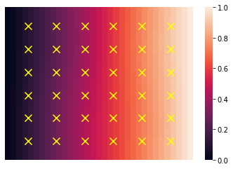
Figure 1: Eulerian observations of solution $u$

The quantity of interest for the problem is $K(x)$ with the coefficient $z$ being uniformly distributed.

$$K(x)=z\cos(2\pi x_{1})\sin(2\pi x_{2})+2.0,z\sim U[0,1]$$

We solve the above equation with the Finite Element method with uniformly spaced mesh. A $32\times 32$ mesh resolution is used in this experiment. We randomly generated 8000 samples with the FEM solver. The 8000 data are partitioned into 4000 training data, 2000 validation data, and 2000 test data to train a fully connected ReLU neural network with two hidden layers. Each layer of hidden layer has 512 nodes. The neural network is trained with Adam for 10000 epochs. We estimate the numerical error with $\mathbb{E}_{z\sim U[0,1]}(|u(z)-u_{ML}(z)|_{L2})$. To estimate the error, we use a high-fidelity resolution ($1024\times 1024$) solver to generate reference solutions and compute their L2 error. Gaussian Legendre quadrature methods are used to estimate the expectation value. We have the following estimator of the expected L2 error $\mathbf{E}(|u_{L=10}-u_{L=5}|_{L2})=5.576e^{-5}$ and $\mathbf{E}(|u_{L=10}-u_{ML}|_{L2})=3.132e^{-4}$. With the error, we have an estimate of $\epsilon=2.49$. We run three experiments with numerical solver based MCMC chain, ML model based MCMC chain and the proposed hybrid approach. The results of the average of 5 MCMC run are concluded in Table 1, from where we can see the results from the hybrid approach are comparable to the pure numerical solver based MCMC. A reference value computed with 32 points Gaussian Legendre quadrature and fine-meshed numerical solver $(1024\times 1024)$ is also included.

Method	Quadrature L=10	Quadrature L=5	Numerical	ML	Hybrid
Samples	N.A.	N.A.	100,000	100,000	100,000+4,000
QoI	0.3132	0.3128	0.3127	0.3061	0.3125

Table 1: Expectation of quantity of interest for the elliptic problem with uniform prior

7.2 Elliptic equation with log-normal prior

We consider the same Bayesian inverse problem with the forward model governed by the following elliptic equation shown in Section 7.1,

$$\begin{cases}\nabla\cdot(K(x)\nabla u(x))=\cos(2\pi x_{1})\sin(2\pi x_{2}),\\ u(x_{1}=0)=0,u(x_{1}=1)=1,\\ \frac{\partial u}{\partial x_{2}}(x_{2}=0)=\frac{\partial u}{\partial x_{2}}(x_{2}=1)=0.\end{cases}$$

Thirty-six equally distanced observations are captured from a random realization of the forward model with additional Gaussian noise $\delta$ with zero mean and variance $\sigma^{2}=0.2$. Now we consider the $K(x)$ of Gaussian random distribution. We sample the Gaussian random field from the following bi-laplacian Gaussian prior.

$$\mathcal{A}m=\begin{cases}\gamma\nabla\cdot(\Theta\nabla m)+\delta m&\text{ in }\Omega\\ (\Theta\nabla m)\cdot\boldsymbol{n}+\beta m&\text{ on }\partial\Omega\end{cases}$$

where we have $\gamma=0.1$, $\delta=0.5$ and $\beta=\sqrt{\gamma\delta}$. In the numerical experiment, we have the precision matrix $\mathcal{A}$ by discretizing the above equation and get $K(x)=\exp(m)$. We attach several examples of random field samples generated in this experiment in Figure 2.

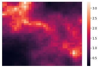
(a) sample 1

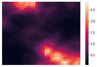
(b) sample 2

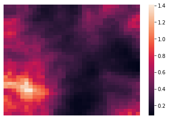
(c) sample 3

Figure 2: Samples from bi-laplacian random field

We solve the above equation with the Finite Element method with uniformly spaced mesh. A $32\times 32$ mesh resolution is used in this experiment. We randomly generated 8000 samples with the FEM solver. The 8000 data are partitioned into 4000 training data, 2000 validation data, and 2000 test data to train a convolutional neural network. The convolutional neural network consists of 3 encoding layer, 1 fully connected layer and 3 decoding layer. The neural network is trained with Adam for 10000 epochs. We estimate the numerical error with $\mathbb{E}_{m\sim N(0,\mathcal{A}^{-1})}(\frac{|u_{L=5}(m)-u_{ML}(m)|_{L2}}{|u_{L=5}(m)|_{L2}})$. In this experiment, we got an error of 0.102. With the error, we have an rough estimate of $\epsilon=1.179$. We run three experiments with numerical solver based MCMC chain, ML model based MCMC chain and the proposed hybrid approach. The results of the average of 5 MCMC run are concluded in Figure 3.

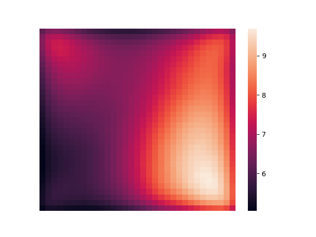
(a) numerical MCMC(100,000)

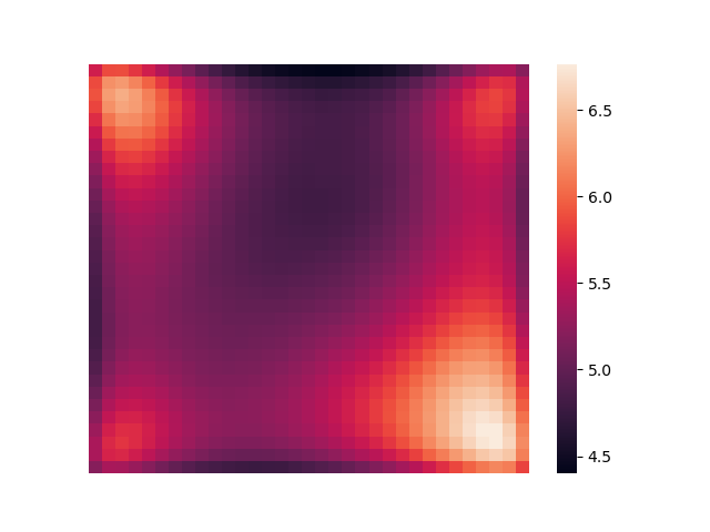
(b) ML MCMC (100,000)

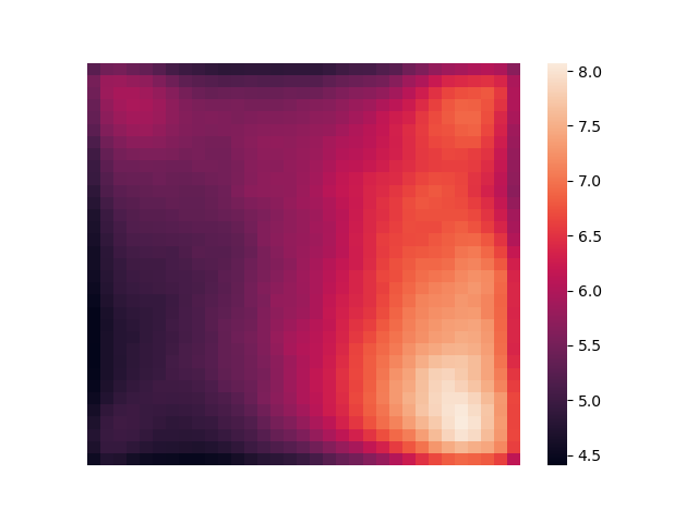
(c) Hybrid (100,000+1000)

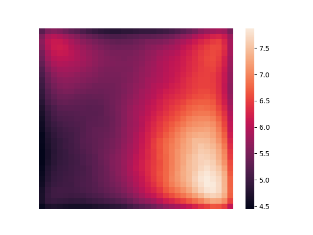
(d) Hybrid (100,000+4000)

Figure 3: Expected mean of $K(x)$ from 5 runs of MCMC

7.3 Nonlinear reaction-diffusion problem with Gaussian prior

We consider the Bayesian inverse problem with the forward model governed by the following reaction diffusion equation,

$$\begin{cases}\nabla\cdot(K(x)\nabla u(x))+u^{3}=0,\\ u(x_{1}=0)=0,u(x_{1}=1)=1,\\ \frac{\partial u}{\partial x_{2}}(x_{2}=0)=\frac{\partial u}{\partial x_{2}}(x_{2}=1)=0.\end{cases}$$

Thirty-six equally distanced observations are captured from a random realization of the forward model with additional Gaussian noise $\delta$ with zero mean and variance $\sigma^{2}=0.2$. Now we consider the $K(x)$ of Gaussian random distribution. We sample the Gaussian random field from the following bi-laplacian Gaussian prior.

$$\mathcal{A}m=\begin{cases}\gamma\nabla\cdot(\Theta\nabla m)+\delta m&\text{ in }\Omega\\ (\Theta\nabla m)\cdot\boldsymbol{n}+\beta m&\text{ on }\partial\Omega\end{cases}$$

where we have $\gamma=0.1$, $\delta=0.5$ and $\beta=\sqrt{\gamma\delta}$. In the numerical experiment, we have the precision matrix $\mathcal{A}$ by discretizing the above equation and get $K(x)=\exp(m)$. We solve the above equation with the Finite Element Method with uniformly spaced mesh. A $32\times 32$ mesh resolution is used in this experiment. We randomly generated 4000 samples with the FEM solver. The 4000 data are partitioned into 2000 training data, 1000 validation data, and 1000 test data to train a U-net neural network. The U-net consists of 3 layers, each with dimensions of $32\times 32$, $16\times 16$, and $8\times 8$. The neural network is trained with Adam for 10000 epochs. We run three experiments with a numerical solver based MCMC chain, ML model based MCMC chain and the proposed hybrid approach. The results of the average of 5 MCMC run are concluded in Fig 4. The results show a reduction in differences from maximum 1.2 to 0.5 with 2% of original numerical samples, to 0.35 with 10% of original numerical samples.

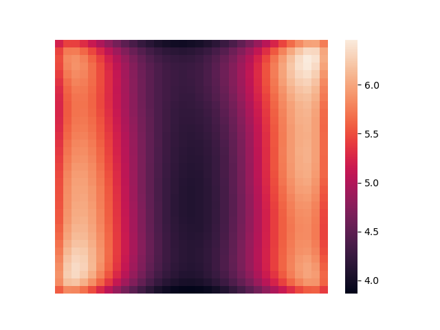
(a) numerical MCMC
(500,000)

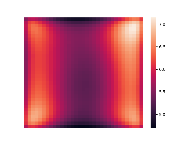
(b) ML MCMC
(500,000)

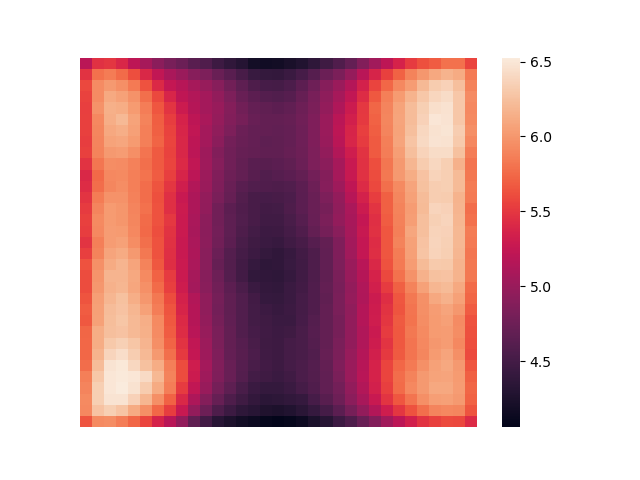
(c) Hybrid
(500,000+10,000)

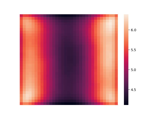
(d) Hybrid
(500,000+50,000)

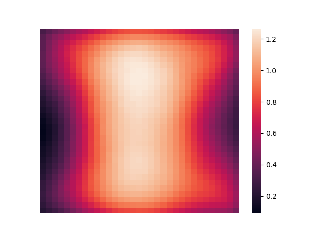
(e) ML MCMC
(500,000)

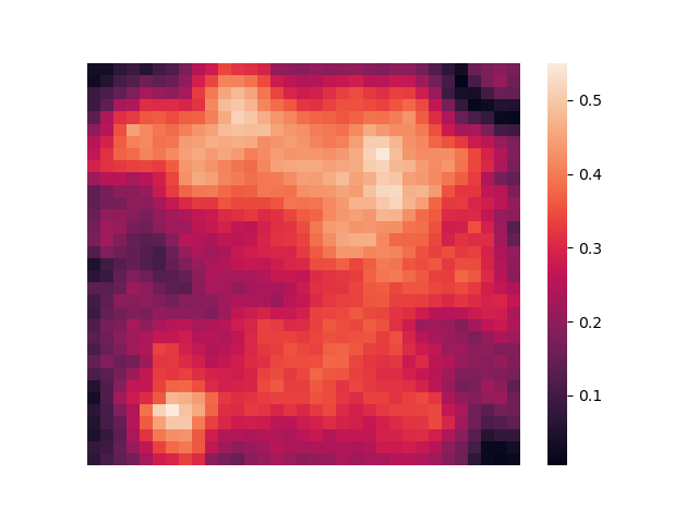
(f) hybrid MCMC
(500,000+10,000)

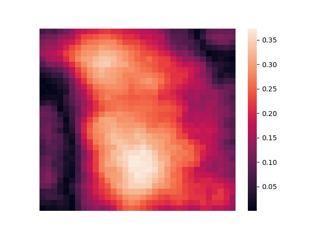
(g) hybrid MCMC
(500,000+10,000)

Figure 4: (a-d): Expected mean of $K(x)$ from 5 runs of MCMC, (e-g): the difference in comparison with the numerical MCMC chain

7.4 Two dimensional Navier Stokes Equation with Gaussian prior

We consider the Bayesian inverse problem with the forward model governed by the two dimensional Navier Stokes Equations in the vorticity form,

$$\begin{cases}\partial_{t}\omega(x,t)+u(x,t)\cdot\nabla\omega(x,t)-\nu\Delta\omega(x,t)=f,&\quad\text{for }x\in\mathbb{T}^{2},\\ \nabla\cdot u(x,t)=0,&\quad\text{for }x\in\mathbb{T}^{2},\\ \omega(x,0)=\omega_{0};\end{cases}$$

with the periodic boundary condition and the random forcing

$$f=0.1(\sin(2\pi(x_{1}+x_{2}))+\cos(2\pi(x_{1}+x_{2}))).$$ (18)

$\omega$ is the vorticity, $u$ is the velocity and $\nu=0.001$. 36 equal distanced observations are captured from a random realization of the forward model with additional Gaussian noise $\delta$ with zero mean and variance $\sigma^{2}=1$. Now we consider the $K(x)$ of Gaussian random distribution. We sample the Gaussian random field from the following bi-laplacian Gaussian prior with the following distribution: $\mathcal{N}(0,3^{\frac{3}{2}}(-\Delta+9I)^{-1})$. We solve the above equation with the pseudo-spectral method with Crank-Nicolson method. A $64\times 64$ resolution is used in this experiment. We randomly generated 4000 samples with the FEM solver. The 4000 data are partitioned into 2000 training data, 1000 validation data, and 1000 test data to train the Fouier Neural Operator (FNO) as described in [DBLP:conf/iclr/LiKALBSA21]. There are 12 modes for both height and width, 8 hidden channels and 4 layers for the FNO we used in this experiment. The neural network is trained for 10000 epochs. We run three experiments with a numerical solver based MCMC chain, ML model based MCMC chain and the proposed hybrid approach. The results of the average of 5 MCMC run are concluded in Figure 5. From Figure 5 we can see the posterior results from all three methods are the same. The posterior is close to the actual initial condition but different due to the no-linearly of the Navier Stokes equations.

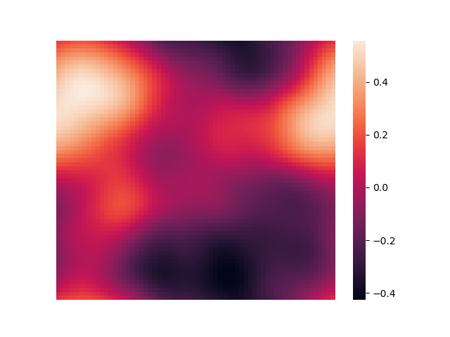
(a) Initial Condition

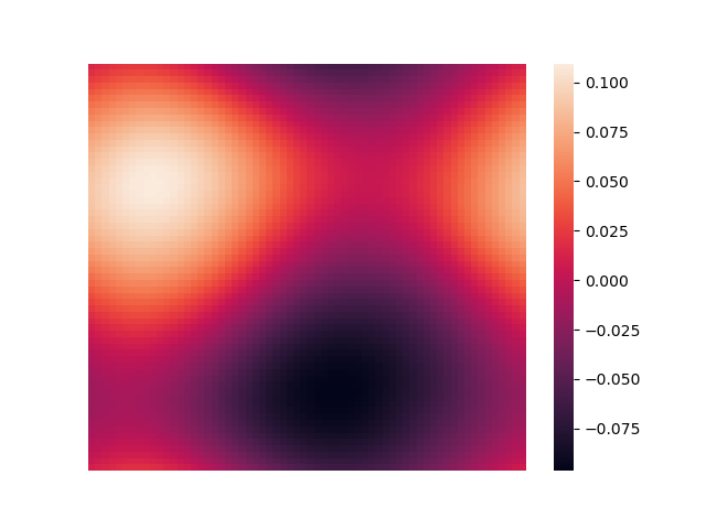
(b) Numerical MCMC
(10,000)

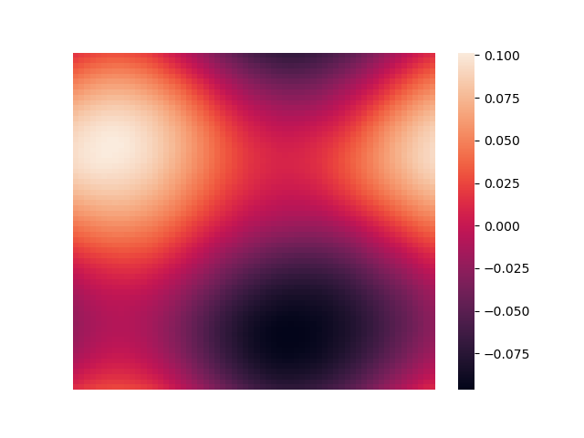
(c) AI MCMC
(10,000)

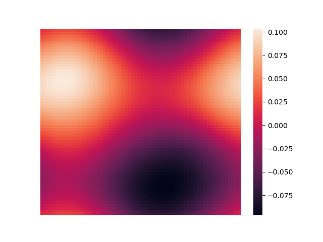
(d) Hybrid MCMC
(10,000+500)

Figure 5: Expected mean of $\omega_{0}$ from 5 runs of MCMC

Now we change the forcing from (18) to (19). Because the FNO model is not trained with this new forcing, the prediction of the AI model will not be accurate. Instead of regenerating training data and retraining the model, we use our hybrid method to correct the error of the AI model with the numerical model updated with the new forcing term.

$$f=0.2(\sin(2\pi(x_{1}+x_{2}))+\cos(2\pi(x_{1}+x_{2}))).$$ (19)

We run the same experiment and get the results shown in Figure 6. From the posterior expectation results, we can see the hybrid approach has a closer result to the numerical reference. The maximum difference is dropped from around 0.06 to 0.035. The L1 error is reduced from 0.030 to 0.013. We show that even with non-FEM-based numerical methods, e.g. spectral method used in this example, the hybrid approach still can accelerate the computation and improve accuracy.

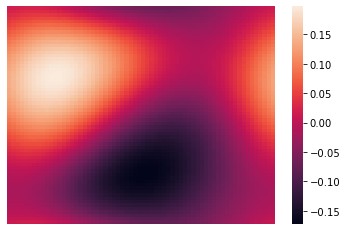
(a) numerical MCMC
(100,000)

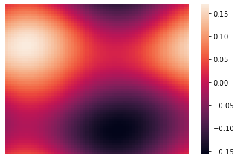
(b) ML MCMC
(100,000)

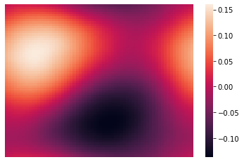
(c) Hybrid
(100,000+5,000)

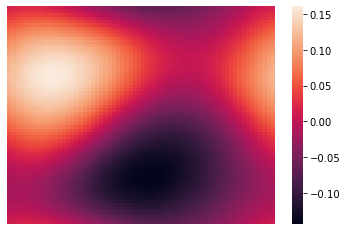
(d) Hybrid
(100,000+10,000)

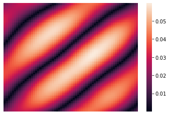
(e) ML MCMC
(100,000)

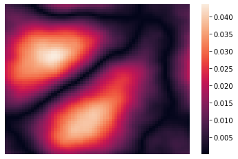
(f) hybrid MCMC
(100,000+5,000)

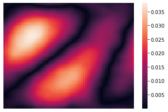
(g) hybrid MCMC
(100,000+10,000)

Figure 6: (a-d): Expected mean of $K(x)$ from 5 runs of MCMC, (e-g): the difference in comparison with the numerical MCMC chain

8 Conclusion

In this paper, we introduced a novel method to solve Bayesian inverse problems governed by PDE equations with a hybrid two-level MCMC where we took advantage of the AI surrogate model speed and the accuracy of numerical models. We have shown theoretically the potential to solve Bayesian inverse problems accurately with only a small number of numerical samples when the AI surrogate model error is small. Several numerical experiment results are included which are aligned with our claim.