Electrical operation of planar Ge hole spin qubits in an in-plane magnetic field

Abstract

Hole spin qubits in group-IV semiconductors, especially Ge and Si, are actively investigated as platforms for ultrafast electrical spin manipulation thanks to their strong spin-orbit coupling. Nevertheless, the theoretical understanding of spin dynamics in these systems is in the early stage of development, particularly for in-plane magnetic fields as used in the vast majority of experiments. In this work we present a comprehensive theory of spin physics in planar Ge hole quantum dots in an in-plane magnetic field, where the orbital terms play a dominant role in qubit physics, and provide a brief comparison with experimental measurements of the angular dependence of electrically driven spin resonance. We focus the theoretical analysis on electrical spin operation, phonon-induced relaxation, and the existence of coherence sweet spots. We find that the choice of magnetic field orientation makes a substantial difference for the properties of hole spin qubits. Furthermore, although the Schrieffer-Wolff approximation can describe electron dipole spin resonance (EDSR), it does not capture the fundamental spin dynamics underlying qubit coherence. Specifically, we find that: (i) EDSR for in-plane magnetic fields varies non-linearly with the field strength and weaker than for perpendicular magnetic fields; (ii) The EDSR Rabi frequency is maximized when the a.c. electric field is aligned parallel to the magnetic field, and vanishes when the two are perpendicular; (iii) The orbital magnetic field terms make the in-plane $g$-factor strongly anisotropic in a squeezed dot, in excellent agreement with experimental measurements; (iv) Focusing on random telegraph noise, we show that coherence sweet spots do not exist in an in-plane magnetic field, as the orbital magnetic field terms expose the qubit to all components of the defect electric field. These findings will provide a guideline for experiments to design ultrafast, highly coherent hole spin qubits in Ge.

I Introduction

Solid state spin qubits are prime candidates for scalable, highly coherent quantum computing platforms. Kane (1998); Loss and DiVincenzo (1998); Petta et al. (2005); Hanson et al. (2007); Hanson and Awschalom (2008); Zwanenburg et al. (2013); Chatterjee et al. (2021); Scappucci et al. (2021); Fang et al. (2023) Among these group IV materials such as Ge and Si stand out thanks to the absence of piezo-electric interaction with phonons Cardona and Peter (2005) and the possibility of isotopic purification, which eliminates the contact hyperfine coupling to the nuclear field,Itoh et al. (1993, 2003) with the maturity of semiconductor microfabrication as an added advantage. Recent years have witnessed a concerted push towards all-electrical qubit operation, since electric fields are easier to apply and localise than magnetic fields, and electrically operated qubit gates offer significant improvements in speed and power consumption as compared to magnetic gates. A series of theoretical predictionsBulaev and Loss (2007); Kloeffel et al. (2011, 2013); Chesi et al. (2014) as well as experimental leaps in growth techniques and sample quality Dobbie et al. (2012); Sammak et al. (2019); Lodari et al. (2019) have led to a surge in interest in spin-3/2 hole systems in group IV materials. The strong and multifaceted spin-orbit coupling experienced by holes, Cardona and Peter (2005); Winkler (2003); Winkler et al. (2008); Durnev et al. (2014); Marcellina et al. (2017) their anisotropic and tunable $g$-tensor, Danneau et al. (2006); Miserev and Sushkov (2017); Hung et al. (2017); Qvist and Danon (2022); Abadillo-Uriel et al. (2022) and the absence of a valley degree of freedom makes them ideal for electrical spin manipulation, with Ge offering the additional advantages of a small effective mass Terrazos et al. (2021) and ease of ohmic contact formation. Compared to electrons, the weaker hyperfine coupling for holesKeane et al. (2011); Chekhovich et al. (2011) due to the absence of the contact interaction significantly reduces the nuclear field contribution to spin decoherence, while the hole spin-3/2 is responsible for physics with no counterpart in electron systems, Culcer et al. (2006); Winkler et al. (2008); Liu et al. (2018); Abadillo-Uriel et al. (2018); Cullen et al. (2021) which may offer flexibility in future design strategies – for example magic angles have been predicted for acceptor qubits, Abadillo-Uriel et al. (2018) at which dipole-dipole entanglement can be switched off without switching off the electric dipole moments of single qubits.

Remarkable progress on hole spin qubits in several architectures has spanned more than a decade, with an overwhelming focus on Ge and Si.Chatterjee et al. (2021); Scappucci et al. (2021); Fang et al. (2023) Initial work focused on measuring hole spin states, Roddaro et al. (2008); Zwanenburg et al. (2009); Li et al. (2015); Liles et al. (2018) relaxation and dephasing times, Hu et al. (2012); Higginbotham et al. (2014); Vukušić et al. (2018) single spin electrical control, Pribiag et al. (2013) readout and control of the $g$-tensor Ares et al. (2013a, b); Brauns et al. (2016); Watzinger et al. (2016); Voisin et al. (2016); Srinivasan et al. (2016); Mizokuchi et al. (2018); Marcellina et al. (2018); Wei et al. (2020); Zhang et al. (2021); Liles et al. (2021) and of spin states in multiple dots, Li et al. (2015); Bohuslavskyi et al. (2016); Wang et al. (2016); van Der Heijden et al. (2018); Ezzouch et al. (2021) and achieving single-spin spin qubits. Maurand et al. (2016); Watzinger et al. (2018) In recent years the development of strained germanium in SiGe heterostructures Lodari et al. (2019, 2021); Terrazos et al. (2021) provided a low-disorder environment, which supported the development of single-hole qubits, Hendrickx et al. (2020a) singlet-triplet qubits, Jirovec et al. (2021) universal quantum logic, Hendrickx et al. (2020b) and a four-qubit germanium quantum processor.Hendrickx et al. (2021) Experiments have demonstrated ultrafast spin manipulation using the spin-orbit interaction Hendrickx et al. (2020b, a); Froning et al. (2021); Wang et al. (2022a) and EDSR Rabi oscillations as fast as $540$ MHz, Wang et al. (2022a) electrical control of the underlying spin-orbit coupling Gao et al. (2020); Liu et al. (2022) and charge sensing using a superconducting resonator, Ungerer et al. (2022) while relaxation times of up to 32 ms have been measured in Ge dots. Lawrie et al. (2020) Hole spins in Ge have been used as quantum simulators Wang et al. (2022b) and control of an array of 16 Ge hole dots has been demonstrated. Borsoi et al. (2022) The development of hybrid structures offers another path towards entanglement, with the demonstrations of superconductivity in planar Ge, Hendrickx et al. (2018); Aggarwal et al. (2021); Valentini et al. (2023) hole coupling to a superconducting resonator, Li et al. (2018) dipole coupling to a microwave resonator, Xu et al. (2020) charge sensing using a superconducting resonator Ungerer et al. (2022) and devices such as transistors and interferometers. Vigneau et al. (2019) Theoretically, the interplay of spin-orbit coupling and superconductivity in hybrid semiconductor-superconductor structures is only now being studied in the context of quantum computing. Lidal and Danon (2023)

Concomitantly, Si qubits have also registered remarkable recent progress, with coherence times of up to 10ms in Si:B acceptors Kobayashi et al. (2021) and the detection of sweet spots as a function of the top gate field in quantum dots, Piot et al. (2022) sweet spots having been the subject of a number of theoretical studies. Kloeffel et al. (2011); Salfi et al. (2016a, b); Abadillo-Uriel et al. (2018); Kloeffel et al. (2018); Marcellina et al. (2018); Terrazos et al. (2021); Wang et al. (2021); Bosco et al. (2021a); Bosco and Loss (2022); Wang et al. (2022c); Malkoc et al. (2022) Anisotropic exchange was also used to entangle two hole qubits, Geyer et al. (2022) hole coupling to a superconducting resonator has been demonstrated, Yu et al. (2022) and progress has been made towards higher-temperature operation with the observation of Coulomb diamonds up to 25K Shimatani et al. (2020) and single-qubit operation above 4K. Camenzind et al. (2022)

Despite experimental advances on many fronts, constructing an all-encompassing theory to describe hole physics in group-IV semiconductor quantum dots is challenging. In particular, owing to different effective masses and intrinsic spin-orbit gap in the valence band of these materials, the wide range of QD sizes as well as spin manipulation timescales exhibited in experiments render it difficult to provide a theory of spin qubits common to Si and Ge. In this work we will focus on Ge, which is somewhat more tractable analytically than Si, and describe electrical qubit operation in an in-plane magnetic field. This choice is motivated by the observation that experiments has overwhelmingly favoured in-plane magnetic fields, Watzinger et al. (2018); Hendrickx et al. (2020a) partly because a transverse magnetic field makes it easier to suppress hyperfine and cyclotron quantization effects, and partly in order to avoid the strong orbital coupling of the perpendicular field, which can cause a large diamagnetic shift and also affect tunnel rates. For spin-3/2 holes, in-plane magnetic fields are highly non-trivial, because the spin and orbital degrees of freedom are intertwined. The in-plane $g$-factor is very small, and in Ge most of it comes from the octupole interaction with the magnetic field.Winkler (2004) Whereas in-plane magnetic fields have been considered for realistic devices in recent theoretical studies, Ciocoiu et al. (2022); Wang et al. (2022c); Martinez et al. (2022) this has been largely from an engineering point of view, and the orbital effect of an in-plane magnetic field in planar quantum dots has largely been neglected, though they have been shown to play an important role in nanowires. Adelsberger et al. (2022) It has thus not been possible to date to construct a full picture of spin dynamics and electrical spin operation in planar Ge hole dots in an in-plane magnetic field. This has left several outstanding questions unanswered: What determines the speed of EDSR, as well as the relaxation time $T_{1}$? Is there an optimal magnetic field orientation for driving a spin-orbit qubit? Do coherence sweet spots exist when the magnetic field is in the plane?

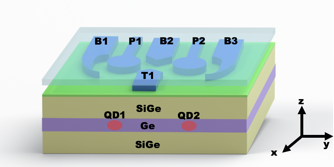
Figure 1: A prototype double quantum dot in a strained germanium hole system. The strained quantum well is grown epitaxially on a strain-relaxed SiGe layer. Gate B2 and T1 control the inter-dot tunneling. The growth direction is $\hat{\bm{z}}$.

In this work we seek to answer these questions. Our focus will be on gate-defined Ge quantum dots, with the parent 2DHG exhibiting very high mobilitySammak et al. (2019); Lodari et al. (2022), low percolation density,Lodari et al. (2021); Stehouwer et al. (2023), and a low effective mass of $m_{h}{=}\,0.05\,m_{e};$Hendrickx et al. (2018); Lodari et al. (2019), which all aid the formation of quantum dots. One reason for our choice of Ge is its band alignment, which makes it the only group IV material suitable for growing quantum wells. Another reason is pragmatic – it is easier to describe theoretically. This is because the spin-orbit splitting in Ge ($\Delta_{SO}{=}325\,\text{meV}$) is stronger than that in Si ($\Delta_{SO}{=}44\,\text{meV}$), resulting in a large separation of the spin-orbit/split-off (SO) band from the heavy- and light-hole subspaces. This ensures that the $4\!\times\!4$ Luttinger Hamiltonian formalism for spin-$3/2$ is adequate for the topmost Ge valence band, as opposed to Si where the Rashba mediated electrical control features both heavy hole-light hole (HH-LH) coupling contributions and heavy hole-split off (HH-SO) coupling contributions. Ge has a noticeable cubic-symmetry contribution to the Luttinger Hamiltonian. It is strong enough to enable electrical spin manipulation in planar dots, Terrazos et al. (2021); Wang et al. (2021) making Ge ideal for electrical spin operation, but not as strong as in Si, such that it can be treated perturbatively.

Figure. 1 provides a schematic of the device architecture for studying a planar germanium hole quantum dot qubit. In this paper we concentrate on developing the key formalisms for describing the spin physics of hole spin qubits in an in-plane magnetic field. To avoid unneccessary complexity, and to keep our results generally applicable, we avoid making the analysis overly device specific; therefore we do not consider effects of gate electrode induced non-uniform strain which can lead to a significant modification of the spin-orbit interaction;Liles et al. (2021); Corley-Wiciak et al. (2023) or Fowler-Norheim tunnelling of hole states through the SiGe barrier leading to charge accumulation at the interface between the semiconductor and the gate dielectric; or light-hole penetration through the SiGe barrier. Addressing these would require detailed finite element numerical simulation techniques on top of the theory developed here.

For an applied in-plane magnetic field operation of planar Ge hole QD, in the presence of uniaxial strain but neglecting shear strain, we show that: (i) EDSR is linear in the magnetic field with nonlinear corrections emerging at larger fields, and is driven by Rashba spin-orbit coupling rather than by the orbital magnetic field terms; the picture that emerges is that the orbital B terms give rise to the finite Zeeman splitting between the qubit energy levels, while the Rashba spin-orbit coupling gives rise to transitions between them. The EDSR Rabi frequency is a maximum when the electric field is parallel to the magnetic field, and vanishes when the two are perpendicular; it can be sizable despite the smallness of the in-plane $g$-factor, and has a non-monotonic dependence on $B$; (ii) The relaxation rate is due to bulk acoustic phonons and is proportional to $B^{3}$ in the leading power; Li et al. (2020) (iii) For a squeezed (elliptical) dot with an aspect ratio $L_{y}/L_{x}{=}\,2$ the spin-flip frequency is an order of magnitude faster than for a circular dot allowing Rabi time $\sim\!10$ ns with $\sim\!10^{5}$ operations within time $T_{1}$; (iv) For a squeezed dot, due to the effect of the magnetic field vector potential terms, the in-plane $g$-factor exhibits a strong anisotropy resulting in oscillatory behavior as the magnetic field is rotated in the plane of the dot, an observation supported by new experimental measurements shown in Sec. V of this paper; (v) Although extrema in the qubit Zeeman splitting as a function of the top gate voltage exist in the same way as for a perpendicular magnetic field,Wang et al. (2021) coherence sweet spots do not exist for in-plane magnetic fields for noise induced by charge defects in the plane of the quantum well. The physics underlying this process is associated with the orbital magnetic field terms and is not captured by the Schrieffer-Wolff approximation (although electrical qubit operation including EDSR can be described in a simplified Schrieffer-Wolff picture).

The outline of this paper is as follows. Section II lays down the foundation of the semi-analytical model of a Ge hole quantum dot qubit withing the framework of effective mass theory. Next we discuss the properties of circularly symmetric dots in Sec. III, including the qubit Zeeman splitting, EDSR, relaxation and dephasing. In Sec. IV we focus on elliptical dots and study their EDSR and coherence properties, while in Sec. V we discuss the consequences of $g$-factor anisotropy and compare our predictions with recent experimental results. We end with a summary and outlook in Sec. VI.

II Hamiltonian and model

The topmost valence band in Ge has orbital angular momentum $l{=}1$. When the hole spin $s{=}\frac{1}{2}$ is taken into account the resultant states at the $\mathbf{\Gamma}$-point are eigenstates of the total angular momentum $\mathbf{J}{=}(\mathbf{L}+\mathbf{S})$. The four-fold degenerate $j{=}\frac{3}{2}$ states are separated by the spin-orbit gap $\Delta_{0}$ from the $j{=}\frac{1}{2}$ two-fold degenerate split-off states. For Ge the spin-orbit gap $\Delta_{0}{=}325\,\text{meV}$, so the split-off band is safely disregarded in describing hole motion in the topmost valence bands. The $\left|\frac{3}{2}\right\rangle$ and $\left|-\frac{3}{2}\right\rangle$ states constitute the heavy-hole (HH) manifold while the $\left|\frac{1}{2}\right\rangle$ and $\left|-\frac{1}{2}\right\rangle$ states represent the light-hole (LH) manifold. The Luttinger Hamiltonian describes the hole motion in the topmost valence bands and has the following form in the $j{=}\frac{3}{2}$ basis $\left\{\left|\frac{3}{2}\right\rangle,\left|-\frac{3}{2}\right\rangle,\left|\frac{1}{2}\right\rangle,\left|-\frac{1}{2}\right\rangle\right\}$:

$$H_{LK}(k)=\begin{pmatrix}P^{\prime}+Q^{\prime}&0&L^{\prime}&M^{\prime}\\ 0&P^{\prime}+Q^{\prime}&M^{\prime*}&-L^{\prime*}\\ L^{\prime*}&M^{\prime}&P^{\prime}-Q^{\prime}&0\\ M^{\prime*}&-L^{\prime}&0&P^{\prime}-Q^{\prime}\\ \end{pmatrix}$$ (1)

where the matrix elements of the Luttinger Hamiltonian comprise the $k$-dependent part and strain-induced perturbations: $P^{\prime}{=}P(\mathbf{k})+P_{\varepsilon},\,Q^{\prime}{=}Q(\mathbf{k})+Q_{\varepsilon},\,L^{\prime}{=}L(\mathbf{k})+L_{\varepsilon},\,M^{\prime}{=}M(\mathbf{k})+M_{\varepsilon}$. The kinetic energy terms are $P\,{=}\frac{\hbar^{2}\gamma_{1}}{2m_{0}}(k_{x}^{2}+k_{y}^{2}+k_{z}^{2})$, $Q\,{=}\frac{\hbar^{2}\gamma_{2}}{2m_{0}}(k_{x}^{2}+k_{y}^{2}-2k_{z}^{2})$, $L\,{=}\frac{-\sqrt{3}\hbar^{2}\gamma_{3}}{m_{0}}(\{k_{x},k_{z}\}-i\{k_{y},k_{z}\})$ and $M\,{=}\frac{\sqrt{3}\hbar^{2}}{2m_{0}}\{-\gamma_{2}(k_{x}^{2}-k_{y}^{2})+2i\gamma_{3}\{k_{x},k_{y}\}\}$. The strain terms are: $P_{\varepsilon}{=}-a(\varepsilon_{xx}+\varepsilon_{yy}+\varepsilon_{zz})$, $Q_{\varepsilon}{=}-b(\varepsilon_{xx}+\varepsilon_{yy}-2\varepsilon_{zz})$, $L_{\varepsilon}{=}d(\varepsilon_{xz}-i\varepsilon_{yz})$ and $M_{\varepsilon}{=}\frac{\sqrt{3}}{2}b(\varepsilon_{xx}-\varepsilon_{yy})-d\varepsilon_{xy}$. Here $m_{0}$ is the bare electron mass while $\gamma_{1}$,$\gamma_{2}$ and $\gamma_{3}$ are Luttinger parameters. The constant $a{=}2\,\text{eV}$ is the hydrostatic deformation potential, $b{=}{-}2.16\,\text{eV}$ is the uniaxial deformation potential, and $d{=}{-}6.06\,\text{eV}$ accounts for the shear deformation potential. In most Ge/GeSi samples there is considerable strain in the quantum well, which significantly increases the splitting between light and heavy holes compared to silicon - here we take the compressive strain to be $0.6\%$.Sammak et al. (2019) The strain tensor components in the plane are: $\varepsilon_{xx}{=}\varepsilon_{yy}{=}-0.006$. The in-plane compressive strain elongates the out-of-plane lattice constant via $\varepsilon_{zz}{=}-2\frac{C_{12}}{C_{11}}\varepsilon_{xx}=0.004$; with $C_{12}{=}44$ GPa, $C_{11}{=}126$ GPa.Wortman and Evans (1965) We assume the off-diagonal shear elements of the strain tensor to be $\varepsilon_{ij|_{i\neq j}}{=}0$. The out-of-plane confinement is described by a one-dimensional infinite square well potential

$$V(z)=\begin{cases}\infty&z\in\left\{-\frac{L_{z}}{2},\frac{L_{z}}{2}\right\}\\ 0&\text{otherwise}\\ \end{cases}.$$ (2)

The coupling to the top-gate electric field, denoted by $F_{z}$, gives an additional term $eF_{z}z$ in the Hamiltonian. The in-plane confinement is modelled by a parabolic potential $V_{x,y}{=}\frac{1}{2}(\lambda_{x}^{2}x^{2}+\lambda_{y}^{2}y^{2})$, where $\lambda_{x},\,\lambda_{y}$ are determined by the dot dimensions $L_{x},\,L_{y}$ in the plane. The effective hole QD Hamiltonian is given by:

$$H_{0D}=H_{LK}(\mathbf{k})+eF_{z}z+V_{\text{conf}},$$ (3)

where $V_{\text{conf}}=V_{x,y}+V(z)$ is the total confinement potential. The Zeeman interaction is given by,

$$H_{Z}=-2\kappa\mu_{B}\mathbf{B}\cdot\mathbf{J}-2q\mu_{B}\mathbf{B}\cdot\mathcal{J},$$ (4)

where $\mathbf{J}=\{J_{x},\,J_{y},\,J_{z}\}$, $\mathcal{J}=\{J_{x}^{3},J_{y}^{3},J_{z}^{3}\}$; and $J_{x},\,J_{y},\,J_{z}$ are the $4{\times}4$ Pauli matrices. The $\mathcal{J}$-terms are vital in order to obtain the correct in-plane $g$-factor $\approx 0.25$.

In the presence of a magnetic field, the canonical momentum of holes in topmost valence band becomes $\mathbf{k}\rightarrow\left(\mathbf{k}+\frac{e\mathbf{A}}{\hbar}\right)$. The hole spin in a planar Ge quantum dot is then described by

$$H_{QD}=H_{LK}\!\!\left(\mathbf{k}+\frac{e\mathbf{A}}{\hbar}\right)+eF_{z}z+V_{\text{conf}}+H_{Z}.$$ (5)

The resultant modifications in $H_{LK}\left(\mathbf{k}+\frac{e\mathbf{A}}{\hbar}\right)$ lead to non-trivial contributions to the effective spin-orbit interaction in the HH and LH manifolds, as well as between them. To check the gauge invariance of our theoretical framework, we consistently diagonalise the effective quantum dot Hamiltonian using two different gauges:

1. $\mathbf{A}{=}-\frac{1}{2}B_{z}y\mathbf{\hat{e}_{x}}+\frac{1}{2}B_{z}x\mathbf{\hat{e}_{y}}+(B_{x}y-B_{y}x)\mathbf{\hat{e}_{z}}$.

2. The symmetric gauge: $\mathbf{A}\,{=}\,\frac{1}{2}\,\mathbf{B}\times\mathbf{r}\,{=}\,\frac{1}{2}(B_{y}z-B_{z}y)\,\mathbf{\hat{e}_{x}}+\frac{1}{2}(B_{z}x-B_{x}z)\,\mathbf{\hat{e}_{y}}+\frac{1}{2}(B_{x}y-B_{y}x)\,\mathbf{\hat{e}_{z}}$.

All calculations have been performed in both gauges, yielding consistent results.

The eigenstates of the hole QD can be expressed as linear combinations of states belonging to a basis in which the bare QD Hamiltonian is diagonal, i.e. $\left|\Psi_{QD}\right\rangle=\sum_{i}c_{i}\psi_{i}(x,y,z)\left|\phi_{j}\right\rangle$, where the bare Hamiltonian refers to $H_{QD}$ of Eq. 5 with its off-diagonal elements set to zero, following the practice of ${\bm{k}}\cdot{\bm{p}}$ theory, as well as the external magnetic field set to zero. We choose the spatial wave functions as $\psi(x,y,z){=}\psi_{n}(x)\,\psi_{m}(y)\,\psi_{l}(z)$, where the in-plane basis states are $\mathbf{1}$-D Harmonic oscillator states for $x$ and $y$ and the out-of-plane basis states are given by solutions of the infinite potential well:

$$\psi_{n}(x) = \frac{1}{\sqrt{2^{n}\,n!}}\frac{1}{\sqrt{L_{x}\sqrt{\pi}}}e^{-\frac{x^{2}}{2L_{x}^{2}}}H_{n}\!\!\left(\frac{x}{L_{x}}\right),\ x\in\{-\infty,\infty\}$$

$$\psi_{m}(y) = \frac{1}{\sqrt{2^{m}\,m!}}\frac{1}{\sqrt{L_{y}\sqrt{\pi}}}e^{-\frac{y^{2}}{2L_{y}^{2}}}H_{m}\!\!\left(\frac{y}{L_{y}}\right),\ y\in\{-\infty,\infty\}$$

$$\psi_{l}(z) = \begin{cases}\cos\!\left(\frac{(l+1)\pi z}{L_{z}}\right)&l\ \text{is even}\\ \sin\!\left(\frac{(l+1)\pi z}{L_{z}}\right)&l\ \text{is odd}\\ \end{cases}\ ,z\in\left\{-\frac{L_{z}}{2},\frac{L_{z}}{2}\right\}$$ (6)

The indices $n,m,l$ in Eqn. II can take integer values $0,1,2,3..$ etc. The hole spinors represent the $j{=}\frac{3}{2}$ spin states: $\left|\phi_{j}\right\rangle\in\left\{\left|\frac{3}{2}\right\rangle,\,\left|-\frac{3}{2}\right\rangle,\,\left|\frac{1}{2}\right\rangle,\,\left|-\frac{1}{2}\right\rangle\right\}$. When operated at low in-plane $\mathbf{B}$ we are in the $\omega_{c}\ll\omega_{0}$ limit, with $\omega_{c}$ the cyclotron frequency, so any effect of the in-plane magnetic field on the dot size are generally irrelevant (they are taken into account in our formalism). This means the Fock-Darwin solutions have a one-on-one analogy to the 2D Harmonic oscillator solutions in Eqn. II. The in-plane basis states $\Psi_{n}(x)\Psi_{m}(y)$ are ordered according to their energy $\propto(n+m+1)$. We find converging solutions to Eqn. 5 by considering $55$ in-plane basis states, i.e. $(n+m)\in[0,9]$; and $15$ out-of-plane $\Psi_{l}(z)$ basis states, i.e. $l\in[0,14]$. We note that the $(n+m)=0$ level has no degeneracy; but considering the degeneracies of $(n+m)=1,2....9$; the simulation spans $55$ in-plane levels. The numerical diagonalisation of the resultant $3300\times 3300$ Hamiltonian yields the energy levels of the hole quantum dot: $H_{QD}\left|\Psi_{QD}\right\rangle{=}\lambda_{E}\left|\Psi_{QD}\right\rangle$.

In the Schrieffer-Wolff approximation, which assumes the longitudinal confinement is much stronger than the in plane confinement, theoretical models show that the in-plane magnetic field gives rise to an effective spin-orbit coupling whose magnitude is proportional to $B$.Kloeffel et al. (2018); Wang et al. (2021) Recent experimental works have shown unambiguously that the $g$-factor of a 2D hole gas is a strong function of density,Marcellina et al. (2018); Akhgar et al. (2019), which can be captured by effective 2D theoretical modelsWinkler (2004); Miserev and Sushkov (2017); Miserev et al. (2017); Marcellina et al. (2017). Moreover, the effective spin-orbit interaction due to the orbital magnetic field terms has a highly non-trivial interplay with the Rashba spin-orbit interaction stemming from the top-gate potential.Winkler (2003, 2004); Miserev et al. (2017) For a hole QD in an in-plane $B$, as considered here, the orbital magnetic field terms also contribute to the spin dynamics. Nevertheless, this contribution, as the following sections make clear, cannot be captured by a naive Schrieffer-Wolff transformation, because the orbital magnetic field terms couple the in-plane and out-of-plane dynamics in a way that makes them inseparable: if one first reduces the 3D Hamiltonian to an effective $2\times 2$ Hamiltonian for a 2D hole gas, and then attempts to understand QD dynamics based on this effective 2D Hamiltonian (in analogy with electron systems) all the physics of the orbital magnetic field terms is lost. Hence a full 3D theoretical model is essential to understand the full spin dynamics of a hole quantum dot in an in-plane magnetic field. The model we present in this work can treat arbitrary quantum dot sizes, magnetic field strengths and orientations.

We comment briefly on the choice of spatial Ge basis functions. Variational analyses of the $z$-wave function incorporating the top gate potential have successfully described Ge hole QDs in Refs. Marcellina et al. (2017); Wang et al. (2021), but the variational model is hard to extend to a full 3D numerical analysis due to the complicated form of the variational excited states. For example, the Airy functionWang et al. (2022c); Li et al. (2020) provides the exact solution if the $z$ confinement is modelled as a triangular potential well but can yield a residual Rashba spin-orbit interaction at non-zero top gate potential ($F_{z}\!>\!0$), requiring a careful choice and implementation of boundary conditions. In the present paper we describe the $z$ confinement using an infinite square well augmented by a linear electrostatic potential that accounts for the top gate, and consider top gate fields up to 50MV/m (although values up to 100 MV/m can also be studied with this method). Ref. Wang et al., 2022c used a sophisticated model that incorporates Fowler-Nordheim tunnelling, which is beyond the scope of the present study, as explained below. We stress that the range of $F_{z}$ is at the lower end of what we consider here (up to 2.5 MV/m), and thus our studies can be regarded as complementary.

III Circular Quantum dot

Qubit Zeeman splitting.

We solve the full 3D Hamiltonian in an external magnetic field along $x$ for a QD with following dimensions: $L_{x}{=}50\,\text{nm}$,$L_{y}{=}50\,\text{nm}$,$L_{z}{=}11\,\text{nm}$.

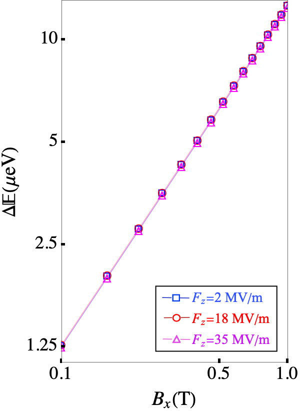
(a)

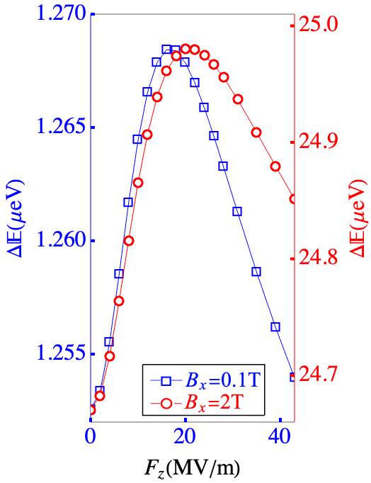
(b)

Figure 2: Qubit Zeeman splitting of hole spin-qubit in $B_{\parallel}$. a) Variation in the qubit Larmor frequency $\Delta\mathbb{E}$ ($\mu\text{eV}$) with the in-plane magnetic field $B_{x}$(T). The Zeeman splitting shows a monotonic linear trend with $B_{x}$ at $F_{z}{=}2\,\text{MV/m}$, $F_{z}{=}18\,\text{MV/m}$ and $F_{z}{=}35\,\text{MV/m}$ top-gate potentials respectively; with in-plane $g_{\parallel}{\sim}\,0.22$. No significant difference occurs in the qubit Larmor frequency for different top gate field. b) The in-plane $g$-factor exhibits an extremum as a function of the top gate at $F_{z}{=}18\,\text{MV/m}$ and $F_{z}{=}21\,\text{MV/m}$, respectively for $B_{x}{=}0.1\text{T}$ and $B_{x}{=}2\text{T}$.

The ground state is given by $\left|\Psi_{QD}\right\rangle=\sum_{i}c_{i}\psi_{i}(x,y,z)\left|\phi_{j}\right\rangle$. We evaluate the QD ground state and first excited state, labelling them as state $\left|\mathbb{0}\right\rangle$ with eigenenergy $\mathbb{E_{0}}$ and $\left|\mathbb{1}\right\rangle$ with eigenenergy $\mathbb{E_{1}}$ repectively. The ground state and the first excited state are of heavy hole-type with admixtures due to heavy hole-light hole coupling, and split by an amount $\Delta\mathbb{E}{=}\mathbb{E_{1}}-\mathbb{E_{0}}$, which we refer to as the qubit Larmor frequency, while continuing to express it in units of energy. The HH-LH splitting $\Delta_{LH}\sim 60\text{meV}$ is governed by the $z$-energy bands in the quasi 2D dot limit , so that many in-plane (quantum dot) levels are contained between any two out-of-plane (quantum well) levels. This allows us to write $\left|\mathbb{0}\right\rangle{=}(c_{1}\left|0,0,0,\frac{3}{2}\right\rangle+\text{admixtures})$ and $\left|\mathbb{1}\right\rangle{=}(c_{1}^{\prime}\left|0,0,0,-\frac{3}{2}\right\rangle+\text{admixtures})$, where the four indices denote $n,\,m,\,l,\,J_{z}$. When plotted against the top-gate voltage, the qubit Larmor frequency exhibits an extremum as a function of $F_{z}$.Wang et al. (2021) The in-plane magnetic field gives rise to a finite Zeeman splitting, which shows a linear trend with $B_{x}$ (figure 2a). The extrema in the qubit Larmor frequency as a function of $F_{z}$ in an in-plane $\mathbf{B}$ are explained by the same mechanism as for out-of-plane magnetic field operation (Figure 2b). At small values of $F_{z}$ the matrix elements connecting the HH and LH states, which give rise to Rashba spin-orbit coupling, increase linearly with the gate field, while the change in the HH-LH splitting is negligible. At large values of $F_{z}$ the increase in the HH-LH splitting outweighs all other effects and the Rashba spin-orbit coupling decreases as a function of $F_{z}$. These competing effects give rise to an extremum in the qubit Larmor frequency at a certain value of the top gate electric field, where the qubit is insensitive to $z$-electric field fluctuations. The qubit Zeeman splitting is linear in $\mathbf{B}$, $\Delta\mathbb{E}{=}g_{\parallel}\mu_{B}B_{x}$, where the effective in-plane $g$-factor ranges between $0.215-0.219$, expected to be much smaller than out-of-plane $g$-factor; $g_{\parallel}\ll g_{\perp}$.

EDSR.

An alternating electric field $\tilde{\mathbf{E}}(t)$ can induce spin-flip transition between the qubit states $\left|\mathbb{0}\right\rangle$ and $\left|\mathbb{1}\right\rangle$ via electron dipole spin resonance (EDSR) when the frequency of the ac electric field matches the Zeeman splitting of the hole spin qubit, $\Delta\mathbb{E}{=}h\nu$.

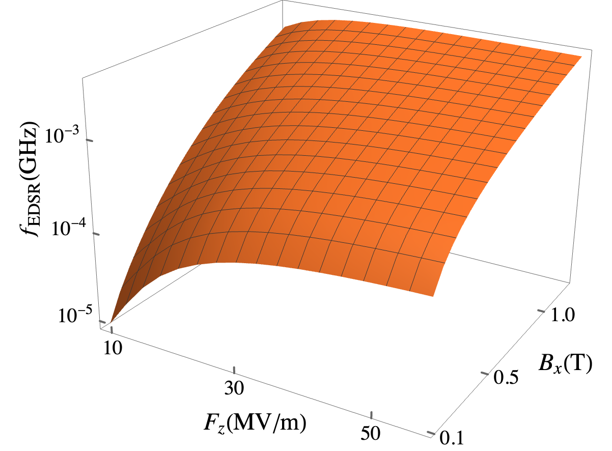
5

(a)

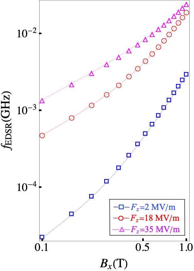
(b)

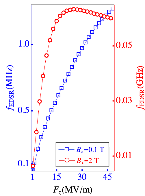
(c)

Figure 3: Electric dipole spin resonance of hole qubit in $B_{\parallel}.$ a) Dependence of the EDSR Rabi frequency $f_{\text{EDSR}}$(GHz) on the top gate field $F_{z}$(MV/m) and in-plane magnetic field $B_{x}$(T). The strength of the in-plane EDSR driving ac electric field is $E_{0}=10\,\text{kV/m}$. The $z$-axis representing $f_{\text{EDSR}}$ in the $3$D plot is logarithmic. b) Variation of $f_{\text{EDSR}}$ with $B_{x}$ showing a non-monotonic dependence on the applied $B$-field as: $f_{\text{EDSR}}{=}a_{f}B_{x}{+}b_{f}B_{x}^{2}{+}c_{f}B_{x}^{3}$. The points on the plot signify results from the numerical calculation while the fitting is denoted by the dashed lines. At $F_{z}{=}2\,\text{MV/m}$ the fitting parameters are $a_{f}=0.0002,\,b_{f}=0.00002,\,c_{f}=0.003$; at $F_{z}{=}18\,\text{MV/m}$ they are $a_{f}=0.005,\,b_{f}=0.00006,\,c_{f}=0.01$ and at $F_{z}{=}35\,\text{MV/m}$ top-gate potential the fitting parameters are $a_{f}=0.01,\,b_{f}=0.00004,\,c_{f}=0.01$. c) The Rabi frequency exhibits maxima as a function of the top gate at $F_{z}{=}18\,\text{MV/m}$ only for higher magnetic field ($B_{x}{=}2\text{T}$), over the range of top-gate potentials used in this study.

The EDSR Rabi frequency is calculated as the matrix element of the ac field between the qubit ground state (GS) and excited state (ES):

$$f_{\text{EDSR}}=\left\langle\mathbb{0}\left|e\tilde{\mathbf{E}}(t)\cdot\mathbf{r}\right|\mathbb{1}\right\rangle$$ (7)

Here we will focus on the scenario in which the alternating electric field is in the plane. In the 3D model, the effective interaction between the qubit GS and ES wavefunctions lies in the LH admixture to $\left|\pm\frac{3}{2}\right\rangle$ HH states. The admixture is the results of the two primary spin-orbit interactions in the system: structure inversion asymmetry (SIA) due to the top-gate potential $F_{z}$ gives rise to the first Rashba term, which stems primarily from HH-LH coupling. The second contribution to the spin-orbit interaction comes from the orbital terms due to the in-plane magnetic field $\mathbf{B}$. As $\mathbf{B}$ is ramped up, the magnitude of this latter contribution increases. For an applied oscillatory electric field of strength $E_{0}{=}10\text{kV/m}$, figure 3a presents the spin-flip Rabi frequency variation with the top gate field and applied $B_{x}$, with the key features of the EDSR frequency exhibiting a maximum at a certain value of $F_{z}$, as well as a nonlinear dependence of $f_{\text{EDSR}}$ on $B_{x}$. In figure 3b, $f_{\text{EDSR}}$ shows a non-linear variation as a function of the in-plane magnetic field. The best fit corresponds to $f_{\text{EDSR}}{=}a_{f}B_{x}{+}b_{f}B_{x}^{2}{+}c_{f}B_{x}^{3}$ at a constant top gate field. At $B_{x}{=}0.1\,\text{T}$ the Rabi frequency increases slowly with the top gate field. On the other hand at ($B_{x}{=}2\,\text{T}$) the Rabi frequency increases more rapidly with $F_{z}$, and the maximum shifts towards lower values of $F_{z}$ (Fig. 3c). We find the EDSR rate is a maximum when the electric field is parallel to the magnetic field, and vanishes when the two are perpendicular.

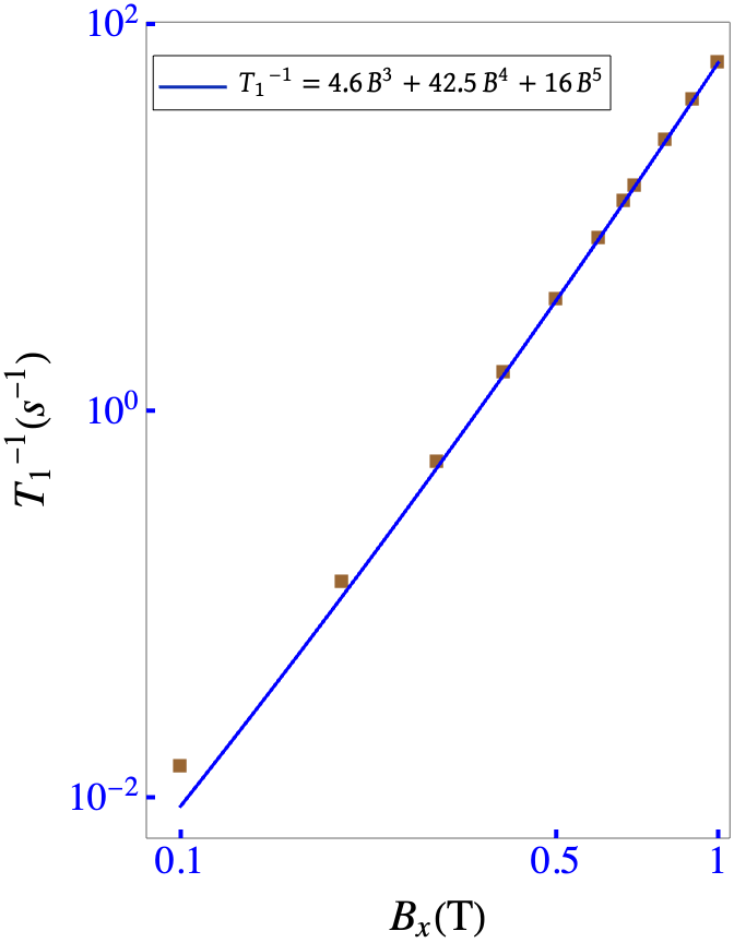
(a)

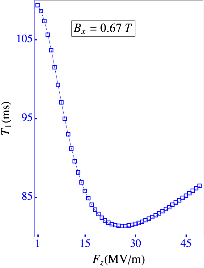
(b)

Figure 4: Phonon induced hole spin-qubit relaxation for $B_{\parallel}$ operation. a) Relaxation rate $T_{1}^{-1}\,(\text{s}^{-1})$ vs. applied magnetic field $B_{x}$ (T) at the top-gate field of $F_{z}{=}18\,\text{MV/m}$. The B-dependence of the relaxation rate has been fitted using the fitting parameters shown in the top inbox. b) The relaxation rate $T_{1}^{-1}$ vs. the top gate field $F_{z}$ (MV/m) for $B_{x}{=}0.67\,\text{T}$.

The nonlinearity in $F_{z}$ in figure 3c reflects the quadrupole Rashba spin-orbit coupling unique to spin-3/2 systems,Winkler (2004) having no counterpart in electron spin qubits. Hole qubits in Ge quantum dots can exhibit fast EDSR of the order of $\sim\!100\,\text{ns}$, despite the fact that the in-plane $g$-factor is two orders of magnitude smaller than the out-of-plane $g$-factor. The linear term in $B_{x}$ in the Rabi frequency (figure 3b) stems from the Zeeman terms cubic in angular momentum $\propto q$ in Eq. 4. To see this one can write an effective $2{\times}2$ qubit Hamiltonian using the Schrieffer-Wolff (SW) transformation up to third order in small quantities:

$$H_{\text{eff}}^{2{\times}2}=H_{0}+H_{SO}+g_{\parallel}\mu_{B}B_{x}^{3}\sigma_{x}+V(x,y)+eE_{x}(t)x$$ (8)

Here $H_{0}\!(\mathbf{k}{\rightarrow}(\mathbf{k}{+}e\mathbf{A}/\hbar)){=}[\mathcal{A}k^{2}\!-\!\mathcal{B}k^{4}\!-\!D(k_{+}^{2}\!-\!k_{-}^{2})^{2}]\!I_{2{\times}2}$ is the kinetic energy including a correction $\propto k^{4}$,Winkler (2004) and the $D$ term represents warping of the energy contours.Marcellina et al. (2017) The spin-orbit Hamiltonian $H_{SO}$ comprises two important $k$-cubic Rashba terms induced by the top gate field, a spherical term $\propto\alpha_{R2}$ and a cubic-symmetric correction $\propto\alpha_{R3}$. The next three terms represent the Zeeman splitting, confinement energies and the ac electric potential along the $x$-direction, respectively. Starting from this effective Hamiltonian and projecting it onto the in-plane states, one may apply the SW approximation again to obtain an effective $2\times 2$ qubit Hamiltonian, in which the EDSR driving term appears on the off-diagonal. Reading off the EDSR Rabi frequency we find $f_{\text{EDSR}}{\propto}B_{x}$ to leading order, while the next order in the expansion gives $f_{\text{EDSR}}\propto B_{x}^{3}$ (Appendix. B).

The significant quadratic $B_{x}^{2}$ dependence of the EDSR Rabi frequency at large $F_{z}$ (Fig. 3c) is a signature of the orbital magnetic field terms. One can determine possible paths connecting the lowest energy $\left|\mathbb{0}\right\rangle{\leftrightarrow}\left|\mathbb{1}\right\rangle$ HH-qubit states, mainly composed of $\left|0,0,0,\frac{3}{2}\right\rangle$ and $\left|0,0,0,-\frac{3}{2}\right\rangle$ with admixtures, respectively. Choosing the symmetric gauge for $\mathbf{B}{=}(B_{x},0,0)$, the magnetic field induces the following transitions in the Luttinger-Kohn picture: $\left\{\left|\frac{3}{2}\right\rangle\!{\xrightarrow{B_{x}}}\!\left|\frac{1}{2}\right\rangle,\,\left|-\frac{1}{2}\right\rangle\!{\xrightarrow{B_{x}}}\!\left|-\frac{3}{2}\right\rangle\right\}$. The gate potential gives $\left\{n_{z}{\xrightarrow{eF_{z}z}}n_{z}{\pm}1\right\}$ which is spin conserving. The Luttinger terms $L(\mathbf{k}),\,M(\mathbf{k})$ couple HH and LH states e.g. $\left\{\left|n_{x},n_{y},n_{z},\frac{3}{2}\right\rangle\!{\xrightarrow[L(\mathbf{k})]{k_{x}k_{z}}}\!\left|n_{x}\pm 1,n_{y},n_{z}\pm 1,\frac{3}{2}\right\rangle\right\}$. We consider the complete SO picture in the Ge hole QD following eqn. 5 to sketch a few example paths as follows:

• $\left|0,0,0,\frac{3}{2}\right\rangle\!{\xrightarrow[L]{B_{x}}}\!\left|0,0,0,\frac{1}{2}\right\rangle\!{\xrightarrow[L]{k_{y}k_{z}}}\!\left|0,1,1,\frac{3}{2}\right\rangle\!{\xrightarrow[M]{k_{x}k_{y}}}$
   $\left|1,2,1,-\frac{1}{2}\right\rangle\!{\xrightarrow{eF_{z}z}}\!\left|1,2,0,-\frac{1}{2}\right\rangle\!{\xrightarrow{eE_{x}x}}\!\left|0,2,0,-\frac{1}{2}\right\rangle\!{\xrightarrow[J\rightarrow J]{k_{y}^{2}}}$
   $\left|0,0,0,-\frac{1}{2}\right\rangle\!{\xrightarrow[L]{B_{x}}}\!\left|0,0,0,-\frac{3}{2}\right\rangle$.

• $\left|0,0,0,\frac{3}{2}\right\rangle\!{\xrightarrow[L]{k_{y}k_{z}}}\!\left|0,1,1,\frac{1}{2}\right\rangle\!{\xrightarrow{eE_{x}x}}\!\left|1,1,1,\frac{1}{2}\right\rangle\!{\xrightarrow[J\rightarrow J]{B_{x}yk_{z}}}$
   $\left|1,0,2,\frac{1}{2}\right\rangle\!{\xrightarrow{(eF_{z}z)^{2}}}\!\left|1,0,0,\frac{1}{2}\right\rangle\!{\xrightarrow[M]{k_{x}k_{y}}}\!\left|0,1,0,-\frac{3}{2}\right\rangle\!{\xrightarrow[J\rightarrow J]{B_{x}yk_{z}}}$
   $\left|0,0,1,-\frac{3}{2}\right\rangle\!{\xrightarrow{eF_{z}z}}\!\left|0,0,0,-\frac{3}{2}\right\rangle$.

These paths explain the quadratic $B_{x}^{2}$ dependence at large $F_{z}$ in the presence of the ac electric field.

Phonon mediated Relaxation.

The relaxation mechanism in Ge hole QD qubits is well explained by acoustic phonon coupling to the hole spins through the valence band deformation potential $\mathcal{D}_{i,j}$ of Ge. There are no piezo-electric phonons in Ge, but the hole spin interacts with the thermal bath of the bulk phonons via the hole-phonon Hamiltonian $H_{h-ph}$, where $\alpha\in\{l,t,w\}$ denotes the polarization directions of the phonon and $\mathbf{q}$ is the phonon wave vector. We write $H_{h-ph}{=}\sum_{i,j}\mathcal{D}_{i,j}\varepsilon^{\alpha}_{i,j}(\bm{r})$ with $\varepsilon^{\alpha}_{i,j}(\bm{r})=\sum_{q}\frac{i}{2}\sqrt{\frac{\hbar}{2\rho NV\omega_{\mathbf{q},\alpha}}}\left(q_{i}\hat{c}_{j}+q_{j}\hat{c}_{i}\right)e^{i\bm{q}\cdot\bm{r}}\sqrt{N_{q}^{\alpha}+1}$. The relaxation rate $1/T_{1}$ is written as:

$$\frac{1}{T_{1}}=\frac{2\pi}{\hbar}\sum_{\alpha,\mathbf{q}}\left|\left\langle\mathbb{0}\right|H_{h-ph}\left|\mathbb{1}\right\rangle_{\alpha}\right|^{2}\delta\left(\Delta\mathbb{E}-\hbar\omega_{\alpha,\mathbf{q}}\right)$$ (9)

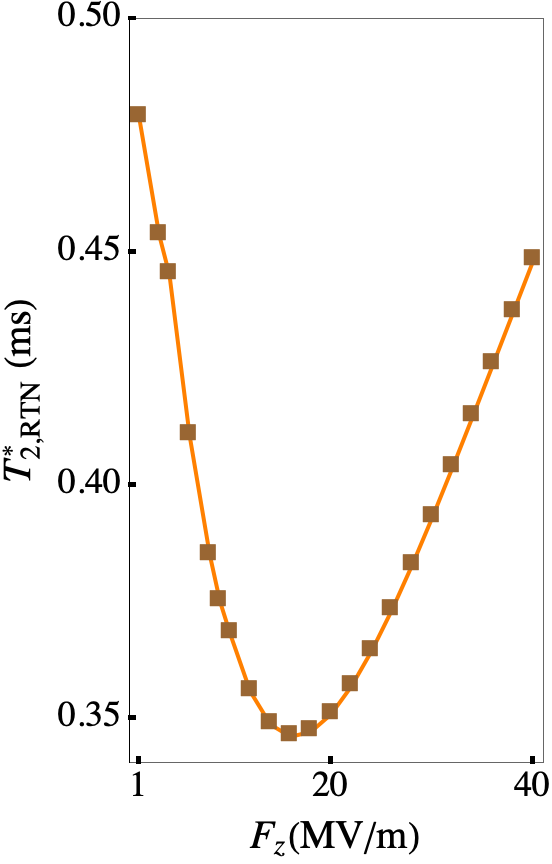
(a)

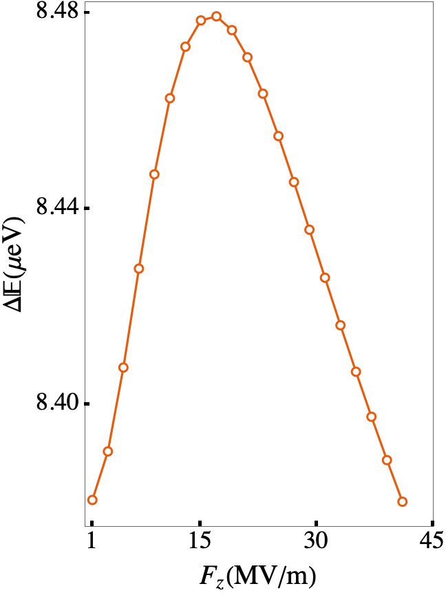
(b)

Figure 5: Qubit dephasing in an in-plane magnetic field: a) Variation of qubit dephasing time $T_{2,\text{RTN}}^{*}$ (ms) due to random telegraph noise (RTN) from a nearby in-plane single charge defect 200 nm away from the qubit w.r.t. top gate field $F_{z}$ (MV/m). b) Qubit Zeeman splitting $\Delta E\,(\mu\text{eV})$ vs. applied top-gate field $F_{z}$ (MV/m). The applied magnetic field is in the plane with the magnitude $B_{x}{=}0.67\,\text{T}$. The dephasing time reaches a minimum at $F_{z}{=}18\,\text{MV/m}$.

We calculate the relaxation rate using our semi-analytical 3D QD model by computing in real space the overlap integral $\left\langle\mathbb{0}\right|H_{h-ph}\left|\mathbb{1}\right\rangle_{\alpha}$ due to position-dependent local strain, followed by the scattering integral in the phonon wave vector $q$-space for a specific polarization direction. The full analytical integrations and dipole approximation calculations are detailed in Appendix. C. Figure 4a shows the nonlinear variation of the relaxation rate $T_{1}^{-1}$ w.r.t. the external magnetic field $B_{x}$, with $B^{3}$, $B^{4}$ and $B^{5}$ terms present in the fitting obtained from the full 3D numerical model. While the $B^{3}$ and $B^{5}$ dependence are explained from the first two terms in the dipole approximation, the $B^{4}$ term is understood from the orbital $B$-admixture. A minimum relaxation time $T_{1}\sim 80\,\text{ms}$ at an in-plane magnetic field $B_{x}{=}0.67\,\text{T}$ is obtained. This result from the theory compares well with a single hole relaxation time measurement in Ge of over 30 ms and a five-hole relaxation time of approximately 1 ms by Lawrie et al.Lawrie et al. (2020) The magnetic field in the experimental setupHendrickx et al. (2020a); Lawrie et al. (2020) is $B{=}0.67\,\text{T}$, as also used in Fig. 4a. There exists a minimum in $T_{1}$ in the range of $F_{z}$ considered here for $B_{x}{=}0.67\,\text{T}$ (figure 4b). At this minimum the Rabi ratio $T_{1}/T_{\pi}{\approx}2\times 10^{5}$, where $T_{\pi}$ is the time required for an EDSR $\pi$-rotation, demonstrating that fast Rabi oscillations can be achieved without sacrificing $T_{1}$.

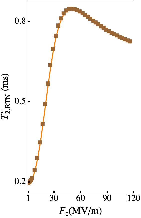
(a)

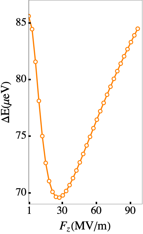
(b)

Figure 6: Qubit dephasing in an out-of-plane magnetic field: a) Variation of qubit dephasing time $T_{2,\text{RTN}}^{*}$ (ms) due to random telegraph noise (RTN) from a nearby in-plane single charge defect 200 nm away from the qubit w.r.t. top gate field $F_{z}$ (MV/m). b) Qubit Zeeman splitting $\Delta E\,(\mu\text{eV})$ vs. applied top-gate field $F_{z}$ (MV/m). The applied magnetic field is in the plane with the magnitude $B_{x}{=}0.1\,\text{T}$. In this case, the dephasing time exhibits a maximum in top-gate field.

Random Telegraph Noise (RTN) Dephasing.

The large spin-orbit coupling exposes the hole spin qubit to charge noise. The dephasing time $T^{*}_{2,\text{RTN}}$ is evaluated from the fluctuation in the qubit energy gap, denoted by $\delta\omega$, caused by the screened potential $U_{s}(\bm{r})$ of a nearby single charge defect in the 2DHG.Maman et al. (2020); Culcer et al. (2009); Ramon and Cywiński (2022); Roszak et al. (2019); Malkoc et al. (2022) The mathematical formulation of $U_{s}(\bm{r})$ is given in Appendix. D. The matrix elements $\left\langle n,m,l|U_{s}(\bm{r})|n^{\prime},m^{\prime},l^{\prime}\right\rangle$ are added to the full Hamiltonian, and the $3300\times 3300$ matrix is diagonalised to evaluate the qubit energy splitting in the presence of the charge defect as $\Delta\mathbb{E}+\delta\omega$. The dephasing rate is:

$$\left(T^{*}_{2,\text{RTN}}\right)^{-1}{=}\frac{(\delta\omega)^{2}\tau}{2\hbar^{2}}$$ (10)

where the defect switching time is taken as $\tau{=}10^{3}\,t_{Rabi}$. This picture assumes the most significant contribution to RTN comes from charge defects away from the top gate, close to the qubit plane; hence we consider a single charge defect in the qubit plane situated $200$ nm away from the center of the qubit. Fluctuating single charge defects right above the qubit will be screened by the presence of the top-gate, where the image charge changes the interaction to a much weaker dipole interaction. In contrast fluctuating charges in the plane of the quantum well are less effectively screened by surface gates, and may be the dominant source of charge noise. Culcer and Zimmerman (2013)

It is evident that for hole qubit in an in-plane magnetic field, the dephasing time $T_{2,RTN}^{*}$ actually decreases as a function of the top gate electric field $F_{z}$, and reaches a minimum at a certain value of this field (Fig. 5a), in other words, a coherence hot spot. The location of this dephasing time hotspot is closely related to the extremum in the qubit Zeeman splitting (Fig. 5b). This behaviour is in sharp contrast to hole spin qubits in a perpendicular magnetic field, where the qubit exhibits a sweet spot at a certain value of the top gate field (Fig. 6a), at which its sensitivity to noise vanishes to leading order in the noise strength, and dephasing time $T_{2,RTN}^{*}$ reaches a maximum. The location of the sweet spot in $F_{z}$ for out-of-plane qubit operation is closely related to an extremum in the qubit Zeeman splitting (Fig. 6b).

$B_{\perp}$ vs. $B_{\parallel}$ coherent qubit operation.

In the context of qubit coherence one must distinguish between extrema in the qubit Zeeman splitting and actual sweet spots in the coherence time. It is important to recall that in a spin qubit the dephasing time $T_{2}^{*}$ depends on the magnitude of the magnetic field. This follows from time-reversal symmetry considerations, since the combination of charge noise and spin-orbit coupling cannot give rise to an energy difference between qubit states that form a Kramers doublet. The magnetic field dependence involves both the Zeeman terms and the orbital vector potential terms, a fact that is responsible for the main difference between in-plane and out-of-plane magnetic fields with regard to qubit dynamics: the make up of the ground and first excited states is very different when the magnetic field is in the plane and when it is out of the plane.

For an out of plane magnetic field the hole $g$-factor is large, having a textbook value of 20.4 for Ge.Winkler (2003); Lu et al. (2017) With the magnetic field out of the plane one can understand the physics qualitatively by considering an approximate decomposition of in-plane and out-of-plane dynamics by means of a Schrieffer-Wolff transformation Wang et al. (2021) The picture that emerges is that the top gate electric field primarily affects spin dynamics in the plane by enabling a Rashba term. In a quantum dot this Rashba term is responsible for a renormalization of the $g$-factor. In other words, one can think of the magnetic field terms as providing the qubit Zeeman splitting, and the Rashba spin-orbit terms as renormalizing this Zeeman splitting. Background charge fluctuations generating an electric field perpendicular to the plane are the biggest danger for this qubit, because they directly affect the Rashba interaction and through it the $g$-factor, generating pure dephasing. A more detailed analysis of hole spin qubit in $B_{\perp}$ Wang et al. (2021) reveals that in-plane charge fluctuations do not produce pure dephasing to leading order. Hence for $B_{\perp}$ operation, when the qubit Zeeman splitting is at an extremum with respect to the top gate electric field (Fig. 6b), the qubit is protected against noise and one also observes a sweet spot in $T_{2}^{*}$ in the vicinity of this point (Fig. 6a).

On the other hand, for hole spin qubit in $B_{\parallel}$, we recall that to a first approximation the in-plane $g$-factor is zero, hence the entire qubit Zeeman splitting is given by coupling to the excited states. This coupling involves Luttinger spin-orbit terms, the orbital magnetic field terms, the top gate electric field, and any other electric fields present in the system. The orbital terms due to the magnetic field mix the in-plane and out-of-plane coordinates regardless of the gauge choice. There is no clear separation between in-plane and out-of-plane dynamics, and no suitable Schrieffer-Wolff transformation from the 3D picture to the asymptotic 2D limit. One may at best envisage a combined Rashba-Zeeman interaction with contributions from all the components of the electric field, not just the top gate. The qubit states contain a strong admixture of all the higher orbital excited states in all three directions, which exposes the qubit to all components of the electric field of the defect. Thus, even though one can still identify an extremum in the qubit Zeeman splitting as a function of the top gate field (Fig. 5b), this does not offer protection against noise and does not constitute a sweet spot (Fig. 5a). It only protects against noise fields perpendicular to the plane, without offering any protection against the in-plane electric field of a defect. We check explicitly that for a defect that produces only an out-of-plane electric field at the qubit location the sensitivity to this out-of-plane noise is minimised at the extremum in the Zeeman splitting. We have also checked that the qubit is not shielded from the in-plane electric field of the defect at this extremum: there is nothing special about the extremum from this perspective. We note that in an experimental sample exposed to an ensemble of defects it is possible for the net in-plane electric field to cancel out, or nearly cancel out. Hence, to achieve a more complete understanding of coherence, it is vital to consider a realistic configuration leading to $1/f$ noise. In light of this, and of additional complexities identified recently in modelling hole spin coherence,Shalak et al. (2023) we defer the full theory of hole spin coherence in the presence of $1/f$ noise to a future publication.

We note that our findings appear to agree with recent experimental work reporting sweet spot operation of a Ge hole spin qubit Hendrickx et al. (2023) as well as strong anisotropy in the noise sensitivity. Sensitivity to charge noise is found to increase significantly when the qubit is operated in an in-plane magnetic field. This is in agreement with the finding of the present paper that in-plane magnetic fields expose the qubit to noise much more strongly than out-of-plane magnetic fields, leading to the coherence hot spot seen in Fig. 5a. Remarkably, the dominant source of noise in Ref. Hendrickx et al., 2023 is believed to lie directly above the qubit, implying charge fluctuations predominantly in the perpendicular electric field component, and suggesting the qubit was not operated in the sweet spot for out-of-plane charge fluctuations. Nevertheless, a full comparison between theory and experiment is premature at this stage, given that tilting of the $g$-tensor and local strain have not been considered in the present work.

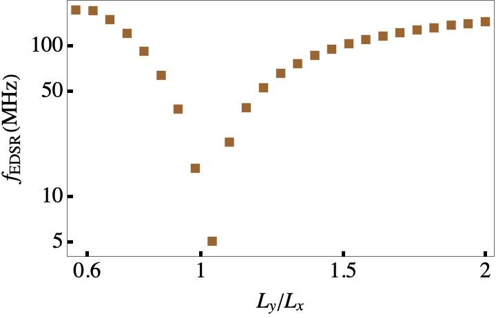
(a)

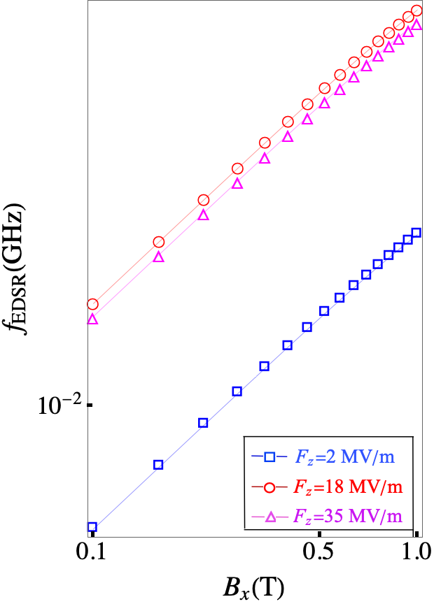
(b)

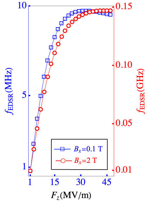
(c)

Figure 7: a)Variation of the EDSR Rabi frequency $f_{\text{EDSR}}$ with the aspect ratio $L_{y}/L_{x}$ of the hole QD. The confinement in x is fixed at $L_{x}{=}50\text{nm}$ while $L_{y}$ is varied. The calculation is done for $B_{x}{=}0.7\text{T}$. The EDSR driving field is applied along the $\hat{x}$-direction. $f_{\text{EDSR}}$ is a minimum when the dot is circular, i.e. $L_{x}{=}L_{y}{=}50\text{nm}$, while elliptical dots show an improvement of $>\!1$ order of magnitude in the EDSR spin-flip rate at high ellipticities. b) Linear monotonic dependence of $f_{\text{EDSR}}$ on the applied in-plane magnetic field $B_{x}$ for an elliptical dot with $L_{y}/L_{x}{=}2,\,L_{x}{=}50\text{nm}$ for three different values of the top gate potential: $F_{z}{=}2\,\text{MV/m}$, $F_{z}{=}18\,\text{MV/m}$ and $F_{z}{=}35\,\text{MV/m}$. c) Variation in $f_{\text{EDSR}}$ with the top gate electric field for an elliptical dot at low ($0.1\,\text{T}$) and high ($2\,\text{T}$) in-plane magnetic fields, displaying a maximum EDSR Rabi frequency at $F_{z}{=}18\,\text{MV/m}$ and $F_{z}{=}21\,\text{MV/m}$, respectively.

IV Elliptical Quantum dot

Introducing asymmetry into the planar confinement, i.e. having one lateral confinement potential stronger than the other will bring in additional sources of structure inversion asymmetry (SIA). For such elliptical hole QDs, the resultant Rashba spin-orbit interaction is stronger, bridging the gap between planar QD and nanowires Bosco et al. (2021b) in terms of fast gate operations. A theoretical understanding of QD ellipticity for holes is thus important. Insight into our numerical results can be obtained from the effective $2{\times}2$ spin-orbit Hamiltonian in Eqn. 8, which we rewrite as:

$$H_{SO} {=} \alpha_{R2}\!\left[k_{+}^{3}\sigma_{-}{-}k_{-}^{3}\sigma_{+}\right]\!+\!\alpha_{R3}\!\left[\{k_{+}^{2},k_{-}\}\sigma_{+}{-}\{k_{+},k_{-}^{2}\}\sigma_{-}\right]$$ (11)

$$\text{where,}\ \,\,\ \alpha_{R2}{=}\frac{e\hbar^{4}}{m_{0}^{2}}\gamma_{3}\overline{\gamma}S_{hh};\ \,\alpha_{R3}{=}\frac{e\hbar^{4}}{m_{0}^{2}}\gamma_{3}\delta S_{hh};$$

with the spherical Luttinger parameter $\overline{\gamma}{=}(\gamma_{2}+\gamma_{3})/2$, the cubic-symmetry parameter $\overline{\delta}{=}(\gamma_{3}-\gamma_{2})/2$, and $S_{hh}$ the sub-band interaction in $3^{\text{rd}}$ order perturbation theory (Appendix. B). In a circular dot the cubic-symmetry correction $\alpha_{R3}$ is responsible for EDSR, while the spherical term $\alpha_{R2}$ does not contribute. In contrast, in an elliptical dot the $\alpha_{R2}$ term is nonzero. From Eqn. 11, $\alpha_{R3}=(\delta/\overline{\gamma})\,\alpha_{R2}$; using the lattice parameters of Ge we evaluate $\alpha_{2}{\approx}10\,\alpha_{3}$. We present the results for a dot size of $L_{z}{=}11\,\text{nm}$, $L_{x}{=}50\,\text{nm}$, and varying $L_{y}$. Fig. 7a shows the variation of the EDSR Rabi frequency with the aspect ratio $L_{x}/L_{y}$, showing that an increase in the aspect ratio results in a larger Rabi frequency. The qubit Zeeman splitting is linear in the applied in-plane magnetic field, similar to the circular case. The relaxation rate varies as $B^{3}$. The EDSR Rabi frequency is linear in $B$ (Fig. 7b), which is reminiscent of out-of-plane $B$-field operation in presence of strong SIA; and the Rabi frequency exhibits a maximum as a function of $F_{z}$ (Fig. 7c).

V $\bm{g}$-factor anisotropy of elliptical QD and comparison with experiment

The in-plane $g$-factor of an elliptical dot is strongly anisotropic and exhibits an oscillatory behaviour as the magnetic field is rotated in the plane. We compare the predicted variation of the $g$-factor with experimentally measured values from EDSR in a planar germanium hole qubit. The qubit sample is a gate-defined double quantum dot in a Ge/Si_0.2Ge_0.8 heterostructure. (See Ref. 64 for further sample info). The dots are assumed to be elliptical, with a slight misalignment of their semi-major axes.

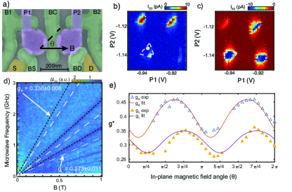
Figure 8: a) Sample scanning electron microscope (SEM) image of a gate-defined Ge double dot. b), c) Bias triangles (dashed) in forward and reverse bias respectively. Pauli spin blockade is visible in the transition marked by a yellow circle. d) g-factors measured via EDSR for the magnetic field direction indicated in part a) (black solid arrow). e) Comparison of the g-factor measured via EDSR with the theoretical prediction. The experimental results for $g$-factor anisotropy in Ref.115 are presented as scatter plots of effective $g$-factor ($g^{*}$) vs. the in-plane magnetic field angular orientation w.r.t. the double dot transport direction ($\theta$). We use triangular markers to denote the experimental data in scatter plots, while the solid fit lines are generated using the theoretical model in Sec. II. The $g$-factor for the left dot is denoted by $g_{L}$ (empty blue triangular experimental data points, solid red theoretical fit line), while the right dot $g$-factor is denoted by $g_{R}$ (filled yellow triangular experimental data points, solid purple theoretical fit line).

Fig. 8a shows a false colour SEM of the gate design. Plunger gates (purple) are used to define the two dots, while the barrier gates (green) are used to control coupling to the leads and between the dots. Metal ohmic contacts (yellow) act as a reservoir for holes. By negatively biasing the barrier and plunger gates, the sample can be tuned to the few hole regime. The relative angle between the applied magnetic field direction in the plane and the double dot transport direction is denoted by $\theta$. Bias triangles of the double dot measured via transport for positive and negative bias are shown in Fig. 8b and Fig. 8c. A region of Pauli spin blockade is visible at the base of one charge transition as indicated by a yellow circle. By applying an external magnetic field and a microwave tone to the P2 gate, we are able to drive spin rotations via EDSR when the microwave frequency matches the Larmor frequency ($\hbar f{=}g\mu_{B}B$). These spin rotations lift the Pauli spin blockade, causing a change in the current through the double dot. Using a lock-in amplifier, we measure the difference in current through the double dot when the microwave is on vs off. Fig. 8d shows the change in the leakage current for the double quantum dot with the external magnetic field applied in the direction indicated in Fig. 8a. Clear EDSR lines are visible for both dots, and both single and multi photon lines can be seen. From the slope of these resonance lines the g-factor can be calculated for each dot. Using this technique, we measure the g-factor as a function of field angle by rotating a magnetic field of $B{=}0.7\,\text{T}$ in the 2D plane. Fig. 8e shows the results of this measurement for both quantum dots, revealing an oscillatory variation in the g-factor as a function of in-plane magnetic field angle. The direction of $\theta$ is shown in Fig. 8a.

Using the model developed in Sec. II, we fit to the experimental data. For both dots we use the same size, shape and strain. We are able to account for the difference in g-factor between the dots by considering only a rotation of the dot axes in-plane and a change in the magnitude of the vertical electric field. A full list of fitting parameters is given in Table 1. The maximum value of the g-factor is not aligned with the external magnetic field or sample axes, and is also different for the left and right dots. To account for this, we introduce a phase shift angle ($\theta_{ps}$) which effectively rotates the axes of the quantum dots. Here $\theta_{ps,l}{=}\frac{3\pi}{4}$ and $\theta_{ps,r}{=}\frac{5\pi}{8}$ The magnitude of the g-factor is also different for each dot. This is accounted for by changing the vertical electric field applied to each dot. Here we use 10MV/m for the left dot and 45MV/m for the right dot. The results of the fits for both dots are shown by the solid lines in Fig 8 e).

Fitting Parameters	values
Left QD in-plane dimensions	$40\,\text{nm}{\times}30\,\text{nm}$
Right QD in-plane dimensions	$40\,\text{nm}{\times}30\,\text{nm}$
Left dot perpendicular confinement ($L_{z,l}$)	$10\,\text{nm}$
Right dot perpendicular confinement ($L_{z,r}$)	$10\,\text{nm}$
Left dot Top-gate voltage ($F_{z,l}$)	$10\,\text{MV/m}$
Right dot Top-gate voltage ($F_{z,r}$)	$45\,\text{MV/m}$
Left dot phase shift $\theta_{ps,l}$	$\frac{3\pi}{4}$
Right dot phase shift $\theta_{ps,r}$	$\frac{5\pi}{8}$
Left dot uni-axial compressive strain $\varepsilon_{xx,l}$	$-0.006$
Right dot uni-axial compressive strain $\varepsilon_{xx,r}$	$-0.006$
Applied magnetic field magnitude $B$	$0.7\,\text{T}$

Table 1: List of the parameters used to fit the analytical model to the experimental $g$-factor anisotropy data in Fig. 8e. While the choices of phase shift angles ($\theta_{ps}$) explain the experimental artifact of relative misalignment of the two dots; the top-gate voltages ($F_{z}$) are tuned to match the $g$-factor oscillation amplitudes of the dots. We stress however that the choice of fitting parameters given in this table for Fig. 8e is not unique. A possible set of parameters that yields a similar theoretical fitting of the experimental data in Fig. 8e are listed in appendix E.

The theoretical fit in Fig. 8e shows good agreement between the phase shift angle $\theta_{ps}$ parameter choices and B-field angular orientations where the experimental $g$-factors are maximum. In other words, the largest value of the $g$-factor occurs when the magnetic field is parallel to the semi-major axis of the elliptical hole QD. This behaviour is consistent with the effective in-plane $g$-factor being primarily the result of coupling to higher excited states brought about by the orbital magnetic field terms. We note that inhomogeneous strain in the sample, or the Ge/SiGe heterostructure interface induced roughness and disorder, or a misalignment of the sample with respect to the in-plane B-field (since $g_{\perp}\gg g_{\parallel}$) could potentially lead to significant modulation of the $g$-tensor. We can rule out the latter, since there is a different phase shift for the left and right dots in Fig. 8e. The effects of strain and inhomogeneities on $g$-factor anisotropy will be considered in a future publication.

VI Conclusions and Outlook

We have presented a generalised, semi-analytical model that fully describes the electrical operation of a planar germanium hole qubit in presence of an in-plane magnetic field. A comprehensive theory for spin manipulation via electron dipole spin resonance (EDSR) is given: surface inversion asymmetry (SIA) mediated fast EDSR is a result of the $\mathbf{k}\cdot\mathbf{p}$ coupling of the heavy hole ground state to higher energy light hole bands. The EDSR rate is linear in $B$ with important nonlinear corrections due to orbital mixing. Qubit relaxation is induced by acoustic phonons and the relaxation rate $1/T_{1}$ has terms with $B^{3},\,B^{4},\,B^{5}$ dependence, again reflecting the importance of the orbital mixing. In-plane operation demonstrates an excellent trade-off between relaxation and EDSR. The in-plane $g$-factor is strongly anisotropic and oscillates as the magnetic field is rotated in the plane. Random telegraph noise from charges in the plane of the quantum well results in decoherence, with an optimal top gate potential where it is insensitive to $\Delta F_{z}$; although the in-plane magnetic field exposes the qubit to $x-y$ electric field of the fluctuator. Hence, in contrast to the case of out-of-plane magnetic fields, coherence sweet spots cannot be identified in an in-plane $B$ for a qubit exposed to electric field fluctuations in all spatial directions. For an elliptical QD of aspect ratio $L_{y}/L_{x}{=}2$, EDSR is shown to be faster by an order of magnitude compared to a circular dot of $L_{x}{=}50\,\text{nm}$ radius; and the non-linear correction to EDSR is suppressed as rotational asymmetry induces more SIA Rashba.

Acknowledgments. This project is supported by the Australian Research Council Centre of Excellence in Future Low-Energy Electronics Technologies (project number CE170100039) and Discovery Project DP200100147. We acknowledge stimulating discussions with S. Das Sarma, M. Russ, X. Hu, and S. Liles.

Appendix A Gauge Invariance

The hole motion in the topmost valence band is described by the $4{\times}4$ Luttinger-Kohn (LK) Hamiltonian, which in the general operator form is given by:

$$H_{LK} = \frac{\hbar^{2}}{2m_{0}}\left[\left(\gamma_{1}+\frac{5\gamma_{2}}{2}\right)k^{2}-2\gamma_{2}(k_{x}^{2}J_{x}^{2}+k_{y}^{2}J_{y}^{2}+k_{z}^{2}J_{z}^{2})-4\gamma_{3}\left(\{k_{x},k_{y}\}\{J_{x},J_{y}\}+c.p.\right)\right]$$ (A12)

Expanding the anti-commutators, LK Hamiltonian has the form:

$$H_{LK} = \frac{\hbar^{2}}{2m_{0}}\left[\left(\gamma_{1}+\frac{5\gamma_{2}}{2}\right)(k_{x}^{2}+k_{y}^{2}+k_{z}^{2})-2\gamma_{2}(k_{x}^{2}J_{x}^{2}+k_{y}^{2}J_{y}^{2}+k_{z}^{2}J_{z}^{2})-4\gamma_{3}\left(\left(\frac{k_{x}k_{y}+k_{y}k_{x}}{2}\right)\left(\frac{J_{x}J_{y}+J_{y}J_{x}}{2}\right)\right.\right.$$ (A13)

$$+\left(\frac{k_{y}k_{z}+k_{z}k_{y}}{2}\right)\left(\frac{J_{y}J_{z}+J_{z}J_{y}}{2}\right)\left.\left.+\left(\frac{k_{x}k_{z}+k_{z}k_{x}}{2}\right)\left(\frac{J_{x}J_{z}+J_{z}J_{x}}{2}\right)\right)\right]$$

with $m_{0}$ notifying bare electron mass, $\gamma_{1}{=}13.38$, $\gamma_{2}{=}4.24$ and $\gamma_{3}{=}5.69$ are Luttinger parameters. We have tried two different gauges: $\frac{1}{2}\mathbf{B}\times\mathbf{r}$ and gauge choice from Loss et al.Kloeffel et al. (2018)

A.1 Gauge 1:

In presence of magnetic field, the momentum correction would be: $\mathbf{k}\rightarrow\left(\mathbf{k}+\frac{e\mathbf{A}}{\hbar}\right)$. We use the gauge (symmetric in z, Landau in x-y) $\mathbf{A}=-\frac{1}{2}B_{z}y\mathbf{\hat{e}_{x}}+\frac{1}{2}B_{z}x\mathbf{\hat{e}_{y}}+(B_{x}y-B_{y}x)\mathbf{\hat{e}_{z}}$.

Momentum Correction:

1. The components of corrected momentum:

   $$k_{x} \rightarrow \left(k_{x}-\frac{eB_{z}}{2\hbar}y\right)\,,\,k_{y}\rightarrow\left(k_{y}+\frac{eB_{z}}{2\hbar}x\right)\,,\,k_{z}\rightarrow\left(k_{z}+\frac{eB_{x}}{\hbar}y-\frac{eB_{y}}{\hbar}x\right)$$

   where, $\mathbf{k}=-\iota\mathbf{\partial}$. For $B_{y}=0,\,B_{z}=0$; $\text{we write: }\,k_{x}\rightarrow k_{x}\,,\,k_{y}\rightarrow k_{y}\,,\,k_{z}\rightarrow\left(k_{z}+\frac{eB_{x}}{\hbar}y\right)$

2. We evaluate $k_{i}^{2}$ terms below:

   $$k_{x}^{2} \Rightarrow k_{x}^{2}\,,\,k_{y}^{2}\Rightarrow k_{y}^{2}\,,\,k_{z}^{2}\Rightarrow\left(k_{z}^{2}+\frac{2eB_{x}yk_{z}}{\hbar}+\frac{e^{2}B_{x}^{2}y^{2}}{\hbar^{2}}\right)$$ (A14)

   and the cross-terms $k_{i}k_{j}$ are:

   $$k_{x}k_{y}\Rightarrow k_{x}k_{y};\,k_{y}k_{z}\Rightarrow\left(k_{y}k_{z}+\frac{eB_{x}}{\hbar}\{y,k_{y}\}\right);\,k_{x}k_{z}\Rightarrow\left(k_{x}k_{z}+\frac{eB_{x}yk_{x}}{\hbar}\right)$$ (A15)

3. Using these corrections, the LK Hamiltonian is:

   $$H_{LK}=\bigg{[}\,\overline{\gamma_{1}+\frac{5\gamma_{2}}{2}}\left(k_{x}^{2}+k_{y}^{2}+k_{z}^{2}+\frac{2eB_{x}yk_{z}}{\hbar}+\frac{e^{2}B_{x}^{2}y^{2}}{\hbar^{2}}\right)-2\gamma_{2}\left(k_{x}^{2}J_{x}^{2}+k_{y}^{2}J_{y}^{2}+\left(k_{z}^{2}+\frac{2eB_{x}yk_{z}}{\hbar}+\frac{e^{2}B_{x}^{2}y^{2}}{\hbar^{2}}\right)J_{z}^{2}\right)$$

   $$-4\gamma_{3}\left(k_{x}k_{y}\{J_{x},J_{y}\}+\left(k_{y}k_{z}+\frac{eB_{x}}{\hbar}\{y,k_{y}\}\right)\{J_{y},J_{z}\}+\left(k_{x}k_{z}+\frac{eB_{x}yk_{x}}{\hbar}\right)\{J_{z},J_{x}\}\right)\bigg{]}\frac{\hbar^{2}}{2m_{0}}$$ (A16)

   where,

   $$H_{LK}^{11/22} = \frac{\hbar^{2}}{2m_{0}}\bigg{[}(\gamma_{1}-2\gamma_{2})\left(k_{z}^{2}+\frac{2eB_{x}yk_{z}}{\hbar}+\frac{e^{2}B_{x}^{2}y^{2}}{\hbar^{2}}\right)+(\gamma_{1}+\gamma_{2})(k_{x}^{2}+k_{y}^{2})\bigg{]}$$

   $$H_{LK}^{33/44} = \frac{\hbar^{2}}{2m_{0}}\bigg{[}(\gamma_{1}+2\gamma_{2})\left(k_{z}^{2}+\frac{2eB_{x}yk_{z}}{\hbar}+\frac{e^{2}B_{x}^{2}y^{2}}{\hbar^{2}}\right)+(\gamma_{1}-\gamma_{2})(k_{x}^{2}+k_{y}^{2})\bigg{]}$$

   $$H_{LK}^{13}=L = -\sqrt{3}\frac{\hbar^{2}\gamma_{3}}{m_{0}}\bigg{[}\left(k_{x}k_{z}+\frac{eB_{x}yk_{x}}{\hbar}\right)-i\left(k_{y}k_{z}+\frac{eB_{x}}{\hbar}\{y,k_{y}\}\right)\bigg{]}$$

   $$H_{LK}^{14}=M = \frac{\sqrt{3}\hbar^{2}}{2m_{0}}\left[-\gamma_{2}\left(k_{x}^{2}-k_{y}^{2}\right)+2i\gamma_{3}k_{x}k_{y}\right]$$

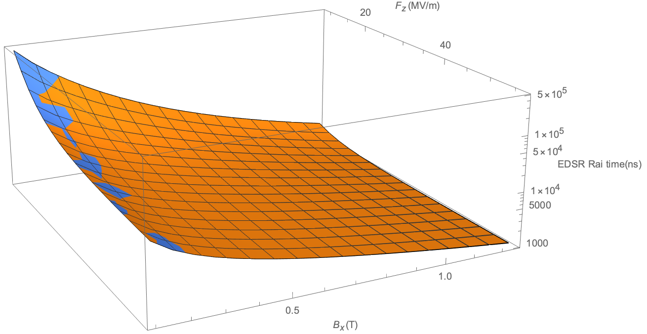
Figure A1: EDSR time $T_{\pi}$ (ns) vs. top gate field $F_{z}$ and in-plane magnetic field $B_{x}$.

A.2 Gauge 2:

In this section, we use the symmetric gauge ($\frac{1}{2}\mathbf{B}\times\mathbf{r}$): $\mathbf{A}=\frac{1}{2}(B_{y}z-B_{z}y)\mathbf{\hat{e}_{x}}+\frac{1}{2}(B_{z}x-B_{x}z)\mathbf{\hat{e}_{y}}+\frac{1}{2}(B_{x}y-B_{y}x)\mathbf{\hat{e}_{z}}$.

Momentum Correction:

1. The components of corrected momentum with $B_{y}=0\,,B_{z}=0$:

   $$k_{x}\rightarrow k_{x},\,k_{y}\rightarrow\left(k_{y}-\frac{eB_{x}}{2\hbar}z\right)\,,\,k_{z}\rightarrow\left(k_{z}+\frac{eB_{x}}{2\hbar}y\right)\,\text{where,}\,\mathbf{k}=-\iota\partial.$$ (A18)

2. We evaluate $k_{i}^{2}$ terms below:

   $$k_{x}^{2} \Rightarrow k_{x}^{2}\,,\,k_{y}^{2}\Rightarrow\left(k_{y}^{2}-\frac{eB_{x}zk_{y}}{\hbar}+\frac{e^{2}B_{x}^{2}z^{2}}{4\hbar^{2}}\right)\,,\,k_{z}^{2}\Rightarrow\left(k_{z}^{2}+\frac{eB_{x}yk_{z}}{\hbar}+\frac{e^{2}B_{x}^{2}y^{2}}{4\hbar^{2}}\right)$$ (A19)

   and the cross-terms $k_{i}k_{j}$ are:

   $$k_{x}k_{y} \Rightarrow \!\left(\!k_{x}k_{y}-\frac{eB_{x}zk_{x}}{2\hbar}\!\right);\!k_{y}k_{z}\Rightarrow\!\left(\!k_{y}k_{z}+\frac{eB_{x}}{2\hbar}(\{y,k_{y}\}-\{z,k_{z}\})-\frac{e^{2}B_{x}^{2}}{4\hbar^{2}}yz\right)\!;\!k_{x}k_{z}\Rightarrow\left(\!k_{x}k_{z}+\frac{eB_{x}yk_{x}}{2\hbar}\right)$$ (A20)

3. Using these corrections, the LK Hamiltonian terms become:

   $$H_{LK}=\frac{\hbar^{2}}{2m_{0}}\bigg{[}\left(\gamma_{1}+\frac{5\gamma_{2}}{2}\right)\left(k_{x}^{2}+k_{y}^{2}-\frac{eB_{x}zk_{y}}{\hbar}+\frac{e^{2}B_{x}^{2}z^{2}}{4\hbar^{2}}+k_{z}^{2}+\frac{eB_{x}yk_{z}}{\hbar}+\frac{e^{2}B_{x}^{2}y^{2}}{4\hbar^{2}}\right)$$

   $$-2\gamma_{2}\left(k_{x}^{2}J_{x}^{2}+\left(k_{y}^{2}-\frac{eB_{x}zk_{y}}{\hbar}+\frac{e^{2}B_{x}^{2}z^{2}}{4\hbar^{2}}\right)J_{y}^{2}+\left(k_{z}^{2}+\frac{eB_{x}yk_{z}}{\hbar}+\frac{e^{2}B_{x}^{2}y^{2}}{4\hbar^{2}}\right)J_{z}^{2}\right)-4\gamma_{3}\left(\left(k_{x}k_{y}-\frac{eB_{x}zk_{x}}{2\hbar}\right)\{J_{x},J_{y}\}\right.$$

   $$\left.+\left(k_{y}k_{z}+\frac{eB_{x}}{2\hbar}\{y,k_{y}\}-\frac{eB_{x}}{2\hbar}\{z,k_{z}\}-\frac{e^{2}B_{x}^{2}}{4\hbar^{2}}yz\right)\{J_{y},J_{z}\}+\left(k_{x}k_{z}+\frac{eB_{x}yk_{x}}{2\hbar}\right)\{J_{z},J_{x}\}\right)\bigg{]}$$ (A21)

   where,

   $$H_{LK}^{11/22}=\frac{\hbar^{2}}{2m_{0}}\left[(\gamma_{1}-2\gamma_{2})\left(k_{z}^{2}+\frac{2eB_{x}yk_{z}}{\hbar}+\frac{e^{2}B_{x}^{2}y^{2}}{\hbar^{2}}\right)+(\gamma_{1}+\gamma_{2})\left(k_{x}^{2}+k_{y}^{2}-\frac{eB_{x}zk_{y}}{\hbar}+\frac{e^{2}B_{x}^{2}z^{2}}{4\hbar^{2}}\right)\right]$$ (A22)

   $$H_{LK}^{33/44}=\frac{\hbar^{2}}{2m_{0}}\left[(\gamma_{1}+2\gamma_{2})\left(k_{z}^{2}+\frac{2eB_{x}yk_{z}}{\hbar}+\frac{e^{2}B_{x}^{2}y^{2}}{\hbar^{2}}\right)+(\gamma_{1}-\gamma_{2})\left(k_{x}^{2}+k_{y}^{2}-\frac{eB_{x}zk_{y}}{\hbar}+\frac{e^{2}B_{x}^{2}z^{2}}{4\hbar^{2}}\right)\right]$$ (A23)

   $$H_{LK}^{13}=L=-\sqrt{3}\frac{\hbar^{2}\gamma_{3}}{m_{0}}\bigg{[}\left(k_{x}k_{z}+\frac{eB_{x}yk_{x}}{2\hbar}\right)-i\left(k_{y}k_{z}+\frac{eB_{x}}{2\hbar}\{y,k_{y}\}-\frac{eB_{x}}{2\hbar}\{z,k_{z}\}-\frac{e^{2}B_{x}^{2}}{4\hbar^{2}}yz\right)\bigg{]}$$

   $$H_{LK}^{14}=M=\frac{\sqrt{3}\hbar^{2}}{2m_{0}}\bigg{[}-\gamma_{2}\left(k_{x}^{2}-k_{y}^{2}+\frac{eB_{x}zk_{y}}{\hbar}-\frac{e^{2}B_{x}^{2}z^{2}}{4\hbar^{2}}\right)+2i\gamma_{3}\left(k_{x}k_{y}-\frac{eB_{x}zk_{x}}{2\hbar}\right)\bigg{]}$$ (A24)

Appendix B Schreiffer-Wolff Transformation

In the effective $2\times 2$ system Hamiltonian given by Eqn. 8, $H_{0}+V(x,y)$ produces the quantized in-plane energies. We consider a basis with following in-plane states:

$$\left\{\frac{e^{-\left(\!\frac{x^{2}}{2L_{x}^{2}}{+}\frac{y^{2}}{2L_{y}^{2}}\right)}}{\sqrt{\pi L_{x}L_{y}}},\,\frac{\sqrt{2}y\,e^{-\left(\!\frac{x^{2}}{2L_{x}^{2}}{+}\frac{y^{2}}{2L_{y}^{2}}\right)}}{\sqrt{\pi L_{y}^{3}L_{x}}},\,\frac{\sqrt{2}x\,e^{-\left(\!\frac{x^{2}}{2L_{x}^{2}}{+}\frac{y^{2}}{2L_{y}^{2}}\right)}}{\sqrt{\pi L_{x}^{3}L_{y}}}\right\}\otimes\left\{\uparrow,\,\downarrow\right\}$$ (B25)

where the spatial states are the first three harmonic oscillator product states: $(n,m){=}\{(0,0),(0,1),(1,0)\}$, we denote the orbital energies of these states as $E_{0},\,E_{1},\,E_{1}$. The spinors are the effective spin-up and spin-down states of the 2D hole qubit, and gives $\pm g_{\parallel}\mu_{B}B_{x}$ Zeeman energies for the up and down spin states. The spin-orbit interactions can be listed as:

$$H_{SO}{=}i\alpha_{R1}(k_{-}\sigma_{-}{-}k_{+}\sigma_{+})\!+i\alpha_{R2}\left(k_{+}^{3}\sigma_{-}-k_{-}^{3}\sigma_{+}\right)\!+i\alpha_{R3}\left(\{k_{+},k_{-}^{2}\}\sigma_{-}\!-\!\{k_{+}^{2},k_{-}\}\sigma_{+}\right)\!+i\alpha_{R4}\left(\{k_{z}^{2},k_{-}\}\sigma_{-}{-}\{k_{z}^{2},k_{+}\}\sigma_{+}\right)$$ (B26)

The $k$-linear Rashba terms come from the coupling of the bonding VB $p$-orbitals to the antibonding CB $p$-orbitals, which is very small. In the Luttinger formalism thus the $\alpha_{R1},\,\alpha_{R4}$ terms vanish. The nonzero contributions are:

$$H_{SO}{=}i\alpha_{R2}\left(k_{+}^{3}\sigma_{-}-k_{-}^{3}\sigma_{+}\right)\!+i\alpha_{R3}\left(\{k_{+},k_{-}^{2}\}\sigma_{-}\!-\!\{k_{+}^{2},k_{-}\}\sigma_{+}\right)$$ (B27)

the spin-orbit matrix elements are calculated below:

$$\left\langle(0,0)\uparrow\right|H_{SO}\left|(0,1)\downarrow\right\rangle {=} -i\alpha_{R2}\left\langle(0,0)\uparrow\right|k_{-}^{3}\sigma_{+}\left|(0,1)\downarrow\right\rangle+i\alpha_{R3}\left\langle(0,0)\uparrow\right|k_{+}k_{-}k_{+}\sigma_{+}\left|(0,1)\downarrow\right\rangle$$ (B28)

$${=} -i\alpha_{R2}\left\langle(0,0)\right|k_{-}^{3}\left|(0,1)\right\rangle+i\alpha_{R3}\left\langle(0,0)\right|k_{+}k_{-}k_{+}\left|(0,1)\right\rangle$$

$${=} \frac{-3i\alpha_{R2}}{2\sqrt{2}L_{y}^{3}}\left(1-\frac{L_{y}^{2}}{L_{x}^{2}}\right)+\frac{i\alpha_{R3}}{2\sqrt{2}L_{y}^{3}}\left(1+3\frac{L_{y}^{2}}{L_{x}^{2}}\right)=R_{c}$$

$$\left\langle(0,0)\uparrow\right|H_{SO}\left|(1,0)\downarrow\right\rangle {=} -i\alpha_{R2}\left\langle(0,0)\uparrow\right|k_{-}^{3}\sigma_{+}\left|(1,0)\downarrow\right\rangle+i\alpha_{R3}\left\langle(0,0)\uparrow\right|k_{+}k_{-}k_{+}\sigma_{+}\left|(1,0)\downarrow\right\rangle$$ (B29)

$${=} -i\alpha_{R2}\left\langle(0,0)\right|k_{-}^{3}\left|(0,1)\right\rangle+i\alpha_{R3}\left\langle(0,0)\right|k_{+}k_{-}k_{+}\left|(0,1)\right\rangle$$

$${=} \frac{-3\alpha_{R2}}{2\sqrt{2}L_{x}L_{y}^{2}}\left(1-\frac{L_{y}^{2}}{L_{x}^{2}}\right)+\frac{\alpha_{R3}}{2\sqrt{2}L_{x}L_{y}^{2}}\left(1+3\frac{L_{y}^{2}}{L_{x}^{2}}\right)=R_{r}$$

The ac electric field $eE_{x}(t)x$ is spin-conserving and connects the states $(0,0)$ and $(1,0)$. Putting all of it together, the $6\times 6$ Hamiltonian would be:

$$H^{\prime}=\begin{pmatrix}E_{0}-\frac{1}{2}g_{\parallel}\mu_{B}B_{x}&0&0&R_{c}&eE_{x}a&R_{r}\\ 0&E_{0}+\frac{1}{2}g_{\parallel}\mu_{B}B_{x}&R_{c}^{*}&0&-R_{r}&eE_{x}a\\ 0&R_{c}&E_{1}-\frac{1}{2}g_{\parallel}\mu_{B}B_{x}&0&0&0\\ R_{c}^{*}&0&0&E_{1}+\frac{1}{2}g_{\parallel}\mu_{B}B_{x}&0&0\\ eE_{x}a&-R_{r}&0&0&E_{1}-\frac{1}{2}g_{\parallel}\mu_{B}B_{x}&0\\ R_{r}&eE_{x}a&0&0&0&E_{1}+\frac{1}{2}g_{\parallel}\mu_{B}B_{x}\end{pmatrix}$$ (B30)

$2^{\text{nd}}$ order perturbation theory gives the EDSR matrix element as:

$$\tilde{H}_{12} = \sum_{j=3}^{6}\frac{1}{2}H^{\prime}_{1j}H^{\prime}_{j2}\left(\frac{1}{\epsilon_{1}-\epsilon_{j}}+\frac{1}{\epsilon_{2}-\epsilon_{j}}\right)=\frac{1}{2}H^{\prime}_{15}H^{\prime}_{52}\left(\frac{1}{\epsilon_{1}-\epsilon_{5}}+\frac{1}{\epsilon_{2}-\epsilon_{5}}\right)+\frac{1}{2}H^{\prime}_{16}H^{\prime}_{62}\left(\frac{1}{\epsilon_{1}-\epsilon_{6}}+\frac{1}{\epsilon_{2}-\epsilon_{6}}\right)$$ (B31)

$$= -\frac{1}{2}eE_{x}a\,R_{r}\left(\frac{1}{-\Delta_{01}}+\frac{1}{-\Delta_{01}+Z}\right)+\frac{1}{2}eE_{x}a\,R_{r}\left(\frac{1}{-\Delta_{01}-Z}+\frac{1}{-\Delta_{01}}\right)$$

$$= eE_{x}a\,R_{r}\left(\frac{1}{\Delta_{01}\left(1-\frac{Z}{\Delta_{01}}\right)}-\frac{1}{\Delta_{01}\left(1+\frac{Z}{\Delta_{01}}\right)}\right)=(eE_{x}a\,R_{r}Z)/\Delta_{01}^{2}$$

Where we have used $Z=g_{\parallel}\mu_{B}B_{x}$, $\Delta_{01}=E_{1}-E_{0}$. This gives $\tilde{H}_{12}{\propto}B_{x}$, explaining the linear magnetic field dependence of EDSR.

From Eqn. B28, B29, the $\alpha_{2}$ term vanishes when $L_{x}=L_{y}$ i.e. for a symmetric dot, while it is strongly nonzero for an elliptical dot; making the linear $B_{x}$-dependence stronger.

Appendix C Bulk Phonon mediated Relaxation Rate Analytics

The total strain in the $4\times 4$ Luttinger-Kohn-Bir-Pikus formalism is given as:

$$H^{LKBP}_{strain}(\bm{r})=\begin{pmatrix}P_{\varepsilon}(\bm{r})+Q_{\varepsilon}(\bm{r})&0&L_{\varepsilon}(\bm{r})&M_{\varepsilon}(\bm{r})\\ 0&P_{\varepsilon}(\bm{r})+Q_{\varepsilon}(\bm{r})&M_{\varepsilon}(\bm{r})^{*}&-L_{\varepsilon}(\bm{r})^{*}\\ L_{\varepsilon}(\bm{r})^{*}&M_{\varepsilon}(\bm{r})&P_{\varepsilon}(\bm{r})-Q_{\varepsilon}(\bm{r})&0\\ M_{\varepsilon}(\bm{r})^{*}&-L_{\varepsilon}(\bm{r})&0&P_{\varepsilon}(\bm{r})-Q_{\varepsilon}(\bm{r})\\ \end{pmatrix}$$ (C32)

where, $P_{\varepsilon}(\bm{r}){=}-a(\varepsilon_{xx}(\bm{r})+\varepsilon_{yy}(\bm{r})+\varepsilon_{zz}(\bm{r}))$, $Q_{\varepsilon}(\bm{r}){=}-\frac{b}{2}(\varepsilon_{xx}(\bm{r})+\varepsilon_{yy}(\bm{r})-2\varepsilon_{zz}(\bm{r}))$, $L_{\varepsilon}(\bm{r}){=}d(\varepsilon_{xz}(\bm{r})-i\varepsilon_{yz}(\bm{r}))$, $M_{\varepsilon}(\bm{r}){=}\left(\frac{\sqrt{3}}{2}b(\varepsilon_{xx}(\bm{r})-\varepsilon_{yy}(\bm{r}))-id\varepsilon_{xy}(\bm{r})\right)$. The non-zero static component of the strain tensor is given by $\varepsilon_{xx}=\varepsilon_{yy}=-0.006$, and $\varepsilon_{zz}=-\frac{C_{12}}{C_{11}}\varepsilon_{xx}$ with $C_{12}{=}44$ GPa, $C_{11}{=}126$ GPa. Considering the lattice deformation potential $\mathcal{D}(\bm{r})$, the ’local’ strain is given by:

$$\varepsilon_{i,j}^{\alpha}(\bm{r})=\frac{1}{2}\left(\frac{\partial u_{i}(\bm{r})}{\partial r_{j}}+\frac{\partial u_{j}(\bm{r})}{\partial r_{i}}\right),\ \ i,j\in\{x,y,z\}$$ (C33)

Here $\bm{u}$ vector designates the deformation field at the position $\bm{r}$. For a phonon traveling with wave vector $\mathbf{q}$ in the polarized state $\alpha$, the strain tensor is given by,

$$\varepsilon_{i,j}^{\alpha}(\bm{r})=\frac{i}{2}\sqrt{\frac{\hbar}{2V_{c}\rho\omega_{\mathbf{q},\alpha}}}q(\hat{c}_{i}^{\alpha}\hat{q}_{j}+\hat{c}_{j}^{\alpha}\hat{q}_{i})(e^{-i\mathbf{q}\cdot\mathbf{r}}a_{\mathbf{q},\alpha}+e^{i\mathbf{q}\cdot\mathbf{r}}a^{\dagger}_{\mathbf{q},\alpha})$$ (C34)

where $\hat{c}$ is the polarisation unit vector. We consider three polarisations with con-ordinate systems understood as $l\!:\!(r,\theta,\phi);\,t\!:\!\left(r,\theta+\frac{\pi}{2},\phi\right);\,w\!:\!\left(r,\frac{\pi}{2},\phi+\frac{\pi}{2}\right)$. Using $\omega_{\mathbf{q},\alpha}{=}\,v_{\alpha}q$,

$$\varepsilon_{i,j}^{\alpha}(\bm{r})=i\sqrt{\frac{\hbar}{2V_{c}\rho v_{\alpha}}}\sqrt{q}\mathcal{A}_{\varepsilon,ij}^{\alpha}e^{i\mathbf{q}\cdot\mathbf{r}}(a_{-\mathbf{q},\alpha}+a^{\dagger}_{\mathbf{q},\alpha})$$ (C35)

where $v_{\alpha}$ are the acoustic phonon velocities, and we assumed $\frac{1}{2}(\hat{c}_{i}^{\alpha}\hat{q}_{j}+\hat{c}_{j}^{\alpha}\hat{q}_{i})=\mathcal{A}_{\varepsilon,ij}^{\alpha}$. The matrix elements of $\mathcal{A}_{\varepsilon,ij}^{\alpha}$ are sketched out below:

$$\mathcal{A}_{\varepsilon}^{\alpha}=\frac{1}{2}\begin{pmatrix}2\hat{c}_{x}^{\alpha}\hat{q}_{x}&\hat{c}_{x}^{\alpha}\hat{q}_{y}+\hat{c}_{y}^{\alpha}\hat{q}_{x}&\hat{c}_{x}^{\alpha}\hat{q}_{z}+\hat{c}_{z}^{\alpha}\hat{q}_{x}\\ \hat{c}_{y}^{\alpha}\hat{q}_{x}+\hat{c}_{x}^{\alpha}\hat{q}_{y}&2\hat{c}_{y}^{\alpha}\hat{q}_{y}&\hat{c}_{y}^{\alpha}\hat{q}_{z}+\hat{c}_{z}^{\alpha}\hat{q}_{y}\\ \hat{c}_{z}^{\alpha}\hat{q}_{x}+\hat{c}_{x}^{\alpha}\hat{q}_{z}&\hat{c}_{z}^{\alpha}\hat{q}_{y}+\hat{c}_{y}^{\alpha}\hat{q}_{z}&2\hat{c}_{z}^{\alpha}\hat{q}_{z}\end{pmatrix}$$ (C36)

The phonon wave vector has the components $\overrightarrow{q}\rightarrow\{q\sin\theta\cos\phi,q\sin\theta\,\sin\phi,q\cos\theta\}$; so the unit vectors for $\bm{q}$ are given by: $\bm{\hat{}}{q}\rightarrow\{\sin\theta\cos\phi,\,\sin\theta\,\sin\phi,\,\cos\theta\}$. The polarization wave vectors are as follows:

• $\hat{c}^{l}\rightarrow q^{-1}\{q_{x},q_{y},q_{z}\}=\{\sin\theta\cos\phi,\,\sin\theta\cos\phi,\,\cos\theta\}$

• $\hat{c}^{t}\rightarrow q^{-1}(q_{x}^{2}+q_{y}^{2})^{-\frac{1}{2}}\{q_{x}q_{z},q_{y}q_{z},-(q_{x}^{2}+q_{y}^{2})\}=\{\cos\theta\cos\phi,\,\cos\theta\sin\phi,-\sin\theta\}$

• $\hat{c}^{w}\rightarrow(q_{x}^{2}+q_{y}^{2})^{-\frac{1}{2}}\{q_{y},-q_{x},0\}=\{-\sin\phi,\,\cos\phi,\,0\}$

We can write the matrix elements of $\mathcal{A}_{\varepsilon,ij}^{\alpha}$ for the three polarisations using the decompositions above:

$$\mathcal{A}_{\varepsilon}^{l} = \frac{1}{2}\begin{pmatrix}2\frac{q_{x}^{2}}{q^{2}}&2\frac{q_{x}q_{y}}{q^{2}}&2\frac{q_{x}q_{z}}{q^{2}}\\ 2\frac{q_{y}q_{x}}{q^{2}}&2\frac{q_{y}^{2}}{q^{2}}&2\frac{2q_{y}q_{z}}{q^{2}}\\ 2\frac{q_{z}q_{x}}{q^{2}}&2\frac{q_{z}q_{y}}{q^{2}}&2\frac{q_{z}^{2}}{q^{2}}\end{pmatrix}=\frac{1}{q^{2}}\begin{pmatrix}q_{x}^{2}&q_{x}q_{y}&q_{x}q_{z}\\ q_{y}q_{x}&q_{y}^{2}&q_{y}q_{z}\\ q_{z}q_{x}&q_{z}q_{y}&q_{z}^{2}\\ \end{pmatrix}$$

$$\mathcal{A}_{\varepsilon}^{t} = \frac{1}{2}\begin{pmatrix}2\frac{q_{z}}{q}\frac{q_{x}}{\sqrt{q_{x}^{2}+q_{y}^{2}}}\frac{q_{x}}{q}&2\frac{q_{z}}{q}\frac{q_{x}}{\sqrt{q_{x}^{2}+q_{y}^{2}}}\frac{q_{y}}{q}&\frac{q_{x}q_{z}}{q\sqrt{q_{x}^{2}+q_{y}^{2}}}\frac{q_{z}}{q}-\frac{\sqrt{q_{x}^{2}+q_{y}^{2}}}{q}\frac{q_{x}}{q}\\ 2\frac{q_{z}}{q}\frac{q_{x}}{\sqrt{q_{x}^{2}+q_{y}^{2}}}\frac{q_{y}}{q}&2\frac{q_{z}}{q}\frac{q_{y}}{\sqrt{q_{x}^{2}+q_{y}^{2}}}\frac{q_{y}}{q}&\frac{q_{y}q_{z}}{q\sqrt{q_{x}^{2}+q_{y}^{2}}}\frac{q_{z}}{q}-\frac{\sqrt{q_{x}^{2}+q_{y}^{2}}}{q}\frac{q_{y}}{q}\\ \frac{q_{x}q_{z}}{q\sqrt{q_{x}^{2}+q_{y}^{2}}}\frac{q_{z}}{q}-\frac{\sqrt{q_{x}^{2}+q_{y}^{2}}}{q}\frac{q_{x}}{q}&\frac{q_{z}^{2}q_{y}-q_{x}^{2}q_{y}-q_{y}^{3}}{q^{2}\sqrt{q_{x}^{2}+q_{y}^{2}}}&-2\frac{q_{z}}{q}\frac{\sqrt{q_{x}^{2}+q_{y}^{2}}}{q}\end{pmatrix}$$

$$\mathcal{A}_{\varepsilon}^{w} = \frac{1}{2}\begin{pmatrix}-2\frac{q_{y}}{\sqrt{q_{x}^{2}+q_{y}^{2}}}\frac{q_{x}}{q}&-\frac{q_{y}}{\sqrt{q_{x}^{2}+q_{y}^{2}}}\frac{q_{y}}{q}+\frac{q_{x}}{\sqrt{q_{x}^{2}+q_{y}^{2}}}\frac{q_{x}}{q}&-\frac{q_{y}}{\sqrt{q_{x}^{2}+q_{y}^{2}}}\frac{q_{z}}{q}\\ \frac{q_{x}^{2}-q_{y}^{2}}{q\sqrt{q_{x}^{2}+q_{y}^{2}}}&2\frac{q_{x}q_{y}}{q\sqrt{q_{x}^{2}+q_{y}^{2}}}&\frac{q_{x}q_{z}}{q\sqrt{q_{x}^{2}+q_{y}^{2}}}\\ -\frac{q_{y}q_{z}}{q\sqrt{q_{x}^{2}+q_{y}^{2}}}&\frac{q_{x}q_{z}}{q\sqrt{q_{x}^{2}+q_{y}^{2}}}&0\end{pmatrix}$$ (C37)

We wish to evaluate the angular integrals, so we write the matrices in terms of $\theta$ and $\phi$:

$$\mathcal{A}_{\varepsilon}^{l}=\begin{pmatrix}\sin^{2}\theta\cos^{2}\phi&\sin^{2}\theta\sin\phi\cos\phi&\sin\theta\cos\theta\cos\phi\\ \sin^{2}\theta\sin\phi\cos\phi&\sin^{2}\theta\sin^{2}\phi&\sin\theta\cos\theta\sin\phi\\ \sin\theta\cos\theta\cos\phi&\sin\theta\cos\theta\sin\phi&\cos^{2}\theta\end{pmatrix}$$

$$\mathcal{A}_{\varepsilon}^{t} = \frac{1}{2}\begin{pmatrix}2\cos\theta\cos\phi\sin\theta\cos\phi&2\cos\theta\cos\phi\sin\theta\sin\phi&\cos\theta\cos\phi\cos\theta-\sin^{2}\theta\cos\phi\\ 2\cos\theta\cos\phi\sin\theta\sin\phi&2\cos\theta\sin\phi\sin\theta\sin\phi&\cos\theta\sin\phi\cos\theta-\sin^{2}\theta\sin\phi\\ \cos\theta\cos\phi\cos\theta-\sin^{2}\theta\cos\phi&\cos\theta\sin\phi\cos\theta-\sin^{2}\theta\sin\phi&-2\sin\theta\cos\theta\end{pmatrix}$$

$$= \begin{pmatrix}\frac{1}{2}\sin 2\theta\cos^{2}\phi&\frac{1}{4}\sin 2\theta\sin 2\phi&\frac{1}{2}\cos 2\theta\cos\phi\\ \frac{1}{4}\sin 2\theta\sin 2\phi&\frac{1}{2}\sin 2\theta\sin^{2}\phi&\frac{1}{2}\cos 2\theta\sin\phi\\ \frac{1}{2}\cos 2\theta\cos\phi&\frac{1}{2}\cos 2\theta\sin\phi&-\frac{1}{2}\sin 2\theta\end{pmatrix}$$

$$\mathcal{A}_{\varepsilon}^{w} = \frac{1}{2}\begin{pmatrix}-2\sin\phi\sin\theta\cos\phi&-\sin\phi\sin\theta\sin\phi+\cos\phi\sin\theta\cos\phi&-\sin\phi\cos\theta\\ -\sin\phi\sin\theta\sin\phi+\cos\phi\sin\theta\cos\phi&2\cos\phi\sin\theta\sin\phi&\cos\phi\cos\theta\\ -\sin\phi\cos\theta&\cos\phi\cos\theta&0\end{pmatrix}$$ (C38)

$$= \frac{1}{2}\begin{pmatrix}-\sin 2\phi\sin\theta&\cos 2\phi\sin\theta&-\sin\phi\cos\theta\\ \cos 2\phi\sin\theta&\sin 2\phi\sin\theta&\cos\phi\cos\theta\\ -\sin\phi\cos\theta&\cos\phi\cos\theta&0\end{pmatrix}$$

The total hole-phonon Hamiltonian can be added as per the following equation:

$$H_{h-ph}^{\alpha}=\mathcal{D}_{11}^{\alpha}\mathcal{A}_{\varepsilon,11}^{\alpha}+\mathcal{D}_{12}^{\alpha}\mathcal{A}_{\varepsilon,12}^{\alpha}+\mathcal{D}_{13}^{\alpha}\mathcal{A}_{\varepsilon,13}^{\alpha}+\mathcal{D}_{22}^{\alpha}\mathcal{A}_{\varepsilon,22}^{\alpha}+\mathcal{D}_{23}^{\alpha}\mathcal{A}_{\varepsilon,23}^{\alpha}+\mathcal{D}_{33}^{\alpha}\mathcal{A}_{\varepsilon,33}^{\alpha}$$ (C39)

where $\alpha$ is the polarisation index, and $\mathcal{D}$ are the $4\times 4$ LK deformation potential matrices.

l-polarisation:

Putting in the local strain terms, we can write:

$$H_{h-ph}^{l}=i\sqrt{q}\sqrt{\frac{\hbar}{2V_{c}\rho v_{l}}}\begin{pmatrix}P_{\varepsilon}^{l}+Q_{\varepsilon}^{l}&0&L_{\varepsilon}^{l}&M_{\varepsilon}^{l}\\ 0&P_{\varepsilon}^{l}+Q_{\varepsilon}^{l}&M_{\varepsilon}^{l^{*}}&-L_{\varepsilon}^{l^{*}}\\ L_{\varepsilon}^{l^{*}}&M_{\varepsilon}^{l}&P_{\varepsilon}^{l}-Q_{\varepsilon}^{l}&0\\ M_{\varepsilon}^{l^{*}}&-L_{\varepsilon}^{l}&0&P_{\varepsilon}^{l}-Q_{\varepsilon}^{l}\end{pmatrix}e^{i\mathbf{q}\cdot\mathbf{r}}(a_{-\mathbf{q},l}+a^{\dagger}_{\mathbf{q},l})$$

where,

$$P_{\varepsilon}^{l} = -a(\sin^{2}\theta\cos^{2}\phi+\sin^{2}\theta\sin^{2}\phi+\cos^{2}\theta)=-a$$

$$Q_{\varepsilon}^{l} = -\frac{b}{2}(\sin^{2}\theta\cos^{2}\phi+\sin^{2}\theta\sin^{2}\phi-2\cos^{2}\theta)=-\frac{b}{2}(1-3\cos^{2}\theta)$$

$$L_{\varepsilon}^{l} = d(\sin\theta\cos\theta\cos\phi-i\sin\theta\cos\theta\sin\phi)=\frac{d}{2}\sin 2\theta\,e^{-i\phi}$$

$$M_{\varepsilon}^{l} = \frac{\sqrt{3}b}{2}(\sin^{2}\theta\cos^{2}\phi-\sin^{2}\theta\sin^{2}\phi)-id\sin\phi\cos\phi\sin^{2}\theta=\frac{\sqrt{3}b}{2}\sin^{2}\theta\cos 2\phi-\frac{id}{2}\sin 2\phi\sin^{2}\theta$$ (C40)

t-polarisation:

The hole-phonon Hamiltonian in this case takes the following form in angular co-ordinates:

$$H_{h-ph}^{t}=i\sqrt{q}\sqrt{\frac{\hbar}{2V_{c}\rho v_{t}}}\begin{pmatrix}P_{\varepsilon}^{t}+Q_{\varepsilon}^{t}&0&L_{\varepsilon}^{t}&M_{\varepsilon}^{t}\\ 0&P_{\varepsilon}^{t}+Q_{\varepsilon}^{t}&M_{\varepsilon}^{t^{*}}&-L_{\varepsilon}^{t^{*}}\\ L_{\varepsilon}^{t^{*}}&M_{\varepsilon}^{t}&P_{\varepsilon}^{t}-Q_{\varepsilon}^{t}&0\\ M_{\varepsilon}^{t^{*}}&-L_{\varepsilon}^{t}&0&P_{\varepsilon}^{t}-Q_{\varepsilon}^{t}\end{pmatrix}e^{i\mathbf{q}\cdot\mathbf{r}}(a_{-\mathbf{q},t}+a^{\dagger}_{\mathbf{q},t})$$

where,

$$P_{\varepsilon}^{t} = -a\left(\frac{1}{2}\sin 2\theta\cos^{2}\phi+\frac{1}{2}\sin 2\theta\sin^{2}\phi-\frac{1}{2}\sin 2\theta\right)=0$$

$$Q_{\varepsilon}^{t} = -\frac{b}{2}\left(\frac{1}{2}\sin 2\theta\cos^{2}\phi+\frac{1}{2}\sin 2\theta\sin^{2}\phi+\sin 2\theta\right)=-\frac{3b}{4}\sin 2\theta$$

$$L_{\varepsilon}^{t} = d\left(\frac{1}{2}\cos 2\theta\cos\phi-\frac{i}{2}\cos 2\theta\sin\phi\right)=\frac{d}{2}\cos 2\theta e^{-i\phi}$$

$$M_{\varepsilon}^{t} = \frac{\sqrt{3}b}{2}\left(\frac{1}{2}\sin 2\theta\cos^{2}\phi-\frac{1}{2}\sin 2\theta\sin^{2}\phi\right)-\frac{id}{4}\sin 2\theta\sin 2\phi=\frac{\sqrt{3}b}{4}\sin 2\theta\cos 2\phi-\frac{id}{4}\sin 2\theta\sin 2\phi$$ (C41)

w-polarisation:

For the $3^{\text{rd}}$ polarisation direction:

$$H_{h-ph}^{w}=i\sqrt{q}\sqrt{\frac{\hbar}{2V_{c}\rho v_{w}}}\begin{pmatrix}P_{\varepsilon}^{w}+Q_{\varepsilon}^{w}&0&L_{\varepsilon}^{w}&M_{\varepsilon}^{w}\\ 0&P_{\varepsilon}^{w}+Q_{\varepsilon}^{w}&M_{\varepsilon}^{w^{*}}&-L_{\varepsilon}^{w^{*}}\\ L_{\varepsilon}^{w^{*}}&M_{\varepsilon}^{w}&P_{\varepsilon}^{w}-Q_{\varepsilon}^{w}&0\\ M_{\varepsilon}^{w^{*}}&-L_{\varepsilon}^{w}&0&P_{\varepsilon}^{w}-Q_{\varepsilon}^{w}\end{pmatrix}e^{i\mathbf{q}\cdot\mathbf{r}}(a_{-\mathbf{q},w}+a^{\dagger}_{\mathbf{q},w})$$

where,

$$P_{\varepsilon}^{w} = -a\left(-\frac{1}{2}\sin 2\phi\sin\theta+\frac{1}{2}\sin 2\phi\sin\theta\right)=0$$

$$Q_{\varepsilon}^{w} = -\frac{b}{2}\left(-\frac{1}{2}\sin 2\phi\sin\theta+\frac{1}{2}\sin 2\phi\sin\theta\right)=0$$

$$L_{\varepsilon}^{w} = d\left(-\frac{1}{2}\sin\phi\cos\theta-\frac{i}{2}\cos\phi\cos\theta\right)=-\frac{id}{2}\cos\theta e^{-i\phi}$$

$$M_{\varepsilon}^{w} = \frac{\sqrt{3}b}{2}\left(-\frac{1}{2}\sin 2\phi\sin\theta-\frac{1}{2}\sin 2\phi\sin\theta\right)-\frac{id}{2}\cos 2\phi\sin\theta=-\frac{\sqrt{3}b}{2}\sin 2\phi\sin\theta-\frac{id}{2}\cos 2\phi\sin\theta$$ (C42)

The relaxation rate is characterized by the spontaneous and stimulated phonon scattering, hence:

$$\Gamma_{1}=\frac{1}{T_{1}}=\sum_{\alpha}\left(\frac{2\pi}{\hbar}\sum_{\mathbf{q}}\left|\left\langle\mathbb{0}\right|H_{h-ph}\left|\mathbb{1}\right\rangle_{\alpha}\right|^{2}\delta\left(\Delta\mathbb{E}-\hbar\omega_{\alpha,\mathbf{q}}\right)\right)$$ (C43)

The summation over the wave vectors can be changed to continuous integral, and the creation-annihilation operators can be approximated to produce a factor of $N_{q}$, which denotes the number of acoustic phonons with $q$ momentum:

$$\Gamma_{1}=\frac{1}{T_{1}} = \sum_{\alpha}\left(\frac{2\pi}{\cancel{\hbar}}\frac{\cancel{V}}{(2\pi)3}\int_{V_{q}}d^{3}\mathbf{q}\,q\frac{\cancel{\hbar}}{2\cancel{V_{c}}\rho v_{\alpha}}\left|\left\langle\mathbb{0}\right|e^{i\mathbf{q}\cdot\mathbf{r}}H^{LKBP}_{strain,\alpha}\cancel{N_{q}}\left|\mathbb{1}\right\rangle_{\alpha}\right|^{2}\delta\left(\Delta\mathbb{E}-\hbar v_{\alpha}q\right)\right)$$ (C44)

$$= \sum_{\alpha}\left(\frac{1}{8\pi^{2}}\int_{V_{q}}q^{3}\,dq\,\sin\theta\,d\theta\,d\phi\frac{1}{\rho v_{\alpha}}\left|\left\langle\mathbb{0}\right|e^{i\mathbf{q}\cdot\mathbf{r}}H^{LKBP}_{strain,\alpha}\left|\mathbb{1}\right\rangle_{\alpha}\right|^{2}\frac{1}{\hbar v_{\alpha}}\delta\left(\frac{\Delta\mathbb{E}}{\hbar v_{\alpha}}-q\right)\right)$$

$$= \sum_{\alpha}\left(\frac{1}{8\pi^{2}\hbar\rho v_{\alpha}^{2}}\int_{0}^{2\pi}\!d\phi\,\int_{0}^{\pi}\!d\theta\sin\theta\,\int_{0}^{\infty}\!q^{3}dq\,\left|\left\langle\mathbb{0}\right|e^{i\mathbf{q}\cdot\mathbf{r}}H^{LKBP}_{strain,\alpha}\left|\mathbb{1}\right\rangle_{\alpha}\right|^{2}\delta\left(\frac{\Delta\mathbb{E}}{\hbar v_{\alpha}}-q\right)\right)$$

The qubit ground state $|\mathbb{0}\rangle$ and excited state $|\mathbb{1}\rangle$ are $1\times 4$ spinors with each component multiplied to spatial functions.

$$\Rightarrow \left\langle\mathbb{0}\right|e^{i\mathbf{q}\cdot\mathbf{r}}H^{LKBP}_{strain,\alpha}\left|\mathbb{1}\right\rangle=\begin{pmatrix}g_{1}^{*}&g_{2}^{*}&g_{3}^{*}&g_{4}^{*}\end{pmatrix}e^{i\mathbf{q}\cdot\mathbf{r}}\begin{pmatrix}P_{\varepsilon}^{\alpha}+Q_{\varepsilon}^{\alpha}&0&L_{\varepsilon}^{\alpha}&M_{\varepsilon}^{\alpha}\\ 0&P_{\varepsilon}^{\alpha}+Q_{\varepsilon}^{\alpha}&M_{\varepsilon}^{\alpha^{*}}&-L_{\varepsilon}^{\alpha^{*}}\\ L_{\varepsilon}^{\alpha^{*}}&M_{\varepsilon}^{\alpha}&P_{\varepsilon}^{\alpha}-Q_{\varepsilon}^{\alpha}&0\\ M_{\varepsilon}^{\alpha^{*}}&-L_{\varepsilon}^{\alpha}&0&P_{\varepsilon}^{\alpha}-Q_{\varepsilon}^{\alpha}\\ \end{pmatrix}\begin{pmatrix}e_{1}\\ e_{2}\\ e_{3}\\ e_{4}\end{pmatrix}$$ (C45)

$$= \begin{pmatrix}g_{1}^{*}&g_{2}^{*}&g_{3}^{*}&g_{4}^{*}\end{pmatrix}e^{i\mathbf{q}\cdot\mathbf{r}}\begin{pmatrix}(P_{\varepsilon}^{\alpha}+Q_{\varepsilon}^{\alpha})e_{1}+L_{\varepsilon}^{\alpha}e_{3}+M_{\varepsilon}^{\alpha}e_{4}\\ (P_{\varepsilon}^{\alpha}+Q_{\varepsilon}^{\alpha})e_{2}+M_{\varepsilon}^{\alpha^{*}}e_{3}-L_{\varepsilon}^{\alpha^{*}}e_{4}\\ L_{\varepsilon}^{\alpha^{*}}e_{1}+M_{\varepsilon}^{\alpha}e_{2}+(P_{\varepsilon}^{\alpha}-Q_{\varepsilon}^{\alpha})e_{3}\\ M_{\varepsilon}^{\alpha^{*}}e_{1}-L_{\varepsilon}^{\alpha}e_{2}+(P_{\varepsilon}^{\alpha}-Q_{\varepsilon}^{\alpha})e_{4}\\ \end{pmatrix}$$

$$= \left[\left\{(P_{\varepsilon}^{\alpha}+Q_{\varepsilon}^{\alpha})e^{i\mathbf{q}\cdot\mathbf{r}}g_{1}^{*}e_{1}+L_{\varepsilon}^{\alpha}e^{i\mathbf{q}\cdot\mathbf{r}}g_{1}^{*}e_{3}+M_{\varepsilon}^{\alpha}e^{i\mathbf{q}\cdot\mathbf{r}}g_{1}^{*}e_{4}\right\}+\left\{(P_{\varepsilon}^{\alpha}+Q_{\varepsilon}^{\alpha})e^{i\mathbf{q}\cdot\mathbf{r}}g_{2}^{*}e_{2}+M_{\varepsilon}^{\alpha^{*}}e^{i\mathbf{q}\cdot\mathbf{r}}g_{2}^{*}e_{3}-L_{\varepsilon}^{\alpha^{*}}e^{i\mathbf{q}\cdot\mathbf{r}}g_{2}^{*}e_{4}\right\}\right.$$

$$\!+\! \!\left.\left\{L_{\varepsilon}^{\alpha^{*}}e^{i\mathbf{q}\cdot\mathbf{r}}g_{3}^{*}e_{1}\!+\!M_{\varepsilon}^{\alpha}e^{i\mathbf{q}\cdot\mathbf{r}}g_{3}^{*}e_{2}\!+\!(P_{\varepsilon}^{\alpha}-Q_{\varepsilon}^{\alpha})e^{i\mathbf{q}\cdot\mathbf{r}}g_{3}^{*}e_{3}\right\}\!+\!\left\{M_{\varepsilon}^{\alpha^{*}}e^{i\mathbf{q}\cdot\mathbf{r}}g_{4}^{*}e_{1}\!-\!L_{\varepsilon}^{\alpha}e^{i\mathbf{q}\cdot\mathbf{r}}g_{4}^{*}e_{2}+\!(P_{\varepsilon}^{\alpha}\!-\!Q_{\varepsilon}^{\alpha})e^{i\mathbf{q}\cdot\mathbf{r}}g_{4}^{*}e_{4}\right\}\right]$$

According to our model $g_{i}^{*}{=}\sum_{\{m,n,l,i^{\prime}\}}c_{ii^{\prime}}^{g^{*}}\psi_{n}(x)\psi_{m}(y)\psi_{l}(z)$, and $e_{j}^{*}{=}\sum_{\{m^{\prime},n^{\prime},l^{\prime},j^{\prime}\}}c^{e}_{jj^{\prime}}\psi_{n^{\prime}}(x)\psi_{m^{\prime}}(y)\psi_{l^{\prime}}(z)$; implies that the terms in Eqn. C45 have the form

$$e^{i\mathbf{q}\cdot\mathbf{r}}g_{i}^{*}e_{j}\!\Rightarrow\!\left(\sum_{i^{\prime},j^{\prime}}c^{g^{*}}_{ii^{\prime}}c^{e}_{jj^{\prime}}\right)\!\left(\sum_{n,n^{\prime}}\sum_{m,m^{\prime}}\sum_{l,l^{\prime}}\right)\int_{-\infty}^{\infty}\!dx\,e^{iq_{x}x}\psi_{n}(x)\psi_{n^{\prime}}(x)\int_{-\infty}^{\infty}\!dy\,e^{iq_{y}y}\psi_{m}(y)\psi_{m^{\prime}}(y)\int_{-\infty}^{\infty}\!dz\,e^{iq_{z}z}\psi_{l}(z)\psi_{l^{\prime}}(z)$$

To our advantage, the inversion-symmetric basis wave-functions we use to describe our hole QD, i.e. an infinite barrier in $z$ and harmonic potential in $x{-}y$, have closed form solutions of the $e^{i\mathbf{q}\cdot\mathbf{r}}$ integrals. This allows us to evaluate the Relaxation rate $\Gamma_{1}$ analytically. We also show the dipole approximation to agree with the analytical results for $T_{1}$; thirdly, a numerical pathway is sketched as an alternative.

Analytical: in-plane integrals.

The matrix elements of $e^{iq_{x}x}$ between two $x$(or $y$) wavefunctions are given by,

$$\left\langle n\right|e^{iq_{x}x}\left|n^{\prime}\right\rangle=\int_{-\infty}^{\infty}\!dx\,e^{iq_{x}x}\psi_{n}(x)\psi_{n^{\prime}}(x)$$ (C47)

$e^{iq_{x}x}$ can be written as an infinite expansion in Hermite polynomial basis:

$$e^{iq_{x}x}=e^{iq_{x}L_{x}\frac{x}{L_{x}}}=e^{\frac{(-iq_{x}L_{x})^{2}}{4}}\sum_{r=0}^{\infty}\frac{(iq_{x}L_{x})^{r}}{2^{r}r!}H_{r}\!\left(\frac{x}{L_{x}}\right)$$ (C48)

$$\Rightarrow\left\langle n\right|e^{iq_{x}x}\left|n^{\prime}\right\rangle=\frac{1}{\sqrt{2^{n}n!L_{x}\sqrt{\pi}}}\frac{1}{\sqrt{2^{n^{\prime}}n^{\prime}!L_{x}\sqrt{\pi}}}e^{-\frac{q_{x}^{2}L_{x}^{2}}{4}}\sum_{r=0}^{\infty}\frac{(iq_{x}L_{x})^{r}}{2^{r}r!}\mathbb{I}(r,n,n^{\prime})$$ (C49)

with $\mathbb{I}(r,n,n^{\prime})\!=\!\int_{-\infty}^{\infty}dx\,e^{-\frac{x^{2}}{L_{x}^{2}}}H_{r}\!\left(\frac{x}{L_{x}}\right)H_{n}\!\left(\frac{x}{L_{x}}\right)H_{n^{\prime}}\!\left(\frac{x}{L_{x}}\right)\!=\!L_{x}\int_{-\infty}^{\infty}d\!\left(\frac{x}{L_{x}}\right)\,e^{-\frac{x^{2}}{L_{x}^{2}}}H_{r}\!\left(\frac{x}{L_{x}}\right)H_{n}\!\left(\frac{x}{L_{x}}\right)H_{n^{\prime}}\!\left(\frac{x}{L_{x}}\right)$. Substituting $\frac{x}{L_{x}}\rightarrow x$, we write:

$$\Rightarrow\left\langle n\right|e^{iq_{x}x}\left|n^{\prime}\right\rangle = \left(2^{n+n^{\prime}}n!n^{\prime}!\pi\right)^{-\frac{1}{2}}e^{-\frac{q_{x}^{2}L_{x}^{2}}{4}}\sum_{r=0}^{\infty}\frac{(iq_{x}L_{x})^{r}}{2^{r}r!}\int_{-\infty}^{\infty}dx\,e^{-x^{2}}H_{r}\!(x)H_{n}\!(x)H_{n^{\prime}}\!(x)$$ (C50)

The product of two Hermite polynomials can be expanded in the Hermite polynomial basis:

$$H_{n}(x)H_{n^{\prime}}(x)=2^{n}n!n^{\prime}!\sum_{k=0}^{n}\frac{H_{2k+n^{\prime}-n}(x)}{2^{k}k!(k+n^{\prime}-n)!(n-k)!}$$ (C51)

$$\Rightarrow\!\left\langle n\right|e^{iq_{x}x}\left|n^{\prime}\right\rangle\! = \!\frac{e^{-\frac{q_{x}^{2}L_{x}^{2}}{4}}}{\sqrt{2^{n+n^{\prime}}n!n^{\prime}!\pi}}\sum_{r=0}^{\infty}\frac{(iq_{x}L_{x})^{r}}{2^{r}r!}2^{n}n!n^{\prime}!\sum_{k=0}^{n}\frac{1}{2^{k}k!(k+n^{\prime}-n)!(n-k)!}\int_{-\infty}^{\infty}dx\,e^{-x^{2}}H_{r}\!(x)H_{2k+n^{\prime}-n}(x)$$ (C52)

$$= \!\frac{e^{-\frac{q_{x}^{2}L_{x}^{2}}{4}}}{\sqrt{2^{n+n^{\prime}}n!n^{\prime}!\pi}}\sum_{r=0}^{\infty}\frac{(iq_{x}L_{x})^{r}}{2^{r}r!}2^{n}n!n^{\prime}!\sum_{k=0}^{n}\frac{2^{2k+n^{\prime}-n}(2k+n^{\prime}-n)!\sqrt{\pi}\delta_{r,2k+n^{\prime}-n}}{2^{k}k!(k+n^{\prime}-n)!(n-k)!}$$

where we have used the orthonormality relation:$\int_{-\infty}^{\infty}e^{-x^{2}}H_{n}(x)H_{n^{\prime}}(x)\,dx=2^{n}n!\sqrt{\pi}\delta_{n,n^{\prime}}$. The $\delta$-function boils the $r$-sum down to only one term, such that:

$$\Rightarrow\!\left\langle n\right|e^{iq_{x}x}\left|n^{\prime}\right\rangle\!=\!\sqrt{\frac{n^{\prime}!n!}{2^{n^{\prime}-n}}}e^{-\frac{q_{x}^{2}L_{x}^{2}}{4}}\sum_{k=0}^{n}\frac{(iq_{x}L_{x})^{2k+n^{\prime}-n}}{\cancel{2^{2k+n^{\prime}-n}}\cancel{(2k+n^{\prime}-n)!}}\frac{\cancel{2^{2k+n^{\prime}-n}}\cancel{(2k+n^{\prime}-n)!}}{2^{k}k!(k+n^{\prime}-n)!(n-k)!}$$ (C53)

$$= \sqrt{\frac{n!}{2^{n^{\prime}-n}n^{\prime}!}}e^{-\frac{q_{x}^{2}L_{x}^{2}}{4}}\sum_{k=0}^{n}\frac{n^{\prime}!(iq_{x}L_{x})^{n^{\prime}-n}(iq_{x}L_{x})^{2k}}{2^{k}k!(k+n^{\prime}-n)!(n-k)!}=\sqrt{\frac{n!}{2^{n^{\prime}-n}n^{\prime}!}}e^{-\frac{q_{x}^{2}L_{x}^{2}}{4}}(iq_{x}L_{x})^{n^{\prime}-n}\sum_{k=0}^{n}\frac{n^{\prime}!((iq_{x}L_{x})^{2})^{k}}{2^{k}k!(k+n^{\prime}-n)!(n-k)!}$$

$$= \sqrt{\frac{n!}{2^{n^{\prime}-n}n^{\prime}!}}e^{-\frac{q_{x}^{2}L_{x}^{2}}{4}}(iq_{x}L_{x})^{n^{\prime}-n}\sum_{k=0}^{n}\frac{(-1)^{k}(n+n^{\prime}-n)!}{k!(k+n^{\prime}-n)!(n-k)!}\left(\frac{q_{x}^{2}L_{x}^{2}}{2}\right)^{k}$$

Using the formula for associated Laguerre polynomial $\mathcal{L}_{n}^{a}(x)=\sum_{k=0}^{n}\frac{(-1)^{k}(n+a)!}{k!(k+a)!(n-k)!}x^{k}$, the matrix element of $e^{iq_{x}x}$ can be analytically evaluated as:

$$\Rightarrow\!\left\langle n\right|e^{iq_{x}x}\left|n^{\prime}\right\rangle\!=\!\sqrt{\frac{1}{2^{n^{\prime}-n}}\frac{n!}{n^{\prime}!}}e^{-\frac{q_{x}^{2}L_{x}^{2}}{4}}(iq_{x}L_{x})^{n^{\prime}-n}\mathcal{L}_{n}^{n^{\prime}-n}\!\left(\frac{q_{x}^{2}L_{x}^{2}}{2}\right)$$

$$\Rightarrow\!\left\langle m\right|e^{iq_{y}y}\left|m^{\prime}\right\rangle\!=\!\sqrt{\frac{1}{2^{m^{\prime}-m}}\frac{m!}{m^{\prime}!}}e^{-\frac{q_{y}^{2}L_{y}^{2}}{4}}(iq_{y}L_{y})^{m^{\prime}-m}\mathcal{L}_{m}^{m^{\prime}-m}\!\left(\frac{q_{y}^{2}L_{y}^{2}}{2}\right)$$ (C54)

The $z$-basis wavefunctions are:

$$\psi_{l}(z)=\begin{cases}\cos\!\left(\frac{(l+1)\pi z}{L_{z}}\right)&l=0,2,4,..\\ \sin\!\left(\frac{(l+1)\pi z}{L_{z}}\right)&l=1,3,5..\\ \end{cases}\ ,z\in\left\{-\frac{L_{z}}{2},\frac{L_{z}}{2}\right\}$$ (C55)

The matrix element $\left\langle l\right|e^{iq_{z}z}\left|l^{\prime}\right\rangle$ is evauated as:

$$\int_{-\frac{L_{z}}{2}}^{\frac{L_{z}}{2}}dz\,e^{iq_{z}z}\psi_{l}(z)\psi_{l^{\prime}}(z)=\int_{-\frac{L_{z}}{2}}^{\frac{L_{z}}{2}}dz\,(\cos q_{z}z+i\sin q_{z}z)\psi_{r}(z)\psi_{r^{\prime}}(z)$$ (C56)

where $r=l+1$ is the new index for z-integral (for simpler mathematical expressions).

$r$ odd, $r^{\prime}$ even.

For the case of evaluating the matrix element between even and odd z-basis functions is calculated as

$$= \int_{-\frac{L_{z}}{2}}^{\frac{L_{z}}{2}}dz(\cos q_{z}z+i\sin q_{z}z)\sqrt{\frac{2}{L_{z}}}\cos\!\left(\frac{r\pi z}{L_{z}}\right)\sqrt{\frac{2}{L_{z}}}\sin\!\left(\frac{r^{\prime}\pi z}{L_{z}}\right)$$ (C57)

$$= \frac{2}{L_{z}}\int_{-\frac{L_{z}}{2}}^{\frac{L_{z}}{2}}dz(\cos q_{z}z+i\sin q_{z}z)\frac{1}{2}\left(\sin\!\left(\frac{\overline{r+r^{\prime}}\pi z}{L_{z}}\right)-\sin\!\left(\frac{\overline{r-r^{\prime}}\pi z}{L_{z}}\right)\right)$$

$$= \frac{1}{L_{z}}\int_{-\frac{L_{z}}{2}}^{\frac{L_{z}}{2}}dz\left(\cos q_{z}z\sin\!\left(\frac{\overline{r+r^{\prime}}\pi z}{L_{z}}\!\right)\!-\cos q_{z}z\sin\!\left(\frac{\overline{r-r^{\prime}}\pi z}{L_{z}}\!\right)\!+i\sin q_{z}z\sin\!\left(\frac{\overline{r+r^{\prime}}\pi z}{L_{z}}\!\right)\!-i\sin q_{z}z\sin\!\left(\frac{\overline{r-r^{\prime}}\pi z}{L_{z}}\right)\right)$$

$$= \frac{1}{2L_{z}}\int_{-\frac{L_{z}}{2}}^{\frac{L_{z}}{2}}dz\left(\sin\left(\!q_{z}z+\frac{\overline{r+r^{\prime}}\pi z}{L_{z}}\right)\!-\sin\left(\!q_{z}z-\frac{\overline{r+r^{\prime}}\pi z}{L_{z}}\right)\!-\sin\left(\!q_{z}z+\frac{\overline{r-r^{\prime}}\pi z}{L_{z}}\right)\!+\sin\left(\!q_{z}z-\frac{\overline{r-r^{\prime}}\pi z}{L_{z}}\right)\!\right)$$

$$+ \frac{i}{2L_{z}}\int_{-\frac{L_{z}}{2}}^{\frac{L_{z}}{2}}dz\left(\!\cos\!\left(\!q_{z}z+\frac{\overline{r+r^{\prime}}\pi z}{L_{z}}\right)\!+\cos\!\left(\!q_{z}z-\frac{\overline{r+r^{\prime}}\pi z}{L_{z}}\right)\!-\cos\!\left(\!q_{z}z+\frac{\overline{r-r^{\prime}}\pi z}{L_{z}}\right)\!-\sin\!\left(\!q_{z}z-\frac{\overline{r-r^{\prime}}\pi z}{L_{z}}\right)\!\right)$$

The $\sin$ and $\cos$ terms can be now evaluated straight forwardly to give us the final simplified expression:

$$=\frac{i}{2}\left[\frac{\sin\!\left(\frac{q_{z}L_{z}}{2}+\frac{(r+r^{\prime})\pi}{2}\right)}{\frac{q_{z}L_{z}}{2}+\frac{(r+r^{\prime})\pi}{2}}-\frac{\sin\!\left(\frac{q_{z}L_{z}}{2}-\frac{(r+r^{\prime})\pi}{2}\right)}{\frac{q_{z}L_{z}}{2}-\frac{(r+r^{\prime})\pi}{2}}-\frac{\sin\!\left(\frac{q_{z}L_{z}}{2}+\frac{(r-r^{\prime})\pi}{2}\right)}{\frac{q_{z}L_{z}}{2}+\frac{(r-r^{\prime})\pi}{2}}+\frac{\sin\!\left(\frac{q_{z}L_{z}}{2}-\frac{(r-r^{\prime})\pi}{2}\right)}{\frac{q_{z}L_{z}}{2}-\frac{(r-r^{\prime})\pi}{2}}\right]$$ (C58)

$r,r^{\prime}$ both odd/even.

For the case of evaluating the matrix element between both even(both odd) z-basis functions is calculated as

$$= \int_{-\frac{L_{z}}{2}}^{\frac{L_{z}}{2}}dz(\cos q_{z}z+i\sin q_{z}z)\sqrt{\frac{2}{L_{z}}}\sin\!\left(\frac{r\pi z}{L_{z}}\right)\sqrt{\frac{2}{L_{z}}}\sin\!\left(\frac{r^{\prime}\pi z}{L_{z}}\right)$$ (C59)

$$= -\frac{1}{2}\left[\frac{\sin\!\left(\frac{q_{z}L_{z}}{2}+\frac{(r+r^{\prime})\pi}{2}\right)}{\frac{q_{z}L_{z}}{2}+\frac{(r+r^{\prime})\pi}{2}}+\frac{\sin\!\left(\frac{q_{z}L_{z}}{2}-\frac{(r+r^{\prime})\pi}{2}\right)}{\frac{q_{z}L_{z}}{2}-\frac{(r+r^{\prime})\pi}{2}}+\frac{\sin\!\left(\frac{q_{z}L_{z}}{2}+\frac{(r-r^{\prime})\pi}{2}\right)}{\frac{q_{z}L_{z}}{2}+\frac{(r-r^{\prime})\pi}{2}}+\frac{\sin\!\left(\frac{q_{z}L_{z}}{2}-\frac{(r-r^{\prime})\pi}{2}\right)}{\frac{q_{z}L_{z}}{2}-\frac{(r-r^{\prime})\pi}{2}}\right]$$

Finally we put the results from Eqns. C54, C59 into Eqn. C to evaluate:

$$e^{i\mathbf{q}\cdot\mathbf{r}}g_{i}^{*}e_{j}\! \Rightarrow \!\left(\sum_{i^{\prime},j^{\prime}}c^{g^{*}}_{ii^{\prime}}c^{e}_{jj^{\prime}}\right)\!\left(\sum_{n,n^{\prime}}\sum_{m,m^{\prime}}\sum_{l,l^{\prime}}\right)\sqrt{\frac{1}{2^{n^{\prime}-n}}\frac{n!}{n^{\prime}!}}e^{-\frac{q_{x}^{2}L_{x}^{2}}{4}}(iq_{x}L_{x})^{n^{\prime}-n}\mathcal{L}_{n}^{n^{\prime}-n}\!\left(\frac{q_{x}^{2}L_{x}^{2}}{2}\right)$$

$$\times \sqrt{\frac{1}{2^{m^{\prime}-m}}\frac{m!}{m^{\prime}!}}e^{-\frac{q_{y}^{2}L_{y}^{2}}{4}}(iq_{y}L_{y})^{m^{\prime}-m}\mathcal{L}_{m}^{m^{\prime}-m}\!\left(\frac{q_{y}^{2}L_{y}^{2}}{2}\right)\times f(l,l^{\prime},q_{z}L_{z})$$

where,

$$f(l,l^{\prime},q_{z}L_{z})=\begin{cases}\frac{i}{2}\left[\frac{\sin\!\left(\frac{q_{z}L_{z}}{2}+\frac{(r+r^{\prime})\pi}{2}\right)}{\frac{q_{z}L_{z}}{2}+\frac{(r+r^{\prime})\pi}{2}}-\frac{\sin\!\left(\frac{q_{z}L_{z}}{2}-\frac{(r+r^{\prime})\pi}{2}\right)}{\frac{q_{z}L_{z}}{2}-\frac{(r+r^{\prime})\pi}{2}}-\frac{\sin\!\left(\frac{q_{z}L_{z}}{2}+\frac{(r-r^{\prime})\pi}{2}\right)}{\frac{q_{z}L_{z}}{2}+\frac{(r-r^{\prime})\pi}{2}}+\frac{\sin\!\left(\frac{q_{z}L_{z}}{2}-\frac{(r-r^{\prime})\pi}{2}\right)}{\frac{q_{z}L_{z}}{2}-\frac{(r-r^{\prime})\pi}{2}}\right]&l\pm l^{\prime}=\text{odd}\\ -\frac{1}{2}\left[\frac{\sin\!\left(\frac{q_{z}L_{z}}{2}+\frac{(r+r^{\prime})\pi}{2}\right)}{\frac{q_{z}L_{z}}{2}+\frac{(r+r^{\prime})\pi}{2}}+\frac{\sin\!\left(\frac{q_{z}L_{z}}{2}-\frac{(r+r^{\prime})\pi}{2}\right)}{\frac{q_{z}L_{z}}{2}-\frac{(r+r^{\prime})\pi}{2}}+\frac{\sin\!\left(\frac{q_{z}L_{z}}{2}+\frac{(r-r^{\prime})\pi}{2}\right)}{\frac{q_{z}L_{z}}{2}+\frac{(r-r^{\prime})\pi}{2}}+\frac{\sin\!\left(\frac{q_{z}L_{z}}{2}-\frac{(r-r^{\prime})\pi}{2}\right)}{\frac{q_{z}L_{z}}{2}-\frac{(r-r^{\prime})\pi}{2}}\right]&l\pm l^{\prime}=\text{even}\\ \end{cases}$$ (C61)

Next we make the substitution $q_{x}\rightarrow q\sin\theta\cos\phi$, $q_{y}\rightarrow q\sin\theta\sin\phi$, $q_{z}\rightarrow q\cos\theta$ to write

$$e^{i\mathbf{q}\cdot\mathbf{r}}g_{i}^{*}e_{j}\! \Rightarrow \!\left(\sum_{i^{\prime},j^{\prime}}c^{g^{*}}_{ii^{\prime}}c^{e}_{jj^{\prime}}\right)\!\left(\sum_{n,n^{\prime}}\sum_{m,m^{\prime}}\sum_{l,l^{\prime}}\right)\sqrt{\frac{1}{2^{n^{\prime}-n}}\frac{n!}{n^{\prime}!}}e^{-\frac{q^{2}L_{x}^{2}\sin^{2}\theta\cos^{2}\phi}{4}}(iqL_{x}\sin\theta\cos\phi)^{n^{\prime}-n}\mathcal{L}_{n}^{n^{\prime}-n}\!\left(\frac{q^{2}L_{x}^{2}\sin^{2}\theta\cos^{2}\phi}{2}\right)$$

$$\times \sqrt{\frac{1}{2^{m^{\prime}-m}}\frac{m!}{m^{\prime}!}}e^{-\frac{q^{2}L_{y}^{2}\sin^{2}\theta\sin^{2}\phi}{4}}(iqL_{y}\sin\theta\sin\phi)^{m^{\prime}-m}\mathcal{L}_{m}^{m^{\prime}-m}\!\left(\frac{q^{2}L_{y}^{2}\sin^{2}\theta\sin^{2}\phi}{2}\right)\times f(l,l^{\prime},qL_{z}\cos\theta)$$

These set of equations allow us to calculate the terms in Eqn. C45 to express $\left|\left\langle\mathbb{0}\right|e^{i\mathbf{q}\cdot\mathbf{r}}H^{LKBP}_{strain,\alpha}\left|\mathbb{1}\right\rangle\right|^{2}$ as $I_{\alpha}(q,\theta,\phi)$. From Eqn. C44,

$$\Gamma_{1}=\frac{1}{T_{1}} = \sum_{\alpha}\left(\frac{1}{8\pi^{2}\hbar\rho v_{\alpha}^{2}}\int_{0}^{2\pi}\!d\phi\,\int_{0}^{\pi}\!d\theta\sin\theta\,\int_{0}^{\infty}\!q^{3}dq\,I_{\alpha}(q,\theta,\phi)\,\delta\!\left(\frac{\Delta\mathbb{E}}{\hbar v_{\alpha}}-q\right)\right)$$ (C63)

$$= \sum_{\alpha}\left(\frac{\Delta\mathbb{E}^{3}}{8\pi^{2}\hbar^{4}\rho v_{\alpha}^{5}}\int_{0}^{2\pi}\!d\phi\,\int_{0}^{\pi}\!d\theta\sin\theta\,I_{\alpha}\!\left(q\rightarrow\frac{\Delta\mathbb{E}}{\hbar v_{\alpha}},\theta,\phi\right)\right)=\sum_{\alpha}\left(\frac{\Delta\mathbb{E}^{3}}{8\pi^{2}\hbar^{4}\rho v_{\alpha}^{5}}\,\Omega_{\alpha}\!\left(\frac{\Delta\mathbb{E}}{\hbar v_{\alpha}}\right)\right)$$

where $\Omega$ denotes the angular integration.

Dipole approximation.

Alternatively, one can expand $e^{i\mathbf{q}\cdot\mathbf{r}}\approx 1(+i\mathbf{q}\cdot\mathbf{r}-|\mathbf{q}\cdot\mathbf{r}|^{2}+..)$ which simplifies the product $\left|\left\langle\mathbb{0}\right|e^{i\mathbf{q}\cdot\mathbf{r}}H^{LKBP}_{strain,\alpha}\left|\mathbb{1}\right\rangle\right|^{2}\approx\left|\left\langle\mathbb{0}\right|H^{LKBP}_{strain,\alpha}\left|\mathbb{1}\right\rangle+i\left\langle\mathbb{0}\right|\mathbf{q}\cdot\mathbf{r}H^{LKBP}_{strain,\alpha}\left|\mathbb{1}\right\rangle-\left\langle\mathbb{0}\right||\mathbf{q}\cdot\mathbf{r}|^{2}H^{LKBP}_{strain,\alpha}\left|\mathbb{1}\right\rangle+..\right|^{2}$. In sharp contrast to electron spin-$\frac{1}{2}$ qubits, where the local strain is a diagonal tensor and the leading zeroth order term $\left\langle\mathbb{0}\left|H_{\varepsilon}\right|\mathbb{1}\right\rangle$ vanishes; for the spin-$\frac{3}{2}$ holes the leading term is the zeroth order, resulting in a $\alpha_{r}B^{3}+\beta_{r}B^{4}+\gamma_{r}B^{5}$ relaxation rate variation, compared to $B^{5}$ variation in electron spin-$\frac{1}{2}$ qubits. While the $B^{3}$ and $B^{5}$ dependence are explained by the first two terms in dipole approximation, the orbital B-terms in the qubit admixture give rise to the $B^{4}$ dependence.

Appendix D Random Telegraph Noise(RTN) Dephasing: Screened Potential of a charge defect

Taking into account the screening effect of the 2DHG being formed in Ge, the Fourier $q$-space form of the potential of single defect with charge $e$ is given by:

$$U_{scr}(q)=\frac{e^{2}}{2\epsilon_{0}\epsilon_{r}}e^{-qd}\frac{\Theta\left(2k_{F}-q\right)}{q+q_{TF}}.$$ (D64)

where $U_{scr}(q)$ is known as the Thomas-Fermi screened potential, $q$ is the Fourier space variable, $q_{\text{TF}}{=}0.49\,\text{nm}^{-1}$ is the Thomas-Fermi wave vector in germanium independent of the density of holes. $k_{F}$ is the Fermi wave vector which is estimated to be $0.1\text{nm}^{-1}$ in our calculations, and $\Theta$ is the Heaviside Theta step function. Considering constant screening, which only holds for $q{<}2k_{F}$, the screened potential in real space under the limit $d{\ll}r$ is approximated to be:

$$U_{s}(\bm{r})=\frac{e^{2}}{4\pi\epsilon_{0}\epsilon_{r}}\frac{1}{q_{\text{TF}}^{2}}\left(\frac{1}{\left|\mathbf{r}-\mathbf{r}_{D}\right|^{3}}+d\frac{q_{\text{TF}}}{\left|\mathbf{r}-\mathbf{r}_{D}\right|^{3}}\right)$$ (D65)

The relative electrical permeability of germanium is $\epsilon_{r}=15.8$; $\epsilon_{0}$ being the vacuum electrical permeability. $\mathbf{r}_{D}{=}\{80\,\text{nm},80\,\text{nm},0\}$ is the vector denoting the distance of the in-plane charge defect from the center of the QD.

Appendix E $\bm{g}$-factor anisotropy and fitting parameters

In the main text, Fig.8, we mentioned that the fitting paramters are not unique. Here we suggest some other possible configurations to fit the parameters. The main fitting parameters are dot size ($L_{x},L_{y},L_{z}$), the electric field can be tuned via gate to modulate the $g$-factors.

1. $L_{x}$=40   nm, $L_{y}$=60  nm $L_{z}$ = 10 nm

2. $L_{x}$=30   nm, $L_{y}$=50  nm $L_{z}$ = 10.5 nm

3. $L_{x}$=44   nm, $L_{y}$=60  nm $L_{z}$ = 9.5 nm

Note that there are many other possible combinations of parameters if the strains (both uniaxial strain and shear strain) are included.

References

- Kane (1998) B. E. Kane, Nature 393, 133 (1998).
- Loss and DiVincenzo (1998) D. Loss and D. P. DiVincenzo, Physical Review A 57, 120 (1998).
- Petta et al. (2005) J. R. Petta, A. C. Johnson, J. M. Taylor, E. A. Laird, A. Yacoby, M. D. Lukin, C. M. Marcus, M. P. Hanson, and A. C. Gossard, Science 309, 2180 (2005).
- Hanson et al. (2007) R. Hanson, L. P. Kouwenhoven, J. R. Petta, S. Tarucha, and L. M. K. Vandersypen, Rev. Mod. Phys. 79, 1217 (2007).
- Hanson and Awschalom (2008) R. Hanson and D. D. Awschalom, Nature 453, 1043 (2008).
- Zwanenburg et al. (2013) F. A. Zwanenburg, A. S. Dzurak, A. Morello, M. Y. Simmons, L. C. L. Hollenberg, G. Klimeck, S. Rogge, S. N. Coppersmith, and M. A. Eriksson, Rev. Mod. Phys. 85, 961 (2013).
- Chatterjee et al. (2021) A. Chatterjee, P. Stevenson, S. De Franceschi, A. Morello, N. P. de Leon, and F. Kuemmeth, Nature Reviews Physics 3, 157 (2021).
- Scappucci et al. (2021) G. Scappucci, C. Kloeffel, F. A. Zwanenburg, D. Loss, M. Myronov, J.-J. Zhang, S. De Franceschi, G. Katsaros, and M. Veldhorst, Nature Reviews Materials 6, 926 (2021).
- Fang et al. (2023) Y. Fang, P. Philippopoulos, D. Culcer, W. Coish, and S. Chesi, Mater. Quantum. Technol. 3, 012003 (2023).
- Cardona and Peter (2005) M. Cardona and Y. Y. Peter, Fundamentals of semiconductors, Vol. 619 (Springer, 2005).
- Itoh et al. (1993) K. Itoh, W. Hansen, E. Haller, J. Farmer, V. Ozhogin, A. Rudnev, and A. Tikhomirov, Journal of Materials Research 8, 1341 (1993).
- Itoh et al. (2003) K. M. Itoh, J. Kato, M. Uemura, A. K. Kaliteevskii, O. N. Godisov, G. G. Devyatych, A. D. Bulanov, A. V. Gusev, I. D. Kovalev, P. G. Sennikov, H.-J. Pohl, N. V. Abrosimov, and H. Riemann, Jpn. J. Appl. Phys. 42, 6248 (2003).
- Bulaev and Loss (2007) D. V. Bulaev and D. Loss, Physical Review Letters 98, 097202 (2007).
- Kloeffel et al. (2011) C. Kloeffel, M. Trif, and D. Loss, Physical Review B 84, 195314 (2011).
- Kloeffel et al. (2013) C. Kloeffel, M. Trif, P. Stano, and D. Loss, Physical Review B 88, 241405 (2013).
- Chesi et al. (2014) S. Chesi, X. J. Wang, and W. Coish, The European Physical Journal Plus 129, 1 (2014).
- Dobbie et al. (2012) A. Dobbie, M. Myronov, R. Morris, A. Hassan, M. Prest, V. Shah, E. Parker, T. Whall, and D. Leadley, Applied Physics Letters 101, 172108 (2012).
- Sammak et al. (2019) A. Sammak, D. Sabbagh, N. W. Hendrickx, M. Lodari, B. Paquelet Wuetz, A. Tosato, L. Yeoh, M. Bollani, M. Virgilio, M. A. Schubert, et al., Advanced Functional Materials 29, 1807613 (2019).
- Lodari et al. (2019) M. Lodari, A. Tosato, D. Sabbagh, M. Schubert, G. Capellini, A. Sammak, M. Veldhorst, and G. Scappucci, Physical Review B 100, 041304 (2019).
- Winkler (2003) R. Winkler, Spin-orbit coupling effects in two-dimensional electron and hole systems, Vol. 191 (Springer, 2003).
- Winkler et al. (2008) R. Winkler, D. Culcer, S. J. Papadakis, B. Habib, and M. Shayegan, Semiconductor Science and Technology 23, 114017 (2008).
- Durnev et al. (2014) M. Durnev, M. Glazov, and E. Ivchenko, Physical Review B 89, 075430 (2014).
- Marcellina et al. (2017) E. Marcellina, A. Hamilton, R. Winkler, and D. Culcer, Physical Review B 95, 075305 (2017).
- Danneau et al. (2006) R. Danneau, O. Klochan, W. R. Clarke, L. H. Ho, A. P. Micolich, M. Y. Simmons, A. R. Hamilton, M. Pepper, D. A. Ritchie, and U. Zülicke, Phys. Rev. Lett. 97, 026403 (2006).
- Miserev and Sushkov (2017) D. Miserev and O. Sushkov, Physical Review B 95, 085431 (2017).
- Hung et al. (2017) J.-T. Hung, E. Marcellina, B. Wang, A. R. Hamilton, and D. Culcer, Physical Review B 95, 195316 (2017).
- Qvist and Danon (2022) J. H. Qvist and J. Danon, Phys. Rev. B 105, 075303 (2022).
- Abadillo-Uriel et al. (2022) J. C. Abadillo-Uriel, E. A. Rodríguez-Mena, B. Martinez, and Y.-M. Niquet, arXiv:2212.03691 1, 1 (2022).
- Terrazos et al. (2021) L. Terrazos, E. Marcellina, Z. Wang, S. Coppersmith, M. Friesen, A. Hamilton, X. Hu, B. Koiller, A. Saraiva, D. Culcer, et al., Physical Review B 103, 125201 (2021).
- Keane et al. (2011) Z. K. Keane, M. C. Godfrey, J. C. H. Chen, S. Fricke, O. Klochan, A. M. Burke, A. P. Micolich, H. E. Beere, D. A. Ritchie, K. V. Trunov, D. Reuter, A. D. Wieck, and A. R. Hamilton, Nano Letters 11, 3147 (2011).
- Chekhovich et al. (2011) E. Chekhovich, A. Krysa, M. Skolnick, and A. Tartakovskii, Physical Review Letters 106, 027402 (2011).
- Culcer et al. (2006) D. Culcer, C. Lechner, and R. Winkler, Phys. Rev. Lett. 97, 106601 (2006).
- Liu et al. (2018) H. Liu, E. Marcellina, A. R. Hamilton, and D. Culcer, Phys. Rev. Lett. 121, 087701 (2018).
- Abadillo-Uriel et al. (2018) J. C. Abadillo-Uriel, J. Salfi, X. Hu, S. Rogge, M. J. Calderon, and D. Culcer, Appl. Phys. Lett. 113, 012102 (2018).
- Cullen et al. (2021) J. H. Cullen, P. Bhalla, E. Marcellina, A. R. Hamilton, and D. Culcer, Phys. Rev. Lett. 126, 256601 (2021).
- Roddaro et al. (2008) S. Roddaro, A. Fuhrer, P. Brusheim, C. Fasth, H. Q. Xu, L. Samuelson, J. Xiang, and C. M. Lieber, Phys. Rev. Lett. 101, 186802 (2008).
- Zwanenburg et al. (2009) F. A. Zwanenburg, C. E. van Rijmenam, Y. Fang, C. M. Lieber, and L. P. Kouwenhoven, Nano Letters 9, 1071 (2009).
- Li et al. (2015) R. Li, F. E. Hudson, A. S. Dzurak, and A. R. Hamilton, Nano Letters 15, 7314 (2015).
- Liles et al. (2018) S. Liles, R. Li, C. Yang, F. Hudson, M. Veldhorst, A. S. Dzurak, and A. Hamilton, Nature Communications 9, 1 (2018).
- Hu et al. (2012) Y. Hu, F. Kuemmeth, C. M. Lieber, and C. M. Marcus, Nature Nanotechnology 7, 47 (2012).
- Higginbotham et al. (2014) A. P. Higginbotham, T. W. Larsen, J. Yao, H. Yan, C. M. Lieber, C. M. Marcus, and F. Kuemmeth, Nano Letters 14, 3582 (2014).
- Vukušić et al. (2018) L. Vukušić, J. Kukučka, H. Watzinger, J. M. Milem, F. Schäffler, and G. Katsaros, Nano Letters 18, 7141 (2018).
- Pribiag et al. (2013) V. Pribiag, S. Nadj-Perge, S. Frolov, J. Van Den Berg, I. Van Weperen, S. Plissard, E. Bakkers, and L. Kouwenhoven, Nature Nanotechnology 8, 170 (2013).
- Ares et al. (2013a) N. Ares, G. Katsaros, V. N. Golovach, J. Zhang, A. Prager, L. I. Glazman, O. G. Schmidt, and S. De Franceschi, Applied Physics Letters 103, 263113 (2013a).
- Ares et al. (2013b) N. Ares, V. N. Golovach, G. Katsaros, M. Stoffel, F. Fournel, L. I. Glazman, O. G. Schmidt, and S. De Franceschi, Physical Review Letters 110, 046602 (2013b).
- Brauns et al. (2016) M. Brauns, J. Ridderbos, A. Li, E. P. Bakkers, W. G. Van Der Wiel, and F. A. Zwanenburg, Physical Review B 94, 041411 (2016).
- Watzinger et al. (2016) H. Watzinger, C. Kloeffel, L. Vukusic, M. D. Rossell, V. Sessi, J. Kukucka, R. Kirchschlager, E. Lausecker, A. Truhlar, M. Glaser, et al., Nano Letters 16, 6879 (2016).
- Voisin et al. (2016) B. Voisin, R. Maurand, S. Barraud, M. Vinet, X. Jehl, M. Sanquer, J. Renard, and S. De Franceschi, Nano Letters 16, 88 (2016).
- Srinivasan et al. (2016) A. Srinivasan, K. Hudson, D. Miserev, L. Yeoh, O. Klochan, K. Muraki, Y. Hirayama, O. Sushkov, and A. Hamilton, Physical Review B 94, 041406 (2016).
- Mizokuchi et al. (2018) R. Mizokuchi, R. Maurand, F. Vigneau, M. Myronov, and S. De Franceschi, Nano Letters 18, 4861 (2018).
- Marcellina et al. (2018) E. Marcellina, A. Srinivasan, D. Miserev, A. Croxall, D. Ritchie, I. Farrer, O. Sushkov, D. Culcer, and A. Hamilton, Physical Review Letters 121, 077701 (2018).
- Wei et al. (2020) H. Wei, S. Mizoguchi, R. Mizokuchi, and T. Kodera, Japanese Journal of Applied Physics 59, SGGI10 (2020).
- Zhang et al. (2021) T. Zhang, H. Liu, F. Gao, G. Xu, K. Wang, X. Zhang, G. Cao, T. Wang, J. Zhang, X. Hu, et al., Nano Letters 21, 3835 (2021).
- Liles et al. (2021) S. Liles, F. Martins, D. Miserev, A. Kiselev, I. Thorvaldson, M. Rendell, I. Jin, F. Hudson, M. Veldhorst, K. Itoh, et al., Physical Review B 104, 235303 (2021).
- Bohuslavskyi et al. (2016) H. Bohuslavskyi, D. Kotekar-Patil, R. Maurand, A. Corna, S. Barraud, L. Bourdet, L. Hutin, Y.-M. Niquet, X. Jehl, S. De Franceschi, et al., Applied Physics Letters 109, 193101 (2016).
- Wang et al. (2016) D. Q. Wang, O. Klochan, J.-T. Hung, D. Culcer, I. Farrer, D. A. Ritchie, and A. R. Hamilton, Nano Letters 16, 7685 (2016).
- van Der Heijden et al. (2018) J. van Der Heijden, T. Kobayashi, M. G. House, J. Salfi, S. Barraud, R. Laviéville, M. Y. Simmons, and S. Rogge, Science Advances 4, eaat9199 (2018).
- Ezzouch et al. (2021) R. Ezzouch, S. Zihlmann, V. P. Michal, J. Li, A. Apra, B. Bertrand, L. Hutin, M. Vinet, M. Urdampilleta, T. Meunier, X. Jehl, Y.-M. Niquet, M. Sanquer, S. D. Franceschi, and R. Maurand, Phys. Rev. Appl. 16, 034031 (2021).
- Maurand et al. (2016) R. Maurand, X. Jehl, D. Kotekar-Patil, A. Corna, H. Bohuslavskyi, R. Laviéville, L. Hutin, S. Barraud, M. Vinet, M. Sanquer, et al., Nature Communications 7, 1 (2016).
- Watzinger et al. (2018) H. Watzinger, J. Kukučka, L. Vukušić, F. Gao, T. Wang, F. Schäffler, J.-J. Zhang, and G. Katsaros, Nature Communications 9, 1 (2018).
- Lodari et al. (2021) M. Lodari, N. W. Hendrickx, W. I. Lawrie, T.-K. Hsiao, L. M. Vandersypen, A. Sammak, M. Veldhorst, and G. Scappucci, Materials for Quantum Technology 1, 011002 (2021).
- Hendrickx et al. (2020a) N. Hendrickx, W. Lawrie, L. Petit, A. Sammak, G. Scappucci, and M. Veldhorst, Nature Communications 11, 1 (2020a).
- Jirovec et al. (2021) D. Jirovec, A. Hofmann, A. Ballabio, P. M. Mutter, G. Tavani, M. Botifoll, A. Crippa, J. Kukucka, O. Sagi, F. Martins, et al., Nature materials 20, 1106 (2021).
- Hendrickx et al. (2020b) N. Hendrickx, D. Franke, A. Sammak, G. Scappucci, and M. Veldhorst, Nature 577, 487 (2020b).
- Hendrickx et al. (2021) N. W. Hendrickx, W. I. Lawrie, M. Russ, F. van Riggelen, S. L. de Snoo, R. N. Schouten, A. Sammak, G. Scappucci, and M. Veldhorst, Nature 591, 580 (2021).
- Froning et al. (2021) F. Froning, M. Rančić, B. Hetényi, S. Bosco, M. Rehmann, A. Li, E. P. Bakkers, F. A. Zwanenburg, D. Loss, D. Zumbühl, et al., Physical Review Research 3, 013081 (2021).
- Wang et al. (2022a) K. Wang, G. Xu, F. Gao, H. Liu, R.-L. Ma, X. Zhang, Z. Wang, G. Cao, T. Wang, J.-J. Zhang, et al., Nature Communications 13, 1 (2022a).
- Gao et al. (2020) F. Gao, J.-H. Wang, H. Watzinger, H. Hu, M. J. Rančić, J.-Y. Zhang, T. Wang, Y. Yao, G.-L. Wang, J. Kukučka, et al., Advanced Materials 32, 1906523 (2020).
- Liu et al. (2022) H. Liu, T. Zhang, K. Wang, F. Gao, G. Xu, X. Zhang, S.-X. Li, G. Cao, T. Wang, J. Zhang, X. Hu, H.-O. Li, and G.-P. Guo, Phys. Rev. Appl. 17, 044052 (2022).
- Ungerer et al. (2022) J. H. Ungerer, P. C. Kwon, T. Patlatiuk, J. Ridderbos, A. Kononov, D. Sarmah, E. P. A. M. Bakkers, D. Zumbuhl, and C. Schonenberger, arXiv:2211.00763 1, 1 (2022).
- Lawrie et al. (2020) W. I. L. Lawrie, N. W. Hendrickx, F. van Riggelen, M. Russ, L. Petit, A. Sammak, G. Scappucci, and M. Veldhorst, Nano Letters 20, 7237 (2020).
- Wang et al. (2022b) C.-A. Wang, C. Deprez, H. Tidjani, W. I. L. Lawrie, N. W. Hendrickx, A. Sammak, G. Scappucci, and M. Veldhorst, arXiv:2208.11505 1, 1 (2022b).
- Borsoi et al. (2022) F. Borsoi, N. W. Hendrickx, V. John, S. Motz, F. van Riggelen, A. Sammak, S. L. de Snoo, G. Scappucci, and M. Veldhorst, arXiv:2209.06609 1, 1 (2022).
- Hendrickx et al. (2018) N. Hendrickx, D. Franke, A. Sammak, M. Kouwenhoven, D. Sabbagh, L. Yeoh, R. Li, M. Tagliaferri, M. Virgilio, G. Capellini, et al., Nature Communications 9, 1 (2018).
- Aggarwal et al. (2021) K. Aggarwal, A. Hofmann, D. Jirovec, I. Prieto, A. Sammak, M. Botifoll, S. Martí-Sánchez, M. Veldhorst, J. Arbiol, G. Scappucci, J. Danon, and G. Katsaros, Phys. Rev. Research 3, L022005 (2021).
- Valentini et al. (2023) M. Valentini, O. Sagi, L. Baghumyan, T. de Gijsel, J. Jung, S. Calcaterra, A. Ballabio, J. A. Servin, K. Aggarwal, M. Janik, et al., arXiv preprint arXiv:2306.07109 (2023).
- Li et al. (2018) Y. Li, S.-X. Li, F. Gao, H.-O. Li, G. Xu, K. Wang, D. Liu, G. Cao, M. Xiao, T. Wang, et al., Nano Letters 18, 2091 (2018).
- Xu et al. (2020) G. Xu, Y. Li, F. Gao, H.-O. Li, H. Liu, K. Wang, G. Cao, T. Wang, J.-J. Zhang, G.-C. Guo, et al., New Journal of Physics 22, 083068 (2020).
- Vigneau et al. (2019) F. Vigneau, R. Mizokuchi, D. C. Zanuz, X. Huang, S. Tan, R. Maurand, S. Frolov, A. Sammak, G. Scappucci, F. Lefloch, et al., Nano Letters 19, 1023 (2019).
- Lidal and Danon (2023) J. Lidal and J. Danon, Phys. Rev. B 107, 085303 (2023).
- Kobayashi et al. (2021) T. Kobayashi, J. Salfi, C. Chua, J. van der Heijden, M. G. House, D. Culcer, W. D. Hutchison, B. C. Johnson, J. C. McCallum, H. Riemann, et al., Nature Materials 20, 38 (2021).
- Piot et al. (2022) N. Piot, B. Brun, V. Schmitt, S. Zihlmann, V. Michal, A. Apra, J. Abadillo-Uriel, X. Jehl, B. Bertrand, H. Niebojewski, et al., arXiv preprint arXiv:2201.08637 (2022).
- Salfi et al. (2016a) J. Salfi, J. A. Mol, D. Culcer, and S. Rogge, Physical Review Letters 116, 246801 (2016a).
- Salfi et al. (2016b) J. Salfi, M. Tong, S. Rogge, and D. Culcer, Nanotechnology 27, 244001 (2016b).
- Kloeffel et al. (2018) C. Kloeffel, M. J. Rančić, and D. Loss, Physical Review B 97, 235422 (2018).
- Wang et al. (2021) Z. Wang, E. Marcellina, A. Hamilton, J. H. Cullen, S. Rogge, J. Salfi, D. Culcer, et al., npj Quantum Information 7, 1 (2021).
- Bosco et al. (2021a) S. Bosco, B. Hetenyi, and D. Loss, PRX Quantum 2, 010348 (2021a).
- Bosco and Loss (2022) S. Bosco and D. Loss, arXiv preprint arXiv:2204.08212 (2022).
- Wang et al. (2022c) C.-A. Wang, G. Scappucci, M. Veldhorst, and M. Russ, arXiv preprint arXiv:2208.04795 (2022c).
- Malkoc et al. (2022) O. Malkoc, P. Stano, and D. Loss, Phys. Rev. Lett. 129, 247701 (2022).
- Geyer et al. (2022) S. Geyer, B. Hetényi, S. Bosco, L. C. Camenzind, R. S. Eggli, A. Fuhrer, D. Loss, R. J. Warburton, D. M. Zumbuhl, and A. V. Kuhlmann, arXiv:2212.02308 1, 1 (2022).
- Yu et al. (2022) C. X. Yu, S. Zihlmann, J. C. Abadillo-Uriel, V. P. Michal, N. Rambal, H. Niebojewski, T. Bedecarrats, M. Vinet, E. Dumur, M. Filippone, B. Bertrand, S. D. Franceschi, Y.-M. Niquet, and R. Maurand, arXiv:2206.14082 1, 5201 (2022).
- Shimatani et al. (2020) N. Shimatani, Y. Yamaoka, R. Ishihara, A. Andreev, D. Williams, S. Oda, and T. Kodera, Applied Physics Letters 117, 094001 (2020).
- Camenzind et al. (2022) L. C. Camenzind, S. Geyer, A. Fuhrer, R. J. Warburton, D. M. Zumbuhl, and A. V. Kuhlmann, Nat. Electron 5, 178 (2022).
- Winkler (2004) R. Winkler, Physical Review B 70, 125301 (2004).
- Ciocoiu et al. (2022) A. Ciocoiu, M. Khalifa, and J. Salfi, arXiv preprint arXiv:2209.12026 (2022).
- Martinez et al. (2022) B. Martinez, J. C. Abadillo-Uriel, E. A. Rodríguez-Mena, and Y.-M. Niquet, arXiv preprint arXiv:2209.10231 (2022).
- Adelsberger et al. (2022) C. Adelsberger, M. Benito, S. Bosco, J. Klinovaja, and D. Loss, Physical Review B 105, 075308 (2022).
- Lodari et al. (2022) M. Lodari, O. Kong, M. Rendell, A. Tosato, A. Sammak, M. Veldhorst, A. Hamilton, and G. Scappucci, Applied Physics Letters 120, 122104 (2022).
- Stehouwer et al. (2023) L. E. Stehouwer, A. Tosato, D. D. Esposti, D. Costa, M. Veldhorst, A. Sammak, and G. Scappucci, arXiv preprint arXiv:2305.08971 (2023).
- Corley-Wiciak et al. (2023) C. Corley-Wiciak, C. Richter, M. H. Zoellner, I. Zaitsev, C. L. Manganelli, E. Zatterin, T. U. Schülli, A. A. Corley-Wiciak, J. Katzer, F. Reichmann, et al., ACS Applied Materials & Interfaces (2023).
- Li et al. (2020) J. Li, B. Venitucci, and Y.-M. Niquet, Physical Review B 102, 075415 (2020).
- Wortman and Evans (1965) J. Wortman and R. Evans, Journal of applied physics 36, 153 (1965).
- Akhgar et al. (2019) G. Akhgar, L. Ley, D. L. Creedon, A. Stacey, J. C. McCallum, A. R. Hamilton, and C. I. Pakes, Physical Review B 99, 035159 (2019).
- Miserev et al. (2017) D. Miserev, A. Srinivasan, O. Tkachenko, V. Tkachenko, I. Farrer, D. Ritchie, A. Hamilton, and O. Sushkov, Physical Review Letters 119, 116803 (2017).
- Maman et al. (2020) V. D. Maman, M. Gonzalez-Zalba, and A. Pályi, Physical Review Applied 14, 064024 (2020).
- Culcer et al. (2009) D. Culcer, X. Hu, and S. Das Sarma, Applied Physics Letters 95, 073102 (2009).
- Ramon and Cywiński (2022) G. Ramon and Ł. Cywiński, Physical Review B 105, L041303 (2022).
- Roszak et al. (2019) K. Roszak, D. Kwiatkowski, and Ł. Cywiński, Physical Review A 100, 022318 (2019).
- Culcer and Zimmerman (2013) D. Culcer and N. M. Zimmerman, Applied Physics Letters 102, 232108 (2013).
- Lu et al. (2017) T. Lu, C. Harris, S.-H. Huang, Y. Chuang, J.-Y. Li, and C. Liu, Applied Physics Letters 111, 102108 (2017).
- Shalak et al. (2023) B. Shalak, C. Delerue, and Y.-M. Niquet, Phys. Rev. B 107, 125415 (2023).
- Hendrickx et al. (2023) N. W. Hendrickx, L. Massai, M. Mergenthaler, F. Schupp, S. Paredes, S. W. Bedell, G. Salis, and A. Fuhrer, arXiv:2305.13150 (2023).
- Bosco et al. (2021b) S. Bosco, M. Benito, C. Adelsberger, and D. Loss, Physical Review B 104, 115425 (2021b).
- Rendell (2021) M. Rendell, Spin dynamics of holes in GaAs and Gesemiconductor nanostructures, Ph.D. thesis, UNSW, Sydney, School of Physics UNSW, Sydney (2021).