Distributed fusion filter over lossy wireless sensor networks with the presence of non-Gaussian noise (This work has been submitted to the IEEE for possible publication. Copyright may be transferred without notice, after which this version may no longer be accessible.)

Abstract

The information transmission between nodes in a wireless sensor networks (WSNs) often causes packet loss due to denial-of-service (DoS) attack, energy limitations, and environmental factors, and the information that is successfully transmitted can also be contaminated by non-Gaussian noise. The presence of these two factors poses a challenge for distributed state estimation (DSE) over WSNs. In this paper, a generalized packet drop model is proposed to describe the packet loss phenomenon caused by DoS attacks and other factors. Moreover, a modified maximum correntropy Kalman filter is given, and it is extended to distributed form (DM-MCKF). In addition, a distributed modified maximum correntropy Kalman filter incorporating the generalized data packet drop (DM-MCKF-DPD) algorithm is provided to implement DSE with the presence of both non-Gaussian noise pollution and packet drop. A sufficient condition to ensure the convergence of the fixed-point iterative process of the DM-MCKF-DPD algorithm is presented and the computational complexity of the DM-MCKF-DPD algorithm is analyzed. Finally, the effectiveness and feasibility of the proposed algorithms are verified by simulations.

I Introduction

Recently, the state estimation in wireless sensor networks (WSNs) has been a subject of considerable interest, and it has been applied widely, such as in static or dynamic target positioning [1] and tracking [2], indoor positioning [3], vehicle navigation [4], and others [5, 6]. The most popular state estimation methods over WSNs are centralized and distributed fusion architectures. Distributed state estimation (DSE) strategies with their strong robustness and low computational complexity have come to be known as the dominant state estimation algorithm for WSNs.

In distributed estimation methods, each node functions as a sensor and a fusion center, gathering data from itself and its neighbors to produce local estimation. However, information interaction with neighboring nodes often suffers from packet loss. The causes of packet loss usually include the following: 1) the sending of sensor information is usually randomly activated [7, 8] or event-based [9, 10] due to long-term latent demand or energy limitations [11], the intermittent transmission of information can be considered a special case of packet loss; 2) the failure of information transmission due to the performance of the sensor itself or environmental factors [12]; 3) the DoS attacks in WSNs [13]. These factors inevitably cause packet loss in the transmission of information between neighbors. The packet loss phenomenon is a potential source of instability, and it can lead to a further increase in the differences in node estimates in WSNs, which poses difficulties for the DSE of the network. Therefore, DSE that takes into account packet loss phenomena has gained significant attention.

To further reduce the difference in estimates between nodes due to packet loss, numerous research results have been carried out, and the consensus-based [14] method and the diffusion-based [15] method are two often employed techniques. A distributed Kalman filter (KF) [16] based on a diffusion approach is developed with intermittent measurement, and the diffusion method is extended to nonlinear systems [17]. Based on the above algorithms, a distributed diffusion unscented KF taking into account the unknown correlations in WSNs is derived [18]. Moreover, the discussion of consensus-based DSE over WSNs has also gained significant attention, some distributed Kalman consensus filters [19, 20] are developed over WSNs with intermittent observations for linear systems. For the DSE of nonlinear systems, the weighted average consensus-based cubature information filter [21] is derived with the presence of measurement loss. In addition, from a certain point of view, stochastic sensor [7, 8] or link [22] activation, or the DoS attacks [23] can be considered as special cases of packet loss over WSNs. The study of different distributed fusion strategies constitutes an important branch of the lossy WSNs. On top of that, the multiplicative noises [24, 25] and correlated additive noises [26, 27, 28], and these algorithms use the random parameter measurement matrices.

The above-mentioned studies take into account that the measurement being successfully passed between nodes contains Gaussian noise, and they perform well in Gaussian environments. However, due to the fact that non-Gaussian noise is common in practical application [29, 30, 31, 32, 33], which results in measurements that are successfully delivered being often contaminated by non-Gaussian noise, and this situation inevitably degrades the performance of the algorithm under Gaussian assumption. Several studies have focused on conducting state estimation in WSNs under a non-Gaussian noise environment. Distributed particle filters (DPFs) [34] have been developed for nonlinear and non-Gaussian noise systems, however, the high computational complexity of DPF has always been the main factor limiting its wide application. A new idea, which introduces the concept of information theoretic learning [35] as a new cost function, has been widely employed to create a new distributed Kalman filter algorithm in recent years. The distributed maximum correntropy KF (DMCKF) algorithm [36] and its variants [37, 38] are developed to reduce the influence of non-Gaussian noise. To further enhance the performance of the DSE under non-Gaussian conditions, the distributed minimum error entropy KF (DMEEKF) algorithm is developed in [39]. Due to the double summation of minimum error entropy criteria, the computational complexity of the DMEEKF algorithm is higher than the DMCKF algorithm, and it is a burden for sensor nodes with energy limitations. Obviously, it is still an open and nontrivial work to investigate the DSE issues over lossy WSNs with measurement contaminated by non-Gaussian noise, which also constitutes the main motivation for this article.

In this paper, we first propose a generalized packet loss model to describe the process of packet loss due to energy constraints and DoS attacks. A modified maximum correntropy Kalman filter (M-MCKF) is proposed on top of the analysis of the traditional KF algorithm. Moreover, the M-MCKF is extended to a distributed form, and one can get the distributed M-MCKF (DM-MCKF) algorithm. In addition, a distributed M-MCKF algorithm incorporating the proposed generalized packet loss model is called the DM-MCKF-DPD algorithm. Moreover, a sufficient condition is provided that can ensure the convergence of the DM-MCKF-DPD algorithm’s fixed-point iterations.

The rest of this work is structured as follows. In Section II, the problem formulation is briefly reviewed. In Section III, the derivation, computational complexity, and convergence issue of the DM-MCKF-DPD algorithm are presented. The simulation examples are provided in Section IV, and, finally, the conclusion is given in Section V.

II Problem formulation

II-A Distributed Kalman filter

Consider a WSNs with ${N}$ sensors, and the states and observations are as follows:

$$\begin{split}\left\{\begin{gathered}{{\boldsymbol{x}}_{k}}={{\boldsymbol{A}}_{k}}{{\boldsymbol{x}}_{k-1}}+{{\boldsymbol{q}}_{k-1}},\hfill\\ {\boldsymbol{y}}_{k}^{i}={{\boldsymbol{C}}^{i}}{{\boldsymbol{x}}_{k}}+{\boldsymbol{v}}_{k}^{i},{\text{ }}i=1,2,\cdots,N,{\text{and }}i\in\Omega,\hfill\\ \end{gathered}\right.\end{split}$$ (1)

where ${{{\boldsymbol{x}}_{k-1}}\in{\mathbb{R}^{n\times 1}}}$ represents the states of the dynamical system at instants ${k-1}$, ${\Omega}$ represents the set of all sensors in the network, ${\boldsymbol{y}}_{k}^{i}\in{\mathbb{R}^{{m_{i}}\times 1}}({m_{i}}=\operatorname{rank}({{\boldsymbol{C}}_{i}}),\forall i\in\Omega)$ denotes the observations obtained by node ${i}$ at instant ${k}$, ${{{\boldsymbol{A}}_{k}}}$ and ${{{\boldsymbol{C}}^{i}}}$ represent the state transition matrix and observation matrix of the system, respectively, and ${{{\boldsymbol{q}}_{k}}}$ and ${{\boldsymbol{v}}_{k}^{i}}$ are the mutually uncorrelated process noise and measurement noise, respectively, with zero means and covariances ${{\boldsymbol{Q}}_{k-1}}$ and ${\boldsymbol{R}}_{k}^{i}$. We then define ${{\Omega_{i}}\subset\Omega}$ to represent the set of all neighboring sensors of the ${i}$th sensor. Therefore, set ${{\mho_{i}}={\Omega_{i}}\cup\{i\}}$ contains node ${i}$ itself and all its neighboring nodes. The main steps of DKF include state prediction and update.

1) state prediction: use the state ${\boldsymbol{\hat{x}}}_{k-1|k-1}^{i}$ and covariance ${\boldsymbol{P}}_{k-1|k-1}^{i}$ of the $k-1$ time to predict the state ${\boldsymbol{\hat{x}}}_{k|k-1}^{i}$ and covariance ${\boldsymbol{P}}_{k|k-1}^{i}$, and the specific methods are presented in

$${\boldsymbol{\hat{x}}}_{k|k-1}^{i}={{\boldsymbol{A}}_{k}}{\boldsymbol{\hat{x}}}_{k-1|k-1}^{i}$$ (2)

and

$${\boldsymbol{P}}_{k|k-1}^{i}={{\boldsymbol{A}}_{k}}{\boldsymbol{P}}_{k-1|k-1}^{i}{\boldsymbol{A}}_{k}^{T}+{{\boldsymbol{Q}}_{k-1}},$$ (3)

where ${\left(\cdot\right)^{T}}$ is the transpose operation.

2) state update: update the state ${\boldsymbol{\hat{x}}}_{k|k}^{i}$ and covariance ${\boldsymbol{P}}_{k|k}^{i}$ using measurement information ${\boldsymbol{y}}_{k}^{{\mho_{i}}}={\text{vec}}{\{{\boldsymbol{y}}_{k}^{j}\}_{j\in{\mho_{i}}}}$ and gain ${\boldsymbol{K}}_{k}^{i}$, and the specific steps are

$${\boldsymbol{K}}_{k}^{i}={\boldsymbol{P}}_{k|k-1}^{i}{\text{ }}{\left({{{\boldsymbol{C}}^{{\mho_{i}}}}}\right)^{T}}{\left[{{{\boldsymbol{C}}^{{\mho_{i}}}}{\boldsymbol{P}}_{k|k-1}^{i}{{\left({{{\boldsymbol{C}}^{{\mho_{i}}}}}\right)}^{T}}+{\boldsymbol{R}}_{k}^{{\mho_{i}}}}\right]^{-1}},$$ (4)

$${\boldsymbol{\hat{x}}}_{k|k}^{i}={\boldsymbol{\hat{x}}}_{k|k-1}^{i}+{\boldsymbol{K}}_{k}^{i}\left({{\boldsymbol{y}}_{k}^{{\mho_{i}}}-{{\boldsymbol{C}}^{{\mho_{i}}}}{\boldsymbol{\hat{x}}}_{k|k-1}^{i}}\right),$$ (5)

and

$${\boldsymbol{P}}_{k|k}^{i}=\left({{\boldsymbol{I}}-{\boldsymbol{K}}_{k}^{i}{{\boldsymbol{C}}^{{\mho_{i}}}}}\right){\boldsymbol{P}}_{k|k-1}^{i},$$ (6)

where ${{\boldsymbol{C}}^{{\mho_{i}}}}={\text{col}}{\{{{\boldsymbol{C}}^{j}}\}_{j\in{\mho_{i}}}}$, and ${\text{col}}\left\{\cdot\right\}$ is the columnization operation; ${\boldsymbol{R}}_{k}^{{\mho_{i}}}=\operatorname{diag}{\{{\boldsymbol{R}}_{k}^{j}\}_{j\in{\mho_{i}}}}$, $\operatorname{diag}\left\{\cdot\right\}$ is the block diagonalization operation.

From the above algorithm flow, the distributed Kalman filter method can be observed to operate by collecting measurements from nearby nodes and its own observations. However, the transmitted measurements from neighboring nodes often results in packet loss in wireless sensor networks due to intermittent sensor failures, stochastic communication link activation, and DoS attacks.

II-B Generalized packet drop model

The state-space model of the DKF over the nodes of WSNs under conditions of data packet drops is the first problem that must be solved to estimate the state of a target node. The following model can be used to explain how node ${i}$ receives the measurements from its neighbouring node ${j}$ at instant ${k}$:

$$\begin{split}{\boldsymbol{s}}_{k}^{i,j}\triangleq{\boldsymbol{f}}_{k}^{i,j}({\boldsymbol{y}}_{k}^{j}),{\text{ }}i\in\Omega,{\text{ }}j\in{\mho_{i}},\end{split}$$ (7)

where ${\boldsymbol{s}}_{k}^{i,j}$ is the data obtained by node $i$ from node $j$. ${\boldsymbol{f}}_{k}^{i,j}\left(\cdot\right)$ is an arbitrary function, and it represents the mapping relationship between ${\boldsymbol{s}}_{k}^{i,j}$ and ${{\boldsymbol{y}}_{k}^{j}}$. When ${\boldsymbol{f}}_{k}^{i,j}\left(\cdot\right)$ is a nonlinear function, the function can be regarded as a nonlinear attack model [40] leading to packet drop. For the linear case, ${\boldsymbol{f}}_{k}^{i,j}\left(\cdot\right)$ is a linear transformation of ${{\boldsymbol{y}}_{k}^{j}}$. The proposed linear model is defined as

$${\boldsymbol{s}}_{k}^{i,j}\triangleq{\boldsymbol{T}}_{k}^{i,j}{\boldsymbol{y}}_{k}^{j},$$ (8)

where ${\boldsymbol{T}}_{k}^{i,j}\in{\mathbb{R}^{{m_{j}}\times{m_{j}}}}$ is an arbitrary matrix. (8) can be used to represent linear attack strategies [41, 23], and it can also be regarded as a stochastic sensor or link activation model [7, 22], and event-based model [8].

Remark 1

When DoS attack occurs, the measurements may not be delivered to the local fusion center. (8) can be expressed as

$${\boldsymbol{T}}_{k}^{i,j}=\gamma_{k}^{i,j}{{\boldsymbol{I}}_{{m_{j}}}},$$ (9)

where the flag term $\gamma_{k}^{i,j}{\text{ = }}0$ or $\gamma_{k}^{i,j}{\text{ = }}1$ means DoS attack does not occur or occurred. More generally, flag term $\gamma_{k}^{i,j}$ are used to indicate the successful and unsuccessful transfer of information between nodes $i$ and $j$ at time $k$. Similarly, due to energy limitations, sensor link random activation and event-triggered based activation can be modeled as (9), the flag term $\gamma_{k}^{i,j}{\text{ = }}0$ or $\gamma_{k}^{i,j}{\text{ = }}1$ represent inactive or active communication links respectively.

For this type of stochastic intermittent transmission of measurement ${{\boldsymbol{y}}_{k}^{j}}$ in lossy WSNs. It is assumed that the process has independent and identically distributed properties for ${\gamma_{k}^{i,j}}$ with the probability

$$\begin{split}\operatorname{P}\{\gamma_{k}^{i;j}=1\}=p_{k}^{i;j}>0,{\text{ }}\forall k\geqslant 0,\end{split}$$ (10)

and $\operatorname{E}[\gamma_{k}^{i;j}=1]=p_{k}^{i;j}$ and ${(\mu_{k}^{i;j})^{2}}=\operatorname{E}[{(\gamma_{k}^{i;j}-p_{k}^{i;j})^{2}}]=p_{k}^{i;j}-{(p_{k}^{i;j})^{2}}$.

It is assumed that variables ${\gamma_{k}^{i,j}}$ and ${\gamma_{k}^{j,i}}$ are mutually independent (i.e. ${\forall i\neq j}$), but the condition $p_{k}^{i,j}=p_{k}^{j,i}$ is allowed, and ${\gamma_{k}^{i,j}}$ is independent of the process noise, measurement noise, and initial state of the dynamical system. According to (9), if sensor ${i}$ receives the observations from its neighboring node ${j}$ at instant ${k}$, then ${\gamma_{k}^{i,j}=1}$ and ${\gamma_{k}^{i,j}=0}$ when all the components of ${{{\boldsymbol{y}}_{k}^{j}}}$ are lost. We assume that node ${i}$ can receive all observations from itself at any time, so ${\gamma_{k}^{i,i}\equiv 1}$.

According to the above discussion, the state-space model of the ${i}$th sensor in the case of data packet drops can be written as

$$\begin{split}{{\boldsymbol{x}}_{k}}={\boldsymbol{A}}{{\boldsymbol{x}}_{k-1}}+{{\boldsymbol{q}}_{k-1}},\end{split}$$ (11)

$$\begin{split}{\boldsymbol{y}}_{k}^{{\mho_{i}}}={{\boldsymbol{C}}^{{\mho_{i}}}}{\boldsymbol{x}}_{k}^{i}+{\boldsymbol{v}}_{k}^{{\mho_{i}}},\end{split}$$ (12)

and

$$\begin{split}{\boldsymbol{s}}_{k}^{{\mho_{i}}}={\boldsymbol{D}}_{\gamma;k}^{{\mho_{i}}}{\boldsymbol{y}}_{k}^{{\mho_{i}}},\end{split}$$ (13)

where ${\boldsymbol{v}}_{k}^{{\mho_{i}}}{\text{ }}={\text{vec}}{\{{\boldsymbol{v}}_{k}^{j}\}_{j\in{\mho_{i}}}}$, ${\boldsymbol{s}}_{k}^{{\mho_{i}}}={\text{vec}}{\{{\boldsymbol{s}}_{k}^{j}\}_{j\in{\mho_{i}}}}$, and ${\boldsymbol{D}}_{\gamma;k}^{{\mho_{i}}}=\operatorname{diag}{\{\gamma_{k}^{i,j}{{\boldsymbol{I}}_{{m_{j}}}}\}_{j\in{\mho_{i}}}}$; ${{{\boldsymbol{I}}_{{m_{j}}}}(j\in{\mho_{i}})}$ represents an identity matrix of dimension ${{m_{j}}\times{m_{j}}}$.

II-C Existing problem

All the observations obtained by node $i$ are contained in ${\boldsymbol{s}}_{k}^{{\mho_{i}}}$. Due to packet loss, some of the measurements of neighboring nodes are not delivered to ${\boldsymbol{s}}_{k}^{{\mho_{i}}}$ smoothly. The measurements that are delivered to ${\boldsymbol{s}}_{k}^{{\mho_{i}}}$ are usually considered in the existing literature only when they are disturbed by Gaussian noise. However, non-Gaussian noise is very common in WSNs, which means that the matrix ${\boldsymbol{s}}_{k}^{{\mho_{i}}}$ is not only affected by communication packet loss, but also contaminated by non-Gaussian observation noise. In this paper, the measurements information matrix ${\boldsymbol{s}}_{k}^{{\mho_{i}}}$, which is affected by both communication packet loss and non-Gaussian noise, is used to perform DSE over WSNs. The generalized packet drop model is incorporated into the proposed distributed fusion filter, and a solution is provided that enables distributed state estimation under the coexistence of non-Gaussian noise and packet loss.

III Proposed DM-MCKF-DPD algorithm

III-A Correntropy

The concept of correntropy, first proposed by Principe et al.[42], is a very practical method for evaluating the similarity between random variables $X,Y\in\mathbb{R}$ with the same dimensions. Here, correntropy is defined as

$$\begin{split}V\left({X,Y}\right)=\operatorname{E}\left[{\kappa\left({X,Y}\right)}\right]=\int{\kappa\left({x,y}\right)}d{F_{XY}}\left({x,y}\right),\end{split}$$ (14)

where E[.] is the expectation operator, $V\left(\cdot\right)$ is the information potential, ${F_{XY}}\left({x,y}\right)$ denotes the probability distribution function (PDF) with on ${X}$ and ${Y}$, and ${\kappa\left({\cdot{\rm{}},{\rm{}}\cdot}\right)}$ is the shift-invariant Mercer kernel. Here, we employ the Gaussian kernel, which is given as

$$\begin{split}\kappa\left({x,y}\right)={G_{\sigma}}\left(e\right)=\exp\left({-\frac{{{e^{2}}}}{{2{\sigma^{2}}}}}\right),\end{split}$$ (15)

where ${e=x-y}$ represents the error between elements ${x}$ and ${y}$, and ${\sigma>0}$ represents the kernelwidth (or kernel size) of the Gaussian kernel function.

However, only a limited amount of data related to the variables ${X}$ and ${Y}$ can be obtained in realistic scenarios, and the PDF ${F_{XY}}\left({x,y}\right)$ is usually unknown. Under these conditions, a sample estimator can be utilized to calculate the correntropy as follows:

$$\begin{split}\hat{V}\left({X,Y}\right)=\frac{1}{L}\sum\limits_{l=1}^{L}{{G_{\sigma}}}\left({{e^{l}}}\right),\end{split}$$ (16)

where

$$\begin{split}{e^{l}}={x^{l}}-{y^{l}},\left({{x^{l}},{y^{l}}\in\left\{{{x^{l}},{y^{l}}}\right\}_{l=1}^{L}}\right),\end{split}$$ (17)

and ${L}$ samples are employed to define ${{\operatorname{F}_{XY}}(x,y)}$. Compared with other similarity measurement schemes, such as the mean-square error (MSE) criterion, correntropy contains all even-order moments and is therefore useful for nonlinear and signal processing applications in non-Gaussian noise environments.

III-B The adjustment mechanisms of the KF and DKF

According to the matrix inversion lemma [43], (6) can be rewritten as

$${\boldsymbol{P}}_{k|k}^{i}={\left[{{{\left({{\boldsymbol{P}}_{k|k-1}^{i}}\right)}^{-1}}+{{\left({{{\boldsymbol{C}}^{{\mho_{i}}}}}\right)}^{T}}{{\left({{\boldsymbol{R}}_{k}^{{\mho_{i}}}}\right)}^{-1}}{{\boldsymbol{C}}^{{\mho_{i}}}}}\right]^{-1}}.$$ (18)

Combining (4) and (6), one can get

$${\boldsymbol{K}}_{k}^{i}{\boldsymbol{R}}_{k}^{{\mho_{i}}}={\boldsymbol{P}}_{k|k}^{i}{\left({{{\boldsymbol{C}}^{{\mho_{i}}}}}\right)^{T}}.$$ (19)

Substitute (18) and (19) into (5) yields

$$\begin{gathered}{\boldsymbol{\hat{x}}}_{k|k}^{i}={\boldsymbol{\hat{x}}}_{k|k-1}^{i}+{\boldsymbol{K}}_{k}^{i}\left({{\boldsymbol{y}}_{k}^{{\mho_{i}}}-{{\boldsymbol{C}}^{{\mho_{i}}}}{\boldsymbol{\hat{x}}}_{k|k-1}^{i}}\right)\hfill\\ ={\boldsymbol{\hat{x}}}_{k|k-1}^{i}-{\boldsymbol{K}}_{k}^{i}{{\boldsymbol{C}}^{{\mho_{i}}}}{\boldsymbol{\hat{x}}}_{k|k-1}^{i}+{\boldsymbol{K}}_{k}^{i}{\boldsymbol{y}}_{k}^{{\mho_{i}}}\hfill\\ ={{\boldsymbol{A}}_{\boldsymbol{P}}}{\boldsymbol{\hat{x}}}_{k|k-1}^{i}+{{\boldsymbol{A}}_{\boldsymbol{R}}}{\boldsymbol{y}}_{k}^{{\mho_{i}}},\hfill\\ \end{gathered}$$ (24)

with

$$\left\{{\begin{array}[]{*{20}{l}}{{{\boldsymbol{A}}_{\boldsymbol{P}}}={{\boldsymbol{M}}_{k}}{{\left({{\boldsymbol{P}}_{k|k-1}^{i}}\right)}^{-1}},}\\ {{{\boldsymbol{A}}_{\boldsymbol{R}}}={{\boldsymbol{M}}_{k}}{{\left({{{\boldsymbol{C}}^{{\mho_{i}}}}}\right)}^{T}}{{\left({{\boldsymbol{R}}_{k}^{{\mho_{i}}}}\right)}^{-1}},}\end{array}}\right.$$ (27)

and ${{\boldsymbol{M}}_{k}}={[{({\boldsymbol{P}}_{k|k-1}^{i})^{-1}}+{({{\boldsymbol{C}}^{{\mho_{i}}}})^{T}}{({\boldsymbol{R}}_{k}^{{\mho_{i}}})^{-1}}{{\boldsymbol{C}}^{{\mho_{i}}}}]^{-1}}$.

From (24), the updated state ${\boldsymbol{\hat{x}}}_{k|k}^{i}$ can be regarded as the linear combination of the predicted state ${\boldsymbol{\hat{x}}}_{k|k-1}^{i}$ and measurement ${\boldsymbol{y}}_{k}^{{J_{i}}}$. Matrices ${{{\boldsymbol{A}}_{\boldsymbol{P}}}}$ and ${{{\boldsymbol{A}}_{\boldsymbol{R}}}}$ are able to adjust the weights of ${\boldsymbol{\hat{x}}}_{k|k-1}^{i}$ and ${\boldsymbol{y}}_{k}^{{J_{i}}}$ according to the statistical properties of the process noise and the measurement noise. Specifically, ${\boldsymbol{P}}_{k|k-1}^{i}$ and ${{\boldsymbol{R}}_{k}^{{\mho_{i}}}}$ are central to the adjustment of weights, and ${\boldsymbol{P}}_{k|k-1}^{i}$ is determined by ${{\boldsymbol{Q}}_{k-1}}$. The complete analysis of the adaptation mechanisms of weights ${{{\boldsymbol{A}}_{\boldsymbol{P}}}}$ and ${{{\boldsymbol{A}}_{\boldsymbol{R}}}}$ to the noise statistical properties of the algorithm is very complex and difficult. For the special case in which both the observation vector and the state vector are one-dimensional, which is also a case of KF. As the variance $R_{k}^{{\mho_{i}}}$ of the measurement noise becomes larger, the scalar ${A_{R}}$ will become smaller, which will reduce the proportion of the measurement $y_{k}^{{J_{i}}}$ in the updated state $\hat{x}_{k|k}^{i}$; a smaller variance of the measurement noise increases the corresponding proportion. The effect of the variance of the process noise on $\hat{x}_{k|k}^{i}$ is similar to the analysis above. The DKF algorithm adjusts the corresponding weights according to process noise and measurement noise in a similar way to that of the KF algorithm.

Using a similar approach, the state update method of MCKF algorithm [43] can be expressed as

$$\left\{{\begin{array}[]{*{20}{l}}\begin{gathered}{\boldsymbol{\hat{x}}}_{k|k}^{i}={{{\boldsymbol{\bar{A}}}}_{\boldsymbol{P}}}{\boldsymbol{\hat{x}}}_{k|k-1}^{i}+{{{\boldsymbol{\bar{A}}}}_{{\boldsymbol{\bar{R}}}}}{{\boldsymbol{y}}_{k}},\hfill\\ {{{\boldsymbol{\bar{A}}}}_{\boldsymbol{P}}}={\left[{{{\left({{\boldsymbol{P}}_{k|k-1}^{i}}\right)}^{-1}}+{{\boldsymbol{C}}^{T}}{\boldsymbol{\bar{R}}}_{k}^{-1}{\boldsymbol{C}}}\right]^{-1}}{\left({{\boldsymbol{P}}_{k|k-1}^{i}}\right)^{-1}},\hfill\\ \end{gathered}\\ {{{{\boldsymbol{\bar{A}}}}_{\boldsymbol{R}}}={{\left[{{{\left({{\boldsymbol{P}}_{k|k-1}^{i}}\right)}^{-1}}+{{\boldsymbol{C}}^{T}}{\boldsymbol{\bar{R}}}_{k}^{-1}{\boldsymbol{C}}}\right]}^{-1}}{{\boldsymbol{C}}^{T}}{\boldsymbol{\bar{R}}}_{k}^{-1},}\end{array}}\right.$$ (33)

where ${{\boldsymbol{\bar{R}}}_{k}}={{\boldsymbol{B}}_{r;k}}{\boldsymbol{C}}_{y;k}^{-1}{\boldsymbol{B}}_{r;k}^{T}$ and ${{\boldsymbol{C}}_{y;k}}=diag\left[{{G_{\sigma}}\left({{e_{n+1;k}}}\right),\cdots{G_{\sigma}}\left({{e_{n+m;k}}}\right)}\right]$, and ${{\boldsymbol{B}}_{r;k}}$ can be obtained using the Cholesky decomposition of the variance ${{\boldsymbol{R}}_{I;k}}$ with impulse noise. ${{\boldsymbol{R}}_{I;k}}$ denotes the variance of the sequence that contains the impulse noise. It is easy to get

$${[{{\boldsymbol{R}}_{I;k}}]_{jj}}>{[{{\boldsymbol{R}}_{N;k}}]_{jj}},$$ (34)

where ${{\boldsymbol{R}}_{N;k}}$ denotes the variance of the sequence that does not contain the impulse noise, and ${[\cdot]_{jj}}$ denotes the $j$th row and $j$th column element of a matrix. For the case in which both the state vector and the observation vector are one-dimensional, and when the error is affected by impulse noise, the weight adjustment factor ${C_{y;k}}$ is much less than 1, which significantly reduces the weight of ${y_{k}}$ in updated state $\hat{x}_{k|k}^{i}$, and the effect of impulse noise is thus mitigated. This adjustment mechanism is similar to that of conventional KF when the variance of the observed noise is large. When the noise is non-impulse noise, the weight adjustment factor $C_{y;k}^{-1}=1$ attempts to raise the weight ${{\bar{A}}_{\bar{R}}}$ of the measurement information in $\hat{x}_{k|k}^{i}$ by the Gaussian Gaussian kernel function. However, since the kernel width cannot be set to infinity to account for the performance of the algorithm in non-Gaussian noise conditions, $C_{y;k}^{-1}>1$ always holds. Furthermore, the non-Gaussian character of the measurement noise allows equation (34) to hold.

The main reason for this situation is the limited downward adjustment of the Gaussian kernel function with a fixed kernelwidth. In other words, the covariance, which reflects the second-order statistical properties of non-Gaussian noise, is not sufficiently flexible to adjust the weights in the case of non-Gaussian noise, and which also provides an idea for improvement of the MCKF algorithm, i.e. using ${{{\boldsymbol{R}}_{N;k}}}$ instead of ${{\boldsymbol{R}}_{I;k}}$ to improve the flexibility of the weight adjustment of the algorithm. The detailed implementation of the proposed algorithms is shown in Section III-C.

Remark 2

To reduce the negative impact of inappropriate covariance ${{\boldsymbol{R}}_{N;k}}$, it is also beneficial to increase the value of the kernelwidth appropriately so that the value of $C_{y;k}^{-1}$ is close to 1 when the errors are not caused by impulse noise, thus giving a more reasonable weight to ${{\bar{A}}_{\bar{R}}}$. This strategy also implies that the choice of kernelwidth for the M-MCKF algorithm is greater than that for the MCKF algorithm.

III-C Algorithm derivation

First, the measurement noise with outliers is decomposed into Gaussian components with different means, variances, and proportions. The Gaussian mixture model (GMM) [44], in this paper, is employed to decompose the measurement noise. The outlier-contaminated measurement noise is decomposed into

$$p\left({{\boldsymbol{v}}_{k}^{i}}\right)=\sum\limits_{o=1}^{O}{{\beta^{i;o}}g\left({{\boldsymbol{v}}_{k}^{i}|{\boldsymbol{\mu}}_{k}^{i;o},{\boldsymbol{R}}_{k}^{i;o}}\right)}$$ (35)

with

$$\begin{gathered}g\left({{\boldsymbol{v}}_{k}^{i}|{\boldsymbol{\mu}}_{k}^{i;o},{\boldsymbol{R}}_{k}^{i;o}}\right)=\hfill\\ \frac{{\exp\left\{{-\frac{1}{2}{{\left[{{\boldsymbol{v}}_{k}^{i}-{\boldsymbol{\mu}}_{k}^{i;o}}\right]}^{T}}{{\left({{\boldsymbol{R}}_{k}^{i;o}}\right)}^{-1}}\left[{{\boldsymbol{v}}_{k}^{i}-{\boldsymbol{\mu}}_{k}^{i;o}}\right]}\right\}}}{{{{\left({2\pi}\right)}^{{m_{i}}/2}}{{\left|{{\boldsymbol{R}}_{k}^{i;o}}\right|}^{1/2}}}},\hfill\\ \end{gathered}$$ (39)

where $p\left({{\boldsymbol{v}}_{k}^{i}}\right)$ is the probability density function (PDF) of the measurement noise of the $i$th node, $g({\boldsymbol{v}}_{k}^{i}|{\boldsymbol{\mu}}_{k}^{i;o},{\boldsymbol{R}}_{k}^{i;o})$ denotes the Gaussian distribution with mean ${{\boldsymbol{\mu}}_{k}^{i;o}}$ and variance ${{\boldsymbol{R}}_{k}^{i;o}}$, and $O$ is the number of the Gaussian component; ${{\beta^{i;o}}}$ is the proportion of the $o$th component and $\left|\cdot\right|$ denote the determinant of the matrix. By using GMM, outliers can be represented as a Gaussian distribution with a large variance ${\boldsymbol{R}}_{k}^{i;l}$, and another Gaussian component with a relatively small variance ${\boldsymbol{R}}_{k}^{i;s}$. The variance ${\boldsymbol{R}}_{k}^{i;s}$ is employed to replace the variances in the MCKF and DMCKF algorithms, and one can obtain

$${\boldsymbol{R}}_{k}^{{\mho_{i}}}=diag\left[{{\boldsymbol{R}}_{k}^{1;s},{\boldsymbol{R}}_{k}^{2;s},\cdots{\boldsymbol{R}}_{k}^{{m_{i}};s}}\right].$$ (40)

The measurement equation and filter update will be reformulated as a regression problem in the linear-regression-based KF solution [45]. Denote ${{\boldsymbol{x}}_{k}}$ the real state of the target, and hence the state prediction error can be written as ${\boldsymbol{\varepsilon}}_{k|k-1}^{i}={{\boldsymbol{x}}_{k}}-{\boldsymbol{\hat{x}}}_{k|k-1}^{i}$. With ${\boldsymbol{s}}_{k}^{{\mho_{i}}}$ and ${\boldsymbol{\hat{x}}}_{k|k-1}^{i}$, the regression problem with the form of

$$\left[{\begin{array}[]{*{20}{c}}{{\boldsymbol{\hat{x}}}_{k|k-1}^{i}}\\ {{\boldsymbol{s}}_{k}^{{\mho_{i}}}}\end{array}}\right]=\left[{\begin{array}[]{*{20}{c}}{{{\boldsymbol{I}}_{n}}}\\ {{\boldsymbol{D}}_{\gamma;k}^{{\mho_{i}}}{{\boldsymbol{C}}^{{\mho_{i}}}}}\end{array}}\right]{\boldsymbol{x}}_{k}^{i}{\text{ + }}{\boldsymbol{g}}_{k}^{i},$$ (45)

where ${{{{\boldsymbol{I}}_{n}}}}$ represents an n-dimensional identity matrix and ${{\boldsymbol{g}}_{k}^{i}}$ represents the augmented noise vector containing the state and measurement errors of the dynamical system, which is defined as

$$\begin{split}{\boldsymbol{g}}_{k}^{i}=\left[{\begin{array}[]{*{20}{c}}{-{\boldsymbol{\varepsilon}}_{k|k-1}^{i}}\\ {{\boldsymbol{D}}_{\gamma;k}^{{\mho_{i}}}{\boldsymbol{v}}_{k}^{{\mho_{i}}}}\end{array}}\right].\end{split}$$ (46)

Assuming that the covariance matrix of the augmented vector ${{\text{E}}[{\boldsymbol{g}}_{k}^{i}{({\boldsymbol{g}}_{k}^{i})^{\text{T}}}]}$ is positive definite yields the following:

$$\begin{split}\begin{gathered}{\text{E}}\left[{{\boldsymbol{g}}_{k}^{i}{{\left({{\boldsymbol{g}}_{k}^{i}}\right)}^{\text{T}}}}\right]=\left[{\begin{array}[]{*{20}{c}}{{\boldsymbol{P}}_{k|k-1}^{i}}&0\\ 0&{{\boldsymbol{D}}_{p;k}^{{\mho_{i}}}{\boldsymbol{R}}_{k}^{{\mho_{i}}}{\boldsymbol{D}}_{p;k}^{{\mho_{i}}}}\end{array}}\right]\hfill\\ =\left[{\begin{array}[]{*{20}{c}}{{\boldsymbol{B}}_{P\left({k|k-1}\right)}^{i}{{\left({{\boldsymbol{B}}_{P\left({k|k-1}\right)}^{i}}\right)}^{\text{T}}}}&0\\ 0&{{\boldsymbol{B}}_{R;k}^{i}{{\left({{\boldsymbol{B}}_{R;k}^{i}}\right)}^{\text{T}}}}\end{array}}\right]\hfill\\ ={\boldsymbol{B}}_{k}^{i}{\left({{\boldsymbol{B}}_{k}^{i}}\right)^{\text{T}}},\hfill\\ \end{gathered}\end{split}$$ (47)

with

$$\begin{split}{\text{E}}[{\boldsymbol{D}}_{\gamma;k}^{{\mho_{i}}}]=\operatorname{diag}{\{p_{k}^{i;j}{{\boldsymbol{I}}_{{m_{j}}}}\}_{j\in{\mho_{i}}}}={\boldsymbol{D}}_{p;k}^{{\mho_{i}}},\end{split}$$ (48)

where, ${{\boldsymbol{B}}_{k}^{i}}$ and ${{({\boldsymbol{B}}_{k}^{i})^{\text{T}}}}$ can be produced by the Cholesky decomposition of ${{\text{E}}[{\boldsymbol{g}}_{k}^{i}{({\boldsymbol{g}}_{k}^{i})^{\text{T}}}]}$, and matrix ${{\boldsymbol{D}}_{p;k}^{{\mho_{i}}}}$ represents the expectation of ${{{\boldsymbol{D}}_{\gamma;k}^{{\mho_{i}}}}}$. Left multiplying each term of (45) by ${{({\boldsymbol{B}}_{k}^{i})^{-1}}}$ yields

$$\begin{split}{\boldsymbol{d}}_{k}^{i}={\boldsymbol{W}}_{k}^{i}{\boldsymbol{x}}_{k}^{i}+{\boldsymbol{e}}_{k}^{i},\end{split}$$ (49)

where

$$\begin{split}\left\{{\begin{array}[]{*{20}{l}}{{\boldsymbol{d}}_{k}^{i}={{\left({{\boldsymbol{B}}_{k}^{i}}\right)}^{-1}}\left[{\begin{array}[]{*{20}{c}}{{\boldsymbol{\hat{x}}}_{k|k-1}^{i}}\\ {{\boldsymbol{s}}_{k}^{{\mho_{i}}}}\end{array}}\right],}\\ {{\boldsymbol{W}}_{k}^{i}={{\left({{\boldsymbol{B}}_{k}^{i}}\right)}^{-1}}\left[{\begin{array}[]{*{20}{c}}{\boldsymbol{I}}\\ {{\boldsymbol{D}}_{\gamma;k}^{{\mho_{i}}}{{\boldsymbol{C}}^{{\mho_{i}}}}}\end{array}}\right],}\\ {{\boldsymbol{e}}_{k}^{i}={{\left({{\boldsymbol{B}}_{k}^{i}}\right)}^{-1}}{\boldsymbol{g}}_{k}^{i}.}\end{array}}\right.\end{split}$$ (50)

The following cost function based on the MC criterion is suggested by the aforementioned derivation:

$$\begin{split}{J}\left({x_{k}^{i}}\right)=\frac{1}{H}\sum\limits_{h=1}^{H}{{\operatorname{G}_{\sigma}}\left({d_{k}^{i;h}-{\boldsymbol{w}}_{k}^{i;h}{\boldsymbol{x}}_{k}^{i}}\right)},\end{split}$$ (51)

where ${d_{k}^{i;h}}$ represents the ${h}$th element of ${{\boldsymbol{d}}_{k}^{i}}$, ${{\boldsymbol{w}}_{k}^{i;h}}$ represents the ${h}$th row of ${{\boldsymbol{W}}_{k}^{i}}$, and $H=n+{m_{i;a}}$ (${\left({{m_{i;a}}}\right)_{i\in\Omega}}=\sum\nolimits_{j\in{\mho_{i}}}{{m_{j}}}$) denotes the number of elements of ${{\boldsymbol{d}}_{k}^{i}}$. Then, the objective function of the optimal state estimation ${{\boldsymbol{x}}_{k}^{i}}$ based on the MC criterion is

$$\begin{split}\hat{x}_{k}^{i}=\mathop{\max}\limits_{x_{k}^{i}}J\left({x_{k}^{i}}\right)=\mathop{\max}\limits_{x_{k}^{i}}\sum\limits_{h=1}^{L}{{G_{\sigma}}}\left({e_{k}^{i;h}}\right),\end{split}$$ (52)

with

$$e_{k}^{i;h}=d_{k}^{i;h}-{\boldsymbol{w}}_{k}^{i;h}{\boldsymbol{x}}_{k}^{i},$$ (53)

where ${{h=1,2,\cdots H}}$ is the ${h}$th element of ${e_{k}^{i}}$. Finally, the optimal state estimation of ${{\boldsymbol{\hat{x}}}_{k}^{i}}$ can be achieved by maximizing the information potential $V\left(\cdot\right)$. To that end, we set the gradient of the cost function ${{{J}({\boldsymbol{x}}_{k}^{i})}}$ regarding ${{{\boldsymbol{x}}_{k}^{i}}}$ to zero, and obtaining the optimal state of ${{{\boldsymbol{x}}_{k}^{i}}}$ is relatively easy:

$$\begin{split}\begin{gathered}{\boldsymbol{x}}_{k}^{i}={\left[{\sum\limits_{h=1}^{H}{{G_{\sigma}}\left({e_{k}^{i;h}}\right)}{{\left({{\boldsymbol{w}}_{k}^{i;h}}\right)}^{T}}{\boldsymbol{w}}_{k}^{i;h}}\right]^{-1}}\hfill\\ \times\sum\limits_{h=1}^{H}{{G_{\sigma}}\left({e_{k}^{i;h}}\right)}{\left({{\boldsymbol{w}}_{k}^{i;h}}\right)^{T}}d_{k}^{i;h}.\hfill\\ \end{gathered}\end{split}$$ (54)

Since ${e_{k}^{i;h}=d_{k}^{i;h}-{\boldsymbol{w}}_{k}^{i;h}{\boldsymbol{x}}_{k}^{i}}$ is a function of ${{\boldsymbol{x}}_{k}^{i}}$, the optimal state estimation in (54) is a fixed-point iterative equation of ${{\boldsymbol{x}}_{k}^{i}}$, and can be expressed in the following form:

$$\begin{split}{\boldsymbol{x}}_{k}^{i}={\boldsymbol{f}}\left({{\boldsymbol{x}}_{k}^{i}}\right),\end{split}$$ (55)

where

$$\begin{split}\begin{gathered}{\boldsymbol{f}}\left({{\boldsymbol{x}}_{k}^{i}}\right)={\left[{\sum\limits_{h=1}^{H}{{G_{\sigma}}\left({d_{k}^{i;h}-{\boldsymbol{w}}_{k}^{i;h}{\boldsymbol{x}}_{k}^{i}}\right)}{{\left({{\boldsymbol{w}}_{k}^{i;h}}\right)}^{\text{T}}}{\boldsymbol{w}}_{k}^{i;h}}\right]^{-1}}\hfill\\ \times\sum\limits_{h=1}^{H}{{G_{\sigma}}\left({d_{k}^{i;h}-{\boldsymbol{w}}_{k}^{i;h}{\boldsymbol{x}}_{k}^{i}}\right)}{\left({{\boldsymbol{w}}_{k}^{i;h}}\right)^{\text{T}}}d_{k}^{i;h}.\hfill\\ \end{gathered}\end{split}$$ (56)

According to the above derivation, the iterative equation in (55) can be written as follows:

$$\begin{split}{\left({{\boldsymbol{\hat{x}}}_{k}^{i}}\right)_{t+1}}={\boldsymbol{f}}\left[{{{\left({{\boldsymbol{x}}_{k}^{i}}\right)}_{t}}}\right].\end{split}$$ (57)

Here, ${{({\boldsymbol{\hat{x}}}_{k}^{i})_{t+1}}}$ represents the result of ${{\boldsymbol{x}}_{k}^{i}}$ at the fixed-point iteration ${t+1}$, and (54) can be further written in the form of matrix multiplication:

$$\begin{split}{\left({{\boldsymbol{x}}_{k}^{i}}\right)_{t+1}}={\left[{{{\left({{\boldsymbol{W}}_{k}^{i}}\right)}^{\text{T}}}{{\left({{\boldsymbol{\Lambda}}_{k}^{i}}\right)}_{t}}{\boldsymbol{W}}_{k}^{i}}\right]^{-1}}{\left({{\boldsymbol{W}}_{k}^{i}}\right)^{\text{T}}}{\left({{\boldsymbol{\Lambda}}_{k}^{i}}\right)_{t}}{\boldsymbol{d}}_{k}^{i},\end{split}$$ (58)

where

$${\left({{\boldsymbol{\Lambda}}_{k}^{i}}\right)_{t}}=\left[{\begin{array}[]{*{20}{c}}{{{\left({{\boldsymbol{\Lambda}}_{x;k}^{i}}\right)}_{t}}}&0\\ 0&{{{\left({{\boldsymbol{\Lambda}}_{y;k}^{i}}\right)}_{t}}}\end{array}}\right],$$ (59c)

$${({\boldsymbol{\Lambda}}_{x;k}^{i})_{t}}={\text{diag}}\left[{{G_{\sigma}}[{{(e_{k}^{i;1})}_{t}}],\cdots,{G_{\sigma}}[{{(e_{k}^{i;n})}_{t}}]}\right],$$ (59d)

$${({\boldsymbol{\Lambda}}_{y;k}^{i})_{t}}={\text{diag}}\left[{{G_{\sigma}}[{{(e_{k}^{i;n+1})}_{t}}],\cdots,{G_{\sigma}}[{{(e_{k}^{i;n+{m_{i;a}}})}_{t}}]}\right].$$ (59e)

According to (50), (58), and (59), we obtain the following:

$$\begin{gathered}{[{({\boldsymbol{W}}_{k}^{i})^{\text{T}}}{({\boldsymbol{\Lambda}}_{k}^{i})_{t}}{\boldsymbol{W}}_{k}^{i}]^{-1}}=\hfill\\ {\left\{\begin{gathered}{[{({\boldsymbol{B}}_{P\left({k|k-1}\right)}^{i})^{-1}}]^{\text{T}}}{({\boldsymbol{\Lambda}}_{x;k}^{i})_{t}}{({\boldsymbol{B}}_{P\left({k|k-1}\right)}^{i})^{-1}}+\hfill\\ {({\boldsymbol{D}}_{\gamma;k}^{{\mho_{i}}}{{\boldsymbol{C}}^{{\mho_{i}}}})^{\text{T}}}{[{({\boldsymbol{B}}_{R;k}^{i})^{-1}}]^{\text{T}}}{({\boldsymbol{\Lambda}}_{y;k}^{i})_{t}}{({\boldsymbol{B}}_{R;k}^{i})^{-1}}({\boldsymbol{D}}_{\gamma;k}^{{\mho_{i}}}{{\boldsymbol{C}}^{{\mho_{i}}}})\hfill\\ \end{gathered}\right\}^{-1}}.\hfill\\ \end{gathered}$$ (66)

We then apply the following matrix inversion lemma [43, 46], then define

$$\begin{split}\left\{\begin{gathered}{\boldsymbol{G}}={\left[{{{\left({{\boldsymbol{B}}_{P\left({k|k-1}\right)}^{i}}\right)}^{-1}}}\right]^{\text{T}}}{\left({{\boldsymbol{\Lambda}}_{x;k}^{i}}\right)_{t}}{\left({{\boldsymbol{B}}_{P\left({k|k-1}\right)}^{i}}\right)^{-1}},\hfill\\ {\boldsymbol{B}}={\left({{\boldsymbol{D}}_{\gamma;k}^{{\mho_{i}}}{{\boldsymbol{C}}^{{\mho_{i}}}}}\right)^{\text{T}}},\hfill\\ {\boldsymbol{C}}={\left[{{{\left({{\boldsymbol{B}}_{R;k}^{i}}\right)}^{-1}}}\right]^{\text{T}}}{\left({{\boldsymbol{\Lambda}}_{y;k}^{i}}\right)_{t}}{\left({{\boldsymbol{B}}_{R;k}^{i}}\right)^{-1}},\hfill\\ {\boldsymbol{D}}={\boldsymbol{D}}_{\gamma;k}^{{\mho_{i}}}{{\boldsymbol{C}}^{{\mho_{i}}}},\hfill\\ \end{gathered}\right.\end{split}$$ (67)

and obtain the expression (68) given below.

$$\begin{gathered}\begin{gathered}{\left[{{{\left({{\boldsymbol{W}}_{k}^{i}}\right)}^{\text{T}}}{{\left({{\boldsymbol{\Lambda}}_{k}^{i}}\right)}_{t}}{\boldsymbol{W}}_{k}^{i}}\right]^{-1}}={\boldsymbol{B}}_{P\left({k|k-1}\right)}^{i}\left({{\boldsymbol{\Lambda}}_{x;k}^{i}}\right)_{t}^{-1}{\left({{\boldsymbol{B}}_{P\left({k|k-1}\right)}^{i}}\right)^{T}}-{\boldsymbol{B}}_{P\left({k|k-1}\right)}^{i}\left({{\boldsymbol{\Lambda}}_{x;k}^{i}}\right)_{t}^{-1}{\left({{\boldsymbol{B}}_{P\left({k|k-1}\right)}^{i}}\right)^{T}}{\left({{\boldsymbol{D}}_{\gamma;k}^{{\mho_{i}}}{C^{{\mho_{i}}}}}\right)^{T}}\hfill\\ \left[{{\boldsymbol{B}}_{R;k}^{i}\left({{\boldsymbol{\Lambda}}_{y;k}^{i}}\right)_{t}^{-1}{{\left({{\boldsymbol{B}}_{R;k}^{i}}\right)}^{T}}+\left({{\boldsymbol{D}}_{\gamma;k}^{{\mho_{i}}}{{\boldsymbol{C}}^{{\mho_{i}}}}}\right){\boldsymbol{B}}_{P\left({k|k-1}\right)}^{i}\left({{\boldsymbol{\Lambda}}_{x;k}^{i}}\right)_{t}^{-1}{{\left({{\boldsymbol{B}}_{P\left({k|k-1}\right)}^{i}}\right)}^{T}}{{\left({{\boldsymbol{D}}_{\gamma;k}^{{\mho_{i}}}{{\boldsymbol{C}}^{{\mho_{i}}}}}\right)}^{T}}}\right]\times\hfill\\ \left({{\boldsymbol{D}}_{\gamma;k}^{{\mho_{i}}}{{\boldsymbol{C}}^{{\mho_{i}}}}}\right){\boldsymbol{B}}_{P\left({k|k-1}\right)}^{i}\left({{\boldsymbol{\Lambda}}_{x;k}^{i}}\right)_{t}^{-1}{\left({{\boldsymbol{B}}_{P\left({k|k-1}\right)}^{i}}\right)^{T}}\hfill\\ \end{gathered}\end{gathered}$$ (68)

According to (50), (58), and (59), we obtain the following:

$$\begin{split}\begin{gathered}{({\boldsymbol{W}}_{k}^{i})^{\text{T}}}{({\boldsymbol{\Lambda}}_{k}^{i})_{t}}{\boldsymbol{d}}_{k}^{i}={[{({\boldsymbol{B}}_{P\left({k|k-1}\right)}^{i})^{-1}}]^{T}}{({\boldsymbol{\Lambda}}_{x;k}^{i})_{t}}{({\boldsymbol{B}}_{P\left({k|k-1}\right)}^{i})^{-1}}\hfill\\ \times{\boldsymbol{\hat{x}}}_{k|k-1}^{i}+{({\boldsymbol{D}}_{\gamma;k}^{{\mho_{i}}}{{\boldsymbol{C}}^{{\mho_{i}}}})^{T}}{[{({\boldsymbol{B}}_{R;k}^{i})^{-1}}]^{T}}{({\boldsymbol{\Lambda}}_{y;k}^{i})_{t}}{({\boldsymbol{B}}_{R;k}^{i})^{-1}}{\boldsymbol{s}}_{k}^{{\mho_{i}}}.\hfill\\ \end{gathered}\end{split}$$ (69)

Substituting formulas (68) and (69) into (58) yields

$$\begin{split}{({\boldsymbol{\hat{x}}}_{k|k}^{i})_{t+1}}={\boldsymbol{\hat{x}}}_{k|k-1}^{i}+{({\boldsymbol{\bar{K}}}_{k}^{i})_{t}}({\boldsymbol{s}}_{k}^{{\mho_{i}}}-{\boldsymbol{D}}_{\gamma;k}^{{\mho_{i}}}{{\boldsymbol{C}}^{{\mho_{i}}}}{\boldsymbol{\hat{x}}}_{k|k-1}^{i}),\end{split}$$ (70)

where

$$\begin{gathered}{({\boldsymbol{\bar{K}}}_{k}^{i})_{t}}={({\boldsymbol{\bar{P}}}_{k|k-1}^{i})_{t}}{({\boldsymbol{D}}_{\gamma;k}^{{\mho_{i}}}{{\boldsymbol{C}}^{{\mho_{i}}}})^{T}}\times\hfill\\ {\left[{{\boldsymbol{D}}_{\gamma;k}^{{\mho_{i}}}{{\boldsymbol{C}}^{{\mho_{i}}}}{{({\boldsymbol{\bar{P}}}_{k|k-1}^{i})}_{t}}{{({\boldsymbol{D}}_{\gamma;k}^{{\mho_{i}}}{{\boldsymbol{C}}^{{\mho_{i}}}})}^{T}}+{{({\boldsymbol{\bar{R}}}_{k}^{i})}_{t}}}\right]^{-1}},\hfill\\ \end{gathered}$$ (71d)

$${({\boldsymbol{\bar{P}}}_{k|k-1}^{i})_{t}}={\boldsymbol{B}}_{P\left({k|k-1}\right)}^{i}({\boldsymbol{\Lambda}}_{x;k}^{i})_{t}^{-1}{({\boldsymbol{B}}_{P\left({k|k-1}\right)}^{i})^{\text{T}}},$$ (71e)

$${({\boldsymbol{\bar{R}}}_{k}^{i})_{t}}={\boldsymbol{B}}_{R;k}^{i}({\boldsymbol{\Lambda}}_{y;k}^{i})_{t}^{-1}{({\boldsymbol{B}}_{R;k}^{i})^{\text{T}}}.$$ (71f)

The following updates are made iteratively to the posterior covariance:

$$\begin{gathered}{\boldsymbol{P}}_{k|k}^{i}=({\boldsymbol{I}}-{\boldsymbol{\tilde{K}}}_{k}^{i}{\boldsymbol{D}}_{\gamma;k}^{{\mho_{i}}}{{\boldsymbol{C}}^{{\mho_{i}}}}){\boldsymbol{P}}_{k|k-1}^{i}{({\boldsymbol{I}}-{\boldsymbol{\tilde{K}}}_{k}^{i}{\boldsymbol{D}}_{\gamma;k}^{{\mho_{i}}}{{\boldsymbol{C}}^{{\mho_{i}}}})^{T}}\hfill\\ +{\boldsymbol{\tilde{K}}}_{k}^{i}{\boldsymbol{R}}_{k}^{{\mho_{i}}}{({\boldsymbol{\tilde{K}}}_{k}^{i})^{T}}.\hfill\\ \end{gathered}$$ (75)

Remark 3

Equation (70) is the optimal solution of ${{\boldsymbol{x}}_{k}^{i}}$, and it depends on the prior estimate ${{\boldsymbol{\hat{x}}}_{k|k-1}^{i}}$ and available observation information ${{{\boldsymbol{s}}_{k}^{{\mho_{i}}}}}$. The observation information obtainable by the ${i}$th node is determined by the matrix ${{{\boldsymbol{D}}_{\gamma;k}^{{\mho_{i}}}}}$.

Remark 4

If the noise is not decomposed and the obtained ${{\boldsymbol{R}}_{I;k}}$ is used directly, then the algorithm proposed in this paper will degenerate into the D-MCKF-DPD algorithm.

According to the above derivations, we summarize the steps of the proposed DM-MCKF-DPD algorithm as follows.

Input: state transition matrix ${{\boldsymbol{A}}_{k}}$, measurement matrix ${{\boldsymbol{C}}^{i}}$, covariance matrices ${{\boldsymbol{Q}}_{k-1}}$, ${\boldsymbol{R}}_{k}^{i}$, and kernelwidth $\sigma$

Output: ${\boldsymbol{\hat{x}}}_{k|k}^{i}$

1 Initialization: Initialize the values of the ${\sigma}$, ${\varepsilon}$ (a small positive number), ${{\boldsymbol{\hat{x}}}_{0|0}^{i}}$, and ${{\boldsymbol{P}}_{0|0}^{i}}$;

2 for $k\leftarrow$1 to $K$ do

3       Calculate ${\boldsymbol{\hat{x}}}_{k|k-1}^{i}$ and ${\boldsymbol{P}}_{k|k-1}^{i}$ using (2) and (3);

4       Calculate ${\boldsymbol{R}}_{k}^{{\mho_{i}}}$ using (35) and (39);

5       Calculate ${{\boldsymbol{B}}_{P\left({k|k-1}\right)}^{i}}$ and ${\boldsymbol{B}}_{R;k}^{i}$ using Cholesky decomposition;

6       Let $t=1$ and ${({\boldsymbol{\hat{x}}}_{k|k}^{i})_{0}}={\boldsymbol{\hat{x}}}_{k|k-1}^{i}$ to initialize the fixed-point iteration strategy;

7       while $||{({\boldsymbol{\hat{x}}}_{k|k}^{i})_{t+1}}-{({\boldsymbol{\hat{x}}}_{k|k}^{i})_{t}}||/{({\boldsymbol{\hat{x}}}_{k|k}^{i})_{t}}\geqslant\varepsilon$ do

8             update state ${({\boldsymbol{\hat{x}}}_{k|k}^{i})_{t+1}}$ using (70), (71), (59), (50), and (53);

9            

10       end while

11      Update covariance matrix using (75);

12      

13 end for

Algorithm 1 DM-MCKF-DPD

III-D Distributed consensus filter

Based on the proposed DM-MCKF-DPD algorithm, the consensus filter algorithm is derived by fusing the updated state of the neighbor node at the previous time, and it is called the consensus-based DM-MCKF-DPD (C-DM-MCKF-DPD) algorithm. It is assumed that the measurement information ${\boldsymbol{y}}_{k}^{j}$ and updated status ${({\boldsymbol{\hat{x}}}_{k-1|k-1}^{j})_{t+1}}$ of neighbor node ${j\in{\Omega_{i}}}$ are transmitted to node $i$ through the same channel, thus, ${\gamma_{k-1}^{i,j}}$ should be introduced to represent the case of packet loss in the updated state ${({\boldsymbol{\hat{x}}}_{k-1|k-1}^{j})_{t+1}}$. According to the above analysis, the consensus scheme can be expressed as

$$\begin{gathered}{({\boldsymbol{\hat{x}}}_{k|k}^{i})_{t+1}}={\boldsymbol{\hat{x}}}_{k|k-1}^{i}+{({\boldsymbol{\bar{K}}}_{k}^{i})_{t}}({\boldsymbol{s}}_{k}^{{\mho_{i}}}-{\boldsymbol{D}}_{\gamma;k}^{{\mho_{i}}}{{\boldsymbol{C}}^{{\mho_{i}}}}{\boldsymbol{\hat{x}}}_{k|k-1}^{i})\hfill\\ +\eta\sum\limits_{j\in{\Omega_{i}}}{\gamma_{k-1}^{i,j}\left[{{{({\boldsymbol{\hat{x}}}_{k|k}^{j})}_{t+1}}-{{({\boldsymbol{\hat{x}}}_{k|k}^{i})}_{t+1}}}\right]}.\hfill\\ \end{gathered}$$ (79)

where $\eta\geqslant 0$ is the consensus coefficient. The consensus scheme, which intuitively improves the estimated performance of node $i$ and reduces the difference between nodes, fuses the measurement information of the neighbour node through the Kalman gain ${({\boldsymbol{\bar{K}}}_{k}^{i})_{t}}$ and fuses the estimated difference between the node $i$ and its neighbour node $j$ through the consensus coefficient. In particular, the consensus strategy dose not work when $\eta=0$.

III-E Computational complexity

The computational complexity of the proposed DM-MCKF-DPD algorithm can be compared with that of the stationary DKF [20] in terms of the equations and operations utilized by the two algorithms, which are presented in Table 1.

The stationary DKF algorithm mainly includes (12), (13), (2) and (3) cited in the present paper, and (5) and (6) cited within[20]. Therefore, we can evaluate the computational complexity of the stationary DKF as

$$\begin{split}\begin{gathered}{S_{SDKF}}=11{n^{3}}+12m_{i;a}^{2}n+10{m_{i;a}}{n^{2}}+4m_{i;a}^{2}\hfill\\ -2{m_{i;a}}n-{n^{2}}-2n-{m_{i;a}}+2O(m_{i;a}^{3}).\hfill\\ \end{gathered}\end{split}$$ (80)

Accordingly, the computational complexity of the DM-MCKF-DPD algorithm can be defined based on an average number of fixed-point iterative algorithm iterations ${T}$ as

$$\begin{split}\begin{gathered}{S_{{\text{SDMCKF}}}}{\text{ = 6}}Tm_{i;a}^{3}+6T{n^{3}}+{\text{16}}Tm_{i;a}^{2}n+\hfill\\ 10T{m_{i;a}}{n^{2}}+(2-3T)m_{i;a}^{2}+2{n^{2}}+(2-3T){m_{i;a}}n\hfill\\ +({\text{6}}T-1){m_{i;a}}+({\text{6}}T-1)n+T{\text{O(}}{n^{3}}{\text{)}}+T{\text{O(}}m_{i;a}^{3}{\text{)}}.\hfill\\ \end{gathered}\end{split}$$ (81)

TABLE I: Computational complexities of the proposed DM-MCKF-DPD algorithm and the stationary DKF algorithm[20]

Equation	Addition/subtraction	Division,
	and multiplication	matrix inversion,
		Cholesky
		decomposition,
		and exponentiation
(12)	${2n{m_{i;a}}}$	0
(13)	${2m_{i;a}^{2}-{m_{i;a}}}$	0
(2) and (3)	${2{n^{2}}-n}$	0
(5) in[20]	${\begin{gathered}9{n^{3}}-4{n^{2}}+6{m_{i;a}}{n^{2}}+\hfill\\ 4m_{i;a}^{2}n-3{m_{i;a}}n+m_{i;a}^{2}\hfill\\ \end{gathered}}$	${{\text{O(}}m_{i;a}^{3}{\text{)}}}$
(6a) in[20]	${{\text{2}}m_{i;a}^{2}n+3{m_{i;a}}n-n+2{n^{2}}}$	0
(6b) in[20]	${\begin{gathered}{\text{2}}{n^{3}}-{n^{2}}+{\text{4}}{m_{i;a}}{n^{2}}+\hfill\\ {\text{6}}m_{i;a}^{2}n-{\text{4}}{m_{i;a}}n+m_{i;a}^{2}{\text{ }}\hfill\\ \end{gathered}}$	${{\text{O(}}m_{i;a}^{3}{\text{)}}}$
(15)	${2n+4}$	2
(70)	${2m_{i;a}^{2}n+{\text{3}}{m_{i;a}}n}$	0
(71d)	${\begin{gathered}2m_{i;a}^{3}+8m_{i;a}^{2}n+4{m_{i;a}}{n^{2}}-\hfill\\ 5{m_{i;a}}n-m_{i;a}^{2}\hfill\\ \end{gathered}}$	0
(71f)	${4{n^{3}}+{\text{4}}n}$	${2n+{\text{O}}({n^{3}}){\text{ }}}$
(71f)	${2{m_{i;a}}n+4{m_{i;a}}+4m_{i;a}^{3}-2m_{i;a}^{2}}$	${2{m_{i;a}}+{\text{O}}(m_{i;a}^{3})}$
(59e)	${2{n^{2}}+{\text{4}}n}$	${2n}$
(59e)	${2{m_{i;a}}n+{\text{4}}{m_{i;a}}}$	${2{m_{i;a}}}$
(53)	${2n{\text{ }}}$	0

We can infer from this discussion that the computational complexity of the DM-MCKF-DPD algorithm is moderate compared with that of the stationary DKF, provided that the value of ${T}$ is small, which is indeed the case, as will be demonstrated later in Section IV.

III-F Convergence issue

It is quite difficult to fully analyse the convergence behaviour of the DM- MCKF-DPD algorithm, which is based on the fixed-point iterative technique. Therefore, we merely provide a sufficient condition that guarantees the fixed-point iterative algorithm’s convergence. However, a detailed proof process is not presented here because the convergence condition is similar to the analysis presented in an earlier work[43], which can be consulted for additional details.

Theorem 1. First, we assume the conditions ${\beta_{i}}>{\varsigma_{i}}={{\sqrt{n}\sum\nolimits_{h=1}^{H}{|d_{k}^{i;h}|||{{({\boldsymbol{w}}_{k}^{i;h})}^{T}}|{|_{1}}}}\mathord{\left/{\vphantom{{\sqrt{n}\sum\nolimits_{h=1}^{H}{|d_{k}^{i;h}|||{{({\boldsymbol{w}}_{k}^{i;h})}^{T}}|{|_{1}}}}{{\chi_{\min}}\sum\nolimits_{h=1}^{H}{{{({\boldsymbol{w}}_{k}^{i;h})}^{T}}{\boldsymbol{w}}_{k}^{i;h}}}}}\right.\kern-1.2pt}{{\chi_{\min}}\sum\nolimits_{h=1}^{H}{{{({\boldsymbol{w}}_{k}^{i;h})}^{T}}{\boldsymbol{w}}_{k}^{i;h}}}}$ and ${{\sigma_{i}}\geq\max{\rm{\{}}\sigma_{i}^{*},\sigma_{i}^{\diamondsuit}{\rm{\}}}}$. Here, ${\sigma_{i}^{*}}$ is the optimal result of the equation ${\phi({\sigma_{i}})={\beta_{i}}}$, where

$$\phi\left({{\sigma_{i}}}\right)=\frac{{\sqrt{n}\sum\limits_{h=1}^{H}{|d_{k}^{i;h}|||{{({\boldsymbol{w}}_{k}^{i;h})}^{T}}|{|_{1}}}}}{{{\chi_{\min}}\sum\limits_{h=1}^{H}{{G_{{\sigma_{i}}}}({\beta_{i}}||{\boldsymbol{w}}_{k}^{i;h}|{|_{1}}+|d_{k}^{i;h}|)}{{({\boldsymbol{w}}_{k}^{i;h})}^{T}}{\boldsymbol{w}}_{k}^{i;h}}},$$ (82)

, ${\sigma_{i}}\in\left({0,\infty}\right)$, and

$$\psi\left({{\sigma_{i}}}\right)=\frac{{\sqrt{n}\sum\limits_{h=1}^{H}{\left[\begin{gathered}({\beta_{i}}||{\boldsymbol{w}}_{k}^{i;h}|{|_{1}}+|d_{k}^{i;h}|)||{\boldsymbol{w}}_{k}^{i;h}|{|_{1}}\times\hfill\\ ({\beta_{i}}||{({\boldsymbol{w}}_{k}^{i;h})^{\text{T}}}{\boldsymbol{w}}_{k}^{i;h}|{|_{1}}+||{({\boldsymbol{w}}_{k}^{i;h})^{\text{T}}}d_{k}^{i;h}|{|_{1}})\hfill\\ \end{gathered}\right]}}}{{\sigma_{i}^{2}{\lambda_{\min}}\sum\limits_{h=1}^{H}{{G_{{\sigma_{i}}}}({\beta_{i}}||{\boldsymbol{w}}_{k}^{i;h}|{|_{1}}+|d_{k}^{i;h}|){{({\boldsymbol{w}}_{k}^{i;h})}^{\text{T}}}{\boldsymbol{w}}_{k}^{i;h}}}}$$ (86)

and ${\sigma_{i}^{\diamondsuit}}$ is the result of the equation ${\psi({\sigma_{i}})={\alpha_{i}}(0<{\alpha_{i}}<1)}$, where ${\psi({\sigma_{i}})}$ is given in (86) below. Accordingly, it holds that $||{\boldsymbol{f}}({\boldsymbol{x}}_{k}^{i})|{|_{1}}\leqslant{\beta_{i}}$ and $||{\nabla_{{\boldsymbol{x}}_{k}^{i}}}{\boldsymbol{f}}({\boldsymbol{x}}_{k}^{i})|{|_{1}}\leqslant{\alpha_{i}}$ for all ${{\boldsymbol{x}}_{k}^{i}\in\{{\boldsymbol{x}}_{k}^{i}\in{\mathbb{R}^{n}}:||{\boldsymbol{x}}_{k}^{i}|{|_{1}}\leqslant{\beta_{i}}\}}$. Here, the ${n\times n}$ Jacobian matrix ${\boldsymbol{f}}({\boldsymbol{x}}_{k}^{i})$ is given as follows:

$$\begin{split}{\nabla_{{\boldsymbol{x}}_{k}^{i}}}{\boldsymbol{f}}\left({{\boldsymbol{x}}_{k}^{i}}\right)=\left[{\frac{\partial}{{\partial{\boldsymbol{x}}_{k}^{i;1}}}{\boldsymbol{f}}\left({{\boldsymbol{x}}_{k}^{i}}\right)\cdots\frac{\partial}{{\partial{\boldsymbol{x}}_{k}^{i;n}}}{\boldsymbol{f}}\left({{\boldsymbol{x}}_{k}^{i}}\right)}\right],\end{split}$$ (87)

where the terms are defined in (91) below

$$\begin{gathered}\frac{\partial}{{\partial{\boldsymbol{x}}_{k}^{i;j}}}{\boldsymbol{f}}\left({{\boldsymbol{x}}_{k}^{i}}\right)={{\boldsymbol{T}}_{g}}\frac{1}{{\sigma_{i}^{2}}}\sum\limits_{i=1}^{L}{\left[{e_{k}^{i;h}w_{k}^{i;h;j}{G_{{\sigma_{i}}}}\left({e_{k}^{i}}\right){{\left({{\boldsymbol{w}}_{k}^{i;h}}\right)}^{\text{T}}}d_{k}^{i;h}}\right]}\hfill\\ -{{\boldsymbol{T}}_{g}}\frac{1}{{\sigma_{i}^{2}}}\sum\limits_{i=1}^{L}{\left[{e_{k}^{i;h}w_{k}^{i;h;j}{G_{{\sigma_{i}}}}\left({e_{k}^{i}}\right){{\left({{\boldsymbol{w}}_{k}^{i;h}}\right)}^{\text{T}}}{\boldsymbol{w}}_{k}^{i;h}}\right]}{\boldsymbol{f}}\left({{\boldsymbol{x}}_{k}^{i}}\right)\hfill\\ \end{gathered}$$ (91)

with

$${{\boldsymbol{T}}_{g}}={\left[{\sum\limits_{h=1}^{H}{{\operatorname{G}_{{\sigma_{i}}}}\left({d_{k}^{i;h}-{\boldsymbol{w}}_{k}^{i;h}{\boldsymbol{x}}_{k}^{i}}\right){{\left({{\boldsymbol{w}}_{k}^{i;h}}\right)}^{\text{T}}}{\boldsymbol{w}}_{k}^{i;h}}}\right]^{-1}},$$ (92)

and ${{w_{k}^{i;h;j}}}$ is the ${j}$th element of the vector ${{{\boldsymbol{w}}_{k}^{i;h}}}$.

According to Theorem 1, we obtain the following conditions:

$$\left\{{\begin{array}[]{*{20}{l}}{{{\left\|{{\boldsymbol{f}}\left({{\boldsymbol{x}}_{k}^{i}}\right)}\right\|}_{1}}\leqslant{\beta_{i}},}\\ {{{\left\|{{\nabla_{{\boldsymbol{x}}_{k}^{i}}}{\boldsymbol{f}}\left({{\boldsymbol{x}}_{k}^{i}}\right)}\right\|}_{1}}\leqslant{\alpha_{i}}<1,}\end{array}}\right.$$ (95)

if the kernelwidth ${\sigma}$ is sufficiently large (e.g., greater than ${\max{\text{\{ }}\sigma_{i}^{*},\sigma_{i}^{\diamondsuit}{\text{\} }}}$). According to the Banach fixed-point theorem, the DM-MCKF-DPD fixed-point iterative technique will undoubtedly converge to a single fixed point in the range ${{\boldsymbol{x}}_{k}^{i}\in\{{\boldsymbol{x}}_{k}^{i}\in{\mathbb{R}^{n}}:||{\boldsymbol{x}}_{k}^{i}|{|_{1}}\leqslant{\beta_{i}}\}}$ provided that the initial state of the system meets the condition $||{({\boldsymbol{x}}_{k}^{i})_{0}}||\leqslant{\beta_{i}}$ and ${\sigma_{i}}$ is sufficiently large.

Theorem 1 demonstrates that the kernelwidth of the Gaussian kernel function has an important influence on the convergence of the DM-MCKF-DPD algorithm. Here, reducing the kernelwidth can improve the accuracy of state estimation, but this will also decrease the convergence rate of the algorithm or make it diverge. Conversely, increasing the kernel width will increase the convergence rate of the algorithm, but will often yield poor estimation performance under impulsive noise conditions. In practice, the kernelwidth can be selected by trial and error in accordance with the desired estimation accuracy and convergence rate of the algorithm.

IV simulations

In this part, we compare the proposed algorithms with some existing algorithms, and the performance of these algorithms is adjusted to the optimum performance with the appropriate parameters. The performance of these algorithms is measured by the mean square deviation (MSD) in the form of

$$MSD=10{\log_{10}}\left\|{{\boldsymbol{x}}_{k}^{i}-{\boldsymbol{\hat{x}}}_{k}^{i}}\right\|.$$ (96)

Several noise models covered in this paper are presented before these simulations are implemented, such as Laplace noise, mixed-Gaussian noise, etc.

1. The mixed-Gaussian model [29, 47] takes the following form:

   $$v\sim\lambda\mathcal{N}\left({{a_{1}},{\mu_{1}}}\right){\text{ + }}\left({1-\lambda}\right)\mathcal{N}\left({{a_{2}},{\mu_{2}}}\right),0\leqslant\lambda\leqslant 1,$$ (97)

   where $\mathcal{N}\left({{a_{1}},{\mu_{1}}}\right){\text{ }}$ denotes the Gaussian distribution with mean $a_{1}$ and variance ${{\mu_{1}}}$, and $\lambda$ represents the mixture coefficient of two kinds of Gaussian distribution. The mixed-Gaussian distribution can be abbreviated as $v\sim M\left({\lambda,{a_{1}},{a_{2}},{\mu_{1}},{\mu_{2}}}\right)$.

2. The PDF of the Laplace distribution is $f\left({v|\mu,b}\right)={1\mathord{\left/{\vphantom{1{2b}}}\right.\kern-1.2pt}{2b}}\exp\left({-{{\left|{v-\mu}\right|}\mathord{\left/{\vphantom{{\left|{v-\mu}\right|}b}}\right.\kern-1.2pt}b}}\right)$ with a location parameter $\mu$ and a scale parameter $b$.

3. The characteristic function of the $\alpha$-stable noise is presented in [29], and the noise that obeys the $\alpha$-stable distribution is written as $v\sim S\left({a,b,\gamma,\varpi}\right)$, where parameter $a$, $b$, $\gamma$, and $\varpi$ are the characteristic factor, symmetry parameter, dispersion parameter, and location parameter.

In this paper, four scenarios are considered, it is assumed that all of the scene’s process noise is Gaussian noise with form ${\boldsymbol{q}}\sim\mathcal{N}\left({0,0.01{{\boldsymbol{I}}_{n}}}\right)$. The distribution of the measurement noise for these four scenarios is $\mathcal{N}\left({0,0.01{{\boldsymbol{I}}_{{m_{i}}}}}\right)$, $r\sim M\left({0.9,0,0,0.01,64}\right)$, $f\left({{\boldsymbol{q}}|0,9}\right)$, and $S\left({1.2,1.0,0,0.5}\right)$, respectively.

A vehicle tracking model [29] is considered to evaluate the effectiveness of the M-MCKF and DM-MCKF algorithms, and the state space model is

$${\boldsymbol{x}}_{k}^{i}=\left[{\begin{array}[]{*{20}{c}}1&0&{\Delta T}&0\\ 0&1&0&{\Delta T}\\ 0&0&1&0\\ 0&0&0&1\end{array}}\right]{\boldsymbol{x}}_{k-1}^{i}+{{\boldsymbol{q}}_{k-1}},$$ (102)

and

$${\boldsymbol{y}}_{k}^{i}=\left[{\begin{array}[]{*{20}{c}}{\begin{array}[]{*{20}{c}}1&0&0&0\end{array}}\\ {\begin{array}[]{*{20}{c}}\begin{gathered}0\hfill\\ 0\hfill\\ 0\hfill\\ \end{gathered}&\begin{gathered}1\hfill\\ 0\hfill\\ 0\hfill\\ \end{gathered}&\begin{gathered}0\hfill\\ 1\hfill\\ 0\hfill\\ \end{gathered}&\begin{gathered}0\hfill\\ 0\hfill\\ 1\hfill\\ \end{gathered}\end{array}}\end{array}}\right]{\boldsymbol{x}}_{k}^{i}+{\boldsymbol{v}}_{k}^{i},$$ (123)

where ${\boldsymbol{x}}_{k}^{i}={\left[{\begin{array}[]{*{20}{c}}{x_{1;k}^{i}}&{x_{2;k}^{i}}&{x_{3;k}^{i}}&{x_{4;k}^{i}}\end{array}}\right]^{T}}$ is the state of the vehicle output by the $i$the node, ${x_{1;k}^{i}}$ and ${x_{2;k}^{i}}$ denote the position of vehicle on the $x$ and $y$ axis, ${x_{3;k}^{i}}$ and ${x_{4;k}^{i}}$ denote the velocity of vehicle on the $x$ and $y$ axis. $\Delta T=0.1\sec$ is the time interval, and the covariance matrix of process noise is ${{\boldsymbol{Q}}_{k-1}}=\left[{\begin{array}[]{*{20}{c}}{\tfrac{{\Delta{T^{2}}}}{4}}&0&{\tfrac{{\Delta{T^{3}}}}{2}}&0\\ 0&{\tfrac{{\Delta{T^{2}}}}{4}}&0&{\tfrac{{\Delta{T^{3}}}}{2}}\\ {\tfrac{{\Delta{T^{3}}}}{2}}&0&{\Delta{T^{2}}}&0\\ 0&{\tfrac{{\Delta{T^{3}}}}{2}}&0&{\Delta{T^{2}}}\end{array}}\right]$. The initial states of ${{\boldsymbol{x}}_{0}}$, ${{\boldsymbol{\hat{x}}}_{0|0}}$, and ${{\boldsymbol{\hat{P}}}_{0|0}}$ are

$$\left\{\begin{gathered}{{\boldsymbol{x}}_{0}}\sim\mathcal{N}\left({0,{{\boldsymbol{I}}_{n}}}\right),\hfill\\ {{{\boldsymbol{\hat{x}}}}_{0|0}}\sim\mathcal{N}\left({{{\boldsymbol{x}}_{0}},{{\boldsymbol{I}}_{n}}}\right),\hfill\\ {{\boldsymbol{P}}_{0|0}}={{\boldsymbol{I}}_{n}},\hfill\\ \end{gathered}\right.$$ (128)

and the threshold is set to $\varepsilon={10^{-6}}$.

IV-A Performance verification of the M-MCKF and DM-MCKF algorithms

In this example, the MSD of the M-MCKF algorithm is compared with that of KF, MCKF [43], and R-MEEKF [48]. The simulation findings are displayed in Fig.1a and Table II. Fig.1a shows the MSD of the M-MCKF algorithm and competitor, as well as the parameters of these algorithms; the stable MSDs of different algorithms in different scenarios are presented in Table II, where N/A represent a situation where it is not applicable. From the simulation results, one can obtain that the M-MCKF performs best in terms of stable MSD with non-Gaussian noise; and the performance of the M-MCKF is comparable to that of the conventional KF algorithm. These findings demonstrate the robustness of the M-MCKF in both Gaussian and non-Gaussian noise environments.

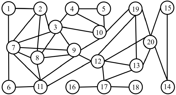
Figure 6: Network topology of the example WSNs.

The performance of the distributed algorithm based on the proposed M-MCKF algorithm (DM-MCKF) is compared with that of DKF, D-MCKF [36], and DMEEKF [39]. The state estimation performance is demonstrated by a classic WSNs example [15] with 20 sensor nodes, and the nodes and connections are illustrated in Fig. 6. All simulation conditions are set in the same way as in the simulation above. The simulation results and parameter settings are shown in Fig. 1b and Table III. Fig. 1b illustrates the instantaneous MSD of the DM-MCKF algorithm and several competitors in the second scenario, and the node number is $i=7$; Table III presents the steady-state MSD of the DM-MCKF, DMCKF, and DKF at nodes 7, 13, and 16, respectively. From simulation results, one can obtain that 1) the DM-MCKF algorithm performs best with mixed-Gaussian, Laplace, and $\alpha$-stable noise, and its performance is comparable to that of the DKF with Gaussian noise in terms of stead-state MSD, which demonstrates the robustness of the DM-MCKF algorithm; 2) for the same algorithm, the method performs better as more nodes are added that are next to it.

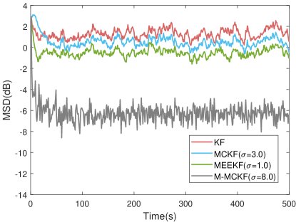
(a)

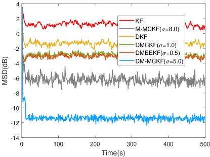
(b)

Figure 1: The validation of the proposed M-MCKF and DM-MCKF algorithms. (a) Comparison of the performance of the M-MCKF algorithm. (b) Comparison of the performance of the DM-MCKF algorithm.

TABLE II: The steady-state MSD (dB) comparison in different scenarios.

	First scenario		Second scenario		Third scenario		Fourth scenario
	MSD	$\sigma$	MSD	$\sigma$	MSD	$\sigma$	MSD	$\sigma$
KF	-7.66	N/A	1.24	N/A	1.83	N/A	5.91	N/A
MCKF	-7.63	30.0	0.34	3.0	1.59	4.0	4.68	2.5
R-MEEKF	-7.64	15.0	0.48	1.0	1.55	2.0	4.15	1.2
M-MCKF	-7.65	8.0	-6.23	8.0	1.36	3.5	2.19	3.0

TABLE III: The steady-state MSD (dB) of the distributed algorithms in different scenarios.

	First scenario		Second scenario		Third scenario		Fourth scenario
	MSD	$\sigma$	MSD	$\sigma$	MSD	$\sigma$	MSD	$\sigma$
KF	-7.66	N/A	1.24	N/A	0.34	N/A	5.90	N/A
M-MCKF	-7.65	8.0	-6.23	8.0	1.36	3.5	2.19	3.0
DKF($i=16$)	-9.08	N/A	0.52	N/A	0.91	N/A	N/A	N/A
DKF($i=13$)	-10.92	N/A	-0.61	N/A	-0.29	N/A	N/A	N/A
DKF($i=7$)	-12.0	N/A	-1.38	N/A	-0.81	N/A	N/A	N/A
DMCKF($i=16$)	-9.08	10.0	-0.94	1.0	0.57	2.0	3.22	2.0
DMCKF($i=13$)	-10.92	10.0	-2.18	1.0	-0.49	2.0	2.08	2.0
DMCKF($i=7$)	-12.0	10.0	-2.81	1.0	-1.07	2.0	1.82	2.0
DM-MCKF($i=16$)	-9.06	5.0	-8.21	5.0	0.36	3.0	1.67	2.5
DM-MCKF($i=13$)	-10.8	5.0	-10.36	5.0	-0.67	3.0	1.18	2.5
DM-MCKF($i=7$)	-11.89	5.0	-11.40	5.0	-1.21	3.0	0.91	2.5

IV-B Performance verification of the proposed algorithms considering packet drop

In addition, the state estimation performance is verified by the DM-MCKF-DPD, DMCKF-DPD, and stationary DKF algorithm [20] when applying them to a classic WSNs example [15] under data packet drop and impulsive noise conditions. It is assumed that the probability that all nodes can receive information from neighboring nodes is $p_{k}^{i,j}=0.8$, and the kernelwidths are shown in Fig. 2. The performance of the proposed algorithms is demonstrated with different nodes and different scenarios, and the corresponding results are shown in Fig. 2 and Table. Fig. 2a shows the convergence curves of MSD in the second scenario and the node number is $i=7$; Fig. 2b shows the convergence curves of MSD in the third scenario and the node number $i=13$. From Fig. 2, one can obtain that 1) the proposed DM-MCKF-DPD and DMCKF-DPD algorithms perform better than the DKF-DPD algorithm with non-Gaussian noise; 2) DM-MCKF-DPD algorithm performs better than DMCKF-DPD algorithm.

In addition, the C-DM-MCKF-DPD algorithm is verified in this part. The kernelwidth is set to 5.0 and the consensus coefficient is set as $\eta=0.05$. The convergence curve of MSD of the $17$th node in the second scenario is shown in Fig. 3a. From the simulation result, one can obtain that the consensus scheme ameliorates the impact of communication data loss to some extent.

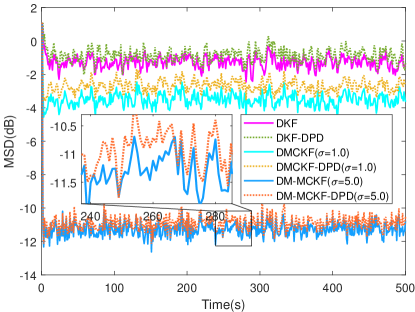
(a)

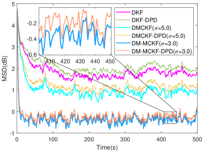
(b)

Figure 2: The performance of the DM-MCKF-DPD algorithm in different scenarios. (a) The convergence curves in the second scenario. (b) The convergence curves in the third scenario.

IV-C Parameters discussion

The influence of $\sigma$ on the performance of the M-MCKF and DM-MCKF algorithms is studied in this part. The influence of the consensus coefficient $\eta$ on the performance of the consensus DM-MCKF-DPD algorithm is investigated. The conclusions obtained can be used to guide the choice of the proposed algorithms.

The parameter $\sigma$ is set as $\sigma{\text{ = 3}}{\text{.0, 5}}{\text{.0, 8}}{\text{.0, 10}}{\text{.0, 15}}{\text{.0, 20}}{\text{.0, 35}}{\text{.0, 45}}{\text{.0}}$, and the initial states of the system are the same as in (128). The simulation results are presented in Fig. 4, Table IV, and Table V. Fig. 4 displays the convergence curves of the M-MCKF and DM-MCKF algorithms with different $\sigma$, respectively. The steady-state MSD, in the four scenarios, of the M-MCKF algorithm with different $\sigma$ is presented in Table IV. The steady-state MSD, in the four scenarios, of the DM-MCKF algorithm with different $\sigma$ and nodes is shown in Table V. From Fig. 4a and Table IV, one can obtain that the performance of the M-MCKF algorithm improves with the increasing $\sigma$ with Gaussian measurement noise, the it is optimal for mixed-Gaussian, Laplace, and $\alpha$-stable noise when $\sigma$ are around 8.0, 3.0, 3.0. From Fig. 4b and Table V, we can infer that the proposed DM-MCKF algorithm performs best with above the non-Gaussian noise when $\sigma$ is around 3.0. In addition, it is clear that the higher the number of neighboring nodes the better the performance of the DM-MCKF algorithm.

The parameter $\eta$ is set as $\eta{\text{ = }}0.1,{\text{ 0}}{\text{.2, 0}}{\text{.4, 0}}{\text{.48}}$, the kernelwidth of DM-MCKF-DPD and C-DM-MCKF-DPD are 3, and $p_{k}^{i,j}=0.9$. In the third scenario, the convergence curves of MSD of the $17$th node are displayed in Fig. 3b. In addition, the performance surfaces for the influence of the number of neighboring nodes ${\Omega_{i}}$ and the consensus coefficient $\eta$ on the performance of the C-DM-MCKF-DPD algorithm are shown in Fig. 5. From the simulation presented in Fig. 3b, one can obtain that the optimal consensus coefficient is around 0.2 for the $17$th node in the third scenario. From Fig. 5, one can obtain that 1) when the number of neighbors of a node ${\Omega_{i}}$ is small ($0<{\Omega_{i}}\leqslant 4$), choosing a larger consensus coefficient ($0.2\leqslant\eta\leqslant 0.35$) can improve the performance of the consensus algorithm; 2) when the number of neighbors of a node ${\Omega_{i}}$ is large ($4<{\Omega_{i}}\leqslant 7$), choosing a smaller consensus coefficient ($0.1\leqslant\eta\leqslant 0.2$) can improve the performance of the consensus algorithm.

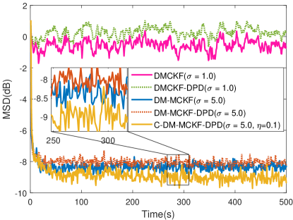
(a)

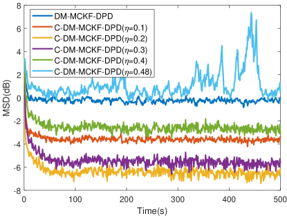
(b)

Figure 3: The performance comparison and analysis of consensus strategy. (a) The performance comparison of consensus strategy. (b) The consensus strategy with different $\eta$.

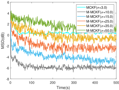
(a)

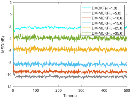
(b)

Figure 4: The performance analysis of the proposed algorithms with different kernelwidths. (a) The M-MCKF algorithm with different $\sigma$ in the second scenario. (b) The DM-MCKF algorithm with different $\sigma$.

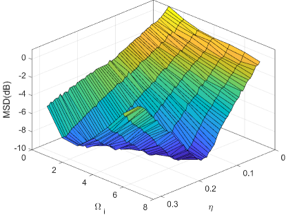
(a)

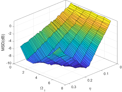
(b)

Figure 5: The performance surfaces with respect to parameter $\eta$ and ${\Omega_{i}}$. (a) The performance surface in the third scenario. (b) The performance surface in the fourth scenario.

TABLE IV: The steady-state MSD (dB) of M-MCKF algorithm with different $\sigma$.

	$\sigma=2$	$\sigma=3$	$\sigma=5$	$\sigma=8$	$\sigma=10$	$\sigma=15$	$\sigma=20$	$\sigma=35$	$\sigma=45$
First scenario	8.14	5.99	-7.52	-7.62	-7.63	-7.64	-7.64	-7.64	-7.64
Second scenario	20.98	14.56	10.32	-6.35	-5.90	-4.71	-3.47	-0.49	0.70
Third scenario	1.81	1.35	1.48	1.77	1.86	1.97	2.18	2.24	2.26
Fourth scenario	2.68	2.12	2.23	2.42	2.59	2.92	3.12	3.74	3.96

TABLE V: The steady-state MSD (dB) of the DM-MCKF algorithm with different $\sigma$.

	$\sigma=2$	$\sigma=3$	$\sigma=5$	$\sigma=8$	$\sigma=10$	$\sigma=15$	$\sigma=20$	$\sigma=35$	$\sigma=45$
First scenario(i=16)	4.82	-8.94	-8.99	-9.00	-9.00	-9.00	-9.00	-9.00	-9.00
First scenario(i=13)	2.63	-10.80	-10.84	-10.85	-10.85	-10.85	-10.85	-10.85	-10.85
First scenario(i=7)	-1.04	-11.78	-11.89	-11.99	-11.99	-11.99	-11.99	-11.99	-11.99
Second scenario(i=16)	14.65	-8.40	-8.23	-7.49	-6.98	-5.51	-4.33	-1.25	-0.10
Second scenario(i=13)	10.37	-10.45	-10.37	-9.98	-9.56	-8.30	-6.94	-3.89	-2.54
Second scenario(i=7)	9.92	-11.43	-11.42	-11.02	-10.62	-9.38	-8.14	-5.10	-3.70
Third scenario (i=16)	1.34	0.53	0.66	0.88	1.06	1.21	1.25	1.33	1.36
Third scenario(i=13)	0.40	-0.67	-0.43	-0.07	0.01	0.21	0.26	0.31	0.34
Third scenario(i=7)	-0.16	-1.21	-1.01	-0.78	-0.55	-0.46	-0.37	-0.32	0.22
Fourth scenario(i=16)	2.07	1.72	1.89	2.12	2.13	2.64	2.68	3.03	3.48
Fourth scenario(i=13)	1.62	1.11	1.23	1.41	1.42	1.74	1.88	2.36	2.62
Fourth scenario(i=7)	1.30	0.91	1.01	1.08	1.22	1.43	1.62	2.04	2.28

V Conclusion

The distributed state estimation over wireless sensor network with presence of non-Gaussian noise was concerned in this paper. By proposed a generalized packet drop model, the process of packet loss due to DoS attacks and energy limitations is described. A modified maximum correntropy KF algorithm was developed by analysing the advantages and disadvantages of existing algorithms, and it was extended to distributed M-MCKF algorithm. In addition, the distributed modified maximum correntropy Kalman filter incorporating the proposed generalized packet drop model was developed. The computational complexity of the DM-MCKF-DPD algorithm was demonstrated to be moderate compared to that of the conventional stationary DKF, and a sufficient condition to ensure the convergence of the fixed-point iterative algorithm was presented. Finally, simulations conducted with a 20-node WSNs demonstrated that the proposed DM-MCKF and DM-MCKF-DPD algorithms perform better than some existing algorithms. As future work, we intend to investigate the state estimation performance of a distributed Kalman filter based on the MEE criterion for WSNs under data packet drop conditions to further improve estimated performance with data packet drop and non-Gaussian noise.

Jiacheng He received the B.S. degree in mechanical engineering from University of Electronic Science and Technology of China, Chengdu, China, in 2020. He is currently pursuing a Ph.D. degree in the School of Mechanical and Electrical Engineering, University of Electronic Science and Technology of China, Chengdu, China. His current research interests include information-theoretic learning, signal processing, and target tracking.

Bei Peng received the B.S. degree in mechanical engineering from Beihang University, Beijing, China, in 1999, and the M.S. and Ph.D. degrees in mechanical engineering from Northwestern University, Evanston, IL, USA, in 2003 and 2008, respectively. He is currently a Full Professor of Mechanical Engineering with the University of Electronic Science and Technology of China, Chengdu, China. He holds 30 authorized patents. He has served as a PI or a CoPI for more than ten research projects, including the National Science Foundation of China. His research interests mainly include intelligent manufacturing systems, robotics, and its applications.

Zhenyu Feng was born in Anhui, China. He received the B.E. and MA.Sc degree from the University of Electronic Science and Technology of China, Chengdu, China, in 2014 and 2018, respectively. He is currently working toward the Ph.D. degree in the school of Mechanical and Electrical Engineering at University of Electronic Science and Technology of China. He has over five years of industrial experience in designing and implementing for applications in multi-agent sensor network systems. His current research interests lie in the field of multi-agent systems, underwater unmanned vehicle swarm intelligence, as well as distributed communication technology.

Xuemei Mao received the B.S. degree in mechanical design, manufacturing, and automation from Xidian University, Xian, China, in 2020. She is currently pursuing the Ph.D. degree in mechanical engineering with School of Mechanical and Electrical Engineering, University of Electronic Science and Technology of China, Chengdu, China. Her current research interests include signal processing, adaptive filtering, and target tracking.

Song Gao received the B.S. degree in mechanical design, manufacturing and automation from University of Electronic Science and Technology of China (UESTC), in 2020. He is currently pursuing the Ph.D. degree in mechanical engineering with School of Mechanical and Electrical Engineering of UESTC, Chengdu, China. His current research interests include multi-agent systems, consensus control, signal processing.

Gang Wang received the B.E. degree in Communication Engineering and the Ph.D. degree in Biomedical Engineering from University of Electronic Science and Technology of China, Chengdu, China, in 1999 and 2008, respectively. In 2009, he joined the School of Information and Communication Engineering, University of Electronic Science and Technology of China, China, where he is currently an Associate Professor. His current research interests include signal processing and intelligent systems.

References

• [1] Lien-Wu Chen and Jun-Xian Liu. Mobile crowdsourced guiding and finding with precise target positioning based on internet-of-things localization. IEEE Transactions on Systems, Man, and Cybernetics: Systems, 52(8):4849–4861, 2022.
• [2] Xiao-Lei Wang and Guang-Hong Yang. Distributed event-triggered $h_{\infty}$ filtering for discrete-time t–s fuzzy systems over sensor networks. IEEE Transactions on Systems, Man, and Cybernetics: Systems, 50(9):3269–3280, 2020.
• [3] L. Cheng, Y. Li, M. Xue, and Y. Wang. An indoor localization algorithm based on modified joint probabilistic data association for wireless sensor network. IEEE Transactions on Industrial Informatics, 17(1):63–72, 2021.
• [4] Xin Zhang, Bo He, Shuang Gao, Pengcheng Mu, Junchao Xu, and Ning Zhai. Multiple model auv navigation methodology with adaptivity and robustness. Ocean Engineering, 254:111258, 2022.
• [5] Qiaoling Zhang, Zhe Chen, and Fuliang Yin. Speaker tracking based on distributed particle filter in distributed microphone networks. IEEE Transactions on Systems, Man, and Cybernetics: Systems, 47(9):2433–2443, 2017.
• [6] Cong Huang, Weiping Ding, Ruifeng Gao, Peng Mei, and Hamid Reza Karimi. Distributed state-of-charge estimation for lithium-ion batteries with random sensor failure under dynamic event-triggering protocol. Information Fusion, 95:293–305, 2023.
• [7] Wen Yang, Guanrong Chen, Xiaofan Wang, and Ling Shi. Stochastic sensor activation for distributed state estimation over a sensor network. Automatica, 50(8):2070–2076, 2014.
• [8] Qinyuan Liu, Zidong Wang, Xiao He, and Dong-Hua Zhou. Event-based distributed filtering with stochastic measurement fading. IEEE Transactions on Industrial Informatics, 11(6):1643–1652, 2015.
• [9] Aquib Mustafa, Majid Mazouchi, and Hamidreza Modares. Secure event-triggered distributed kalman filters for state estimation over wireless sensor networks. IEEE Transactions on Systems, Man, and Cybernetics: Systems, 53(2):1268–1283, 2023.
• [10] Cong Huang and Bo Shen. Event-based fusion estimation for multi-rate systems subject to sensor degradations. Journal of the Franklin Institute, 358(16):8754–8771, 2021.
• [11] Xiaohua Ge, Qing-Long Han, and Zidong Wang. A dynamic event-triggered transmission scheme for distributed set-membership estimation over wireless sensor networks. IEEE Transactions on Cybernetics, 49(1):171–183, 2019.
• [12] Jia Guo, Dongyu Li, and Bo He. Intelligent collaborative navigation and control for auv tracking. IEEE Transactions on Industrial Informatics, 17(3):1732–1741, 2020.
• [13] Hongjiu Yang, Shuang Ju, Yuanqing Xia, and Jinhui Zhang. Predictive cloud control for networked multiagent systems with quantized signals under dos attacks. IEEE Transactions on Systems, Man, and Cybernetics: Systems, 51(2):1345–1353, 2021.
• [14] Bosen Lian, Yan Wan, Ya Zhang, Mushuang Liu, Frank L. Lewis, and Tianyou Chai. Distributed kalman consensus filter for estimation with moving targets. IEEE Transactions on Cybernetics, 52(6):5242–5254, 2022.
• [15] F. S. Cattivelli and A. H. Sayed. Diffusion strategies for distributed kalman filtering and smoothing. IEEE Transactions on Automatic Control, 55(9):2069–2084, 2010.
• [16] Wenling Li, Yingmin Jia, Junping Du, and Deyuan Meng. Diffusion kalman filter for distributed estimation with intermittent observations. In 2015 American Control Conference (ACC), pages 4455–4460, 2015.
• [17] G. Wang, N. Li, and Y. Zhang. Diffusion nonlinear kalman filter with intermittent observations. Proceedings of the Institution of Mechanical Engineers, 232(15):2775–2783, 2018.
• [18] Hao Chen, Jianan Wang, Chunyan Wang, Jiayuan Shan, and Ming Xin. Distributed diffusion unscented kalman filtering based on covariance intersection with intermittent measurements. Automatica, 132:109769, 2021.
• [19] Wenling Li, Yingmin Jia, and Junping Du. Distributed kalman consensus filter with intermittent observations. Journal of the Franklin Institute, 352(9):3764–3781, 2015. Special Issue on Synchronizability, Controllability and Observability of Networked Multi-Agent Systems.
• [20] Jianming Zhou, Guoxiang Gu, and Xiang Chen. Distributed kalman filtering over wireless sensor networks in the presence of data packet drops. IEEE Transactions on Automatic Control, 64(4):1603–1610, 2019.
• [21] Qingke Tan, Xiwang Dong, Fei Liu, Qingdong Li, and Zhang Ren. Weighted average consensus-based cubature information filtering for mobile sensor networks with intermittent observations. In 2017 36th Chinese Control Conference (CCC), pages 8946–8951, 2017.
• [22] Wen Yang, Chao Yang, Hongbo Shi, Ling Shi, and Guanrong Chen. Stochastic link activation for distributed filtering under sensor power constraint. Automatica, 75:109–118, 2017.
• [23] Bo Chen, Daniel W. C. Ho, Wen-An Zhang, and Li Yu. Distributed dimensionality reduction fusion estimation for cyber-physical systems under dos attacks. IEEE Transactions on Systems, Man, and Cybernetics: Systems, 49(2):455–468, 2019.
• [24] Jing Ma and Shuli Sun. Distributed fusion filter for networked stochastic uncertain systems with transmission delays and packet dropouts. Signal Processing, 130:268–278, 2017.
• [25] Tian Tian, Shuli Sun, and Na Li. Multi-sensor information fusion estimators for stochastic uncertain systems with correlated noises. Information Fusion, 27:126–137, 2016.
• [26] R. Caballero-Águila, A. Hermoso-Carazo, and J. Linares-Pérez. Distributed fusion filters from uncertain measured outputs in sensor networks with random packet losses. Information Fusion, 34:70–79, 2017.
• [27] Wei Yao and Sun Shu-Li. Recursive distributed fusion estimation for multi-sensor systems with missing measurements, multiple random transmission delays and packet losses. Signal Processing, 204:108829, 2023.
• [28] Jian Ding, Shuli Sun, Jing Ma, and Na Li. Fusion estimation for multi-sensor networked systems with packet loss compensation. Information Fusion, 45:138–149, 2019.
• [29] Jiacheng He, Gang Wang, Huijun Yu, JunMing Liu, and Bei Peng. Generalized minimum error entropy kalman filter for non-gaussian noise. ISA Transactions, 2022.
• [30] Hongwei Wang, Hongbin Li, Wei Zhang, Junyi Zuo, and Heping Wang. Maximum correntropy derivative-free robust Kalman filter and smoother. IEEE Access, 6:70794–70807, 2018.
• [31] Hongwei Wang, Hongbin Li, Wei Zhang, Junyi Zuo, and Heping Wang. Derivative-free Huber-Kalman smoothing based on alternating minimization. Signal Processing, 163:115–122, 2019.
• [32] Xuxiang Fan, Gang Wang, Jiachen Han, and Yinghui Wang. A background-impulse kalman filter with non-gaussian measurement noises. IEEE Transactions on Systems, Man, and Cybernetics: Systems, 53(4):2434–2443, 2023.
• [33] Jiacheng He, Gang Wang, Xi Zhang, Hongwei Wang, and Bei Peng. Maximum total generalized correntropy adaptive filtering for parameter estimation. Signal Processing, 203:108787, 2023.
• [34] Dongbing Gu. Distributed particle filter for target tracking. In Proceedings 2007 IEEE International Conference on Robotics and Automation, pages 3856–3861. IEEE, 2007.
• [35] Huajin Tang and Haizhou Li. Information theoretic learning: Reny’s entropy and kernel perspectives (Principe, j.; 2010) [book review]. IEEE Computational Intelligence Magazine, 6(3):60–62, 2011.
• [36] Gang Wang, Rui Xue, and Jinxin Wang. A distributed maximum correntropy kalman filter. Signal Processing, 160:247–251, 2019.
• [37] Chen Hu and Badong Chen. An efficient distributed kalman filter over sensor networks with maximum correntropy criterion. IEEE Transactions on Signal and Information Processing over Networks, 8:433–444, 2022.
• [38] Guoqing Wang, Ning Li, and Yonggang Zhang. Distributed maximum correntropy linear and nonlinear filters for systems with non-gaussian noises. Signal Processing, 182:107937, 2021.
• [39] Zhenyu Feng, Gang Wang, Bei Peng, Jiacheng He, and Kun Zhang. Distributed minimum error entropy kalman filter. Information Fusion, 91:556–565, 2023.
• [40] Yilin Mo, Sean Weerakkody, and Bruno Sinopoli. Physical authentication of control systems: Designing watermarked control inputs to detect counterfeit sensor outputs. IEEE Control Systems Magazine, 35(1):93–109, 2015.
• [41] Ziyang Guo, Dawei Shi, Karl Henrik Johansson, and Ling Shi. Optimal linear cyber-attack on remote state estimation. IEEE Transactions on Control of Network Systems, 4(1):4–13, 2016.
• [42] Weifeng Liu, Puskal P Pokharel, and José C Príncipe. Correntropy: Properties and applications in non-gaussian signal processing. IEEE Transactions on Signal Processing, 55(11):5286–5298, 2007.
• [43] Badong Chen, Xi Liu, Haiquan Zhao, and Jose C Principe. Maximum correntropy kalman filter. Automatica, 76:70–77, 2017.
• [44] Christopher M Bishop and Nasser M Nasrabadi. Pattern recognition and machine learning. Springer, 2006.
• [45] Christopher D Karlgaard. Nonlinear regression Huber–Kalman filtering and fixed-interval smoothing. Journal of guidance, control, and dynamics, 38(2):322–330, 2015.
• [46] Jiacheng He, Gang Wang, Bei Peng, Qi Sun, Zhenyu Feng, and Kun Zhang. Mixture quantized error entropy for recursive least squares adaptive filtering. Journal of the Franklin Institute, 359(3):1362–1381, 2022.
• [47] Jiacheng He, Gang Wang, Kui Cao, He Diao, Guotai Wang, and Bei Peng. Generalized minimum error entropy for robust learning. Pattern Recognition, 135:109188, 2023.
• [48] Gang Wang, Badong Chen, Xinyue Yang, Bei Peng, and Zhenyu Feng. Numerically stable minimum error entropy kalman filter. Signal Processing, 181:107914, 2021.