Continual Learning in Open-vocabulary Classification with Complementary Memory Systems

Abstract

We introduce a method for flexible and efficient continual learning in open-vocabulary image classification, drawing inspiration from the complementary learning systems observed in human cognition. Specifically, we propose to combine predictions from a CLIP zero-shot model and the exemplar-based model, using the zero-shot estimated probability that a sample’s class is within the exemplar classes. We also propose a “tree probe” method, an adaption of lazy learning principles, which enables fast learning from new examples with competitive accuracy to batch-trained linear models. We test in data incremental, class incremental, and task incremental settings, as well as ability to perform flexible inference on varying subsets of zero-shot and learned categories. Our proposed method achieves a good balance of learning speed, target task effectiveness, and zero-shot effectiveness. Code will be available here.

1 Introduction

A major machine learning goal is to create flexible learning systems, which we investigate in the context of image classification, with the following goals:

• Flexible inference: classify an image within any label set, testable via zero-shot classification

• Continual improvement: accuracy improves as new data is received for related tasks without detriment to previous tasks

• Efficient incremental learning: can efficiently update the model with new training examples

Flexible inference and continual improvement lead to robust and widely usable systems. Efficient incremental learning reduces cost of training and facilitates responsive and interactive learning approaches.

To our knowledge, no solution exists that meets all these goals. Open vocabulary methods, such as CLIP (Radford et al., 2021), attain flexible inference but cannot easily learn and improve with new examples. Continual learning methods, such as LwF (Li & Hoiem, 2018), iCaRL (Rebuffi et al., 2017), EWC (Kirkpatrick et al., 2016), and GDumb (Prabhu et al., 2020), lack flexible inference and are not easily extended to open vocabulary models. For example, LwF requires maintaining classification heads for previous tasks and GDumb maintains examples for every possible label; neither strategy directly applies when the label set is unbounded. In fact, one homogeneous system cannot easily accommodate all goals. A deep network can aggregate information over enormous datasets to achieve flexible inference, but updates from small targeted subsets can disrupt other tasks. Instance-based methods can incrementally learn and continually improve, but cannot generalize to novel labels.

To build such a flexible learning system, we are inspired by the flexibility of human learning and inference, enabled by complementary learning systems (CLS) (O’Reilly et al., 2014). The fast-learning system forms new memories and associations with sparse connections, enabling non-disruptive storage of individual experiences. The slow-learning system gradually consolidates information in a densely connected network, encoding general knowledge and regularities across experiences. The interplay between these two complementary systems enables the brain to balance the rapid encoding of novel information and gradual generalization of knowledge. How can we make computer learning systems that likewise benefit from both consolidated and exemplar-based memory systems to continually learn with zero-shot inference ability?

Our system likewise comprises three components: slow-learning system, fast-learning system, and the association module that incorporates both models for prediction. In this work, we focus on the latter two components. We investigate in the context of open-vocabulary image classification, using CLIP as the slow-learning system. Our fast-learning system stores individual representations of learning exemplars, and the challenge is to learn from them in a way that is performant in both accuracy and learning time (Sec. 3.2). To balance speed and performance, we consider classic learning approaches. One option is linear probe, which can achieve good accuracy but learns from a new example in $\mathcal{O}(n)$ time, where $n$ represents the total number of exemplars. K-nearest neighbor (KNN) can learn in $\mathcal{O}(1)$ time but tends to be less accurate than linear probe. Based on local linear models from the lazy learning literature (Bontempi et al., 1999), we propose a “tree probe” method that hierarchically clusters examples and trains linear models for each cluster. The time to learn from a new example is $\mathcal{O}(\rm{log}~{}n)$ (in practice, essentially constant time), and the accuracy is close to linear probe.

A second challenge is to predict using both CLIP and exemplar models (Sec. 3.3) to achieve good performance on new tasks while maintaining zero-shot performance. The exemplar model tends to perform well for test samples with labels that are in the exemplar set (“exemplar covered”), while the consolidated model can potentially predict any label. At test time, we may not know whether the label of a given test image is exemplar-covered. Our idea is to use CLIP to estimate the probability that an image’s label is exemplar-covered and then weight the predictions of the two models.

Our complementary system achieves good accuracy, efficient learning, and flexible inference. We evaluate our method in the forms of data-incremental, class-incremental, and task-incremental learning, as well as flexible inference with categorization tasks that involve some, all, or none of the exemplar-covered labels. Additionally, we compare on a recently created external benchmark (Zheng et al., 2023), outperforming all compared approaches with the additional benefit of efficient learning. In summary, the reader may benefit from the following paper contributions:

• Tree-probe exemplar model: Our locally linear models using a hierarchical clustering can be considered a member of the long-studied lazy learning approaches (Bontempi et al., 1999), but we are not aware of this specific method being proposed or used. Tree-probe has practically constant training time in number of training samples and achieves better accuracy than KNN approaches. This is attractive for interactive search, active learning, and other applications where annotated examples are received in a trickle and fast learning is required.

• Exemplar and consolidated model combination with embeddings: Our approach, to use the consolidated model to estimate applicability of the exemplar model and to combine model predictions in the label embedding space, enables effective continual open-vocabulary learning and performs significantly better than alternatives we tested.

• Flexible learning/inference: Our experimental setup evaluates both the ability to continually learn from new samples and to flexibly apply those learnings to various category sets. This may provide a useful test framework to further improve open-vocabulary continual learning.

2 Related works

2.1 Instance-based learning (IBL)

Instance-based learning (IBL) (Aggarwal, 2014) is a family of learning algorithms that construct a decision boundary using a memory of training instances, allowing for efficient and flexible adaptation to new data points. This learning paradigm relies on the principle of local approximation, where predictions are made based on the stored instances that are most similar to the query. One of the most well-known IBL methods is the $k$-Nearest Neighbors (KNN) algorithm, which has been extensively studied for its simplicity and effectiveness in various domains, including classification and regression tasks (Guo et al., 2003; Zhang et al., 2006; 2017; Song et al., 2017).

Closely related to IBL is lazy learning, in which training data is organized for prediction at inference time instead of training time. This approach can be more practical than batch or “eager” learning in applications like online recommendation systems, when the training data is constantly evolving. Lazy learning approaches can include KNN or locally linear regression (Atkeson et al., 1997) or classification models (Aggarwal, 2014), where models are trained based on neighbors to the query.

We investigate KNN, a form of locally linear classifiers, and globally linear classifiers, exploring their trade-offs for training and inference time and accuracy on a growing set of exemplars, as well as how to combine their predictions with a static image-language foundation model.

2.2 Open-vocabulary image classification

Open-vocabulary image classification aims to categorize images without constraints of predefined labels. CLIP (Radford et al., 2021) achieves this by learning embedding spaces of images and text, trained via a contrastive objective that corresponding image/text pairs will be more similar than non-corresponding pairs. A new image can be classified into an arbitrary set of labels based on the similarity of the image embedding features to the text embedding features corresponding to each label. An alternative approach is to jointly encode the image and text information and decode into text. Following this approach, vision-language models, such as GPV-1 (Gupta et al., 2022), GPV-2 (Kamath et al., 2022), VL-BERT (Su et al., 2020), VL-T5 (Cho et al., 2021), Unified-IO (Lu et al., 2022), Gato (Reed et al., 2022), and Flamingo (Alayrac et al., 2022), can solve a broad range of tasks that includes open-vocabulary image classification, but typically are larger and more complex than CLIP. We use CLIP as our consolidated model, due to its simplicity and verified effectiveness in a broad range of tasks (Wortsman et al., 2022b; Gu et al., 2021; Ghiasi et al., 2021; Lin et al., 2022).

2.3 Continual learning

Continual learning techniques aim to acquire new knowledge over time while preserving previously learned knowledge (McCloskey & Cohen, 1989). Approaches to continual learning can be broadly categorized into regularization (Li & Hoiem, 2016; Kirkpatrick et al., 2016; Zenke et al., 2017), parameter isolation (Aljundi et al., 2017; Rusu et al., 2016; Serrà et al., 2018; Mallya & Lazebnik, 2018; Zhang et al., 2020), and rehearsal methods (Rebuffi et al., 2017; Yan et al., 2021; Lopez-Paz & Ranzato, 2017; Shin et al., 2017). Regularization techniques generally impose constraints on the learning process to alleviate forgetting. Parameter isolation methods maintain learning stability by fixing subsets of parameters (Mallya & Lazebnik, 2018; Serrà et al., 2018) or extending model with new parameters (Rusu et al., 2016; Yoon et al., 2017; Zhang et al., 2020). Rehearsal methods involve storing and replaying past data samples during training (Shin et al., 2017; Bang et al., 2021). We are not aware of many works that address continual learning in the context of open-vocabulary image classification. WiSE-FT (Wortsman et al., 2022a) finetunes CLIP encoders on target tasks and averages finetuned weights with original weights for robustness to distribution shifts. Likewise, CLS-ER (Arani et al., 2022) exponentially averages model weights in different paces for its plastic and stable model to balance learning and forgetting, drawing inspirations from CLS. Though not specifically designed for open-vocabulary continual learning, WiSE-FT and CLS-ER can be modified to counter forgetting. Recently, ZSCL (Zheng et al., 2023) explores this setting but mainly focuses on finetuning consolidated CLIP encoders. It combines LwF (Li & Hoiem, 2016) and a weight ensemble idea similar to WiSE-FT as the remedy to reduce forgetting during finetuning. Rather than refining or expanding a single model, our approach is to create a separate exemplar-based model that complements a pre-trained and non-updated more general consolidated model. In our tree-probe method, the exemplar-based model continually learns using a local rehearsal, such that incorporating a new example requires only storing the new image and text embeddings and tuning a linear model using a subset of visually similar examples. This requires little storage or computation and preserves the generality of the consolidated model.

3 Method

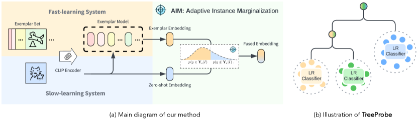
Figure 1: Method overview. (a) Our model integrates rapid and slow-learning systems. Final results are made by fusing the predictions from both systems using AIM. (b) Illustration of TreeProbe, which incrementally adds and hierarchically clusters examples. TreeProbe trains logistic regression classifiers using examples in updated leaf nodes.

Given an image $I$ and label set $Y$, our system’s inference task is to assign the correct label $y\in Y$. Each training example (or “exemplar”) consists of an image, and a ground-truth label. Our problem setting is called “open-vocabulary” or “zero-shot”, as the labels can be represented and related through text, and the task at inference time may contain labels or candidate label sets not observed during training. The training goal is to efficiently update the model with each new example, such that accuracy improves for related labels while maintaining zero-shot performance.

Analogous to complimentary learning systems (CLS) theory (O’Reilly et al., 2014), our approach (Fig. 1) uses two models: a CLIP image/text encoder as the consolidated slow learning system (Sec. 3.1), and a rapid-learning exemplar-based model that stores and encodes image and label embeddings (Sec. 3.2). The CLIP model can assign confidence to any label from an arbitrary set. The exemplar-based model can acquire expertise that complements the CLIP model, but its scope is limited to exemplar labels. In Sec. 3.3, we propose simple mechanisms to combine the predictions of each model to retain zero-shot capability while improving in tasks related to received examples.

3.1 Slow-learning system: zero-shot model

Deep networks, such as CLIP (Radford et al., 2021), relate to slow-learning systems in humans in that they repeatedly process examples to iteratively consolidate experience and improve predictive ability in dense weight connections. We use CLIP as the slow-learning consolidated system, taking advantage of its representations and open-vocabulary predictive ability learned from batch training on massive datasets. To preserve generality, we do not update the CLIP parameters and instead train complementary exemplar-based models to be used in combination with CLIP.

CLIP encodes an input image $I$ using an image encoder $f_{\text{img}}$ to an image embedding $\mathbf{v}_{I}=f_{\text{img}}(I)$, and encodes an input collection of text labels $T={t_{1},t_{2},\dots,t_{m}}$ using a text encoder $f_{\text{txt}}$ to text embeddings $\mathbf{v}_{t_{i}}=f_{\text{txt}}(t_{i})$. Following (Radford et al., 2021), a text label $t_{i}$ is framed as a sentence or caption contextualizing the image label $y_{i}$, such as “a photo of a F-16, a style of aircraft” to represent the image label “F-16” in an airplane classification task. The model computes logits for each label as cosine similarity between the image and text label, weighted by temperature $\tau$ (=100 in CLIP):

$$l(\mathbf{v}_{I},\mathbf{v}_{t_{i}})=\tau\cdot\frac{\mathbf{v}_{I}\cdot\mathbf{v}_{t_{i}}}{|v_{I}||v_{t_{i}}|}.$$ (1)

Logits can be converted to probabilities using a softmax function:

$$p_{z}(y=y_{i}|I)=\frac{\exp(l(\mathbf{v}_{I},\mathbf{v}_{t_{i}}))}{\sum_{j=1}^{m}\exp(l(\mathbf{v}_{I},\mathbf{v}_{t_{j}})}).$$ (2)

The label with maximum probability is predicted.

3.2 Fast-learning system: exemplar-based model

For the fast-learning system, given one or more exemplars, our goal is to maximize classification performance with minimal training time and acceptable inference time. We consider two approaches: instance-based and model-based prediction. Instance-based prediction leverages the exemplar set directly by retrieving and comparing samples. Model-based prediction seeks to capture the underlying structure of the data through a parameterized model. In both cases, our approach leverages the embeddings from CLIP encoders to reduce storage and improve sample efficiency of learning.

Our exemplar memory module $M$ stores encoded image embeddings and their labels. Each entry in the memory can be denoted by $M_{j}=\{\mathbf{v}_{I_{j}},y_{j}\}$ where $j$ represents the entry index, $\mathbf{v}_{I_{j}}$ represents the image embedding of $I_{j}$, and $y_{j}$ is the corresponding label.

Given a set of target labels, the exemplar-based model can produce a probability for each label $p_{e}(y=y_{i}|\mathbf{v}_{I})$. Alternatively, the prediction can be represented as an embedding vector $\mathbf{v}_{e}$ of composition of one or several text embeddings. Prediction in terms of $\mathbf{v}_{e}$ enables the exemplar model to support zero-shot prediction for labels similar to exemplar labels.

KNN: Given $\mathbf{v}_{I}$, the KNN memory module finds its most similar $k$ entries in the memory through cosine similarities between $\mathbf{v}_{I}$ and all $\mathbf{v}_{I_{j}}$ in the memory. Let $\mathcal{N}_{k}(\mathbf{v}_{I})$ be the set of indices of the $k$ highest cosine similarity scores to $\mathbf{v}_{I}$. KNN classification for $\mathbf{v}_{I}$ can be performed by majority voting from the values: $\hat{y}=\arg\max_{y}\sum_{j\in\mathcal{N}_{k}(\mathbf{v}_{I})}\mathds{1}(y_{j}=y).$ Here, $\mathds{1}(\cdot)$ is an indicator function. The probability of $\mathbf{v}_{I}$ being label $y_{i}$ is $p_{e}(y=y_{i}|\mathbf{v}_{I})=\frac{1}{k}\sum_{j\in\mathcal{N}_{k}(\mathbf{v}_{I})}\mathds{1}(y_{j}=y_{i})$.

To predict the embedding $\mathbf{v}_{e}$, we can use the text embedding of the most likely label. But we find that computing a similarity-weighted average of the retrieved text embeddings gives better performance: $\mathbf{v}_{e}=\sum_{j\in\mathcal{N}_{k}(\mathbf{v}_{I})}\beta_{j}\cdot f_{\text{txt}}(t_{j})$, where $\beta_{j}=\frac{\exp(l(\mathbf{v}_{I},\mathbf{v}_{I_{j}}))}{\sum_{j^{\prime}\in\mathcal{N}_{k}(\mathbf{v}_{I})}\exp(l(\mathbf{v}_{I},e_{\mathbf{v}_{j^{\prime}}}))}$.

KNN takes virtually no time to train ($\mathcal{O}(1)$), and reasonably fast retrieval is possible with optimized libraries and parallel computing. However, accuracy tends to be lower than model-based methods.

Linear probe: Parameterized models offer an alternative approach, learning a fixed set of parameters that exploit the underlying structures of the data to maximize classification performance. When new exemplars are added, the linear probe (LinProbe) method is to extract image embeddings and train linear classifiers on all accumulated exemplars. This relates to GDumb (Prabhu et al., 2020), a simple experience replay method that retrains models from scratch each time new data is received. But, since we do not have the CLIP training data and wish to enable fast learning and retain zero-shot ability, we do not retrain or fine-tune the CLIP encoders. The output probability can be written as: $p_{e}(y=y_{i}|\mathbf{v}_{I};\bm{\theta})=\frac{\exp{(\bm{\theta}_{y_{i}}^{T}\mathbf{v}_{I})}}{\sum_{y_{j}\in\mathbf{\mathbf{Y}_{e}}}\exp{(\bm{\theta}_{y_{j}}^{T}\mathbf{v}_{I})}},$ where $\bm{\theta}_{y_{i}}$ represents the learned model parameters for label $y_{i}$ and $\mathbf{Y}_{e}$ is the union of exemplar labels. The predicted embedding is the text embedding of the label $\hat{y}$ with maximum probability: $\mathbf{v}_{e}=f_{\text{txt}}(t_{\hat{y}})$.

Compared to KNN, the LinProbe model is much slower to train — $\mathcal{O}(n)$ for $n$ training samples assuming a constant number of epochs, which may be prohibitive when the model needs to be updated quickly based on few examples. However, classification accuracy tends to be higher.

Tree probe: In a continual learning setting, we would ideally have fast training time of KNN with the relatively good accuracy of LinProbe. We take inspiration from the instance-based and lazy learning literature (Aggarwal, 2014), particularly locally linear models (Domeniconi & Gunopulos, 2002; Atkeson et al., 1997). These methods classify a test sample by finding its $k$-nearest neighbors and applying a linear classifier trained on the neighbors. This achieves $\mathcal{O}(1)$ training time but may be impractical for inference, since a new classifier may need to be trained for each test sample.

Instead, we propose an approximation, building a clustering tree from the training data and training a linear classifier in each leaf node. Starting from a root node, we search for the nearest leaf node for a new data point and insert it if the node has not reached the predefined node capacity $\psi$. If a leaf node reaches $\psi$, it splits into two child nodes and becomes a non-leaf node. The attached data points are distributed to their children by KMeans clustering. In experiments, when receiving new data, samples are added into the cluster tree one by one. Only classifiers in affected leaf node(s) need to be retrained. When fixing the number of linear model training epochs and KMeans iterations, the complexity to incorporate a new exemplar in training is $\mathcal{O}(\psi+\log~{}n)$ with $\psi>>\log~{}n$; the training time stays limited even when the total number of exemplars is very large.

The simplest inference method would be to assign a test sample to a leaf node in the cluster tree and classify it within the corresponding linear model, but this may lead to non-smooth predictions for samples near the cluster boundaries. In our experiments, we ensemble the classifiers from leaf nodes corresponding to the $k$ nearest neighbors, such that the final output probability $p_{e}(y=y_{i}|\mathbf{v}_{I})$ is the average of the probabilities predicted by each neighbor’s classifier.

Similar to KNN, the exemplar embedding $\mathbf{v}_{e}$ can be computed as the text embedding of the most likely label from all neighbor classifiers. However, we obtain the best performance using a similarity-weighted average embedding from the most likely label $\hat{y}_{k}$ of each classifier in the retrieval set: $\mathbf{v}_{e}=\sum_{k}\beta_{k}\cdot f_{\text{txt}}(t_{\hat{y}_{k}})$, where $\beta_{k}\propto\exp(l(\mathbf{v}_{I},\mathbf{v}_{I_{k}}))$ and $\mathbf{v}_{I_{k}}$ is the image embedding the $k$th neighbor. The tree-probe method, denoted TreeProbe, achieves similar accuracy to LinProbe in our continual learning experiments with sufficiently large $\psi$, but with much faster training time.

3.3 Fusing predictions of the two models

We want to integrate predictions from the zero-shot and exemplar-based models to retain good open-vocabulary classification performance and improve accuracy in predicting exemplar labels. This can be tricky, especially when some labels in the task are not contained within the exemplar labels.

One approach is to simply average the probability or embedding predictions of the two models:

$$p(y=y_{i}|I)=\alpha p_{e}(y=y_{i}|\mathbf{v}_{I})+(1-\alpha)p_{z}(y=y_{i}|I)$$ (3)

$$\mathbf{v}_{\text{out}}=\alpha\mathbf{v}_{e}+(1-\alpha)\mathbf{v}_{I}$$ (4)

The label probability is computed from $\mathbf{v}_{\text{out}}$ using $l(\mathbf{v}_{\text{out}},\mathbf{v}_{t_{i}})$, as in Eqs. 1 and 2. When setting $\alpha=0.5$ for an unweighted average, this approach is denoted as Avg-Prob or Avg-Emb, respectively. Using an unweighted average presumes that the zero-shot and exemplar models are equally reliable for all samples. However, if the test sample’s label is within the exemplar’s domain, the exemplar model will tend to be more accurate; otherwise, the zero-shot model will almost certainly outperform. The test label is unknown, but an educated guess could enable a better prediction.

Addressing this issue, we devise an adaptive weighting mechanism, named Adaptive Instance Marginalization (AIM), that estimates the likelihood of a test sample’s label being in the exemplar set and balances the predictions from both models accordingly. The target label set is divided into exemplar $y\in\mathbf{Y}_{e}$ and non-exemplar $y\notin\mathbf{Y}_{e}$ subsets, where $\mathbf{Y}_{e}$ is the union of all exemplar labels.

The likelihoods $p(y\in\mathbf{Y}_{e}|I)$ and $p(y\notin\mathbf{Y}_{e}|I)$ are obtained by summing the zero-shot probabilities over these subsets: $p(y\in\mathbf{Y}_{e}|I)=\sum_{i\in\mathbf{Y}_{e}}p_{z}(y=y_{i}|I)$ and $p(y\notin\mathbf{Y}_{e}|I)=\sum_{i\notin\mathbf{Y}_{e}}p_{z}(y=y_{i}|I)=1-p(y_{i}\in\mathbf{Y}_{e}|I)$, with the summation in the denominator of Eq. 2 over all candidate labels for the current task. Our AIM-Emb method sets $\alpha=p(y\in\mathbf{Y}_{e}|I)$ in Eq. 4.

Our AIM-Prob method encodes that both zero-shot and exemplar models are predictive for exemplar classes, while only the zero-shot model can be trusted for non-exemplar classes:

$$p(y=y_{i}|I)=p(y\in\mathbf{Y}_{e}|I)\frac{p_{z}(y=y_{i}|I)p_{e}(y=y_{i}|\mathbf{v}_{I})}{\sum_{j\in\mathbf{Y}_{e}}p_{z}(y=y_{j}|I)p_{e}(y=y_{j}|\mathbf{v}_{I})}+p(y\notin\mathbf{Y}_{e}|I)p_{z}(y=y_{i}|I).$$ (5)

The AIM method capitalizes on the strengths of both models, improving overall performance.

4 Experimental Setup

4.1 Tasks

We evaluate our system on target and zero-shot classification tasks. A “task” is an assignment of an image into a label from particular label set. The exemplar model has received examples in the context of “target” tasks but not “zero-shot” tasks. We utilize general tasks such as ImageNet (Russakovsky et al., 2015), SUN397 (Xiao et al., 2010), CIFAR100 (Krizhevsky & Hinton, 2009), and fine-grained tasks like EuroSAT (Helber et al., 2019), OxfordIIITPets (Parkhi et al., 2012), DTD (Cimpoi et al., 2014), Flower102 (Nilsback & Zisserman, 2008), FGVCAircraft (Maji et al., 2013), StanfordCars (Krause et al., 2013), Food101 (Bossard et al., 2014), UCF101 (Soomro et al., 2012).

We report main results using target tasks CIFAR100, SUN397, FGVCAircraft, EuroSAT, OxfordIIITPets, StanfordCars, Food101 and Flowers102 and zero-shot tasks ImageNet, UCF101, and DTD. The supplemental material contains dataset descriptions, prompt templates, zero-shot performance of tasks, and additional experimental results and analysis.

4.2 Evaluation scenarios

We consider several continual learning scenarios for receiving data: 1) Data incremental: A fraction of the training data, randomly sampled without enforcing class balance, is added in each stage; 2) Class incremental: All training data for a randomly sampled subset of classes are added in each stage; 3) Task incremental: All data for a single task, i.e. a dataset of examples assigned to a set of target labels, are added in each stage. Data incremental learning includes seven stages, comprising 2%, 4%, 8%, 16%, 32%, 64%, and 100% of task data, respectively. Class incremental learning divides a task into five stages, each containing 20% of classes. In task incremental learning, each task is considered a stage. In data and class incremental experiments, models are built separately for each target task. A target task is fully evaluated if there is at least one training sample for that task, even if there are no training samples for some classes. In task incremental, one model is built spanning all accumulated labels in each stage. In all cases, results are reported as the average accuracy of target and zero-shot tasks at each stage. We additionally compute the averaged accuracy on seen classes and unseen classes of each target task for class incremental learning to give more detailed result analysis.

Flexible inference: In the task incremental setting, after all training data for target tasks is received, we will evaluate each method’s performance in three inference scenarios:

• Zero-shot: evaluate on each zero-shot task and then average the accuracy on all tasks.

• Union + Zero-shot: we first create a union of target task labels that is considered as candidate labels for each target task. Then, we randomly sample 100 labels from the union of zero-shot task labels. We separately compute the average accuracies on the target and zero-shot tasks. The final performance is the average of the target and zero-shot accuracy.

• Mix + Zero-shot: we randomly split the union of target labels into five splits. For each split, we additionally add a random sample of 100 labels from the zero-shot task. To balance evaluation across classes, we draw 100 test samples per class. Performance is the average across all splits.

These scenarios are especially challenging for most continual learning methods because there is no task identifier at inference time, and the label of a test sample will sometimes be among the trained classes and sometimes not.

5 Experimental Results

5.1 Effectiveness of complementary system and AIM

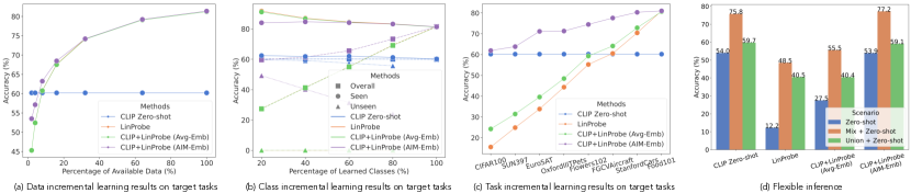
Figure 2: (a) Results comparing CLIP zero-shot, LinProbe and CLIP+LinProbe with Avg-Emb and AIM-Emb on target tasks under the data incremental learning scenario. (b) Results of corresponding models on target tasks under class incremental learning. We visualize curves for seen and unseen classes including the overall performance identified with different markers. (c) Results of corresponding models on target tasks under task incremental learning. (d) Flexible inference results after task incremental learning on all tasks. Note LinProbe is hard to see in (a) and (b) because it has similar results as CLIP+LinProbe (Avg-Emb).

We first investigate the importance of complementary learning systems and the effectiveness of AIM. We design experiments comparing CLIP Zero-shot model, exemplar model using LinProbe  and then complementary models that incorporate CLIP Zero-shot and LinProbe using the Avg-Emb and AIM-Emb fusing operations, denoted by CLIP+LinProb (Avg-Emb) and CLIP+LinProbe (AIM-Emb).

The results on target tasks under data, class, and task incremental learning scenario are shown in Fig. 2 (a-c). For data incremental, except for CLIP zero-shot, all other methods constantly improve on target tasks, with CLIP+LinProbe (AIM-Emb) being the best on all stages. When the percentage of available data is larger than 20%, all other models surpass the zero-shot model. LinProbe and CLIP+LinProbe (Avg-Emb) have similar performances on target tasks, which can also be observed in the class incremental learning results in Fig. 2 (b).

Results under the class incremental learning are important since they simulate the case that the exemplar labels do not cover some labels in the task. In this case, we cannot simply choose whether to use the exemplar model or zero-shot model for prediction by contrasting if exemplar labels totally overlap with candidate labels. In Fig. 2 (b), we plot the accuracies on seen and unseen classes along with the overall accuracy on all classes. The zero-shot model is inferior to other methods in seen classes but performs well in unseen classes. LinProbe has good accuracy on seen classes, but its unseen accuracies are close to 0. Likewise for CLIP+LinProbe (Avg-Emb). The AIM-Emb version has a slightly lower accuracy than the Avg-Emb version on seen classes of early stages ($<$60% classes) but has reasonable performance on unseen classes, especially in earlier stages. Its unseen accuracy drops with more learned classes because AIM gradually tends to give more confidence for the exemplar model. In all, we still see the overall accuracy of CLIP+LinProbe (AIM-Emb) is the best among all methods, demonstrating the efficacy of AIM.

From the results in Fig. 2 (c) under the task-incremental learning scenario, the AIM approach steadily shows better performance than the zero-shot model at all stages. LinProbe and CLIP+LinProbe (Avg-Emb) can only beat the zero-shot model after the 6-th stage (FGVCAircraft). Both versions of CLIP+LinProbe show better performance than exemplar-only models, demonstrating the benefits of complementary systems.

The flexible inference scenarios highlight the effectiveness of the CLIP zero-shot model, as shown in Fig. 2 (d). Since exemplar-only models entirely bias towards learned classes, they are incompetent on zero-shot tasks. Hence, LinProbe has poor results in all scenarios. However, CLIP+LinProbe (Avg-Emb) shows a considerable improvement over LinProbe on Zero-shot and Mix+Zero-shot scenarios while being comparable on Union+Zero-shot. When substituting the fusing operation with AIM-Emb, the performances of all scenarios significantly improve, with Mix+Zero-shot even slightly better than the CLIP zero-shot model. Overall, AIM achieves similar flexible inference performance to the CLIP zero-shot model.

5.2 Comparison of Efficiency and Accuracy for Fast-Learning Approaches

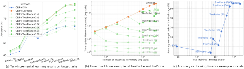
Figure 3: (a) Results of different complementary models under the task-incremental learning scenario. Numbers included in a bracket are the node capacity of corresponding TreeProbe models. (b) We perform an efficiency analysis of TreeProbe with different node capacities and LinProbe by estimating how much time needed to incorporate one example into the exemplar model with different number of instances carried in the exemplar set.To minimize randomness, each method is run five times. At each data collection point, we sample an example from the exemplar set and fit it to memory five times. Thus, each data point averages 25 unique simulations. $x$ and $y$-axes are visualized in log scale. (c) The accuracies of different complementary models on target tasks after learning the final stage ($y$-axis) vs. the total training time in log scale ($x$-axis).

In this part, we perform a thorough analysis of different complementary models using AIM on their performances and efficiency: CLIP+KNN, CLIP+LinProbe and CLIP+TreeProbe. We can also vary the node capacities of TreeProbe to create different versions of CLIP+TreeProbe models.

We compare their performance under the task incremental learning scenario. Results in Fig. 3 (a) show that node capacity can be used to control the performance of CLIP+TreeProbe. When node capacity is larger than 5k, TreeProbe steadily outperforms KNN, and when node capacity reaches 100k, TreeProbe is slightly better than LinProbe. Fig. 3 (b) shows that LinProbe conforms to linear learning complexity as the number of instances in the exemplar set. When node capacity is not reached, TreeProbe is the same as LinProbe since TreeProbe has only one leaf node and one classifier. After reaching the node capacity, TreeProbe shows constant learning complexity. TreeProbe (100k) and (50k) achieve similar performance to LinProbe but with 6x and 25x improvement in learning speed when the exemplar set contains $>$ 220k samples. This confirms our analysis of the time complexity of learning for different exemplar models in Sec. 3.2. Fig. 3 (c) combines the results of Fig. 3 (a) and Fig. 3 (b), showing the trade-off of learning efficiency and accuracy. The TreeProbe method, thus, provides flexibility to choose the node capacity that appropriately balances responsiveness with performance for a given application.

5.3 Comparison to previous methods

Method Transfer $\triangle$ Avg. $\triangle$ Last $\triangle$ CLIP Zero-shot 69.4 0.0 65.3 0.0 65.3 0.0 LwF (Li & Hoiem, 2016) 56.9 -12.5 64.7 -0.6 74.6 +9.3 iCaRL (Rebuffi et al., 2017) 50.4 -19.0 65.7 +0.4 80.1 +14.8 WiSE-FT (Wortsman et al., 2022a) 52.3 -17.1 60.7 -4.6 77.7 +12.4 ZSCL (Zheng et al., 2023) 68.1 -1.3 75.4 +10.1 83.6 +18.3 TreeProbe (50k) 69.3 -0.1 75.9 +10.6 85.5 +20.2

Table 1: Comparison of different methods on MTIL in Order I from ZSCL (Zheng et al., 2023). All results are taken from other ZSCL’s paper except for TreeProbe. “Transfer” evaluates the model’s performance on zero-shot tasks; “Last” is the averaged accuracy on all target tasks after finishing the final task while “Avg.” computes the average task performance on all training stages.

As introduced in Sec. 2.3, ZSCL (Zheng et al., 2023) explores a similar setting to open-vocabulary continual learning and is mainly evaluated under the task-incremental learning scenario. To keep the comparison as fair as possible, we evaluate our approach under their evaluation protocols, and we utilize the same prompt ensemble technique, data split ratio and seed, backbone network (ViT-B/16), etc. The result is in Tab. 1. Our TreeProbe (50k) model achieves the best performance under all metrics. Compared to the CLIP zero-shot model, our method barely compromises on Transfer, showing that our approach maintains robust performance on zero-shot tasks. It is also noteworthy that our method is more lightweight than ZSCL in GPU consumption, and we do not perform hyperparameter selection for each task as we assume we have no knowledge about future tasks, whereas ZSCL used different learning rates for different tasks for better performance.

5.4 Scaling to larger zero-shot models

Method ViT-B/32 ViT-L/14@336px ViT-H/14 Target Zero-shot Target Zero-shot Target Zero-shot CLIP Zero-shot 60.2 54.0 72.1 65.6 79.2 71.7 TreeProbe (50k) 80.5 53.8 86.6 65.4 90.2 71.6

Table 2: Accuracies on target and zero-shot tasks with pretrained encoders of different capacities.

We use the CLIP ViT/B-32 model as our default zero-shot model but can easily adapt to other models. We experiment with the pre-trained CLIP model ViT-L/14@336px, which boasts approximately 4x the capacity of ViT-B/32, and ViT-H/14, which is double the size of ViT-L/14@336px. We present our findings in Tab. 2, where both methods are evaluated under the task incremental learning scenario. Performance increases for larger models, and TreeProbe consistently outperforms CLIP Zero-shot on the target tasks with nearly identical performance on zero-shot tasks, demonstrating that our approach is beneficial for a wide range of zero-shot model sizes.

6 Conclusion and limitations

In this work, we present an efficient and performant “tree probe” exemplar-based model and Adaptive Instance Marginalization to combine zero-shot and exemplar models for open-vocabulary continual learning. Our method is able to efficiently incorporate new samples, improving performance for related tasks without negatively impacting zero-shot task performance, providing a simple way to continually improve large-scale pretrained image-text classification models. We believe this work is a step towards more flexible, efficient, and effective strategies in open-vocabulary continual learning.

Our work has several limitations. First, we do not consider constraints in how many exemplars can be stored. Since each exemplar requires storing up to 4KB for the image and text encodings (using the base CLIP ViT-B/32 model without any compression or limiting precision), roughly one million exemplars can be stored per 4GB of memory. Second, we do not investigate how to improve the consolidated zero-shot model. This is a promising direction for future work. Finally, we do not explore structured prediction problems like semantic segmentation or visual question answering, which likely require more complex image representations than a single embedding vector.

Acknowledgements: This work is supported in part by ONR award N00014-21-1-2705, ONR award N00014-23-1-2383, and U.S. DARPA ECOLE Program No. #HR00112390060. The views and conclusions contained herein are those of the authors and should not be interpreted as necessarily representing the official policies, either expressed or implied, of DARPA, ONR, or the U.S. Government. The U.S. Government is authorized to reproduce and distribute reprints for governmental purposes notwithstanding any copyright annotation therein.

Supplemental Materials: Continual Learning in Open-vocabulary Classification with Complementary Memory Systems

S-1 Algorithmic descriptions of TreeProbe 

Input: Training set $X$, Tree $T$, Leaf capacity $\psi$

Output: Trained classifiers in each leaf node of $T$ foreach $\mathbf{v}_{i}\in X$ do

       $l$ = NearestLeaf($\mathbf{v}_{i}$, $T$)

       if Count($l$) $<$ $\psi$ then

             $l$ = InsertData($\mathbf{v}_{i}$, $l$)

             TrainClassifier($l$)

       end if

      else

             SplitNode($l$, $\mathbf{v}_{i}$)

             $l$ = NearestLeaf($\mathbf{v}_{i}$, $T$)

             $l$ = InsertData($\mathbf{v}_{i}$, $l$)

             TrainClassifier($l$)

       end if

      

end foreach

Algorithm 1 Training Procedure of TreeProbe 

Input: Image embedding $\mathbf{v}_{I}$, Tree $T$, Number of nearest nodes $k$, Exemplar set $M$,

Output: Exemplar embedding $\mathbf{v}_{e}$ for $\mathbf{v}_{I}$ $\mathbf{v}_{\mathcal{K}}$ = FindNearestSamples($\mathbf{v}_{I}$, $M$)

$\mathbf{v}$ = list()

foreach $\mathbf{v}_{i}\in\mathbf{v}_{\mathcal{K}}$ do

       $l$ = NearestLeaf($\mathbf{v}_{i}$, $T$)

       $c$ = GetClassifier($l$)

       $\mathbf{v}$ $\leftarrow$ Classify($\mathbf{v}_{I}$, $c$)

end foreach

$\mathbf{v}_{e}$ = ComputeEmbedding($\mathbf{v}$, $\mathbf{v}_{I}$)

Algorithm 2 Inference Procedure of TreeProbe 

Algorithm 1 and Algorithm 2 contain psuedocode for the training and inference of our TreeProbe method. Definitions of the involved functions are provided below:

• NearestLeaf($\mathbf{v}_{i}$, $T$): Returns the nearest leaf node to the data point $x_{i}$ in tree $T$.

• Count($l$): Returns the current number of data points in leaf node $l$.

• InsertData($\mathbf{v}_{i}$, $l$): Inserts data point $\mathbf{v}_{i}$ into leaf node $l$ and returns the updated node.

• SplitNode($l$, $\mathbf{v}_{i}$): Splits leaf node $l$ into two child nodes when it reaches capacity, distributes data points using KMeans clustering, and adds new data point $\mathbf{v}_{i}$ to the appropriate child node.

• TrainClassifier($l$): Trains a linear classifier on the data points in leaf node $l$.

• FindNearestSamples($\mathbf{v}_{I}$, $M$): Finds the $k$ nearest neighbors in the exemplar set to the image embedding $\mathbf{v}_{I}$.

• GetClassifier($l$): Return the classifier for node $l$.

• Classify($\mathbf{v}_{i}$, $c$): Classifies $\mathbf{v}_{i}$ using the linear classifier $c$, returning the label embedding of the most likely label.

• ComputeEmbedding($\mathbf{v}$, $\mathbf{v}_{I}$): Computes the exemplar embedding for $\mathbf{v}_{I}$ by applying a similarity-weighted average of the text embeddings of the most likely class labels from a temporal list $\mathbf{v}$.

The notation of Algorithm 1 and Algorithm 2 may differ from the main paper.

S-2 Implementation details

We conduct our experiments on a setup featuring an RTX 3090 GPU and an AMD Ryzen 9 5950X CPU, using PyTorch as our primary framework. We adhere to the CLIP code example, using sklearn LogisticRegression to implement linear classifiers and setting the sklearn regularization strength to 0.316. The maximum iteration is set to 5k. Our tree probe’s node capacity is set at 50k. For efficient retrieval from large-scale exemplar sets, we use FAISS (Johnson et al., 2019), specifically using the IndexFlatIP class for its precision and performance. Model performances are gauged via Top-1 accuracy, with the officially released ViT-B/32 CLIP checkpoint serving as our memory or zero-shot model. We select $k=9$ based on a hyperparameter sweep. Our approach is not sensitive to $k$, with very similar performance in a range from 6 to 30.

S-3 More experiment setting details

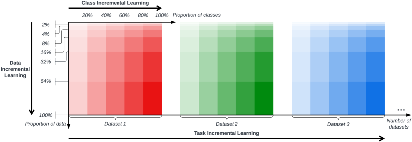
Figure S1: Illustration of continual learning scenarios. Data incremental learning includes seven stages, each comprising 2%, 4%, 8%, 16%, 32%, 64%, and 100% of task data respectively. Class incremental learning divides a task into five stages, each containing 20% of classes. In task incremental learning, each task is considered a stage.

We present an illustration of data, class, and task incremental learning scenarios in Fig. S1. When evaluating different methods in data and class incremental learning scenarios, we ensure fairness by randomly selecting an identical portion of data/class for all methods, achieved by setting the same seed. Models are separately built for each target task. The performance of each stage is averaged across all target tasks. In task-incremental learning, each stage is embodied by a distinct task. The task order is randomly arranged as CIFAR100, SUN397, FGVCAircraft, EuroSAT, OxfordIIITPets, StanfordCars, Food101, and Flowers102, consistent for all methods for fair comparison. As shown in ZSCL (Zheng et al., 2023), task order has little impact on the relative performance comparison of different models. For all learning scenarios, we make the assumption that training data accumulates across all stages in all scenarios, with a similar spirit to (Prabhu et al., 2023). This assumption is based on the fact that real-world applications are often more limited by computational and time budgets than by storage. If data privacy is not a concern, building a continual learning system without losing data access is more effective than assuming past data is non-accessible. Furthermore, we enhance storage efficiency by saving samples as condensed feature vectors, a significant improvement over some earlier works.

S-4 Descriptions of tasks

We perform experiments on various commonly used visual datasets to demonstrate the generalization capabilities of our method. These datasets encompass a broad range of image categories and application scenarios, including both fine-grained and generalized datasets. We briefly introduce all used tasks in this paper in the following.

S-4.1 General tasks

ImageNet ImageNet (Russakovsky et al., 2015) contains 1,281,167 training images, 50,000 validation images and 100,000 test images. The categories represent a wide variety of objects, animals, scenes, and even abstract concepts. This dataset has served as a fundamental dataset to evaluate performances of classification models, or as a pretraining dataset.

CIFAR100 The CIFAR100 dataset (Krizhevsky & Hinton, 2009) consists of object images and is a subset of the 80 million tiny images dataset. It contains 60,000 32$\times$32 color images from 100 object categories, with 600 images per category. The dataset has 100 fine-grained classes, grouped into 20 coarse-grained classes.

SUN397 The SUN397 dataset (Xiao et al., 2010) consists of scene images, containing 108,754 images across 397 scene categories, with each category having between 100 and 500 images. This dataset is commonly used for scene understanding tasks. Since there is no official dataset split for this dataset, we randomly select 60% of images as training data, 20% as validation data, and the rest as test data. We use NumPy random permutation to split with the seed set to 0.

S-4.2 Fine-grained tasks

FGVCAircraft The FGVCAircraft dataset (Maji et al., 2013) serves as a benchmark for fine-grained visual categorization of aircraft. It contains 10,200 images from 102 distinct categories. Each category includes approximately 100 images, annotated with the aircraft model, variant, and manufacturer.

DTD The Describable Textures Dataset (DTD) (Cimpoi et al., 2014) consists of 5,640 images across 47 texture categories, with each category featuring 120 real-world texture images such as fabrics, rocks, and surfaces. The dataset poses a challenge for texture classification due to subtle differences between textures within the same category and large variations in texture appearance caused by scale, orientation, and lighting.

Food101 The Food-101 dataset (Bossard et al., 2014) comprises 101,000 images across 101 food categories, each with 1,000 images. This dataset challenges fine-grained image classification due to high intra-class variation and visual similarities across categories. It serves as a rigorous benchmark for evaluating computer vision models in food recognition and provides a robust platform for training machine learning models in understanding culinary aesthetics and preferences.

StanfordCars The StanfordCars dataset (Krause et al., 2013) is a benchmark dataset containing 16,185 images from 196 different car classes, divided into a 50-50 training and testing split. The classes correspond to specific car makes, models, and years, such as the 2012 Tesla Model S or 2012 BMW M3 coupe.

Flowers102 The 102 Category Flower Dataset (Nilsback & Zisserman, 2008) is a compilation of flower images. It includes 8,189 images across 102 flower categories, with each category containing between 40 and 258 images. The dataset’s images vary in size and aspect ratio, captured using different cameras, lighting conditions, and backgrounds.

OxfordIIITPets The OxfordIIITPets dataset (Parkhi et al., 2012) is a collection of pet images, featuring 7,349 images from 37 different cat and dog breeds. Each breed has between 100 and 200 images. The dataset is challenging because the appearance of the same breed can vary significantly, and different breeds may have similar-looking features.

EuroSAT The EuroSAT dataset (Helber et al., 2019) is a remote sensing image dataset comprising Sentinel-2 satellite data. It contains 27,000 images that cover 13 spectral bands and consist of 10 different land use and land cover categories, including forests, urban areas, and water bodies. This dataset is commonly employed for remote sensing and land cover classification tasks. Since there is no official dataset split for this dataset, we randomly select 70% of images as training data and the rest as validation data. We use NumPy random permutation to perform splitting with the seed set to 0.

UCF101 The UCF101 dataset (Soomro et al., 2012) is a commonly used benchmark for action recognition. It consists of 13,320 videos from 101 action categories, with each category containing at least 100 videos. The actions include a wide range of human activities such as basketball shooting, horse riding, and juggling. The dataset is unique in its focus on complex, naturalistic action sequences, with videos varying in length from a few seconds to a minute. Since there is no official dataset split for this dataset, we randomly select 70% of images as training data and the rest as validation data. We use NumPy random permutation to perform splitting with the seed set to 0.

S-4.3 Long-tailed task

Places365LT Places365LT (Liu et al., 2019) a synthetic long-tail derivative of Places2 dataset (Zhou et al., 2018). The image resolution is 256$\times$256. It contains 365 scene classes with at least 5 samples each. The classes are not uniformly distributed, forming a long-tailed distribution. It contains some label noises, making classification even harder on this dataset.

S-5 Prompt templates for tasks

Task(s) Prompt template ImageNet (Russakovsky et al., 2015), CIFAR100 (Krizhevsky & Hinton, 2009), SUN397 (Xiao et al., 2010) “a photo of a {label}.” FGVCAircraft (Maji et al., 2013) “a photo of a {label}, a type of aircraft.” DTD (Cimpoi et al., 2014) “a photo of a {label} texture.” StanfordCars (Krause et al., 2013) “a photo of a {label}, a type of car.” Food101 (Bossard et al., 2014) “a photo of {label}, a type of food.” Flowers102 (Nilsback & Zisserman, 2008) “a photo of a {label}, a type of flower.” OxfordIIITPets (Parkhi et al., 2012) “a photo of a {label}, a type of pet.” EuroSAT (Helber et al., 2019) “a centered satellite photo of {label}.” UCF101 (Parkhi et al., 2012) “a video of a person doing {label}.” Places365LT (Liu et al., 2019) “a photo of the {label}, a type of place.”

Table 1: Prompts of tasks

CLIP (Radford et al., 2021) suggests utilizing a sentence template (e.g., ‘‘A photo of a {label}.’’), as input to the text decoder instead of a plain text label, due to its training data being primarily full sentences describing images. Consistent with this paper’s focus, we employ a simple prompt template for each task. Most of these templates are based on CLIP’s recommendations and are summarized in Tab. 1.

S-6 Zero-shot performances on different tasks

Task	Zero-shot Acc (%)	Official ZS Acc (%)
ImageNet (Russakovsky et al., 2015)	59.7	63.2
CIFAR100 (Krizhevsky & Hinton, 2009)	62.3	65.1
SUN397 (Xiao et al., 2010)	59.2	63.2
FGVCAircraft (Maji et al., 2013)	18.1	21.2
DTD (Cimpoi et al., 2014)	42.0	44.5
StanfordCars (Krause et al., 2013)	58.6	59.4
Food101 (Bossard et al., 2014)	82.6	84.4
Flowers102 (Nilsback & Zisserman, 2008)	67.9	66.7
OxfordIIITPets (Parkhi et al., 2012)	87.5	87.0
EuroSAT (Helber et al., 2019)	45.4	49.4
UCF101 (Parkhi et al., 2012)	60.1	64.5
Places365LT (Liu et al., 2019)	40.0	/

Table 2: Zero-shot performances of CLIP ViT-B/32 pretrained model on different tasks. “ZS” is for zero-shot and “Acc” is for accuracy. Results of column “Official ZS Acc” are taken from the CLIP original paper (Radford et al., 2021). “/” represents lack of official results.

Tab. 2 shows the zero-shot performance of our implementation in different tasks. We conjecture that the main difference of official zero-shot performances comes from the ensemble prompt trick as mentioned in CLIP (Radford et al., 2021) and randomness in dataset splits of several tasks (e.g., SUN397).

S-7 Additional results

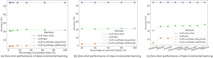
Figure S2: Zero-shot performances on data (a), class (b), and task (c) incremental learning scenarios. $x$-axis represents stages when the evaluation is performed.

S-7.1 Zero-shot task performances of every stage

We further append the results of zero-shot tasks evaluated after each stage on the data, class, and task incremental learning in Fig. S2. Across all scenarios, AIM-Emb helps maintain the zero-shot performances on all stages.

S-7.2 More results of the comparison to previous methods

Method Transfer $\triangle$ Avg. $\triangle$ Last $\triangle$ CLIP Zero-shot 69.4 0.0 65.3 0.0 65.3 0.0 LwF (Li & Hoiem, 2016) 56.9 -12.5 64.7 -0.6 74.6 +9.3 iCaRL (Rebuffi et al., 2017) 50.4 -19.0 65.7 +0.4 80.1 +14.8 WiSE-FT (Wortsman et al., 2022a) 52.3 -17.1 60.7 -4.6 77.7 +12.4 ZSCL (Zheng et al., 2023) 68.1 -1.3 75.4 +10.1 83.6 +18.3 KNN 69.3 -0.1 72.7 +7.4 78.4 +13.1 LinProbe 69.3 -0.1 77.1 +11.8 86.0 +20.7 TreeProbe (50k) 69.3 -0.1 75.9 +10.6 85.5 +20.2

Table 3: Comparison of different methods on MTIL in Order I from ZSCL (Zheng et al., 2023). KNN, LinProbe , and TreeProbe (50k) are complementary methods with AIM-Emb as the fusing approach.

	Aircraft	Caltech101	CIFAR100	DTD	EuroSAT	Flowers	Food	MNIST	OxfordPet	Cars	SUN397
Transfer		87.90	68.22	45.32	54.61	71.08	88.86	59.45	89.07	64.61	64.05	69.3
Aircraft	52.45	87.90	68.22	45.32	54.61	71.08	88.86	59.45	89.07	64.61	64.05
Caltech101	52.48	96.89	68.22	45.32	54.61	71.08	88.86	59.45	89.07	64.61	64.05
CIFAR100	52.48	96.89	68.22	45.32	54.61	71.08	88.86	59.45	89.07	64.61	64.05
DTD	52.42	96.83	81.98	70.32	54.61	71.08	88.86	59.45	89.07	64.61	64.05
EuroSAT	52.45	89.92	81.99	66.65	95.74	71.08	88.86	59.45	89.07	64.61	64.05
Flowers	52.51	90.55	81.93	66.44	95.74	54.12	88.86	59.45	89.07	64.61	64.05
Food	52.48	90.78	81.94	67.23	95.78	65.49	92.25	59.45	89.07	64.61	64.05
MNIST	52.09	93.95	81.96	69.73	94.33	95.69	92.27	98.59	89.07	64.61	64.05
OxfordPet	52.63	95.10	82.05	70.05	95.63	95.69	92.29	98.58	92.91	64.61	64.05
Cars	52.54	95.22	81.94	67.98	94.15	95.59	92.29	98.58	93.02	86.27	64.05
SUN397	52.48	95.56	81.94	66.91	95.59	95.59	92.21	98.60	93.19	86.15	81.76	85.5
Avg.	52.45	93.59	79.47	61.93	80.49	77.96	90.40	73.68	90.15	68.53	65.66	75.9

Table 4: Accuracy (%) of our TreeProbe (50k) model on the MTIL benchmark with order-I. Each row represents the performance on every dataset of the model trained after the corresponding task. Transfer, Avg., and Last metrics are shown in color. We follow the same table arrangement as in ZSCL (Zheng et al., 2023).

We also supplement the results obtained by KNN and LinProbe while comparing to previous methods in Tab. 3. As shown, all of the approaches of complementary systems with AIM-Emb achieve good Transfer, reiterating the effectiveness of AIM. LinProbe excels at all metrics with the cost of efficiency, which is predictable from the results shown in our main manuscript.

To give more details on the accuracies we achieve on every task under all stages for TreeProbe (50k), we follow ZSCL (Zheng et al., 2023) to give all numbers in Tab. 4 for further reference.

S-8 Additional ablation experiments

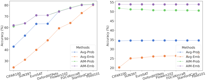
Figure S3: Target (left) and zero-shot (right) accuracies of different fusing operations.

Effect of different fusing operations. We describe several forms of the fusing operations in Sec. 3.3, including: Avg-Prob, AIM-Prob, Avg-Emb, and AIM-Emb. We compare using TreeProbe (50k) under the task incremental learning scenario. Fig. S3 shows the results on target and zero-shot tasks. The figure shows that AIM-Emb and AIM-Prob have similar performance on target tasks, surpassing the other two fusing operations. Combined with the zero-shot performance, the results suggest the effectiveness of AIM in adaptively choosing the better prediction model. The probabilistic prediction is better than the embedding prediction when performing averaging in both target tasks and zero-shot tasks. But when combined with AIM, the embedding version has a reasonably better performance in zero-shot tasks. Therefore, we choose AIM-Emb as the default fusing operation.

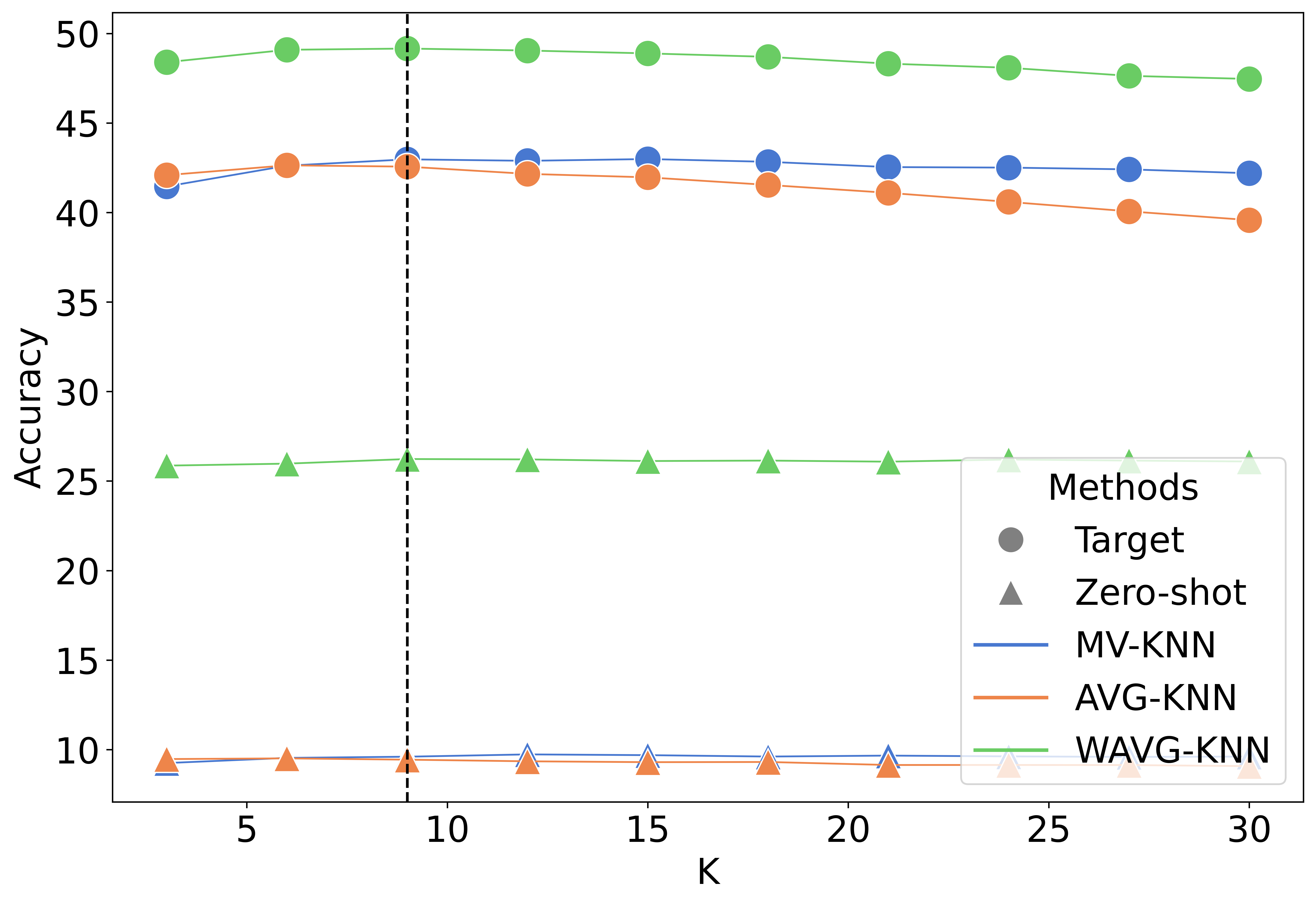
Figure S4: Results of different versions of KNN on target tasks after finishing all stages under the task incremental learning scenario. We further ablate on $k$ selection so choose $k$ as the $x$-axis. The vertical dashed line represents $k=9$.

Different versions of KNN and choice of $k$. As indicated in Sec. 3.2, we can get the embedding by taking the one attached to the most likely label (MV-KNN), or averaging the text embeddings of the $k$ nearest neighbors (AVG-KNN), or performing a weighted-averaging over the embeddings of all $k$ nearest neighbors where weights come from the similarities between the image embedding and the $k$ neighbors’ image embeddings (WAVG-KNN). We also compare these approaches under different $k$s to further choose a suitable $k$ for experiments. As indicated in Fig. S4, from the curve, $k=9$ gives reasonable performances of all approaches on both the target and zero-shot tasks. Compared to AVG-KNN, larger $k$ is more beneficial for MV-KNN since larger $k$ is more stable for MV-KNN, and it is more likely to include more mismatches from the nearest neighbors forAVG-KNN . From the plot, we can clearly read that WAVG-KNN is consistently better than AVG-KNN and MV-KNN across different $k$s, making it our default option of the prediction approach for fast learning system.

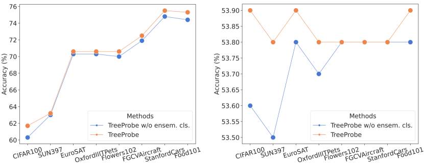
Figure S5: Target and zero-shot task performance comparison w.r.t. ensemble classifiers. “TreeProbe w/o ensem. cls.” is the version of TreeProbe by finding the cluster most similar to the input and using the corresponding classifier to predict labels. The reported accuracy is the average across tasks after incrementally receiving training data from the datasets shown on the $x$-axis.

Effect of ensemble classifiers in TreeProbe inference. Referencing Sec. 3.2, we observe that ensemble predictions from multiple classifiers associated with $k$ retrievals slightly enhance performance. Fig. S5 presents these results under the task incremental learning setting for eight target tasks. Our final model, TreeProbe, is better than its variant without the ensemble classification function in both target and zero-shot performance. The additional inference cost for ensemble predictions is negligible, so we choose it as the default setting for its better performance.

S-9 Evaluation on long-tailed classification

Method CLIP Zero-shot KNN LinProbe TreeProbe KNN* LinProbe* TreeProbe* PaCo RAC Accuracy (%) 40.0 35.5 37.0 30.5 40.4 42.7 41.3 41.2 47.2

Table 5: Comparison of long-tailed classification on Places365LT (Liu et al., 2019). * means + AIM-Emb. For this experiment, we use CLIP ViT-L/14@336px as the backbone network.

In long-tailed classification, some test labels are rare or unobserved in training, so blending exemplar-based models with consolidated models can be beneficial, as shown by (Long et al., 2022). To accommodate this setting, we adjust our AIM-Emb method by considering the 2/3 rarest labels as not being present in the exemplar set and the remainder as being present, to calculate $\mathbf{v}_{\text{out}}$. In this experiment, the node capacity of TreeProbe methods is 10k. In Tab. 5, we present results on the Places365LT dataset (Liu et al., 2019). Our AIM-Emb method with LinProbe and TreeProbe outperform the zero-shot baseline. We also compare to PaCo (Cui et al., 2021) and RAC (Long et al., 2022), which are specifically designed for long-tail classification. PaCo incorporates learnable class centers to account for class imbalance in a contrastive learning approach. RAC trains an image encoder augmented with label predictions from retrieved exemplars. Although not specifically designed for long-tailed classification, our method performs similar to PaCo, but RAC performs best of all.

References

- Aggarwal (2014) Charu C. Aggarwal. Instance-based learning : A survey. In Data Classification: Algorithms and Applications, chapter 6. CRC Press, 2014.
- Alayrac et al. (2022) Jean-Baptiste Alayrac, Jeff Donahue, Pauline Luc, Antoine Miech, Iain Barr, Yana Hasson, Karel Lenc, Arthur Mensch, Katie Millican, Malcolm Reynolds, Roman Ring, Eliza Rutherford, Serkan Cabi, Tengda Han, Zhitao Gong, Sina Samangooei, Marianne Monteiro, Jacob Menick, Sebastian Borgeaud, Andy Brock, Aida Nematzadeh, Sahand Sharifzadeh, Mikolaj Binkowski, Ricardo Barreira, Oriol Vinyals, Andrew Zisserman, and Karen Simonyan. Flamingo: a visual language model for few-shot learning. ArXiv, abs/2204.14198, 2022.
- Aljundi et al. (2017) Rahaf Aljundi, Punarjay Chakravarty, and Tinne Tuytelaars. Expert gate: Lifelong learning with a network of experts. In CVPR, pp. 7120–7129, 2017.
- Arani et al. (2022) Elahe Arani, Fahad Sarfraz, and Bahram Zonooz. Learning fast, learning slow: A general continual learning method based on complementary learning system. In ICLR, 2022.
- Atkeson et al. (1997) Christopher G. Atkeson, Andrew W. Moore, and Stefan Schaal. Locally weighted learning. Artificial Intelligence Review, 11:11–73, 1997.
- Bang et al. (2021) Jihwan Bang, Heesu Kim, Youngjoon Yoo, Jung-Woo Ha, and Jonghyun Choi. Rainbow memory: Continual learning with a memory of diverse samples. In CVPR, pp. 8218–8227, 2021.
- Bontempi et al. (1999) Gianluca Bontempi, Mauro Birattari, and Hugues Bersini. Lazy learning for local modelling and control design. International Journal of Control, 72(7-8):643–658, 1999.
- Bossard et al. (2014) Lukas Bossard, Matthieu Guillaumin, and Luc Van Gool. Food-101 – mining discriminative components with random forests. In European Conference on Computer Vision, 2014.
- Cho et al. (2021) Jaemin Cho, Jie Lei, Hao Tan, and Mohit Bansal. Unifying vision-and-language tasks via text generation. ArXiv, abs/2102.02779, 2021.
- Cimpoi et al. (2014) M. Cimpoi, S. Maji, I. Kokkinos, S. Mohamed, , and A. Vedaldi. Describing textures in the wild. In Proc. CVPR, 2014.
- Cui et al. (2021) Jiequan Cui, Zhisheng Zhong, Shu Liu, Bei Yu, and Jiaya Jia. Parametric contrastive learning. In ICCV, pp. 695–704, 2021.
- Domeniconi & Gunopulos (2002) C. Domeniconi and D. Gunopulos. Adaptive nearest neighbor classification using support vector machines. In NeurIPS, 2002.
- Ghiasi et al. (2021) Golnaz Ghiasi, Xiuye Gu, Yin Cui, and Tsung-Yi Lin. Open-vocabulary image segmentation. arXiv preprint arXiv:2112.12143, 2021.
- Gu et al. (2021) Xiuye Gu, Tsung-Yi Lin, Weicheng Kuo, and Yin Cui. Open-vocabulary object detection via vision and language knowledge distillation. arXiv preprint arXiv:2104.13921, 2021.
- Guo et al. (2003) Gongde Guo, Hui Wang, David Bell, Yaxin Bi, and Kieran Greer. Knn model-based approach in classification. In On The Move to Meaningful Internet Systems 2003: CoopIS, DOA, and ODBASE: OTM Confederated International Conferences, CoopIS, DOA, and ODBASE 2003, Catania, Sicily, Italy, November 3-7, 2003. Proceedings, pp. 986–996. Springer, 2003.
- Gupta et al. (2022) Tanmay Gupta, Amita Kamath, Aniruddha Kembhavi, and Derek Hoiem. Towards general purpose vision systems: An end-to-end task-agnostic vision-language architecture. In CVPR, 2022.
- Helber et al. (2019) Patrick Helber, Benjamin Bischke, Andreas Dengel, and Damian Borth. Eurosat: A novel dataset and deep learning benchmark for land use and land cover classification. IEEE Journal of Selected Topics in Applied Earth Observations and Remote Sensing, 2019.
- Johnson et al. (2019) Jeff Johnson, Matthijs Douze, and Hervé Jégou. Billion-scale similarity search with GPUs. IEEE Transactions on Big Data, 2019.
- Kamath et al. (2022) Amita Kamath, Christopher Clark, Tanmay Gupta, Eric Kolve, Derek Hoiem, and Aniruddha Kembhavi. Webly supervised concept expansion for general purpose vision models. In ECCV, 2022.
- Kirkpatrick et al. (2016) James Kirkpatrick, Razvan Pascanu, Neil C. Rabinowitz, Joel Veness, Guillaume Desjardins, Andrei A. Rusu, Kieran Milan, John Quan, Tiago Ramalho, Agnieszka Grabska-Barwinska, Demis Hassabis, Claudia Clopath, Dharshan Kumaran, and Raia Hadsell. Overcoming catastrophic forgetting in neural networks. CoRR, abs/1612.00796, 2016.
- Krause et al. (2013) Jonathan Krause, Michael Stark, Jia Deng, and Li Fei-Fei. 3d object representations for fine-grained categorization. In 4th International IEEE Workshop on 3D Representation and Recognition (3dRR-13), 2013.
- Krizhevsky & Hinton (2009) A. Krizhevsky and G. Hinton. Learning multiple layers of features from tiny images. Master’s thesis, Department of Computer Science, University of Toronto, 2009.
- Li & Hoiem (2018) Z. Li and D. Hoiem. Learning without forgetting. PAMI, 40(12):2935–2947, 2018.
- Li & Hoiem (2016) Zhizhong Li and Derek Hoiem. Learning without forgetting. In Proc. ECCV, 2016.
- Lin et al. (2022) Ziyi Lin, Shijie Geng, Renrui Zhang, Peng Gao, Gerard de Melo, Xiaogang Wang, Jifeng Dai, Yu Qiao, and Hongsheng Li. Frozen clip models are efficient video learners. In Computer Vision–ECCV 2022: 17th European Conference, Tel Aviv, Israel, October 23–27, 2022, Proceedings, Part XXXV, pp. 388–404. Springer, 2022.
- Liu et al. (2019) Ziwei Liu, Zhongqi Miao, Xiaohang Zhan, Jiayun Wang, Boqing Gong, and Stella X. Yu. Large-scale long-tailed recognition in an open world. In CVPR, pp. 2537–2546, 2019.
- Long et al. (2022) Alexander Long, Wei Yin, Thalaiyasingam Ajanthan, Vu Nguyen, Pulak Purkait, Ravi Garg, Alan Blair, Chunhua Shen, and Anton van den Hengel. Retrieval augmented classification for long-tail visual recognition. In Proc. CVPR, 2022.
- Lopez-Paz & Ranzato (2017) David Lopez-Paz and Marc’Aurelio Ranzato. Gradient episodic memory for continual learning. In Proc. NeurIPS, 2017.
- Lu et al. (2022) Jiasen Lu, Christopher Clark, Rowan Zellers, Roozbeh Mottaghi, and Aniruddha Kembhavi. Unified-io: A unified model for vision, language, and multi-modal tasks. ArXiv, abs/2206.08916, 2022.
- Maji et al. (2013) Subhransu Maji, Esa Rahtu, Juho Kannala, Matthew Blaschko, and Andrea Vedaldi. Fine-grained visual classification of aircraft. arXiv preprint arXiv:1306.5151, 2013.
- Mallya & Lazebnik (2018) Arun Mallya and Svetlana Lazebnik. Packnet: Adding multiple tasks to a single network by iterative pruning. In CVPR, 2018.
- McCloskey & Cohen (1989) Michael McCloskey and Neal J Cohen. Catastrophic interference in connectionist networks: The sequential learning problem. In Psychology of learning and motivation, volume 24, pp. 109–165. Elsevier, 1989.
- Nilsback & Zisserman (2008) Maria-Elena Nilsback and Andrew Zisserman. Automated flower classification over a large number of classes. In 2008 Sixth Indian Conference on Computer Vision, Graphics & Image Processing, 2008.
- O’Reilly et al. (2014) Randall C. O’Reilly, Rajan Bhattacharyya, Michael D. Howard, and Nicholas Ketz. Complementary learning systems. Cogn. Sci., 38(6):1229–1248, 2014.
- Parkhi et al. (2012) Omkar M. Parkhi, Andrea Vedaldi, Andrew Zisserman, and C. V. Jawahar. Cats and dogs. In Proc. CVPR, 2012.
- Prabhu et al. (2020) Ameya Prabhu, Philip Torr, and Puneet Dokania. Gdumb: A simple approach that questions our progress in continual learning. In The European Conference on Computer Vision (ECCV), August 2020.
- Prabhu et al. (2023) Ameya Prabhu, Hasan Abed Al Kader Hammoud, Puneet K. Dokania, Philip H. S. Torr, Ser-Nam Lim, Bernard Ghanem, and Adel Bibi. Computationally budgeted continual learning: What does matter? CoRR, abs/2303.11165, 2023.
- Radford et al. (2021) Alec Radford, Jong Wook Kim, Chris Hallacy, Aditya Ramesh, Gabriel Goh, Sandhini Agarwal, Girish Sastry, Amanda Askell, Pamela Mishkin, Jack Clark, et al. Learning transferable visual models from natural language supervision. In Proc. ICML, 2021.
- Rebuffi et al. (2017) Sylvestre-Alvise Rebuffi, Alexander Kolesnikov, Georg Sperl, and Christoph H. Lampert. icarl: Incremental classifier and representation learning. In Proc. CVPR, 2017.
- Reed et al. (2022) Scott Reed, Konrad Zolna, Emilio Parisotto, Sergio Gomez Colmenarejo, Alexander Novikov, Gabriel Barth-Maron, Mai Gimenez, Yury Sulsky, Jackie Kay, Jost Tobias Springenberg, Tom Eccles, Jake Bruce, Ali Razavi, Ashley D. Edwards, Nicolas Manfred Otto Heess, Yutian Chen, Raia Hadsell, Oriol Vinyals, Mahyar Bordbar, and Nando de Freitas. A generalist agent. ArXiv, abs/2205.06175, 2022.
- Russakovsky et al. (2015) Olga Russakovsky, Jia Deng, Hao Su, Jonathan Krause, Sanjeev Satheesh, Sean Ma, Zhiheng Huang, Andrej Karpathy, Aditya Khosla, Michael S. Bernstein, Alexander C. Berg, and Li Fei-Fei. Imagenet large scale visual recognition challenge. IJCV, 115(3):211–252, 2015.
- Rusu et al. (2016) Andrei A. Rusu, Neil C. Rabinowitz, Guillaume Desjardins, Hubert Soyer, James Kirkpatrick, Koray Kavukcuoglu, Razvan Pascanu, and Raia Hadsell. Progressive neural networks. arXiv:1606.04671, 2016.
- Serrà et al. (2018) Joan Serrà, Didac Suris, Marius Miron, and Alexandros Karatzoglou. Overcoming catastrophic forgetting with hard attention to the task. In Proc. ICML, pp. 4555–4564, 2018.
- Shin et al. (2017) Hanul Shin, Jung Kwon Lee, Jaehong Kim, and Jiwon Kim. Continual learning with deep generative replay. In NeurIPS, pp. 2990–2999, 2017.
- Song et al. (2017) Yunsheng Song, Jiye Liang, Jing Lu, and Xingwang Zhao. An efficient instance selection algorithm for k nearest neighbor regression. Neurocomputing, 251:26–34, 2017.
- Soomro et al. (2012) Khurram Soomro, Amir Roshan Zamir, and Mubarak Shah. UCF101: A dataset of 101 human actions classes from videos in the wild. CoRR, abs/1212.0402, 2012.
- Su et al. (2020) Weijie Su, Xizhou Zhu, Yue Cao, Bin Li, Lewei Lu, Furu Wei, and Jifeng Dai. Vl-bert: Pre-training of generic visual-linguistic representations. In International Conference on Learning Representations, 2020. URL https://openreview.net/forum?id=SygXPaEYvH.
- Wortsman et al. (2022a) Mitchell Wortsman, Gabriel Ilharco, Jong Wook Kim, Mike Li, Simon Kornblith, Rebecca Roelofs, Raphael Gontijo Lopes, Hannaneh Hajishirzi, Ali Farhadi, Hongseok Namkoong, and Ludwig Schmidt. Robust fine-tuning of zero-shot models. In CVPR, pp. 7949–7961, 2022a.
- Wortsman et al. (2022b) Mitchell Wortsman, Gabriel Ilharco, Jong Wook Kim, Mike Li, Simon Kornblith, Rebecca Roelofs, Raphael Gontijo Lopes, Hannaneh Hajishirzi, Ali Farhadi, Hongseok Namkoong, et al. Robust fine-tuning of zero-shot models. In Proceedings of the IEEE/CVF Conference on Computer Vision and Pattern Recognition, pp. 7959–7971, 2022b.
- Xiao et al. (2010) Jianxiong Xiao, James Hays, Krista A Ehinger, Aude Oliva, and Antonio Torralba. Sun database: Large-scale scene recognition from abbey to zoo. In Proc. CVPR, 2010.
- Yan et al. (2021) Shipeng Yan, Jiangwei Xie, and Xuming He. DER: dynamically expandable representation for class incremental learning. In Proc. CVPR, 2021.
- Yoon et al. (2017) Jaehong Yoon, Eunho Yang, Jeongtae Lee, and Sung Ju Hwang. Lifelong learning with dynamically expandable networks. arXiv preprint arXiv:1708.01547, 2017.
- Zenke et al. (2017) Friedemann Zenke, Ben Poole, and Surya Ganguli. Continual learning through synaptic intelligence. In Proc. ICML, pp. 3987–3995, 2017.
- Zhang et al. (2006) Hao Zhang, Alexander C Berg, Michael Maire, and Jitendra Malik. Svm-knn: Discriminative nearest neighbor classification for visual category recognition. In 2006 IEEE Computer Society Conference on Computer Vision and Pattern Recognition (CVPR’06), volume 2, pp. 2126–2136. IEEE, 2006.
- Zhang et al. (2020) Jeffrey O. Zhang, Alexander Sax, Amir Zamir, Leonidas J. Guibas, and Jitendra Malik. Side-tuning: A baseline for network adaptation via additive side networks. In ECCV, pp. 698–714, 2020.
- Zhang et al. (2017) Shichao Zhang, Xuelong Li, Ming Zong, Xiaofeng Zhu, and Debo Cheng. Learning k for knn classification. ACM Transactions on Intelligent Systems and Technology (TIST), 8(3):1–19, 2017.
- Zheng et al. (2023) Zangwei Zheng, Mingyuan Ma, Kai Wang, Ziheng Qin, Xiangyu Yue, and Yang You. Preventing zero-shot transfer degradation in continual learning of vision-language models. CoRR, abs/2303.06628, 2023.
- Zhou et al. (2018) Bolei Zhou, Àgata Lapedriza, Aditya Khosla, Aude Oliva, and Antonio Torralba. Places: A 10 million image database for scene recognition. IEEE TPAMI, 40(6):1452–1464, 2018.