Toward an accurate equation of state and B1-B2 phase boundary for magnesium oxide to TPa pressures and eV temperatures

Abstract

By applying auxiliary-field quantum Monte Carlo, we calculate the equation of state (EOS) and B1-B2 phase transition of magnesium oxide (MgO) up to 1 TPa. The results agree with available experimental data at low pressures and are used to benchmark the performance of various exchange-correlation functionals in density functional theory calculations. We determine PBEsol is an optimal choice for the exchange-correlation functional and perform extensive phonon and quantum molecular-dynamics calculations to obtain the thermal EOS. Our results provide a preliminary reference for the EOS and B1-B2 phase boundary of MgO from zero up to 10,500 K.

I Introduction

Materials structures and behaviors under very high pressure ($\sim$100 GPa to 1 TPa) are an important topic in high-energy-density sciences and earth and planetary sciences. At such conditions, materials are strongly compressed, which can lead to transitions into phases with different structures (by lowering the thermodynamic energies) and chemistry (by modifying the bonding). The past two decades have seen advances in computing and compression technologies that have added important knowledge to this subject by unveiling new structures (e.g., MgSiO₃ post-perovskite [1, 2, 3]) or chemical stoichiometry (such as H₄O [4] and Xe-FeO₂ [5]) with notable changes to properties of chemical systems (particularly the insulator-metal transition [6, 7] and high-temperature superconductivity [8]). However, accurate determination of phase transitions at such extreme conditions remains challenging.

Experimentally, static compression experiments based on diamond-anvil cells (DACs) [9, 10] are limited by sample sizes and diagnostics, while dynamic compression experiments are limited by the time scale and regime of the thermodynamic paths that can be achieved [11, 12, 13].

Theoretically, state-of-art investigations often rely on calculations based on Kohn–Sham density functional theory (DFT) [14]. Despite the tremendous success of DFT in predicting many structures and properties to moderately high pressures, errors associated with the single-particle approximation and exchange-correlation (xc) functionals render DFT predictions dubious where precise experimental constraints do not exist.

Recent studies have shown quantum Monte Carlo (QMC) methods to be able to benchmark solid-state equation of state (EOS) and phase transitions [15, 16, 17] by directly solving the many-electron Schrödinger equation. Auxiliary-field quantum Monte Carlo (AFQMC) is one such QMC method that has shown great promise with flexibility and scalability for simulating both real and model many-body systems with high accuracy [15, 18, 19, 20, 21, 22, 23, 24].

In this work we apply the phaseless AFQMC [25, 26] method, in combination with optimized periodic Gaussian basis sets [15, 18, 27], to investigate high-pressure EOS and phase transition in solid-state materials by using magnesium oxide (MgO) as an example. This provides theoretically accurate cold-curve results for MgO, which we then use to benchmark against various predictions by DFT calculations. We then use DFT-based lattice dynamics and molecular dynamics with one of the best xc functionals to calculate the thermal contributions to the EOS. Finally, we combined the thermal with the cold-curve results to determine the finite-temperature EOS and B1-B2 phase boundary for MgO to eV temperatures.

MgO is a prototype rock-forming mineral in planets, a pressure calibrator in DAC experiments, and a window material in shock experiments. From ambient pressure up to about 500 GPa, MgO is stabilized in the sodium chloride (NaCl, or B1) structure. Beyond that, it transforms into the cesium chloride (CsCl, or B2) structure, which is characterized by smaller coordination and lower viscosity that may be associated with mantle convection and layering in super-Earths different from those in the Earth. A benchmark of the EOS and phase transition of MgO would be important for modeling the interior dynamics and evolution of super-Earths, testing the degree of validity of various theoretical EOS or models at extreme conditions, as well as elucidating materials physics at extreme conditions by answering such questions as: is thermodynamic equilibrium reached in the experiments, or to what degree are the phase transformations subject to kinetic effects, chemistry/composition changes, or a combination of them, leading to various observations in experiments? This problem of the B1-B2 transition in MgO has been studied for over 40 years but remains uncertain in experiments [12, 28] and there is a discrepancy of $\sim$20% between state-of-the-art DFT calculations [29]. In addition to the debates over phase relations near the triple point near 500 GPa [30, 31, 32, 33, 34, 35, 36, 29, 37, 11, 38, 39, 40], recent double-shock experiments also suggest an inconsistency exists between theoretical predictions and experiments of the melting curve at TPa pressures [41].

The main goal of this work is to provide an accurate EOS and phase diagram for MgO to TPa pressures and eV temperatures by jointly combining an accurate many-body electronic structure approach (AFQMC) and finite-temperature quantum molecular dynamics (QMD) based on DFT to fully address various details of physics (electronic correlation, anharmonic vibration, EOS models, finite sizes of the simulation cell, and Born effective charge) that can affect the thermal EOS results.

This paper is organized as follows: Section II outlines the methodologies used in this study, including those for zero-K and finite-temperature calculations; Sec. III presents the cold curve, thermal EOS, and phase boundary results for MgO, and discusses the errors and their sources; finally, Sec. IV concludes the paper.

II Methods

In the following, we present descriptions and settings of the computational approaches used in this study, including AFQMC, Hartree–Fock (HF), and DFT for the zero-K internal-energy calculations, and quantum molecular dynamics (QMD) and thermodynamic integration (TDI) for the thermodynamic free energies at nonzero temperatures.

II.1 Zero-K static lattice calculations

For the internal energy-volume $E(V)$ relations at 0 K (often called the “cold curve”), we perform static lattice calculations for MgO in the B1 and B2 structures at a series of volumes by using a combination of AFQMC, HF, and DFT with various xc functionals.

AFQMC is a zero-temperature quantum Monte Carlo approach. It is based on the stochastic propagation of wavefunctions in imaginary time using an ensemble of walkers in the space of non-orthogonal Slater determinants. It uses the Hubbard–Stratonovich transformation [42] to rewrite the expensive two-body part of the propagator into an integral over auxiliary fields coupled to one-body propagators, which are then integrated with Monte Carlo techniques. Like other QMC methods, AFQMC also faces an obstacle for fermionic systems, namely the “phase (or sign) problem” which arises because the fields led by Coulomb interaction are complex. Control of the sign problem can be achieved using constraints based on trial wavefunctions, like the fixed-node approximation in diffusion MC (DMC) [43] or, in the case of AFQMC, the constrained-path [44] and phaseless approximation [25]. When combined with appropriate trial wavefunctions, these methods have been shown to provide benchmark-quality results across a range of electronic structure problems including atoms, molecules, solids, and correlated model Hamiltonians, including cases with strong electronic correlations [20, 22, 45], known to be challenging to alternative approaches like Kohn–Sham DFT. Recent advances in the development of accurate and flexible trial wavefunctions include the use of multi-determinant expansions [46, 47, 48] and generalized HF [49, 50]. In this work, we use the phaseless AFQMC (ph-AFQMC) method [25, 26] to calculate the ground state properties of bulk MgO.

In our ph-AFQMC calculations, the trial wavefunction is constructed from a Slater determinant of HF orbitals (the HF solution for each MgO structure at every density), which were found to yield accurate energy results. We use QUANTUM ESPRESSO (QE) [51, 52] for the calculation of the trial wavefunction and for the generation of the one- and two-electron integrals. The modified Cholesky decomposition [53, 54, 55, 56] is used to avoid the $\mathcal{O}(M^{4})$ cost of storing the two-electron repulsion integrals. All QE simulations were performed using optimized norm-conserving Vanderbilt (ONCV) pseudopotentials [57], constructed with the Perdew–Burke–Ernzerhof (PBE) [58] xc functional. We used the recently developed optimized Gaussian basis sets [27] in all AFQMC calculations. The calculations were based on primitive unit cells and performed using $\Gamma$-centered 2$\times$2$\times$2, 3$\times$3$\times$3, and 4$\times$4$\times$4 $k$ grids to extrapolate to the thermodynamic limit at each density. Results from multiple basis sets were used, in combination with corrections based on periodic second-order Møller–Plesset perturbation theory (MP2) calculations, to obtain results extrapolated to the complete basis set (CBS) limit (see Appendix A for more details). This was shown to be a successful approach to removing basis and finite size errors in previous studies, to which we refer readers for additional details [27]. All AFQMC calculations were performed using the open-source QMCPACK software package [59]. We used $\sim$1000 walkers and a time step of 0.005 Ha^-1, which we found sufficient to control any potential population and finite time-step biases, respectively.

Kohn–Sham DFT [14] follows the Hohenberg–Kohn theorem [60] and simplifies the many-body problem into a single-particle mean-field equation that can be solved self-consistently via iteration over the electron density. The real complicated electron-electron interactions are simplified into the xc functional term. Since the accurate QMC solution for the uniform electron gas [43], there have been developments of many forms of xc functionals for various applications, which form a “Jacob’s ladder” with different rungs [local density approximation (LDA), generalized gradient approximation (GGA), meta-GGA, etc.] that lead to chemical accuracy at the expense of increasing computational cost.

Our DFT calculations of the cold curve are performed with Vienna Ab initio Simulation Package (VASP) [61]. In our VASP simulations, we use a two-atom unit cell, $\Gamma$-centered 16$\times$16$\times$16 Monkhorst–Pack $k$ mesh, a plane-wave basis with cutoff of 1200 eV, and convergence criteria of $10^{-7}$ eV/cell for the self-consistent iteration. The simulations use the projector augmented wave (PAW) [62] method with pseudopotentials labeled with “sv_GW” and “h”, 1.75 and 1.1-Bohr core radii, and treating the outermost 10 and 6 electrons as valence for Mg and O, respectively. We consider five different xc functionals: LDA [63], PBE [58], PBEsol [64], strongly constrained and appropriately normed meta-GGA (SCAN) [65], and the Heyd–Scuseria–Ernzerhof-type HF/DFT hybrid functional (HSE06) [66].

The DFT calculations also produce pressures that are not directly available from our AFQMC calculations because of the difficulties in QMC to calculate forces. For consistency in data comparison between different approaches and determination of the B1-B2 transition, we fitted the $E(V)$ data to EOS models that are widely used in high-pressure studies. It has long been known that high-order elastic moduli may be required to parameterize materials EOS under extreme (e.g., near 2-fold) compression [67]. Therefore, we have considered multiple EOS models and cross-checked them with a numerical (spline fitting) approach to ensure the accuracy of the EOS and phase-transition results.

We have considered two different analytical EOS models: one is the Vinet model [68], which follows

$$E(V)=E(V_{0})+\int_{V}^{V_{0}}P(V)\mathrm{d}V,$$ (1)

with

$$P(V)=3B_{0}\frac{1-x}{x^{2}}e^{1.5(B_{0}^{\prime}-1)(1-x)},$$ (2)

where $x=(\frac{V}{V_{0}})^{1/3}$ and $V_{0}$ and $B_{0}^{\prime}$ are, respectively, the volume and first-order pressure derivative of the bulk modulus at zero pressure; the other is the Birch–Murnaghan model [69] to the fourth order, which follows

$$E(V)=E_{0}+9B_{0}V_{0}(f^{2}/2+a_{1}f^{3}/3+a_{2}f^{4}/4),$$ (3)

where $f=[(\frac{V_{0}}{V})^{2/3}-1]/2$ is the Eulerian finite strain, $a_{1}=1.5(B_{0}^{\prime}-4)$, and $a_{2}$ is another parameter. We have also tested the third-order Birch–Murnaghan model, which does not include the $a_{2}$ term in Eq. 3, for comparison with the other models in selected cases (see Appendix B).

II.2 Finite-temperature thermodynamic calculations

Thermodynamic calculations at nonzero temperatures are performed in two different ways: one is from lattice dynamics by using the quasiharmonic approximation (QHA), and the other is based on QMD.

Within QHA, lattice vibrations are considered to be dependent on volume but independent of temperature. In practice, one can use the small-displacement approach or density functional perturbation theory (DFPT) to calculate phonons at 0 K and then compute the thermodynamic energies analytically from quantum statistics. Despite its wide usage and success in giving improved thermodynamic properties over the fully harmonic approximation for materials at relatively low temperatures, the applicability of QHA is questionable at high temperatures and for systems with light elements at low temperatures. In comparison, QMD simulations significantly improve the description of lattice dynamics by naturally including all anharmonic vibrations. By employing a TDI approach, the free energies can also be accurately calculated, which makes it possible to chart the phase-transition boundaries at finite temperatures.

We use the PHONOPY program [70, 71] and VASP to calculate the phonons of MgO at 0 K with DFPT and under QHA. We have tested the effects of including the Born effective charge (which is necessary to correctly account for the splitting between longitudinal and transverse optical modes) and different xc functionals on the phonon band structures and vibrational energies (see Appendices C and D). The calculation is performed at a series of volumes $V$. This allows estimation of the ion thermal contributions $F_{\mathrm{i}-\mathrm{th}}(V,T)$, at any temperature $T$, to be added to the free energies $F(V,T)$ via

$$F_{\mathrm{QHA}}(V,T) =E_{\mathrm{QHA}}(V,T)-TS_{\mathrm{QHA}}(V,T)$$

$$=k_{\mathrm{B}}T\sum_{\bm{q},s}\ln\left[2\sinh\left(\hbar\omega_{\bm{q},s}/2k_{\mathrm{B}}T\right)\right],$$ (4)

where $E_{\mathrm{QHA}}(V,T)=\sum_{\bm{q},s}\left(\tilde{n}+1/2\right)\hbar\omega_{\bm{q},s}$ is the vibrational internal energy, $\tilde{n}=1/\left({e^{\hbar\omega_{\bm{q},s}/k_{\mathrm{B}}T}-1}\right)$ is the effective number of the phonon mode with frequency $\bm{q}$ and index $s$, and $S_{\mathrm{QHA}}(V,T)=k_{\mathrm{B}}\sum_{\bm{q},s}\left[\left(\tilde{n}+1\right)\ln\left(\tilde{n}+1\right)-\tilde{n}\ln\tilde{n}\right]$ is the vibrational entropy. Each calculation employed a 54-atom supercell and was performed using a $\Gamma$-centered 4$\times$4$\times$4 $k$ mesh (for both B1 and B2 phases).

In QMD calculations, we use the Mermin–Kohn–Sham DFT approach [72] with the PBEsol xc functional. Ion temperatures are controlled by using the Nosé–Hoover thermostat [73], while electron temperatures are defined by the Fermi–Dirac distribution via a smearing approach. $NVT$ ensembles are generated that consist of 4000 to 10,000 MD steps with time step of 0.5 fs. Mg_sv_GW and O_h potentials are used, the same as the DFT calculations at 0 K. The energy cutoff is 1000 eV, which defines the size of the plane-wave basis set. It requires large enough cells in combination with proper/fine $k$ meshes to ensure the accuracy of the DFT calculations (see Appendix E). In our simulations, we use cubic cells with 64 and 54 atoms that are sampled by a special $k$ point $(1/4,1/4,1/4)$ and $\Gamma$-centered 2$\times$2$\times$2 $k$ mesh for B1 and B2 phases, respectively, in order to obtain results reasonably close to the converged setting while computational cost is relatively low. Structure snapshots have been uniformly sampled from each QMD trajectory and recalculated with denser $k$ meshes of 2$\times$2$\times$2 (for B1) and 3$\times$3$\times$3 (for B2) to improve the accuracy of the thermal EOS and their volume dependence and reduce the error in the calculation of the phase transition. The QMD calculations are performed at temperatures between 500 and 12,000 K, in steps of 500 to 1500 K, with more calculations at low to intermediate temperatures to improve the robustness of the TDI for anharmonic free-energy calculations. Large numbers of 360 and 320 electronic bands are considered, respectively, for B1 and B2 simulations to ensure the highest-energy states remain unoccupied.

The EOS obtained from the QMD or QHA calculations produces $E(V,T)$ and $P(V,T)$ data that allow the calculation of the Hugoniot. The analysis of the QMD EOS data follows the procedure that was introduced in detail in our recent paper on liquid SiO₂ [74]. The Hugoniot is calculated by solving the Rankine–Hugoniot equation using the numerically interpolated EOS. The different theoretical predictions are then compared to the experimentally measured Hugoniot to benchmark the performance of the computational approaches and the xc functionals in the corresponding thermodynamic regime.

With the assistance of QHA and QMD, the entire ion thermal contribution to the free energy can be calculated by

$$F_{\mathrm{i}-\mathrm{th}}(V,T)=F_{\mathrm{QHA}}(V,T)+F_{\mathrm{anharm}}(V,T).$$ (5)

In Eq. 5,

$$F_{\mathrm{anharm}}(V,T)=-T\int_{T_{\mathrm{ref}}}^{T}\frac{E_{\mathrm{anharm}}(V,\mathcal{T})}{\mathcal{T}^{2}}\mathrm{d}\mathcal{T}$$ (6)

denotes the anharmonic term as calculated by TDI, where $E_{\mathrm{anharm}}=E_{\mathrm{QMD}}-E_{\mathrm{cold+QHA}}$, $E_{\mathrm{QMD}}$ is the internal energy from QMD simulations, and $T_{\mathrm{ref}}$ is a reference temperature.

We note that QMD misses the quantum zero-point motion of ions while QHA does not. This leads to increased discrepancy between QMD and QHA internal energies as temperature drops near zero, associated with decreasing heat capacity $C_{\mathrm{V}}$ of the real system (from $\sim 3k_{\mathrm{B}}$/atom to zero, as captured by QHA, whereas QMD gives $C_{\mathrm{V}}=3k_{\text{B}}$) since fewer lattice vibration modes can be excited. In order to eliminate the resultant artificial exaggeration of the integrand, we have replaced $E_{\mathrm{cold+QHA}}$ with $E_{\mathrm{cold}}+3k_{\mathrm{B}}T$ in our calculations of Eq. 6 (see Appendix F). This effectively treats the ions classically in the evaluation of $F_{\mathrm{anharm}}$ at temperatures higher than $T_{\text{ref}}$, which we believe is a reasonable approximation for phonon interactions (the anharmonic term).

Our calculated results for $E_{\mathrm{anharm}}$ as a function of temperature are then fitted to high-order polynomials (to the sixth-order for B1 and eighth-order for B2) to compute the numerical integration in Eq. 6. The functionality of TDI also requires choosing the proper reference point $T_{\mathrm{ref}}$. In this work, we consider $T_{\mathrm{ref}}$ to be low by following the idea that QHA is valid and other anharmonic contributions (beyond the volume-dependence vibration changes as have been included in QHA) are zero for MgO at low temperatures. For consistency among different isochores, we make the choice of $T_{\mathrm{ref}}$ such that the heat capacity is 10% of 3$k_{\text{B}}$. The corresponding $T_{\mathrm{ref}}$ is 100 to 200 K. We have also tested other choices of $T_{\mathrm{ref}}$ and examined their effects on $F_{\mathrm{anharm}}$ and the B1-B2 phase boundary. The results are summarized in Appendix F.

We note that when analyzing the QMD trajectory to calculate the EOS, we disregarded the beginning part (20%) of each MD trajectory to ensure the reported EOS represents that under thermodynamic equilibrium. Ion kinetic contributions to the EOS are manually included by following an ideal gas formula (i.e., internal energy $E_{\textrm{ion kin.}}=3Nk_{\textrm{B}}T/2$ and pressure $P_{\textrm{ion kin.}}=Nk_{\textrm{B}}T/V$, where $N$ is the total number of atoms in the simulation cell and $k_{\text{B}}$ is the Boltzmann constant). Although MgO is an insulating solid with a wide electronic band gap in all conditions considered in this study, we have still carefully considered the effect of electron thermal effects in the free-energy calculations (see Fig. 14(b)). By following the idea of Vinet [68], we consider the EOS at each temperature and fit the Helmholtz free energy-volume data $F(V)$ to various EOS models, including the Vinet and fourth-order Birch–Murnaghan model as introduced in the previous Sec. II.1, as well as a numerical approach using cubic splines. The B1-B2 transition pressures and volumes of the two phases upon transition can then be determined by the common tangents of $F(V)$ of the two phases (see Appendix B).

III Results

III.1 Cold-curve equation of state

The cold-curve EOS of B1 and B2 MgO based on static-lattice HF and AFQMC calculations are listed in Table 1. The data for each phase at every volume is based on calculations using basis sets and simulation cells with finite sizes, which have then been extrapolated to the thermodynamic and CBS limits. The results show that, for both B1 and B2 phases, the energy minimum locates at 17.0 to 18.7 Å³ when the calculation takes into account only exchange interactions of the electrons ($E_{\text{HF}}$), the correlation energy is about $-0.60$ Ha (1 Ha=27.211386 eV) at above 10.5 Å³ and decreases to $-0.63$ eV as the cell volume shrinks to $\sim$7 Å³, and the standard errors of the AFQMC data are small ($\sim$0.1 mHa).

Table 1: Hartree–Fock ($E_{\text{HF}}$) and correlation ($E_{\text{correlation}}=E_{\text{AFQMC}}-E_{\text{HF}}$) energies of MgO in B1 and B2 phases at a series of volumes. The data are in the thermodynamic and CBS limits. $\sigma$ denotes the standard error of the AFQMC energy. Numbers are in units per Mg-O pair.

$V$ (Å3)	$E_{\text{HF}}$ (Ha)	$E_{\text{correlation}}$ (Ha)	$\sigma$ (Ha)
B1
7.2559	-69.17120	-0.62318	0.00014
8.1877	-69.37202	-0.61553	0.00012
9.1961	-69.51994	-0.60913	0.00012
10.2840	-69.62762	-0.60393	0.00013
11.4546	-69.70457	-0.59993	0.00013
12.7107	-69.75801	-0.59671	0.00012
14.0555	-69.79346	-0.59415	0.00027
15.4919	-69.81513	-0.59388	0.00032
17.0231	-69.82624	-0.59213	0.00015
18.6519	-69.82929	-0.59054	0.00014
20.3814	-69.82618	-0.59089	0.00019
22.2147	-69.81840	-0.59072	0.00017
B2
6.3976	-68.99477	-0.63091	0.00011
7.2559	-69.22190	-0.62235	0.00011
8.1877	-69.39028	-0.61602	0.00011
9.1961	-69.51385	-0.61053	0.00012
10.2840	-69.60320	-0.60677	0.00012
11.4546	-69.66637	-0.60334	0.00015
12.7107	-69.70948	-0.60184	0.00015
14.0555	-69.73719	-0.59967	0.00016
15.4919	-69.75310	-0.59856	0.00014
17.0231	-69.75998	-0.59841	0.00015
18.6519	-69.75994	-0.59909	0.00019
20.3814	-69.75465	-0.60084	0.00030
22.2147	-69.74539	-0.60147	0.00028

The energy-volume curves $E(V)$ are obtained by fitting the AFQMC static lattice data to EOS models, which gives rise to the equilibrium volume $V_{0}$ and bulk modulus $B_{0}$ of each phase. The results are summarized in Table 2 and compared to those from HF and DFT simulations in order to investigate the importance of the xc functionals. We then calculated the B1-B2 transition pressure $P_{\text{tr}}$ and volumes of the two phases upon transition $V_{\text{tr}}$ from the common tangent of the $E(V)$ curves. This is equivalent to another common approach for determining the transition pressure using the enthalpy-pressure relation (see Appendix B). Our results show that DFT predictions vary by up to $\sim$7% in $V_{0}$, $\sim$15% in $B_{0}$, $\sim$7% in $P_{\text{tr}}$, and $\sim$10% in volume change upon B1-B2 transition, due to usage of different xc functionals.

Table 2: Equilibrium volume ($V_{0}$), bulk modulus ($B_{0}$), and volumes of transition ($V_{\text{tr}}$) of MgO in B1 and B2 phases, and the transition pressure ($P_{\text{tr}}$), determined from the fitting of the $E(V)$ data from static lattice calculations using HF, DFT with different xc functionals, and AFQMC. Fittings are based on the fourth-order Birch–Murnaghan EOS model unless specified. Volumes are in units per Mg-O pair. Also listed for comparison are results from the latest DMC calculations, which agree with our AFQMC predictions, and experimental values of $P_{\text{tr}}$, which are not precise enough to constrain theoretical predictions.

	$V_{0}^{\text{B1}}$ (Å3)	$B_{0}^{\text{B1}}$ (GPa)	$V_{0}^{\text{B2}}$ (Å3)	$B_{0}^{\text{B2}}$ (GPa)	$V_{\text{tr}}^{\text{B1}}$ (Å3)	$V_{\text{tr}}^{\text{B2}}$ (Å3)	$P_{\text{tr}}$ (GPa)
LDA	18.054	172.1	17.676	158.8	8.849	8.445	531.7
PBE	19.266	149.0	19.000	133.7	9.076	8.669	523.4
PBEsol	18.737	157.4	18.366	145.1	9.013	8.609	517.5
SCAN	18.469	166.2	19.720	75.3	8.914	8.483	546.5
SCAN	18.474	150.8	16.910	177.9	8.918	8.470	549.8
HSE06	18.564	166.7	18.130	153.9	8.983	8.568	530.6
HF	18.565	179.1	17.795	176.4	9.141	8.669	535.1
AFQMC	18.407	175.7	17.940	154.6	9.201	8.739	499.2
DMC	18.788 $\pm$ 0.093	153.8 $\pm$ 4.5	–	–	–	–	493 $\pm$ 8 (503 $\pm$ 8 )
Expt.	–	–	–	–	–	–	429–562 (439–572 )
Expt.	–	–	–	–	–	–	410–600

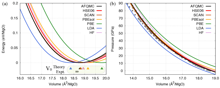
Figure 1: AFQMC, various DFT, and HF predictions of (a) the energy-volume relation and equilibrium volume $V_{0}$ (colored triangles) and (b) compression curve of B1 MgO at 300 K, benchmarked against experimental values (gray symbols) from Refs. 76, 77, 78. In (a), all energy curves are plotted relative to their respective minimum values.

To directly compare theoretical EOS with DAC experiments, corrections to the static-lattice results are needed to account for the differences due to lattice vibration and thermal contributions. We have added ion thermal contributions to the cold curve EOS via lattice vibration calculations under QHA, which is generally considered a good approximation for MgO under room temperature. The cold-curve EOS is re-evaluated by fitting the corrected 300-K data for each phase to the EOS models. The equilibrium volume and the pressure-volume results from theoretical calculations (AFQMC, DFT, and HF) are shown in Fig. 1 and compared to experimental results. It shows remarkable agreement between AFQMC and experimental results for both the equilibrium volume and compression curve. In contrast, the HF and DFT results scatter around the experimental values and vary significantly. Explicitly, DFT results exhibit a strong dependence on the choice of the xc functional, with HSE06, SCAN, and PBEsol performing better than PBE and LDA when compared with the experimental data.

Figure 2 compares the AFQMC cold curve of MgO at higher densities (near the B1-B2 transition) with those calculated using HF and DFT with various xc functionals. It shows HF, LDA and PBE demonstrate large deviations (approximately $\pm$0.5 to 1 eV/MgO in energy and 0 to 40 GPa in pressure, depending on the phase and the density) for the cold curves, while PBEsol, SCAN, and HSE06 show significantly improved agreements, in comparison to the AFQMC results. These findings are overall consistent with normal expectations based on Jacob’s ladder (precision relation: hybrid$>$meta-GGA$>$GGA/LDA$>$HF).

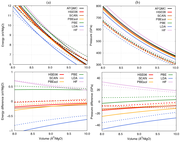
Figure 2: Comparison between AFQMC and various DFT or HF predictions of (a) internal energies and (b) pressures from static-lattice calculations of MgO around the B1-B2 transition. Top: direct comparisons; bottom: differences relative to AFQMC. Solid and dashed lines denote results for the B1 and B2 structures, respectively.

Figure 3 summarizes the B1-B2 phase transition pressures (red) and volume changes upon the phase transition (black) of MgO calculated using HF and DFT with various XC functionals in comparison to AFQMC. Due to the reconciliation of the EOS errors for the B1 and B2 phases in the calculation of the B1-B2 transition, the proximity of HF and DFT to AFQMC results no longer follows expectations of Jacob’s ladder. The AFQMC predicted transition pressure is lower and volumes upon transition are larger than all other methods. PBEsol prediction of the transition pressure is closer to AFQMC than HF or other DFT xc functionals, with a difference of 20 GPa.

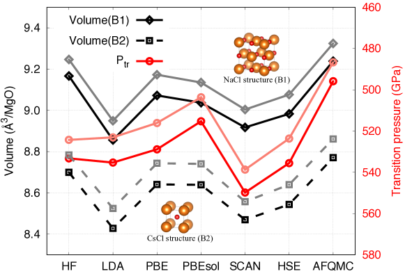
Figure 3: Comparison between AFQMC and various DFT or HF predictions of the volumes of the B1 and B2 phases upon transition and the transition pressure. Lighter colors denote 300-K results based on QHA; darker colors denote static-lattice results. The transition occurs at 429 to 562 GPa according to room-temperature experiments [28].

III.2 High-temperature EOS

High-temperature EOS of solid-state MgO is obtained from QMD and QHA calculations. The QHA results are based on a combination of phonon and cold-curve EOS, where the cold curves are obtained by static DFT calculations using four different xc functionals (LDA, PBE, PBEsol, and SCAN), while phonon calculations are performed by using the DFPT approach, PBEsol xc functional, Mg_sv_GW and O_h pseudopotentials, and including the Born effective charge. Tests show negligible differences in vibrational energies if the phonon calculations are done by using other xc functionals or ignoring the splitting between longitudinal and transverse optical modes (see Appendices C and D).

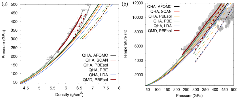
Figure 4: Comparison between QMD and QHA Hugoniots of MgO in (a) pressure-density and (b) temperature-pressure spaces. Different colors denote the different calculation methods. Solid and dashed curves represent results for B1 and B2 phases, respectively. Also included (in gray) are the experimental Hugoniot data from Marsh et al. (squares) [79], Vassiliou et al. (up triangles) [80], Fratanduono et al. (down triangles) [81], Root et al. (circles) [38], Svendsen and Ahrens et al. (diamonds) [82], McWilliams et al. (ovals) [11], and Bolis et al. (shaded areas, with a horizontal bar denoting the error in pressure and a cross denoting the condition interpreted as the melting point) [40], previous DFT-MD predictions based on the Armiento–Mattsson xc functional (line-crosses) [38], and a thermodynamic EOS model by de Koker and Stixrude (thick dashed lines) [31].

We first used the EOS to calculate the principal Hugoniot and compared them with experiments. Figure 4 shows comparisons of the Hugoniots in pressure–density and temperature–pressure spaces. Similar to previous QMD calculations that used the Armiento–Mattsson (AM05) xc functional [38], our present QMD results based on the PBEsol functional show excellent agreement with experimental Hugoniots in stability regimes of both B1 and B2 in the pressure-density relation, as well as for B1 in the temperature profile. In comparison, QHA results show consistency with experiments at low pressures but give increasingly higher density at high pressures along the Hugoniot, more so for the B2 than the B1 phase. The breakdown of QHA as shown in the pressure-density results can be attributed to the anharmonic vibration effect that is naturally included in QMD but missing in QHA and becomes more significant at higher temperatures. By comparing the thermal EOS along an isotherm, we found similar energies but higher pressures given by QMD than by QHA; according to the Rankine–Hugoniot equation, this must be reconciled by less shrinking in volume, which explains the Hugoniot density relations between QMD and QHA as shown in Fig. 4(a).

In the temperature-pressure space, QMD and QHA results of the Hugoniot are less distinct from each other than in the pressure-density space. QHA results based on LDA xc functional clearly lie below the range of the experimental data for the B1 phase, PBE significantly improves the agreement with experiments, while PBEsol and SCAN functionals and AFQMC data fall between LDA and PBE and near the lower bound of the experimental data. QMD predictions of the temperature are higher and improve over that by QHA using PBEsol. In addition, QMD predicts smaller differences between the Hugoniot of the B1 and B2 phases than QHA; AFQMC predictions of the B2 Hugoniot show good agreement with SCAN and LDA under QHA, following the trend of experimental Hugoniot after the turnover, while the QHA-PBEsol predictions are slightly higher. Our QMD results of the Hugoniot are overall consistent with previous calculations and align with experiments. More discussions will be given in the following and in Appendix G regarding the B1–B2 phase boundary and comparison between our prediction and the experiments.

The agreement with experiments in both the thermal (along the Hugoniot) and the cold-curve EOS (as shown in the previous Sec. III.1) validates PBEsol as an optimal choice for the xc functional for calculations of MgO at both the ground state and finite temperatures. In the following, we have added the QHA and QMD-derived (using the TDI approach) thermal free energies based on DFT-PBEsol calculations to various cold curves (by AFQMC and DFT-PBEsol/SCAN) to estimate the total free energies of MgO in both B1 and B2 phases . Based on these results, we charted the B1-B2 transition and calculate the volumes of the two phases upon transition. The results provide a preliminary reference for the B1-B2 phase boundary and its uncertainty based on state-of-art theoretical computations.

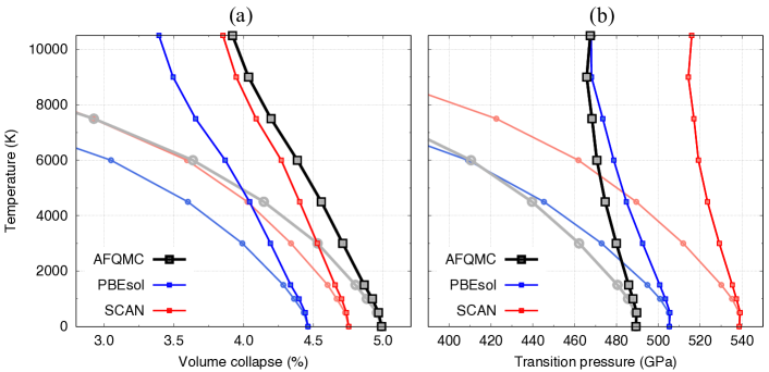
Figure 5: (a) Volume collapse and (b) pressures of the B1$\rightarrow$B2 transition at finite temperatures with the cold curve calculated using AFQMC and DFT with two optimal xc functionals (PBEsol and SCAN) and thermal effect (based on QMD and TDI) calculated within DFT using the PBEsol functional. Results based on QHA (including electron thermal but excluding anharmonic vibrational effects) are shown in lighter-colored curves (with circle symbols) for comparison.

Figure 5 shows the volume of MgO collapses by $\sim 4.75(\pm 0.25)\%$ at 0 K [from $\sim$9.2 ų/MgO for B1 to $\sim$8.7 ų/MgO for B2 (error associated with using different methods AFQMC, PBEsol, and SCAN: $\pm$0.1 ų/MgO)] and $3.7(\pm 0.2)\%$ at 10,500 K [from $\sim$9.8 ų/MgO for B1 to $\sim$9.4 ų/MgO for B2 (error: $\pm$0.2 ų/MgO)] for the B1$\rightarrow$B2 transition, and the transition pressure decreases from $\sim 515(\pm 25)$ GPa to $\sim 490(\pm 25)$ GPa as temperature increases from 0 to 10,500 K. We found the $V_{\text{tr}}-T$ curves are similar between the three sets of predictions based on AFQMC and DFT-PBEsol/SCAN cold curves, with the AFQMC predicted volumes and volume collapses larger (and transition pressures lower) than the DFT predictions. The $\mathrm{d}T/\mathrm{d}P$ Clapeyron slope of the B1-B2 phase boundary predicted by the AFQMC data set is similar to DFT-SCAN, both being steeper than that by DFT-PBEsol (see Table 4 that summarizes values of the Clapeyron slope).

Figure 5 also shows QHA predicts a much less steep boundary for the B1-B2 transition than QMD, reflecting the importance of anharmonic vibrational effects, similar to the report by previous studies [29, 37]. Our results clearly show the amounts of changes in volume and volume difference between the two phases of MgO upon transition, as well as the important role of electronic interactions (many-body in nature versus single-particle approximation under different xc functionals) in affecting the results. The much less negative value in Clapeyron slope ($dP_{\mathrm{tr}}/dT$) and slightly larger value in volume collapse of the B1–B2 transition predicted by QMD may cause less significant topography of discontinuity and lateral variations in deep-mantle mineralogy of super-Earths than previously expected based on the QHA results, changing expectations on the style of convection in these planets (see discussions in, e.g.,  [84]).

Moreover, by predicting a steeper B1–B2 boundary than latest theoretical studies [29, 37], our AFQMC (and PBEsol) results show excellent consistency with both experiments by McWilliams et al [11] and Bolis et al [40] (see Appendix G). We note that Bolis et al [40] interpreted the turnover in their experiments as the melting start of shocked MgO, largely based on comparisons with theoretical studies by then that underestimated $P_{\mathrm{tr}}$ along the Hugoniot. Our new results suggest that the turnovers in the experiments are associated with the B1–B2 transition. It is beyond the scope of this study, however, to decipher the nature of the subtle differences between experiments by Bolis et al. [40] and McWilliams et al. [11], as it requires accurate knowledges of the triple point, thermodynamic free energies of the liquid phase, as well as considerations of the kinetics of the transition to fully understand the observations.

We have performed additional tests and found the error in transition pressure (associated with the choices of different $T_{\text{ref}}$ and fitting methods in TDI) increases to $\sim$50 GPa at $T\approx 10^{4}$ K (see Appendix F, corresponding changes in the Clapeyron slope are tabulated in Table 4), while the errors due to other sources (EOS models, data error bars, and the data grid) are relatively small (e.g., the statistical error of the AFQMC and QMD energies only leads to a difference in $P_{\text{tr}}$ of 1.5 GPa at 6000 K).

IV Conclusions

This work exemplifies the first application of the AFQMC approach to benchmark the cold curve and phase transition in solid-state materials to very high pressures. Our AFQMC results reproduce the experimental cold curve (equilibrium volume and compressibility at room temperature) and provide a preliminary reference for the equations of state of MgO at up to 1 TPa. In comparison, DFT predictions vary by up to 7% to 15% for the equilibrium properties ($V_{0}$ and $B_{0}$) and B1-B2 transition ($P_{\text{tr}}$ and volume collapse upon the transition), depending on the xc functionals, and the largest differences are observed between the cold curves by PBE and LDA. The HSE06, SCAN, PBEsol functionals perform better than PBE, LDA, and HF in reproducing the $E(V)$ cold curves by AFQMC. The cold-curve differences for B1 offset those for B2, leading to the sensitivity of the predicted transition pressure and volume change to the choice of the xc functional.

Our Hugoniot results based on QMD calculations of the thermal EOS using PBEsol show excellent agreement with experiments for B1 and B2 in the pressure-density relation, as well as for B1 in the temperature-pressure profile. In comparison, QHA results of the pressure-density Hugoniot show consistency with experiments at low pressures but increasing discrepancy at high pressures, because larger anharmonic effects are expected at higher temperatures. The good performance of PBEsol in reproducing both the thermal (along the Hugoniot) and the cold-curve EOS of MgO has motivated us to further calculate the anharmonic free energies and add them to the cold curves by AFQMC and DFT-PBEsol or SCAN to calculate the total free energies and evaluate the B1-B2 transition at various temperatures. Our results show temperature lowers the transition pressure and expands the volumes upon the B1-B2 transition. Anharmonic vibration increases the transition pressure $P_{\text{tr}}$ and hinders the transition volumes $V_{\text{tr}}$ from expansion, relative to QHA. AFQMC predicts a steeper $\mathrm{d}T/\mathrm{d}P$ phase boundary and a larger volume collapse upon the B1$\rightarrow$B2 transition than DFT-PBEsol, similar to the effect of anharmonicity with respect to QHA.

In addition to providing a preliminary reference for the B1-B2 phase boundary and its uncertainty based on state-of-art theoretical computations, our results will be useful for building an accurate multiphase EOS table for MgO for planetary sciences and high energy density sciences applications, as well as for elucidating the mechanism of phase transformations (e.g., kinetics effects) in different experimental settings (e.g., compression rates). More work is desired to clarify the triple point and the melting curve at high temperatures and pressures to multi-TPa pressures. Looking ahead, finite-temperature AFQMC [85, 86], by better accounting of the electron thermal effects, and back-propagation for force and stress estimators in AFQMC [87] can offer additional yet more-accurate options to benchmark the EOS and phase transitions of solid-state materials at high temperatures and pressures.

Appendix A Finite-size and basis sets corrections to AFQMC energies

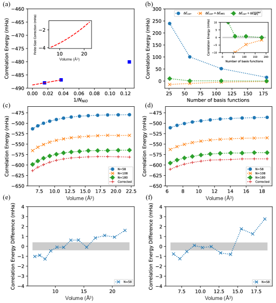
Figure 6: Examples of our AFQMC energies extrapolation: (a) finite-size correction [pVTZ ($N$=58)]; (b) AFQMC correlation energy measured with respect to the CBS limit; (c-d) uncorrected AFQMC correlation energies for various basis sets and, as a comparison, basis set corrected AFQMC energies with the pVTZ basis set; (e-f) the same red curves in panels (c-d) but now measured with respect to corrected pV5Z basis set results, showing the excellent agreement and efficiency of the basis set correction. Panels (a-b): 18.65 Å³/MgO; (b-f): $N_{\mathrm{NiO}}=8$; (a-c) and (e): B1; (d) and (f): B2. The inset of (a) shows the values of the finite-size corrections at different volumes. In (b), $\Delta E_{\mathrm{corr}}$ denotes uncorrected AFQMC energies, $\Delta E_{\mathrm{MP2}}$ represents the MP2 correction, and $\Delta E_{\mathrm{MP2}}^{\mathrm{scaled}}$ denotes the scaled MP2 correction. $N$ denotes the number of basis functions.

Our AFQMC calculations were performed for both phases of MgO at all volumes with various cell sizes and optimized basis sets. These include: (i) 2$\times$2$\times$2 $k$ points (8 MgO units) with pVDZ, pVTZ, pVQZ, and pV5Z; (ii) 3$\times$3$\times$3 $k$ points (27 MgO units) with pVTZ and pVQZ; and (iii) 4$\times$4$\times$4 $k$ points (64 MgO units) with pVTZ.

We have then followed three steps to extrapolate the AFQMC results to the thermodynamic and the complete basis set (CBS) limits:
1. Use all the pVTZ results to calculate finite size corrections for the 3$\times$3$\times$3 calculations;
2. Use all the 3$\times$3$\times$3 calculations to calculate the basis set corrections, combining AFQMC calculations with MP2 calculations and the “scaled” correction described in Ref. 27;
3. Use the 2$\times$2$\times$2 calculations to check reliability of the basis set corrections in step 2 and to ensure the basis set corrections were robust.

Our extrapolation procedure is demonstrated in Figure 6. The remarkable consistency between the pVTZ and pV5Z corrected values (to approximately 1–2 mHa/MgO from calculations with only 2$\times$2$\times$2 $k$ points) suggests our corrections are reliable and robust.

Appendix B EOS fit and transition pressure determination

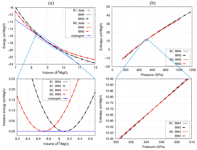
Figure 7: Determination of the transition pressure ($P_{\text{tr}}$) by using two different approaches: (a) common-tangent of the internal energy $E(V)$ curves and (b) intersect of the enthalpy $H(P)$ curves. In this example, the data are from 0-K DFT-PBEsol+QHA calculations; $P_{\text{tr}}$ determined using the two approaches are 504 and 505 GPa, respectively.

Figure 7 compares the two different ways of calculating the transition pressure: using internal energies $E(V)$ and their common tangent (left) or using enthalpies $H(P)$ and their crossover point . The two approaches are thermodynamically equivalent, as shown by the same transition pressure that has been determined (the 1-GPa difference is due to the numerical fitting of the data). The common-tangent approach is our option in this study because the internal energy (or Helmholtz free energy for $T\neq$ 0 K) is readily calculated while pressure is not except for the 0-K DFT cases.

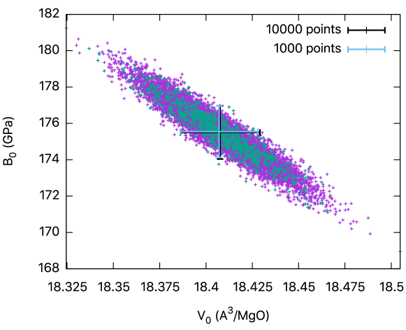
Figure 8: A Monte Carlo approach is used to determine the 1-$\sigma$ errors of the EOS fitting parameters. In this example, the AFQMC data and their standard errors (as shown in Table 1) are used and the third-order Birch–Murnaghan EOS model is considered. Two Monte Carlo runs with 1000 or 10000 randomly generates datasets give the same results for $V_{0}$, $B_{0}$, and their error bars.

The $E(V)$ data are fitted to EOS models to determine the equilibrium volume $V_{0}$ and bulk modulus $B_{0}$. Typical errors of these parameters can be calculated using the Monte Carlo approach and are shown in Fig. 8.

Table 3 summaries the equilibrium volume $V_{0}$ and bulk modulus $B_{0}$ by using different EOS models for the PBEsol data. We found the third-order Eulerian EOS (Birch–Murnaghan) works surprisingly well for MgO up to TPa pressures as long as data at high-enough pressures are included.

Table 3: Equilibrium volume ($V_{0}$), bulk modulus ($B_{0}$) and its pressure derivative ($B_{0}^{\prime}$), and volumes of transition ($V_{\text{tr}}$) of MgO in B1 and B2 phases, and the transition pressure ($P_{\text{tr}}$), determined in different fitting approaches for the $E(V)$ data from static DFT calculations using the PBEsol xc functional. Volumes are in units per Mg-O pair.

	$V_{0}^{\text{B1}}$ (Å3)	$B_{0}^{\text{B1}}$ (GPa)	$B_{0}^{\prime\text{B1}}$	$V_{0}^{\text{B2}}$ (Å3)	$B_{0}^{\text{B2}}$ (GPa)	$B_{0}^{\prime\text{B2}}$	$V_{\text{tr}}^{\text{B1}}$ (Å3)	$V_{\text{tr}}^{\text{B2}}$ (Å3)	$P_{\text{tr}}$ (GPa)
BM3	18.720	161.4	4.01	17.797	170.2	3.94	–	–	–
BM4	18.737	157.4	4.11	18.366	145.1	4.09	9.013	8.609	517.5
Vinet	18.786	137.7	4.91	20.552	68.5	5.56	9.012	8.583	522.7
BM3	18.721	160.4	4.02	18.266	151.3	3.99	–	–	–
BM4	18.737	157.3	4.11	18.289	147.6	4.09	9.014	8.610	517.4
Vinet	18.791	141.1	4.81	18.364	129.2	4.86	9.037	8.639	515.3
spline	–	–	–	–	–	–	9.001	8.605	518.5

Appendix C Effect of LO-TO splitting

It is well known that the frequencies of the optical modes parallel and perpendicular to the electric field split (“LO-TO splitting”) in ionic materials such as MgO. [89] This mode splitting is missed in regular phonon calculations but can be correctly captured when Born effective charges, piezoelectric constants, and the ionic contribution to the dielectric tensor are considered (by switching on LEPSILON in VASP). The effects on the phonon dispersion relations of B1- and B2-MgO are shown in Fig. 9.

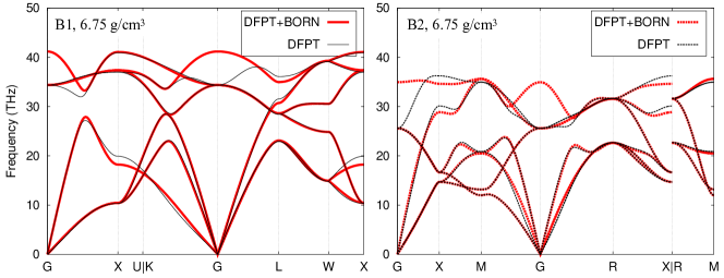
Figure 9: Phonon band structures of MgO from DFPT vs DFPT+Born calculations of B1 vs B2 MgO at 6.75 g/cm³.

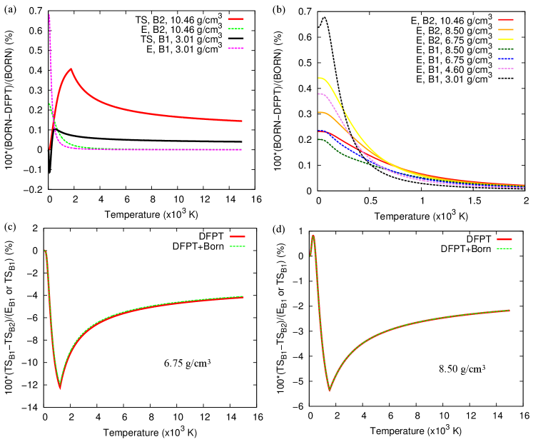
Figure 10: The effects of including LO-TO splitting (BORN) in phonon calculations on the thermodynamic properties of B1 and B2 phases of MgO at various densities. (a) Entropy and internal energy and (b) internal energy changes due to excluding LO-TO splitting; (c) and (d) entropy differences between B1 and B2 at two densities near the phase transition with and without LO-TO splitting. The differences in (c) and (d) are relative to $E$ or $TS$, whichever is larger.

Figure 10 compares the resultant differences in vibrational energy and entropy of MgO in different phases and at different densities. The results show that LO-TO splitting only makes a small difference ($<$0.7%) at $T<500$ K and then quickly drops to zero at higher T; the effect on the differences between B1 and B2 is also small and negligible.

Appendix D Effects of xc functional on phonon results

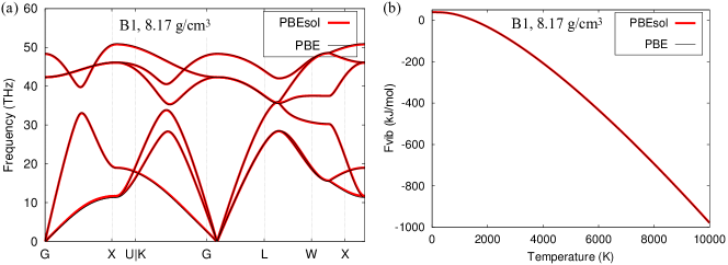
Figure 11: (a) Phonon band structures and (b) vibrational free energies of MgO from PBEsol vs PBE calculations.

Figure 11 shows that different xc functionals produce the same phonon band structure and vibrational free energies within QHA.

Appendix E Convergence test

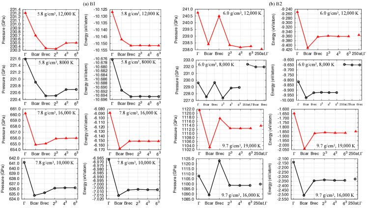
Figure 12: Finite size effects on pressures and internal energies of (a) B1 and (b) B2 structures of MgO at different densities and electronic temperatures. All calculations are based on DFT-PBEsol and use 64-atom cells for B1 and 54-atom cells for B2, unless otherwise specified. “Bcar” and “Brec” denotes using the special $k$ point of $(1/4,1/4,1/4)$ in cartesian (wrong “Baldereschi point” for cubic cell) and reciprocal (correct “Baldereschi point” for cubic cell) coordinates, respectively.

Figure 12 shows large cell sizes in combination with proper/fine $k$-point meshes are needed to ensure convergence of the EOS. For example, a 250-atom cell with a single $k$ point is not enough for B2 at 6.0 g/cm³. In our QMD simulations, we use a 64-atom cell with the “Brec” special $k$ point and a 54-atom cell with a $\Gamma$-centered 2$\times$2$\times$2 $k$ mesh, respectively, for the B1 and B2 calculations.

Our additional tests for the phonon calculations show that 8- and 16-atom cells, respectively, are needed for B1 and B2 to obtain converged $F_{\text{vib}}(T)$ results rather than using the primitive 2-atom cells. In this study, we choose 54-atom cells (with a 4$\times$4$\times$4 $k$ mesh) for both B1 and B2 phonon calculations for better accuracy.

Appendix F Calculation of anharmonic energies and comparison between different terms

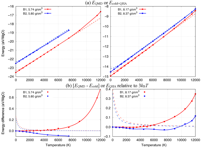
Figure 13: (a) Internal energies along selected isochores of MgO based on QMD (darker solid curves) or QHA (lighter dashed curves) calculations. (b) Differences of the ion thermal term of the internal energy (QMD: solid curves and symbols; QHA: dashed curves) from a classical crystal that assumes 3$k_{\text{B}}$/atom for the heat capacity (the Dulong–Petit law). The structures and densities are represented by different colors and symbols as denoted in the legend. The solid curves in (b) are polynomial fits to the data. In both panels, $E_{\text{cold}}$ is taken as the value of $E_{\text{QMD}}$ at 0 K.

Figure 13 shows the finite-temperature internal energies of MgO estimated from cold calculations under QHA ($E_{\text{cold+QHA}}$) in comparison with values from direct QMD simulations ($E_{\text{QMD}}$). Overall, $E_{\text{cold+QHA}}$ and $E_{\text{QMD}}$ are similar to each other, with noticeable differences near zero K, because of the nuclear quantum effects, or at high temperatures, due to increased anharmonic vibration and electron excitation effects. The differences are more evident when the ion thermal energies ($E-E_{\text{cold}}$) are plotted with respect to the classical crystal value of $3k_{B}T$. The mismatch between QMD and QHA near zero K and the proximity of $E_{\text{QHA}}$ to $3k_{B}T$ at high temperatures have motivated us to define $E_{\text{anharm}}=E_{\text{QMD}}-E_{\text{cold+QHA}}\approx E_{\text{QMD}}-E_{\text{cold}}-3k_{B}T$ in the TDI Eq. 6 to calculate the anharmonic free energy $F_{\text{anharm}}$. Under this approximation, the total free energy of the system $F(V,T)=E_{\mathrm{cold}}(V)+F_{\mathrm{i},\mathrm{QHA}}(V,T)+F_{\mathrm{i}-\mathrm{th},\mathrm{anharm}}(V,T)+F_{\mathrm{e}-\mathrm{{\color[rgb]{0,0,0}th}}}(V,T)\approx E_{\mathrm{cold}}(V)+F_{\mathrm{ind.ph.}}^{\mathrm{quantum.}}(V,T)+F_{\mathrm{int.ph.}}^{\mathrm{class.}}(V,T)+F_{\mathrm{e}-\mathrm{{\color[rgb]{0,0,0}th}}}(V,T)$ where the subindices “ind.” and “int.” denote independent and interacting, “ph.” denotes phonon, “class.” and “quantum.” represents the nature of the ions as being classical and quantum, respectively, and “e-th” denotes the electron thermal term. The only difference from an entirely accurate (“quantum”) description lies in the approximation in the anharmonic term by using classical ions (as in QMD simulations and the classical-crystal reference for TDI), whose effect, we believe, is negligible for the purpose of this paper. We have performed extensive tests and found $E_{\text{anharm}}(V,T)$ can be isochorically fitted well using sixth- and eighth-order polynomials for the B1 and B2 phases, respectively. We also note that the different choices of $T_{\text{ref}}$ or fitting $E_{\text{QMD}}$ by using cubic splines can affect the value of $F_{\text{anharm}}$ (see Fig. 14), while lower-order polynomials or exponential fits [2, 90], although they were found to work for certain materials at ambient densities or relatively low temperatures, break down for MgO at high densities and temperatures.

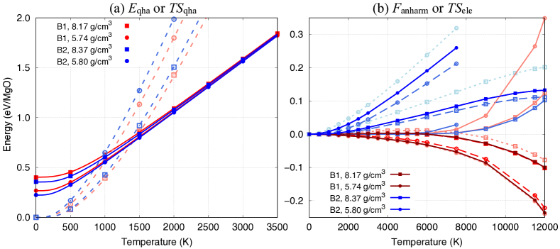
Figure 14: Comparison between different thermodynamic energy terms of MgO, including (a) internal energy (solid curves) and vibration entropy (dashed curves) terms under QHA calculations, and (b) anharmonic free energy (dark solid and light dashed curves) and electronic entropy (light solid curves) terms from TDI and QMD calculations. The anharmonic free energies shown in (b) are calculated using TDI with different methods: polynomial fit of anharmonic internal energy ($E_{\text{anharm}}=E_{\text{QMD}}-E_{\text{cold}}-3k_{B}T$) with $C_{V}(T_{\text{ref}})$=10%$\times 3k_{\text{B}}$/atom (dark solid, corresponding $T_{\mathrm{ref}}$=100–200 K) or 90%$\times 3k_{\text{B}}$/atom (light long dashed, corresponding $T_{\mathrm{ref}}$=800–1550 K) or cubic spline fit of the internal energy ($E_{\text{QMD}}$) with $C_{V}(T_{\text{ref}})$=50%$\times 3k_{\text{B}}$/atom (light short dashed, corresponding $T_{\mathrm{ref}}$=250–550 K).

In practice, QMD is less efficient and inappropriate for simulating near-zero temperatures. Therefore we have to choose a finite value for $T_{\text{ref}}$ in TDI and assume QHA is valid for any temperature below $T_{\text{ref}}$. This would technically limit the accuracy of the anharmonic free energies, as shown in Fig. 14(b) by the different values of $F_{\text{anharm}}$ when choosing different $T_{\text{ref}}$ and fitting approaches. Figure 14 also shows that the contributions by electron thermal excitation become increasingly significant when the temperature exceeds 8000 K, more at lower densities. The anharmonic vibration and electron thermal terms are relatively small in comparison to the lattice vibration as accounted under QHA. However, because of the similarities between energies of the B1 and B2 phases, the effects of anharmonic vibration can significantly affect the B1-B2 transition boundary, as shown in Fig. 5.

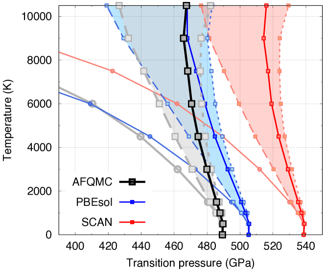
Figure 15: B1-B2 phase boundary calculated using QHA (light solid line-circles) in comparison to those including the anharmonic effect calculated with three different methods in TDI: polynomial fit of $E_{\text{anharm}}$ with $C_{V}(T_{\text{ref}})$=10%$\times 3k_{\text{B}}$/atom (dark solid line-squares, corresponding $T_{\mathrm{ref}}$=100–200 K) or 90%$\times 3k_{\text{B}}$/atom (light long dashed line-squares, corresponding $T_{\mathrm{ref}}$=800–1550 K) or cubic spline fit of the internal energy ($E_{\text{QMD}}$) with $C_{V}(T_{\text{ref}})$=50%$\times 3k_{\text{B}}$/atom (light short dashed line-squares, corresponding $T_{\mathrm{ref}}$=250–550 K). The maximum range of difference defined by the three methods are represented by the shaded area. Black, blue, and red colors denote the calculations that use different cold curves.

Figure 15 summarizes the B1-B2 transition pressure based on free energies calculated using different approaches. Despite the distinctions between predictions by AFQMC and DFT-PBEsol or SCAN at zero K, all methods give similar trends of decreasing $P_{\text{tr}}$ (by $\sim$20 to 40 GPa at 9000 K, relative to the corresponding values at 0 K) and enlarging uncertainty (by $\sim$40 to 50 GPa at 9000 K) as temperature increases. The relations in $P_{\text{tr}}$ between the different approaches AFQMC, DFT-PBEsol, and DFT-SCAN at high temperatures remain similar to those under QHA, whereas the anharmonic effects clearly steepen the $\mathrm{d}T/\mathrm{d}P$ slope and push $P_{\text{tr}}$ to higher values than QHA predictions. With polynomial fits of $E_{\text{anharm}}$, the differences between the phase boundaries based on QHA and anharmonic calculations are smaller if the values of $T_{\text{ref}}$ are higher (light long dashed line-squares); in comparison, cubic spline fits of $E_{\text{QMD}}$ using the same $T_{\text{ref}}$ tend to produce larger differences than the polynomial fits of $E_{\text{anharm}}$ (light short dashed line-squares). We have quantified the phase-boundary differences by calculating the Clapeyron slope. The results are summarized in Table 4.

Table 4: Clapeyron slope $dP_{\mathrm{tr}}/dT$ (in units of MPa/K) of the MgO B1–B2 phase transition estimated by linear regression of the data calculated using different approaches as shown in Fig. 15. The calculations for QHA use 1500–4500 K data, while other cases use 1500–6000 K data, for better linearity and relevance to the super-Earths’ interior conditions. Numbers in boldface correspond to the solid line squares in Figs. 5(b) and 15. We note that the values of the slope calculated here are much smaller than previous estimations based on experiments ($-390\pm 300$ MPa/K) [11], which were associated with significant uncertainties, and also lower than predictions by an interatomic model of the B1-B2 transition ($\sim-40$ MPa/K if taking volume collapse of 3% and entropy increase of 7 J/K/mol) [91, 92], suggesting the B1-B2 entropy difference and the thermodynamic properties of MgO are sensitive to pressure and different from the underlying assumptions of the model.

	QHA	$C_{V}(T_{\text{ref}})$=10%$\times 3k_{\text{B}}$/atom	$C_{V}(T_{\text{ref}})$=90%$\times 3k_{\text{B}}$/atom	$C_{V}(T_{\text{ref}})$=50%$\times 3k_{\text{B}}$/atom
AFQMC	-13.6 $\pm$ 0.8	-3.4 $\pm$ 0.2	-6.8 $\pm$ 0.1	-2.3 $\pm$ 0.3
SCAN	-13.5 $\pm$ 0.8	-3.6 $\pm$ 0.2	-7.1 $\pm$ 0.1	-2.7 $\pm$ 0.3
PBEsol	-16.5 $\pm$ 1.1	-4.9 $\pm$ 0.2	-8.9 $\pm$ 0.1	-3.8 $\pm$ 0.3

Furthermore, we have tested by employing two different versions of the TDI/temperature-integration approach to cross-check our above results, including (1) a more direct approach [93]:

$$\frac{F(V,T)}{T}-\frac{F(V,T_{\mathrm{ref}})}{T_{\mathrm{ref}}}=\int_{1/T_{\mathrm{ref}}}^{1/T}E(V,\mathcal{T})\mathrm{d}\frac{1}{\mathcal{T}}$$ (7)

and (2) an indirect approach [by taking the difference of Eq. 7 with respect to a reference system (e.g., the system under QHA) that also satisfies Eq. 7]:

$$F(V,T)-F_{\mathrm{ref}}(V,T)=T\int_{1/T_{\mathrm{ref}}}^{1/T}[E(V,\mathcal{T})-E_{\mathrm{ref}}(V,\mathcal{T})]\mathrm{d}\frac{1}{\mathcal{T}}.$$ (8)

These tests were performed at $T=$3000, 6000, and 9000 K, with $T_{\mathrm{ref}}$ fixed to 500 K for simplicity. In approach (1), the free energy at $T_{\mathrm{ref}}$ is approximated by the corresponding values under QHA; in approach (2), the QHA system is taken as the reference, which defines $F_{\mathrm{ref}}$ and $E_{\mathrm{ref}}$. In both approaches, an additional term $E_{\mathrm{QC}}(V,\mathcal{T})=E_{\mathrm{QHA}}(V,\mathcal{T})-3k_{\mathrm{B}}\mathcal{T}$ has been introduced as quantum correction of the internal energy from QMD, similar to that in Ref. 94. We note that the quantum correction is crucial to obtain accurate free energies within the temperature integration approach, which starts from a cold reference state where the important nuclear quantum effects are included by QHA but missed in QMD. We also note that, with the quantum correction and with $E_{\mathrm{cold}}$ deducted from all energy terms, Eq. 8 is equivalent to our method introduced in detail above and in Sec. II.2 (Eq. 6).

Based on our PBEsol data (cold curve, QHA, and QMD), the free energies calculated using these two approaches are similar, both producing similar B1–B2 transition pressures: 486 GPa at 3000 K, 462 GPa at 6000 K, and 439 GPa at 9000 K. The excellent consistency of the results from the tests with those shown in Fig. 15 (blue shaded area) reconfirms the methodology and findings of this study.

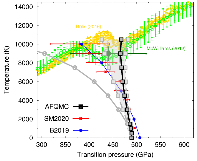
Figure 16: The B1–B2 phase boundary of MgO calculated in this study (same as the black/grey AFQMC results shown in Fig. 15) in comparison to shock experiments by McWilliams et al. [11] (green symbols) and Bolis et al. [40, 95] (yellow symbols) and recent theoretical calculations by Bouchet et al. [29] (temperature-dependent effective potential approach, LDA xc functional, data represented by blue line-circles) and Soubiran and Militzer [37] (TDI based on MD using effective potentials tuned between harmonic oscillators and Kohn–Sham DFT, PBE xc functional, data shown with red crosses). The dark-green circle denotes the condition attributed to the B1–B2 transition by McWilliams et al. [11].

Appendix G Comparison with experiments

Figure 16 compares our AFQMC results of the B1–B2 transition to shock experiments [11, 40] and recent theoretical calculations [29, 37]. The previous calculations were based on LDA/PBE, and their predicted $P_{\mathrm{tr}}$ at 0 K is larger than our AFQMC prediction, consistent with our findings shown in Fig. 3. The differences get smaller at higher temperatures until approximately 8000 K, above which the previous calculations show a lower $P_{\mathrm{tr}}$ and thus a less steep Clapeyron slope than ours. Our estimation of the B1–B2 phase boundary, with uncertainty, agrees with the wiggled regions in both experiments by McWilliams et al. [11] and Bolis et al. [40]. This suggests the turnovers in both experiments can be associated with the B1–B2 transition. To fully unveil the origins of the subtle differences between the measurements, however, still requires improved experimental diagnostics and theoretical constraints on the structure, kinetics, and thermodynamic conditions of the samples under shock compression.

References

- Murakami et al. [2004] M. Murakami, K. Hirose, K. Kawamura, N. Sata, and Y. Ohishi, Post-perovskite phase transition in MgSiO3., Science (New York, N.Y.) 304, 855 (2004).
- Oganov and Ono [2004] A. R. Oganov and S. Ono, Theoretical and experimental evidence for a post-perovskite phase of MgSiO3 in Earth’s D” layer, Nature 430, 445 (2004).
- Tsuchiya et al. [2004] T. Tsuchiya, J. Tsuchiya, K. Umemoto, and R. M. Wentzcovitch, Phase transition in MgSiO3 perovskite in the earth’s lower mantle, Earth Planet. Sci. Lett. 224, 241 (2004).
- Zhang et al. [2013] S. Zhang, H. F. Wilson, K. P. Driver, and B. Militzer, H 4 O and other hydrogen-oxygen compounds at giant-planet core pressures, Phys. Rev. B 87, 024112 1 (2013).
- Peng et al. [2020] F. Peng, X. Song, C. Liu, Q. Li, M. Miao, C. Chen, and Y. Ma, Xenon iron oxides predicted as potential Xe hosts in Earth’s lower mantle, Nature Commun. 11, 5227 (2020).
- Celliers et al. [2018] P. M. Celliers, M. Millot, S. Brygoo, R. S. McWilliams, D. E. Fratanduono, J. R. Rygg, A. F. Goncharov, P. Loubeyre, J. H. Eggert, J. L. Peterson, N. B. Meezan, S. Le Pape, G. W. Collins, R. Jeanloz, and R. J. Hemley, Insulator-metal transition in dense fluid deuterium., Science (New York, N.Y.) 361, 677 (2018).
- Rillo et al. [2019] G. Rillo, M. A. Morales, D. M. Ceperley, and C. Pierleoni, Optical properties of high-pressure fluid hydrogen across molecular dissociation, Proc. Natl. Acad. Sci. USA 116, 9770 (2019).
- Zurek and Bi [2019] E. Zurek and T. Bi, High-temperature superconductivity in alkaline and rare earth polyhydrides at high pressure: A theoretical perspective, J. Chem. Phys. 150, 50901 (2019).
- Dubrovinskaia et al. [2016] N. Dubrovinskaia, L. Dubrovinsky, N. A. Solopova, A. Abakumov, S. Turner, M. Hanfland, E. Bykova, M. Bykov, C. Prescher, V. B. Prakapenka, S. Petitgirard, I. Chuvashova, B. Gasharova, Y.-L. Mathis, P. Ershov, I. Snigireva, and A. Snigirev, Terapascal static pressure generation with ultrahigh yield strength nanodiamond, Sci. Adv. 2, e1600341 (2016).
- Jenei et al. [2018] Z. Jenei, E. F. O’Bannon, S. T. Weir, H. Cynn, M. J. Lipp, and W. J. Evans, Single crystal toroidal diamond anvils for high pressure experiments beyond 5 megabar, Nature Commun. 9, 3563 (2018).
- McWilliams et al. [2012] R. S. McWilliams, D. K. Spaulding, J. H. Eggert, P. M. Celliers, D. G. Hicks, R. F. Smith, G. W. Collins, and R. Jeanloz, Phase transformations and metallization of magnesium oxide at high pressure and temperature, Science 338, 1330 (2012).
- Coppari et al. [2013] F. Coppari, R. F. Smith, J. H. Eggert, J. Wang, J. R. Rygg, a. Lazicki, J. a. Hawreliak, G. W. Collins, and T. S. Duffy, Experimental evidence for a phase transition in magnesium oxide at exoplanet pressures, Nature Geosci. 6, 926 (2013).
- Millot et al. [2015] M. Millot, N. Dubrovinskaia, A. Černok, S. Blaha, L. Dubrovinsky, D. G. Braun, P. M. Celliers, G. W. Collins, J. H. Eggert, and R. Jeanloz, Shock compression of stishovite and melting of silica at planetary interior conditions, Science 347, 418 (2015).
- Kohn and Sham [1965] W. Kohn and L. J. Sham, Self-consistent equations including exchange and correlation effects, Phys. Rev. 140, A1133 (1965).
- Zhang et al. [2018] S. Zhang, F. D. Malone, and M. A. Morales, Auxiliary-field quantum Monte Carlo calculations of the structural properties of nickel oxide, J. Chem. Phys. 149, 164102 (2018).
- Driver et al. [2010] K. P. Driver, R. E. Cohen, Z. Wu, B. Militzer, P. L. Ríos, M. D. Towler, R. J. Needs, and J. W. Wilkins, Quantum Monte Carlo computations of phase stability, equations of state, and elasticity of high-pressure silica., Proc. Natl. Acad. Sci. USA 107, 9519 (2010).
- Trail et al. [2017] J. Trail, B. Monserrat, P. López Ríos, R. Maezono, and R. J. Needs, Quantum monte carlo study of the energetics of the rutile, anatase, brookite, and columbite polymorphs, Phys. Rev. B 95, 121108 (2017).
- Malone et al. [2019] F. D. Malone, S. Zhang, and M. A. Morales, Overcoming the Memory Bottleneck in Auxiliary Field Quantum Monte Carlo Simulations with Interpolative Separable Density Fitting, J. Chem. Theory Comput. 15, 256 (2019).
- Malone et al. [2020] F. D. Malone, A. Benali, M. A. Morales, M. Caffarel, P. R. C. Kent, and L. Shulenburger, Systematic comparison and cross-validation of fixed-node diffusion monte carlo and phaseless auxiliary-field quantum monte carlo in solids, Phys. Rev. B 102, 161104 (2020).
- LeBlanc et al. [2015] J. P. F. LeBlanc, A. E. Antipov, F. Becca, I. W. Bulik, G. K.-L. Chan, C.-M. Chung, Y. Deng, M. Ferrero, T. M. Henderson, C. A. Jiménez-Hoyos, E. Kozik, X.-W. Liu, A. J. Millis, N. V. Prokof’ev, M. Qin, G. E. Scuseria, H. Shi, B. V. Svistunov, L. F. Tocchio, I. S. Tupitsyn, S. R. White, S. Zhang, B.-X. Zheng, Z. Zhu, and E. Gull (Simons Collaboration on the Many-Electron Problem), Solutions of the two-dimensional hubbard model: Benchmarks and results from a wide range of numerical algorithms, Phys. Rev. X 5, 041041 (2015).
- Motta et al. [2017] M. Motta, D. M. Ceperley, G. K.-L. Chan, J. A. Gomez, E. Gull, S. Guo, C. A. Jiménez-Hoyos, T. N. Lan, J. Li, F. Ma, A. J. Millis, N. V. Prokof’ev, U. Ray, G. E. Scuseria, S. Sorella, E. M. Stoudenmire, Q. Sun, I. S. Tupitsyn, S. R. White, D. Zgid, and S. Zhang (Simons Collaboration on the Many-Electron Problem), Towards the solution of the many-electron problem in real materials: Equation of state of the hydrogen chain with state-of-the-art many-body methods, Phys. Rev. X 7, 031059 (2017).
- Zheng et al. [2017] B.-X. Zheng, C.-M. Chung, P. Corboz, G. Ehlers, M.-P. Qin, R. M. Noack, H. Shi, S. R. White, S. Zhang, and G. K.-L. Chan, Stripe order in the underdoped region of the two-dimensional hubbard model, Science 358, 1155 (2017).
- Lee et al. [2020] J. Lee, F. D. Malone, and D. R. Reichman, The performance of phaseless auxiliary-field quantum Monte Carlo on the ground state electronic energy of benzene, J. Chem. Phys. 153, 126101 (2020).
- Shi and Zhang [2021] H. Shi and S. Zhang, Some recent developments in auxiliary-field quantum Monte Carlo for real materials, J. Chem. Phys. 154, 24107 (2021).
- Zhang and Krakauer [2003] S. Zhang and H. Krakauer, Quantum monte carlo method using phase-free random walks with slater determinants, Phys. Rev. Lett. 90, 136401 (2003).
- Motta and Zhang [2018] M. Motta and S. Zhang, Ab initio computations of molecular systems by the auxiliary-field quantum monte carlo method, WIREs Comput. Mol. Sci. 8, e1364 (2018).
- Morales and Malone [2020] M. A. Morales and F. D. Malone, Accelerating the convergence of auxiliary-field quantum Monte Carlo in solids with optimized Gaussian basis sets, J. Chem. Phys. 153, 194111 (2020).
- Dubrovinskaia et al. [2019a] N. Dubrovinskaia, S. Petitgirard, S. Chariton, R. Tucoulou, J. Garrevoet, K. Glazyrin, H.-P. Liermann, V. B. Prakapenka, and L. Dubrovinsky, B1-B2 phase transition in MgO at ultra-high static pressure, arXiv preprint arXiv:1904.00476 (2019a).
- Bouchet et al. [2019] J. Bouchet, F. Bottin, V. Recoules, F. Remus, G. Morard, R. M. Bolis, and A. Benuzzi-Mounaix, Ab initio calculations of the B1-B2 phase transition in MgO, Phys. Rev. B 99, 094113 (2019).
- Alfè [2005] D. Alfè, Melting curve of mgo from first-principles simulations, Phys. Rev. Lett. 94, 235701 (2005).
- De Koker and Stixrude [2009] N. De Koker and L. Stixrude, Self-consistent thermodynamic description of silicate liquids, with application to shock melting of MgO periclase and MgSiO3 perovskite, Geophys. J. Int. 178, 162 (2009).
- Belonoshko et al. [2010] A. B. Belonoshko, S. Arapan, R. Martonak, and A. Rosengren, Mgo phase diagram from first principles in a wide pressure-temperature range, Phys. Rev. B 81, 054110 (2010).
- Boates and Bonev [2013] B. Boates and S. a. Bonev, Demixing Instability in Dense Molten MgSiO3 and the Phase Diagram of MgO, Phys/ Rev. Lett. 110, 135504 (2013).
- Cebulla and Redmer [2014] D. Cebulla and R. Redmer, Ab initio simulations of MgO under extreme conditions, Physical Review B 89, 134107 (2014).
- Taniuchi and Tsuchiya [2018] T. Taniuchi and T. Tsuchiya, The melting points of MgO up to 4 TPa predicted based on ab initio thermodynamic integration molecular dynamics, J. Phys.: Condens. Matter 30, 114003 (2018).
- Musella et al. [2019] R. Musella, S. Mazevet, and F. Guyot, Physical properties of MgO at deep planetary conditions, Phys. Rev. B 99, 064110 (2019).
- Soubiran and Militzer [2020] F. Soubiran and B. Militzer, Anharmonicity and Phase Diagram of Magnesium Oxide in the Megabar Regime, Phys. Rev. Lett. 125, 175701 (2020).
- Root et al. [2015] S. Root, L. Shulenburger, R. W. Lemke, D. H. Dolan, T. R. Mattsson, and M. P. Desjarlais, Shock Response and Phase Transitions of MgO at Planetary Impact Conditions, Phys. Rev. Lett. 115, 1 (2015).
- Miyanishi et al. [2015] K. Miyanishi, Y. Tange, N. Ozaki, T. Kimura, T. Sano, Y. Sakawa, T. Tsuchiya, and R. Kodama, Laser-shock compression of magnesium oxide in the warm-dense-matter regime, Phys. Rev. E 92, 23103 (2015).
- Bolis et al. [2016] R. M. Bolis, G. Morard, T. Vinci, A. Ravasio, E. Bambrink, M. Guarguaglini, M. Koenig, R. Musella, F. Remus, J. Bouchet, N. Ozaki, K. Miyanishi, T. Sekine, Y. Sakawa, T. Sano, R. Kodama, F. Guyot, and A. Benuzzi-Mounaix, Decaying shock studies of phase transitions in MgO-SiO2 systems: Implications for the super-Earths’ interiors, Geophys. Res. Lett. 43, 9475 (2016).
- Hansen et al. [2021] L. E. Hansen, D. E. Fratanduono, S. Zhang, D. G. Hicks, T. Suer, Z. K. Sprowal, M. F. Huff, X. Gong, B. J. Henderson, D. N. Polsin, M. Zaghoo, S. X. Hu, G. W. Collins, and J. R. Rygg, Melting of magnesium oxide up to two terapascals using double-shock compression, Phy. Rev. B 104, 014106 (2021).
- Hubbard [1959] J. Hubbard, Calculation of partition functions, Phys. Rev. Lett. 3, 77 (1959).
- Ceperley and Alder [1980] D. M. Ceperley and B. J. Alder, Ground state of the electron gas by a stochastic method, Phys. Rev. Lett. 45, 566 (1980).
- Zhang et al. [1997] S. Zhang, J. Carlson, and J. E. Gubernatis, Constrained path monte carlo method for fermion ground states, Phys. Rev. B 55, 7464 (1997).
- Shee et al. [2019] J. Shee, B. Rudshteyn, E. J. Arthur, S. Zhang, D. R. Reichman, and R. A. Friesner, On achieving high accuracy in quantum chemical calculations of 3d transition metal-containing systems: A comparison of auxiliary-field quantum monte carlo with coupled cluster, density functional theory, and experiment for diatomic molecules, J. Chem. Theory Comput. 15, 2346 (2019).
- Purwanto et al. [2009] W. Purwanto, S. Zhang, and H. Krakauer, Excited state calculations using phaseless auxiliary-field quantum monte carlo: Potential energy curves of low-lying c2 singlet states, J. Chem. Phys. 130, 094107 (2009).
- Borda et al. [2018] E. J. L. Borda, J. A. Gomez, and M. A. Morales, Non-orthogonal multi-slater determinant expansions in auxiliary field quantum monte carlo, arXiv preprint arXiv:1801.10307 (2018).
- Mahajan and Sharma [2021] A. Mahajan and S. Sharma, Taming the sign problem in auxiliary-field quantum monte carlo using accurate wave functions, J. Chem. Theory Comput. 17, 4786 (2021).
- Qin et al. [2016] M. Qin, H. Shi, and S. Zhang, Benchmark study of the two-dimensional hubbard model with auxiliary-field quantum monte carlo method, Phys. Rev. B 94, 085103 (2016).
- Chang and Morales [2017] C.-C. Chang and M. A. Morales, Multi-determinant generalized hartree-fock wave functions in monte carlo calculations, arXiv preprint arXiv:1711.02154 (2017).
- Giannozzi et al. [2009] P. Giannozzi, S. Baroni, N. Bonini, M. Calandra, R. Car, C. Cavazzoni, D. Ceresoli, G. L. Chiarotti, M. Cococcioni, I. Dabo, A. D. Corso, S. de Gironcoli, S. Fabris, G. Fratesi, R. Gebauer, U. Gerstmann, C. Gougoussis, A. Kokalj, M. Lazzeri, L. Martin-Samos, N. Marzari, F. Mauri, R. Mazzarello, S. Paolini, A. Pasquarello, L. Paulatto, C. Sbraccia, S. Scandolo, G. Sclauzero, A. P. Seitsonen, A. Smogunov, P. Umari, and R. M. Wentzcovitch, Quantum espresso: a modular and open-source software project for quantum simulations of materials, J. Phys.: Condens. Matter 21, 395502 (2009).
- Giannozzi et al. [2017] P. Giannozzi, O. Andreussi, T. Brumme, O. Bunau, M. Buongiorno Nardelli, M. Calandra, R. Car, C. Cavazzoni, D. Ceresoli, M. Cococcioni, N. Colonna, I. Carnimeo, A. Dal Corso, S. de Gironcoli, P. Delugas, R. A. DiStasio, Jr., A. Ferretti, A. Floris, G. Fratesi, G. Fugallo, R. Gebauer, U. Gerstmann, F. Giustino, T. Gorni, J. Jia, M. Kawamura, H.-Y. Ko, A. Kokalj, E. Küçükbenli, M. Lazzeri, M. Marsili, N. Marzari, F. Mauri, N. L. Nguyen, H.-V. Nguyen, A. Otero-de-la-Roza, L. Paulatto, S. Poncé, D. Rocca, R. Sabatini, B. Santra, M. Schlipf, A. P. Seitsonen, A. Smogunov, I. Timrov, T. Thonhauser, P. Umari, N. Vast, X. Wu, and S. Baroni, Advanced capabilities for materials modelling with Quantum ESPRESSO, J. Phys.: Condens. Matter 29, 465901 (2017).
- F. and Jan [1977] B. N. H. F. and L. Jan, Simplifications in the generation and transformation of two‐electron integrals in molecular calculations, Int. J. Quantum Chem. 12, 683 (1977).
- Koch et al. [2003] H. Koch, A. S. de Merás, and T. B. Pedersen, Reduced scaling in electronic structure calculations using cholesky decompositions, J. Chem. Phys. 118, 9481 (2003).
- Francesco et al. [2009] A. Francesco, D. V. Luca, F. Nicolas, G. Giovanni, M. Per‐åke, N. Pavel, P. T. Bondo, P. Michal, R. Markus, R. B. O., S. Luis, U. Miroslav, V. Valera, and L. Roland, Molcas 7: The next generation, J. Comput. Chem. 31, 224 (2009).
- Purwanto et al. [2011] W. Purwanto, H. Krakauer, Y. Virgus, and S. Zhang, Assessing weak hydrogen binding on ca+ centers: An accurate many-body study with large basis sets, J. Chem. Phys. 135, 164105 (2011).
- Hamann [2013] D. R. Hamann, Optimized norm-conserving vanderbilt pseudopotentials, Phys. Rev. B 88, 085117 (2013).
- Perdew et al. [1996] J. P. Perdew, K. Burke, and M. Ernzerhof, Generalized gradient approximation made simple, Phys. Rev. Lett. 77, 3865 (1996).
- Kim et al. [2018] J. Kim, A. T. Baczewski, T. D. Beaudet, A. Benali, M. C. Bennett, M. A. Berrill, N. S. Blunt, E. J. L. Borda, M. Casula, D. M. Ceperley, S. Chiesa, B. K. Clark, R. C. C. III, K. T. Delaney, M. Dewing, K. P. Esler, H. Hao, O. Heinonen, P. R. C. Kent, J. T. Krogel, I. Kylänpää, Y. W. Li, M. G. Lopez, Y. Luo, F. D. Malone, R. M. Martin, A. Mathuriya, J. McMinis, C. A. Melton, L. Mitas, M. A. Morales, E. Neuscamman, W. D. Parker, S. D. P. Flores, N. A. Romero, B. M. Rubenstein, J. A. R. Shea, H. Shin, L. Shulenburger, A. F. Tillack, J. P. Townsend, N. M. Tubman, B. V. D. Goetz, J. E. Vincent, D. C. Yang, Y. Yang, S. Zhang, and L. Zhao, Qmcpack : an open source ab initio quantum monte carlo package for the electronic structure of atoms, molecules and solids, J. Phys.: Condens. Matter 30, 195901 (2018).
- Hohenberg and Kohn [1964] P. Hohenberg and W. Kohn, Inhomogeneous electron gas, Phys. Rev. 136, B864 (1964).
- Kresse and Furthmüller [1996] G. Kresse and J. Furthmüller, Efficient iterative schemes for ab initio total-energy calculations using a plane-wave basis set, Phys. Rev. B 54, 11169 (1996).
- Blöchl et al. [1994] P. E. Blöchl, O. Jepsen, and O. K. Andersen, Improved tetrahedron method for brillouin-zone integrations, Phys. Rev. B 49, 16223 (1994).
- Perdew and Zunger [1981] J. P. Perdew and A. Zunger, Self-interaction correction to density-functional approximations for many-electron systems, Phys. Rev. B 23, 5048 (1981).
- Perdew et al. [2008] J. P. Perdew, A. Ruzsinszky, G. I. Csonka, O. A. Vydrov, G. E. Scuseria, L. A. Constantin, X. Zhou, and K. Burke, Restoring the density-gradient expansion for exchange in solids and surfaces, Phys. Rev. Lett. 100, 136406 (2008).
- Sun et al. [2015] J. Sun, A. Ruzsinszky, and J. P. Perdew, Strongly constrained and appropriately normed semilocal density functional, Phys. Rev. Lett. 115, 036402 (2015).
- Heyd et al. [2006] J. Heyd, G. E. Scuseria, and M. Ernzerhof, Erratum: “hybrid functionals based on a screened coulomb potential” [j. chem. phys. 118, 8207 (2003)], J. Chem. Phys. 124, 219906 (2006).
- Jeanloz [1988] R. Jeanloz, Universal equation of state, Phys. Rev. B 38, 805 (1988).
- Vinet et al. [1987] P. Vinet, J. R. Smith, J. Ferrante, and J. H. Rose, Temperature effects on the universal equation of state of solids, Phys. Rev. B 35, 1945 (1987).
- Birch [1978] F. Birch, Finite strain isotherm and velocities for single-crystal and polycrystalline nacl at high pressures and 300°k, J. Geophys. Res.: Solid Earth 83, 1257 (1978).
- Togo and Tanaka [2015] A. Togo and I. Tanaka, First principles phonon calculations in materials science, Scr. Mater. 108, 1 (2015).
- Togo [2023] A. Togo, First-principles phonon calculations with phonopy and phono3py, J. Phys. Soc. Jpn. 92, 012001 (2023).
- Mermin [1965] N. D. Mermin, Thermal properties of the inhomogeneous electron gas, Phys. Rev. 137, A1441 (1965).
- Nosé [1984] S. Nosé, A unified formulation of the constant temperature molecular dynamics methods, J. Chem. Phys. 81, 511 (1984).
- Zhang et al. [2022] S. Zhang, M. A. Morales, R. Jeanloz, M. Millot, S. X. Hu, and E. Zurek, Nature of the bonded-to-atomic transition in liquid silica to TPa pressures, J. Appl. Phys. 131, 071101 (2022).
- Dubrovinskaia et al. [2019b] N. Dubrovinskaia, S. Petitgirard, S. Chariton, R. Tucoulou, J. Garrevoet, K. Glazyrin, H.-P. Liermann, V. B. Prakapenka, and L. Dubrovinsky, B1-b2 phase transition in mgo at ultra-high static pressure (2019b), arXiv:1904.00476 [cond-mat.mtrl-sci] .
- Fei [1999] Y. Fei, Effects of temperature and composition on the bulk modulus of (Mg,Fe)O, Am. Mineral. 84, 272 (1999).
- Speziale et al. [2001] S. Speziale, C.-S. Zha, T. S. Duffy, R. J. Hemley, and H.-k. Mao, Quasi-hydrostatic compression of magnesium oxide to 52 gpa: Implications for the pressure-volume-temperature equation of state, J. Geophys. Res. 106, 515 (2001).
- Jacobsen et al. [2008] S. D. Jacobsen, C. M. Holl, K. a. Adams, R. a. Fischer, E. S. Martin, C. R. Bina, J.-F. Lin, V. B. Prakapenka, a. Kubo, and P. Dera, Compression of single-crystal magnesium oxide to 118 GPa and a ruby pressure gauge for helium pressure media, Am. Mineral. 93, 1823 (2008).
- Marsh [1980] S. P. Marsh, LASL Shock Hugoniot Data (University of California Press, Berkeley, 1980).
- Vassiliou and Ahrens [1981] M. S. Vassiliou and T. J. Ahrens, Hugoniot equation of state of periclase to 200 gpa, Geophys. Res. Lett. 8, 729 (1981).
- Fratanduono et al. [2013] D. E. Fratanduono, J. H. Eggert, M. C. Akin, R. Chau, and N. C. Holmes, A novel approach to hugoniot measurements utilizing transparent crystals, J. Appl. Phys. 114, 043518 (2013).
- Svendsen and Ahrens [1987] B. Svendsen and T. J. Ahrens, Shock-induced temperatures of MgO, Geophys. J. R. Astron. Soc. 91, 667 (1987).
- Note [1] We encounter imaginary-mode problems when using SCAN for phonon calculations at some of the densities. Therefore, we only use PBEsol for the QHA and finite-temperature QMD calculations.
- [84] S.-I. Karato, The Dynamic Structure of the Deep Earth: An Interdisciplinary Approach (Princeton Univ Press, 2003), Chap. 4.
- Lee et al. [2021] J. Lee, M. A. Morales, and F. D. Malone, A phaseless auxiliary-field quantum Monte Carlo perspective on the uniform electron gas at finite temperatures: Issues, observations, and benchmark study, J. Chem. Phys. 154, 64109 (2021).
- Shen et al. [2020] T. Shen, Y. Liu, Y. Yu, and B. M. Rubenstein, Finite temperature auxiliary field quantum Monte Carlo in the canonical ensemble, J. Chem. Phys. 153, 204108 (2020).
- Chen and Zhang [2023] S. Chen and S. Zhang, Computation of forces and stresses in solids: towards accurate structural optimizations with auxiliary-field quantum monte carlo (2023), arXiv:2302.07460 [cond-mat.mtrl-sci] .
- Note [2] This example is for =0 K. At finite temperatures, we consider isotherms and use Helmholtz free energies for the common-tangent approach or Gibbs free energies for the crossover-point approach.
- Alfè [2009] D. Alfè, PHON: A program to calculate phonons using the small displacement method, Comput. Phys. Commun. 180, 2622 (2009).
- Sun et al. [2014] T. Sun, D. B. Zhang, and R. M. Wentzcovitch, Dynamic stabilization of cubic CaSi O3 perovskite at high temperatures and pressures from ab initio molecular dynamics, Phys. Rev. B 89, 094109 (2014).
- [91] R. Jeanloz, Effect of coordination change on thermodynamic properties, in High-Pressure Research in Geophysics, edited by S. Akimoto and M. Manghnani, pp. 479-498, Center for Academic Publishing, Tokyo, Japan, 1982.
- Jeanloz and Roufosse [1982] R. Jeanloz and M. Roufosse, Anharmonic properties: ionic model of the effects of compression and coordination change., J. Geophys. Res. 87, 10763 (1982).
- Van Gunsteren et al. [2002] W. F. Van Gunsteren, X. Daura, and A. E. Mark, Computation of free energy, Helvetica Chimica Acta 85, 3113 (2002).
- Jung et al. [2023] J. H. Jung, P. Srinivasan, A. Forslund, and B. Grabowski, High-accuracy thermodynamic properties to the melting point from ab initio calculations aided by machine-learning potentials, npj Computational Materials 9, 3 (2023).
- [95] Note that the experimental data by Bolis et al. shown here are scanned from Fig. 8 of Ref. [29] and lifted by 1300 K to approximately match the original publication (Fig. 2 of Ref. [40]). Unfortunately, the original data in Ref. [40] are not available and it is unclear where the mismatch was from.