Nonparametric Estimation of Large Spot Volatility Matrices for High-Frequency Financial Data

Abstract

In this paper, we consider estimating spot/instantaneous volatility matrices of high-frequency data collected for a large number of assets. We first combine classic nonparametric kernel-based smoothing with a generalised shrinkage technique in the matrix estimation for noise-free data under a uniform sparsity assumption, a natural extension of the approximate sparsity commonly used in the literature. The uniform consistency property is derived for the proposed spot volatility matrix estimator with convergence rates comparable to the optimal minimax one. For the high-frequency data contaminated by microstructure noise, we introduce a localised pre-averaging estimation method that reduces the effective magnitude of the noise. We then use the estimation tool developed in the noise-free scenario, and derive the uniform convergence rates for the developed spot volatility matrix estimator. We further combine the kernel smoothing with the shrinkage technique to estimate the time-varying volatility matrix of the high-dimensional noise vector. In addition, we consider large spot volatility matrix estimation in time-varying factor models with observable risk factors and derive the uniform convergence property. We provide numerical studies including simulation and empirical application to examine the performance of the proposed estimation methods in finite samples.

Keywords:  Brownian semi-martingale, Factor model, Kernel smoothing, Microstructure noise, Sparsity, Spot volatility matrix, Uniform consistency.

1 Introduction

Modelling high-frequency financial data is one of the most important topics in financial economics and has received increasing attention in recent decades. Continuous-time econometric models such as the Itô semimartingale are often employed in the high-frequency data analysis. One of the main components in these models is the volatility function or matrix. In the low-dimensional setting (with a single or a small number of assets), the realised volatility is often used to estimate the integrated volatility over a fixed time period (e.g., Andersen and Bollerslev, 1998; Barndorff-Nielsen and Shephard, 2002, 2004; Andersen et al., 2003). In practice, it is not uncommon that the high-frequency financial data are contaminated by the market microstructure noise, which leads to biased realised volatility if the noise is ignored. Hence, various modification techniques such as the two-scale, pre-averaging and realised kernel have been introduced to account for the microstructure noise and produce consistent volatility estimation (e.g., Zhang, Mykland and Aït-Sahalia, 2005; Barndorff-Nielsen et al., 2008; Kalnina and Linton, 2008; Jacod et al., 2009; Podolskij and Vetter, 2009; Christensen, Kinnebrock and Podolskij, 2010; Park, Hong and Linton, 2016). Shephard (2005), Andersen, Bollerslev and Diebold (2010) and Aït-Sahalia and Jacod (2014) provide comprehensive reviews for estimating volatility with high-frequency financial data under various settings.

In practical applications, financial economists often have to deal with the situation that there are a large amount of high-frequency financial data collected for a large number of assets. A key issue is to estimate the large volatility structure for these assets, which has applications in various areas such as the optimal portfolio choice and risk management. Partly motivated by developments in large covariance matrix estimation for low-frequency data in the statistical literature, Wang and Zou (2010), Tao, Wang and Zhou (2013) and Kim, Wang and Zou (2016) estimate the large volatility matrix under an approximate sparsity assumption (Bickel and Levina, 2008); Zheng and Li (2011) and Xia and Zheng (2018) study large volatility matrix estimation using the large-dimensional random matrix theory (Bai and Silverstein, 2010); and Lam and Feng (2018) propose a nonparametric eigenvalue-regularised integrated covariance matrix for high-dimensional asset returns. Given that there often exists co-movement between a large number of assets and the co-movement is driven by some risk factors which can be either observable or latent, Fan, Furger and Xiu (2016), Aït-Sahalia and Xiu (2017), Dai, Lu and Xiu (2019) extend the methodologies developed by Fan, Liao and Mincheva (2011, 2013) to estimate the large volatility matrix by imposing a continuous-time factor model structure on the high-dimensional and high-frequency financial data, and Aït-Sahalia and Xiu (2019) study the principal component analysis of high-frequency data and derive the asymptotic distribution for the realised eigenvalues, eigenvectors and principal components.

The estimation methodologies in the aforementioned literature often rely on the realised volatility (or covariance) matrices, measuring the integrated volatility structure over a fixed time interval. In practice, it is often interesting to further explore the actual spot/instantaneous volatility structure and its dynamic change over a certain time interval, which is a particularly important measurement for the financial assets when the market is in a volatile period (say, the global financial crisis or COVID-19 outbreak). For a single financial asset, Fan and Wang (2008) and Kristensen (2010) introduce a kernel-based nonparametric method to estimate the spot volatility function and establish its asymptotic properties including the point-wise and global asymptotic distribution theory and uniform consistency. For the noise-contaminated high-frequency data, Zu and Boswijk (2014) combine the two-scale realised volatility with the kernel-weighted technique to estimate the spot volatility, whereas Kanaya and Kristensen (2016) propose a kernel-weighted pre-averaging spot volatility estimation method. Other nonparametric spot volatility estimation methods can be found in Fan, Fan and Lv (2007) and Figueroa-López and Li (2020). It seems straightforward to extend this local nonparametric method to estimate the spot volatility matrix for a small number of assets. However, a further extension to the setting with vast financial assets is non-trivial. There is virtually no work on estimating the large spot volatility matrix except Kong (2018), which considers estimating large spot volatility matrices and their integrated versions under the continuous-time factor model structure for noise-free high-frequency data.

The main methodological and theoretical contributions of this paper are summarised as follows.

• Large spot volatility matrix estimation with noise-free high-frequency data. We use the nonparametric kernel-based smoothing method to estimate the volatility and co-volatility functions as in Fan and Wang (2008) and Kristensen (2010), and then apply a generalised shrinkage to off-diagonal estimated entries. With small off-diagonal entries forced to be zeros, the resulting large spot volatility matrix estimate would be non-degenerate with stable performance in finite samples. We derive the consistency property for the proposed spot volatility matrix estimator uniformly over the entire time interval under a uniform sparsity assumption, which is also adopted by Chen, Xu and Wu (2013), Chen and Leng (2016) and Chen, Li and Linton (2019) in the low-frequency data setting. In particular, the derived uniform convergence rates are comparable to the optimal minimax rate in large covariance matrix estimation (e.g., Cai and Zhou, 2012). The number of assets is allowed to be ultra large in the sense that it can grow at an exponential rate of $1/\Delta$ with $\Delta$ being the sampling frequency.

• Large spot volatility matrix estimation with noise-contaminated high-frequency data and time-varying noise volatility matrix estimation. When the high-frequency data are contaminated by the microstructure noise, we extend Kanaya and Kristensen (2016)’s localised pre-averaging estimation method to the high-dimensional data setting. Specifically, we first pre-average the log price data via a kernel filter and then apply the same estimation method to the kernel fitted high-frequency data (at pseudo-sampling time points) as in the noise-free scenario. The microstructure noise vector is assumed to be heteroskedastic with the time-varying covariance matrix satisfying the uniform sparsity assumption. We show that the existence of microstructure noises slows down the uniform convergence rates, see Theorem 2. Furthermore, we combine the kernel smoothing with generalised shrinkage to estimate the time-varying noise volatility matrix and derive its uniform convergence property. To the best of our knowledge, there is virtually no work on large time-varying noise volatility matrix estimation for high-frequency data.

• Large spot volatility matrix estimation with risk factors. Since the uniform sparsity assumption is often too restrictive, we relax this restriction in Section 4 and consider large spot volatility matrix estimation in the time-varying factor model at high frequency, i.e., a large number of asset prices are driven by a small number of observable common factors. By imposing the sparsity restriction on the spot idiosyncratic volatility matrix, we obtain the so-called “low-rank plus sparse” spot volatility structure. A similar structure (with constant betas) is adopted by Fan, Furger and Xiu (2016) and Dai, Lu and Xiu (2019) in estimation of large integrated volatility matrices. We use the kernel smoothing method to estimate the spot volatility and covariance of the observed asset prices and factors as well as the time-varying betas, and apply the shrinkage technique to the estimated spot idiosyncratic volatility matrix. We derive the uniform convergence property of the developed matrix estimates, partly extending the point-wise convergence property in Kong (2018). The developed methodology and theory can be further modified to tackle the noise-contaminated high-frequency data.

We argue that all three of the scenarios we consider above may be practically relevant. Microstructure noise is considered important in the very highest frequency of data, whereas researchers working with five minute data, say, often ignore the noise. For the lower frequency of data there is a lot comovement in returns and the factor model is designed to capture that comovement, whereas at the ultra high frequency, comovement is less of an issue; indeed, under the so-called Epps effect this comovement shrinks to zero with sampling frequency.

The rest of the paper is organised as follows. In Section 2, we estimate the large spot volatility matrix in the noise-free high-frequency data setting and give the uniform consistency property. In Section 3, we extend the methodology and theory to the noise-contaminated data setting and further estimate the time-varying noise volatility matrix. Section 4 considers the large spot volatility matrix with systematic factors. Section 5 reports the simulation studies and Section 6 provides an empirical application. Section 7 concludes the paper. Proofs of the main theoretical results are available in Appendix A. The supplementary document contains proofs of some technical lemmas and propositions and discussions on the spot precision matrix estimation and the asynchronicity issue. Throughout the paper, we let $\|\cdot\|_{2}$ be the Euclidean norm of a vector; and for a $d\times d$ matrix ${\mathbf{A}}=(A_{ij})_{d\times d}$, we let $\|{\mathbf{A}}\|$ and $\|{\mathbf{A}}\|_{F}$ be the matrix spectral norm and Frobenius norm, $|{\mathbf{A}}|_{1}=\sum_{i=1}^{d}\sum_{i=1}^{d}|A_{ij}|$, $\|{\mathbf{A}}\|_{1}=\max_{1\leq j\leq d}\sum_{i=1}^{d}|A_{ij}|$, $\|{\mathbf{A}}\|_{\infty,q}=\max_{1\leq i\leq d}\sum_{j=1}^{d}|A_{ij}|^{q}$ and $\|{\mathbf{A}}\|_{\max}=\max_{1\leq i\leq d}\max_{1\leq j\leq d}|A_{ij}|$.

2 Estimation with noise-free data

Suppose that ${\mathbf{X}}_{t}=\left(X_{1,t},\cdots,X_{p,t}\right)^{{}^{\intercal}}$ is a $p$-variate Brownian semi-martingale solving the following stochastic differential equation:

$$d{\mathbf{X}}_{t}={\boldsymbol{\mu}}_{t}dt+{\boldsymbol{\sigma}}_{t}d{\mathbf{W}}_{t},$$ (2.1)

where ${\mathbf{W}}_{t}=\left(W_{1,t},\cdots,W_{p,t}\right)^{{}^{\intercal}}$ is a $p$-dimensional standard Brownian motion, ${\boldsymbol{\mu}}_{t}=(\mu_{1,t},\cdots,\mu_{p,t})^{{}^{\intercal}}$ is a $p$-dimensional drift vector, and ${\boldsymbol{\sigma}}_{t}=\left(\sigma_{ij,t}\right)_{p\times p}$ is a $p\times p$ matrix. The spot volatility matrix of ${\mathbf{X}}_{t}$ is defined as

$${\boldsymbol{\Sigma}}_{t}=\left(\Sigma_{ij,t}\right)_{p\times p}={\boldsymbol{\sigma}}_{t}{\boldsymbol{\sigma}}_{t}^{{}^{\intercal}}.$$ (2.2)

Our main interest lies in estimating ${\boldsymbol{\Sigma}}_{t}$ when the size $p$ is large. As in Chen, Xu and Wu (2013) and Chen and Leng (2016), we assume that the true spot volatility matrix satisfies the following uniform sparsity condition: $\left\{{\boldsymbol{\Sigma}}_{t}:\ 0\leq t\leq T\right\}\in\mathcal{S}(q,\varpi(p),T)$, where

$$\mathcal{S}(q,\varpi(p),T)=\left\{{\boldsymbol{\Sigma}}_{t}=\left[\Sigma_{ij,t}\right]_{p\times p},\ t\in[0,T]\ \big{|}\ \sup_{0\leq t\leq T}\|{\boldsymbol{\Sigma}}_{t}\|_{\infty,q}\leq\Lambda\varpi(p)\right\},$$ (2.3)

where $0\leq q<1$, $\varpi(p)$ is larger than a positive constant, $T$ is a fixed positive number and $\Lambda$ is a positive random variable satisfying $\mathsf{E}[\Lambda]\leq C_{\Lambda}<\infty$. This is a natural extension of the approximate sparsity assumption (e.g., Bickel and Levina, 2008). Section 4 below will relax this assumption and consider estimating large spot volatility matrices with systematic factors. The asset prices are assumed to be collected over a fixed time interval $[0,T]$ at $0,\Delta,2\Delta,\cdots,n\Delta$, where $\Delta$ is the sampling frequency and $n=\lfloor T/\Delta\rfloor$ with $\lfloor\cdot\rfloor$ denoting the floor function. In the main text, we focus on the case of equidistant time points in the high-frequency data collection. The asynchronicity issue will be discussed in Appendix C.2 of the supplement.

For each $1\leq i,j\leq p$, we estimate the spot co-volatility $\Sigma_{ij,t}$ by

$$\widehat{\Sigma}_{ij,t}=\sum_{k=1}^{n}K_{h}^{\ast}(t_{k}-t)\Delta X_{i,k}\Delta X_{j,k}$$ (2.4)

with

$$K_{h}^{\ast}(t_{k}-t)=K_{h}\left(t_{k}-t\right)/\left[\Delta\sum_{l=1}^{n}K_{h}\left(t_{l}-t\right)\right],$$

where $t_{k}=k\Delta$, $K_{h}(u)=h^{-1}K(u/h)$, $K(\cdot)$ is a kernel function, $h$ is a bandwidth shrinking to zero and $\Delta X_{i,k}=X_{i,t_{k}}-X_{i,t_{k-1}}$. The use of $K_{h}^{\ast}(t_{k}-t)$ rather than $K_{h}(t_{k}-t)$ in the estimation (2.4) is to correct a constant bias when $t$ is close to the boundary points $0$ and $T$. A naive method of estimating the spot volatility matrix ${\boldsymbol{\Sigma}}_{t}$ is to directly use $\widehat{\Sigma}_{ij,t}$ to form an estimated matrix. However, this estimate often performs poorly in practice when the number of assets is very large (say, $p>n$). To address this issue, a commonly-used technique is to apply a shrinkage function to $\widehat{\Sigma}_{ij,t}$ when $i\neq j$, forcing very small estimated off-diagonal entries to be zeros. Let $s_{\rho}(\cdot)$ denote a shrinkage function satisfying the following three conditions: (i) $|s_{\rho}(u)|\leq|u|$ for $u\in\mathscr{R}$; (ii) $s_{\rho}(u)=0$ if $|u|\leq\rho$; and (iii) $|s_{\rho}(u)-u|\leq\rho$, where $\rho$ is a user-specified tuning parameter. With the shrinkage function, we construct the following nonparametric estimator of ${\boldsymbol{\Sigma}}_{t}$:

$$\widehat{\boldsymbol{\Sigma}}_{t}=\left(\widehat{\Sigma}_{ij,t}^{s}\right)_{p\times p}\ \ \mathrm{with}\ \ \widehat{\Sigma}_{ij,t}^{s}=s_{\rho_{1}(t)}(\widehat{\Sigma}_{ij,t})I(i\neq j)+\widehat{\Sigma}_{ii,t}I(i=j),$$ (2.5)

where $\rho_{1}(t)$ is a tuning parameter which is allowed to change over $t$ and $I(\cdot)$ denotes the indicator function. Section 5 discusses the choice of $\rho_{1}(t)$, ensuring that $\widehat{\boldsymbol{\Sigma}}_{t}$ is positive definite in finite samples. Our estimation method of the spot volatility matrix can be seen as a natural extension of the kernel-based large sparse covariance matrix estimation (e.g., Chen, Xu and Wu, 2013; Chen and Leng, 2016; Chen, Li and Linton, 2019) from the low-frequency data setting to the high-frequency one. We next give some technical assumptions which are needed to derive the uniform convergence property of $\widehat{\boldsymbol{\Sigma}}_{t}$.

Assumption 1.

(i) $\{\mu_{i,t}\}$ and $\{\sigma_{ij,t}\}$ are adapted locally bounded processes with continuous sample path.

(ii) With probability one,

$$\min_{1\leq i\leq p}\inf_{0\leq s\leq T}\Sigma_{ii,s}>0,\ \ \min_{1\leq i\neq j\leq p}\inf_{0\leq s\leq T}\Sigma_{ij,s}^{\ast}>0,$$

where $\Sigma_{ij,s}^{\ast}=\Sigma_{ii,s}+\Sigma_{jj,s}+2\Sigma_{ij,s}$. For the spot covariance process $\{\Sigma_{ij,t}\}$, there exist $\gamma\in(0,1)$ and $B(t,\epsilon)$, a positive random function slowly varying at $\epsilon=0$ and continuous with respect to $t$, such that

$$\max_{1\leq i,j\leq p}\left|\Sigma_{ij,t+\epsilon}-\Sigma_{ij,t}\right|\leq B(t,\epsilon)|\epsilon|^{\gamma}+o(|\epsilon|^{\gamma}),\ \ \epsilon\rightarrow 0.$$ (2.6)

Assumption 2.

(i) The kernel $K(\cdot)$ is a bounded and Lipschitz continuous function with a compact support $[-1,1]$. In addition, $\int_{-1}^{1}K(u)du=1$.

(ii) The bandwidth $h$ satisfies that $h\rightarrow 0$ and $\frac{h}{\Delta\log(p\vee\Delta^{-1})}\rightarrow\infty$.

(iii) Let the time-varying tuning parameter $\rho_{1}(t)$ in the generalised shrinkage be chosen as

$$\rho_{1}(t)=M(t)\zeta_{\Delta,p},\ \ \zeta_{\Delta,p}=h^{\gamma}+\left[\frac{\Delta\log(p\vee\Delta^{-1})}{h}\right]^{1/2},$$

where $\gamma$ is defined in (2.6) and $M(t)$ is a positive function satisfying that

$$0<\underline{C}_{M}\leq\inf_{0\leq t\leq T}M(t)\leq\sup_{0\leq t\leq T}M(t)\leq\overline{C}_{M}<\infty.$$

Remark 1.

Assumption 1 imposes some mild restrictions on the drift and volatility processes. By a typical localisation procedure as in Section 4.4.1 of Jacod and Protter (2012), the local boundedness condition in Assumption 1(i) can be strengthened to the bounded condition over the entire time interval, i.e., with probability one,

$$\max_{1\leq i\leq p}\sup_{0\leq s\leq T}|\mu_{i,s}|\leq C_{\mu}<\infty,\ \ \max_{1\leq i\leq p}\sup_{0\leq s\leq T}\Sigma_{ii,s}\leq C_{\Sigma}<\infty,$$

which are the same as Assumption A2 in Tao, Wang and Zhou (2013) and Assumptions (A.ii) and (A.iii) in Cai et al (2020). It may be possible to relax the uniform boundedness restriction (when $T$ is allowed to diverge) at the cost of more lengthy proofs (e.g., Kanaya and Kristensen, 2016). Assumption 1(ii) gives the smoothness condition on the spot covariance process, crucial to derive the uniform asymptotic order for the kernel estimation bias. When the spot covariance is driven by continuous semimartingales, (2.6) holds with $\gamma<1/2$ (e.g., Ch. V, Exercise 1.20 in Revuz and Yor, 1999). Assumption 2(i) contains some commonly-used conditions for the kernel function. Assumption 2(ii)(iii) imposes some mild conditions on the bandwidth and time-varying shrinkage parameter. In particular, when $p$ diverges at a polynomial rate of $1/\Delta$, Assumption 2(ii) reduces to the conventional bandwidth restriction. Assumption 2(iii) is comparable to that assumed by Chen and Leng (2016) and Chen, Li and Linton (2019). It is worthwhile to point out that the developed methodology and theory still hold when the time-varying tuning parameter in Assumption 2(iii) is allowed to vary over entries in the spot volatility matrix estimation, which is expected to perform well in finite samples. For example, we set $\rho_{ij}(t)=\rho(t)(\widehat{\Sigma}_{ii,t}\widehat{\Sigma}_{jj,t})^{1/2}$ in the numerical studies and shrink the $(i,j)$-entry to zero if $\widehat{\Sigma}_{ij,t}\leq\rho(t)(\widehat{\Sigma}_{ii,t}\widehat{\Sigma}_{jj,t})^{1/2}$.

The following theorem gives the uniform convergence property (in the matrix spectral norm) for the spot volatility matrix estimator $\widehat{\boldsymbol{\Sigma}}_{t}$ under the uniform sparsity assumption.

Theorem 1.

Suppose that Assumptions 1 and 2 are satisfied, and $\left\{{\boldsymbol{\Sigma}}_{t}:\ 0\leq t\leq T\right\}\in\mathcal{S}(q,\varpi(p),T)$. Then we have

$$\sup_{0\leq t\leq T}\left\|\widehat{\boldsymbol{\Sigma}}_{t}-{\boldsymbol{\Sigma}}_{t}\right\|=O_{P}\left(\varpi(p)\zeta_{\Delta,p}^{1-q}\right),$$ (2.7)

where $\varpi(p)$ is defined in (2.3) and $\zeta_{\Delta,p}$ is defined in Assumption 2(iii).

Remark 2.

(i) The first term of $\zeta_{\Delta,p}$ is $h^{\gamma}$, which is the bias rate due to application of the local smoothing technique. It is slower than the conventional $h^{2}$-rate since we do not assume existence of smooth derivatives of $\Sigma_{ij,t}$ (with respect to $t$). The second term of $\zeta_{\Delta,p}$ is square root of $\Delta h^{-1}\log(p\vee\Delta^{-1})$, a typical uniform asymptotic rate for the kernel estimation variance component. The uniform convergence rate in (2.7) is also similar to those obtained by Chen and Leng (2016) and Chen, Li and Linton (2019) in the low-frequency data setting (disregarding the bias order). Note that the dimension $p$ affects the uniform convergence rate via $\varpi(p)$ and $\log(p\vee\Delta^{-1})$ and the estimation consistency may be achieved in the ultra-high dimensional setting when $p$ diverges at an exponential rate of $n=\lfloor T/\Delta\rfloor$. Treating $(nh)$ as the “effective” sample size in the local estimation procedure and disregarding the bias rate $h^{\gamma}$, the rate in (2.7) is comparable to the optimal minimax rate in large covariance matrix estimation (e.g., Cai and Zhou, 2012).

(ii) If we further assume that $\Sigma_{ij,t}$ is deterministic with continuous second-order derivative with respect to $t$, and $K(\cdot)$ is symmetric, we may improve the kernel estimation bias order. In fact, following the proof of Theorem 1, we may show that

$$\sup_{h\leq t\leq T-h}\left\|\widehat{\boldsymbol{\Sigma}}_{t}-{\boldsymbol{\Sigma}}_{t}\right\|=O_{P}\left(\varpi(p)\zeta_{\Delta,p,\star}^{1-q}\right),$$ (2.8)

where $\zeta_{\Delta,p,\star}=h^{2}+\left[\frac{\Delta\log(p\vee\Delta^{-1})}{h}\right]^{1/2}$. The above uniform consistency property only holds over the trimmed time interval $[h,T-h]$ due to the kernel boundary effect. In practice, however, it is often important to investigate the spot volatility structure near the boundary points. For example, when we consider one trading day as a time interval, it is particularly interesting to estimate the spot volatility matrix near the opening and closing times which are peak times in stock market trading. To address this issue, we may replace $K_{h}^{\ast}(t_{k}-t)$ in (2.4) by a boundary kernel weight defined by

$$K_{h,t}^{\star}(t_{k}-t)=K_{t}\left(\frac{t_{k}-t}{h}\right)/\left[\Delta\sum_{l=1}^{n}K_{t}\left(\frac{t_{l}-t}{h}\right)\right],$$

where $K_{t}(\cdot)$ is a boundary kernel satisfying $\int_{-t/h}^{(T-t)/h}uK_{t}(u)du=0$ (a key condition to improve the bias order near the boundary points). Examples of boundary kernels can be found in Fan and Gijbels (1996) and Li and Racine (2007). With this adjustment in the kernel estimation, we can extend the uniform consistency result (2.8) to the entire interval $[0,T]$.

3 Estimation with contaminated high-frequency data

In practice, it is not uncommon that high-frequency financial data are contaminated by the market microstructure noise. The kernel estimation method proposed in Section 2 would be biased if the noise is ignored in the estimation procedure. Consider the following additive noise structure:

$${\mathbf{Z}}_{t_{k}}={\mathbf{X}}_{t_{k}}+{\boldsymbol{\xi}}_{k}={\mathbf{X}}_{t_{k}}+{\boldsymbol{\omega}}(t_{k}){\boldsymbol{\xi}}_{k}^{\ast},$$ (3.1)

where $t_{k}=k\Delta$, $k=1,\cdots,n$, ${\mathbf{Z}}_{t}=\left(Z_{1,t},\cdots,Z_{p,t}\right)^{{}^{\intercal}}$ is a vector of observed asset prices at time $t$, and ${\boldsymbol{\xi}}_{k}=(\xi_{1,k},\cdots,\xi_{p,k})^{{}^{\intercal}}$ is a $p$-dimensional vector of noises with nonlinear heteroskedasticity, ${\boldsymbol{\omega}}(\cdot)=\left[\omega_{ij}(\cdot)\right]_{p\times p}$ is a $p\times p$ matrix of deterministic functions, and ${\boldsymbol{\xi}}_{k}^{\ast}=\left(\xi_{1,k}^{\ast},\cdots,\xi_{p,k}^{\ast}\right)^{{}^{\intercal}}$ independently follows a $p$-variate identical distribution. The noise structure defined in (3.1) is similar to the setting considered in Kalnina and Linton (2008) which also contains a nonlinear mean function and allows the existence of endogeneity for a single asset. Throughout this section, we assume that $\{{\boldsymbol{\xi}}_{k}^{\ast}\}$ is independent of the Brownian semimartingale $\{{\mathbf{X}}_{t}\}$.

3.1 Estimation of the spot volatility matrix

To account for the microstructure noise and produce consistent volatility matrix estimation, we apply the pre-averaging technique as the realised kernel estimate (Barndorff-Nielsen et al., 2008) can be seen as a member of the pre-averaging estimation class whereas the two-scale estimate (Zhang, Mykland and Aït-Sahalia, 2005) can be re-written as the realised kernel estimate with the Bartlett-type kernel (up to the first-order approximation). The pre-averaging method has been studied by Jacod et al. (2009), Podolskij and Vetter (2009) and Christensen, Kinnebrock and Podolskij (2010) in estimating the integrated volatility for a single asset and is further extended by Kim, Wang and Zou (2016) and Dai, Lu and Xiu (2019) to the large high-frequency data setting. Kanaya and Kristensen (2016) use a localised pre-averaging technique to estimate the spot volatility function for a single asset and derive the uniform convergence rate for the developed estimate. A similar technique is also used by Xiao and Linton (2002) to improve convergence of the nonparametric spectral density estimator for time series with general autocorrelation for low-frequency data.

We first pre-average the observed high-frequency data via a kernel filter, i.e.,

$$\widetilde{\mathbf{X}}_{\tau}=\frac{T}{n}\sum_{k=1}^{n}L_{b}^{\dagger}(t_{k}-\tau){\mathbf{Z}}_{t_{k}}$$ (3.2)

with $L_{b}^{\dagger}(t_{k}-\tau)=L_{b}\left(t_{k}-\tau\right)/\int_{0}^{T}L_{b}(s-\tau)ds$, where $L_{b}(u)=b^{-1}L(u/b)$, $L(\cdot)$ is a kernel function and $b$ is a bandwidth. Let $\Delta\widetilde{X}_{i,l}=\widetilde{X}_{i,\tau_{l}}-\widetilde{X}_{i,\tau_{l-1}}$, where $\widetilde{X}_{i,\tau_{l}}$ is the $i$-th component of $\widetilde{\mathbf{X}}_{\tau_{l}}$ and $\tau_{0},\tau_{1},\cdots,\tau_{N}$ are the pseudo-sampling time points in the fixed interval $[0,T]$ with equal distance $\Delta_{\ast}=T/N$. Replacing $\Delta X_{i,k}$ by $\Delta\widetilde{X}_{i,l}$ in (2.4), we estimate the spot co-volatility $\Sigma_{ij,t}$ by

$$\widetilde{\Sigma}_{ij,t}=\sum_{l=1}^{N}K_{h}^{\dagger}(\tau_{l}-t)\Delta\widetilde{X}_{i,l}\Delta\widetilde{X}_{j,l},$$ (3.3)

where

$$K_{h}^{\dagger}(\tau_{l}-t)=K_{h}\left(\tau_{l}-t\right)/\left[\Delta_{\ast}\sum_{k=1}^{N}K_{h}\left(\tau_{k}-t\right)\right].$$

Furthermore, to obtain a stable spot volatility matrix estimate in finite samples when the dimension $p$ is large, as in (2.5), we apply shrinkage to $\widetilde{\Sigma}_{ij,t}$, $1\leq i\neq j\leq p$, and subsequently construct

$$\widetilde{\boldsymbol{\Sigma}}_{t}=\left(\widetilde{\Sigma}_{ij,t}^{s}\right)_{p\times p},\ \ \widetilde{\Sigma}_{ij,t}^{s}=s_{\rho_{2}(t)}\left(\widetilde{\Sigma}_{ij,t}\right)I(i\neq j)+\widetilde{\Sigma}_{ii,t}I(i=j),$$ (3.4)

where $\rho_{2}(t)$ is another time-varying shrinkage parameter. We next give some conditions needed to derive the uniform consistency property of $\widetilde{\boldsymbol{\Sigma}}_{t}$.

Assumption 3.

(i) Let $\{{\boldsymbol{\xi}}_{k}^{\ast}\}$ be an independent and identically distributed (i.i.d.) sequence of p-dimensional random vectors. Assume that $\mathsf{E}(\xi_{i,k}^{\ast})=0$ and

$$\mathsf{E}\left[\exp\left(s|{\mathbf{u}}^{{}^{\intercal}}{\boldsymbol{\xi}}_{k}^{\ast}|\right)\right]\leq C_{\xi}<\infty,\ \ 0<s\leq s_{0},$$

for any $p$-dimensional vector ${\mathbf{u}}$ satisfying $\|{\mathbf{u}}\|_{2}=1$.

(ii) The deterministic functions $\omega_{ij}(\cdot)$ are bounded uniformly over $i,j\in\{1,\cdots,p\}$, and satisfy that

$$\max_{1\leq i\leq p}\sup_{0\leq t\leq T}\sum_{j=1}^{p}\omega_{ij}^{2}(t)\leq C_{\omega}<\infty.$$

Assumption 4.

(i) The kernel function $L(\cdot)$ is Lipschitz continuous and has a compact support $[-1,1]$. In addition, $\int_{-1}^{1}L(u)du=1$.

(ii) The bandwidth $b$ and the dimension $p$ satisfy that

$$b\rightarrow 0,\ \ \frac{\Delta^{2\iota-1}b}{\log(p\vee\Delta^{-1})}\rightarrow\infty,\ \ p\Delta\exp\{-s\Delta^{-\iota}\}\rightarrow 0,$$

where $0<\iota<1/2$ and $0<s\leq s_{0}$.

(iii) Let $\nu_{\Delta,p,N}=\sqrt{N\log(p\vee\Delta^{-1})}\left[b^{1/2}+(\Delta^{-1}b)^{-1/2}\right]\rightarrow 0$ and the time-varying tuning parameter $\rho_{2}(t)$ be chosen as $\rho_{2}(t)=M(t)\left(\zeta_{N,p}^{\ast}+\nu_{\Delta,p,N}\right)$, where $M(t)$ is defined as in Assumption 2(iii) and $\zeta_{N,p}^{\ast}$ is defined as $\zeta_{\Delta,p}$ with $N$ replacing $\Delta^{-1}$.

Remark 3.

We allow nonlinear heteroskedasticity on the microstructure noise. The i.i.d. restriction on ${\boldsymbol{\xi}}_{i}^{\ast}$ may be weakened to some weak dependence conditions (e.g., Kim, Wang and Zou, 2016; Dai, Lu and Xiu, 2019) at the cost of more lengthy proofs. The moment condition in Assumption 3(i) is weaker than the sub-Gaussian condition (e.g., Bickel and Levina, 2008; Tao, Wang and Zhou, 2013) which is commonly used in large covariance matrix estimation when the dimension $p$ is ultra large. The boundedness condition on $\omega_{ij}(\cdot)$ in Assumption 3(ii) is similar to the local boundedness restriction in Assumption 1(i). Assumption 4(ii) imposes some mild restrictions on $b$ and $p$, which imply that there is a trade-off between them. When $\iota$ is larger, $p$ diverges at a faster exponential rate of $1/\Delta$ but the bandwidth condition becomes more restrictive. If $p$ is divergent at a polynomial rate of $1/\Delta$, we may let $\iota$ be sufficiently close to zero, and then the bandwidth condition reduces to the conventional one as in Assumption 2(ii). The condition $\nu_{\Delta,p,N}\rightarrow 0$ in Assumption 4(iii) is crucial to show that the error of the kernel filter $\widetilde{\boldsymbol{X}}_{\tau}$ tends to zero asymptotically, whereas the form of the time-varying shrinkage parameter $\rho_{2}(t)$ is relevant to the uniform convergence rate of $\widetilde{\Sigma}_{ij,t}$ (see Proposition A.2).

Theorem 2.

Suppose that Assumptions 1(i)(ii), 2(i), 3 and 4 are satisfied, and Assumption 2(ii) holds with $\Delta^{-1}$ replaced by $N$. When $\left\{{\boldsymbol{\Sigma}}_{t}:\ 0\leq t\leq T\right\}\in\mathcal{S}(q,\varpi(p),T)$, we have

$$\sup_{0\leq t\leq T}\left\|\widetilde{\boldsymbol{\Sigma}}_{t}-{\boldsymbol{\Sigma}}_{t}\right\|=O_{P}\left(\varpi(p)\left[\zeta_{N,p}^{\ast}+\nu_{\Delta,p,N}\right]^{1-q}\right),$$ (3.5)

where $\zeta_{N,p}^{\ast}$ and $\nu_{\Delta,p,N}$ are defined in Assumption 4(iii).

Remark 4.

The uniform convergence rate in (3.5) relies on $\varpi(p)$, $\zeta_{N,p}^{\ast}$ and $\nu_{\Delta,p,N}$. With the high-frequency data collected at pseudo time points with sampling frequency $\Delta_{\ast}=T/N$, the rate $\zeta_{N,p}^{\ast}$ is comparable to $\zeta_{\Delta,p}$ for the noise-free kernel estimator in Section 2. The rate $\nu_{\Delta,p,N}$ is due to the error of the kernel filter $\widetilde{\boldsymbol{X}}_{\tau}$ in the first step of the local pre-averaging estimation procedure. In particular, when $q=0$, $\varpi(p)$ is bounded, $b=\Delta^{1/4}$ and $h=N^{-\frac{1}{2\gamma+1}}$ with $N=\Delta^{-\frac{2\gamma+1}{2\left(4\gamma+1\right)}}$, the uniform convergence rate in (3.5) becomes $\Delta^{\frac{\gamma}{2(4\gamma+1)}}\sqrt{\log(p\vee\Delta^{-1})}$. Furthermore, if $\gamma=1/2$, the rate is simplified to $\Delta^{1/12}\sqrt{\log(p\vee\Delta^{-1})}$, comparable to those derived by Zu and Boswijk (2014) and Kanaya and Kristensen (2016) in the univariate high-frequency data setting.

3.2 Estimation of the time-varying noise volatility matrix

It is often interesting to further explore the volatility structure of microstructure noise. Chang et al. (2021) estimate the constant covariance matrix for high-dimensional noise and derive the optimal convergence rates for the developed estimate. In the present paper, we consider the time-varying noise covariance matrix defined by

$${\boldsymbol{\Omega}}(t)={\boldsymbol{\omega}}(t){\boldsymbol{\omega}}^{{}^{\intercal}}(t)=\left[\Omega_{ij}(t)\right]_{p\times p},\ \ 0\leq t\leq T.$$ (3.6)

It is sensible to assume that $\left\{{\boldsymbol{\Omega}}(t):\ 0\leq t\leq T\right\}$ satisfies the uniform sparsity condition as in (2.3). For each $1\leq i,j\leq p$, we estimate $\Omega_{ij}(t)$ by the kernel smoothing method:

$$\widehat{\Omega}_{ij}(t)=\frac{\Delta}{2}\sum_{k=1}^{n}K_{h_{1}}^{\ast}(t_{k}-t)\Delta Z_{i,t_{k}}\Delta Z_{j,t_{k}},$$ (3.7)

where $h_{1}$ is a bandwidth, $\Delta Z_{i,t_{k}}=Z_{i,t_{k}}-Z_{i,t_{k-1}}$ and $K_{h_{1}}^{\ast}(t_{k}-t)$ is defined similarly to $K_{h}^{\ast}(t_{k}-t)$ in (2.4) but with $h_{1}$ replacing $h$. As in (2.5) and (3.4), we again apply shrinkage to $\widehat{\Omega}_{ij}(t)$, $1\leq i\neq j\leq p$, and construct

$$\widehat{\boldsymbol{\Omega}}(t)=\left[\widehat{\Omega}_{ij}^{s}(t)\right]_{p\times p},\ \ \widehat{\Omega}_{ij}^{s}(t)=s_{\rho_{3}(t)}\left(\widehat{\Omega}_{ij}(t)\right)I(i\neq j)+\widehat{\Omega}_{ii}(t)I(i=j),$$ (3.8)

where $\rho_{3}(t)$ is a time-varying shrinkage parameter. To derive the uniform consistency property of $\widehat{\boldsymbol{\Omega}}(t)$, we need to impose stronger moment condition on ${\boldsymbol{\xi}}_{k}^{\ast}$ and smoothness restriction on $\Omega_{ij}(\cdot)$.

Assumption 5.

(i) For any $p$-dimensional vector ${\mathbf{u}}$ satisfying $\|{\mathbf{u}}\|_{2}=1$, $\mathsf{E}\left[\exp\left(s({\mathbf{u}}^{{}^{\intercal}}{\boldsymbol{\xi}}_{k}^{\ast})^{2}\right)\right]\leq C_{\xi}^{\star}<\infty$, $0<s\leq s_{0}$.

(ii) The time-varying function $\Omega_{ij}(t)$ satisfies that

$$\max_{1\leq i,j\leq p}\left|\Omega_{ij}(t)-\Omega_{ij}(s)\right|\leq C_{\Omega}|t-s|^{\gamma_{1}},$$

where $C_{\Omega}$ is a positive constant and $0<\gamma_{1}<1$.

(iii) The bandwidth $h_{1}$ and the dimension $p$ satisfy that

$$h_{1}\rightarrow 0,\ \ \frac{\Delta^{2\iota_{\star}-1}h_{1}}{\log(p\vee\Delta^{-1})}\rightarrow\infty,\ \ p\Delta^{-1}\exp\{-s\Delta^{-\iota_{\star}}/C_{\omega}\}\rightarrow 0,$$

where $0<\iota_{\star}<1/2$, $0<s\leq s_{0}$ and $C_{\omega}$ is defined in Assumption 3(ii).

Remark 5.

Assumption 5(i) strengthens the moment condition in Assumption 3(i) and is equivalent to the sub-Gaussian condition, see Assumption A1 in Tao, Wang and Zhou (2013). The smoothness condition in Assumption 5(ii) is similar to (2.6), crucial to derive the asymptotic order of the kernel estimation bias. The restrictions on $h_{1}$ and $p$ in Assumption 5(iii) are similar to those in Assumption 4(ii), allowing $p$ to be divergent to infinity at an exponential rate of $1/\Delta$.

In the following theorem, we state the uniform consistency result for $\widehat{\boldsymbol{\Omega}}(t)$ with convergence rate comparable to that in Theorem 1.

Theorem 3.

Suppose that Assumptions 1, 2(i), 3 and 5 are satisfied, and Assumption 2(ii)(iii) holds when $\rho_{1}(t)$, $\zeta_{\Delta,p}$ and $h$ are replaced by $\rho_{3}(t)$, $\delta_{\Delta,p}$ and $h_{1}$, respectively, where $\delta_{\Delta,p}=h_{1}^{\gamma_{1}}+\left[\frac{\Delta\log(p\vee\Delta^{-1})}{h_{1}}\right]^{1/2}$. If $\left\{{\boldsymbol{\Omega}}(t):\ 0\leq t\leq T\right\}\in\mathcal{S}(q,\varpi(p),T)$, we have

$$\sup_{0\leq t\leq T}\left\|\widehat{\boldsymbol{\Omega}}(t)-{\boldsymbol{\Omega}}(t)\right\|=O_{P}\left(\varpi(p)\delta_{\Delta,p}^{1-q}\right).$$ (3.9)

Remark 6.

If the bandwidth parameter $h_{1}$ in (3.7) is the same as $h$ in (2.4), we may find that the uniform convergence rate $O_{P}\left(\varpi(p)\delta_{\Delta,p}^{1-q}\right)$ would be the same as that in Theorem 1. Treating $(nh_{1})$ as the “effective” sample size and disregarding the bias order, we may show that the uniform convergence rate in (3.9) is comparable to the optimal minimax rate derived by Chang et al. (2021) for the constant noise covariance matrix estimation. Meanwhile, the kernel estimation bias order $h_{1}^{\gamma_{1}}$ may be improved by strengthening the smoothness condition on $\Omega_{ij}(\cdot)$ and adopting the boundary kernel weight as suggested in Remark 2(ii).

4 Estimation with observed factors

The large spot volatility matrix estimation with the shrinkage technique developed in Sections 2 and 3 heavily relies on the uniform sparsity assumption (2.3). However, the latter may be too restrictive in practice since the price processes of a large number of assets are often driven by some common factors such as the market factors, resulting in strong correlation among assets and failure of the sparsity condition. To address this problem, we next consider the nonparametric time-varying regression at high frequency:

$$d{\mathbf{Y}}_{t}={\boldsymbol{\beta}}(t)d{\mathbf{F}}_{t}+d{\mathbf{X}}_{t},$$ (4.1)

where ${\boldsymbol{\beta}}(t)=\left[\beta_{1}(t),\cdots,\beta_{p}(t)\right]^{{}^{\intercal}}$ is a $p\times k$ matrix of time-varying betas (or factor loadings), ${\mathbf{F}}_{t}$ and ${\mathbf{X}}_{t}$ are $k$-variate and $p$-variate continuous semi-martingales defined by

$$d{\mathbf{F}}_{t}={\boldsymbol{\mu}}_{t}^{F}dt+{\boldsymbol{\sigma}}_{t}^{F}d{\mathbf{W}}_{t}^{F}\ \ {\rm and}\ \ d{\mathbf{X}}_{t}={\boldsymbol{\mu}}_{t}^{X}dt+{\boldsymbol{\sigma}}_{t}^{X}d{\mathbf{W}}_{t}^{X},$$ (4.2)

respectively, ${\boldsymbol{\mu}}_{t}^{F}$ and ${\boldsymbol{\mu}}_{t}^{X}$ are drift vectors, ${\boldsymbol{\sigma}}_{t}^{F}=\left(\sigma_{ij,t}^{F}\right)_{k\times k}$, ${\boldsymbol{\sigma}}_{t}^{X}=\left(\sigma_{ij,t}^{X}\right)_{p\times p}$, ${\mathbf{W}}_{t}^{F}$ and ${\mathbf{W}}_{t}^{X}$ are $k$-dimensional and $p$-dimensional standard Brownian motions. For the time being, we assume that ${\mathbf{Y}}_{t}$ and ${\mathbf{F}}_{t}$ are observable and noise free but ${\mathbf{X}}_{t}$ is latent. Extension of the methodology and theory to the noise-contaminated high-frequency data will be considered later in this section.

Estimation of the constant betas via the ratio of realised covariance to realised variance is proposed by Barndorff-Nielsen and Shephard (2004), and extension to time-varying beta estimation has been studied by Mykland and Zhang (2006), Reiß, Todorov and Tauchen (2015) and Aït-Sahalia, Kalnina and Xiu (2020), some of which allow jumps in the semi-martingale processes. The main interest of this section lies in estimating the large spot volatility structure ${\boldsymbol{\Sigma}}_{t}^{Y}$ of ${\mathbf{Y}}_{t}$. Letting ${\boldsymbol{\Sigma}}_{t}^{F}={\boldsymbol{\sigma}}_{t}^{F}\left({\boldsymbol{\sigma}}_{t}^{F}\right)^{{}^{\intercal}}$ and ${\boldsymbol{\Sigma}}_{t}^{X}={\boldsymbol{\sigma}}_{t}^{X}\left({\boldsymbol{\sigma}}_{t}^{X}\right)^{{}^{\intercal}}$, and assuming orthogonality between ${\mathbf{X}}_{t}$ and ${\mathbf{F}}_{t}$, see Assumption 6(iii) below, it follows from (4.1) that

$${\boldsymbol{\Sigma}}_{t}^{Y}={\boldsymbol{\beta}}(t){\boldsymbol{\Sigma}}_{t}^{F}{\boldsymbol{\beta}}(t)^{{}^{\intercal}}+{\boldsymbol{\Sigma}}_{t}^{X}.$$ (4.3)

As in Fan, Liao and Mincheva (2011, 2013), we impose the uniform sparsity restriction on ${\boldsymbol{\Sigma}}_{t}^{X}$ instead of ${\boldsymbol{\Sigma}}_{t}^{Y}$, i.e., $\left\{{\boldsymbol{\Sigma}}_{t}^{X}:\ 0\leq t\leq T\right\}\in\mathcal{S}(q,\varpi(p),T)$. This is a reasonable assumption in practical applications as the asset prices, after removing the influence of systematic factors, are expected to be weakly correlated. Fan, Furger and Xiu (2016) and Dai, Lu and Xiu (2019) use a similar framework with constant betas to estimate large integrated volatility matrices.

Suppose that we observe ${\mathbf{Y}}_{t}$ and ${\mathbf{F}}_{t}$ at regular points: $t_{k}=k\Delta$, $k=1,\cdots,n$, as in Sections 2 and 3. Let ${\boldsymbol{\Sigma}}_{t}^{YF}$ be the spot covariance between ${\mathbf{Y}}_{t}$ and ${\mathbf{F}}_{t}$. We may use the kernel smoothing method as in (2.4) to estimate ${\boldsymbol{\Sigma}}_{t}^{Y}$, ${\boldsymbol{\Sigma}}_{t}^{F}$ and ${\boldsymbol{\Sigma}}_{t}^{YF}$, i.e.,

$$\widehat{\boldsymbol{\Sigma}}_{t}^{Y}=\sum_{k=1}^{n}K_{h}^{\ast}(t_{k}-t)\Delta{\mathbf{Y}}_{k}\Delta{\mathbf{Y}}_{k}^{{}^{\intercal}},$$ (4.4)

$$\widehat{\boldsymbol{\Sigma}}_{t}^{F}=\sum_{k=1}^{n}K_{h}^{\ast}(t_{k}-t)\Delta{\mathbf{F}}_{k}\Delta{\mathbf{F}}_{k}^{{}^{\intercal}},$$ (4.5)

$$\widehat{\boldsymbol{\Sigma}}_{t}^{YF}=\sum_{k=1}^{n}K_{h}^{\ast}(t_{k}-t)\Delta{\mathbf{Y}}_{k}\Delta{\mathbf{F}}_{k}^{{}^{\intercal}},$$ (4.6)

where $\Delta{\mathbf{Y}}_{k}={\mathbf{Y}}_{t_{k}}-{\mathbf{Y}}_{t_{k-1}}$, $\Delta{\mathbf{F}}_{k}={\mathbf{F}}_{t_{k}}-{\mathbf{F}}_{t_{k-1}}$, and $K_{h}^{\ast}(t_{k}-t)$ is defined as in (2.4). Consequently, the time-varying betas ${\boldsymbol{\beta}}(t)$ and the spot idiosyncratic volatility matrix ${\boldsymbol{\Sigma}}_{t}^{X}$ are estimated by

$$\widehat{\boldsymbol{\beta}}(t)=\left[\widehat{\beta}_{1}(t),\cdots,\widehat{\beta}_{p}(t)\right]^{{}^{\intercal}}=\widehat{\boldsymbol{\Sigma}}_{t}^{YF}\left(\widehat{\boldsymbol{\Sigma}}_{t}^{F}\right)^{-1},$$ (4.7)

and

$$\widehat{\boldsymbol{\Sigma}}_{t}^{X}=\left(\widehat{\Sigma}_{ij,t}^{X}\right)_{p\times p}=\widehat{\boldsymbol{\Sigma}}_{t}^{Y}-\widehat{\boldsymbol{\Sigma}}_{t}^{YF}\left(\widehat{\boldsymbol{\Sigma}}_{t}^{F}\right)^{-1}\left(\widehat{\boldsymbol{\Sigma}}_{t}^{YF}\right)^{{}^{\intercal}}.$$ (4.8)

With the uniform sparsity condition, it is sensible to further apply shrinkage to $\widehat{\Sigma}_{ij,t}^{X}$, i.e.,

$$\widehat{\boldsymbol{\Sigma}}_{t}^{X,s}=\left(\widehat{\Sigma}_{ij,t}^{X,s}\right)_{p\times p}\ \ \mathrm{with}\ \ \widehat{\Sigma}_{ij,t}^{X,s}=s_{\rho_{4}(t)}(\widehat{\Sigma}_{ij,t}^{X})I(i\neq j)+\widehat{\Sigma}_{ii,t}^{X}I(i=j),$$ (4.9)

where $\rho_{4}(t)$ is a time-varying shrinkage parameter. We finally estimate ${\boldsymbol{\Sigma}}_{t}^{Y}$ as

$$\widehat{\boldsymbol{\Sigma}}_{t}^{Y,s}=\widehat{\boldsymbol{\beta}}(t)\widehat{\boldsymbol{\Sigma}}_{t}^{F}\widehat{\boldsymbol{\beta}}(t)^{{}^{\intercal}}+\widehat{\boldsymbol{\Sigma}}_{t}^{X,s}=\widehat{\boldsymbol{\Sigma}}_{t}^{YF}\left(\widehat{\boldsymbol{\Sigma}}_{t}^{F}\right)^{-1}\left(\widehat{\boldsymbol{\Sigma}}_{t}^{YF}\right)^{{}^{\intercal}}+\widehat{\boldsymbol{\Sigma}}_{t}^{X,s}.$$ (4.10)

We need the following assumption to derive the uniform convergence property for $\widehat{\boldsymbol{\Sigma}}_{t}^{X,s}$ and $\widehat{\boldsymbol{\Sigma}}_{t}^{Y,s}$.

Assumption 6.

(i) Assumption 1 is satisfied for $\{X_{t}\}$ defined in (4.2) (with minor notational changes).

(ii) Let $\{{\boldsymbol{\mu}}_{t}^{F}\}$, $\{{\boldsymbol{\sigma}}_{t}^{F}\}$ and $\{{\boldsymbol{\Sigma}}_{t}^{F}\}$ satisfy the boundedness and smoothing conditions as in Assumption 1.

(iii) For any $1\leq i\leq p$ and $1\leq j\leq k$, $\left[X_{it},F_{jt}\right]=0$ for any $t\in[0,T]$, where $X_{i,t}$ is the $i$-th element of ${\mathbf{X}}_{t}$, $F_{j,t}$ is the $j$-th element of ${\mathbf{F}}_{t}$, and $[\cdot,\cdot]$ denotes the quadratic covariation.

(iv) The time-varying beta function $\beta_{i}(\cdot)$ satisfies that

$$\max_{1\leq i\leq p}\sup_{0\leq t\leq T}\left\|\beta_{i}(t)\right\|_{2}\leq C_{\beta}<\infty,\ \ \max_{1\leq i\leq p}\left\|\beta_{i}(t)-\beta_{i}(s)\right\|_{2}\leq C_{\beta}|t-s|^{\gamma},$$

where $\gamma$ is the same as that in Assumption 1(ii). In addition, there exists a positive definite matrix ${\boldsymbol{\Sigma}}_{\beta}(t)$ (with uniformly bounded eigenvalues) such that

$$\sup_{0\leq t\leq T}\left\|\frac{1}{p}{\boldsymbol{\beta}}(t)^{{}^{\intercal}}{\boldsymbol{\beta}}(t)-{\boldsymbol{\Sigma}}_{\beta}(t)\right\|=o(1).$$ (4.11)

Remark 7.

The uniform boundedness and smoothness conditions imposed on the drift and spot volatility functions of ${\mathbf{X}}_{t}$ and ${\mathbf{F}}_{t}$ in Assumption 6(i)(ii) are the same as those in Assumption 1. This is crucial to ensure that the uniform convergence rates of $\widehat{\boldsymbol{\Sigma}}_{t}^{Y}$, $\widehat{\boldsymbol{\Sigma}}_{t}^{F}$ and $\widehat{\boldsymbol{\Sigma}}_{t}^{YF}$ (in the max norm) derived in Proposition A.4 are the same as that in Proposition A.1. The orthogonality condition in Assumption 6(iii) is commonly used to consistently estimate the time-varying factor model (e.g., Fan, Furger and Xiu, 2016; Dai, Lu and Xiu, 2019). Assumption 6(iv) is a rather mild restriction on time-varying betas and may be strengthened to improve the estimation bias order, see the discussion in Remark 2(ii). The condition (4.11) indicates that all the factors are pervasive.

We next present the convergence property of $\widehat{\boldsymbol{\Sigma}}_{t}^{X,s}$ and $\widehat{\boldsymbol{\Sigma}}_{t}^{Y,s}$ defined in (4.9) and (4.10), respectively. Due to the nonparametric factor regression model structure (4.1), the largest $k$ eigenvalues of ${\boldsymbol{\Sigma}}_{t}^{Y}$ are spiked, diverging at a rate of $p$. Hence, ${\boldsymbol{\Sigma}}_{t}^{Y}$ cannot be consistently estimated in the absolute term. To address this problem, as in Fan, Liao and Mincheva (2011, 2013), we measure the spiked volatility matrix estimate in the following relative error:

$$\left\|\widehat{\boldsymbol{\Sigma}}_{t}^{Y,s}-{\boldsymbol{\Sigma}}_{t}^{Y}\right\|_{{\boldsymbol{\Sigma}}_{t}^{Y}}=\frac{1}{\sqrt{p}}\left\|\left({\boldsymbol{\Sigma}}_{t}^{Y}\right)^{-1/2}\left(\widehat{\boldsymbol{\Sigma}}_{t}^{Y,s}-{\boldsymbol{\Sigma}}_{t}^{Y}\right)\left({\boldsymbol{\Sigma}}_{t}^{Y}\right)^{-1/2}\right\|_{F},$$

where the normalisation factor $p^{-1/2}$ is used to guarantee that $\left\|{\boldsymbol{\Sigma}}_{t}^{Y}\right\|_{{\boldsymbol{\Sigma}}_{t}^{Y}}=1$.

Theorem 4.

Suppose that Assumptions 2(i)(ii) and 6 are satisfied, and Assumption 2(iii) holds with $\rho_{1}(t)$ replaced by $\rho_{4}(t)$. When $\left\{{\boldsymbol{\Sigma}}_{t}^{X}:\ 0\leq t\leq T\right\}\in\mathcal{S}(q,\varpi(p),T)$, we have

$$\sup_{0\leq t\leq T}\left\|\widehat{\boldsymbol{\Sigma}}_{t}^{X,s}-{\boldsymbol{\Sigma}}_{t}^{X}\right\|=O_{P}\left(\varpi(p)\zeta_{\Delta,p}^{1-q}\right),$$ (4.12)

where $\varpi(p)$ is defined in (2.3) and $\zeta_{\Delta,p}$ is defined in Assumption 2(iii); and

$$\sup_{0\leq t\leq T}\left\|\widehat{\boldsymbol{\Sigma}}_{t}^{Y,s}-{\boldsymbol{\Sigma}}_{t}^{Y}\right\|_{{\boldsymbol{\Sigma}}_{t}^{Y}}=O_{P}\left(p^{1/2}\zeta_{\Delta,p}^{2}+\varpi(p)\zeta_{\Delta,p}^{1-q}\right).$$ (4.13)

Remark 8.

Although ${\mathbf{X}}_{t}$ is latent in model (4.1), the uniform convergence rate for $\widehat{\boldsymbol{\Sigma}}_{t}^{X,s}$ in (4.12) is the same as that in Theorem 1 when ${\mathbf{X}}_{t}$ is observable. Treating $(nh)$ as the effective sample size in kernel estimation and disregarding the bias order in $\zeta_{\Delta,p}$, the uniform convergence rate for $\widehat{\boldsymbol{\Sigma}}_{t}^{Y,s}$ in (4.13) is comparable to the convergence rates derived by Fan, Liao and Mincheva (2011) in low frequency and Fan, Furger and Xiu (2016) in high frequency. To guarantee uniform consistency in the relative matrix estimation error, we have to further assume that $p\zeta_{\Delta,p}^{4}=o(1)$, limiting the divergence rate of the asset number, i.e., $p$ can only diverge at a polynomial rate of $n=\lfloor T/\Delta\rfloor$.

We next modify the above methodology and theory to accommodate microstructure noise in the asset prices and factors. Assume that

$${\mathbf{Z}}_{Y,t_{k}}={\mathbf{Y}}_{t_{k}}+{\boldsymbol{\omega}}_{Y}(t_{k}){\boldsymbol{\xi}}_{Y,k}^{\ast},\quad{\mathbf{Z}}_{F,t_{k}}={\mathbf{F}}_{t_{k}}+{\boldsymbol{\omega}}_{F}(t_{k}){\boldsymbol{\xi}}_{F,k}^{\ast},$$ (4.14)

where ${\boldsymbol{\omega}}_{Y}(\cdot)$ and ${\boldsymbol{\omega}}_{F}(\cdot)$ are matrices of deterministic functions similar to ${\boldsymbol{\omega}}(\cdot)$, and $\{{\boldsymbol{\xi}}_{Y,k}^{\ast}\}$ and $\{{\boldsymbol{\xi}}_{F,k}^{\ast}\}$ are i.i.d. sequences of random vectors similar to $\{{\boldsymbol{\xi}}_{k}^{\ast}\}$. Since both ${\mathbf{Y}}_{t}$ and ${\mathbf{F}}_{t}$ are latent, we need to first adopt the kernel pre-averaging technique proposed in Section 3.1 to obtain the approximation of ${\mathbf{Y}}_{t}$ and ${\mathbf{F}}_{t}$, and then apply the kernel smoothing and generalised shrinkage as in (4.4)–(4.10). This results in a three-stage estimation procedure which we describe as follows.

1. As in (3.2), we pre-average the noise-contaminated ${\mathbf{Z}}_{Y,t_{k}}$ and ${\mathbf{Z}}_{F,t_{k}}$ via the kernel filter:

   $$\widetilde{\mathbf{Y}}_{\tau}=\frac{T}{n}\sum_{k=1}^{n}L_{b}^{\dagger}(t_{k}-\tau){\mathbf{Z}}_{Y,t_{k}},\quad\widetilde{\mathbf{F}}_{\tau}=\frac{T}{n}\sum_{k=1}^{n}L_{b}^{\dagger}(t_{k}-\tau){\mathbf{Z}}_{F,t_{k}},$$ (4.15)

   where $L_{b}^{\dagger}(t_{k}-\tau)$ is defined as in (3.2) and we consider $\tau$ as the pseudo-sampling time points: $\tau_{l}=l\Delta_{\ast}$, $l=0,1,\cdots,N=\lfloor T/\Delta_{\ast}\rfloor$.

2. With $\widetilde{\mathbf{Y}}_{\tau_{l}}$ and $\widetilde{\mathbf{F}}_{\tau_{l}}$, $l=1,\cdots,N$, we estimate ${\boldsymbol{\Sigma}}_{t}^{Y},{\boldsymbol{\Sigma}}_{t}^{F}$ and ${\boldsymbol{\Sigma}}_{t}^{YF}$ by the kernel smoothing as in (4.4)–(4.6):

   $$\widetilde{\boldsymbol{\Sigma}}_{t}^{Y}=\sum_{l=1}^{N}K_{h}^{\dagger}(\tau_{l}-t)\Delta\widetilde{\mathbf{Y}}_{l}\Delta\widetilde{\mathbf{Y}}_{l}^{{}^{\intercal}},$$

   $$\widetilde{\boldsymbol{\Sigma}}_{t}^{F}=\sum_{l=1}^{N}K_{h}^{\dagger}(\tau_{l}-t)\Delta\widetilde{\mathbf{F}}_{l}\Delta\widetilde{\mathbf{F}}_{l}^{{}^{\intercal}},$$

   $$\widetilde{\boldsymbol{\Sigma}}_{t}^{YF}=\sum_{l=1}^{N}K_{h}^{\dagger}(\tau_{l}-t)\Delta\widetilde{\mathbf{Y}}_{l}\Delta\widetilde{\mathbf{F}}_{l}^{{}^{\intercal}},$$

   where $K_{h}^{\dagger}(\tau_{l}-t)$ is defined as in (3.3), $\Delta\widetilde{\mathbf{Y}}_{l}=\widetilde{\mathbf{Y}}_{\tau_{l}}-\widetilde{\mathbf{Y}}_{\tau_{l-1}}$ and $\Delta\widetilde{\mathbf{F}}_{l}=\widetilde{\mathbf{F}}_{\tau_{l}}-\widetilde{\mathbf{F}}_{\tau_{l-1}}$. Furthermore, estimate ${\boldsymbol{\beta}}(t)$ and ${\boldsymbol{\Sigma}}_{t}^{X}$ by

   $$\widetilde{\boldsymbol{\beta}}(t)=\widetilde{\boldsymbol{\Sigma}}_{t}^{YF}\left(\widetilde{\boldsymbol{\Sigma}}_{t}^{F}\right)^{-1},\quad\widetilde{\boldsymbol{\Sigma}}_{t}^{X}=\left(\widetilde{\Sigma}_{ij,t}^{X}\right)_{p\times p}=\widetilde{\boldsymbol{\Sigma}}_{t}^{Y}-\widetilde{\boldsymbol{\Sigma}}_{t}^{YF}\left(\widetilde{\boldsymbol{\Sigma}}_{t}^{F}\right)^{-1}\left(\widetilde{\boldsymbol{\Sigma}}_{t}^{YF}\right)^{{}^{\intercal}}.$$

3. Apply the generalised shrinkage to $\widetilde{\Sigma}_{ij,t}^{X}$, i.e.,

   $$\widetilde{\boldsymbol{\Sigma}}_{t}^{X,s}=\left(\widetilde{\Sigma}_{ij,t}^{X,s}\right)_{p\times p}\ \ \mathrm{with}\ \ \widetilde{\Sigma}_{ij,t}^{X,s}=s_{\rho_{5}(t)}(\widetilde{\Sigma}_{ij,t}^{X})I(i\neq j)+\widetilde{\Sigma}_{ii,t}^{X}I(i=j),$$

   where $\rho_{5}(t)$ is the shrinkage parameter, and then estimate ${\boldsymbol{\Sigma}}_{t}^{Y}$ by

   $$\widetilde{\boldsymbol{\Sigma}}_{t}^{Y,s}=\widetilde{\boldsymbol{\beta}}(t)\widetilde{\boldsymbol{\Sigma}}_{t}^{F}\widetilde{\boldsymbol{\beta}}(t)^{{}^{\intercal}}+\widetilde{\boldsymbol{\Sigma}}_{t}^{X,s}=\widetilde{\boldsymbol{\Sigma}}_{t}^{YF}\left(\widetilde{\boldsymbol{\Sigma}}_{t}^{F}\right)^{-1}\left(\widetilde{\boldsymbol{\Sigma}}_{t}^{YF}\right)^{{}^{\intercal}}+\widetilde{\boldsymbol{\Sigma}}_{t}^{X,s}.$$

As shown in Theorem 2, the existence of microstructure noises slows down the uniform convergence rates. Following the proof of Lemma B.1 in Appendix B, we may show that

$$\max_{0\leq l\leq N}\left|\widetilde{\mathbf{Y}}_{\tau_{l}}-{\mathbf{Y}}_{\tau_{l}}\right|_{\max}+\max_{0\leq l\leq N}\left|\widetilde{\mathbf{F}}_{\tau_{l}}-{\mathbf{F}}_{\tau_{l}}\right|_{\max}=O_{P}\left(\nu_{\Delta,p,N}\right),$$

where $|\cdot|_{\max}$ denotes the $L_{\infty}$-norm of a vector, and $\nu_{\Delta,p,N}$ is defined in Assumption 4(iii). Modifying Proposition A.4 and the proof of Theorem 4 in Appendix A, we can prove that (4.12) and (4.13) hold but with $\zeta_{\Delta,p}$ replaced by $\zeta_{N,p}^{\ast}+\nu_{\Delta,p,N}$ defined in Assumption 4(iii), i.e.,

$$\sup_{0\leq t\leq T}\left\|\widetilde{\boldsymbol{\Sigma}}_{t}^{X,s}-{\boldsymbol{\Sigma}}_{t}^{X}\right\|=O_{P}\left(\varpi(p)(\zeta_{N,p}^{\ast}+\nu_{\Delta,p,N})^{1-q}\right),$$

$$\sup_{0\leq t\leq T}\left\|\widetilde{\boldsymbol{\Sigma}}_{t}^{Y,s}-{\boldsymbol{\Sigma}}_{t}^{Y}\right\|_{{\boldsymbol{\Sigma}}_{t}^{Y}}=O_{P}\left(p^{1/2}(\zeta_{N,p}^{\ast}+\nu_{\Delta,p,N})^{2}+\varpi(p)(\zeta_{N,p}^{\ast}+\nu_{\Delta,p,N})^{1-q}\right).$$

5 Monte-Carlo Study

In this section, we report the Monte-Carlo simulation studies to assess the numerical performance of the proposed large spot volatility matrix and time-varying noise volatility matrix estimation methods under the sparsity condition and the factor-based spot volatility matrix estimation. Here we only consider the synchronous high-frequency data. Additional simulation results for asynchronous high-frequency data are provided in the supplement.

5.1 Simulation for sparse volatility matrix estimation

5.1.1.  Simulation setup

We generate the noise-contaminated high-frequency data according to model (3.1), where ${\boldsymbol{\omega}}(t)$ is taken as the Cholesky decomposition of the noise covariance matrix ${\boldsymbol{\Omega}}(t)=\left[\Omega_{ij}(t)\right]_{p\times p}$, ${\boldsymbol{\xi}}_{k}^{\ast}=\left(\xi_{1,k}^{\ast},\cdots,\xi_{p,k}^{\ast}\right)^{{}^{\intercal}}$ is an independent $p$-dimensional random vector of cross-sectionally independent standard normal random variables, the latent return process $\mathbf{X}_{t}$ of $p$ assets is generated from the following drift-free model:

$$d\mathbf{X}_{t}=\boldsymbol{\sigma}_{t}d\mathbf{W}_{t}^{X},\ \ t\in[0,T],$$ (5.1)

$\mathbf{W}_{t}^{X}=\left(W_{1,t}^{X},\cdots,W_{p,t}^{X}\right)^{{}^{\intercal}}$ is a standard $p$-dimensional Brownian motion, and ${\boldsymbol{\sigma}}_{t}$ is chosen as the Cholesky decomposition of the spot covariance matrix ${\boldsymbol{\Sigma}}_{t}=\left(\Sigma_{ij,t}\right)_{p\times p}$. In the simulation, we consider the volatility matrix estimation over the time interval of a full trading day, and set the sampling interval to be $15$ seconds, i.e., $\Delta=1/(252\times 6.5\times 60\times 4)$, to generate synchronous data. We consider three structures in ${\boldsymbol{\Sigma}}_{t}$ and ${\boldsymbol{\Omega}}(t)$: “banding”, “block-diagonal”, and “exponentially decaying”. Following Wang and Zou (2010), we generate the diagonal elements of ${\boldsymbol{\Sigma}}_{t}$ from the following geometric Ornstein-Uhlenbeck model (e.g., Barndorff-Nielsen and Shephard, 2002):

$$d\log\Sigma_{ii,t}=-0.6\left(0.157+\log\Sigma_{ii,t}\right)dt+0.25dW_{i,t}^{\Sigma},\ \ W_{i,t}^{\Sigma}=\iota_{i}W_{i,t}^{X}+\sqrt{1-\iota_{i}^{2}}W_{i,t}^{\ast},$$

where $\mathbf{W}_{t}^{\ast}=\left(W_{1,t}^{\ast},\cdots,W_{p,t}^{\ast}\right)^{{}^{\intercal}}$ is a standard $p$-dimensional Brownian motion independent of $\mathbf{W}_{t}^{X}$, and $\iota_{i}$ is a random number generated uniformly between $-0.62$ and $-0.30$, reflecting the leverage effects. The diagonal elements of ${\boldsymbol{\Omega}}(t)$ are defined as daily cyclical deterministic functions of time:

$$\Omega_{ii}\left(t\right)=c_{i}\left\{\frac{1}{2}\left[\cos\left(2\pi t/T\right)+1\right]\times\left(\overline{\omega}-\underline{\omega}\right)+\underline{\omega}\right\},$$

where $\overline{\omega}=1$ and $\underline{\omega}=0.1$ reflect the observation by Kalnina and Linton (2008) that the noise level is high at both the opening and the closing times of a trading day and is low in the middle of the day, and the scalar $c_{i}$ controls the noise ratio for each asset which is chosen to match the highest noise ratio considered by Wang and Zou (2010). As in Barndorff-Nielsen and Shephard (2002, 2004), we define a continuous-time stochastic process $\kappa^{\Sigma}_{t}$ by

$$\kappa^{\Sigma}_{t} = \frac{e^{2\kappa_{t}}-1}{e^{2\kappa_{t}}+1},\ \ d\kappa_{t}=0.03\left(0.64-\kappa_{t}\right)dt+0.118\kappa_{t}dW_{t}^{\kappa},$$

$$W_{t}^{\kappa} = \sqrt{0.96}W_{t}^{\diamond}-0.2\sum_{i=1}^{p}W_{i,t}^{X}/\sqrt{p}$$

where $W_{t}^{\diamond}$ is a standard univariate Brownian motion independent of $\mathbf{W}_{t}^{X}$ and $\mathbf{W}_{t}^{\ast}$. Let

$$\kappa^{\Omega}_{t}=\frac{\overline{\kappa}-\underline{\kappa}}{2}\left[\cos\left(2\pi t/T\right)+1\right]+\underline{\kappa},$$

where $\overline{\kappa}=0.5$ and $\underline{\kappa}=-0.5$. We will use $\kappa^{\Sigma}_{t}$ and $\kappa^{\Omega}_{t}$ to define the off-diagonal elements in ${\boldsymbol{\Sigma}}_{t}$ and ${\boldsymbol{\Omega}}(t)$, respectively, which are specified as follows.

• Banding structure for ${\boldsymbol{\Sigma}}_{t}$ and ${\boldsymbol{\Omega}}(t)$: The off-diagonal elements are defined by

  $$\Sigma_{ij,t}=\left(\kappa^{\Sigma}_{t}\right)^{|i-j|}\sqrt{\Sigma_{ii,t}\Sigma_{jj,t}}\cdot I\left(\left|i-j\right|\leq 2\right),$$

  and

  $$\Omega_{ij}(t)=\left(\kappa^{\Omega}_{t}\right)^{|i-j|}\sqrt{\Omega_{ii}(t)\Omega_{jj}(t)}\cdot I\left(\left|i-j\right|\leq 2\right),$$

  for $1\leq i\neq j\leq p$.

• Block-diagonal structure for ${\boldsymbol{\Sigma}}_{t}$ and ${\boldsymbol{\Omega}}(t)$: The off-diagonal elements are defined by

  $$\Sigma_{ij,t}=\left(\kappa^{\Sigma}_{t}\right)^{|i-j|}\sqrt{\Sigma_{ii,t}\Sigma_{jj,t}}\cdot I\left((i,j)\in{\cal B}\right),$$

  $$\Omega_{ij}(t)=\left(\kappa^{\Omega}_{t}\right)^{|i-j|}\sqrt{\Omega_{ii}(t)\Omega_{jj}(t)}\cdot I\left((i,j)\in{\cal B}\right),$$

  for $1\leq i\neq j\leq p$, where ${\cal B}$ is a collection of row and column indices $(i,j)$ located within our randomly generated diagonal blocks .

• Exponentially decaying structure for ${\boldsymbol{\Sigma}}_{t}$ and ${\boldsymbol{\Omega}}(t)$: The off-diagonal elements are defined by

  $$\Sigma_{ij,t}=\left(\kappa^{\Sigma}_{t}\right)^{|i-j|}\sqrt{\Sigma_{ii,t}\Sigma_{jj,t}},\ \ \Omega_{ij}(t)=\left(\kappa^{\Omega}_{t}\right)^{|i-j|}\sqrt{\Omega_{ii}(t)\Omega_{jj}(t)},\ \ 1\leq i\neq j\leq p.$$ (5.2)

It is clear that the sparsity condition is not satisfied when the off-diagonal elements of ${\boldsymbol{\Sigma}}_{t}$ and ${\boldsymbol{\Omega}}(t)$ are exponentially decaying as in (5.2). The number of assets $p$ is set as $p=200$ and $500$ and the replication number is $R=200$

5.1.2.  Volatility matrix estimation

In the simulation studies, we consider the following volatility matrix estimates.

• Noise-free spot volatility matrix estimate $\widehat{\boldsymbol{\Sigma}}_{t}$. This infeasible estimate serves as a benchmark in comparing the numerical performance of various estimation methods. As in Section 2, we apply the kernel smoothing method to estimate $\Sigma_{ij,t}$ by directly using the latent return process ${\mathbf{X}}_{t}$, where the bandwidth is determined by the leave-one-out cross validation. We apply four shrinkage methods to $\widehat{\Sigma}_{ij,t}$ for $i\neq j$: hard thresholding (Hard), soft thresholding (Soft), adaptive LASSO (AL) and smoothly clipped absolute deviation (SCAD). For comparison, we also compute the naive estimate without applying any regularisation technique.

• Noise-contaminated spot volatility matrix estimate $\widetilde{\boldsymbol{\Sigma}}_{t}$. We combine the kernel smoothing with pre-averaging in Section 3.1 to estimate $\Sigma_{ij,t}$ by using the noise-contaminated process ${\mathbf{Z}}_{t}$. As in the noise-free estimation, we apply four shrinkage methods to $\widetilde{\Sigma}_{ij,t}$ for $i\neq j$ and also compute the naive estimate without applying the shrinkage.

• Time-varying noise volatility matrix estimate $\widehat{\boldsymbol{\Omega}}(t)$. We combine the kernel smoothing with four shrinkage techniques in the estimation as in Section 3.2 and also the naive estimate without shrinkage.

The choice of tuning parameter in shrinkage is similar to that in Dai, Lu and Xiu (2019). For example, in the noise-free spot volatility estimate, we set the tuning parameter as $\rho_{ij}(t)=\rho(t)(\widehat{\Sigma}_{ii,t}\widehat{\Sigma}_{jj,t})^{1/2}$ where $\rho(t)$ is chosen as the minimum value among the grid of values on $[0,1]$ such that the shrinkage estimate of the spot volatility matrix is positive definite. To evaluate the estimation performance of $\widehat{\boldsymbol{\Sigma}}_{t}$, we consider $21$ equidistant time points on $[0,T]$ and compute the following Mean Frobenius Loss (MFL) and Mean Spectral Loss (MSL) over $200$ repetitions:

MFL $$= \frac{1}{200}\sum_{m=1}^{200}\left(\frac{1}{21}\sum_{j=1}^{21}\left\|\boldsymbol{\widehat{\Sigma}}_{t_{j}}^{(m)}-\boldsymbol{\Sigma}_{t_{j}}^{(m)}\right\|_{F}\right),$$

MSL $$= \frac{1}{200}\sum_{m=1}^{200}\left(\frac{1}{21}\sum_{j=1}^{21}\left\|\widehat{\boldsymbol{\Sigma}}_{t_{j}}^{(m)}-\boldsymbol{\Sigma}_{t_{j}}^{(m)}\right\|\right),$$

where $t_{j}$, $j=1,2,\cdots,21$ are the equidistant time points on the interval $[0,T]$, and $\boldsymbol{\widehat{\Sigma}}_{t_{j}}^{(m)}$ and $\boldsymbol{\Sigma}_{t_{j}}^{(m)}$ are respectively the estimated and true spot volatility matrices at $t_{j}$ for the $m$-th repetition. The “MFL” and “MSL” can be similarly defined for $\widetilde{\boldsymbol{\Sigma}}_{t}$ and $\widehat{\boldsymbol{\Omega}}(t)$.

5.1.3.  Simulation results

Table 1 reports the simulation results when the dimension is $p=200$. The three panels in the table (from top to bottom) report the results where the true volatility matrix structures are banding, block-diagonal, and exponentially decaying, respectively. In each panel, the MFL results are reported on the left, whereas the MSL results are on the right. The first two rows of each panel contain the MFL and MSL results for the spot volatility matrix estimation whereas the third row contains the results for the time-varying noise volatility matrix estimation.

For the noise-free estimate $\widehat{\boldsymbol{\Sigma}}_{t}$, when the volatility matrix structure is banding, the performance of the four shrinkage estimators are substantially better than that of the naive estimate (without any shrinkage). In particular, the results of the soft thresholding, adaptive LASSO and SCAD are very similar and their MFL and MSL values are approximately one third of those of the naive estimator. Meanwhile, the performance of the hard thresholding is less accurate (despite the much stronger level of shrinking used), but is still much better than the naive estimate. These results show that the shrinkage technique is an effective tool in estimating the sparse volatility matrix. Similar results are obtained for the noise-contaminated estimate $\widetilde{\boldsymbol{\Sigma}}_{t}$. Unsurprisingly, due to the microstructure noise, the MFL and MSL values of the local pre-averaging estimates are noticeably higher than the corresponding values of the noise-free estimates. We next turn the attention to the time-varying noise volatility matrix estimate $\widehat{\boldsymbol{\Omega}}(t)$. As in the spot volatility matrix estimation, the naive method again produces the highest MFL and MSL values. The performance of the four shrinkage estimators are similar with the adaptive LASSO and SCAD being slightly better than the hard and soft thresholding. The simulation results for the block-diagonal and exponentially decaying covariance matrix settings, reported in the middle and bottom panels of Table 1, are fairly close to those for the banding setting. Overall, the results in Table 1 show that the shrinkage methods perform well not only in the sparse covariance matrix settings but also in the non-sparse one (i.e., the exponentially decaying setting).

Table 1: Estimation results for the spot volatility and time-varying noise covariance matrices when $p=200$ “Banding” Naive Hard Soft AL SCAD Naive Hard Soft AL SCAD $\boldsymbol{\widehat{\Sigma}}_{t}$ MFL 14.396 11.407 5.490 4.038 4.830 MSL 3.963 1.799 1.073 0.867 0.987 $\widetilde{\boldsymbol{\Sigma}}_{t}$ MFL 18.497 12.899 12.196 12.064 12.177 MSL 4.796 2.347 2.260 2.255 2.262 $\widehat{\boldsymbol{\Omega}}(t)$ MFL 11.714 4.226 4.740 3.237 3.960 MSL 3.281 0.682 1.039 0.571 0.753 “Block-diagonal” Naive Hard Soft AL SCAD Naive Hard Soft AL SCAD $\widehat{\boldsymbol{\Sigma}}_{t}$ MFL 14.398 11.277 5.818 4.786 5.424 MSL 4.000 2.293 1.310 1.233 1.386 $\widetilde{\boldsymbol{\Sigma}}_{t}$ MFL 18.475 12.811 12.192 12.059 12.158 MSL 4.915 2.777 2.663 2.669 2.662 $\widehat{\boldsymbol{\Omega}}(t)$ MFL 11.713 4.076 4.875 3.240 3.964 MSL 3.274 0.741 1.098 0.606 0.816 “Exponentially decaying” Naive Hard Soft AL SCAD Naive Hard Soft AL SCAD $\widehat{\boldsymbol{\Sigma}}_{t}$ MFL 14.402 12.033 6.091 5.287 5.976 MSL 4.078 2.456 1.410 1.348 1.510 $\widetilde{\boldsymbol{\Sigma}}_{t}$ MFL 18.738 13.464 12.748 12.655 12.739 MSL 4.977 2.934 2.810 2.819 2.815 $\widehat{\boldsymbol{\Omega}}(t)$ MFL 11.715 4.330 4.860 3.355 4.077 MSL 3.297 0.774 1.085 0.626 0.833

The selected bandwidths are $h^{\ast}=90$ for $\widehat{\boldsymbol{\Sigma}}_{t}$, $h^{\ast}=90$ and $b^{\ast}=4$ for $\widetilde{\boldsymbol{\Sigma}}_{t}$, and $h_{1}^{\ast}=90$ for $\widehat{\boldsymbol{\Omega}}(t)$, where $h^{\ast}=h/\Delta$, $b^{\ast}=b/\Delta$, and $h_{1}^{\ast}=h_{1}/\Delta$.

The simulation results when the dimension is $p=500$ are reported in Table 2. Overall the results are very similar to those in Table 1, so we omit the detailed discussion and comparison to save the space.

Table 2: Estimation results for the spot volatility and time-varying noise covariance matrices when $p=500$ “Banding” Naive Hard Soft AL SCAD Naive Hard Soft AL SCAD $\widehat{\boldsymbol{\Sigma}}_{t}$ MFL 21.971 4.067 5.167 4.916 3.954 MSL 3.907 0.621 0.715 0.698 0.568 $\widetilde{\boldsymbol{\Sigma}}_{t}$ MFL 28.479 19.193 18.617 17.930 18.466 MSL 4.767 2.339 2.281 2.228 2.281 $\widehat{\boldsymbol{\Omega}}(t)$ MFL 18.269 4.045 4.826 5.532 4.547 MSL 3.307 0.461 0.540 0.675 0.519 “Block-diagonal” Naive Hard Soft AL SCAD Naive Hard Soft AL SCAD $\widehat{\boldsymbol{\Sigma}}_{t}$ MFL 21.973 5.703 6.429 5.928 5.480 MSL 3.999 0.855 1.134 0.895 0.886 $\widetilde{\boldsymbol{\Sigma}}_{t}$ MFL 28.682 19.685 19.155 18.539 19.029 MSL 4.917 2.854 2.782 2.736 2.798 $\widehat{\boldsymbol{\Omega}}(t)$ MFL 18.271 4.208 4.935 5.686 4.684 MSL 3.312 0.522 0.603 0.751 0.572 “Exponentially decaying” Naive Hard Soft AL SCAD Naive Hard Soft AL SCAD $\widehat{\boldsymbol{\Sigma}}_{t}$ MFL 21.973 6.069 6.697 6.120 5.739 MSL 4.035 0.894 1.173 0.927 0.921 $\widetilde{\boldsymbol{\Sigma}}_{t}$ MFL 28.867 20.195 19.561 18.950 19.454 MSL 4.938 2.914 2.836 2.788 2.850 $\widehat{\boldsymbol{\Omega}}(t)$ MFL 18.275 4.335 5.001 5.763 4.745 MSL 3.322 0.533 0.610 0.757 0.578

The selected bandwidths are $h^{\ast}=240$ for $\widehat{\boldsymbol{\Sigma}}_{t}$, $h^{\ast}=240$, $b^{\ast}=4$ for $\widetilde{\boldsymbol{\Sigma}}_{t}$ and $h_{1}^{\ast}=240$ for $\widehat{\boldsymbol{\Omega}}(t)$, where $h^{\ast}=h/\Delta$, $b^{\ast}=b/\Delta$, and $h_{1}^{\ast}=h_{1}/\Delta$.

5.2 Simulation for factor-based spot volatility matrix estimation

5.2.1.  Simulation setup

We generate ${\mathbf{Y}}_{t}$ via (4.1), where the $p$-dimensional idiosyncratic returns follow the dynamics of $d\mathbf{X}_{t}$ defined in (5.1). In this simulation, we only consider $p=500$. As in Aït-Sahalia, Kalnina and Xiu (2020), we adopt a three-factor model, where the factors $\mathbf{F}_{t}=\left(F_{1,t},F_{2,t},F_{3,t}\right)^{{}^{\intercal}}$ are generated by

$$\left(\begin{array}[]{c}dF_{1,t}\\ dF_{2,t}\\ dF_{3,t}\end{array}\right)=\left(\begin{array}[]{c}\mu_{1}^{F}\\ \mu_{2}^{F}\\ \mu_{3}^{F}\end{array}\right)dt+\left(\begin{array}[]{ccc}\sigma_{1,t}&0&0\\ 0&\sigma_{2,t}&0\\ 0&0&\sigma_{3,t}\end{array}\right)\left(\begin{array}[]{ccc}1&\rho_{12}&\rho_{13}\\ \rho_{12}&1&\rho_{23}\\ \rho_{13}&\rho_{23}&1\end{array}\right)\left(\begin{array}[]{c}dW_{1,t}^{F}\\ dW_{2,t}^{F}\\ dW_{3,t}^{F}\end{array}\right).$$

The factor volatilities are driven by

$$d\sigma_{k,t}^{2}=\tilde{\kappa}_{k}\left(\tilde{\alpha}_{k}-\sigma_{k,t}^{2}\right)dt+\tilde{\nu}_{k}\sigma_{k,t}d\widetilde{W}_{k,t},\text{ \ \ \ \ \ }k=1,2,3,$$

where ${\sf E}[dW_{k,t}^{F}d\widetilde{W}_{k,t}]=\rho_{k}dt$, allowing for potential leverage effects in the factor dynamics. Both $W_{k,t}^{F}$ and $\widetilde{W}_{k,t}$ are standard univariate Brownian motions. In the simulation, we set $\left(\tilde{\kappa}_{1},\tilde{\kappa}_{2},\tilde{\kappa}_{3}\right)=\left(3,4,5\right)$, $\left(\tilde{\alpha}_{1},\tilde{\alpha}_{2},\tilde{\alpha}_{3}\right)=\left(0.09,0.04,0.06\right)$, $\left(\tilde{\nu}_{1},\tilde{\nu}_{2},\tilde{\nu}_{3}\right)=\left(0.3,0.4,0.3\right)$, $\left(\mu_{1}^{F},\mu_{2}^{F},\mu_{3}^{F}\right)=\left(0.05,0.03,0.02\right)$, $\left(\rho_{1},\rho_{2},\rho_{3}\right)=\left(-0.6,-0.4,-0.25\right)$ and $\left(\rho_{12},\rho_{13},\rho_{23}\right)=\left(0.05,0.10,0.15\right)$.

We consider the following three cases for generating the time-varying beta processes: $\beta_{i}(t)=\left[\beta_{i,1}(t),\beta_{i,2}(t),\beta_{i,3}(t)\right]^{{}^{\intercal}}$, $i=1,\cdots,p$.

• Constant betas. The factor loadings are constants over time, i.e., $\beta_{i,l}(t)=\beta_{i,l}$, $i=1,\cdots,p$ and $l=1,2,3$. For each $i$, we set $\beta_{i,1}\sim{\sf U}\left(0.25,2.25\right)$ and $\beta_{i,2},\beta_{i,3}\sim{\sf U}\left(-0.5,0.5\right)$.

• Deterministic time-varying betas. Consider the following deterministic function:

  $$\beta_{i,l}\left(t\right)=\frac{1}{2}\left[\cos\left(\pi(t-\omega_{i,l})/T\right)+1\right]\times\left(\overline{\beta}_{i,l}-\underline{\beta}_{i,l}\right)+\underline{\beta}_{i,l},\ \ i=1,\cdots,p,\ \ l=1,2,3,$$

  where $\omega_{i,1},\omega_{i,2},\omega_{i,3}\sim{\sf U}(0,2T)$, $(\underline{\beta}_{i,1},\overline{\beta}_{i,1})$ is a pair of two random numbers from ${\sf U}\left(0.25,2.25\right)$ whereas $(\underline{\beta}_{i,2},\overline{\beta}_{i,2})$ and $(\underline{\beta}_{i,3},\overline{\beta}_{i,3})$ are pairs of random numbers from ${\sf U}\left(-0.5,0.5\right)$.

• Stochastic time-varying betas. As in Aït-Sahalia, Kalnina and Xiu (2020), we consider the following diffusion process:

  $$d\beta_{i,l}(t)=\kappa_{i,l}^{\beta}\left(\alpha_{i,l}^{\beta}-\beta_{i,l}(t)\right)dt+\upsilon_{i,l}^{\beta}dW_{i,l,t}^{\beta},\ \ i=1,\cdots,p,\ \ l=1,2,3,$$

  where $W_{i,l,t}^{\beta}$ are standard Brownian motions independently over $i$ and $l$, $\kappa_{i,1}^{\beta},\kappa_{i,2}^{\beta},\kappa_{i,3}^{\beta}\sim{\sf U}(1,3)$, $\alpha_{i,1}^{\beta}\sim{\sf U}(0.25,2.25)$, $\alpha_{i,2}^{\beta},\alpha_{i,3}^{\beta}\sim{\sf U}(-0.5,0.5)$ and $\upsilon_{i,1}^{\beta},\upsilon_{i,2}^{\beta},\upsilon_{i,3}^{\beta}\sim{\sf U}(2,4)$.

5.2.2.  Simulation Results

The spot idiosyncratic volatility matrix is estimated via (4.9). For ease of comparison, we use exactly the same bandwidth as in our first experiment. The results for the noise-free and noise-contaminated spot idiosyncratic volatility matrix estimates $\widehat{\boldsymbol{\Sigma}}_{t}$ and $\widetilde{\boldsymbol{\Sigma}}_{t}$ measured by MFL and MSL are reported in Table 3, which reveal some desirable observations. Firstly, we note that our estimation results in terms of MFL and MSL are almost identical across different types of dynamics of factor loadings, indicating that the developed estimation procedure is robust in finite samples to different assumption of the factor loading dynamics as long as they satisfy our smooth restriction, see Assumption 6(iv). Secondly, the MFL and MSL values are similar to those reported in Table 2 which were obtained based on data generating model without common factors. This means that the proposed nonparametric time-varying high frequency regression can effectively remove common factors, resulting in accurate estimation of the spot idiosyncratic volatility matrix.

The factor-based spot volatility matrix of ${\mathbf{Y}}_{t}$ is estimated via (4.10). As discussed in Section 4, we measure the accuracy of the spiked volatility matrix estimate by the relative error defined above Theorem 4, i.e., consider the following Mean Relative Loss (MRL):

$$\text{MRL}=\frac{1}{200}\sum_{m=1}^{200}\left(\frac{1}{21}\sum_{j=1}^{21}\left\|\widehat{\boldsymbol{\Sigma}}_{t_{j}}^{Y,(m)}-\boldsymbol{\Sigma}_{t_{j}}^{Y,(m)}\right\|_{\boldsymbol{\Sigma}_{t_{j}}^{Y,(m)}}\right).$$

The relevant results are reported in Table 4, where $\widehat{\boldsymbol{\Sigma}}_{t}^{Y}$ and $\widetilde{\boldsymbol{\Sigma}}_{t}^{Y}$ denote the noise-free and noise-contaminated factor-based spot volatility matrix estimates, respectively. We can see that the performance of the shrinkage estimates is substantially better than that of the naive estimate. Unsurprisingly, due to the presence of microstructure noise, the MRL results of $\widetilde{\boldsymbol{\Sigma}}_{t}^{Y}$ are much higher than those of $\widehat{\boldsymbol{\Sigma}}_{t}^{Y}$. As in Table 3, our proposed estimation is robust to different factor loading dynamics.

Table 3: Estimation results for the spot idiosyncratic volatility matrices

			“Banding”
$\beta$ Dynamics			Frobenius Norm						Spectral Norm
			Naive	Hard	Soft	AL	SCAD		Naive	Hard	Soft	AL	SCAD
Constant	$\widehat{\Sigma}_{t}$	MFL	21.9037	4.2461	5.2485	4.9880	3.9910	MSL	3.8887	0.6359	0.7291	0.7154	0.5720
	$\widetilde{\boldsymbol{\Sigma}}_{t}$	MFL	30.6646	19.3752	18.3036	17.7552	18.1388	MSL	11.1910	2.3576	2.2653	2.2160	2.2554
Deterministic	$\widehat{\Sigma}_{t}$	MFL	21.9127	4.1916	5.2503	4.9898	3.9842	MSL	3.8901	0.6313	0.7288	0.7144	0.5712
	$\widetilde{\boldsymbol{\Sigma}}_{t}$	MFL	30.5672	19.3633	18.2947	17.7267	18.1284	MSL	10.9662	2.3571	2.2636	2.2128	2.2536
Stochastic	$\widehat{\Sigma}_{t}$	MFL	21.9099	4.2123	5.2498	4.9893	3.9872	MSL	3.8896	0.6331	0.7289	0.7149	0.5717
	$\widetilde{\boldsymbol{\Sigma}}_{t}$	MFL	30.7323	19.3896	18.3164	17.7839	18.1538	MSL	11.3262	2.3603	2.2708	2.2203	2.2602
			“Block-diagonal”
$\beta$ Dynamics			Frobenius Norm						Spectral Norm
			Naive	Hard	Soft	AL	SCAD		Naive	Hard	Soft	AL	SCAD
Constant	$\widehat{\Sigma}_{t}$	MFL	21.9047	5.6802	6.4718	5.9421	5.4710	MSL	3.9741	0.8722	1.1481	0.9106	0.9014
	$\widetilde{\boldsymbol{\Sigma}}_{t}$	MFL	30.7266	19.8195	18.8114	18.3162	18.6638	MSL	10.9751	2.8701	2.7656	2.7097	2.7551
Deterministic	$\widehat{\boldsymbol{\Sigma}}_{t}$	MFL	21.9137	5.6821	6.4738	5.9436	5.4729	MSL	3.9754	0.8718	1.1479	0.9103	0.9012
	$\widetilde{\boldsymbol{\Sigma}}_{t}$	MFL	30.6284	19.8161	18.8043	18.2953	18.6547	MSL	10.7452	2.8706	2.7663	2.7092	2.7559
Stochastic	$\widehat{\boldsymbol{\Sigma}}_{t}$	MFL	21.9108	5.6811	6.4732	5.9433	5.4722	MSL	3.9751	0.8721	1.1480	0.9104	0.9013
	$\widetilde{\boldsymbol{\Sigma}}_{t}$	MFL	30.7955	19.8314	18.8237	18.3434	18.6767	MSL	11.1149	2.8719	2.7691	2.7142	2.7584
			“Exponentially decaying”
$\beta$ Dynamics			Frobenius Norm						Spectral Norm
			Naive	Hard	Soft	AL	SCAD		Naive	Hard	Soft	AL	SCAD
Constant	$\widehat{\Sigma}_{t}$	MFL	21.9057	6.0626	6.7715	6.1573	5.7617	MSL	4.0142	0.9106	1.1898	0.9453	0.9388
	$\widetilde{\boldsymbol{\Sigma}}_{t}$	MFL	30.8728	20.3802	19.2709	18.7715	19.1262	MSL	10.8858	2.9381	2.8260	2.7707	2.8154
Deterministic	$\widehat{\boldsymbol{\Sigma}}_{t}$	MFL	21.9147	6.0709	6.7737	6.1589	5.7637	MSL	4.0156	0.9112	1.1896	0.9450	0.9387
	$\widetilde{\boldsymbol{\Sigma}}_{t}$	MFL	30.7746	20.3564	19.2632	18.7460	19.1173	MSL	10.6538	2.9354	2.8247	2.7673	2.8140
Stochastic	$\widehat{\boldsymbol{\Sigma}}_{t}$	MFL	21.9118	6.0636	6.7730	6.1585	5.7630	MSL	4.0151	0.9106	1.1897	0.9451	0.9388
	$\widetilde{\boldsymbol{\Sigma}}_{t}$	MFL	30.9430	20.3820	19.2839	18.8017	19.1405	MSL	11.0295	2.9381	2.8291	2.7745	2.8173

Table 4: Mean relative loss for the factor-based spot volatility matrix estimation

		“Banding”
$\beta$ Dynamics		Naive	Hard	Soft	AL	SCAD
Constant	$\widehat{\boldsymbol{\Sigma}}_{t}^{Y}$	1.1192	0.5417	0.7802	0.7762	0.4391
	$\widetilde{\boldsymbol{\Sigma}}_{t}^{Y}$	2.2280	1.7243	1.4939	1.4478	1.4654
Deterministic	$\widehat{\boldsymbol{\Sigma}}_{t}^{Y}$	1.1207	0.5257	0.7823	0.7775	0.4371
	$\widetilde{\boldsymbol{\Sigma}}_{t}^{Y}$	2.2287	1.7182	1.4882	1.4385	1.4586
Stochastic	$\widehat{\boldsymbol{\Sigma}}_{t}^{Y}$	1.1208	0.5389	0.7829	0.7780	0.4406
	$\widetilde{\boldsymbol{\Sigma}}_{t}^{Y}$	2.2273	1.7279	1.4986	1.4544	1.4719
		“Block-diagonal”
$\beta$ Dynamics		Naive	Hard	Soft	AL	SCAD
Constant	$\widehat{\boldsymbol{\Sigma}}_{t}^{Y}$	1.1192	0.3842	0.3650	0.3962	0.3249
	$\widetilde{\boldsymbol{\Sigma}}_{t}^{Y}$	1.7146	0.8421	0.7938	0.7176	0.7514
Deterministic	$\widehat{\boldsymbol{\Sigma}}_{t}^{Y}$	1.1201	0.3840	0.3651	0.3958	0.3241
	$\widetilde{\boldsymbol{\Sigma}}_{t}^{Y}$	1.7152	0.8410	0.7911	0.7155	0.7486
Stochastic	$\widehat{\boldsymbol{\Sigma}}_{t}^{Y}$	1.1202	0.3868	0.3678	0.3983	0.3272
	$\widetilde{\boldsymbol{\Sigma}}_{t}^{Y}$	1.7146	0.8435	0.7949	0.7188	0.7528
		“Exponentially decaying”
$\beta$ Dynamics		Naive	Hard	Soft	AL	SCAD
Constant	$\widehat{\boldsymbol{\Sigma}}_{t}^{Y}$	1.1192	0.4086	0.3726	0.4055	0.3347
	$\widetilde{\boldsymbol{\Sigma}}_{t}^{Y}$	1.7338	0.8636	0.8047	0.7272	0.7619
Deterministic	$\widehat{\boldsymbol{\Sigma}}_{t}^{Y}$	1.1201	0.4079	0.3727	0.4051	0.3339
	$\widetilde{\boldsymbol{\Sigma}}_{t}^{Y}$	1.7344	0.8614	0.8016	0.7249	0.7589
Stochastic	$\widehat{\boldsymbol{\Sigma}}_{t}^{Y}$	1.1203	0.4111	0.3754	0.4075	0.3370
	$\widetilde{\boldsymbol{\Sigma}}_{t}^{Y}$	1.7338	0.8645	0.8058	0.7283	0.7631

6 Empirical Study

We apply the proposed methods to the intraday returns of the S&P 500 component stocks to demonstrate the effectiveness of our nonparametric spot volatility matrix estimation in revealing time-varying patterns. We consider the 5-minute returns of the S&P 500 stocks collected in September 2008. On September 15 Lehman Brothers filed for bankruptcy, causing shockwaves throughout the global financial system. Hence, it is interesting to examine how the spot volatility structure of the returns evolved during this one-month period. In addition, to demonstrate the effectiveness of our model with observed risk factors in explaining the systemic component of the dependence structure, we also collect the 5-minute returns of twelve factors. The first three factors are constructed in Aït-Sahalia, Kalnina and Xiu (2020) as our proxy for the market (MKT), small-minus-big market capitalisation (SMB), and high-minus-low price-earning ratio (HML). The other nine factors are the widely available sector SDPR ETFs, which are intended to tract the following nine largest S&P sectors: Energy (XLE), Materials (XLB), Industrials (XLI), Consumer Discretionary (XLY), Consumer Staples (XLP), Health Care (XLV), Financial (XLF), Information Technology (XLK), Utilities (XLU). We sort our stocks according to their GICS (Global Industry Classification Standard) codes, so that they are grouped by sectors in the above order. Consequently, the correlation (sub)matrix for stocks within each sector corresponds to a block on the diagonal of the full correlation matrix (e.g., Fan, Furger and Xiu, 2016).

We only use stocks that are included in the S&P 500 index and whose GICS codes are unchanged in September 2008. We also exclude stocks that do not belong to any of the above nine sectors. This leaves us with a total of $p=482$ stocks. All the returns are synchronised via the previous-tick subsampling technique (Zhang, 2011), and overnight returns are removed because of potential dividends and stock splits. Consequently, we have $1638$ time series observations for each of the $482$ stocks. For the 5-minute returns, we may assume that the potential impact of microstructure noises are negligible. The smoothing parameter in our kernel estimation is chosen as $h=2/252$ (equivalent to 2 trading days).

We start with estimating the spot volatility matrices of the total returns (i.e., the observed returns) without incorporating the observed factors or applying any shrinkage. To visualise the potential time variation of the estimated spot matrices, as in Bibinger et al. (2019), we plot the time series of deciles of the distribution of the estimated spot variances and the pairwise correlations. The patterns of the spot variances and correlations in Figure 1(a) and (b) reveal some clear evidence of time variation in our sampling period. We note that the distributions of the variances are relatively narrow and stay low on the first few days of the month. However, close to Lehman Brothers’ announcement on the 15th, they start to rise and get wider quite rapidly and reach the peak around the 17th and the 18th. The spot variances at the peak are much higher than those on the earlier days of the month. The distributions return to the earlier level in the following week. In contrast, the distributions of pairwise spot correlations also start to shift up around the same time, but quickly reach the peak on the 16th (only one day after the bankruptcy news), and then dip to a relatively low point around the 19th before returning to the earlier level. Such time-varying features in the dynamics covariance structure are quite interesting and sensible, reflecting the impact of market news. Hence, our proposed spot volatility matrix estimation methodology provides a useful tool for revealing such dynamics.

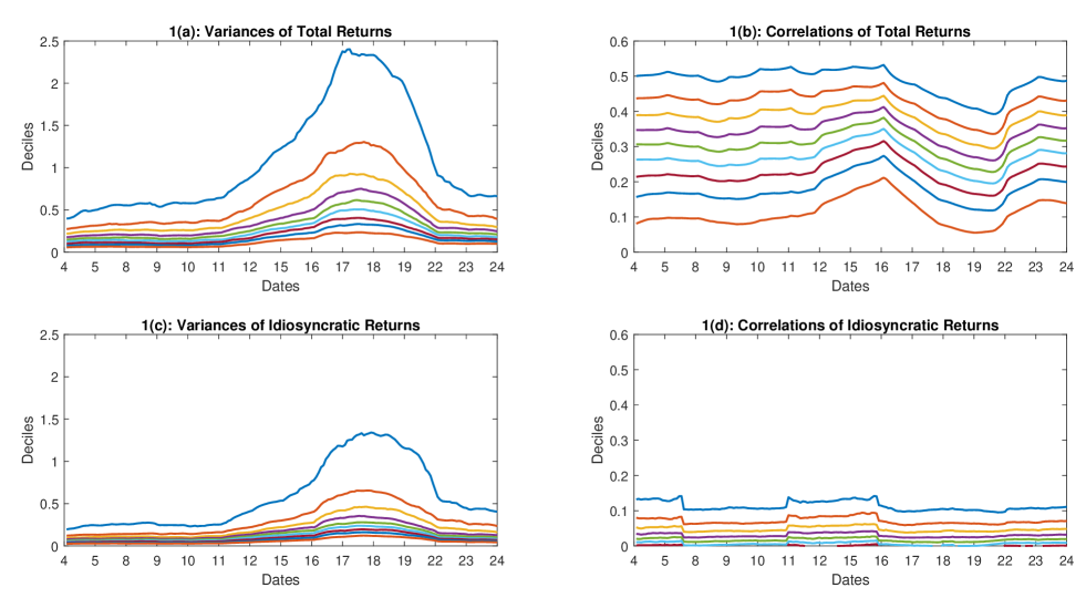
Figure 1: Deciles of spot variances and pairwise correlations in September 2008

To examine whether it is appropriate to directly apply shrinkage techniques to the spot volatility matrices of the total returns, following Fan, Furger and Xiu (2016) we plot in Figure 2(a) and (b) their sparsity patterns on the 16th and the 19th of September . The deep blue dots correspond to the locations of pairwise correlations that are at least $0.15$, whereas the white dots correspond to those smaller than $0.15$. Note that the covariance structure of the total returns is very dense on these two days. Therefore, it is not appropriate to directly apply the shrinkage technique as in Sections 2 and 3. Meanwhile, although both are quite dense, we can still clearly see their differences. Consistent with our observation from the decile plots of the correlations, we can see that the plot for the 16th is almost completely covered by blue dots, but the plot for the 19th in contrast has significantly more areas covered in white.

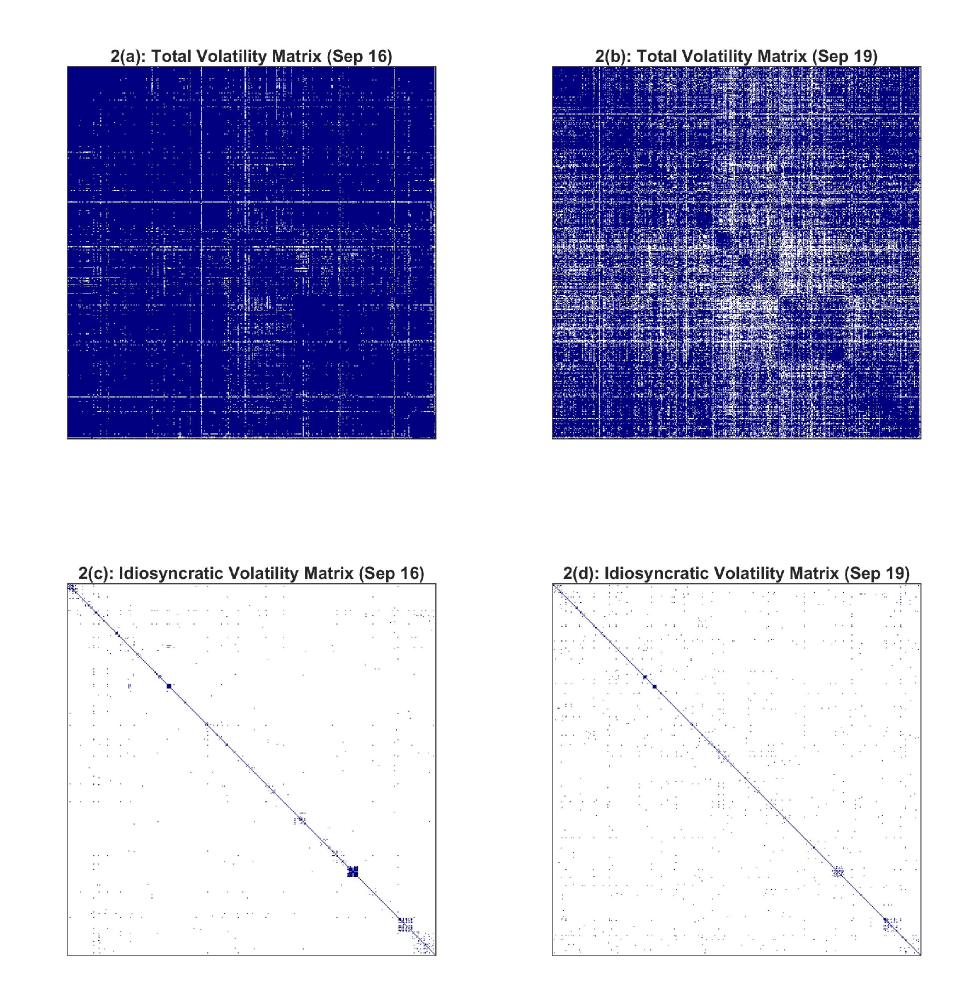
Figure 2: Sparsity patterns of the total and idiosyncratic volatility matrix estimates on September 16 and 19, 2008

We next incorporate the twelve observed factors in the large spot volatility matrix estimation as suggested in Section 4. In particular, we are interested on estimating the spot idiosyncratic volatility matrix, which is expected to satisfy the sparsity restriction. To save space, we choose to only report results using the SCAD shrinkage due to its satisfactory performance in our simulations. In Figure 1(c) and (d), we plot the deciles of the estimated spot idiosyncratic variances and correlations over trading days. In Figure 1(c), we observe a significant upward shift of the distribution of the spot variances of the idiosyncratic returns around the time of Lehman Brothers’ bankruptcy, indicating that the observed factors may not fully capture the time variation of the spot variances. In contrast, the deciles of the spot correlations in Figure 1(d) seem to be quite flat throughout the entire month, suggesting that the systematic factors may explain the time variation in the distribution of the pairwise correlations better than that of the variances.

We finally plot the sparsity patterns of the two estimated spot idiosyncratic volatility matrices on 16 and 19 September in Figure 2(c) and (d), respectively. Unlike Figure 2(a) and (b), we note that the estimated spot idiosyncratic volatility matrices are highly sparse on the two days. This is consistent with our observation from Figure 1(d), confirming that the observed factors can effectively account for the time variation in the spot covariance structure of the returns. Meanwhile, we also note that the two idiosyncratic volatility matrices are clearly not diagonal and still carry some visible time variation. Lastly, it is worth mentioning that the estimated spot idiosyncratic volatility matrices do not exhibit significant correlations within the blocks along the diagonal lines, except for some very limited actions in the lower right corner of the two matrices (the lower right corner corresponds to the XLU sector according to our sorting).

7 Conclusion

We developed nonparametric estimation methods for large spot volatility matrices under the uniform sparsity assumption. We allowed for microstructure noise and observed common risk factors and employed kernel smoothing and generalised shrinkage. In each scenario we obtained the uniform convergence rates for the large estimated covariance matrices and these reflect the smoothness and sparsity assumptions we made. The simulation results show that the proposed estimation methods work well in finite samples for both the noise-free and noise-contaminated data. The empirical study demonstrated the effectiveness on S&P 500 stocks five minute data. Several issues can be further explored. For example, it is worthwhile to further study the spot precision matrix estimation which is briefly discussed in Appendix C.1 of the supplement and explore its application to optimal portfolio choice.

Appendix A: Proofs of the main results

In this appendix, we give the proofs of the main theorems. We start with four propositions whose proofs are available in Appendix B of the supplement.

Proposition A.1.

Suppose that Assumptions 1 and 2(i)(ii) are satisfied. Then, we have

$$\max_{1\leq i,j\leq p}\sup_{0\leq t\leq T}\left|\widehat{\Sigma}_{ij,t}-\Sigma_{ij,t}\right|=O_{P}\left(\zeta_{\Delta,p}\right),$$ (A.1)

where $\zeta_{\Delta,p}=h^{\gamma}+\left[\frac{\Delta\log(p\vee\Delta^{-1})}{h}\right]^{1/2}$.

Proposition A.2.

Suppose that Assumptions 1, 2(i), 3 and 4(i)(ii) are satisfied, and Assumption 2(ii) holds with $\Delta^{-1}$ replaced by $N$.

$$\max_{1\leq i,j\leq p}\sup_{0\leq t\leq T}\left|\widetilde{\Sigma}_{ij,t}-\Sigma_{ij,t}\right|=O_{P}\left(\zeta_{N,p}^{\ast}+\nu_{\Delta,p,N}\right),$$ (A.2)

where $\zeta_{N,p}^{\ast}$ and $\nu_{\Delta,p,N}$ are defined in Assumption 4(iii).

Proposition A.3.

Suppose that Assumptions 1, 2(i), 3 and 5 are satisfied. Then, we have

$$\max_{1\leq i,j\leq p}\sup_{0\leq t\leq T}\left|\widehat{\Omega}_{ij}(t)-\Omega_{ij}(t)\right|=O_{P}\left(\delta_{\Delta,p}\right),$$ (A.3)

where $\delta_{\Delta,p}=h_{1}^{\gamma_{1}}+\left[\frac{\Delta\log(p\vee\Delta^{-1})}{h_{1}}\right]^{1/2}$.

Proposition A.4.

Suppose that Assumptions 2(i)(ii) and 6 are satisfied. Then, we have

$$\sup_{0\leq t\leq T}\left\|\widehat{\boldsymbol{\Sigma}}_{t}^{Y}-{\boldsymbol{\Sigma}}_{t}^{Y}\right\|_{\max}=O_{P}\left(\zeta_{\Delta,p}\right),$$

$$\sup_{0\leq t\leq T}\left\|\widehat{\boldsymbol{\Sigma}}_{t}^{F}-{\boldsymbol{\Sigma}}_{t}^{F}\right\|_{\max}=O_{P}\left(\zeta_{\Delta,p}\right),$$

$$\sup_{0\leq t\leq T}\left\|\widehat{\boldsymbol{\Sigma}}_{t}^{YF}-{\boldsymbol{\Sigma}}_{t}^{YF}\right\|_{\max}=O_{P}\left(\zeta_{\Delta,p}\right).$$

where $\zeta_{\Delta,p}$ is defined as in Proposition A.1.

Proof of Theorem 1. By the definition of $\widehat{\boldsymbol{\Sigma}}_{t}^{s}$ and the property of $s_{\rho}(\cdot)$, we readily have that

$$\sup_{0\leq t\leq T}\left\|\widehat{\boldsymbol{\Sigma}}_{t}^{s}-{\boldsymbol{\Sigma}}_{t}\right\| \leq \sup_{0\leq t\leq T}\max_{1\leq i\leq p}\sum_{j=1}^{p}\left|\widehat{\Sigma}_{ij,t}^{s}-\Sigma_{ij,t}\right|$$ (A.4)

$$= \sup_{0\leq t\leq T}\max_{1\leq i\leq p}\left|\widehat{\Sigma}_{ii,t}-\Sigma_{ii,t}\right|+\sup_{0\leq t\leq T}\max_{1\leq i\leq p}\sum_{j=1,\neq i}^{p}\left|s_{\rho_{1}(t)}\left(\widehat{\Sigma}_{ij,t}\right)I\left(\left|\widehat{\Sigma}_{ij,t}\right|>\rho_{1}(t)\right)-\Sigma_{ij,t}\right|$$

$$= \sup_{0\leq t\leq T}\max_{1\leq i\leq p}\left|\widehat{\Sigma}_{ii,t}-\Sigma_{ii,t}\right|+\sup_{0\leq t\leq T}\max_{1\leq i\leq p}\sum_{j=1,\neq i}^{p}\left|s_{\rho_{1}(t)}\left(\widehat{\Sigma}_{ij,t}\right)I\left(\left|\widehat{\Sigma}_{ij,t}\right|>\rho_{1}(t)\right)-\right.$$

$$\left.\Sigma_{ij,t}I\left(\left|\widehat{\Sigma}_{ij,t}\right|>\rho_{1}(t)\right)-\Sigma_{ij,t}I\left(\left|\widehat{\Sigma}_{ij,t}\right|\leq\rho_{1}(t)\right)\right|$$

$$\leq \sup_{0\leq t\leq T}\max_{1\leq i\leq p}\left|\widehat{\Sigma}_{ii,t}-\Sigma_{ii,t}\right|+\sup_{0\leq t\leq T}\max_{1\leq i\leq p}\sum_{j=1,\neq i}^{p}\left|s_{\rho_{1}(t)}\left(\widehat{\Sigma}_{ij,t}\right)-\widehat{\Sigma}_{ij,t}\right|I\left(\left|\widehat{\Sigma}_{ij,t}\right|>\rho_{1}(t)\right)+$$

$$\sup_{0\leq t\leq T}\max_{1\leq i\leq p}\sum_{j=1,\neq i}^{p}\left|\widehat{\Sigma}_{ij,t}-\Sigma_{ij,t}\right|I\left(\left|\widehat{\Sigma}_{ij,t}\right|>\rho_{1}(t)\right)+\sup_{0\leq t\leq T}\max_{1\leq i\leq p}\sum_{j=1,\neq i}^{p}\left|\Sigma_{ij,t}\right|I\left(\left|\widehat{\Sigma}_{ij,t}\right|\leq\rho_{1}(t)\right)$$

$$=: \Pi_{1}+\Pi_{2}+\Pi_{3}+\Pi_{4}.$$

Define the event

$$\mathcal{G}(M)=\left\{\max_{1\leq i,j\leq p}\sup_{0\leq t\leq T}\left|\widehat{\Sigma}_{ij,t}-\Sigma_{ij,t}\right|\leq M\zeta_{\Delta,p}\right\}$$

where $M$ is a positive constant. For any small $\epsilon>0$, by (A.1), we may find a sufficiently large constant $M_{\epsilon}>0$ such that

$$\mathsf{P}\left(\mathcal{G}(M_{\epsilon})\right)\geq 1-\epsilon.$$ (A.5)

By property (iii) of the shrinkage function and (A.5), we have

$$\Pi_{2}\leq\sup_{0\leq t\leq T}\rho_{1}(t)\left[\max_{1\leq i\leq p}\sum_{j=1}^{p}I\left(\left|\widehat{\Sigma}_{ij,t}\right|>\rho_{1}(t)\right)\right]$$

and

$$\Pi_{3}\leq M_{\epsilon}\zeta_{\Delta,p}\left[\sup_{0\leq t\leq T}\max_{1\leq i\leq p}\sum_{j=1}^{p}I\left(\left|\widehat{\Sigma}_{ij,t}\right|>\rho_{1}(t)\right)\right]$$

conditional on the event $\mathcal{G}(M_{\epsilon})$. By the reverse triangle inequality and Proposition A.1,

$$\left|\widehat{\Sigma}_{ij,t}\right|\leq\left|\Sigma_{ij,t}\right|+M_{\epsilon}\zeta_{\Delta,p}$$

on $\mathcal{G}(M_{\epsilon})$. Letting $\underline{C}_{M}=2M_{\epsilon}$ in Assumption 2(iii), as $\left\{{\boldsymbol{\Sigma}}_{t}:\ 0\leq t\leq T\right\}\in\mathcal{S}(q,\varpi(p),T)$, we have

$$\Pi_{2}+\Pi_{3} \leq \zeta_{\Delta,p}(\overline{C}_{M}+M_{\epsilon})\left[\sup_{0\leq t\leq T}\max_{1\leq i\leq p}\sum_{j=1}^{p}I\left(\left|\widehat{\Sigma}_{ij,t}\right|>\underline{C}_{M}\zeta_{\Delta,p}\right)\right]$$ (A.6)

$$\leq \zeta_{\Delta,p}(\overline{C}_{M}+M_{\epsilon})\left[\sup_{0\leq t\leq T}\max_{1\leq i\leq p}\sum_{j=1}^{p}I\left(\left|\widehat{\Sigma}_{ij,t}\right|>M_{\epsilon}\zeta_{\Delta,p}\right)\right]$$

$$= O_{P}\left(\zeta_{\Delta,p}\right)\left[\sup_{0\leq t\leq T}\max_{1\leq i\leq p}\sum_{j=1}^{p}\frac{|\Sigma_{ij,t}|^{q}}{\left(M_{\epsilon}\zeta_{\Delta,p}\right)^{q}}\right]$$

$$= O_{P}\left(\Lambda\varpi(p)\zeta_{\Delta,p}^{1-q}\right)=O_{P}\left(\varpi(p)\zeta_{\Delta,p}^{1-q}\right).$$

on the event $\mathcal{G}(M_{\epsilon})$, where $\overline{C}_{M}$ is defined in Assumption 2(iii). Note that the events $\left\{\left|\widehat{\Sigma}_{ij,t}\right|\leq\rho_{1}(t)\right\}$ and $\mathcal{G}(M_{\epsilon})$ jointly imply that $\left\{|\Sigma_{ij,t}|\leq\left(\overline{C}_{M}+M_{\epsilon}\right)\zeta_{\Delta,p}\right\}$. Then, we may show that

$$\Pi_{4} \leq \sup_{0\leq t\leq T}\max_{1\leq i\leq p}\sum_{j=1}^{p}|\Sigma_{ij,t}|I\left(|\Sigma_{ij,t}|\leq\left(\overline{C}_{M}+M_{\epsilon}\right)\zeta_{\Delta,p}\right)$$ (A.7)

$$\leq \left(\overline{C}_{M}+M_{\epsilon}\right)^{1-q}\zeta_{\Delta,p}^{1-q}\sup_{0\leq t\leq T}\max_{1\leq i\leq p}\sum_{j=1}^{p}|\Sigma_{ij,t}|^{q}$$

$$= O_{P}\left(\Lambda\varpi(p)\zeta_{\Delta,p}^{1-q}\right)=O_{P}\left(\varpi(p)\zeta_{\Delta,p}^{1-q}\right).$$

By Proposition A.1, we readily have that

$$\Pi_{1}=O_{P}\left(\zeta_{\Delta,p}\right)=O_{P}\left(\varpi(p)\zeta_{\Delta,p}^{1-q}\right).$$ (A.8)

By (A.6)–(A.8), and letting $\epsilon\rightarrow 0$ in (A.5), we complete the proof of Theorem 1. $\blacksquare$

Proof of Theorem 2.  The proof is similar to the proof of Theorem 1 with Proposition A.2 replacing Proposition A.1. Details are omitted to save the space. $\blacksquare$

Proof of Theorem 3.  The proof is similar to the proof of Theorem 1 with Proposition A.3 replacing Proposition A.1. Details are omitted to save the space. $\blacksquare$

Proof of Theorem 4.  By Proposition A.4 and the definition of $\widehat{\Sigma}_{ij,t}^{X}$ in (4.8), we may show that

$$\max_{1\leq i,j\leq p}\sup_{0\leq t\leq T}\left|\widehat{\Sigma}_{ij,t}^{X}-\Sigma_{ij,t}^{X}\right|=O_{P}\left(\zeta_{\Delta,p}\right).$$ (A.9)

With (A.9), following the proof of Theorem 1, we complete the proof of (4.12).

We next turn to the proof of (4.13). Note that

$$\sup_{0\leq t\leq T}\left\|\widehat{\boldsymbol{\Sigma}}_{t}^{Y,s}-{\boldsymbol{\Sigma}}_{t}^{Y}\right\|_{{\boldsymbol{\Sigma}}_{t}^{Y}}^{2}\leq 2\sup_{0\leq t\leq T}\left[\left\|\widehat{\boldsymbol{\Sigma}}_{t}^{X,s}-{\boldsymbol{\Sigma}}_{t}^{X}\right\|_{{\boldsymbol{\Sigma}}_{t}^{Y}}^{2}+\left\|\widehat{\boldsymbol{\beta}}(t)\widehat{\boldsymbol{\Sigma}}_{t}^{F}\widehat{\boldsymbol{\beta}}(t)^{{}^{\intercal}}-{\boldsymbol{\beta}}(t){\boldsymbol{\Sigma}}_{t}^{F}{\boldsymbol{\beta}}(t)^{{}^{\intercal}}\right\|_{{\boldsymbol{\Sigma}}_{t}^{Y}}^{2}\right].$$

For any $p\times p$ matrix ${\boldsymbol{\Sigma}}$, since all the eigenvalues of ${\boldsymbol{\Sigma}}_{t}^{Y}$ are strictly larger than a positive constant,

$$\|{\boldsymbol{\Sigma}}\|_{{\boldsymbol{\Sigma}}_{t}^{Y}}^{2}=\frac{1}{p}\left\|\left({\boldsymbol{\Sigma}}_{t}^{Y}\right)^{-1/2}{\boldsymbol{\Sigma}}\left({\boldsymbol{\Sigma}}_{t}^{Y}\right)^{-1/2}\right\|_{F}^{2}\leq\frac{C}{p}\|{\boldsymbol{\Sigma}}\|_{F}^{2},$$ (A.10)

where $C>0$ is a generic constant whose value may change from line to line. By (4.12) and (A.10), we prove

$$\sup_{0\leq t\leq T}\left\|\widehat{\boldsymbol{\Sigma}}_{t}^{X,s}-{\boldsymbol{\Sigma}}_{t}^{X}\right\|_{{\boldsymbol{\Sigma}}_{t}^{Y}}^{2}\leq\frac{C}{p}\sup_{0\leq t\leq T}\left\|\widehat{\boldsymbol{\Sigma}}_{t}^{X,s}-{\boldsymbol{\Sigma}}_{t}^{X}\right\|_{F}^{2}\leq C\sup_{0\leq t\leq T}\left\|\widehat{\boldsymbol{\Sigma}}_{t}^{X,s}-{\boldsymbol{\Sigma}}_{t}^{X}\right\|^{2}=O_{P}\left([\varpi(p)\zeta_{\Delta,p}^{1-q}]^{2}\right).$$ (A.11)

By the definition of $\widehat{\boldsymbol{\beta}}(t)$ in (4.7) and Proposition A.4, we readily have that

$$\max_{1\leq i\leq p}\sup_{0\leq t\leq T}\left\|\widehat{\beta}_{i}(t)-\beta_{i}(t)\right\|_{2}=O_{P}\left(\zeta_{\Delta,p}\right).$$ (A.12)

Write ${\mathbf{D}}_{t}^{\beta}=\widehat{\boldsymbol{\beta}}(t)-{\boldsymbol{\beta}}(t)$ and ${\mathbf{D}}_{t}^{F}=\widehat{\boldsymbol{\Sigma}}_{t}^{F}-{\boldsymbol{\Sigma}}_{t}^{F}$. Note that

$$\widehat{\boldsymbol{\beta}}(t)\widehat{\boldsymbol{\Sigma}}_{t}^{F}\widehat{\boldsymbol{\beta}}(t)^{{}^{\intercal}}-{\boldsymbol{\beta}}(t){\boldsymbol{\Sigma}}_{t}^{F}{\boldsymbol{\beta}}(t)^{{}^{\intercal}} = {\mathbf{D}}_{t}^{\beta}{\mathbf{D}}_{t}^{F}{\mathbf{D}}_{t}^{\beta{{}^{\intercal}}}+{\mathbf{D}}_{t}^{\beta}{\boldsymbol{\Sigma}}_{t}^{F}{\mathbf{D}}_{t}^{\beta{{}^{\intercal}}}+{\mathbf{D}}_{t}^{\beta}{\mathbf{D}}_{t}^{F}{\boldsymbol{\beta}}(t)^{{}^{\intercal}}+$$

$${\mathbf{D}}_{t}^{\beta}{\boldsymbol{\Sigma}}_{t}^{F}{\boldsymbol{\beta}}(t)^{{}^{\intercal}}+{\boldsymbol{\beta}}(t){\mathbf{D}}_{t}^{F}{\mathbf{D}}_{t}^{\beta{{}^{\intercal}}}+{\boldsymbol{\beta}}(t){\boldsymbol{\Sigma}}_{t}^{F}{\mathbf{D}}_{t}^{\beta{{}^{\intercal}}}+{\boldsymbol{\beta}}(t){\mathbf{D}}_{t}^{F}{\boldsymbol{\beta}}(t)^{{}^{\intercal}}.$$

By (A.10), (A.12) and Proposition A.4, we have

$$\sup_{0\leq t\leq T}\left\|{\mathbf{D}}_{t}^{\beta}{\mathbf{D}}_{t}^{F}{\mathbf{D}}_{t}^{\beta{{}^{\intercal}}}\right\|_{{\boldsymbol{\Sigma}}_{t}^{Y}}^{2} \leq C\sup_{0\leq t\leq T}\frac{1}{p}\left\|{\mathbf{D}}_{t}^{\beta}{\mathbf{D}}_{t}^{F}{\mathbf{D}}_{t}^{\beta{{}^{\intercal}}}\right\|_{F}^{2}$$ (A.13)

$$\leq \frac{C}{p}\sup_{0\leq t\leq T}\left\|{\mathbf{D}}_{t}^{\beta}\right\|_{F}^{4}\sup_{0\leq t\leq T}\left\|{\mathbf{D}}_{t}^{F}\right\|^{2}$$

$$= O_{P}\left(p\zeta_{\Delta,p}^{6}\right).$$

Similarly, we can show that

$$\sup_{0\leq t\leq T}\left\|{\mathbf{D}}_{t}^{\beta}{\boldsymbol{\Sigma}}_{t}^{F}{\mathbf{D}}_{t}^{\beta{{}^{\intercal}}}\right\|_{{\boldsymbol{\Sigma}}_{t}^{Y}}^{2}\leq C\sup_{0\leq t\leq T}\frac{1}{p}\left\|{\mathbf{D}}_{t}^{\beta}\right\|_{F}^{4}=O_{P}\left(p\zeta_{\Delta,p}^{4}\right).$$ (A.14)

By (4.3), Assumption 6(iv) and Sherman-Morrison-Woodbury formula, we may show that

$$\sup_{0\leq t\leq T}\left\|{\boldsymbol{\beta}}(t)^{{}^{\intercal}}\left({\boldsymbol{\Sigma}}_{t}^{Y}\right)^{-1}{\boldsymbol{\beta}}(t)\right\|=O_{P}(1).$$ (A.15)

Using (A.12), (A.15) and Proposition A.4, we have

$$\sup_{0\leq t\leq T}\left\|{\mathbf{D}}_{t}^{\beta}{\mathbf{D}}_{t}^{F}{\boldsymbol{\beta}}(t)^{{}^{\intercal}}\right\|_{{\boldsymbol{\Sigma}}_{t}^{Y}}^{2} = \frac{1}{p}\sup_{0\leq t\leq T}{\sf trace}\left\{{\mathbf{D}}_{t}^{F}{\mathbf{D}}_{t}^{\beta{{}^{\intercal}}}\left({\boldsymbol{\Sigma}}_{t}^{Y}\right)^{-1}{\mathbf{D}}_{t}^{\beta}{\mathbf{D}}_{t}^{F}{\boldsymbol{\beta}}(t)^{{}^{\intercal}}\left({\boldsymbol{\Sigma}}_{t}^{Y}\right)^{-1}{\boldsymbol{\beta}}(t)\right\}$$ (A.16)

$$\leq \frac{C}{p}\sup_{0\leq t\leq T}\left\|{\mathbf{D}}_{t}^{\beta}\right\|_{F}^{2}\sup_{0\leq t\leq T}\left\|{\mathbf{D}}_{t}^{F}\right\|^{2}\sup_{0\leq t\leq T}\left\|{\boldsymbol{\beta}}(t)^{{}^{\intercal}}\left({\boldsymbol{\Sigma}}_{t}^{Y}\right)^{-1}{\boldsymbol{\beta}}(t)\right\|$$

$$\leq \frac{C}{p}\sup_{0\leq t\leq T}\left\|{\mathbf{D}}_{t}^{\beta}\right\|_{F}^{2}\sup_{0\leq t\leq T}\left\|{\mathbf{D}}_{t}^{F}\right\|^{2}=O_{P}\left(\zeta_{\Delta,p}^{4}\right),$$

and

$$\sup_{0\leq t\leq T}\left\|{\boldsymbol{\beta}}(t){\mathbf{D}}_{t}^{F}{\mathbf{D}}_{t}^{\beta{{}^{\intercal}}}\right\|_{{\boldsymbol{\Sigma}}_{t}^{Y}}^{2}=O_{P}\left(\zeta_{\Delta,p}^{4}\right).$$ (A.17)

Similar to the proof of (A.16), we also have

$$\sup_{0\leq t\leq T}\left\|{\mathbf{D}}_{t}^{\beta}{\boldsymbol{\Sigma}}_{t}^{F}{\boldsymbol{\beta}}(t)^{{}^{\intercal}}\right\|_{{\boldsymbol{\Sigma}}_{t}^{Y}}^{2}\leq\frac{C}{p}\sup_{0\leq t\leq T}\left\|{\mathbf{D}}_{t}^{\beta}\right\|_{F}^{2}\sup_{0\leq t\leq T}\left\|{\boldsymbol{\Sigma}}_{t}^{F}\right\|^{2}=O_{P}\left(\zeta_{\Delta,p}^{2}\right),$$ (A.18)

and

$$\sup_{0\leq t\leq T}\left\|{\boldsymbol{\beta}}(t){\boldsymbol{\Sigma}}_{t}^{F}{\mathbf{D}}_{t}^{\beta{{}^{\intercal}}}\right\|_{{\boldsymbol{\Sigma}}_{t}^{Y}}^{2}=O_{P}\left(\zeta_{\Delta,p}^{2}\right).$$ (A.19)

By (A.15) and Proposition A.4, we may show that

$$\sup_{0\leq t\leq T}\left\|{\boldsymbol{\beta}}(t){\mathbf{D}}_{t}^{F}{\boldsymbol{\beta}}(t)^{{}^{\intercal}}\right\|_{{\boldsymbol{\Sigma}}_{t}^{Y}}^{2} = \frac{1}{p}\sup_{0\leq t\leq T}{\sf trace}\left\{{\mathbf{D}}_{t}^{F}{\boldsymbol{\beta}}(t)^{{}^{\intercal}}\left({\boldsymbol{\Sigma}}_{t}^{Y}\right)^{-1}{\boldsymbol{\beta}}(t){\mathbf{D}}_{t}^{F}{\boldsymbol{\beta}}(t)^{{}^{\intercal}}\left({\boldsymbol{\Sigma}}_{t}^{Y}\right)^{-1}{\boldsymbol{\beta}}(t)\right\}$$ (A.20)

$$\leq \frac{C}{p}\sup_{0\leq t\leq T}\left\|{\mathbf{D}}_{t}^{F}\right\|^{2}\sup_{0\leq t\leq T}\left\|{\boldsymbol{\beta}}(t)^{{}^{\intercal}}\left({\boldsymbol{\Sigma}}_{t}^{Y}\right)^{-1}{\boldsymbol{\beta}}(t)\right\|^{2}=O_{P}\left(\zeta_{\Delta,p}^{2}/p\right).$$

With (A.13), (A.14) and (A.16)–(A.20), we have

$$\sup_{0\leq t\leq T}\left\|\widehat{\boldsymbol{\beta}}(t)\widehat{\boldsymbol{\Sigma}}_{t}^{F}\widehat{\boldsymbol{\beta}}(t)^{{}^{\intercal}}-{\boldsymbol{\beta}}(t){\boldsymbol{\Sigma}}_{t}^{F}{\boldsymbol{\beta}}(t)^{{}^{\intercal}}\right\|_{{\boldsymbol{\Sigma}}_{t}^{Y}}^{2}=O_{P}\left(p\zeta_{\Delta,p}^{4}+\zeta_{\Delta,p}^{2}\right).$$ (A.21)

By virtue of (A.11) and (A.21), we complete the proof of (4.13). $\blacksquare$

Supplement to “Nonparametric Estimation of Large Spot Volatility Matrices for High-Frequency Financial Data”

In this supplement, we provide the detailed proofs of the propositions stated in Appendix A, discuss the spot precision matrix estimation, address the asynchronicity issue and report additional simulation results.

Appendix B: Proofs of technical results

As discussed in Remark 1, the local boundedness condition in Assumption 1(i) can be strengthened to the following uniform boundedness condition:

$$\max_{1\leq i\leq p}\sup_{0\leq s\leq T}|\mu_{i,s}|\leq C_{\mu}<\infty,\ \ \max_{1\leq i\leq p}\sup_{0\leq s\leq T}\Sigma_{ii,t}\leq C_{\Sigma}<\infty,$$ (B.1)

with probability one. Throughout this appendix, we let $C$ denote a generic positive constant whose value may change from line to line.

Proof of Proposition A.1. Throughout this proof, we let $\zeta_{\Delta,p}^{\ast}=\left[\frac{\Delta\log(p\vee\Delta^{-1})}{h}\right]^{1/2}$. By (2.1), we have

$$(\Delta X_{i,k})(\Delta X_{j,k}) = \left(\int_{t_{k-1}}^{t_{k}}\mu_{i,s}ds+\sum_{l=1}^{p}\int_{t_{k-1}}^{t_{k}}\sigma_{il,s}dW_{l,s}\right)\left(\int_{t_{k-1}}^{t_{k}}\mu_{j,u}du+\sum_{l=1}^{p}\int_{t_{k-1}}^{t_{k}}\sigma_{jl,u}dW_{l,u}\right)$$

$$= \left(\int_{t_{k-1}}^{t_{k}}\mu_{i,s}ds\int_{t_{k-1}}^{t_{k}}\mu_{j,u}du\right)+\left(\int_{t_{k-1}}^{t_{k}}\sum_{l=1}^{p}\sigma_{il,s}dW_{l,s}\int_{t_{k-1}}^{t_{k}}\mu_{j,u}du\right)+$$

$$\left(\int_{t_{k-1}}^{t_{k}}\mu_{i,s}ds\int_{t_{k-1}}^{t_{k}}\sum_{l=1}^{p}\sigma_{jl,u}dW_{l,u}\right)+\left(\int_{t_{k-1}}^{t_{k}}\sum_{l=1}^{p}\sigma_{il,s}dW_{l,s}\int_{t_{k-1}}^{t_{k}}\sum_{l=1}^{p}\sigma_{jl,u}dW_{l,u}\right)$$

$$= M_{ij,k}(1)+M_{ij,k}(2)+M_{ij,k}(3)+M_{ij,k}(4).$$

This leads to the following decomposition:

$$\sum_{k=1}^{n}K_{h}(t_{k}-t)\Delta X_{i,k}\Delta X_{j,k} = \sum_{k=1}^{n}K_{h}(t_{k}-t)M_{ij,k}(1)+\sum_{k=1}^{n}K_{h}(t_{k}-t)M_{ij,k}(2)+$$

$$\sum_{k=1}^{n}K_{h}(t_{k}-t)M_{ij,k}(3)+\sum_{k=1}^{n}K_{h}(t_{k}-t)M_{ij,k}(4).$$

By (B.1) and Assumption 2(i)(ii), we readily have that

$$\max_{1\leq i,j\leq p}\sup_{0\leq t\leq T}\left|\sum_{k=1}^{n}K_{h}(t_{k}-t)M_{ij,k}(1)\right| \leq \max_{1\leq i,j\leq p}\max_{1\leq k\leq n}|M_{ij,k}(1)|\sup_{0\leq t\leq T}\sum_{k=1}^{n}K_{h}(t_{k}-t)$$ (B.2)

$$\leq C\Delta\sup_{0\leq t\leq T}\Delta\sum_{k=1}^{n}K_{h}(t_{k}-t)$$

$$= O_{P}\left(\Delta\right)=o_{P}\left(\zeta_{\Delta,p}^{\ast}\right),$$

as $\Delta\sum_{k=1}^{n}K_{h}(t_{k}-t)$ is bounded uniformly over $t$.

We next show that

$$\max_{1\leq i,j\leq p}\sup_{0\leq t\leq T}\left|\sum_{k=1}^{n}K_{h}(t_{k}-t)M_{ij,k}(4)-\sum_{k=1}^{n}K_{h}(t_{k}-t)\int_{t_{k-1}}^{t_{k}}\Sigma_{ij,s}ds\right|=O_{P}\left(\zeta_{\Delta,p}^{\ast}\right).$$ (B.3)

Let $dX_{i,t}^{\ast}=\sum_{l=1}^{p}\sigma_{il,t}dW_{l,t}$, $\Delta X_{i,k}^{\ast}=\int_{t_{k-1}}^{t_{k}}\sum_{l=1}^{p}\sigma_{il,s}dW_{l,s}=X_{i,t_{k}}^{\ast}-X_{i,t_{k-1}}^{\ast}$ and $X_{i,t}^{\ast}$ be adapted to the underlying filtration $(\mathcal{F}_{t})_{t\geq 0}$. Note that

$$M_{ij,k}(4) = \Delta X_{i,k}^{\ast}\Delta X_{j,k}^{\ast}=\frac{1}{2}\left[\left(\Delta X_{i,k}^{\ast}+\Delta X_{j,k}^{\ast}\right)\left(\Delta X_{i,k}^{\ast}+\Delta X_{j,k}^{\ast}\right)-\left(\Delta X_{i,k}^{\ast}\right)^{2}-\left(\Delta X_{j,k}^{\ast}\right)^{2}\right]$$

$$=: \frac{1}{2}\left[M_{ij,k}^{\ast}(4)-\left(\Delta X_{i,k}^{\ast}\right)^{2}-\left(\Delta X_{j,k}^{\ast}\right)^{2}\right].$$

Hence, to show (B.3), it is sufficient to prove that

$$\max_{1\leq i\leq p}\sup_{0\leq t\leq T}\left|\sum_{k=1}^{n}K_{h}(t_{k}-t)\left(\Delta X_{i,k}^{\ast}\right)^{2}-\sum_{k=1}^{n}K_{h}(t_{k}-t)\int_{t_{k-1}}^{t_{k}}\Sigma_{ii,s}ds\right|=O_{P}\left(\zeta_{\Delta,p}^{\ast}\right)$$ (B.4)

and

$$\max_{1\leq i,j\leq p}\sup_{0\leq t\leq T}\left|\sum_{k=1}^{n}K_{h}(t_{k}-t)M_{ij,k}^{\ast}(4)-\sum_{k=1}^{n}K_{h}(t_{k}-t)\int_{t_{k-1}}^{t_{k}}\Sigma_{ij,s}^{\ast}ds\right|=O_{P}\left(\zeta_{\Delta,p}^{\ast}\right),$$ (B.5)

where $\Sigma_{ij,s}^{\ast}$ is defined in Assumption 1(ii).

We next only prove (B.4) as the proof of (B.5) is analogous. Consider covering the interval $[0,T]$ by some disjoint intervals $\mathcal{T}_{v}$ with centre $\tau_{v}^{\ast}$ and length $d=h^{2}\zeta_{\Delta,p}^{\ast}$, $v=1,2,\cdots,V$. Observe that

$$\max_{1\leq i\leq p}\sup_{0\leq t\leq T}\left|\sum_{k=1}^{n}K_{h}(t_{k}-t)\left(\Delta X_{i,k}^{\ast}\right)^{2}-\sum_{k=1}^{n}K_{h}(t_{k}-t)\int_{t_{k-1}}^{t_{k}}\Sigma_{ii,s}ds\right|$$ (B.6)

$$\leq \max_{1\leq i\leq p}\max_{1\leq v\leq V}\left|\sum_{k=1}^{n}K_{h}(t_{k}-\tau_{v}^{\ast})\left(\Delta X_{i,k}^{\ast}\right)^{2}-\sum_{k=1}^{n}K_{h}(t_{k}-\tau_{v}^{\ast})\int_{t_{k-1}}^{t_{k}}\Sigma_{ii,s}ds\right|+$$

$$\max_{1\leq i\leq p}\max_{1\leq v\leq V}\sup_{t\in\mathcal{T}_{v}}\left|\sum_{k=1}^{n}\left[K_{h}(t_{k}-t)-K_{h}(t_{k}-\tau_{v}^{\ast})\right]\left(\Delta X_{i,k}^{\ast}\right)^{2}\right|+$$

$$\max_{1\leq i\leq p}\max_{1\leq v\leq V}\sup_{t\in\mathcal{T}_{v}}\left|\sum_{k=1}^{n}\left[K_{h}(t_{k}-t)-K_{h}(t_{k}-\tau_{v}^{\ast})\right]\int_{t_{k-1}}^{t_{k}}\Sigma_{ii,s}ds\right|.$$

As the kernel function has the compact support $[-1,1]$, we have, for any $t\in[0,T]$,

$$\sum_{k=1}^{n}K_{h}(t_{k}-t)\left[\left(\Delta X_{i,k}^{\ast}\right)^{2}-\int_{t_{k-1}}^{t_{k}}\Sigma_{ii,s}ds\right]=\sum_{k=l(t)}^{u(t)}K_{h}(t_{k}-t)\left[\left(\Delta X_{i,k}^{\ast}\right)^{2}-\int_{t_{k-1}}^{t_{k}}\Sigma_{ii,s}ds\right],$$

where $l(t)=\lfloor(t-h)/\Delta\rfloor\vee 1$ and $u(t)=\lfloor(t+h)/\Delta\rfloor\wedge n$. Letting $\mathcal{N}$ be a standard normal random variable, by Lemma 1 in Fan, Li and Yu (2012), we have

$$\mathsf{E}\left(\exp\{\psi(\mathcal{N}^{2}-1)\}\right)\leq\exp\left\{2\psi^{2}\right\}\ \ \mathrm{for}\ |\psi|\leq 1/4.$$ (B.7)

Following the argument in the proof of Lemma 3 in Fan, Li and Yu (2012) and using (B.7), for $k=l(\tau_{v}^{\ast}),l(\tau_{v}^{\ast})+1,\cdots,u(\tau_{v}^{\ast})$,

$$\mathsf{E}\left(\exp\left\{\theta\left(\Delta^{-1}h\right)^{1/2}K_{h}(t_{k}-\tau_{v}^{\ast})\left[\left(\Delta X_{i,k}^{\ast}\right)^{2}-\int_{t_{k-1}}^{t_{k}}\Sigma_{ii,s}ds\right]\right\}|\mathcal{F}_{t_{k-1}}\right)$$

$$\leq \exp\left\{\frac{2\Delta}{h}\theta^{2}C_{\Sigma}^{2}K^{2}\left(\frac{t_{k}-\tau_{v}^{\ast}}{h}\right)\right\},$$

where $\theta$ satisfies that $\left|\theta C_{\Sigma}(\Delta h^{-1})^{1/2}K\left(\frac{t_{k}-\tau_{v}^{\ast}}{h}\right)\right|\leq 1/4$ and $C_{\Sigma}$ is defined in (B.1). Consequently, we have

$$\mathsf{E}\left(\exp\left\{\theta\left(\Delta^{-1}h\right)^{1/2}\sum_{k=1}^{n}K_{h}(t_{k}-\tau_{v}^{\ast})\left[\left(\Delta X_{i,k}^{\ast}\right)^{2}-\int_{t_{k-1}}^{t_{k}}\Sigma_{ii,s}ds\right]\right\}\right)$$ (B.8)

$$= \mathsf{E}\left(\exp\left\{\theta\left(\Delta^{-1}h\right)^{1/2}\sum_{k=l(\tau_{v}^{\ast})}^{u(\tau_{v}^{\ast})}K_{h}(t_{k}-\tau_{v}^{\ast})\left[\left(\Delta X_{i,k}^{\ast}\right)^{2}-\int_{t_{k-1}}^{t_{k}}\Sigma_{ii,s}ds\right]\right\}\right)$$

$$\leq \exp\left\{2\theta^{2}C_{\Sigma}^{2}\nu(\tau_{v}^{\ast})\right\},$$

where $\nu(\tau_{v}^{\ast})=(\Delta/h)\sum_{k=l(\tau_{v}^{\ast})}^{u(\tau_{v}^{\ast})}K^{2}(t_{k}-\tau_{v}^{\ast})$. By (B.8), using the Markov inequality and choosing $\theta=\frac{\sqrt{\log(p\vee\Delta^{-1})}}{C_{\Sigma}^{2}\nu(\tau_{v}^{\ast})}$, we can prove that

$$\mathsf{P}\left(\left|\sum_{k=1}^{n}K_{h}(t_{k}-\tau_{v}^{\ast})\left(\Delta X_{i,k}^{\ast}\right)^{2}-\sum_{k=1}^{n}K_{h}(t_{k}-\tau_{v}^{\ast})\int_{t_{k-1}}^{t_{k}}\Sigma_{ii,s}ds\right|>M\zeta_{\Delta,p}^{\ast}\right)\leq 2\exp\{-C(M)\log(p\vee\Delta^{-1})\},$$

where $C(M)$ is positive and becomes sufficiently large if we choose $M$ to be large enough. Then, by the Bonferroni inequality, we have

$$\mathsf{P}\left(\max_{1\leq i\leq p}\max_{1\leq v\leq V}\left|\sum_{k=1}^{n}K_{h}(t_{k}-\tau_{v}^{\ast})\left(\Delta X_{i,k}^{\ast}\right)^{2}-\sum_{k=1}^{n}K_{h}(t_{k}-\tau_{v}^{\ast})\int_{t_{k-1}}^{t_{k}}\Sigma_{ii,s}ds\right|>M\zeta_{\Delta,p}^{\ast}\right)$$

$$\leq \sum_{i=1}^{p}\sum_{v=1}^{V}2\exp\{-C(M)(\log(p\vee\Delta^{-1}))\}\rightarrow 0,$$

where the convergence is due to the fact $pV=o\left(\exp\{C_{M}\log(p\vee\Delta^{-1})\}\right)$ as $V$ is divergent at a polynomial rate of $1/\Delta$ and $C(M)$ is sufficiently large, which implies that

$$\max_{1\leq i\leq p}\max_{1\leq v\leq V}\left|\sum_{k=1}^{n}K_{h}(t_{k}-\tau_{v}^{\ast})\left(\Delta X_{i,k}^{\ast}\right)^{2}-\sum_{k=1}^{n}K_{h}(t_{k}-\tau_{v}^{\ast})\int_{t_{k-1}}^{t_{k}}\Sigma_{ii,s}ds\right|=O_{P}(\zeta_{\Delta,p}^{\ast}).$$ (B.9)

By the smoothness condition on the kernel function in Assumption 2(i), we have

$$\max_{1\leq i\leq p}\max_{1\leq v\leq V}\sup_{t\in\mathcal{T}_{v}}\left|\sum_{k=1}^{n}\left[K_{h}(t_{k}-t)-K_{h}(t_{k}-\tau_{v}^{\ast})\right]\left(\Delta X_{i,k}^{\ast}\right)^{2}\right|$$

$$\leq \max_{1\leq v\leq V}\sup_{t\in\mathcal{T}_{v}}\left|K_{h}(t_{k}-t)-K_{h}(t_{k}-\tau_{v}^{\ast})\right|\max_{1\leq i\leq p}\sum_{k=1}^{n}\left(\Delta X_{i,k}^{\ast}\right)^{2}$$

$$= O\left(dh^{-2}\right)\max_{1\leq i\leq p}\sum_{k=1}^{n}\left(\Delta X_{i,k}^{\ast}\right)^{2}.$$

Similar to the proof of (B.9), we may show that

$$\max_{1\leq i\leq p}\sum_{k=1}^{n}\left(\Delta X_{i,k}^{\ast}\right)^{2}\leq\max_{1\leq i\leq p}\int_{0}^{T}\Sigma_{ii,s}ds+o_{P}(1)=O_{P}(1)$$

as $T$ is fixed and $\Sigma_{ii,t}$ is uniformly bounded by $C_{\Sigma}$. Hence, by the choice of $d$, we have

$$\max_{1\leq i\leq p}\max_{1\leq v\leq V}\sup_{t\in\mathcal{T}_{v}}\left|\sum_{k=1}^{n}\left[K_{h}(t_{k}-t)-K_{h}(t_{k}-\tau_{v}^{\ast})\right]\left(\Delta X_{i,k}^{\ast}\right)^{2}\right|=O_{P}(\zeta_{\Delta,p}^{\ast}).$$ (B.10)

Analogously, we also have

$$\max_{1\leq i\leq p}\max_{1\leq v\leq V}\sup_{t\in\mathcal{T}_{v}}\left|\sum_{k=1}^{n}\left[K_{h}(t_{k}-t)-K_{h}(t_{k}-\tau_{v}^{\ast})\right]\int_{t_{k-1}}^{t_{k}}\Sigma_{ii,s}ds\right|=O_{P}(\zeta_{\Delta,p}^{\ast}).$$ (B.11)

By (B.6) and (B.9)–(B.11), we complete the proof of (B.4).

By (B.2), (B.3) and the Cauchy-Schwarz inequality, we have

$$\max_{1\leq i,j\leq p}\sup_{0\leq t\leq T}\left|\sum_{k=1}^{n}K_{h}(t_{k}-t)M_{ij,k}(2)\right|^{2}$$

$$\leq \max_{1\leq i\leq p}\sup_{0\leq t\leq T}\sum_{k=1}^{n}K_{h}(t_{k}-t)\left(\Delta X_{i,k}^{\ast}\right)^{2}\max_{1\leq j\leq p}\sup_{0\leq t\leq T}\sum_{k=1}^{n}K_{h}(t_{k}-t)\left(\int_{t_{k-1}}^{t_{k}}\mu_{j,u}du\right)^{2}$$

$$= O_{P}\left(\Delta\right)\cdot O_{P}(1)=O_{P}\left(\Delta\right),$$

indicating that

$$\max_{1\leq i,j\leq p}\sup_{0\leq t\leq T}\left|\sum_{k=1}^{n}K_{h}(t_{k}-t)M_{ij,k}(2)\right|=O_{P}\left(\Delta^{1/2}\right)=o_{P}\left(\zeta_{\Delta,p}^{\ast}\right),$$ (B.12)

and similarly,

$$\max_{1\leq i,j\leq p}\sup_{0\leq t\leq T}\left|\sum_{k=1}^{n}K_{h}(t_{k}-t)M_{ij,k}(3)\right|=O_{P}\left(\Delta^{1/2}\right)=o_{P}\left(\zeta_{\Delta,p}^{\ast}\right).$$ (B.13)

With (B.2), (B.3), (B.12) and (B.13), we prove that

$$\max_{1\leq i,j\leq p}\sup_{0\leq t\leq T}\left|\sum_{k=1}^{n}K_{h}(t_{k}-t)\Delta X_{i,k}\Delta X_{j,k}-\sum_{k=1}^{n}K_{h}(t_{k}-t)\int_{t_{k-1}}^{t_{k}}\Sigma_{ij,s}ds\right|=O_{P}\left(\zeta_{\Delta,p}^{\ast}\right).$$ (B.14)

Since $\Delta\sum_{k=1}^{n}K_{h}(t_{k}-t)$ is strictly larger than a positive constant uniformly over $t$, by (B.14), we readily have that

$$\max_{1\leq i,j\leq p}\sup_{0\leq t\leq T}\left|\widehat{\Sigma}_{ij,t}-\sum_{k=1}^{n}K_{h}^{\ast}(t_{k}-t)\int_{t_{k-1}}^{t_{k}}\Sigma_{ij,s}ds\right|=O_{P}\left(\zeta_{\Delta,p}^{\ast}\right).$$ (B.15)

On the other hand, by (2.6) in Assumption 1(ii), we may show that

$$\max_{1\leq i,j\leq p}\sup_{0\leq t\leq T}\left|\sum_{k=1}^{n}K_{h}^{\ast}(t_{k}-t)\int_{t_{k-1}}^{t_{k}}\Sigma_{ij,s}ds-\Sigma_{ij,t}\right|=O_{P}\left(h^{\gamma}\right).$$ (B.16)

Then we complete the proof of (A.1) by virtue of (B.15) and (B.16). $\blacksquare$

We next turn to the proof of Proposition A.2, in which a crucial step is to derive a uniform consistency for $\widetilde{X}_{i,\tau}$. The latter is stated in Lemma B.1 below.

Lemma B.1.

Suppose that Assumptions 1(i), 3 and 4(i)(ii) are satisfied. Then we have

$$\max_{1\leq i\leq p}\max_{0\leq l\leq N}\left|\widetilde{X}_{i,\tau_{l}}-X_{i,\tau_{l}}\right|=O_{P}\left(\sqrt{\log(p\vee\Delta^{-1})}\left[b^{1/2}+\left(\Delta^{-1}b\right)^{-1/2}\right]\right).$$ (B.17)

Proof of Lemma B.1.  By the definition of $\widetilde{\mathbf{X}}_{\tau}$ in (3.2), we write

$$\widetilde{X}_{i,\tau_{l}}-X_{i,\tau_{l}} = \frac{T}{n}\sum_{k=1}^{n}L_{b}^{\dagger}(t_{k}-\tau_{l})Z_{i,t_{k}}-X_{i,\tau_{l}}$$ (B.18)

$$= \Pi_{i,l}^{\dagger}(1)+\Pi_{i,l}^{\dagger}(2)+\Pi_{i,l}^{\dagger}(3)+\Pi_{i,l}^{\dagger}(4),$$

where

$$\Pi_{i,l}^{\dagger}(1) = \frac{T}{n}\sum_{k=1}^{n}L_{b}^{\dagger}(t_{k}-\tau_{l})\xi_{i,k},$$

$$\Pi_{i,l}^{\dagger}(2) = \sum_{k=1}^{n}L_{b}^{\dagger}(t_{k}-\tau_{l})\int_{(k-1)\Delta}^{k\Delta}(X_{i,t_{k}}-X_{i,s})ds,$$

$$\Pi_{i,l}^{\dagger}(3) = \sum_{k=1}^{n}\int_{(k-1)\Delta}^{k\Delta}\left[L_{b}^{\dagger}(t_{k}-\tau_{l})-L_{b}^{\dagger}(s-\tau_{l})\right]X_{i,s}ds,$$

$$\Pi_{i,l}^{\dagger}(4) = \int_{0}^{T}L_{b}^{\dagger}(s-\tau_{l})X_{i,s}ds-X_{i,\tau_{l}}.$$

Let $\nu_{\Delta,p}^{\ast}=\left[\frac{\Delta\log(p\vee\Delta^{-1})}{b}\right]^{1/2}$, ${\boldsymbol{\omega}}_{i}(t_{k})=\left[\omega_{i1}(t_{k}),\cdots,\omega_{ip}(t_{k})\right]^{{}^{\intercal}}$, and ${\boldsymbol{\omega}}_{i,\ast}(t_{k})={\boldsymbol{\omega}}_{i}(t_{k})/\left\|{\boldsymbol{\omega}}_{i}(t_{k})\right\|$. We first consider $\Pi_{i,l}(1)$. Define

$$\xi_{i,k}^{\star}={\boldsymbol{\omega}}_{i}^{{}^{\intercal}}(t_{k}){\boldsymbol{\xi}}_{k}^{\ast}I\left(|{\boldsymbol{\omega}}_{i,\ast}^{{}^{\intercal}}(t_{k}){\boldsymbol{\xi}}_{k}^{\ast}|\leq\Delta^{-\iota}\right),\quad\xi_{i,k}^{\diamond}={\boldsymbol{\omega}}_{i}^{{}^{\intercal}}(t_{k}){\boldsymbol{\xi}}_{k}^{\ast}I\left(|{\boldsymbol{\omega}}_{i,\ast}^{{}^{\intercal}}(t_{k}){\boldsymbol{\xi}}_{k}^{\ast}|>\Delta^{-\iota}\right),$$ (B.19)

where $\iota$ is defined in Assumption 4(ii). Note that

$$\sum_{k=1}^{n}L_{b}(t_{k}-\tau_{l}){\boldsymbol{\omega}}_{i}^{{}^{\intercal}}(t_{k}){\boldsymbol{\xi}}_{k}^{\ast}=\sum_{k=1}^{n}L_{b}(t_{k}-\tau_{l})\left[\xi_{i,k}^{\star}-\mathsf{E}(\xi_{i,k}^{\star})\right]+\sum_{k=1}^{n}L_{b}(t_{k}-\tau_{l})\left[\xi_{i,k}^{\diamond}-\mathsf{E}(\xi_{i,k}^{\diamond})\right]$$

as $\mathsf{E}(\xi_{i,k}^{\star})+\mathsf{E}(\xi_{i,k}^{\diamond})=0$. By the noise moment condition in Assumption 3(i) and the uniform boundedness condition on $\left\|{\boldsymbol{\omega}}_{i}(t_{k})\right\|$ in Assumption 3(ii), we have

$$\mathsf{E}\left(\left|\xi_{i,k}^{\diamond}\right|\right)\leq C_{\omega}\cdot\mathsf{E}\left[\left|{\boldsymbol{\omega}}_{i,\ast}^{{}^{\intercal}}(t_{k}){\boldsymbol{\xi}}_{k}^{\ast}\right|I\left(|{\boldsymbol{\omega}}_{i,\ast}^{{}^{\intercal}}(t_{k}){\boldsymbol{\xi}}_{k}^{\ast}|>\Delta^{-\iota}\right)\right]=O\left(\Delta^{\iota M_{\xi}^{\diamond}}\right)=o\left(\nu_{\Delta,p}^{\ast}\right),$$

where $M_{\xi}^{\diamond}>0$ is arbitrarily large. Then, by Assumptions 3(i), 4(ii) and the Bonferroni and Markov inequalities, we have, for any $\epsilon>0$,

$$\mathsf{P}\left(\max_{1\leq i\leq p}\max_{0\leq l\leq N}\left|\frac{T}{n}\sum_{k=1}^{n}L_{b}(t_{k}-\tau_{l})\left[\xi_{i,k}^{\diamond}-\mathsf{E}(\xi_{i,k}^{\diamond})\right]\right|>\epsilon\nu_{\Delta,p}^{\ast}\right)$$

$$\leq \mathsf{P}\left(\max_{1\leq i\leq p}\max_{0\leq l\leq N}\left|\frac{T}{n}\sum_{k=1}^{n}L_{b}(t_{k}-\tau_{l})\xi_{i,k}^{\diamond}\right|>\frac{1}{2}\epsilon\nu_{\Delta,p}^{\ast}\right)$$

$$\leq \mathsf{P}\left(\max_{1\leq i\leq p}\max_{1\leq k\leq n}\left|\xi_{i,k}^{\diamond}\right|>0\right)$$

$$\leq \mathsf{P}\left(\max_{1\leq i\leq p}\max_{1\leq k\leq n}\left|{\boldsymbol{\omega}}_{i,\ast}^{{}^{\intercal}}(t_{k}){\boldsymbol{\xi}}_{k}^{\ast}\right|>\Delta^{-\iota}\right)$$

$$\leq \sum_{i=1}^{p}\sum_{k=1}^{n}\mathsf{P}\left(\left|{\boldsymbol{\omega}}_{i,\ast}^{{}^{\intercal}}(t_{k}){\boldsymbol{\xi}}_{k}^{\ast}\right|>\Delta^{-\iota}\right)$$

$$\leq pn\exp\{-s\Delta^{-\iota}\}C_{\xi}=o(1)$$

for $0<s<s_{0}$, where $C_{\xi}$ is defined in Assumption 3(i). Hence, we have

$$\max_{1\leq i\leq p}\max_{0\leq l\leq N}\left|\frac{T}{n}\sum_{k=1}^{n}L_{b}(t_{k}-\tau_{l})\omega_{i}(t_{k})\left[\xi_{i,k}^{\diamond}-\mathsf{E}(\xi_{i,k}^{\diamond})\right]\right|=o_{P}\left(\nu_{\Delta,p}^{\ast}\right).$$ (B.20)

On the other hand, by Assumptions 3 and 4(i)(ii) as well as the Bernstein inequality for the independent sequence (e.g., Proposition 2.14 in Wainwright, 2019), we may show that

$$\mathsf{P}\left(\max_{1\leq i\leq p}\max_{0\leq l\leq N}\left|\frac{T}{n}\sum_{k=1}^{n}L_{b}(t_{k}-\tau_{l})\left[\xi_{i,k}^{\star}-\mathsf{E}(\xi_{i,k}^{\star})\right]\right|>M\nu_{\Delta,p}^{\ast}\right)$$

$$\leq \ \sum_{i=1}^{p}\sum_{l=1}^{N}\mathsf{P}\left(\left|\frac{T}{n}\sum_{k=1}^{n}L_{b}(t_{k}-\tau_{l})\left[\xi_{i,k}^{\star}-\mathsf{E}(\xi_{i,k}^{\star})\right]\right|>M\nu_{\Delta,p}^{\ast}\right)$$

$$= O\left(pN\exp\left\{-C_{\star}(M)\log(p\vee\Delta^{-1})\right\}\right)=o(1),$$

where $N$ diverges to infinity at a polynomial rate of $n$, $C_{\star}(M)$ is positive and could be sufficiently large by letting $M$ be large enough. Therefore, we have

$$\max_{1\leq i\leq p}\max_{0\leq l\leq N}\left|\frac{T}{n}\sum_{k=1}^{n}L_{b}(t_{k}-\tau_{l})\left[\xi_{i,k}^{\star}-\mathsf{E}(\xi_{i,k}^{\star})\right]\right|=O_{P}\left(\nu_{\Delta,p}^{\ast}\right).$$ (B.21)

By (B.20) and (B.21), and noting that $\int_{0}^{T}L_{b}(s-\tau)ds$ is strictly larger than a positive constant uniformly over $\tau$, we readily have that

$$\max_{1\leq i\leq p}\max_{0\leq l\leq N}\left|\Pi_{i,l}^{\dagger}(1)\right|=O_{P}\left(\nu_{\Delta,p}^{\ast}\right).$$ (B.22)

Write

$$\Pi_{i,l}(2)=\sum_{k=1}^{n}L_{b}(t_{k}-\tau_{l})\int_{(k-1)\Delta}^{k\Delta}(X_{i,t_{k}}-X_{i,s})ds$$

note that

$$\Pi_{i,l}(2) = \sum_{k=1}^{n}L_{b}(t_{k}-\tau_{l})\int_{(k-1)\Delta}^{k\Delta}\left(\int_{s}^{k\Delta}\mu_{i,u}du\right)ds+\sum_{k=1}^{n}L_{b}(t_{k}-\tau_{l})\int_{(k-1)\Delta}^{k\Delta}\left(\int_{s}^{k\Delta}\sum_{j=1}^{p}\sigma_{ij,u}dW_{j,u}\right)ds$$

$$= \Pi_{i,l}(2,1)+\Pi_{i,l}(2,2).$$

By (B.1) and Assumption 4(i), we have

$$\max_{1\leq i\leq p}\max_{0\leq l\leq N}\left|\Pi_{i,l}(2,1)\right|=O_{P}(\Delta)=o_{P}\left(\nu_{\Delta,p}^{\ast}\right).$$ (B.23)

By the Bonferroni inequality, we may show that, for any $\epsilon>0$

$$\mathsf{P}\left(\max_{1\leq i\leq p}\sup_{(k-1)\Delta\leq s\leq k\Delta}\left|\int_{s}^{k\Delta}\sum_{j=1}^{p}\sigma_{ij,u}dW_{j,u}\right|>\epsilon\nu_{\Delta,p}^{\ast}\right)$$ (B.24)

$$\leq \sum_{i=1}^{p}\mathsf{P}\left(\sup_{(k-1)\Delta\leq s\leq k\Delta}\left|\int_{s}^{k\Delta}\sum_{j=1}^{p}\sigma_{ij,u}dW_{j,u}\right|>\epsilon\nu_{\Delta,p}^{\ast}\right)$$

$$\leq \sum_{i=1}^{p}\mathsf{P}\left(\sup_{(k-1)\Delta\leq s\leq k\Delta}\left|\int_{(k-1)\Delta}^{s}\sum_{j=1}^{p}\sigma_{ij,u}dW_{j,u}\right|>\frac{1}{2}\epsilon\nu_{\Delta,p}^{\ast}\right).$$

By the conditional Jensen inequality, we may verify that both $\left\{\left|\int_{(k-1)\Delta}^{s}\sum_{j=1}^{p}\sigma_{ij,u}dW_{j,u}\right|\right\}_{s\geq(k-1)\Delta}$ and $\left\{\exp\left(\psi\left|\int_{(k-1)\Delta}^{s}\sum_{j=1}^{p}\sigma_{ij,u}dW_{j,u}\right|\right)\right\}_{s\geq(k-1)\Delta}$ are sub-martingales, where $\psi>0$. Using the moment generating function for the folded normal random variable and (B.1), we have

$$\mathsf{E}\left[\exp\left(\psi\left|\int_{(k-1)\Delta}^{k\Delta}\sum_{j=1}^{p}\sigma_{ij,u}dW_{j,u}\right|\right)\right]\leq\exp\left(\frac{\psi^{2}\Delta C_{\Sigma}}{2}\right),$$

where $C_{\Sigma}$ is defined in (B.1). Combining the above arguments and using Doob’s inequality for sub-martingales, we may show that

$$\mathsf{P}\left(\sup_{(k-1)\Delta\leq s\leq k\Delta}\left|\int_{(k-1)\Delta}^{s}\sum_{j=1}^{p}\sigma_{ij,u}dW_{j,u}\right|>\frac{1}{2}\epsilon\nu_{\Delta,p}^{\ast}\right)$$ (B.25)

$$= \mathsf{P}\left(\sup_{(k-1)\Delta\leq s\leq k\Delta}\exp\left\{\psi\left|\int_{(k-1)\Delta}^{s}\sum_{j=1}^{p}\sigma_{ij,u}dW_{j,u}\right|\right\}>\exp\left\{\frac{1}{2}\psi\epsilon\nu_{\Delta,p}^{\ast}\right\}\right)$$

$$\leq \exp\left(-\frac{\psi\epsilon\nu_{\Delta,p}^{\ast}}{2}\right)\mathsf{E}\left[\exp\left(\psi\left|\int_{(k-1)\Delta}^{k\Delta}\sum_{j=1}^{p}\sigma_{ij,u}dW_{j,u}\right|\right)\right]$$

$$\leq \exp\left(\frac{\psi^{2}\Delta C_{\Sigma}}{2}-\frac{\psi\epsilon\nu_{\Delta,p}^{\ast}}{2}\right).$$

Then, choosing $\psi=\epsilon\nu_{\Delta,p}^{\ast}/(2\Delta C_{\Sigma})$, by (B.24) and(B.25), we have

$$\mathsf{P}\left(\max_{1\leq i\leq p}\sup_{(k-1)\Delta\leq s\leq k\Delta}\left|\int_{s}^{k\Delta}\sum_{j=1}^{p}\sigma_{ij,u}dW_{j,u}\right|>\epsilon\nu_{\Delta,p}^{\ast}\right)$$

$$\leq p\exp\left\{-\frac{(\epsilon\nu_{\Delta,p}^{\ast})^{2}}{8\Delta C_{\Sigma}}\right\}=O\left(p\exp\left\{-\frac{\epsilon^{2}}{8C_{\Sigma}}\cdot\frac{\log(p\vee\Delta^{-1})}{b}\right\}\right)=o(1)$$

for any $\epsilon>0$, which indicates that

$$\max_{1\leq i\leq p}\max_{0\leq l\leq N}\left|\Pi_{i,l}(2,2)\right|=o_{P}\left(\nu_{\Delta,p}^{\ast}\right).$$ (B.26)

By (B.23) and (B.26), we readily have that

$$\max_{1\leq i\leq p}\max_{0\leq l\leq N}\left|\Pi_{i,l}(2)\right|=o_{P}\left(\nu_{\Delta,p}^{\ast}\right),\ \ \max_{1\leq i\leq p}\max_{0\leq l\leq N}\left|\Pi_{i,l}^{\dagger}(2)\right|=o_{P}\left(\nu_{\Delta,p}^{\ast}\right).$$ (B.27)

For $\Pi_{i,l}^{\dagger}(3)$, we note that

$$|\Pi_{i,l}^{\dagger}(3)|\leq\sup_{0\leq u\leq T}|X_{i,u}|\cdot\sum_{k=1}^{n}\int_{(k-1)\Delta}^{k\Delta}\left|L_{b}^{\dagger}(t_{k}-\tau_{l})-L_{b}^{\dagger}(s-\tau_{l})\right|ds.$$

By Assumption 4(i), we have

$$\max_{0\leq l\leq N}\sum_{k=1}^{n}\int_{(k-1)\Delta}^{k\Delta}\left|L_{b}^{\dagger}(t_{k}-\tau_{l})-L_{b}^{\dagger}(s-\tau_{l})\right|ds=O\left(\Delta b^{-1}\right).$$ (B.28)

On the other hand, by (B.1),

$$\sup_{0\leq u\leq T}|X_{i,u}|=\sup_{0\leq u\leq T}\int_{0}^{u}|\mu_{i,u}|du+\sup_{0\leq u\leq T}\left|\int_{0}^{u}\sum_{j=1}^{p}\sigma_{ij,u}dW_{j,u}\right|=\sup_{0\leq u\leq T}\left|\int_{0}^{u}\sum_{j=1}^{p}\sigma_{ij,u}dW_{j,u}\right|+O_{P}(1).$$

Following the proof of (B.26), we may show that

$$\sup_{0\leq u\leq T}\left|\int_{0}^{u}\sum_{j=1}^{p}\sigma_{ij,u}dW_{j,u}\right|=O_{P}\left(\sqrt{\log(p\vee\Delta^{-1})}\right),$$

indicating that

$$\sup_{0\leq u\leq T}|X_{i,u}|=O_{P}\left(\sqrt{\log(p\vee\Delta^{-1})}\right).$$ (B.29)

By virtue of (B.28) and (B.29), we prove that

$$\max_{1\leq i\leq p}\max_{0\leq l\leq N}\left|\Pi_{i,l}^{\dagger}(3)\right|=O_{P}\left(\Delta b^{-1}\sqrt{\log(p\vee\Delta^{-1})}\right)=o_{P}\left(\nu_{\Delta,p}^{\ast}\right).$$ (B.30)

Finally, for $\Pi_{i,l}^{\dagger}(4)$, we write it as

$$\Pi_{i,l}^{\dagger}(4) = \left\{\int_{0}^{T}L_{b}^{\dagger}(s-\tau_{l})\int_{0}^{s}\mu_{i,u}duds-\int_{0}^{\tau_{l}}\mu_{i,u}du\right\}+$$

$$\left\{\int_{0}^{T}L_{b}^{\dagger}(s-\tau_{l})\int_{0}^{s}\sum_{j=1}^{p}\sigma_{ij,u}dW_{j,u}ds-\int_{0}^{\tau_{l}}\sum_{j=1}^{p}\sigma_{ij,u}dW_{j,u}\right\}$$

$$=: \Pi_{i,l}^{\dagger}(4,1)+\Pi_{i,l}^{\dagger}(4,2).$$

By Assumptions 1(i) and 4(i), we readily have that

$$\max_{1\leq i\leq p}\max_{0\leq l\leq N}\left|\Pi_{i,l}^{\dagger}(4,1)\right|=O_{P}\left(b\right).$$ (B.31)

Following the proof of (B.26), we may show that

$$\mathsf{P}\left(\max_{1\leq i\leq p}\max_{1\leq l\leq N}\sup_{\tau_{l}\leq s\leq\tau_{l}+b}\left|\int_{\tau_{l}}^{s}\sum_{j=1}^{p}\sigma_{ij,u}dW_{j,u}\right|>M\sqrt{b\log(p\vee\Delta^{-1})}\right)\rightarrow 0$$

and

$$\mathsf{P}\left(\max_{1\leq i\leq p}\max_{1\leq l\leq N}\sup_{\tau_{l}-b\leq s\leq\tau_{l}}\left|\int_{s}^{\tau_{l}}\sum_{j=1}^{p}\sigma_{ij,u}dW_{j,u}\right|>M\sqrt{b\log(p\vee\Delta^{-1})}\right)\rightarrow 0$$

when $M>0$ is sufficiently large. Consequently, we have

$$\max_{1\leq i\leq p}\max_{0\leq l\leq N}\left|\Pi_{i,l}^{\dagger}(4,2)\right|=O_{P}\left(\sqrt{b\log(p\vee\Delta^{-1})}\right).$$ (B.32)

Combining (B.31) and (B.32),

$$\max_{1\leq i\leq p}\max_{0\leq l\leq N}\left|\Pi_{i,l}^{\dagger}(4)\right|=O_{P}\left(\sqrt{b\log(p\vee\Delta^{-1})}\right).$$ (B.33)

The proof of (B.17) in Lemma B.1 is completed with (B.22), (B.27), (B.30) and (B.33). $\blacksquare$

Proof of Proposition A.2.  By (3.3), we have

$$\widetilde{\Sigma}_{ij,t}-\Sigma_{ij,t} = \sum_{l=1}^{N}K_{h}^{\dagger}(\tau_{l}-t)\Delta\widetilde{X}_{i,l}\Delta\widetilde{X}_{j,l}-\Sigma_{ij,t}$$

$$= \sum_{l=1}^{N}K_{h}^{\dagger}(\tau_{l}-t)\Delta X_{i,l}\Delta X_{j,l}-\Sigma_{ij,t}+\sum_{k=1}^{3}\Xi_{ij,t}(k),$$

where

$$\Xi_{ij,t}(1) = \sum_{l=1}^{N}K_{h}^{\dagger}(\tau_{l}-t)\Delta X_{i,l}\left(\Delta\widetilde{X}_{j,l}-\Delta X_{j,l}\right),$$

$$\Xi_{ij,t}(2) = \sum_{l=1}^{N}K_{h}^{\dagger}(\tau_{l}-t)\left(\Delta\widetilde{X}_{i,l}-\Delta X_{i,l}\right)\Delta X_{j,l},$$

$$\Xi_{ij,t}(3) = \sum_{l=1}^{N}K_{h}^{\dagger}(\tau_{l}-t)\left(\Delta\widetilde{X}_{i,l}-\Delta X_{i,l}\right)\left(\Delta\widetilde{X}_{j,l}-\Delta X_{j,l}\right).$$

By Proposition A.1, we have

$$\max_{1\leq i,j\leq p}\sup_{0\leq t\leq T}\left|\sum_{l=1}^{N}K_{h}^{\dagger}(\tau_{l}-t)\Delta X_{i,l}\Delta X_{j,l}-\Sigma_{ij,t}\right|=O_{P}\left(h^{\gamma}+\left[\frac{\log(p\vee N)}{Nh}\right]^{1/2}\right).$$ (B.34)

By Lemma B.1 and Assumption 2(i), we have

$$\max_{1\leq i,j\leq p}\sup_{0\leq t\leq T}\left|\Xi_{ij,t}(3)\right|=O_{P}\left(N\log(p\vee\Delta^{-1})\left[b^{1/2}+\left(\Delta^{-1}b\right)^{1/2}\right]^{2}\right).$$ (B.35)

By Proposition A.1, (B.35) and the Cauchy-Schwarz inequality, we have

$$\max_{1\leq i,j\leq p}\sup_{0\leq t\leq T}\left(\left|\Xi_{ij,t}(1)\right|+\left|\Xi_{ij,t}(2)\right|\right)=O_{P}\left(\sqrt{N\log(p\vee\Delta^{-1})}\left[b^{1/2}+\left(\Delta^{-1}b\right)^{1/2}\right]\right).$$ (B.36)

The proof of (A.2) in Proposition A.2 is completed by virtue of (B.34)–(B.36). $\blacksquare$

Proof of Proposition A.3.  By (3.1) and (3.7), we write

$$\widehat{\Omega}_{ij}(t) = \frac{\Delta}{2}\sum_{k=1}^{n}K_{h_{1}}^{\ast}(t_{k}-t)\Delta X_{i,k}\Delta X_{j,k}+\frac{\Delta}{n}\sum_{k=1}^{n}K_{h_{1}}^{\ast}(t_{k}-t)\Delta X_{i,k}(\xi_{j,k}-\xi_{j,k-1})+$$

$$\frac{\Delta}{2}\sum_{k=1}^{n}K_{h_{1}}^{\ast}(t_{k}-t)(\xi_{i,k}-\xi_{i,k-1})\Delta X_{j,k}+\frac{\Delta}{2}\sum_{k=1}^{n}K_{h_{1}}^{\ast}(t_{k}-t)(\xi_{i,k}-\xi_{i,k-1})(\xi_{j,k}-\xi_{j,k-1})$$

$$=: \widehat{\Omega}_{ij,1}(t)+\widehat{\Omega}_{ij,2}(t)+\widehat{\Omega}_{ij,3}(t)+\widehat{\Omega}_{ij,4}(t).$$

By Proposition A.1, we have

$$\max_{1\leq i,j\leq p}\sup_{0\leq t\leq T}\left|\widehat{\Omega}_{ij,1}(t)\right|=O_{P}\left(\Delta\right).$$ (B.37)

To complete the proof of (A.3), it is sufficient to show

$$\max_{1\leq i,j\leq p}\sup_{0\leq t\leq T}\left|\widehat{\Omega}_{ij,4}(t)-\Omega_{ij}(t)\right|=O_{P}\left(\delta_{\Delta,p}\right).$$ (B.38)

In fact, combining (B.37) and (B.38), and using the Cauchy-Schwarz inequality, we

$$\max_{1\leq i,j\leq p}\sup_{0\leq t\leq T}\left[\left|\widehat{\Omega}_{ij,2}(t)\right|+\left|\widehat{\Omega}_{ij,3}(t)\right|\right]=O_{P}\left(\Delta^{1/2}\right).$$ (B.39)

By virtue of (B.37)–(B.39), we readily have (A.3).

It remains to prove (B.38). We aim to show that

$$\max_{1\leq i,j\leq p}\sup_{0\leq t\leq T}\left|\Delta\sum_{k=1}^{n}K_{h_{1}}^{\ast}(t_{k}-t)\xi_{i,k}\xi_{j,k}-\Omega_{ij}(t)\right|=O_{P}\left(\delta_{\Delta,p}\right),$$ (B.40)

$$\max_{1\leq i,j\leq p}\sup_{0\leq t\leq T}\left|\Delta\sum_{k=1}^{n}K_{h_{1}}^{\ast}(t_{k}-t)\xi_{i,k-1}\xi_{j,k-1}-\Omega_{ij}(t)\right|=O_{P}\left(\delta_{\Delta,p}\right),$$ (B.41)

$$\max_{1\leq i,j\leq p}\sup_{0\leq t\leq T}\left|\Delta\sum_{k=1}^{n}K_{h_{1}}^{\ast}(t_{k}-t)\left(\xi_{i,k}\xi_{j,k-1}+\xi_{i,k-1}\xi_{j,k}\right)\right|=O_{P}\left(\delta_{\Delta,p}^{\ast}\right),$$ (B.42)

where $\delta_{\Delta,p}^{\ast}=\left[\frac{\Delta\log(p\vee\Delta^{-1})}{h_{1}}\right]^{1/2}$. To save the space, we only provide the detailed proof of (B.40) as the proofs of (B.41) and (B.42) are similar (with minor modifications).

Note that

$$\Delta\sum_{k=1}^{n}K_{h_{1}}^{\ast}(t_{k}-t)\xi_{i,k}\xi_{j,k}-\Omega_{ij}(t)$$ (B.43)

$$= \left\{\Delta\sum_{k=1}^{n}K_{h_{1}}^{\ast}(t_{k}-t)\left[\xi_{i,k}\xi_{j,k}-\Omega_{ij}(t_{k})\right]\right\}+\left\{\Delta\sum_{k=1}^{n}K_{h_{1}}^{\ast}(t_{k}-t)\Omega_{ij}(t_{k})-\Omega_{ij}(t)\right\}$$

$$=: \Upsilon_{ij,1}(t)+\Upsilon_{ij,2}(t).$$

Let $\chi_{ij,k}=\xi_{i,k}\xi_{j,k}-\Omega_{ij}(t_{k})$,

$$\chi_{ij,k}^{\star}=\chi_{ij,k}I\left(|\chi_{ij,k}|\leq\Delta^{-\iota_{\star}}\right)\quad\mathrm{and}\quad\chi_{ij,k}^{\diamond}=\chi_{ij,k}-\chi_{ij,k}^{\star},$$

where $\iota_{\star}$ is defined in Assumption 5(iii). Observe that

$$\sum_{k=1}^{n}K_{h_{1}}(t_{k}-t)\chi_{ij,k}=\sum_{k=1}^{n}K_{h_{1}}(t_{k}-t)\left[\chi_{ij,k}^{\star}-\mathsf{E}(\chi_{ij,k}^{\star})\right]+\sum_{k=1}^{n}K_{h_{1}}(t_{k}-t)\left[\chi_{ij,k}^{\diamond}-\mathsf{E}(\chi_{ij,k}^{\diamond})\right].$$ (B.44)

By Assumptions 3(ii) and 5(i), we have $\mathsf{E}\left[\left|\chi_{ij,k}^{\diamond}\right|\right]=O\left(\Delta^{\iota_{\star}M_{\chi}}\right)$ with $M_{\chi}>0$ being arbitrarily large. Then, by Assumption 5(i)(ii) and the Markov inequality, we have that, for any $\epsilon>0$,

$$\mathsf{P}\left(\max_{1\leq i,j\leq p}\sup_{0\leq t\leq T0}\left|\Delta\sum_{k=1}^{n}K_{h_{1}}(t_{k}-t)\left[\chi_{ij,k}^{\diamond}-\mathsf{E}(\chi_{ij,k}^{\diamond})\right]\right|>\epsilon\delta_{\Delta,p}^{\ast}\right)$$ (B.45)

$$\leq \mathsf{P}\left(\max_{1\leq i,j\leq p}\sup_{0\leq t\leq T}\left|\Delta\sum_{k=1}^{n}K_{h_{1}}(t_{k}-t)\chi_{ij,k}^{\diamond}\right|>\frac{1}{2}\epsilon\delta_{\Delta,p}^{\ast}\right)$$

$$\leq \mathsf{P}\left(\max_{1\leq i,j\leq p}\max_{1\leq k\leq n}\left|\chi_{ij,k}^{\diamond}\right|>0\right)\leq\mathsf{P}\left(\max_{1\leq i,j\leq p}\max_{1\leq k\leq n}\left|\chi_{ij,k}\right|>\Delta^{-\iota_{\star}}\right)$$

$$\leq \mathsf{P}\left(\max_{1\leq i,j\leq p}\max_{1\leq k\leq n}\left|\xi_{i,k}\xi_{j,k}\right|>\Delta^{-\iota_{\star}}-M_{\Omega}\right)\leq\mathsf{P}\left(\max_{1\leq i,j\leq p}\max_{1\leq k\leq n}\left(\xi_{i,k}^{2}+\xi_{j,k}^{2}\right)>2(\Delta^{-\iota_{\star}}-M_{\Omega})\right)$$

$$\leq 2\mathsf{P}\left(\max_{1\leq i\leq p}\max_{1\leq k\leq n}\xi_{i,k}^{2}>\Delta^{-\iota_{\star}}-M_{\Omega}\right)\leq 2\sum_{i=1}^{p}\sum_{k=1}^{n}\mathsf{P}\left(\xi_{i,k}^{2}>\Delta^{-\iota_{\star}}-M_{\Omega}\right)$$

$$\leq 2pn\exp\{-sC_{\omega}^{-1}\left(\Delta^{-\iota_{\star}}-M_{\Omega}\right)\}C_{\xi}^{\star}=o(1)$$

for $0<s<s_{0}$, where $M_{\Omega}=\max_{1\leq i,j\leq p}\sup_{0\leq t\leq T}|\Omega_{ij}(t)|\leq C_{\omega}$, $C_{\omega}$ is defined in Assumption 3(ii) and $C_{\xi}^{\star}$ is defined in Assumption 5(i).

Cover the closed interval $[0,T]$ by some disjoint intervals $\mathcal{T}_{l}^{\star}$, $l=1,\cdots,V_{\star}$, with the center $t_{l}^{\star}$ and length $d_{\star}=h_{1}^{2}\delta_{\Delta,p}^{\ast}\Delta^{\iota_{\star}}$. By the Lipschitz continuity of $K(\cdot)$ in Assumption 2(i), we have

$$\max_{1\leq i,j\leq p}\sup_{0\leq t\leq T}\left|\Delta\sum_{k=1}^{n}K_{h_{1}}(t_{k}-t)\left[\chi_{ij,k}^{\star}-\mathsf{E}(\chi_{ij,k}^{\star})\right]\right|$$ (B.46)

$$\leq \max_{1\leq i,j\leq p}\max_{1\leq l\leq V_{\star}}\left|\Delta\sum_{k=1}^{n}K_{h_{1}}(t_{k}-t_{l}^{\star})\left[\chi_{ij,k}^{\star}-\mathsf{E}(\chi_{ij,k}^{\star})\right]\right|+$$

$$\max_{1\leq i,j\leq p}\max_{1\leq l\leq V_{\star}}\sup_{t\in\mathcal{T}_{l}^{\star}}\left|\Delta\sum_{k=1}^{n}\left[K_{h_{1}}(t_{k}-t)-K_{h_{1}}(t_{k}-t_{l}^{\star})\right]\left[\chi_{ij,k}^{\star}-\mathsf{E}(\chi_{ij,k}^{\star})\right]\right|$$

$$\leq \max_{1\leq i,j\leq p}\max_{1\leq l\leq V_{\star}}\left|\Delta\sum_{k=1}^{n}K_{h_{1}}(t_{k}-t_{l}^{\star})\left[\chi_{ij,k}^{\star}-\mathsf{E}(\chi_{ij,k}^{\star})\right]\right|+$$

$$O\left(\Delta^{-\iota_{\star}}\right)\max_{1\leq l\leq V_{\star}}\sup_{t\in\mathcal{T}_{l}^{\star}}\Delta\sum_{k=1}^{n}\left|K_{h_{1}}(t_{k}-t)-K_{h_{1}}(t_{k}-t_{l}^{\star})\right|$$

$$\leq \max_{1\leq i,j\leq p}\max_{1\leq l\leq V_{\star}}\left|\Delta\sum_{k=1}^{n}K_{h_{1}}(t_{k}-t_{l}^{\star})\left[\chi_{ij,k}^{\star}-\mathsf{E}(\chi_{ij,k}^{\star})\right]\right|+O_{P}\left(\delta_{\Delta,p}^{\ast}\right).$$

On the other hand, by the Bernstein inequality, we may show that

$$\mathsf{P}\left(\max_{1\leq i,j\leq p}\max_{1\leq l\leq V_{\star}}\left|\Delta\sum_{k=1}^{n}K_{h_{1}}(t_{k}-t_{l}^{\star})\left[\chi_{ij,k}^{\star}-\mathsf{E}(\chi_{ij,k}^{\star})\right]\right|>M\delta_{\Delta,p}^{\ast}\right)$$

$$\leq \sum_{i=1}^{p}\sum_{j=1}^{p}\sum_{l=1}^{V_{\star}}\mathsf{P}\left(\left|\Delta\sum_{k=1}^{n}K_{h_{1}}(t_{k}-t_{l}^{\star})\left[\chi_{ij,k}^{\star}-\mathsf{E}(\chi_{ij,k}^{\star})\right]\right|>M\delta_{\Delta,p}^{\ast}\right)$$

$$= O\left(p^{2}V_{\star}\exp\left\{-C_{\diamond}(M)\log(p\vee\Delta^{-1})\right\}\right)=o(1),$$

where $C_{\diamond}(M)$ is positive and becomes sufficiently large by choosing $M$ to be large enough, and $V_{\star}$ diverges at a polynomial rate of $n$. Therefore, we have

$$\max_{1\leq i,j\leq p}\max_{1\leq l\leq V_{\star}}\left|\Delta\sum_{k=1}^{n}K_{h_{1}}(t_{k}-t_{l}^{\star})\left[\chi_{ij,k}^{\star}-\mathsf{E}(\chi_{ij,k}^{\star})\right]\right|=O_{P}(\delta_{\Delta,p}^{\ast}).$$ (B.47)

With (B.44)–(B.47), we can prove that

$$\max_{1\leq i,j\leq p}\sup_{0\leq t\leq T}\left|\Upsilon_{ij,1}(t)\right|=O_{P}(\delta_{\Delta,p}^{\ast}).$$ (B.48)

Finally, by the smoothness condition in Assumption 5(ii), we have

$$\max_{1\leq i,j\leq p}\sup_{0\leq t\leq T}\left|\Upsilon_{ij,2}(t)\right|=O\left(h_{1}^{\gamma_{1}}\right).$$ (B.49)

By virtue of (B.43), (B.48) and (B.49), we complete the proof of (B.40). $\blacksquare$

Proof of Proposition A.4.  With Assumption 6 replacing Assumption 1, proofs of the uniform convergence results in Proposition A.4 are the same as the proof of Proposition A.1. Details are omitted here to save the space. $\blacksquare$

Appendix C: Further discussion and extension

In this appendix, we discuss estimation of the spot precision matrix and address the asynchronicity issue which is common when multiple asset returns are collected.

Appendix C.1: Estimation of the spot precision matrix

The spot precision matrix of high-frequency data defined as inverse of the spot volatility matrix, plays an important role in dynamic optimal portfolio choice. In the low-frequency data setting, estimation of large precision matrices has been extensively studied in the literature and various estimation techniques such as penalised likelihood (Lam and Fan, 2009), graphical Danzig selector (Yuan, 2010) and CLIME (Cai, Liu and Luo, 2011) have been introduced. In the high-frequency data setting, Cai et al (2020) estimate the precision matrix defined as inverse of the integrated volatility matrix, derive the relevant asymptotic properties under various scenarios and apply the estimated precision matrix to minimum variance portfolio estimation. We next consider estimating the large spot precision matrix under a uniform sparsity assumption which is different from (2.3). Specifically, assume that model (3.1) holds and that the large spot precision matrix ${\boldsymbol{\Lambda}}_{t}:={\boldsymbol{\Sigma}}_{t}^{-1}$ satisfies $\left\{{\boldsymbol{\Lambda}}_{t}:0\leq t\leq T\right\}\in\mathcal{S}_{\ast}(q,\varpi_{\ast}(p),T)$, where

$$\mathcal{S}_{\ast}(q,\varpi_{\ast}(p),T)=\left\{{\boldsymbol{\Lambda}}_{t}=\left[\Lambda_{ij,t}\right]_{p\times p},t\in[0,T]\ \big{|}\ {\boldsymbol{\Lambda}}_{t}\succ 0,\ \sup_{0\leq t\leq T}\|{\boldsymbol{\Lambda}}_{t}\|_{1}\leq C_{\Lambda},\ \sup_{0\leq t\leq T}\|{\boldsymbol{\Lambda}}_{t}\|_{\infty,q}\leq\varpi_{\ast}(p)\right\},$$

where “${\boldsymbol{\Lambda}}\succ 0$” denotes that ${\boldsymbol{\Lambda}}$ is positive definite and $C_{\Lambda}$ is a positive constant.

We next apply Cai, Liu and Luo (2011)’s constrained $\ell_{1}$ minimisation or CLIME method to estimate the spot precision matrix ${\boldsymbol{\Lambda}}_{t}$. The estimate is defined as

$$\widetilde{\boldsymbol{\Lambda}}_{t}=\operatorname*{arg\,min}_{\boldsymbol{\Lambda}}|{\boldsymbol{\Lambda}}|_{1}\ \ \ \ \ \mathrm{subject\ to}\ \ \left\|\widetilde{\boldsymbol{\Sigma}}_{t}{\boldsymbol{\Lambda}}-{\mathbf{I}}_{p}\right\|_{\mathrm{max}}\leq\rho_{4}(t),$$

where $\widetilde{\boldsymbol{\Sigma}}_{t}=\left(\widetilde{\Sigma}_{ij,t}\right)_{p\times p}$ with $\widetilde{\Sigma}_{ij,t}$ defined in (3.3), ${\mathbf{I}}_{p}$ is a $p\times p$ identity matrix, and $\rho_{4}(t)$ is a time-varying tuning parameter. The final CLIME estimate of ${\boldsymbol{\Lambda}}_{t}$ is obtained by further symmetrising $\widetilde{\boldsymbol{\Lambda}}_{t}$. Suppose that Assumptions 1, 2(i), 3 and 4(i)(ii) are satisfied and Assumption 4(iii) holds with $\rho_{2}(t)$ replaced by $\rho_{4}(t)$. Using Proposition A.2 in Appendix A and following the proof of Theorem 6 in Cai, Liu and Luo (2011), we may show that

$$\sup_{0\leq t\leq T}\left\|\widetilde{\boldsymbol{\Lambda}}_{t}-{\boldsymbol{\Lambda}}_{t}\right\|=O_{P}\left(\varpi_{\ast}(p)\left[\zeta_{N,p}^{\ast}+\nu_{\Delta,p,N}\right]^{1-q}\right).$$

Appendix C.2: The asynchronicity issue

In the main text of the paper, we consider a special sampling scheme: the high-frequency data are synchronised with equally spaced time points between $0$ and $T$. Such a setting simplifies exposition and facilitates proofs of the uniform consistency properties. However, in practice, it is often the case that a large number of assets are traded at times that are not synchronised. This may induce volatility matrix estimation bias and possibly result in the so-called Epps effect (e.g., Epps, 1979). We next deal with the asynchronicity problem and discuss modifications of the estimation techniques and theory developed in the previous sections.

Assume that the $i$-th asset price is collected at $t_{1}^{i},\cdots,t_{n_{i}}^{i}$, which are non-equidistant time points over $[0,T]$. To address this asynchronicity issue, we may adopt a synchronisation scheme before implementing the large spot volatility matrix estimation method proposed in the main text. Commonly-used synchronisation schemes include the generalised sampling time (Aït-Sahalia, Fan and Xiu, 2010), refresh time (Barndorff-Nielsen et al., 2011) and previous tick (Zhang, 2011). We next propose an alternative technique by slightly amending the localised pre-averaging estimation in (3.2) to jointly tackle the asynchronicity and noise contamination issues. Replace the kernel filter in (3.2) by

$$\widetilde{\mathbf{X}}_{\tau}^{\ast}=\left(\widetilde{X}_{1,\tau}^{\ast},\cdots,\widetilde{X}_{p,\tau}^{\ast}\right)^{{}^{\intercal}}\ \ \mathrm{with}\ \ \widetilde{X}_{i,\tau}^{\ast}=\sum_{k=1}^{n_{i}}L_{b}(t_{k}^{i}-\tau)Z_{i,t_{k}^{i}}\left(t_{k}^{i}-t_{k-1}^{i}\right),$$

and then use $\widetilde{\mathbf{X}}_{\tau}^{\ast}$ in the kernel smoothing (3.3). Some mild restrictions need to be imposed on the data collection times. For example, let $t_{j}^{i}-t_{j-1}^{i}=c_{j}^{i}n_{i}^{-1}$, where

$$0<\underline{c}\leq\min_{1\leq i\leq p}\min_{1\leq j\leq n_{i}}c_{j}^{i}\leq\max_{1\leq i\leq p}\max_{1\leq j\leq n_{i}}c_{j}^{i}\leq\overline{c}<\infty,$$

and there exists a $\kappa_{0}>0$ such that $N=O\left(\underline{n}^{\kappa_{0}}\right)$ with $\underline{n}=\min_{1\leq i\leq p}n_{i}$. Following the proof of Lemma B.1, we may show that

$$\max_{1\leq i\leq p}\max_{0\leq l\leq N}\left|\widetilde{X}_{i,\tau_{l}}-X_{i,\tau_{l}}\right|=O_{P}\left(\sqrt{\log(p\vee\underline{n})}\left[b^{1/2}+\left(\underline{n}b\right)^{-1/2}\right]\right).$$

Then, following the proofs of Proposition A.2 and Theorem 2, we may prove a similar uniform convergence rate to (3.5) but with $\nu_{\Delta,p,N}$ replaced by $\sqrt{N\log(p\vee\underline{n})}\left[b^{1/2}+(\underline{n}b)^{-1/2}\right]$.

The time-varying noise covariance matrix estimation also needs to be modified when large high-frequency data are non-synchronised. As in Chang et al. (2021), we let $\mathcal{T}_{i}=\left\{t_{1}^{i},t_{2}^{i},\cdots,t_{n_{i}}^{i}\right\}$ be the set of time points at which we observe the contaminated asset prices, and denote

$$\mathcal{T}_{ij}=\mathcal{T}_{i}\cap\mathcal{T}_{j}=\left\{t_{1}^{ij},t_{2}^{ij},\cdots,t_{n_{ij}}^{ij}\right\},$$

where $n_{ij}$ is the cardinality of $\mathcal{T}_{ij}$. Then, we modify the kernel estimate in (3.7) as follows,

$$\widetilde{\Omega}_{ij}(t)=\frac{1}{2}\sum_{k=1}^{n_{ij}}K_{h_{1}}\left(t_{k}^{ij}-t\right)\Delta Z_{i,t_{k}^{ij}}\Delta Z_{j,t_{k}^{ij}}\left(t_{k}^{ij}-t_{k-1}^{ij}\right),$$

where $t_{0}^{ij}=0$. In contrast to $\widehat{\Omega}_{ij}(t)$, $t_{k}$, $Z_{i,t_{k}}$ and $\Delta$ in (3.7) are now replaced by $t_{k}^{ij}$, $Z_{i,t_{k}^{ij}}$ and $t_{k}^{ij}-t_{k-1}^{ij}$, respectively. We subsequently apply the shrinkage to $\widetilde{\Omega}_{ij}(t)$ when $i\neq j$ and obtain the final estimate of ${\boldsymbol{\Omega}}(t)$. Assuming $\max_{1\leq i,j\leq p}\max_{1\leq k\leq n_{ij}}\left(t_{k}^{ij}-t_{k-1}^{ij}\right)\rightarrow 0$ and letting $n_{\circ}=\min_{1\leq i,j\leq p}n_{ij}$, we may similarly derive the uniform consistency property as in (3.9) but with $\Delta$ replaced by $n_{\circ}^{-1}$.

Appendix D: Additional simulation results

In this appendix, we first consider the asynchronous high-frequency data using the technique discussed in Appendix C.2. We use the same simulation setup as in Section 5.1.1. To generate the asynchronous data, we follow Wang and Zou (2010) by randomly deleting 2 observations from every consecutive block of 3 synchronous 15-second observations. Consequently, the average number of asynchronous observations for each asset is equal to one third of the number of synchronous observations. The number of assets is set as $p=200$ and $500$ and the replication number is $R=200$. We consider the following two volatility matrix estimates.

• Noise-contaminated spot volatility matrix estimate $\widetilde{\boldsymbol{\Sigma}}_{t}^{\ast}$, extending $\widetilde{\boldsymbol{\Sigma}}_{t}$ defined in Section 3.1 to the asynchronous high-frequency data with the modification technique introduced in Appendix C.2.

• Time-varying noise volatility matrix estimate $\widehat{\boldsymbol{\Omega}}^{\ast}(t)$, extending $\widehat{\boldsymbol{\Omega}}(t)$ defined in Section 3.2 to the asynchronous high-frequency data with the modification technique introduced in Appendix C.2.

As in Section 5.1, we compute the Mean Frobenius Loss (MFL) and Mean Spectral Loss (MSL) over $200$ repetitions for the estimated volatility matrices (under the sparsity restriction). Tables D.1 and D.2 report the simulation results when $p=200$ and $p=500$, respectively. As shown in Section 5.1.3, the shrinkage volatility matrix estimation significantly outperforms the naive estimation. Comparing with Tables 1 and 2 in the main document, we note that the finite-sample convergence is slowed down when the high-frequency data are not synchronised.

Table D.1: Simulation results of the volatility matrix estimation for asynchronous data when $p=200$

		“Banding”
		Naive	Hard	Soft	AL	SCAD		Naive	Hard	Soft	AL	SCAD
$\widetilde{\boldsymbol{\Sigma}}_{t}^{\ast}$	MFL	21.180	13.234	13.723	13.392	13.768	MSL	6.174	2.375	2.458	2.385	2.474
$\widehat{\boldsymbol{\Omega}}^{\ast}(t)$	MFL	38.072	4.640	4.647	4.640	4.646	MSL	6.624	0.663	0.666	0.663	0.665
		“Block-diagonal”
		Naive	Hard	Soft	AL	SCAD		Naive	Hard	Soft	AL	SCAD
$\widetilde{\boldsymbol{\Sigma}}_{t}^{\ast}$	MFL	21.143	13.141	13.648	13.310	13.693	MSL	6.275	2.805	2.821	2.804	2.827
$\widehat{\boldsymbol{\Omega}}^{\ast}(t)$	MFL	38.066	4.520	4.528	4.520	4.526	MSL	6.634	0.736	0.738	0.736	0.737
		“Exponentially decaying”
		Naive	Hard	Soft	AL	SCAD		Naive	Hard	Soft	AL	SCAD
$\widetilde{\boldsymbol{\Sigma}}_{t}^{\ast}$	MFL	21.454	13.772	14.217	13.914	14.258	MSL	6.313	2.961	2.968	2.958	2.972
$\widehat{\boldsymbol{\Omega}}^{\ast}(t)$	MFL	38.098	4.716	4.723	4.717	4.722	MSL	6.672	0.762	0.764	0.762	0.764

The selected bandwidths are $h^{\ast}=90$ and $b^{\ast}=4$ for $\widetilde{\boldsymbol{\Sigma}}_{t}^{\ast}$ and $h_{1}^{\ast}=250$ for $\widehat{\boldsymbol{\Omega}}^{\ast}(t)$, where $h^{\ast}=h/\Delta$, $b^{\ast}=b/\Delta$, and $h_{1}^{\ast}=h_{1}/\Delta$.

Table D.2: Simulation results of the volatility matrix estimation for asynchronous data when $p=500$

		“Banding”
		Naive	Hard	Soft	AL	SCAD		Naive	Hard	Soft	AL	SCAD
$\widetilde{\boldsymbol{\Sigma}}_{t}^{\ast}$	MFL	32.710	20.656	20.445	20.600	20.445	MSL	6.212	2.440	2.427	2.430	2.427
$\widehat{\boldsymbol{\Omega}}^{\ast}(t)$	MFL	93.263	7.348	7.348	7.348	7.348	MSL	10.724	0.681	0.681	0.681	0.681
		“Block-diagonal”
		Naive	Hard	Soft	AL	SCAD		Naive	Hard	Soft	AL	SCAD
$\widetilde{\boldsymbol{\Sigma}}^{\ast}_{t}$	MFL	32.928	21.080	20.873	21.026	20.873	MSL	6.330	2.962	2.951	2.948	2.950
$\widehat{\boldsymbol{\Omega}}^{\ast}(t)$	MFL	93.281	7.331	7.331	7.331	7.331	MSL	10.759	0.773	0.773	0.773	0.773
		“Exponentially decaying”
		Naive	Hard	Soft	AL	SCAD		Naive	Hard	Soft	AL	SCAD
$\widetilde{\boldsymbol{\Sigma}}_{t}^{\ast}$	MFL	33.153	21.524	21.371	21.459	21.317	MSL	6.341	3.015	3.003	3.001	3.003
$\widehat{\boldsymbol{\Omega}}^{\ast}(t)$	MFL	93.287	7.469	7.469	7.469	7.469	MSL	10.783	0.781	0.781	0.781	0.781

The selected bandwidths are $h^{\ast}=240$, $b^{\ast}=6$ for $\widetilde{\boldsymbol{\Sigma}}_{t}^{\ast}$ and $h_{1}^{\ast}=260$ for $\widehat{\boldsymbol{\Omega}}^{\ast}(t)$, where $h^{\ast}=h/\Delta$, $b^{\ast}=b/\Delta$, and $h_{1}^{\ast}=h_{1}/\Delta$.

We next consider estimating the integrated volatility matrix (with normalisation) of the $p$-variate Brownian semi-martingale process $\mathbf{X}_{t}=\left(X_{1,t},X_{2,t},\ldots,X_{p,t}\right)^{{}^{\intercal}}$ over the time interval ${\cal T}$ using high-frequency observations under the sparsity assumption. Define

$${\boldsymbol{\Sigma}}_{\cal T}=\left(\Sigma_{{\cal T},ij}\right)_{p\times p}=\frac{1}{|{\cal T}|}\int_{\cal T}{\boldsymbol{\Sigma}}_{t}dt=\frac{1}{|{\cal T}|}\int_{\cal T}\left(\Sigma_{t,ij}\right)_{p\times p}dt,$$ (D.1)

where $|{\cal T}|$ denotes the length of ${\cal T}$. Let ${\cal T}=[0,T]$. We use the following two methods to estimate ${\boldsymbol{\Sigma}}_{\cal T}$ and compare their performance. The first one is the sample analog of the quadratic variation (realised volatility matrix) with shrinkage (e.g., Dai, Lu and Xiu, 2019):

$$\widehat{\boldsymbol{\Sigma}}_{\cal T}=\left(\widehat{\Sigma}_{{\cal T},ij}^{s}\right)_{p\times p}\ \ \text{with }\widehat{\Sigma}_{{\cal T},ij}^{s}=s_{\rho_{\ast}}\left(\widehat{\Sigma}_{{\cal T},ij}\right)I\left(i\neq j\right)+\widehat{\Sigma}_{{\cal T},ii}I\left(i=j\right),$$ (D.2)

where $\rho_{\ast}$ is a user-specified tuning parameter and

$$\widehat{\Sigma}_{{\cal T},ij}=\frac{1}{T}\sum_{k=1}^{n}\Delta X_{i,k}\Delta X_{j,k},\quad 1\leq i,j\leq p$$

with $n=T/\Delta$. Note that the shrinkage is applied to the off-diagonal entries of the estimated integrated matrix which is obtained by summing over the outer product of the $p$-dimensional vector of discrete observations of $\Delta\mathbf{X}$ observed over ${\cal T}=[0,T]$. The second method is to utilise the proposed kernel-weighted spot volatility matrix estimate with shrinkage, i.e.,

$$\widehat{\boldsymbol{\Sigma}}_{{\cal T}}^{\dagger}=\left(\widehat{\Sigma}_{{\cal T},ij}^{\dagger}\right)_{p\times p}\quad{\rm with}\quad\widehat{\Sigma}_{{\cal T},ij}^{\dagger}=\frac{1}{n}\sum_{k=1}^{n}\widehat{\Sigma}_{ij,k\Delta}^{\dagger}$$ (D.3)

where $\widehat{\Sigma}_{ij,k\Delta}^{\dagger}=s_{\rho\left(k\Delta\right)}\left(\widehat{\Sigma}_{ij,k\Delta}\right)I\left(i\neq j\right)+\widehat{\Sigma}_{ii,k\Delta}I\left(i=j\right)$, which is the spot volatility estimate defined in (2.5) of the main text.

We use the same simulation setting as in Section 5.1 of the main text. For simplicity, we only consider the noise-free scenario and $p=500$. We compute the estimation of the integrated covariance matrices ${\boldsymbol{\Sigma}}_{{\cal T}_{j}}$ over $20$ equal-length time intervals ${\cal T}_{j}=\left[(j-1)T_{\dagger},\ jT_{\dagger}\right]$, $j=1,2,\cdots,20$, where $T_{\dagger}=T/20$ and $T=1/252$. In fact, these intervals are separated by the equidistant time points $t_{j}$ defined in Section 5.1.2 for assessing the spot volatility matrix estimation. To measure the performance, we define

$$\text{MFL}(\widehat{\boldsymbol{\Sigma}}_{\cal T}) = \frac{1}{200}\sum_{m=1}^{200}\left(\frac{1}{20}\sum_{j=1}^{20}\left\|\widehat{\boldsymbol{\Sigma}}_{{\cal T}_{j}}^{(m)}-{\boldsymbol{\Sigma}}_{{\cal T}_{j}}^{(m)}\right\|_{F}\right),$$

$$\text{MSL}(\widehat{\boldsymbol{\Sigma}}_{\cal T}) = \frac{1}{200}\sum_{m=1}^{200}\left(\frac{1}{20}\sum_{j=1}^{20}\left\|\widehat{\boldsymbol{\Sigma}}_{{\cal T}_{j}}^{(m)}-{\boldsymbol{\Sigma}}_{{\cal T}_{j}}^{(m)}\right\|\right),$$

where $\widehat{\boldsymbol{\Sigma}}_{{\cal T}_{j}}^{(m)}$ and ${\boldsymbol{\Sigma}}_{{\cal T}_{j}}^{(m)}$ denote the estimated and true integrated volatility matrices in the $m$-th replication. We can similarly define $\text{MFL}(\widehat{\boldsymbol{\Sigma}}_{\cal T}^{\dagger})$ and $\text{MSL}(\widehat{\boldsymbol{\Sigma}}_{\cal T}^{\dagger})$.

As in Section 5.1.3, we consider the four shrinkage methods together with the naive method which does not impose shrinkage. The simulation results are reported in Table D.3. As shown in the previous simulation results, the application of shrinkage substantially improves the estimation accuracy by reducing the MFL and MSL significantly. We note that the integrated volatility matrix estimation defined in (D.3) based on kernel-weighted spot volatility outperforms the standard estimation defined in (D.2) uniformly across the four shrinkage methods and the naive method. This may be partly due to the fact that the standard integrated volatility matrix estimation (D.2) uses the outer product of only one observation of the $p$-variate vector $\Delta\mathbf{X}$ as an estimate of the integrand in (D.1), whereas the estimation (D.3) based on the kernel-weighted spot volatility approximates the integrand by utilising a local sample of size $nh$. Meanwhile, the application of shrinkage to the estimated spot volatility effectively removes small off-diagonal elements in the integrand before calculating the integral.

Table D.3: Estimation results for the noise-free integrated volatility matrices when $p=500$

	“Banding”
	Frobenius Norm						Spectral Norm
	Naive	Hard	Soft	AL	SCAD		Naive	Hard	Soft	AL	SCAD
$\text{MFL}(\widehat{\boldsymbol{\Sigma}}_{\cal T})$	49.8422	18.2364	11.6644	10.1367	12.0719	$\text{MSL}(\widehat{\boldsymbol{\Sigma}}_{\cal T})$	11.5148	1.8991	1.4442	1.3495	1.5055
$\text{MFL}(\widehat{\boldsymbol{\Sigma}}_{\cal T}^{\dagger})$	21.7907	3.7201	5.1311	4.8468	3.8476	$\text{MSL}(\widehat{\boldsymbol{\Sigma}}_{\cal T}^{\dagger})$	3.8747	0.5858	0.7116	0.6946	0.5593
	“Block-diagonal”
	Frobenius Norm						Spectral Norm
	Naive	Hard	Soft	AL	SCAD		Naive	Hard	Soft	AL	SCAD
$\text{MFL}(\widehat{\boldsymbol{\Sigma}}_{\cal T})$	49.8412	18.6536	12.5082	11.2693	12.9696	$\text{MSL}(\widehat{\boldsymbol{\Sigma}}_{\cal T})$	11.6577	2.4827	1.8710	1.8116	2.0165
$\text{MFL}(\widehat{\boldsymbol{\Sigma}}_{\cal T}^{\dagger})$	21.7919	5.5847	6.3739	5.8120	5.4097	$\text{MSL}(\widehat{\boldsymbol{\Sigma}}_{\cal T}^{\dagger})$	3.9641	0.8504	1.1295	0.8869	0.8801
	“Exponentially decaying”
	Frobenius Norm						Spectral Norm
	Naive	Hard	Soft	AL	SCAD		Naive	Hard	Soft	AL	SCAD
$\text{MFL}(\widehat{\boldsymbol{\Sigma}}_{\cal T})$	49.8468	19.2167	12.8439	11.7122	13.4447	$\text{MSL}(\widehat{\boldsymbol{\Sigma}}_{\cal T})$	11.7491	2.5405	1.9241	1.8653	2.0720
$\text{MFL}(\widehat{\boldsymbol{\Sigma}}_{\cal T}^{\dagger})$	21.7936	5.9783	6.6726	6.0284	5.7007	$\text{MSL}(\widehat{\boldsymbol{\Sigma}}_{\cal T}^{\dagger})$	4.0020	0.8927	1.1733	0.9228	0.9193