Linear multistep methods with repeated global Richardson extrapolation

Abstract

In this work, we further investigate the application of the well-known Richardson extrapolation (RE) technique to accelerate the convergence of sequences resulting from linear multistep methods (LMMs) for numerically solving initial-value problems of systems of ordinary differential equations. By extending the ideas of our previous paper, we now utilize some advanced versions of RE in the form of repeated RE (RRE). Assume that the underlying LMM—the base method—has order $p$ and RE is applied $\ell$ times. Then we prove that the accelerated sequence has convergence order $p+\ell$. The version we present here is global RE (GRE, also known as passive RE), since the terms of the linear combinations are calculated independently. Thus, the resulting higher-order LMM-RGRE methods can be implemented in a parallel fashion and existing LMM codes can directly be used without any modification. We also investigate how the linear stability properties of the base method (e.g. $A$- or $A(\alpha)$-stability) are preserved by the LMM-RGRE methods.

Keywords: linear multistep methods; Richardson extrapolation; Adams methods; BDF methods; convergence; region of absolute stability
Mathematics Subject Classification (2020): 65L05, 65L06

1 Introduction

Let us consider the initial-value problem

$$y^{\prime}(t)=f(t,y(t)),\quad y(t_{0})=y_{0},$$ (1)

where $m\in\mathbb{N}^{+}$ and $f:\mathbb{R}\times\mathbb{R}^{m}\to\mathbb{R}^{m}$ is a given sufficiently smooth function. Suppose we approximate the unique solution $y$ of (1) on an interval $[t_{0},t_{\text{final}}]$ by applying a $k$-step linear multistep method (LMM)

$$\sum_{j=0}^{k}\alpha_{j}y_{n+j}=\sum_{j=0}^{k}h\beta_{j}f_{n+j}$$ (2)

of order $p\geq 1$ on a uniform grid $\{t_{n}\}$, where, as usual, $h:=t_{n+1}-t_{n}>0$ is the step size (or grid length), $f_{m}:=f(t_{m},y_{m})$, and the numbers $\alpha_{j}\in\mathbb{R}$ and $\beta_{j}\in\mathbb{R}$ ($j=0,\ldots,k$) are the given method coefficients with $\alpha_{k}\neq 0$. The LMM (2) generates a sequence $y_{n}(h)$ which is supposed to approximate the exact solution at $t_{n}$, that is, $y_{n}(h)\approx y(t_{n})$. In this work, this LMM will also be referred to as the base method or the underlying method.

Classical Richardson extrapolation (RE) [11, 12] is a technique to accelerate the convergence of numerical sequences depending on a small parameter, by eliminating the lowest order error term(s) from the corresponding asymptotic expansion. When solving (1) numerically, the parameter in RE can be chosen as the discretization step size $h$. The application of RE to sequences generated by one-step (e.g., Runge–Kutta) methods is described, for example, in [3, 7]. In [13], global (also known as passive) and local (or active) versions of RE are implemented with Runge–Kutta sequences. These combined methods find application in many areas (see, e.g., [4, 15]).

When carrying out global RE (GRE), one considers a suitable linear combination of two approximations, one generated on a coarser grid and one on a finer grid, to obtain a better approximation of the solution $y$ of (1). This extrapolation is called global, because the sequences on the two grids are computed independently and their linear combination is formed only in the last step. Taking this idea further, one can consider several approximations on finer and finer grids to improve convergence even further. Such a procedure is called repeated global Richardson extrapolation (RGRE). To describe RGRE, let us consider some nested grids with grid lengths, say, $h$, $h/2$, $h/4$, and $h/8$, and the corresponding sequences $y_{n}(h)$, $y_{2n}\left(\frac{h}{2}\right)$, $y_{4n}\left(\frac{h}{4}\right)$, and $y_{8n}\left(\frac{h}{8}\right)$. Suppose that RE is applied $\ell\in\mathbb{N}^{+}$ times, and let us denote the corresponding linear combination of the approximations by $r_{n}^{[\ell]}(h)$ (thus, the $\ell=1$ case corresponds to classical RE). In [14], the authors show the formulae $r_{n}^{[\ell]}(h)$ for several values of $\ell$, here we just reproduce the first 3 cases:

$$r_{n}^{[1]}(h):=\frac{2^{p}\cdot y_{2n}\left(\frac{h}{2}\right)-y_{n}(h)}{2^{p}-1}$$ (3)

$$r_{n}^{[2]}(h):=\frac{2^{2p+1}\cdot y_{4n}\left(\frac{h}{4}\right)-3\cdot 2^{p}\cdot y_{2n}\left(\frac{h}{2}\right)+y_{n}(h)}{\left(2^{p}-1\right)\left(2^{p+1}-1\right)}$$ (4)

$$r_{n}^{[3]}(h):=\frac{2^{3p+3}\cdot y_{8n}\left(\frac{h}{8}\right)-7\cdot 2^{2p+1}\cdot y_{4n}\left(\frac{h}{4}\right)+7\cdot 2^{p}\cdot y_{2n}\left(\frac{h}{2}\right)-y_{n}(h)}{\left(2^{p}-1\right)\left(2^{p+1}-1\right)\left(2^{p+2}-1\right)}.$$ (5)

In [14], all the sequences $y_{n}$ are assumed to be generated by Runge–Kutta methods applied to (1).

Remark 1.1.

Note the slight difference in the terminology: in [14], $q$ denotes the number of RE repetitions, while here $\ell$ denotes the number of RE applications. In other words, $q=\ell-1$, and classical RE corresponds to $\ell=1$ or $q=0$.

Remark 1.2.

In [1], the authors describe multiple RE, which is another advanced version of Richardson extrapolation besides repeated RE. Based on (3), multiple RE is defined as

$$r_{n}^{\mathrm{multiple}}(h):=\frac{2^{p+1}\cdot r_{2n}^{[1]}\left(\frac{h}{2}\right)-r_{n}^{[1]}(h)}{2^{p+1}-1}.$$

This formula is identical to $r_{n}^{[2]}(h)$ in (4). (The context in [1] is, however, different, since they deal with local RE applied to Runge–Kutta methods as underlying methods.)

In our recent work [5], we have shown that the sequence $r_{n}^{[1]}(h)$ also converges to the solution of (1) if its component sequences $y_{2n}$ and $y_{n}$ are generated by a LMM (2).

In the present work, we extend these ideas and prove that if the base method (2) (satisfying some assumptions $$a1$$–$$a4$$ listed in Section 2) is of order $p$, and global Richardson extrapolation is applied $\ell$ times (for any $\ell\geq 1$), then the sequences $r_{n}^{[\ell]}(h)$ converge to the solution of (1) with order of convergence $p+\ell$. We can refer to such procedure as LMM-RGRE, or, when the number of RE applications is made explicit, LMM-$\ell$GRE.

The structure of our paper is as follows. Section 1.2 summarizes some notation. In Section 2, the improved convergence of LMM-RGREs is proved if the underlying LMM is an Adams–Bashforth, Adams–Moulton or BDF method (see Corollary 2.7). Linear stability of LMM-RGREs is investigated in Section 3. Finally, several numerical tests are presented in Section 4 that demonstrate the expected convergence order.

1.1 Conclusions

• To implement a LMM-RGRE method, existing LMM codes can directly be used without any modification.

• The proof of Theorem 2.2 does not depend on the number of RE applications (although, for simplicity, we have listed only the cases $\ell=1,2,3$), one only needs to assume more smoothness on the function $f$ for larger values of $\ell$.

• Although our recent work [5] can be considered as the $\ell=1$ special case of Theorem 2.2 of this paper, still, the assumptions of Theorem 2.2 on the closeness of the initial values are relaxed (see Remark 2.5 below): instead of ${\cal{O}}(h^{p+1})$-closeness, it is sufficient to assume ${\cal{O}}(h^{p})$-closeness for the starting values of the LMM.

• The computational cost of a LMM-RGRE increases for larger values of the RE repetitions. In general, due to the computations on finer grids, applying GRE $\ell$ times requires approximately $2^{\ell+1}-1$ as much computation as the underlying LMM. However, this is compensated by the higher convergence order $p+\ell$.

• Regarding linear stability, when the underlying LMM is a BDF method, for example, LMM-RGREs preserve the $A(\alpha)$-stability angles. In particular, when $\ell=2$ and the base method is a BDF2 method, we obtain a $4^{\text{th}}$-order $A$-stable method. Another example is the BDF5 method with $\ell=2$, resulting in a $7^{\text{th}}$-order method with $A(\alpha)$-stability angle $\approx 51.839^{\circ}$ (see also [5, Table 1] for the $\ell=1$ case).

• The proof of Theorem 2.2 is based on [7, Section III.9]. Since they establish the existence of asymptotic expansions of the global error for (strictly stable) general linear methods (GLMs), one can clearly apply RGRE in that context as well, and accelerate the convergence of numerical sequences generated by such GLMs.

• The application of local RE to LMMs is the subject of an ongoing study.

1.2 Notation

We assume throughout this work that $0\in\mathbb{N}$. The Kronecker product of two matrices is denoted by $\otimes$ (for its definition and properties, see, e.g., [2]). For a (complex) square matrix $A$, let $\mathfrak{M}_{A}$ denote its minimal polynomial (that is, the unique univariate polynomial with leading coefficient equal to 1 and having the least degree such that $\mathfrak{M}_{A}(A)$ is the zero matrix). For a set $S\subset\mathbb{C}$ and for $a>0$, we define $a\,S:=\{az:z\in S\}$. For $2\leq k\in\mathbb{N}$, AB$k$, AM$k$ and BDF$k$ denote, respectively, the $k$-step Adams–Bashforth, Adams–Moulton, and BDF methods.

2 Convergence analysis

Given the $\alpha$-coefficients of the LMM (2), we define—according to [7, Section III.4]—the matrix

$$A:=\left(\begin{array}[]{ccccc}-\alpha_{k-1}/\alpha_{k}&-\alpha_{k-2}/\alpha_{k}&\ldots&-\alpha_{1}/\alpha_{k}&-\alpha_{0}/\alpha_{k}\\ 1&0&\ldots&0&0\\ 0&1&\ldots&0&0\\ 0&0&\ddots&\vdots&\vdots\\ 0&0&\ldots&1&0\\ \end{array}\right)$$ (6)

so that $A\in\mathbb{R}^{k\times k}$ and its lower left block is the $(k-1)\times(k-1)$ identity matrix.

We assume that

• the right-hand side $f$ of the initial-value-problem (1) is sufficiently smooth;

• the LMM (2) has order $p\geq 1$;

• for any $h\in[0,h_{0}]$, the $k$ starting values of the sequence

  $$\{y_{0}(h),y_{1}(h),\ldots,y_{k-1}(h)\}$$

  to initiate the LMM are each ${\cal{O}}(h^{p})$-close to the corresponding exact solution values

  $$\{y(0),y(h),\ldots,y((k-1)h)\}$$

  of the initial-value-problem (1);

• the eigenvalues of $A$ lie in the closed unit disk of the complex plane, the only eigenvalue with modulus 1 is 1, and its algebraic multiplicity is also 1.

Remark 2.1.

It is known that, due to consistency of the LMM (2), 1 is always an eigenvalue of $A$.

The following theorem establishes the convergence of sequences (3)–(5). The grids have grid length $h$, $h/2$, $h/4$, and $h/8$, respectively, so the fixed grid point $t^{*}:=t_{0}+nh$ is part of all of these grids. (As always in this context, any implied constant in an ${\cal{O}}$ symbol is independent of $n$ and $h$.)

Theorem 2.2.

Under the above assumptions $$a1$$–$$a4$$ and for any fixed grid point $t^{*}\in[t_{0},t_{\emph{final}}]$, the sequences (3)–(5) satisfy

$$r_{n}^{[1]}(h)-y(t^{*})={\cal{O}}(h^{p+1}),$$

$$r_{n}^{[2]}(h)-y(t^{*})={\cal{O}}(h^{p+2}),$$

$$r_{n}^{[3]}(h)-y(t^{*})={\cal{O}}(h^{p+3}).$$

Proof.

Extrapolation techniques are based on the existence of an asymptotic expansion of the global error with respect to the small parameter $h$. We will show in the second half of the proof that [7, Section III.9, Theorem 9.1] is applicable in the present situation. This theorem then guarantees the existence of some functions $\mathbf{e}_{p}$, $\mathbf{e}_{p+1}$,$\mathbf{e}_{p+2}$ and $\mathbf{E}$ such that

$$y_{n}(h)-y(t^{*})=\mathbf{e}_{p}(t^{*})\cdot h^{p}+\mathbf{e}_{p+1}(t^{*})\cdot h^{p+1}+\mathbf{e}_{p+2}(t^{*})\cdot h^{p+2}+\mathbf{E}(t^{*},h)h^{p+3},$$ (7)

where, given any $\delta>0$ small enough, the function $\mathbf{E}$ is uniformly bounded for any $h\in[0,h_{0}]$ and any $t^{*}\in[t_{0}+\delta,t_{\text{final}}]$. (Clearly, for fixed $t^{*}$, we can choose $\delta$ such that $t^{*}\in[t_{0}+\delta,t_{\text{final}}]$.) The linear combinations in the definition of the sequences (3)–(5) have been set up such that the first, first two, and the first three terms, respectively, on the right-hand side of (7) are eliminated. More precisely, to construct the coefficients of $\eqref{ketszeresRE}$, for example, one considers the expression

$$\gamma_{1}\cdot(y_{n}(h)-y(t^{*}))+\gamma_{2}\cdot\left(y_{2n}\left(\frac{h}{2}\right)-y(t^{*})\right)+\gamma_{3}\cdot\left(y_{4n}\left(\frac{h}{4}\right)-y(t^{*})\right),$$

then applies (7) with $h$, $h/2$ and $h/4$, and solves the linear system for $\gamma_{1,2,3}$ obtained by setting $\gamma_{1}+\gamma_{2}+\gamma_{3}$ equal to 1, the coefficient of $h^{p}$ equal to 0, and the coefficient of $h^{p+1}$ equal to 0.

To finish the proof, what remains is to show that our assumptions $$a1$$–$$a4$$ on the LMM imply the assumptions of [7, Section III.9, Theorem 9.1]. Theorem 9.1 is a general theorem about the asymptotic expansion of the global error of strictly stable general linear methods (GLMs). It is known [7, Section III.4] that any LMM (2) can be interpreted as a GLM written as a one-step method in a higher dimensional space as follows:

$$Y_{n+1}=(A\otimes I)Y_{n}+h\Phi(t_{n},Y_{n},h)\quad\quad(n\in\mathbb{N}),$$ (8)

where $Y_{n}:=(y_{n+k-1},y_{n+k-2},\ldots,y_{n})^{\top}$ ($n\in\mathbb{N}$), $\Phi$ is the increment function of the numerical method, $A\in\mathbb{R}^{k\times k}$ is the matrix (6), $I\in\mathbb{R}^{m\times m}$ is the identity matrix (recall that $m$ is the dimension of (1), hence $A\otimes I\in\mathbb{R}^{m\cdot k\times m\cdot k}$). Then the matrix $S$ appearing in [7, Section III.9, Theorem 9.1] is $S:=A\otimes I$.
Step 1. Our assumption $$a1$$ implies the smoothness assumption A3 of Theorem 9.1.
Step 2. Assumption A2 of Theorem 9.1 holds automatically since in our case the increment function $\Phi$ does not depend on $n$.
Step 3. Assumptions $$a2$$–$$a3$$ imply the consistency of order $p$ of the GLM. Indeed, assumption $$a2$$ implies that the local error of the LMM is ${\cal{O}}(h^{p+1})$ in the sense of [7, Section III.2, Definition 2.3]. But this quantity is just the first component of the vector $Y(x_{n+1})-\hat{Y}_{n+1}$ in [7, Section III.4, Lemma 4.3] describing the local error of the one-step reformulation (8) of the LMM; the remaining components of $Y(x_{n+1})-\hat{Y}_{n+1}$ are $0$. This means that the local error $d_{n+1}$ ($n\in\mathbb{N}$) of the GLM in the sense of [7, Section III.8, Definition 8.9] is also ${\cal{O}}(h^{p+1})$. Since $d_{0}={\cal{O}}(h^{p})$ due to assumption $$a3$$, we get, by using [7, Section III.8, Lemma 8.11], that the consistency order of the GLM is $p$. (In (8.15) of [7, Section III.8, Lemma 8.11], the relation with the spectral projector $E\delta_{p}(x)=0$ now clearly holds, since $\delta_{p}(x)=0$ due to $d_{n+1}={\cal{O}}(h^{p+1})$.)
Step 4. We finally show that assumption A1 of Theorem 9.1 follows from $$a4$$. We need to show that the GLM is strictly stable, that is,

1. the matrix $S$ is power bounded, in other words, $\sup_{n\in\mathbb{N}}\|S^{n}\|\in\mathbb{R}$;

2. 1 is the only eigenvalue of $S$ with modulus one.

It is known [2, Chapter 7] that the eigenvalues of a Kronecker product $S=A\otimes I$ are the product of the eigenvalues of its components, hence (ii) is verified. Finally, to check (i) we recall (see, e.g., [8, Chapter 7, Theorem 2.2.5]) that a square matrix $S$ is power bounded if and only if

• each zero of its minimal polynomial lies in the closed unit disk, and

• (potential) zeros of its minimal polynomial on the unit circle have multiplicity 1.

The minimal polynomial divides the characteristic polynomial, so $$a4$$ imples (ia). We also know from $$a4$$ that $1$ is a simple zero of the characteristic polynomial of $A$, but from the above properties of the Kronecker product we see that its multiplicity in the characteristic polynomial of $S$ is $m$. However, $1$ is also a simple zero of the minimal polynomial of $A$. Hence Lemma 2.3 below with $M:=A$ implies property (ib). ∎

The following auxiliary result, which we state separately, has been used in the above proof.

Lemma 2.3.

Let $M\in\mathbb{C}^{k\times k}$ be any square matrix, and let $I\in\mathbb{R}^{m\times m}$ be the identity matrix ($k,m\in\mathbb{N}^{+}$). Then the minimal polynomials of $M$ and $M\otimes I$ coincide.

Proof.

In the proof, we denote identity matrices of appropriate size by the same symbol $I$. Consider a Jordan canonical form of $M=TJT^{-1}$. Then one easily checks that $M\otimes I=(T\otimes I)(J\otimes I)(T\otimes I)^{-1}$. We know that if two matrices are similar, then their minimal polynomials coincide. So to prove the lemma, it is sufficient to show that $\mathfrak{M}_{J}=\mathfrak{M}_{J\otimes I}$.

Let $J_{1},\ldots,J_{n}$ denote the blocks of the block diagonal matrix $J$. Then the blocks of the block diagonal matrix $J\otimes I$ are $J_{1}\otimes I,\ldots,J_{n}\otimes I$. It is easily seen that

$$\mathfrak{M}_{J}=\text{lcm}\left(\mathfrak{M}_{J_{1}},\mathfrak{M}_{J_{2}},\ldots,\mathfrak{M}_{J_{n}}\right),$$

where lcm denotes the least common multiple of the given polynomials with leading coefficient set to $1$. Similarly, we have

$$\mathfrak{M}_{J\otimes I}=\text{lcm}\left(\mathfrak{M}_{J_{1}\otimes I},\ldots,\mathfrak{M}_{J_{n}\otimes I}\right).$$

Finally, we claim that $\mathfrak{M}_{J_{j}}=\mathfrak{M}_{J_{j}\otimes I}$ for any block $J_{j}\in\mathbb{R}^{s_{j}\times s_{j}}$ ($j=1,2,\ldots,n$). Indeed, let $\lambda$ denote the independent variable of the minimal polynomial, $\lambda_{j}$ the eigenvalue corresponding to $J_{j}$, and $N$ the appropriate sized (nilpotent) square matrix with $1$s in its (first) superdiagonal and $0$s everywhere else. Then, for both possible types of Jordan blocks, we have

• $J_{j}=\lambda_{j}I\Longrightarrow\mathfrak{M}_{J_{j}}=\lambda-\lambda_{j}=\mathfrak{M}_{J_{j}\otimes I}$,

• $J_{j}=\lambda_{j}I+N\Longrightarrow\mathfrak{M}_{J_{j}}=(\lambda-\lambda_{j})^{s_{j}}=\mathfrak{M}_{J_{j}\otimes I}$,

completing the proof. ∎

Remark 2.4.

Power boundedness of the matrix $S=A\otimes I$ in the above proof of Theorem 2.2 also follows from [7, Section III.4, Lemma 4.4], since now $A$ is power bounded. Hence our Lemma 2.3 can be considered as an alternative (more algebraic) proof of this fact.

Remark 2.5.

[5, Lemma 2.1] contains the convergence proof of the sequence (3) based on [6, Section 6.3.4, Theorem 6.3.5]. This is the reason we have assumed in [5, Lemma 2.1] that the $k$ starting values of the sequence $\{y_{0}(h),y_{1}(h),\ldots,y_{k-1}(h)\}$ to initiate the LMM are each ${\cal{O}}(h^{p+1})$-close to the corresponding exact solution values. The present discussion shows that it is in fact enough to assume the weaker closeness assumption $$a3$$.

Remark 2.6.

In [14, Theorem 4.1], the authors did not explicitly reference a result that guarantees the existence of an asymptotic expansion of the global error for Runge–Kutta methods, on which expansion their proof is based. One such classical theorem for one-step methods is due to Gragg (1964); for a modern treatment, see, e.g., [7, Section II.8, Theorem 8.1].

Many LMMs satisfy assumptions $$a2$$ and $$a4$$. In particular, all AB and AM methods satisfy $$a4$$ (since, for any of these methods, the only non-zero eigenvalue of the corresponding matrix (6) is $1$ with algebraic multiplicity $1$), and one directly checks that each BDF$k$ method also satisfies $$a4$$. Therefore, we have the following convergence result.

Corollary 2.7.

According to Theorem 2.2, the convergence of the sequences obtained by applying any of the LMMs

• AB$k$ (with $k\geq 2$ steps),

• AM$k$ (with $k\geq 2$ steps), or

• BDF$k$ (with $2\leq k\leq 6$ steps)

to problem (1) can be accelerated by using formulae (3)–(5).

These combined methods will be referred to as AB$k$-RGRE, AM$k$-RGRE, and BDF$k$-RGRE in general, and AB$k$-$\ell$GRE, AM$k$-$\ell$GRE, and BDF$k$-$\ell$GRE in particular (where $\ell$ is the number of RE applications appearing in $r_{n}^{[\ell]}(h)$ in (3)–(5)).

3 Linear stability analysis

In this section, let LMM denote any of the base methods AB$k$ ($k\geq 2$), AM$k$ ($k\geq 2$), or BDF$k$ ($2\leq k\leq 6$), and let $\ell\in\mathbb{N}^{+}$ denote the number of RE applications. The region of absolute stability of the base method is denoted by $\mathcal{S}_{\text{LMM}}$, while that of the combined LMM-RGRE method will be denoted by ${\mathcal{S}}_{\text{RGRE}}^{[\ell]}$. Let us apply the LMM-RGRE method to the scalar linear test equation $y^{\prime}(t)=\lambda y(t)$, $y(t_{0})=y_{0}$ with some $h>0$ and $\lambda\in\mathbb{C}$. Similarly to [5, Section 2.3], we define ${\mathcal{S}}_{\text{RGRE}}^{[\ell]}\subset\mathbb{C}$ as

the set of numbers $\mu:=h\lambda$ for which the sequence $n\mapsto r_{n}^{[\ell]}(h)$ is bounded for any choice of the starting values of any of its component sequences $n\mapsto y_{n}\left({h}/{2^{j}}\right)$ ($j=1,\ldots,\ell$), but excluding the values of $\mu$ for which any of the leading coefficients $\alpha_{k}-\left({\mu}/{2^{j}}\right)\beta_{k}$ ($j=1,\ldots,\ell$) vanishes.

The proofs of the lemmas of [5, Section 2.3] can be extended in a straightforward way to the present situation, so we only state the results.

Lemma 3.1.

We have the inclusions

$$\bigcap_{j=0}^{\ell}\big{(}{2^{j}\mathcal{S}}_{\text{\emph{LMM}}}\big{)}\subseteq{\mathcal{S}}_{\text{RGRE}}^{[\ell]}\subseteq{\mathcal{S}}_{\text{\emph{LMM}}}.$$

Lemma 3.2.

For any $2\leq k\leq 6$ and $\ell\in\mathbb{N}^{+}$, the $\text{BDF}k$-$\ell$GRE method has the same $A(\alpha)$-stability angle as that of the underlying $\text{BDF}k$-method.

Lemma 3.3.

Assume that ${\mathcal{S}}_{\text{\emph{LMM}}}$ is convex. Then ${\mathcal{S}}_{\text{RGRE}}^{[\ell]}={\mathcal{S}}_{\text{\emph{LMM}}}$.

Remark 3.4.

In [5], we have shown that ${\mathcal{S}}_{\text{\emph{LMM}}}$ is convex, for example, for the AB2 and AM2 methods, but not convex for the AB3 method.

4 Numerical tests

In this section, we verify the expected order of convergence of LMM-RGREs on three benchmark problems: we chose a Dahlquist test problem

$$y^{\prime}(t)=-5y(t),\quad y(0)=1,$$

a Lotka–Volterra system

$$y^{\prime}_{1}(t)=0.1y_{1}(t)-0.3y_{1}(t)y_{2}(t),\quad y^{\prime}_{2}(t)=0.5(y_{1}(t)-1)y_{2}(t)$$

for $t\in[0,62]$ with initial condition $y(0)=(1,1)^{\top}$, and a mildly stiff van der Pol equation

$$y^{\prime}_{1}(t)=y_{2}(t),\quad\quad y^{\prime}_{2}(t)=2(1-y_{1}^{2}(t))y_{2}(t)-y_{1}(t)$$

for $t\in[0,20]$ with initial condition $y(0)=(2,0)^{\top}$.

As base LMMs, we considered the $2^{\text{nd}}$- and $3^{\text{rd}}$-order AB, AM, and BDF methods. For starting methods, we chose the $2^{\text{nd}}$- and $3^{\text{rd}}$-order Ralston methods, having minimum error bounds [10]. As it is usual, the AM methods were implemented in predictor-corrector style. For the nonlinear algebraic equations arising in connection with implicit LMMs, we use MATLAB’s fsolve command. When the goal is to achieve high convergence order or when we apply RE several times, one should change to a multi-precision environment due to the double precision limitation of MATLAB and to the limitations of fsolve. The fine-grid solutions obtained by a $6^{\text{th}}$-order Runge–Kutta method with $2^{16}$ grid points are used as a reference solution to measure the global error in maximum norm and to estimate the order of convergence of LMM-RGREs [9, Appendix A].

Table 1 and Figure 1 illustrate the expected $4^{\text{th}}$-order of convergence for all tested LMM-RGREs.

Dahlquist problem			Lotka–Volterra system
$\text{AB}2$-2GRE	$\text{AM}2$-2GRE	$\text{BDF}2$-2GRE	$\text{AB}2$-2GRE	$\text{AM}2$-2GRE	$\text{BDF}2$-2GRE
3.9437	4.0923	4.4613	3.9707	4.3757	3.8136
3.9833	4.0469	4.2500	3.9883	4.2391	3.9265
3.9942	4.0237	4.1333	3.9951	4.1376	3.9679
3.9977	4.0119	4.0342	3.9983	4.0928	3.9908

Table 1: The estimated order of convergence for the Dahlquist problem and the Lotka–Volterra system for different $4^{\text{th}}$-order LMM-RGREs with $64,128,\ldots,1024$ and $512,1024,\ldots,8192$ grid points, respectively

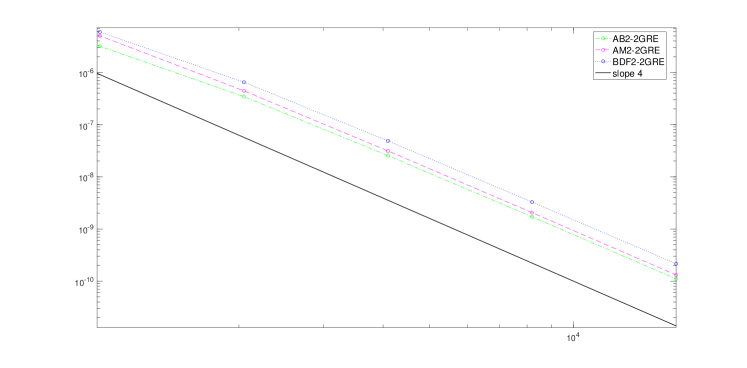
Figure 1: Results for the van der Pol equation for LMM-2GREs, number of grid points versus the global error in maximum norm

Tables 2 and 3, and Figure 2 illustrate the expected $5^{\text{th}}$-order of convergence for all tested LMM-RGREs.

$\text{AB}3$-2GRE	$\text{AM}3$-2GRE	$\text{BDF}3$-2GRE	$\text{AB}2$-3GRE	$\text{AM}2$-3GRE	$\text{BDF}2$-3GRE
5.0121	5.0319	5.2081	4.8145	5.0564	5.1449

Table 2: The estimated order of convergence for the Dahlquist problem for different $5^{\text{th}}$-order LMM-RGREs with $256$ and $512$ grid points

$\text{AB}3$-2GRE	$\text{AM}3$-2GRE	$\text{BDF}3$-2GRE	$\text{AB}2$-3GRE	$\text{AM}2$-3GRE	$\text{BDF}2$-3GRE
4.4933	4.8252	5.4540	6.1243	4.2922	4.0779
5.0397	4.9769	5.4343	5.4060	4.8533	4.7738
5.0747	4.9996	5.2692	5.2996	4.9615	4.9942
4.9983	4.9509	5.2278	5.2431	4.9864	4.9914

Table 3: The estimated order of convergence for the Lotka–Volterra system for different $5^{\text{th}}$-order LMM-RGREs with $256,512,\ldots,4096$ grid points

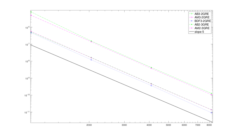
Figure 2: Results for the van der Pol equation for $5^{\text{th}}$-order LMM-RGREs, number of grid points versus the global error in maximum norm

References

- [1] T. Bayleyegn, Á. Havasi, Multiple Richardson Extrapolation Applied to Explicit Runge–Kutta Methods, Advances in High Performance Computing. Springer, 902, 262–270, (2020), http://doi.org/10.1007/978-3-030-55347-0_22
- [2] D. S. Bernstein, Matrix Mathematics, Princeton Univ. Press (2009), https://doi.org/10.1515/9781400833344
- [3] J. C. Butcher, Numerical Methods for Ordinary Differential Equations, 3rd edition, Wiley (2016), https://doi.org/10.1002/9781119121534
- [4] R. D. Falgout, T. A. Manteuffel, B. O’Neill, J. B. Schroder, Multigrid reduction in time with Richardson extrapolation, Electron. Trans. Numer. Anal., 54, 210–233 (2021), https://doi.org/10.1553/etna_vol54s210
- [5] I. Fekete, L. Lóczi, Linear multistep methods and global Richardson extrapolation, Appl. Math. Letters 133 (2022), https://doi.org/10.1016/j.aml.2022.108267
- [6] W. Gautschi, Numerical Analysis, 2nd edition, Birkhäuser (2012), https://doi.org/10.1007/978-0-8176-8259-0
- [7] E. Hairer, S. P. Norsett, G. Wanner, Solving Ordinary Differential Equations I, Nonstiff Problems, 2nd revised edition, Springer-Verlag (1993), https://doi.org/10.1007/978-3-540-78862-1
- [8] Z. Jackiewicz, General Linear Methods for Ordinary Differential Equations, Wiley (2009), https://doi.org/10.1002/9780470522165
- [9] R. J. LeVeque, Finite Difference Methods for Ordinary and Partial Differential Equations: Steady-State and Time-Dependent Problems, SIAM, Philadelphia (2007), https://doi.org/10.1137/1.9780898717839
- [10] A. Ralston, Runge–Kutta methods with minimum error bounds, Math. Comp., 16, 431–437 (1962), https://doi.org/10.1090/S0025-5718-1962-0150954-0
- [11] L. F. Richardson, The approximate arithmetical solution by finite differences of physical problems including differential equations, with an application to the stresses in a masonry dam, Philos. Trans. Roy. Soc. London Ser. A., 210, 307–357 (1911), https://doi.org/10.1098/rsta.1911.0009
- [12] L. F. Richardson, The deferred approach to the limit, Philos. Trans. Roy. Soc. London Ser. A., 226, 299–361 (1927), https://doi.org/10.1098/rsta.1927.0008
- [13] Z. Zlatev, I. Dimov, I. Faragó, Á. Havasi, Richardson Extrapolation: Practical Aspects and Applications, Berlin, Boston: De Gruyter (2017), https://doi.org/10.1515/9783110533002
- [14] Z. Zlatev, I. Dimov, I. Faragó, K. Georgiev, Á. Havasi, Explicit Runge–Kutta Methods Combined with Advanced Versions of the Richardson Extrapolation, Comput. Methods Appl. Math. 20(4) 739–762 (2020), https://doi.org/10.1515/cmam-2019-0016
- [15] Z. Zlatev, I. Dimov, I. Faragó, Á. Havasi, Efficient implementation of advanced Richardson extrapolation in an atmospheric chemical scheme, J. Math. Chem., 60 (1), 219–238 (2022), https://doi.org/10.1007/s10910-021-01300-z