Certification of unbounded randomness without nonlocality

Abstract

Random number generators play an essential role in cryptography and key distribution. It is thus important to verify whether the random numbers generated from these devices are genuine and unpredictable by any adversary. Recently, quantum nonlocality has been identified as a resource that can be utilised to certify randomness. Although these schemes are device-independent and thus highly secure, the observation of quantum nonlocality is extremely difficult from a practical perspective. In this work, we provide a scheme to certify unbounded randomness in a semi-device-independent way based on the maximal violation of Leggett-Garg inequalities. Interestingly, the scheme is independent of the choice of the quantum state, and consequently even "quantum" noise could be utilized to self-test quantum measurements and generate unbounded randomness making the scheme highly efficient for practical purposes.

I Introduction

Random numbers play a crucial role in cryptography and key distribution, serving as a fundamental ingredient for ensuring the security and confidentiality of sensitive information. These classical random number generators are based on the limited knowledge of the physical process that generates these numbers. Consequently, one needs to trust that the knowledge of the process is completely hidden from any adversary who might have access to these devices. The randomness of such numbers is thus certified in a device-dependent way.

Unlike classical physics where in principle events are determined with certainty, quantum theory describes the behavior of particles and systems in terms of probabilities. Further on, the unpredictability of measurement outcomes in quantum theory is intrinsic and not due to ignorance, thus serving as an excellent tool for generating random numbers. In recent times, the concept of quantum non-locality, manifested by the violation of Bell inequalities [1], has emerged as a means to certify randomness in a device-independent (DI) manner [2, 3]. This implies that the assessment of randomness is decoupled from the specific physical characteristics or details of the experimental setup. There are several schemes that utilize quantum nonlocality for DI certification of randomness [4, 5, 6, 7, 8, 9, 10, 11].

However, from a practical perspective, observation of quantum non-locality in a loophole-free way is an extremely difficult task. Most of these experiments are short-ranged and highly sensitive to noise [12, 13, 14, 15]. As a consequence, it is worth exploring scenarios that are noise resistant and easy to implement. In this regard, some physically well-motivated assumptions can be made on the devices which do not compromise much over security but are easier to implement. Such schemes are known as semi-device-independent (SDI). One such assumption is that one of the parties involved in the experiment is fully trusted, that is, the measurements performed by the trusted party are known. Such schemes are considered to be one-sided device-independent (ISDI) [16, 17, 18, 19]. In particular, Ref. [19] proposes a 1SDI scheme to certify the optimal randomness from measurements with arbitrary number outcomes.

In this work, we consider a sequential scenario inspired by Leggett-Garg (LG) inequalities [20] where a single system is measured in a "time-like" separated way. Any violation of LG inequality implies that quantum theory violates the notion of "memoryless" hidden variable models, which as a matter of fact can also be violated in classical physics. For instance, even a classical pre-programmed device can reproduce any observed correlations in the sequential scenario [see below for detailed explanation]. Consequently, an assumption that we impose in this work is that the correlations obtained in the experiment are generated by input-consistent measurements acting on some quantum state, which then allows us to exclude the possibility of classical pre-proggramed devices. Thus, the scheme proposed in this work is semi device-independent. For our purpose, we consider the generalized LG inequality with arbitrary number of inputs [21] and self-test qubit measurements spanning the entire $X-Z$ plane up to the presence of local unitaries. For a note, self-testing of quantum measurements using the LG inequalities for the particular case of four inputs was proposed in [22] and its generalization to arbitrary number of outcomes was proposed in [23] that assumed a particular form of the initial quantum state. Then, we utilise the certified measurements to certify unbounded amount of randomness from the untrusted devices.

A scheme proposed in [8] also utilises sequential measurements for generating unbounded randomness. However, it is based on violation of Bell inequalities which is again difficult to observe. Interestingly, the scheme presented in this work is independent of the initial quantum state and thus even "quantum" noise can be used to generate unbounded randomness. To the best of our knowledge, this is the first scheme that can be used to generate unbounded randomness in a state-independent way. Further on, violation of LG inequalities have been observed in a large number of quantum systems [24, 25, 26, 27, 28], thus making our scheme an excellent candidate for practical random number generators.

II Sequential scenario

The sequential scenario consists of a source and a measurement device with $n-$inputs labeled as $x=1,2,\ldots,n$ and binary outcomes labeled as $a=0,1$. Now in a single run of the experiment, the user provides an arbitrary number of inputs in a sequential manner (one after another) to the device and records their outcomes. From the experiment one can obtain the distribution $\vec{p}_{N}=\{p(a_{1},a_{2},\ldots,a_{N}|x_{1},x_{2},\ldots,x_{N})\}$ where $N$ is the number of consecutive inputs and $p(a_{1},a_{2},\ldots,a_{N}|x_{1},x_{2},\ldots,x_{N})$ signifies the probability of obtaining outcomes $a_{1},a_{2},\ldots,a_{N}$ consequetively when one inputs $x_{1},x_{2},\ldots,x_{N}$ to the device [see Fig. 1].

Using the above set-up Leggett and Garg proposed a test referred to as "Leggett-Garg (LG)" inequality that allows one to exclude macrorealist non-invasive description of quantum theory [for detailed analysis refer to [29]]. The LG inequality is given by

$$\mathcal{L} = \sum_{i=1,\ldots,N-1}C_{x,x+1}-C_{n,1}\leq\beta_{\mathcal{M}}(n)$$ (1)

where the terms $C_{x,y}$ represent the two-time correlation between the inputs $x,y$ and can be obtained via $\vec{p}_{2}$ as

$$C_{x,y}=\sum_{a_{1},a_{2}}(-1)^{a_{1}+a_{2}}p(a_{1},a_{2}|x,y).$$ (2)

The above correlation can be generalized to an arbitrary number of sequential measurements $C_{x_{1},x_{2},\ldots,x_{N}}$ as

$$C_{x_{1},\ldots,x_{N}}=\sum_{a_{1},\ldots,a_{N}}(-1)^{a_{1}+\ldots+a_{N}}p(a_{1},\ldots,a_{N}|x_{1},\ldots,x_{N}).$$ (3)

In the inequality (1), $\beta_{\mathcal{M}}(n)$ denotes the maximum value that one can achieve when the distribution $\vec{p}_{2}$ can be expressed via "time-local" or "memory-less" hidden variable models given as

$$p(a_{1},a_{2}|x,y)=\sum_{\lambda}p(a_{1}|x,\lambda)p(a_{2}|y,\lambda)p(\lambda).$$ (4)

with the value $\beta_{\mathcal{M}}(n)=n-2$.

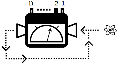
Figure 1: The sequential scenario. The source sends a single system into the measurement device with $n$ inputs labeled as $x=1,2,\ldots,n$ and binary outcomes labeled as $a=0,1$. The quantum state is measured in sequential way to obtain the probability distribution $\vec{p}_{N}$.

Let us now restrict ourselves to quantum theory where each input $i$ corresponds to a fixed measurement $A_{i}=\{\mathbbm{M}_{i,0},\mathbbm{M}_{i,1}\}$ where $\mathbbm{M}_{i,j}$ represent measurement elements that are Hermitian and $\sum_{j}\mathbbm{M}_{i,j}=\mathbbm{1}$. The measurement elements in general are not projective. Consequently, the corresponding probability $p(a_{1},a_{2}|A_{1},A_{2})$ is given by

$$p(a_{1},a_{2}|A_{1},A_{2})=\mathrm{Tr}\left(\sqrt{\mathbbm{M}_{1,a_{1}}}\ U_{a_{1}}^{\dagger}\mathbbm{M}_{2,a_{1}}U_{a_{1}}\sqrt{\mathbbm{M}_{1,a_{1}}}\ \rho_{A}\right)$$ (5)

where $U_{a_{1}}$ is some unitary dependent on the outcome $a_{1}$ and $\rho_{A}$ is some quantum state. The above rule to compute probability can be straightaway generalised to an arbitrary number of sequential measurements.

Let us now consider that the measurements $A_{i}$ corresponding to each input $i$ are projective. As pointed out by Fritz in [30] for projective measurements, the correlation $C_{x,y}$ in quantum theory is expressed as $C_{x,y}=1/2\left\langle\{\mathcal{A}_{x},\mathcal{A}_{y}\}\right\rangle$ where $\mathcal{A}_{x}$ denotes the observable corresponding to the $x-th$ measurement represented in terms of the measurement elements $\Pi_{x,j}\ (j=0,1)$ as

$$\mathcal{A}_{x}=\Pi_{x,0}-\Pi_{x,1}.$$ (6)

It is simple to observe that $\mathcal{A}_{x}^{2}=\mathbbm{1}$. Consequently, $p(a_{1},a_{2},\ldots,a_{N}|x_{1},x_{2},\ldots,x_{N})$ is expressed for projective measurements as

$$p(a_{1},a_{2},\ldots,a_{N}|x_{1},x_{2},\ldots,x_{N})=\qquad\qquad\qquad\qquad$$

$$\mathrm{Tr}\left(\Pi_{x_{1},a_{1}}\ldots\Pi_{x_{N-1},a_{N-1}}\Pi_{x_{N},a_{N}}\Pi_{x_{N-1},a_{N-1}}\ldots\Pi_{x_{1},a_{1}}\rho\right)$$

Thus, for projective measurements in quantum theory the witness $\mathcal{L}$ from (1) is given by

$$\mathcal{L} = \frac{1}{2}\sum_{x=1}^{N-1}\left\langle\{\mathcal{A}_{x},\mathcal{A}_{x+1}\}\right\rangle-\frac{1}{2}\left\langle\{\mathcal{A}_{n},\mathcal{A}_{1}\}\right\rangle.$$ (8)

Consider now the following observables

$$\tilde{\mathcal{A}}_{x}=\cos{\frac{\pi(x-1)}{n}}\sigma_{z}+\sin{\frac{\pi(x-1)}{n}}\sigma_{x}$$ (9)

where $\sigma_{z},\sigma_{x}$ are the Pauli $z,x$ matrices. Now, a simple computation of the functional (8) using the observables (9) yields the value $\beta_{Q}(n)=n\cos{\frac{\pi}{n}}$ which is strictly greater than $\beta_{\mathcal{M}}(n)$. We will show later that $\beta_{Q}(n)$ is in fact the maximum value of $\mathcal{L}$ attainable using quantum theory when restricting to projective measurements.

Before proceeding, let us recall an important constraint that is imposed on the distribution $\vec{p}_{N}$ known as "no-signalling in time" [29] conditions given by

$$\sum_{\begin{subarray}{c}i=1\\ i\neq k\end{subarray}}^{N}\sum_{a_{i}=0,1}p(a_{1},a_{2},\ldots,a_{N}|x_{1},x_{2},\ldots,x_{N})=p(a_{k}|x_{k})$$ (10)

for any $y_{1},\ldots,y_{N}$. Before proceeding to the main results, let us now comment on whether the above-described sequential scenario can be utilised for device-independent quantum information or not.

III Device-independent viewpoint on sequential scenarios

Quantum protocols where one does not require to trust the devices are termed device-independent. These are particularly useful in quantum cryptography and key distribution where an adversary might have access to the devices. Recently, the task of DI certification of quantum states and measurements has gained a lot of interest as states and measurements inside the device can be characterized without any knowledge about the inner workings of the device. Most of these certification schemes are based on violation of a Bell inequality.

Let us now consider the sequential scenario described above [sec II]. As all the operations of the device occur locally where the device might have access to the previous inputs and outputs, even a classical pre-programmed device can simulate any distribution $\vec{p}_{N}$ obtained in the sequential scenario and still satisfy the "no-signalling" in time constraint [Eq. (10)]. For instance, the device might already have a list of instructions conditioned on the previous input and output in a stochastic way and build up the observed statistics. This possibility can never be excluded unless one finds some physical constraint such that the device does not store the information of the previous input and output. In the Bell scenario, this possibility is excluded due to the space-like separation that does not allow one side to gain information about the other side. This has also been noted in several certification schemes based on sequential sequential scenarios. For instance, in [23] a major assumption was that the correlations are generated from the measurements acting on a known quantum state. Here we do not assume any form of the quantum state.

IV Self-testing quantum measurements in a state-independent way

Self-testing is a method of DI certification where one can characterize the quantum states and measurements inside an untrusted device up to some degree of freedom under which the observed probabilities remain invariant. In this section, we self-test any qubit measurement in the $X-Z$ plane. To begin with, let us clearly state the major assumption that is imposed in the sequential scenario for obtaining the self-testing result.

Assumption 1.

The correlations $\vec{p}_{N}$ obtained in the sequential scenario [see Fig. 1] are generated by measurements that are consistent for a particular input.

The consistency of measurements for a particular input ensures that they are independent of any previous input-output. This allows us to consider that $A_{i}^{\prime}s$ are POVM’s as discussed in sec II. Let us now revisit the previous experiment [see Fig. 1] in which a user sequentially measures a quantum state $\rho_{A}$ sent by the source and observes the correlations $\vec{p}_{N}$. Consider now a reference experiment that reproduces the same statistics as the actual experiment but involves the states $\tilde{\rho}_{A}$ and observables represented by $\tilde{\mathcal{A}}_{i}$. The observables $\mathcal{A}_{i}$ are self-tested from $\vec{p}_{N}$ if there exists a unitary $\mathcal{U}:\mathcal{H}_{A}\to\mathcal{H}_{A^{\prime}}\otimes\mathcal{H}_{A^{\prime\prime}}$ such that

$$\mathcal{U}\mathcal{A}_{i}\mathcal{U}^{\dagger}=\tilde{\mathcal{A}}_{i}\otimes\mathbbm{1}_{A^{\prime\prime}},$$ (11)

where $\mathcal{H}_{A^{\prime\prime}}$ denotes the junk Hilbert space and $\mathbbm{1}_{A^{\prime\prime}}$ denotes the identity acting on $\mathcal{H}_{A^{\prime\prime}}$. The self-testing result presented in this work is state-independent and consequently no state can be certified using our scheme. Before proceeding, let us recall that the observables can be certified on the support of the quantum state. Thus without loss of generality throughout the manuscript, we will assume that the quantum state $\rho_{A}$ is full-rank.

Let us now restrict ourselves to the probability distribution $\vec{p}_{2}$. Inspired by [23], we impose the following condition on $\vec{p}_{2}$.

Definition 1 (Zeno conditions).

If the same measurement $A_{i}$ for any $i$ is performed sequentially, then for both measurement events the same outcome occurs with certainty. This implies that the distribution $\vec{p}_{2}$ is constrained as

$$p(a,b|A_{i},A_{i})=\delta_{a,b}p(a|A_{i})\qquad\forall i.$$ (12)

Using assumption 1, we show in fact 2 in the appendix, that the condition (12) implies that the measurements $A_{i}$ are projective. This allows us to consider the Leggett-Garg functional (8). Let us show that $\beta_{Q}(n)$ is the maximal quantum value of $\mathcal{L}$ (8). For this purpose, we consider the LG operator $\hat{\mathcal{L}}$ given by

$$\hat{\mathcal{L}} = \frac{1}{2}\sum_{x=1}^{N-1}\{\mathcal{A}_{x},\mathcal{A}_{x+1}\}-\frac{1}{2}\{\mathcal{A}_{n},\mathcal{A}_{1}\}.$$ (13)

Consider now the following operators $P_{i}$ for $i=1,\ldots,n-2$ given by

$$P_{i}=\mathcal{A}_{i}-\alpha_{i}\mathcal{A}_{i+1}+\beta_{i}\mathcal{A}_{n}$$ (14)

where

$$\alpha_{i}=\frac{\sin\left(\frac{\pi i}{n}\right)}{\sin\left(\frac{\pi(i+1)}{n}\right)},\qquad\beta_{i}=\frac{\sin\left(\frac{\pi}{n}\right)}{\sin\left(\frac{\pi(i+1)}{n}\right)}.$$ (15)

After some simplification, one can observe that

$$\sum_{i=1}^{N-2}\frac{1}{2\alpha_{i}}P_{i}^{\dagger}P_{i}=\frac{1}{2}\sum_{i=1}^{n-2}\left(\frac{1}{\alpha_{i}}+\alpha_{i}+\frac{\beta_{i}^{2}}{\alpha_{i}}\right)\mathbbm{1}-\hat{\mathcal{L}}$$ (16)

where we used the fact that $\mathcal{A}_{i}^{2}=\mathbbm{1}$. Notice that the term on the left-hand side of the above formula is positive which allows us to conclude that

$$\hat{\mathcal{L}}\leq\frac{1}{2}\sum_{i=1}^{n-2}\left(\frac{1}{\alpha_{i}}+\alpha_{i}+\frac{\beta_{i}^{2}}{\alpha_{i}}\right)\mathbbm{1}$$ (17)

In Fact 2 in the appendix, we show that

$$\sum_{i=1}^{n-2}\left(\frac{1}{\alpha_{i}}+\alpha_{i}+\frac{\beta_{i}^{2}}{\alpha_{i}}\right)=2\beta_{Q}(n)$$ (18)

which allows us to infer from (16) that

$$\hat{\mathcal{L}}\leq\beta_{Q}(n)\mathbbm{1}.$$ (19)

Consequently, $\beta_{Q}(n)$ is the maximal quantum value of $\mathcal{L}$ (8).

Now, let us assume that one observes the value $\beta_{Q}(n)$ of the LG functional $\mathcal{L}$ (8). Thus from the decomposition (16), we have that

$$\mathrm{Tr}(P_{i}^{\dagger}P_{i}\rho_{A})=0,\qquad i=1,\ldots,n-2.$$ (20)

The above relation (20) will be particularly useful for self-testing as stated below.

Theorem 2.

Assume that the Zeno conditions (12) are satisfied and the LG inequality (1) is maximally violated by some state $\rho_{A}$ and observables $\mathcal{A}_{i}\ (i=1,\ldots,n)$. Then, the following statements hold true:

1. The observables $\mathcal{A}_{i}$ act on the Hilbert space $\mathcal{H}_{A}=(\mathbbm{C}^{2})_{A^{\prime}}\otimes\mathcal{H}_{A^{\prime\prime}}$ for some auxiliary Hilbert space $\mathcal{H}_{A^{\prime\prime}}$.

2.    There exist unitary transformations, $\mathcal{U}:\mathcal{H}_{A}\rightarrow\mathcal{H}_{A}$, such that

$$\mathcal{U}\mathcal{A}_{i}\mathcal{U}^{\dagger}=\tilde{\mathcal{A}}_{i}\otimes\mathbbm{1}_{A^{\prime\prime}}.$$ (21)

where the observables $\tilde{\mathcal{A}}_{i}$ are listed in Eq. (9).

Proof.

Let us begin by considering the relation (20) which can be rewritten as $||P_{i}\sqrt{\rho_{A}}||=0$ for $i=1,\ldots,n-2$ and thus we obtain that $P_{i}\sqrt{\rho_{A}}=0$. As $\rho_{A}$ is full-rank, we simply arrive at the condition $P_{i}=0$ which can be expanded using (14) to obtain

$$\mathcal{A}_{i}=\alpha_{i}\mathcal{A}_{i+1}-\beta_{i}\mathcal{A}_{n}\qquad i=1,\ldots,n-2.$$ (22)

Let us now consider $i=1$ in the above formula (22) and substitute $\alpha_{1},\beta_{1}$ from Eq. (15) to arrive at

$$\mathcal{A}_{1}=\frac{1}{2\cos\left(\frac{\pi}{n}\right)}(\mathcal{A}_{2}-\mathcal{A}_{n}).$$ (23)

Again using the fact that $\mathcal{A}_{i}^{2}=\mathbbm{1}$, allows us to conclude from the above formula (23)

$$\frac{1}{4\cos^{2}\left(\frac{\pi}{n}\right)}(\mathcal{A}_{2}-\mathcal{A}_{n})^{2}=\mathbbm{1}$$ (24)

which on further expansion gives us

$$\{\mathcal{A}_{2},\mathcal{A}_{n}\}=2\left[1-2\cos^{2}\left(\frac{\pi}{n}\right)\right]\mathbbm{1}.$$ (25)

Let us now show that the observables $\mathcal{A}_{i}$ for any $i$ are traceless. For this purpose, we consider the above formula (25) and multiply it with $\mathcal{A}_{2}$ and then take the trace to obtain

$$\mathrm{Tr}(\mathcal{A}_{n})=\left[1-2\cos^{2}\left(\frac{\pi}{n}\right)\right]\mathrm{Tr}(\mathcal{A}_{2}).$$ (26)

Again, we consider Eq. (25) and multiply it with $\mathcal{A}_{n}$ and then take the trace to obtain

$$\mathrm{Tr}(\mathcal{A}_{2})=\left[1-2\cos^{2}\left(\frac{\pi}{n}\right)\right]\mathrm{Tr}(\mathcal{A}_{n}).$$ (27)

It is straightforward from Eqs. (26) and (27), that $\mathrm{Tr}(\mathcal{A}_{2})=\mathrm{Tr}(\mathcal{A}_{n})=0$ for any $n\geq 3$. Further on, taking trace on both sides of Eq. (22) for any $i$, allows us to conclude that $\mathrm{Tr}(\mathcal{A}_{i})=0$. Thus, the number of eigenvalues $(1,-1)$ of the observables $\mathcal{A}_{i}$ are equal. Consequently, the observables $\mathcal{A}_{i}$ act on $\mathbbm{C}^{2}\otimes\mathcal{H}_{A^{\prime\prime}}$.

Let us now characterize the observables $\mathcal{A}_{i}$. For this purpose, we observe from (25) that

$$\frac{1}{4\sin^{2}\left(\frac{\pi}{n}\right)}(\mathcal{A}_{2}+\mathcal{A}_{n})^{2}=\mathbbm{1}.$$ (28)

Let us further notice that $\{\mathcal{A}_{2}-\mathcal{A}_{n},\mathcal{A}_{2}+\mathcal{A}_{n}\}=0$ which can rewritten as

$$\left\{\frac{1}{2\cos\left(\frac{\pi}{n}\right)}(\mathcal{A}_{2}-\mathcal{A}_{n}),\frac{1}{2\sin\left(\frac{\pi}{n}\right)}(\mathcal{A}_{2}-\mathcal{A}_{n})\right\}=0.$$ (29)

As proven in [31], if two matrices $A,B$ anti-commute and $A^{2}=B^{2}=\mathbbm{1}$, then there exist a unitary transformation $\mathcal{U}$ such that $\mathcal{U}A\mathcal{U}^{\dagger}=\sigma_{z}\otimes\mathbbm{1}$ and $\mathcal{U}B\mathcal{U}^{\dagger}=\sigma_{x}\otimes\mathbbm{1}$. Thus, from Eqs. (23), (28) and (29) we obtain that

$$\mathcal{A}^{\prime}_{2}-\mathcal{A}^{\prime}_{n} = 2\cos\left(\frac{\pi}{n}\right)\sigma_{z}\otimes\mathbbm{1},$$

$$\mathcal{A}^{\prime}_{2}+\mathcal{A}^{\prime}_{n} = 2\sin\left(\frac{\pi}{n}\right)\sigma_{x}\otimes\mathbbm{1}$$ (30)

where $\mathcal{A}^{\prime}_{i}=\mathcal{U}\mathcal{A}_{i}\mathcal{U}^{\dagger}$. Thus, we obtain from Eqs. (23) and (IV) that

$$\mathcal{A}^{\prime}_{1} = \sigma_{z}\otimes\mathbbm{1}$$

$$\mathcal{A}^{\prime}_{2} = \left(\cos{\frac{\pi}{n}}\sigma_{z}+\sin{\frac{\pi}{n}}\sigma_{x}\right)\otimes\mathbbm{1}$$

$$\mathcal{A}^{\prime}_{n} = \left(-\cos{\frac{\pi}{n}}\sigma_{z}+\sin{\frac{\pi}{n}}\sigma_{x}\right)\otimes\mathbbm{1}.$$ (31)

Now, let us consider the condition (22) for $i=2$ and apply $\mathcal{U}$ on both the sides to obtain

$$\mathcal{A}^{\prime}_{2}=\alpha_{2}\mathcal{A}^{\prime}_{3}-\beta_{2}\mathcal{A}^{\prime}_{n}.$$ (32)

Now, substituting $\alpha_{2},\beta_{2}$ from Eq. (15) and $\mathcal{A}^{\prime}_{2},\mathcal{A}^{\prime}_{n}$ from (IV) and then after some trigonometric simplification, we obtain

$$\mathcal{A}^{\prime}_{3}=\left(\cos{\frac{2\pi}{n}}\sigma_{z}+\sin{\frac{2\pi}{n}}\sigma_{x}\right)\otimes\mathbbm{1}.$$ (33)

Continuing in a similar fashion for all $i^{\prime}s$ allows us to conclude that for $i=1,2,\ldots,n$

$$\mathcal{A}_{i}^{\prime}=\left(\cos{\frac{\pi(i-1)}{n}}\sigma_{z}+\sin{\frac{\pi(i-1)}{n}}\sigma_{x}\right)\otimes\mathbbm{1}.$$ (34)

This completes the proof. ∎

Interestingly, the above self-testing result is valid for any quantum state. Let us now utilize the above self-testing result to certify randomness generated from the untrusted measurements.

V State-independent unbounded randomness expansion

Here we certify unbounded randomness from the untrusted measurement in the sequential scenario. For this purpose, we first consider assumption 1 along with the Zeno conditions (12) which ensures that the measurements are projective. Let us now restrict to even $n$ and consider the correlation $C_{i,i+n/2,i,i+n/2,\ldots}$ for any $i$ such that $(i=2,\ldots,\frac{n}{2})$ corresponding to the distribution when the observables $\mathcal{A}_{i},\mathcal{A}_{i+n/2}$ are sequentially measured. In terms of probabilities, the correlation $C_{i,i+n/2,i,i+n/2,\ldots}$ is expressed in Eq. (3). Consequently, we modify the LG inequality as

$$\mathcal{R}_{i}=\mathcal{L}-|C_{i,i+n/2,i,i+n/2,\ldots}|\quad i=2,\ldots,\frac{n}{2}.$$ (35)

Notice that using the observables listed in (9), one can attain the value $\beta_{Q}(n)=n\cos(\frac{\pi}{n})$ of $\mathcal{R}_{i}$ for any $i$. As $\mathcal{R}_{i}\leq\mathcal{L}$, it is thus clear that the maximum quantum value of $\mathcal{R}_{i}$ is the same as $\mathcal{L}$. Now, if one observes the maximal quantum value $\beta_{Q}(n)$ of $\mathcal{R}_{i}$, then $|C_{i,i+n/2,i,i+n/2,\ldots}|=0$ and $\mathcal{L}=\beta_{Q}(n)$. Thus, from theorem 2, we can conclude that the observables $\mathcal{A}_{i}$ are certified as in (21).

Now, let us compute the guessing probability of an adversary Eve who might have access to the user’s quantum state. The joint state of Eve and the user is denoted as $\rho_{AE}$ such that $\rho_{A}=\mathrm{Tr}_{E}(\rho_{AE})$. As Eve’s dimension is unrestricted, without loss to generality we assume that $\rho_{AE}$ is pure and denote it further as $\psi_{AE}$. To guess the user’s outcome, she could then perform some measurement $\mathbbm{Z}=\{Z_{e}\}$, where $e$ denotes the outcome of Eve, on her part of the joint quantum state $\psi_{AE}$. The probability of Eve obtaining an outcome $e=a$ given the user’s outcome $a$ is denoted as $p(e=a|a,\mathbbm{Z})$. Since Eve does not have access to the outcome $a$, the guessing probability of Eve is averaged over the outcomes of the user giving us the following expression

$$p_{guess}(E|S)=\max_{\mathbbm{Z}}\sum_{a}p(a)p(e=a|a,\mathbbm{Z})$$ (36)

where $S$ denotes the system of the user and $a\equiv\{a_{1},a_{2},\ldots,a_{N}\}$. Now, expressing (36) in quantum theory, we obtain that

$$p_{guess}(E|S)=\max_{\mathbbm{Z}}\sum_{a}\mathrm{Tr}\left(\Pi_{x_{1},a_{1}}\Pi_{x^{\prime},a^{\prime}}\Pi_{x_{1},a_{1}}\otimes Z_{a}\psi_{AE}\right)$$ (37)

where

$$\Pi_{x^{\prime},a^{\prime}}=\Pi_{x_{2},a_{2}}\ldots\Pi_{x_{N-1},a_{N-1}}\Pi_{x_{N},a_{N}}\Pi_{x_{N-1},a_{N-1}}\ldots\Pi_{x_{2},a_{2}}.$$ (38)

The projectors $\Pi_{x_{i},a_{i}}$ are certified from Eq. (21) as $\Pi_{x_{i},a_{i}}=\mathcal{U}^{\dagger}\left(|e_{x_{i},a_{i}}\rangle\!\!\langle e_{x_{i},a_{i}}|\otimes\mathbbm{1}\right)\mathcal{U}$, where $|e_{x_{i},a_{i}}\rangle$ are the eigenstates of $\tilde{\mathcal{A}}_{x_{i}}$ [see Eq. (9)]. Thus, the guessing probability from Eq. (V) can be simplified to

$$p_{guess}(E|S)=\qquad\qquad\qquad\qquad\qquad\qquad\qquad$$

$$\max_{\mathbbm{Z}}\sum_{a}\mathcal{N}_{a}\ \mathrm{Tr}\left(|e_{x_{1},a_{i}}\rangle\!\!\langle e_{x_{1},a_{i}}|\otimes\mathbbm{1}_{A^{\prime\prime}}\otimes Z_{a}\psi_{AE}\right)$$ (39)

where

$$\mathcal{N}_{a}=\prod_{l=1,N-1}|\langle{e_{x_{l},a_{i}}}|e_{x_{l+1},a_{i}}\rangle|^{2}.$$ (40)

Now, choosing $x_{1}=2,x_{2}=2+n/2,x_{3}=2,x_{4}=2+n/2\ldots$ we obtain that $\mathcal{N}_{a}=\frac{1}{2^{N-1}}$ for any $a$. Thus, the expression (V) is further simplified to

$$p_{guess}(E|S)=\qquad\qquad\qquad\qquad\qquad\qquad\qquad$$

$$\frac{1}{2^{N-1}}\max_{\mathbbm{Z}}\sum_{a}\ \mathrm{Tr}\left(|e_{x_{1},a_{i}}\rangle\!\!\langle e_{x_{1},a_{i}}|\otimes\mathbbm{1}_{A^{\prime\prime}}\otimes Z_{a}\psi_{AE}\right)$$ (41)

As the observable $\mathcal{A}_{x_{1}}$ acts on $\mathbbm{C}^{2}\otimes\mathcal{H}_{A^{\prime\prime}}$, we express the state $|\psi_{AE}\rangle$ as

$$|\psi_{AE}\rangle=\sum_{i=0,1}\lambda_{a_{i}}|e_{x_{1},a_{i}}\rangle_{A^{\prime}}|f_{i}\rangle_{A^{\prime\prime}E}.$$ (42)

such that $\sum_{i=0,1}\lambda_{a_{i}}^{2}=1$ and the states $|f_{i}\rangle_{A^{\prime\prime}E}$ are in general not othogonal. Plugging the above state Eq. (42) into Eq. (V) gives us

$$p_{guess}(E|S)=\frac{1}{2^{N-1}}\max_{\mathbbm{Z}}\sum_{a}\lambda_{a_{i}}^{2}\ \langle f_{i}|\mathbbm{1}_{A^{\prime\prime}}\otimes Z_{a}|f_{i}\rangle.$$ (43)

Using the fact that $\sum_{a}Z_{a}=\mathbbm{1}$, we finally obtain that

$$p_{guess}(E|S)=\frac{1}{2^{N-1}}.$$ (44)

The amount of randomness that can be extracted is quantified by the min-entropy of Eve’s guessing probability [2]. Consequently, we obtain $N-1$ bits of randomness from $N-$sequential measurements. In principle, $N$ can be arbitrarily large and thus we can obtain an unbounded amount of randomness. Let us stress here that one can also obtain unbounded randomness when $n$ is odd. However, the amount of randomness obtained with $N-$sequential measurements is lower when $n$ is odd than even.

VI Conclusions

In this work, we first provided a semi-device independent self-testing of qubit measurements spanning the $X-Z$ plane independent of the initial quantum state that is fed into the device under the assumption that the correlations are generated by input-consistent measurements acting on a quantum state. Let us again stress here that such an assumption is natural in space-like separated scenarios but is an ad-hoc assumption for the time-like separated scenario considered in this work. We then utilised the certified measurements to generate unbounded amount of randomness from the untrusted devices in a state-independent way.

Several follow-up problems arise from our work. The assumption of measurements being consistent is strict and thus it would be highly desirable to extend the framework of LG inequalities to case when the measurements might depend on previous input-output. Another interesting problem would be to find the robustness of our protocol towards experimental imperfections. Further on, it would be highly desirable to generalise the above scheme to arbitrary number of outcomes. Consequently, one could generate an arbitrary amount of randomness from a single measurement in a state-independent way. It would also be highly desirable if one can self-test any qubit measurement in a single experiment using the above scheme thus providing a state-independent certification of tomographically complete set of measurements.

VII Acknowledgements

We would like to thank Stefano Pironio for useful insights. This project was funded within the QuantERA II Programme (VERIqTAS project) that has received funding from the European Union’s Horizon 2020 research and innovation programme under Grant Agreement No 101017733.

Appendix A Projectivity of quantum measurements

Fact 1.

Assume that in the sequential scenario depicted in Fig. 1, the correlations $\vec{p}_{2}$ are generated via input-consistent measurements $A_{i}$ acting on some quantum state $\rho_{A}$ [see assumption 1]. Then the Zeno conditions (12) implies that the measurements $A_{i}$ are projective.

Proof.

To begin with, let us expand the condition (12) for $i=1$ using the rule (5) to obtain the following expression

$$\mathrm{Tr}\left(\sqrt{\mathbbm{M}_{a}}\ U_{a}^{\dagger}\mathbbm{M}_{b}U_{a}\sqrt{\mathbbm{M}_{a}}\ \rho_{A}\right)=\delta_{a,b}\mathrm{Tr}\left(\mathbbm{M}_{a}\ \rho_{A}\right)$$ (45)

where for simplicity we dropped the index $i=1$. Let us consider the case when $a\neq b$ in the above expression to obtain the following condition

$$\mathrm{Tr}\left(\sqrt{\mathbbm{M}_{a}}\ U_{a}^{\dagger}\mathbbm{M}_{b}U_{a}\sqrt{\mathbbm{M}_{a}}\ \rho_{A}\right)=\qquad$$

$$||\sqrt{\mathbbm{M}_{b}}U_{a}\sqrt{\mathbbm{M}_{a}}\ \sqrt{\rho_{A}}||=0.$$ (46)

It is straightforward to conclude from the above expression that

$$\sqrt{\mathbbm{M}_{b}}U_{a}\sqrt{\mathbbm{M}_{a}}\ \sqrt{\rho_{A}}=0$$ (47)

which on utilising the fact that $\rho_{A}$ is full-rank and thus invertible, we obtain

$$\sqrt{\mathbbm{M}_{b}}U_{a}\sqrt{\mathbbm{M}_{a}}=0.$$ (48)

Now multiplying $\sqrt{\mathbbm{M}_{b}}$ from left-hand side and $\sqrt{\mathbbm{M}_{a}}$ from right-hand side and using the fact that $\sum_{a}\mathbbm{M}_{a}=\mathbbm{1}$, we obtain that

$$U_{a}\mathbbm{M}_{a}=\mathbbm{M}_{a}U_{a}\mathbbm{M}_{a},\qquad a=0,1.$$ (49)

Let us now expand $\mathbbm{M}_{a}$ using its eigendecomposition as

$$\mathbbm{M}_{a}=\sum_{k}\lambda_{k,a}|e_{k,a}\rangle\!\!\langle e_{k,a}|$$ (50)

where $0\leq\lambda_{k,j}\leq 1$ and $\{|e_{k,a}\rangle\}_{k}$ are orthonormal set of vectors for any $a$. Let us also observe that $U_{a}\mathbbm{M}_{a}=\sum_{k}\lambda_{k,a}|f_{k,a}\rangle\!\langle e_{k,a}|$ where $|f_{k,a}\rangle=U_{a}|e_{k,a}\rangle$. Consequently, we obtain from Eq. (49) that

$$\sum_{k}\lambda_{k,a}\ |f_{k,a}\rangle\!\langle e_{k,a}|=\sum_{l,k}\lambda_{l,a}\lambda_{k,a}\ |e_{l,a}\rangle\!\langle e_{l,a}|f_{k,a}\rangle\!\langle e_{k,a}|.$$ (51)

Sandwiching the above expression with $\langle e_{l,a}|..|e_{k,a}\rangle$ gives us

$$\lambda_{k,a}\ \langle e_{l,a}|f_{k,a}\rangle=\lambda_{l,a}\lambda_{k,a}\ \langle e_{l,a}|f_{k,a}\rangle\qquad\forall l,k.$$ (52)

There exist atleast one $k$ for each $l$ such that $\langle e_{l,a}|f_{k,a}\rangle\neq 0$ or else the condition Eq. (51) can not be satisfied. Thus, we obtain from Eq. (52) that $\lambda_{l,a}=1$ for all $l,a$. Thus, the measurement $\mathbbm{M}_{a}$ from Eq. (50) is projective. ∎

Appendix B Some mathematical fact

Fact 2.

If $\alpha_{i}=\frac{\sin\left(\frac{\pi i}{n}\right)}{\sin\left(\frac{\pi(i+1)}{n}\right)}$ and $\beta_{i}=\frac{\sin\left(\frac{\pi}{n}\right)}{\sin\left(\frac{\pi(i+1)}{n}\right)}$, then

$$\sum_{i=1}^{n-2}\left(\frac{1}{\alpha_{i}}+\alpha_{i}+\frac{\beta_{i}^{2}}{\alpha_{i}}\right)=2n\cos\left(\frac{\pi}{n}\right).$$ (53)

Proof.

Let us first expand the term $t_{i}=\frac{1}{\alpha_{i}}+\alpha_{i}+\frac{\beta_{i}^{2}}{\alpha_{i}}$ for any $i$,

$$t_{i}=\frac{\sin\left(\frac{\pi(i+1)}{n}\right)}{\sin\left(\frac{\pi i}{n}\right)}+\frac{\sin\left(\frac{\pi i}{n}\right)}{\sin\left(\frac{\pi(i+1)}{n}\right)}+\frac{\sin^{2}\left(\frac{\pi}{n}\right)}{\sin\left(\frac{\pi(i+1)}{n}\right)\sin\left(\frac{\pi i}{n}\right)}.$$ (54)

Using the identity $\sin(a+b)=\sin(a)\cos(b)+\sin(b)\cos(a)$, we obtain from Eq. (54) that

$$t_{i}=2\cos\left(\frac{\pi}{n}\right)+\sin\left(\frac{\pi}{n}\right)\left[\cot\left(\frac{\pi i}{n}\right)-\cot\left(\frac{\pi(i+1)}{n}\right)\right]$$

$$+\frac{\sin^{2}\left(\frac{\pi}{n}\right)}{\sin\left(\frac{\pi(i+1)}{n}\right)\sin\left(\frac{\pi i}{n}\right)}.\qquad$$ (55)

Now, expressing

$$\sin\left(\frac{\pi}{n}\right)=\sin\left(\frac{\pi(i+1)}{n}-\frac{\pi i}{n}\right)$$ (56)

and again using the identity $\sin(a+b)=\sin(a)\cos(b)+\sin(b)\cos(a)$, we obtain from Eq. (2)

$$t_{i}=2\cos\left(\frac{\pi}{n}\right)+2\sin\left(\frac{\pi}{n}\right)\left[\cot\left(\frac{\pi i}{n}\right)-\cot\left(\frac{\pi(i+1)}{n}\right)\right]$$ (57)

Now, summing $t_{i}$ over $i$ gives us

$$\sum_{i=1}^{n-2}t_{i} = 2(n-2)\cos\left(\frac{\pi}{n}\right)+4\sin\left(\frac{\pi}{n}\right)\cot\left(\frac{\pi}{n}\right)$$ (58)

$$= 2n\cos\left(\frac{\pi}{n}\right).$$

This completes the proof. ∎

References

• Bell [1964] J.Β S.Β Bell,Β On the einstein podolsky rosen paradox,Β Physics Physique FizikaΒ 1,Β 195 (1964).
• PironioΒ etΒ al. [2010] S.Β Pironio, A.Β AcΓ­n, S.Β Massar, A.Β B.Β deΒ la Giroday, D.Β N.Β Matsukevich, P.Β Maunz, S.Β Olmschenk, D.Β Hayes, L.Β Luo, T.Β A.Β Manning,Β andΒ C.Β Monroe,Β Random numbers certified by bell’s theorem,Β NatureΒ 464,Β 1021 (2010).
• AcΓ­nΒ andΒ Masanes [2016] A.Β AcΓ­nΒ andΒ L.Β Masanes,Β Certified randomness in quantum physics,Β NatureΒ 540,Β 213 (2016).
• AcΓ­nΒ etΒ al. [2016] A.Β AcΓ­n, S.Β Pironio, T.Β VΓ©rtesi,Β andΒ P.Β Wittek,Β Optimal randomness certification from one entangled bit,Β Phys. Rev. AΒ 93,Β 040102 (2016).
• AcΓ­nΒ etΒ al. [2012] A.Β AcΓ­n, S.Β Massar,Β andΒ S.Β Pironio,Β Randomness versus nonlocality and entanglement,Β Phys. Rev. Lett.Β 108,Β 100402 (2012).
• WoodheadΒ etΒ al. [2020] E.Β Woodhead, J.Β Kaniewski, B.Β Bourdoncle, A.Β Salavrakos, J.Β Bowles, A.Β AcΓ­n,Β andΒ R.Β Augusiak,Β Maximal randomness from partially entangled states,Β Phys. Rev. ResearchΒ 2,Β 042028 (2020).
• Ε upiΔ‡Β etΒ al. [2016] I.Β Ε upiΔ‡, R.Β Augusiak, A.Β Salavrakos,Β andΒ A.Β AcΓ­n,Β Self-testing protocols based on the chained bell inequalities,Β New Journal of PhysicsΒ 18,Β 035013 (2016).
• CurchodΒ etΒ al. [2017] F.Β J.Β Curchod, M.Β Johansson, R.Β Augusiak, M.Β J.Β Hoban, P.Β Wittek,Β andΒ A.Β AcΓ­n,Β Unbounded randomness certification using sequences of measurements,Β Phys. Rev. AΒ 95,Β 020102 (2017).
• SarkarΒ etΒ al. [2021] S.Β Sarkar, D.Β Saha, J.Β Kaniewski,Β andΒ R.Β Augusiak,Β npj Quantum InformationΒ 7,Β 151 (2021).
• BorkaΕ‚aΒ etΒ al. [2022] J.Β J.Β BorkaΕ‚a, C.Β Jebarathinam, S.Β Sarkar,Β andΒ R.Β Augusiak,Β Device-independent certification of maximal randomness from pure entangled two-qutrit states using non-projective measurements,Β EntropyΒ 24,Β 10.3390/e24030350 (2022).
• TavakoliΒ etΒ al. [2021] A.Β Tavakoli, M.Β Farkas, D.Β Rosset, J.-D.Β Bancal,Β andΒ J.Β Kaniewski,Β Mutually unbiased bases and symmetric informationally complete measurements in bell experiments,Β Science AdvancesΒ 7,Β eabc3847 (2021).
• AspectΒ etΒ al. [1982] A.Β Aspect, J.Β Dalibard,Β andΒ G.Β Roger,Β Experimental test of bell’s inequalities using time-varying analyzers,Β Phys. Rev. Lett.Β 49,Β 1804 (1982).
• AspectΒ etΒ al. [1981] A.Β Aspect, P.Β Grangier,Β andΒ G.Β Roger,Β Experimental tests of realistic local theories via bell’s theorem,Β Phys. Rev. Lett.Β 47,Β 460 (1981).
• GiustinaΒ etΒ al. [2015] M.Β Giustina, M.Β A.Β M.Β Versteegh, S.Β Wengerowsky, J.Β Handsteiner, A.Β Hochrainer, K.Β Phelan, F.Β Steinlechner, J.Β Kofler, J.-A.Β Larsson, C.Β AbellΓ‘n, W.Β Amaya, V.Β Pruneri, M.Β W.Β Mitchell, J.Β Beyer, T.Β Gerrits, A.Β E.Β Lita, L.Β K.Β Shalm, S.Β W.Β Nam, T.Β Scheidl, R.Β Ursin, B.Β Wittmann,Β andΒ A.Β Zeilinger,Β Significant-loophole-free test of bell’s theorem with entangled photons,Β Phys. Rev. Lett.Β 115,Β 250401 (2015).
• ShalmΒ etΒ al. [2015] L.Β K.Β Shalm, E.Β Meyer-Scott, B.Β G.Β Christensen, P.Β Bierhorst, M.Β A.Β Wayne, M.Β J.Β Stevens, T.Β Gerrits, S.Β Glancy, D.Β R.Β Hamel, M.Β S.Β Allman, K.Β J.Β Coakley, S.Β D.Β Dyer, C.Β Hodge, A.Β E.Β Lita, V.Β B.Β Verma, C.Β Lambrocco, E.Β Tortorici, A.Β L.Β Migdall, Y.Β Zhang, D.Β R.Β Kumor, W.Β H.Β Farr, F.Β Marsili, M.Β D.Β Shaw, J.Β A.Β Stern, C.Β AbellΓ‘n, W.Β Amaya, V.Β Pruneri, T.Β Jennewein, M.Β W.Β Mitchell, P.Β G.Β Kwiat, J.Β C.Β Bienfang, R.Β P.Β Mirin, E.Β Knill,Β andΒ S.Β W.Β Nam,Β Strong loophole-free test of local realism,Β Phys. Rev. Lett.Β 115,Β 250402 (2015).
• CoyleΒ etΒ al. [2018] B.Β Coyle, M.Β J.Β Hoban,Β andΒ E.Β Kashefi,Β One-sided device-independent certification of unbounded random numbers,Β Electronic Proceedings in Theoretical Computer ScienceΒ 273,Β 14 (2018).
• SkrzypczykΒ andΒ Cavalcanti [2018] P.Β SkrzypczykΒ andΒ D.Β Cavalcanti,Β Maximal randomness generation from steering inequality violations using qudits,Β Phys. Rev. Lett.Β 120,Β 260401 (2018).
• LawΒ etΒ al. [2014] Y.Β Z.Β Law, L.Β P.Β Thinh, J.-D.Β Bancal,Β andΒ V.Β Scarani,Β Quantum randomness extraction for various levels of characterization of the devices,Β Journal of Physics A: Mathematical and TheoreticalΒ 47,Β 424028 (2014).
• SarkarΒ etΒ al. [2023] S.Β Sarkar, J.Β J.Β BorkaΕ‚a, C.Β Jebarathinam, O.Β Makuta, D.Β Saha,Β andΒ R.Β Augusiak,Β Self-testing of any pure entangled state with the minimal number of measurements and optimal randomness certification in a one-sided device-independent scenario,Β Phys. Rev. Appl.Β 19,Β 034038 (2023).
• LeggettΒ andΒ Garg [1985] A.Β J.Β LeggettΒ andΒ A.Β Garg,Β Quantum mechanics versus macroscopic realism: Is the flux there when nobody looks?,Β Phys. Rev. Lett.Β 54,Β 857 (1985).
• AthalyeΒ etΒ al. [2011] V.Β Athalye, S.Β S.Β Roy,Β andΒ T.Β S.Β Mahesh,Β Investigation of the leggett-garg inequality for precessing nuclear spins,Β Phys. Rev. Lett.Β 107,Β 130402 (2011).
• MaityΒ etΒ al. [2021] A.Β G.Β Maity, S.Β Mal, C.Β Jebarathinam,Β andΒ A.Β S.Β Majumdar,Β Self-testing of binary pauli measurements requiring neither entanglement nor any dimensional restriction,Β Phys. Rev. AΒ 103,Β 062604 (2021).
• DasΒ etΒ al. [2022] D.Β Das, A.Β G.Β Maity, D.Β Saha,Β andΒ A.Β S.Β Majumdar,Β Robust certification of arbitrary outcome quantum measurements from temporal correlations,Β QuantumΒ 6,Β 716 (2022).
• GroenΒ etΒ al. [2013] J.Β P.Β Groen, D.Β RistΓ¨, L.Β Tornberg, J.Β Cramer, P.Β C.Β deΒ Groot, T.Β Picot, G.Β Johansson,Β andΒ L.Β DiCarlo,Β Partial-measurement backaction and nonclassical weak values in a superconducting circuit,Β Phys. Rev. Lett.Β 111,Β 090506 (2013).
• DresselΒ etΒ al. [2011] J.Β Dressel, C.Β J.Β Broadbent, J.Β C.Β Howell,Β andΒ A.Β N.Β Jordan,Β Experimental violation of two-party leggett-garg inequalities with semiweak measurements,Β Phys. Rev. Lett.Β 106,Β 040402 (2011).
• JoarderΒ etΒ al. [2022] K.Β Joarder, D.Β Saha, D.Β Home,Β andΒ U.Β Sinha,Β Loophole-free interferometric test of macrorealism using heralded single photons,Β PRX QuantumΒ 3,Β 010307 (2022).
• SuzukiΒ etΒ al. [2012] Y.Β Suzuki, M.Β Iinuma,Β andΒ H.Β F.Β Hofmann,Β Violation of leggett–garg inequalities in quantum measurements with variable resolution and back-action,Β New Journal of PhysicsΒ 14,Β 103022 (2012).
• ZhouΒ etΒ al. [2015] Z.-Q.Β Zhou, S.Β F.Β Huelga, C.-F.Β Li,Β andΒ G.-C.Β Guo,Β Experimental detection of quantum coherent evolution through the violation of leggett-garg-type inequalities,Β Phys. Rev. Lett.Β 115,Β 113002 (2015).
• EmaryΒ etΒ al. [2013] C.Β Emary, N.Β Lambert,Β andΒ F.Β Nori,Β Leggett–garg inequalities,Β Reports on Progress in PhysicsΒ 77,Β 016001 (2013).
• Fritz [2010] T.Β Fritz,Β Quantum correlations in the temporal clauser–horne–shimony–holt (chsh) scenario,Β New Journal of PhysicsΒ 12,Β 083055 (2010).
• KaniewskiΒ etΒ al. [2019] J.Β Kaniewski, I.Β Ε upiΔ‡, J.Β Tura, F.Β Baccari, A.Β Salavrakos,Β andΒ R.Β Augusiak,Β Maximal nonlocality from maximal entanglement and mutually unbiased bases, and self-testing of two-qutrit quantum systems,Β QuantumΒ 3,Β 198 (2019).