Meiji University, Kawasaki Japan hisao.tamaki@gmail.com https://orcid.org/0000-0001-7566-8505 \CopyrightHisao Tamaki \ccsdesc[500]Theory of computation Graph algorithms analysis \EventEditorsJohn Q. Open and Joan R. Access \EventNoEds2 \EventLongTitle42nd Conference on Very Important Topics (CVIT 2016) \EventShortTitleCVIT 2016 \EventAcronymCVIT \EventYear2016 \EventDateDecember 24–27, 2016 \EventLocationLittle Whinging, United Kingdom \EventLogo \SeriesVolume42 \ArticleNo23
A contraction-recursive algorithm for treewidth
Abstract
Let denote the treewidth of graph . Given a graph and a positive integer such that , we are to decide if . We give a certifying algorithm RTW ("R" for recursive) for this task: it returns one or more tree-decompositions of of width if the answer is YES and a minimal contraction of such that otherwise. Starting from a greedy upper bound on and repeatedly improving the upper bound by this algorithm, we obtain with certificates.
RTW uses a heuristic variant of Tamaki’s PID algorithm for treewidth (ESA2017), which we call HPID. Informally speaking, PID builds potential subtrees of tree-decompositions of width in a bottom up manner, until such a tree-decomposition is constructed or the set of potential subtrees is exhausted without success. HPID uses the same method of generating a new subtree from existing ones but with a different generation order which is not intended for exhaustion but for quick generation of a full tree-decomposition when possible. RTW, given and , interleaves the execution of HPID with recursive calls on for edges of , where denotes the graph obtained from by contracting edge . If we find that , then we have with the same certificate. If we find that , we "uncontract" the bags of the certifying tree-decompositions of into bags of and feed them to HPID to help progress. If the question is not resolved after the recursive calls are made for all edges, we finish HPID in an exhaustive mode. If it turns out that , then is a certificate for for every of which is a contraction, because we have found for every edge of . This final round of HPID guarantees the correctness of the algorithm, while its practical efficiency derives from our methods of "uncontracting" bags of tree-decompositions of to useful bags of , as well as of exploiting those bags in HPID.
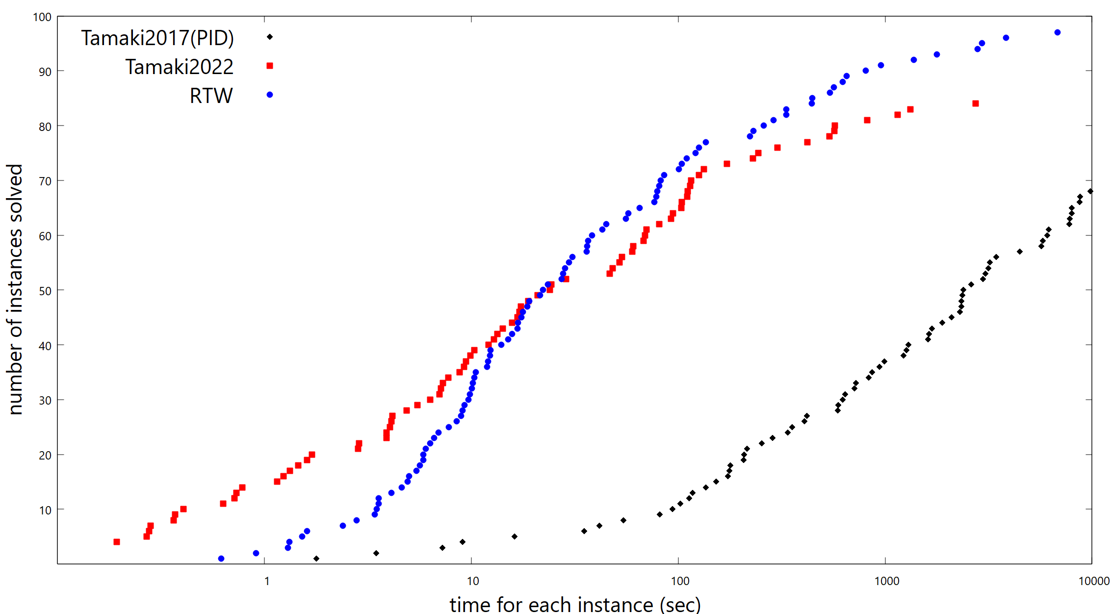
Experiments show that our algorithm drastically extends the scope of practically solvable instances. In particular, when applied to the 100 instances in the PACE 2017 bonus set, the number of instances solved by our implementation on a typical laptop, with the timeout of 100, 1000, and 10000 seconds per instance, are 72, 92, and 98 respectively, while these numbers are 11, 38, and 68 for Tamaki’s PID solver and 65, 82, and 85 for his new solver (SEA 2022).
keywords:
graph algorithm, treewidth, exact computation, BT dynamic programming, contraction, certifying algorithmscategory:
\relatedversion1 Introduction
Treewidth is a graph parameter introduced and extensively studied in the graph minor theory [14]. A tree-decomposition of graph is a tree with each node labeled by a vertex set of , called a bag, satisfying certain conditions (see Section 2) so that those bags form a tree-structured system of vertex-separators of . The width of a tree-decomposition is the maximum cardinality of a bag in minus one and the treewidth of graph is the smallest such that there is a tree-decomposition of of width .
The impact of the notion of treewidth on the design of combinatorial algorithms is profound: there are a huge number of NP-hard graph problems that are known to be tractable when parameterized by treewidth: they admit an algorithm with running time , where is the number of vertices, is the treewidth of the given graph, and is some typically exponential function (see [10], for example). Those algorithms typically perform dynamic programming based on the system of separators provided by the tree-decomposition. To make such algorithms practically useful, we need to compute the treewidth, or a good approximation of the treewidth, together with an associated tree-decomposition.
Computing the treewidth of a given graph is NP-complete [2], but is fixed-parameter tractable [14, 4]. In particular, the algorithm due to Bodlaender [4] runs in time linear in the graph size with a factor of . Unfortunately, this algorithm does not seem to run efficiently in practice.
In more practical approaches to treewidth computation, triangulations of graphs play an important role. A triangulation of graph is a chordal graph with and . For every tree-decomposition of , filling every bag of into a clique gives a triangulation of . Conversely, for every triangulation of , there is a tree-decomposition of in which every bag is a maximal clique of . Through this characterization of tree-decompositions in terms of triangulations, we can enumerate all relevant tree-decompositions by going through the total orderings on the vertex set, as each total ordering defines a triangulation for which the ordering is a perfect elimination order (see [7], for example). Practical algorithms in the early stage of treewidth research performed a branch-and-bound search over these total orderings [7]. Dynamic programming on this search space results in a time algorithms [5], which works well in practice for graphs with a small number of vertices. It should also be noted that classical upper bound algorithms, such as min-deg or min-fill, which heuristically choose a single vertex ordering defining a tree-decomposition, are fast and often give a good approximation of the treewidth in a practical sense [7].
Another important link between chordal graphs and treewidth computation was established by Bouchitté and Todinca [9]. They introduced the notion of potential maximal cliques (PMCs, see below in "Our approach" paragraph for a definition) and gave an efficient dynamic programming algorithm working on PMCs (BT dynamic programming) to find a minimal triangulation of the given graph that corresponds to an optimal tree-decomposition. They showed that their algorithm runs in polynomial time for many special classes of graphs. BT dynamic programming is also used in an exponential time algorithm for treewidth that runs in time [12].
BT dynamic programming had been considered mostly of theoretical interest until 2017, when Tamaki presented its positive-instance driven (PID) variant, which runs fast in practice and significantly outperforms previously implemented treewidth algorithms [18]. Further efforts on treewidth computation based on or around his approach have been made since then, with some incremental successes [17, 16, 19, 1].
In his most recent work [20], Tamaki introduced another approach to treewidth computation, based on the use of contractions to compute tight lower bounds on the treewidth. For edge of graph , the contraction of by , denoted by , is a graph obtained from by replacing by a new single vertex and let be adjacent to all neighbors of the ends of in . A graph is a contraction of if is obtained from by zero ore more successive contractions by edges. It is well-known and easy to see that for every contraction of . This fact has been used to quickly compute reasonably good lower bounds on the treewidth of a graph, typically to be used in branch-and-bound algorithms mentioned above [7, 8]. Tamaki [20] gave a heuristic method of successively improving contraction based lower bounds which, together with a separate heuristic method for upper bounds, quite often succeeds in computing the exact treewidth of instances that are hard to solve for previously published solvers.
Our approach
Our approach is based on the observation that contractions are useful not only for computing lower bounds but also for computing upper bounds. Suppose we have a tree-decomposition of of width for some edge of . Let be the vertex to which contracts. Replacing each bag of by , where if and otherwise, we obtain a tree-decomposition of of width , which we call the uncontraction of . In a fortunate case where every bag of with has , the width of is . To increase the chance of having such fortunate cases, we deal with a set of tree-decompositions rather than a single tree-decomposition. We represent such a set of tree-decompositions by a set of potential maximal cliques as follows.
A vertex set of is a potential maximal clique (PMC for short) if it is a maximal clique of some minimal triangulation of . Let denote the set of all PMCs of . For each , let denote the set of all tree-decompositions of whose bags all belong to . Let denote the smallest such that there is a tree-decomposition in of width ; we set if . Bouchitté and Todinca [9] showed that contains a tree-decomposition of width and developed a dynamic programming algorithm (BT dynamic programming) to find such a tree-decomposition. Indeed, as Tamaki [17] noted, BT dynamic programming can be used for arbitrary to compute in time linear in and polynomial in .
A set of PMCs is a particularly effective representation of a set of tree-decompositions for our purposes, because BT dynamic programming can be used to work on and find a tree-decomposition in that minimizes a variety of width measures based on bag weights. In our situation, suppose we have such that . Using appropriate bag weights, we can use BT dynamic programming to decide if contains such that the uncontraction of has width and find one if it exists.
These observation suggests a recursive algorithm for improving an upper bound on treewidth. Given graph and such that , the task is to decide if . Our algorithm certifies the YES answer by with . It uses heuristic methods to find such and, when this goal is hard to achieve, recursively solve the question if for edge of . Unless and hence , the recursive call returns such that . We use the method mentioned above to look for whose uncontraction has width . If we are successful, we are done for . Even when this is not the case, the uncontractions of tree-decompositions in may be useful for our heuristic upper bound method in the following manner.
In [17], Tamaki proposed a local search algorithm for treewidth in which a solution is a set of PMCs rather than an individual tree-decomposition and introduced several methods of expanding into in hope of having . His method compares favourably with existing heuristic algorithms but, like typical local search methods, is prone to local optima. To let the search escape from a local optimum, we would like to inject "good" PMCs to the current set . It appears that tree-decompositions in such that , where , are reasonable sources of such good PMCs: we uncontract into a tree-decomposition of and extract PMCs of from . Each such PMC appears in a tree-decomposition of width and may appear in a tree-decomposition of width . It is also important that is obtained, in a loose sense, independently of and not under the influence of the local optimum around which stays.
Our algorithm for deciding if interleaves the execution of a local search algorithm with recursive calls on for edges of and injects PMCs obtained from the results of the recursive calls. This process ends in either of the following three ways.
-
1.
The local search succeeds in finding with .
-
2.
A recursive call on finds that : we conclude that on the spot.
-
3.
Recursive calls have been tried for all edges and it is still unknown if . We invoke a conventional exact algorithm for treewidth to settle the question.
Note that, when the algorithm concludes that , there must be a contraction of somewhere down in the recursion path from such that Case 3 applies and the exact computation shows that . In this case, is a minimal contraction of that certifies , as the recursive calls further down from have shown for every edge of .
As the experiments in Section 11 show, this approach drastically extends the scope of instances for which the exact treewidth can be computed in practice.
Organization
To quickly grasp the main ideas and contributions of this paper, it is suggested to read the following sections first: Section 3 – Main algorithm, Section 6 – Uncontracting PMCs, Section 7 – Contracting PMCs, and Section 11 – Experiments (about 9 pages in total including the introduction), together with some parts of the preliminaries section as needed. Section 4 describes some details of the local search algorithm we use, namely heuristic PID. Sections 8, 9, and 10 describe additional techniques for speeding up the main algorithm. Sections 12 offers some concluding remarks.
The source code of the implementation of our algorithm used in the experiments is available at https://github.com/twalgor/RTW.
2 Preliminaries
Graphs and treewidth
In this paper, all graphs are simple, that is, without self loops or parallel edges. Let be a graph. We denote by the vertex set of and by the edge set of . As is simple, each edge of is a subset of with exactly two members that are adjacent to each other in . The complete graph on , denoted by , is a graph with vertex set in which every vertex is adjacent to all other vertices. The subgraph of induced by is denoted by . We sometimes use an abbreviation to stand for . A vertex set is a clique of if is a complete graph. For each , denotes the set of neighbors of in : . For , the open neighborhood of in , denoted by , is the set of vertices adjacent to some vertex in but not belonging to itself: .
We say that vertex set is connected in if, for every , there is a path in between and . It is a connected component or simply a component of if it is connected and is inclusion-wise maximal subject to this condition. We denote by the set of all components of . When the graph is clear from the context, we denote by . A vertex set is a separator of if has more than one component. A graph is a cycle if it is connected and every vertex is adjacent to exactly two vertices. A graph is a forest if it does not have a cycle as a subgraph. A forest is a tree if it is connected.
A tree-decomposition of is a pair where is a tree and is a family of vertex sets of , indexed by the nodes of , such that the following three conditions are satisfied. We call each the bag at node .
-
1.
.
-
2.
For each edge , there is some such that .
-
3.
For each , the set of nodes is connected in .
The width of this tree-decomposition is . The treewidth of , denoted by is the smallest such that there is a tree-decomposition of of width .
For each pair of adjacent nodes of a tree-decomposition of , let denote the subtree of consisting of nodes of reachable from without passing and let . Then, it is well-known and straightforward to show that and there are no edges between and ; is a separator of unless or . We say that uses separator if there is an adjacent pair such that . In this paper, we assume is connected whenever we consider a tree-decomposition of .
In this paper, most tree-decompositions are such that only if . Because of this, we use a convention to view a tree-decomposition of as a tree whose nodes are bags (vertex sets) of .
Triangulations, minimal separators, and Potential maximal cliques
Let be a graph and a separator of . For distinct vertices , is an - separator if there is no path between and in ; it is a minimal - separator if it is an - separator and no proper subset of is an - separator. A separator is a minimal separator if it is a minimal - separator for some .
Graph is chordal if every induced cycle of has exactly three vertices. is a triangulation of graph if it is chordal, , and . A triangulation of is minimal if it there is no triangulation of such that is a proper subset of . It is known (see [13] for example) that if is a minimal triangulation of then every minimal separator of is a minimal separator of . In fact, the set of minimal separators of is a maximal set of pairwise non-crossing minimal separators of , where two separators and cross each other if at least two components of intersects .
Triangulations and tree-decompositions are closely related. For a tree-decomposition of , let denote the graph obtained from by filling every bag of into a clique. Then, it is straightforward to see that is a triangulation of . Conversely, for each chordal graph , consider a tree on the set of all maximal cliques of such that if are adjacent to each other then is a minimal separator of . Such a tree is called a clique tree of . It is straightforward to verify that a clique tree of a triangulation of is a tree-decomposition of and that .
We call a tree-decomposition of minimal if it is a clique tree of a minimal triangulation of . It is clear that there is a minimal tree-decomposition of of width , since for every tree-decomposition of , there is a minimal triangulation of that is a subgraph of and every clique tree of has .
A vertex set is a potential maximal clique, PMC for short, of , if is a maximal clique in some minimal triangulation of . We denote by the set of all potential maximal cliques of . By definition, every bag of a minimal tree-decomposition of belongs to .
Bouchitté-Todinca dynamic programming
For each , say that admits a tree-decomposition of if every bag of belongs to . Let denote the set of all tree-decompositions of that admits and let denote the smallest such that there is of width ; we set if . The treewidth algorithm of Bouchitté and Todinca [9] is based on the observation that . Given , their algorithm first constructs and then search through by dynamic programming (BT dynamic programming) to find of width . As observed in [17], BT dynamic programming can be used to compute for an arbitrary subset of to produce an upper bound on . As we extensively use this idea, we describe how it works here.
Fix such that is non-empty. To formulate the recurrences in BT dynamic programming, we need some definitions. A vertex set of is a block if is connected and either is a minimal separator or is empty. As we are assuming that is connected, in the latter case. A partial tree-decomposition of a block in is a tree-decomposition of that has a bag containing , called the root bag of this partial tree-decomposition. Note that a partial tree-decomposition of block is a tree-decomposition of . For graph and block , let denote the set of all partial tree-decompositions of in all of whose bags belong to and, when this set is non-empty, let denote the smallest such that there is with ; if is empty we set .
A PMC of is a cap of block if and . Note that a cap of is a potential root bag of a partial tree-decomposition of . For each block , let denote the set of all caps of belonging to . Recall that, for each vertex set , denotes the set of components of . The following recurrence holds.
| (1) |
BT dynamic programming evaluates this recurrence for blocks in the increasing order of cardinality and obtains . Tracing back the recurrences, we obtain a tree-decomposition with .
Tamaki’s PID algorithm [18], unlike the original algorithm of Bouchitté and Todinca [9], does not construct before applying dynamic programming. It rather uses the above recurrence to generate relevant blocks and PMCs. More precisely, PID is for the decision problem whether for given and and it generates all blocks with using the recurrence in a bottom up manner. We have if and only if is among those generated blocks.
Contractors and contractions
To extend the notation of a contraction by an edge to a contraction by multiple edges, we define contractors. A contractor of is a partition of into connected sets. For contractor of , the contraction of by , denoted by , is the graph obtained from by contracting each part of to a single vertex, with the adjacency inherited from . For notational convenience, we also view a contractor as a mapping from to , the index set of the parts of the partition . In this view, the vertex set of is and for each is the vertex of into which is contracted. For each , is the part of the partition that contracts to . For , we define .
3 Main algorithm
The pseudo code in Algorithm 1 shows the main iteration of our treewidth algorithm. It starts from a greedy upper bound and repeatedly improves the upper bound by algorithm RTW. The call , where and , decides if . If , it returns YES with certificate such that ; otherwise it returns NO with certificate , a minimal contraction of such that .
The pseudo code in Algorithm 2 describes RTW in its basic form. We sketch here the functions of subalgorithms used in this algorithm. More details can be found in subsequent sections.
Our method of local search in the space of sets of PMCs is a heuristic variant, which we call HPID, of the PID algorithm due to Tamaki [18]. PID constructs partial tree-decompositions of width using the recurrence of BT dynamic programming in a bottom up manner to exhaustively generate all partial tree-decompositions of width , so that we have a tree-decomposition of width if and only if . HPID uses the same recurrence to generate partial tree-decompositions of width but the aim is to quickly generate a tree-decomposition of of width and the generation order it employs does not guarantee exhaustive generation. The state of HPID computation is characterized by the set of root bags of the generated partial tree-decompositions. Recall that the bags of the set of partial tree-decompositions generated by the BT recurrence are PMCs, so . Using BT dynamic programming, we can reconstruct the set of partial tree-decompositions from , if needed, in time linear in and polynomial in . Thus, we may view HPID as performing a local search in the space of sets of PMCs. This view facilitates communications between HPID and external upper bound heuristics. Those communications are done through the following operations.
We consider each invocation of HPID as an entity having a state. Let denote such an invocation instance of HPID for and . Let denote the set of PMCs that are root bag of the partial tree-decompositions generated so far by . The following operations are available.
-
returns .
-
returns the set of PMCs that are the root bags of the partial tree-decompositions of width generated so far by .
-
updates to and updates the set of partial tree-decompositions by BT dynamic programming.
-
generates more partial tree-decompositions under the specified budget, in terms of the number of search step spent for the generation.
-
exhaustively generates remaining partial decompositions of width , thereby deciding if .
See Section 4 for details of these procedures.
We use two additional procedures.
-
, where is an edge of and , returns such that and possibly
-
, where is an edge of and , returns such that and possibly
Given these procedures, RTW works as follows. It receives , , and such that and creates an HPID instance for and and let it import . If it turns out that at this point, then RTW returns YES with , a subset of such that , as the certificate. Otherwise, it orders the edges of in such a way to increase the chance of having an edge width early in the list if any. Then it iterates over those edges. To process it makes a recursive call where is obtained by "contracting" . If the result is negative, the answer of is also negative with the same certificate. If the result is positive with , then is "uncontracted" to , which is imported to . Then it lets advance its PID state under a budget proportional to . If succeeds in finding tree-decompositions of of width , then RTW returns YES with the certificate constructed by . Otherwise, it proceeds to the next edge. When it has tried all edges without resolving the question, it lets finish the exhaustive generation of partial tree-decompositions to answer the question. If it turns out that , it returns YES with the certificate provided by . Otherwise it returns NO with the certificate being itself.
The correctness of this algorithm can be proved by straightforward induction and does not depend on the procedures , , or except that the procedure must return such that as promised. On the other hand, practical efficiency of this algorithm heavily depends on the performances of these procedures. If they collectively work really well, then we expect that the for loop would exit after trying only a few edges, assuming , and would be called only if and for every edge . On the other extreme of perfect incapability of these procedures, the for loop would always run to the end and would be called in every call of , making the recursion totally meaningless. Our efforts are devoted to developing effective methods for these procedures.
4 Heuristic PID
In this section, we give some details of the HPID algorithm. In particular, we describe in some details how the procedures and work.
We first describe how we use Recurrence 1 to generate a new partial tree-decomposition from existing ones. The method basically follows that of PID [18] but there are some differences. The most important difference is in the manners we turn tree-decompositions into rooted tree-decompositions, which is done in order to restrict partial tree-decompositions to be generated. In the original PID, the choice of roots heavily depends on the total order assumed on . For the sake of interactions of HPID with other upper bound components through PMCs, we prefer the choice to depend less on the vertex order and thus be fairer for vertices.
Fix and . We assume a total order on and say that is larger then if or and is lexicographically larger than . We say that a block of is feasible if . We use recurrence 1, with set to , to generate feasible blocks. Our goal is to see if is feasible and, to this end, it turns out that we do not need to generate all feasible blocks: it suffices to generate only small feasible blocks except for itself, where a block is small if there is some block with such that .
To see this, we construct rooted tree-decompositions from minimal triangulations of . Let be a minimal triangulation of . We define a rooted tree on the set of maximal cliques of , which may be denoted by because every PMC of is a maximal clique. For and a minimal separator , let denote the full component of that intersects . Note that is a block since is a minimal separator. For such that is a separator of , let denote the inclusion-minimal minimal separator of contained in . Such an inclusion minimal separator is unique: if distinct are both inclusion-minimal separators, then both of the strict inclusions of and must hold, which is impossible.
We first define a dag on : for distinct there, has an edge from to if is a separator of and is larger than .
Proposition 4.1.
is acyclic.
Proof 4.2.
Suppose, for contradiction, there is a directed cycle in and let , …, , be the shortest such. Let . It cannot be that , since then we would have both and .
Let be such that and . Such must exist since and . Let . Since every block of is either contained in or disjoint from it, we have and . Since separates these blocks, we must have . Since and are both inclusion-minimal, we must have as argued above. Then, we have and therefore we have an edge from to , contradicting the assumption that our directed cycle is the shortest.
Now we construct a directed tree on with a unique sink. As is acyclic, it has a sink . Let denote the set of components of . Each is a block since is a minimal-separator. Let denote the set of maximal cliques of contained in . Note that , , partitions . For each such , we construct a directed tree on with unique sink such that has an edge from to . Combining , , with these edges from to , we obtain . It remains to show how we construct .
Observe that every is small. For each small block , we construct a directed tree on with sink such that inductively as follows. Let denote the set of caps of belonging to . By the definition of caps, each satisfies and . The subgraph of induced by has a sink since is acyclic. Let denote the set of blocks of that are components of . For each , we have and, moreover, for each block of , we have . Therefore, since there is a block of such that as is small, we have for each , that is, is small. By the induction hypothesis, we have a directed tree on with sink such that , for each . Combining , , with an edge from each to , we obtain the desired directed tree .
Let be a minimal triangulation of such that . In view of the existence of the rooted clique tree of , feasibility of can be determined by generating only small feasible blocks using recurrence 1 and then seeing if the same recurrence can be used to show . Thus, each HPID instance maintains a set set of small feasible blocks. To generate a new feasible block to add to , it invokes a backtrack search procedure on a block which enumerates such that
-
1.
and is the largest block in and
-
2.
there is a block that is either small or is equal to and a PMC such that .
For each such found, we add to since the recurrence 1 shows that is feasible.
Procedure uses this search procedure as follows. It uses a priority queue of small feasible blocks, in which larger blocks are given higher priority. It first put all blocks in to . Then, it dequeues a block , call , and add newly generated feasible blocks to . This is repeated until either is empty or the cumulative number of search steps exceeds . Because of the queuing policy, there is a possibility of found feasible, when it is indeed feasible, even with a small budget.
Procedure works similarly, except that smaller blocks are given higher priority in the queue and the budget is unlimited, to generate all small feasible blocks and if it is feasible.
An alternative way to to implement the procedure is to call another exact treewidth algorithm based on BT dynamic programming, such as SemiPID [16], to decide if is feasible. The implementation used in our experiment uses this alternative method.
5 Minimalizing tree-decompositions
Given a graph and a triangulation of , minimalizing means finding a minimal triangulation of such that . Minimalizing a tree-decomposition of means finding a minimal tree-decomposition of whose bags are maximal cliques of the minimalization of . We want to minimalize a tree-decomposition for two reasons. One is our decision to represent a set of tree-decompositions by a set of PMCs. Whenever we get a tree-decomposition by some method that may produce non-minimal tree-decompositions, we minimalize it to make all bags PMCs. Another reason is that minimalization may reduce the width. We have two procedures for minimalization. When the second reason is of no concern, we use which is an implementation of one of the standard triangulation minimalization algorithm due to Blair et al [3]. When the second reason is important, we use , which finds a minimalization of of the smallest width. This task is NP-hard, but the following algorithm works well in practice.
Say a minimal separator of is admissible for if it is a clique of . Observe that, for every minimalization of , every separator used by is a minimal separator of admissible for . We first construct the set of all minimal separators of admissible for . Then we apply the SemiPID variant of BT dynamic programming, due to Tamaki [16], to this set and obtain a tree-decomposition of the smallest width, among those using only admissible minimal separators. Because of the admissibility constraint, the number of minimal separators is much smaller and both the enumeration part and the SemiPID part run much faster in practices than in the general case without such constraints.
6 Uncontracting PMCs
In this section, we develop an algorithm for procedure . In fact, we generalize this procedure to , where the third argument is a general contractor of .
Given a graph , , and a contractor of , we first find tree-decompositions that minimize . This is done by BT dynamic programming over , using bag weights defined as follows. For each weight function that assigns weight to each vertex set , define the width of tree-decomposition with respect to , denoted by , to be the maximum of over all bags of . Thus, if is defined by then . A natural choice for our purposes is to set . Then, the width of a tree decomposition of with respect to this bag weight is . Therefore, BT dynamic programming with this weight function gives us the desired tree-decomposition in .
We actually use a slightly modified weight function, considering the possibility of reducing the weight of by minimalization.
Let and a bag of . If is a PMC of , then every minimalization of must contain as a bag. Therefore, if then it is impossible that the width of is reduced to by minimalization. On the other hand, if is not a PMC, then no minimalization of has has a bag and there is a possibility that there is a minimalization of of width even if . These considerations lead to the following definition of our weight function .
| (2) | |||||
| (3) |
Algorithm 3 describes the main steps of procedure .
7 Contracting PMCs
The algorithm for procedure is similar to that for . Given a graph , , and a contractor of , we first find tree-decompositions that minimize . This is done by BT dynamic programming with the following weight function .
Then, we minimalize those tree-decompositions and collect the bags of those minimalized tree-decompositions.
8 Safe separators
Bodlaender and Koster [6] introduced the notion of safe separators for treewidth. Let be a separator of a graph . We say that is safe for treewidth, or simply safe, if . As every tree-decomposition of must have a bag containing , is the larger of and , where ranges over all the components of . Thus, the task of computing reduces to the task of computing for every component of . The motivation for looking at safe separators of a graph is that there are sufficient conditions for a separator being safe and those sufficient conditions lead to an effective preprocessing method for treewidth computation. We use the following two sufficient conditions.
A vertex set of is an almost-clique if is a clique for some . Let be a vertex set of . A contractor of is rooted on if, for each part of , .
Theorem 8.1.
Bodlaender and Koster [6]
-
1.
If is an almost-clique minimal separator of , then is safe.
-
2.
Let be a lower bound on . Let be connected and let . Suppose (1) and (2) has a contractor rooted on such that is a complete graph. Then, is safe.
We use safe separators both for preprocessing and during recursion. For preprocessing, we follow the approach of [19]: to preprocess , we fix a minimal triangulation of and test the sufficient conditions in the theorem for each minimal separator of . Since deciding if the second condition holds is NP-complete, we use a heuristic procedure. Let be the set of all minimal separators of that are confirmed to satisfy the first or the second condition of the theorem. Let be a tree-decomposition of that uses all separators of but no other separators. Then, is what is called a safe-separator decomposition in [6]. A tree-decomposition of of width can be obtained from by replacing each bag of by a tree-decomposition of , the graph obtained from the subgraph of induced by by filling the neighborhood of every component of into a clique.
Safe separators are also useful during the recursive computation. Given , we wish to find a contractor of such that , so that we can safely recurse on . The second sufficient condition in Theorem 8.1 is useful for this purpose. Let , , and be as in the condition. We construct such that as follows. The proof of this sufficient condition is based on the fact that we get a clique on when we apply the contractor on . Thus, we may define a contractor on such that . As each tree-decomposition of can be extended to a tree-decomposition of , using the tree-decomposition of of width at most , we have = as desired. When the recursive call on returns a certificate such that , we need to "uncontract" into a such that . Fortunately, this can be done without invoking the general uncontraction procedure. Observe first that each PMC in naturally corresponds to a PMC of , which in turn corresponds to a PMC of contained in . Let be the set of those PMCs of to which a PMC in corresponds in that manner. Let be such that . Similarly as above, each PMC of corresponds to a PMC of contained . Let denote the set of those PMCs of to which a PMC in corresponds. As argued above, a tree-decomposition in of and a tree-decomposition in of can be combined into a tree-decomposition belonging to of width . Thus, is a desired certificate for .
9 Edge ordering
We want an edge such that , if any, to appear early in our edge order. Heuristic criteria for such an ordering have been studied in the classic work on contraction based lower bounds [8]. Our criterion is similar to those but differs in that it derives from a special case of safe separators. The following is simple corollary of Theorem 8.1.
Proposition 9.1.
Let be an edge of and let . Suppose is a clique of . Then, we have .
If satisfies the above condition, then we certainly put first in the order. Otherwise, we evaluate in terms of its closeness to this ideal situation. Define the deficiency of graph , denoted by , to be the number of edges of its complement graph. For each ordered pair of adjacent vertices of , let denote . Note that means that the condition of the above proposition is satisfied with . Thus, we regard preferable if either or is small. We relativize the smallness with respect to the neighborhood size, so the value of edge is . We order edges so that this value is non-decreasing.
10 Suppressed edges
Consider the recursive call on from the call of RTW on , where is an edge of . Suppose there is an ancestor call on such that and edge of such that maps the ends of to the ends of . If the call on has been made and it is known that then we know that , since is a contraction of . In this situation, we that is suppressed by the pair . We may omit the recursive call on without compromising the correctness if is suppressed. For efficiency, however, it is preferable to obtain the certificate for and feed the uncontraction of to the HPID instance on to help progress. Fortunately, this can be done without making the recursive call on as follows. Suppose is suppressed by and let such that . Let be the contractor of such that : such is straightforward to obtain from . Letting , we obtain such that .
11 Experiments
We have implemented RTW and evaluated it by experiments. The computing environment for our experiments is as follows. CPU: Intel Core i7-8700K, 3.70GHz; RAM: 64GB; Operating system: Windows 10Pro, 64bit; Programming language: Java 1.8; JVM: jre1.8.0_271. The maximum heap size is set to 60GB. The implementation uses a single thread except for additional threads that may be invoked for garbage collection by JVM.
Our primary benchmark is the bonus instance set of the exact treewidth track of PACE 2017 algorithm implementation challenge [11]. This set, consisting of 100 instances, is intended to be a challenge for future implementations and, as a set, are hard for the winning solvers of the competition. Using the platform of the competition, about half of the instances took more than one hour to solve and 15 instances took more than a day or were not solvable at all.
We have run our implementation on these instances with the timeout of 10000 seconds each. For comparison, we have run Tamaki’s PID solver [18], which is one of the PACE 2017 winners, available at [15] and his new solver [20] available at [21]. Figure 1 summarizes the results on the bonus set. In contrast to PID solver which solves only 68 instances within the timeout, RTW solves 98 instances. Moreover, it solve 72 of them in 100 seconds and 92 of them in 1000 seconds. Thus, we can say that our algorithm drastically extends the scope of practically solvable instances. Tamaki’s new solver also quickly solves many instances that are hard for PID solver and is indeed faster then RTW on many instances. However, its performance in terms of the number of instances solvable in practical time is inferior to RTW.
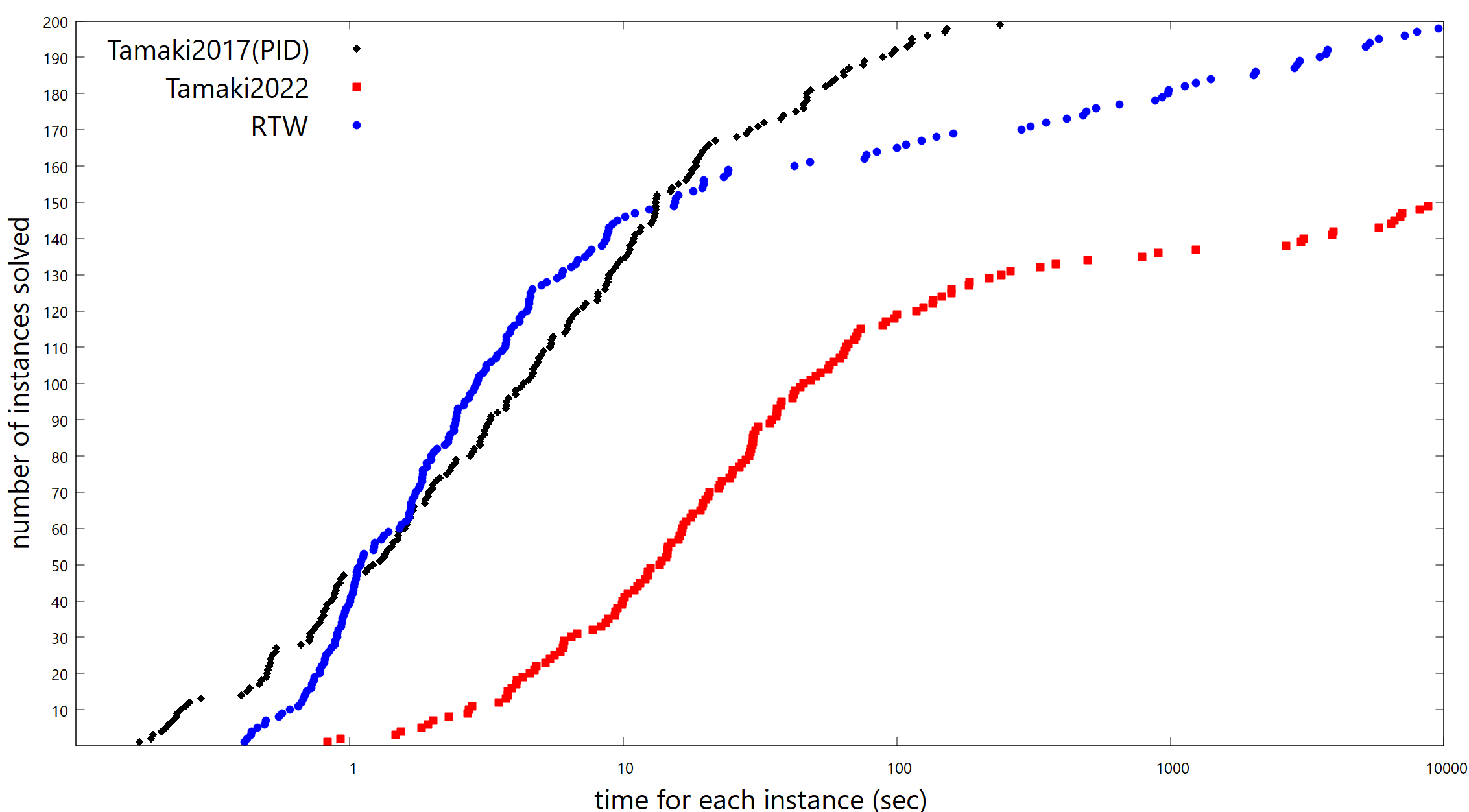
We have also run the solvers on the competition set of the exact treewidth track of PACE 2017. This set, consisting of 200 instances, is relatively easy and the two winning solvers of the competitions solved all of the instances within the allocated timeout of 30 minutes for each instance. Figure 2 summarizes the results on the competition set. Somewhat expectedly, PID performs the best on this instance set. It solves almost all instances in 200 seconds for each instance, while RTW fails to do so on about 30 instances. There are two instances that RTW fails to solve in 10000 seconds and one instance it fails to solve at all. Tamaki’s new solver shows more weakness on this set, failing to sove about 50 instances in the timeout of 10000 seconds.
These results seem to suggest that RTW and PID should probably complement each other in a practical treewidth solver.
12 Conclusions and future work
We developed a treewdith algorithm RTW that works recursively on contractions. Experiments show that our implementation solves many instances in practical time that are hard to solve for previously published solvers. RTW, however, does not perform well on some instances that are easy for conventional solvers such as PID. A quick compromise would be to run PID first with an affordable timeout and use RTW only when it fails. It would be, however, interesting and potentially fruitful to closely examine those instances that are easy for PID and hard for RTW and, based on such observations, to look for a unified algorithm that avoids the present weakness of RTW.
References
- [1] Ernst Althaus, Daniela Schnurbusch, Julian Wüschner, and Sarah Ziegler. On tamaki’s algorithm to compute treewidths. In 19th International Symposium on Experimental Algorithms (SEA 2021). Schloss Dagstuhl-Leibniz-Zentrum für Informatik, 2021.
- [2] Stefan Arnborg, Derek G Corneil, and Andrzej Proskurowski. Complexity of finding embeddings in a -tree. SIAM Journal on Algebraic Discrete Methods, 8(2):277–284, 1987.
- [3] Jean RS Blair, Pinar Heggernes, and Jan Arne Telle. A practical algorithm for making filled graphs minimal. Theoretical Computer Science, 250(1-2):125–141, 2001.
- [4] Hans L Bodlaender. A linear-time algorithm for finding tree-decompositions of small treewidth. SIAM Journal on computing, 25(6):1305–1317, 1996.
- [5] Hans L Bodlaender, Fedor V Fomin, Arie MCA Koster, Dieter Kratsch, and Dimitrios M Thilikos. On exact algorithms for treewidth. In Algorithms–ESA 2006: 14th Annual European Symposium, Zurich, Switzerland, September 11-13, 2006. Proceedings, pages 672–683. Springer, 2006.
- [6] Hans L Bodlaender and Arie MCA Koster. Safe separators for treewidth. Discrete Mathematics, 306(3):337–350, 2006.
- [7] Hans L Bodlaender and Arie MCA Koster. Treewidth computations i. upper bounds. Information and Computation, 208(3):259–275, 2010.
- [8] Hans L Bodlaender and Arie MCA Koster. Treewidth computations ii. lower bounds. Information and Computation, 209(7):1103–1119, 2011.
- [9] Vincent Bouchitté and Ioan Todinca. Treewidth and minimum fill-in: Grouping the minimal separators. SIAM Journal on Computing, 31(1):212–232, 2001.
- [10] Marek Cygan, Fedor V Fomin, Łukasz Kowalik, Daniel Lokshtanov, Dániel Marx, Marcin Pilipczuk, Michał Pilipczuk, and Saket Saurabh. Parameterized algorithms. Springer, 2015.
- [11] Holger Dell, Christian Komusiewicz, Nimrod Talmon, and Mathias Weller. The pace 2017 parameterized algorithms and computational experiments challenge: The second iteration. In 12th International Symposium on Parameterized and Exact Computation (IPEC 2017). Schloss Dagstuhl-Leibniz-Zentrum fuer Informatik, 2018.
- [12] Fedor V Fomin and Yngve Villanger. Treewidth computation and extremal combinatorics. Combinatorica, 32(3):289–308, 2012.
- [13] Pinar Heggernes. Minimal triangulations of graphs: A survey. Discrete Mathematics, 306(3):297–317, 2006.
- [14] Neil Robertson and Paul D. Seymour. Graph minors. ii. algorithmic aspects of tree-width. Journal of algorithms, 7(3):309–322, 1986.
- [15] Hisao Tamaki. PID. https://github.com/TCS-Meiji/PACE2017-TrackA, 2017. [github repository].
- [16] Hisao Tamaki. Computing treewidth via exact and heuristic lists of minimal separators. In International Symposium on Experimental Algorithms, pages 219–236. Springer, 2019.
- [17] Hisao Tamaki. A heuristic use of dynamic programming to upperbound treewidth. arXiv preprint arXiv:1909.07647, 2019.
- [18] Hisao Tamaki. Positive-instance driven dynamic programming for treewidth. Journal of Combinatorial Optimization, 37(4):1283–1311, 2019.
- [19] Hisao Tamaki. A heuristic for listing almost-clique minimal separators of a graph. arXiv preprint arXiv:2108.07551, 2021.
- [20] Hisao Tamaki. Heuristic Computation of Exact Treewidth. In Christian Schulz and Bora Uçar, editors, 20th International Symposium on Experimental Algorithms (SEA 2022), volume 233 of Leibniz International Proceedings in Informatics (LIPIcs), pages 17:1–17:16, Dagstuhl, Germany, 2022. Schloss Dagstuhl – Leibniz-Zentrum für Informatik. URL: https://drops.dagstuhl.de/opus/volltexte/2022/16551, doi:10.4230/LIPIcs.SEA.2022.17.
- [21] Hisao Tamaki. twalgor/tw. https://github.com/twalgor/tw, 2022. [github repository].