Self-Tuning PID Control via a Hybrid Actor-Critic-Based Neural Structure for Quadcopter Control

Abstract

Proportional-Integrator-Derivative (PID) controller is used in a wide range of industrial and experimental processes. There are a couple of offline methods for tuning PID gains. However, due to the uncertainty of model parameters and external disturbances, real systems such as Quadrotors need more robust and reliable PID controllers. In this research, a self-tuning PID controller using a Reinforcement-Learning-based Neural Network for attitude and altitude control of a Quadrotor has been investigated. An Incremental PID, which contains static and dynamic gains, has been considered and only the variable gains have been tuned. To tune dynamic gains, a model-free actor-critic-based hybrid neural structure was used that was able to properly tune PID gains, and also has done the best as an identifier. In both tunning and identification tasks, a Neural Network with two hidden layers and sigmoid activation functions has been learned using Adaptive Momentum (ADAM) optimizer and Back-Propagation (BP) algorithm. This method is online, able to tackle disturbance, and fast in training. In addition to robustness to mass uncertainty and wind gust disturbance, results showed that the proposed method had a better performance when compared to a PID controller with constant gains.

I Introduction

Due to their low cost, simple mechanical structure, vertical take-off and landing capabilities, and high maneuverability, quadcopters are applicable in a wide range of industrial processes such as agriculture, search and rescue, inspection, and surveillance [1]. Because of the coupling among actuators and the uncertainty of external disturbances, they have a highly nonlinear dynamic system. That is why the role of attitude control in quadcopter trajectory tracking and maneuvering is of paramount importance. In [2], a variety of control algorithms were executed and showed that none of them can meet the requirements, even though hybrid methods have better adaptability and robustness to pass disturbances.

The PID controller is used extensively in real industrial systems due to its simplicity and ease of implementation. However, the accuracy of this controller is highly dependent on its gains and the system model. In high-order nonlinear systems, parameter uncertainties and external disturbances can reduce the performance of the PID controller. Conventional offline tuning methods are not efficient for such systems [3]. To achieve acceptable performance in nonlinear systems, it is better to use online methods such as Adaptive Control, Fuzzy Systems, and Neural Networks (NN) [4, 5, 6, 7, 8]. NNs are capable of solving non-trivial problems efficiently and approximating high-order nonlinear functions [9]. Furthermore, Reinforcement Learning (RL) methods, which use NNs in their structures, have demonstrated their ability and, in some cases, even outperform humans. RL algorithms are semi-supervised learning methods that employ an agent to learn by interacting with an environment. RL has considerable utility in self-tuning PID control and is capable of doing so without human designer intervention. For example, the Q-learning algorithm has been employed to tune PID gains [10, 11]. However, this algorithm cannot take continuous actions and requires a powerful processor and memory for improved accuracy. Additionally, using Actor-Critic methods, an agent can generate continuous actions (control signals), and more importantly, these methods are online and NN-based. In [12], a Radial Basis Function (RBF) NN was employed for actor policy and critic value function approximation, demonstrating that this algorithm can track a complex trajectory. Moreover, Deep Deterministic Policy Gradient (DDPG) is utilized in PID tuning [13, 14], which has offline training and necessitates a powerful processor. However, using DDPG, the trained model may lose its performance in a real system with environmental disturbances. In [15], Asynchronous Advantage Actor Critic (A3C) was employed for PID tuning, which can learn multi-actor and critic as workers. Results demonstrated that this method enhanced PID performance.

In this research, a new structure for tuning PID gains is introduced using NNs, taking advantage of recent algorithms that can perform both self-tuning PID and system identification. This fast and online method does not require a high-capacity memory, a powerful processor, or offline training. The Adaptive Momentum (ADAM) optimizer is used to update network weights with the Back Propagation algorithm [16]. ADAM is fast, efficient in deep networks, and capable of bypassing shallow local minimums. To evaluate the efficiency of our method, we investigate its performance when faced with mass uncertainty and wind gust disturbances.

In the following sections, we describe the dynamical modeling of a Quadrotor and PID control in Section II. In Section III, we design a hybrid neural structure for online PID gain tuning, followed by optimization. We perform comparative numerical simulations to demonstrate the effectiveness of the proposed controller in Section IV. Finally, we summarize our conclusions and contributions in Section V.

II Dynamic Modeling and PID Control Method

Quadcopter (as shown in Fig. 1) is an under-actuated system with four control inputs ($u_{1},u_{2},u_{3},u_{4}$) and six degrees of freedom (DOFs), including position ($x,y,z$) and attitude ($\phi,\theta,\psi$). Due to the nonlinearities of the quadcopter system and the complexity of environmental situations, it is nearly impossible to accurately model this robot. In such cases, system identification using methods such as NNs can efficiently estimate the states of the system. Therefore, our control method does not require a precise model and only needs instantaneous inputs and outputs of the system.

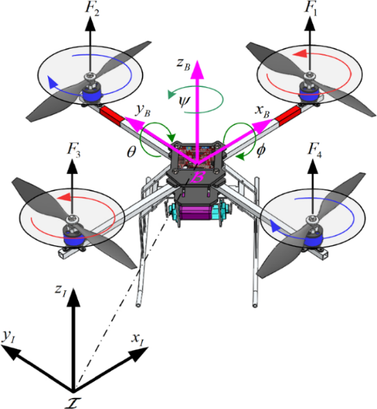
Figure 1: Quadcopter schematic

Therefore, in this research, a simple mathematical model [17] is used with known parameters only for simulating the real system without noise. In fact, we assume that we do not know the parameters of the system and estimate the states using corresponding control inputs and recent states. The governing equations are shown in Eq. 1. In this set of equations, $x,y,z$ are the positions of the center of gravity related to the reference coordinates $x_{I},y_{I},z_{I}$, and $\phi,\theta,\psi$ are the rotational angles around $x_{B},y_{B},z_{B}$.

$$\ddot{\phi} =\dot{\theta}\dot{\psi}\frac{J_{y}-J_{z}}{J_{x}}+\frac{l}{J_{x}}u_{2}$$ (1)

$$\ddot{\theta} =\dot{\phi}\dot{\psi}\frac{J_{z}-J_{x}}{J_{y}}+\frac{l}{J_{y}}u_{3}$$

$$\ddot{\psi} =\dot{\phi}\dot{\theta}\frac{J_{x}-J_{y}}{J_{z}}+\frac{1}{J_{z}}u_{4}$$

$$\ddot{z} =\frac{u_{1}}{m}cos\phi cos\theta-g$$

$$\ddot{x} =\frac{u_{1}}{m}(cos\phi sin\theta cos\psi+sin\phi sin\psi)$$

$$\ddot{y} =\frac{u_{1}}{m}(cos\phi sin\theta sin\psi-sin\phi cos\psi)$$

where $m,g,l$ are the total mass of robot, gravity, and quadcopter arm, and also $J_{x},J_{y},J_{z}$ are moments of innertia around body coordinates, respectively. Control inputs (Eq. 2) are combination of squared motor angular velocities ($\Omega_{1},\Omega_{2},\Omega_{3},\Omega_{4}$).

$$u_{1} =b(\Omega_{1}^{2}+\Omega_{2}^{2}+\Omega_{3}^{2}+\Omega_{4}^{2})$$ (2)

$$u_{2} =b(\Omega_{4}^{2}-\Omega_{2}^{2})$$

$$u_{3} =b(\Omega_{3}^{2}-\Omega_{1}^{2})$$

$$u_{4} =d(\Omega_{4}^{2}+\Omega_{2}^{2}-\Omega_{1}^{2}+\Omega_{3}^{2})$$

where $b$ and $d$ are thrust and torque coefficients. Now, we should determine control inputs using PID control algorithm in an online manner. Firstly, static PID gains are chosen with trial and error or Ziegler-Nichols method in which system reach credible stability. What is more, attained gains will not change during each mission. Having tuned dynamic gains using the proposed method, they are added to corresponding static gains. Thus, according to the following equation, each control input ($u_{1},u_{2},u_{3},u_{4}$) is the summation of corresponding static and dynamic gain inputs.

$$u_{(}t)=u_{sg}(t)+u_{dg}(t)$$ (3)

in which,

$$u_{sg}(t) =K_{p}^{s}e(t)+K_{i}^{s}\int_{0}^{t}e(\tau)\,d\tau+K_{d}^{s}\dot{e}(t)$$ (4)

$$u_{dg}(t) =K_{p}^{d}e(t)+K_{i}^{d}\int_{0}^{t}e(\tau)d\tau+K_{d}^{d}\dot{e}(t)$$

where $K_{p}^{s},K_{i}^{s},K_{d}^{s}$ are constant and determined in advance and $K_{p}^{d},K_{i}^{d},K_{d}^{d}$ are tuned using a neural network in which is based on actor-critic method. This method will be elaborated upon in the rest of the paper.

III Network Structure

The proposed method consists of two parts. The first part is self-tuning PID, and the second part is system identification using neural networks (NNs). In the first part, a NN is designed to tune dynamic PID gains. In the next step, the control input is computed by externally injecting PID errors to the network. Obtaining the control input in each step, it is fed to the system identification net when accompanied by recent outputs. This network estimates the new output of the system using an Actor-Critic structure. In fact, the whole identification net is composed of two networks. The first one is an Actor network that tries to identify the actual output of the system. Meanwhile, the second net, the Critic network, computes the value function of the net inputs (environment states) and shows the value of the actor’s action in the current state.

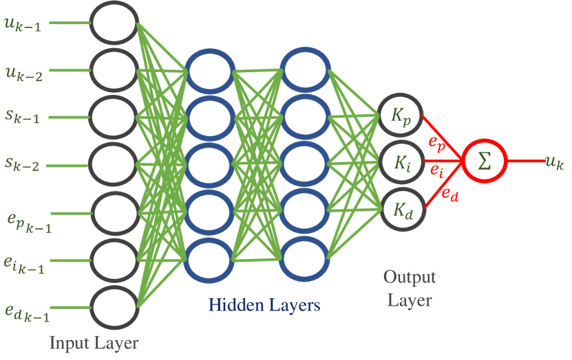
Figure 2: Self-tuning PID neural network. Inputs are current control inputs, cerrent states, and PID errors. Hidden layers and output layer activation functions are sigmoid and tanh respectively.

Considering Fig. 2, $Sigmoid$ activation function is used in hidden layers, whereas $Tanh$ utilized in the PID gains layer. Finally, dynamic PID gains ($K_{n}^{d}$) are computed using the following equation.

$$K_{n}^{d}(k)=f_{n}( u(k-1),u(k-2),s(k-1),s(k-2),$$ (5)

$$e_{p}(k-1),e_{i}(k-1),e_{d}(k-1))$$

where $n=p,i,d$ and $f_{n}(.)$ is a nonlinear function with quite a few weights and biases which are initialized in a bound near zero. In the identification net, actor network has two outputs, an average ($\mu$) and a variance ($\sigma$). The outputs of the actor net are fed into a normal distribution equation ($\mathcal{N}(\mu,\sigma^{2})$) and using normal distribution of actor outputs, a sample is taken randomly (Fig. 4).

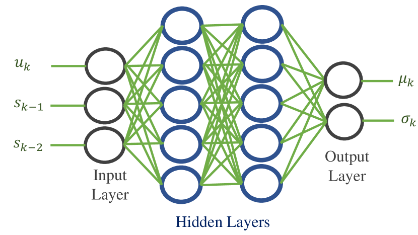
Figure 3: Actor network. Net inputs are current control input and current states and activations function is sigmoid for hidden layers.

where $s_{m}$ is an estimation of each state of the quadcopter (attitudes and altitude). This sample is the final output of actor network and we expect it to track the actual output of the system.

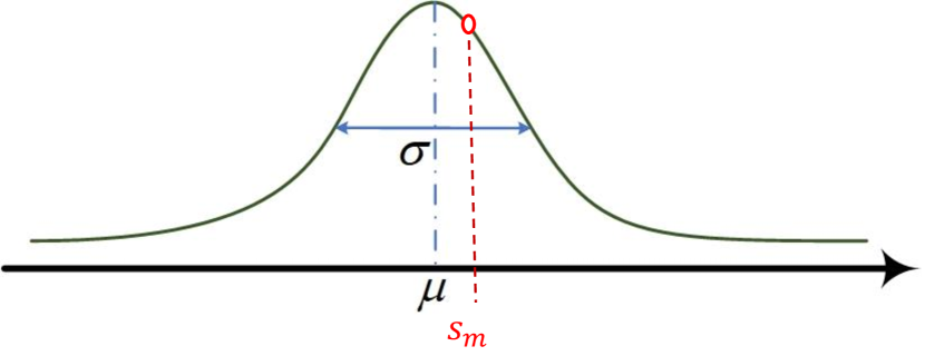
Figure 4: Guassian normal distrbution. The final output of actor network is taken from this distribution randomly.

Critic has to estimate the value function ($v$) using states (control input and recent outputs) and by doing so, it gives the actor a feedback to perform better than before.

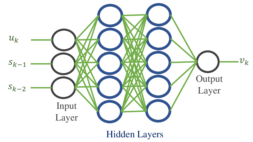
Figure 5: Critic network. The inputs of the net are current input and states and activations function is sigmoid. The output is value function.

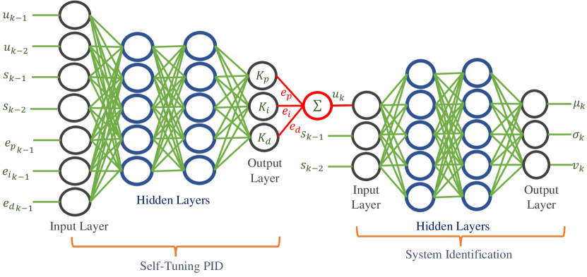
Figure 6: Total network. The left network tunes PID gains for each state of quadcopter and computes pertaining control input and the right net is actor-critic which estimates each state.

Finally, the outputs of the system identification network will be obtained using the following equations.

$$\mu(k) =f_{\mu}(u(k),s(k-1),s(k-2))$$ (6)

$$\sigma(k) =f_{\sigma}(u(k),s(k-1),s(k-2))$$ (7)

$$v(k) =f_{v}(u(k),s(k-1),s(k-2))$$ (8)

where $f_{\mu}(.),f_{\sigma}(.)$ are the corresponding functions of Actor, and $f_{v}(.)$ is that of Critic. Designing the self-tuning PID, Actor, and Critic networks individually, it is now time to connect the networks to work alongside each other to achieve the final objective of self-tuning after system identification. Therefore, we connect the self-tuning PID network to the system identification net in series (Fig. 6). By doing so, the final output of the former network will be fed into the latter one, resulting in the formation of a general uniform network. The inputs of the network are control inputs, current states, and PID errors. Eventually, the outputs are the estimations of each state and the value function of network inputs. With all of this in mind, we do not need a model of the system, thereby making the method a model-free one.

IV Optimization

After designing the network structure and initialization of weights and biases, the net parameters have to be adjusted using an optimizer. The actor’s goal is output estimation or minimization of the estimation error ($s_{m}-s$) and critic should minimize Temporal Difference error ($\delta_{TD}$) [18]. $\delta_{TD}$ is computed using the following equation.

$$\delta_{TD}=R_{k+1}+\gamma v_{k+1}-v_{k}$$ (9)

where $\gamma$ and $R_{k+1}$ are discount factor and reward function and $v_{k}$ and $v_{k+1}$ are value function in step $k$ and the next one. Reward function is defined in a quadratic form so that the less absolute error, error-rate, and control input, the more reward, according to the following equation.

$$R_{k+1}=-r_{1}(s_{m}-s)^{2}-r_{2}(\dot{s}_{m}-\dot{s})^{2}-r_{3}u^{2}$$ (10)

where $r_{1},r_{2},r_{3}$ are arbitrary reward coeficients and $u$ is the control signal. Finally, a loss function for Actor ($L_{a}$) and another for Critic ($L_{c}$) established, according to the following equations.

$$L_{a} =w_{1}(s_{m}-s)^{2}(\eta+|\delta_{TD}|)+w_{2}\sqrt{2\pi e\sigma^{2}}$$ (11)

$$L_{c} =w_{3}\delta_{TD}^{2}$$

Where $w_{1}$, $w_{2}$, and $w_{3}$ are also constant weights that show the importance of each term. $\eta$ is a constant close to zero to prevent the actor’s loss from being zero when $\delta_{TD}$ approaches zero. In fact, $\eta$ prevents the actor loss function from becoming zero before reaching the optimal point and allows the actor to explore more in the environment. The critic computes the $\delta_{TD}$ signal and sends it to the actor, resulting in criticizing the actor’s action. If this value is high, the actor loss function is also high, and the actor should choose a better action. Also, if the value is near zero, there is no need to change the action anymore, which leads to the convergence of the action to the optimal point. The full network with the self-tuning and identification network is shown in Fig. 6. A general loss function ($L_{t}$) is needed to optimize this network, which is obtained by adding the actor and critic loss functions.

$$L_{t}=L_{a}+L_{c}$$ (12)

To find optimal weights, ADAM optimizer is used that is not only fast but also certain in deep neural networks. Eq. 13 indicates ADAM optimizer equations,

$$m_{t} =\beta_{1}m_{t}+(1-\beta_{1})g_{t}$$ (13)

$$v_{t} =\beta_{2}v_{t}+(1-\beta_{2})g_{t}^{2}$$

$$\hat{m}_{t} =\frac{m_{t}}{1-\beta_{1}},\hat{v}_{t}=\frac{v_{t}}{1-\beta_{2}}$$

$$\theta_{t+1} =\theta_{t}-\frac{\alpha}{\sqrt{\hat{v}_{t}+\epsilon}}\hat{m}_{t}$$

where, $g_{t}=\frac{\partial{L_{t}}}{\partial{\theta_{t}}}$. Assume $\theta_{st}$ and $\theta_{si}$ are weights of self-tuning and system identification networks. Thus, rate of changes of total loss function respect to each parameter is computed as following,

$$g_{st} =(\frac{\partial{L_{a}}}{\partial{s_{m}}}\frac{\partial{s_{m}}}{\partial{u}}+\frac{\partial{L_{a}}}{\partial{\sigma}}\frac{\partial{\sigma}}{\partial{u}}+\frac{\partial{L_{c}}}{\partial{v}}\frac{\partial{v}}{\partial{u}})\frac{\partial{u}}{\partial{\theta_{st}}}$$ (14)

$$g_{si} =\frac{\partial{L_{a}}}{\partial{s_{m}}}\frac{\partial{s_{m}}}{\partial{\theta_{si}}}+\frac{\partial{L_{a}}}{\partial{\sigma}}\frac{\partial{\sigma}}{\partial{\theta_{si}}}+\frac{\partial{L_{c}}}{\partial{v}}\frac{\partial{v}}{\partial{\theta_{si}}}$$ (15)

in which,

$$\frac{\partial{u}}{\partial{\theta_{st}}}=e_{p}\frac{\partial{K_{p}^{d}}}{\partial{\theta_{st}}}+e_{i}\frac{\partial{K_{i}^{d}}}{\partial{\theta_{st}}}+e_{d}\frac{\partial{K_{d}^{d}}}{\partial{\theta_{st}}}$$ (16)

Just note that the weights $e_{p},e_{i},e_{d}$ are externally injected into the network and will not be tuned by the optimizer. The designed structure is applicable to Single-Input-Single-Output (SISO) systems, while the quadcopter is a Multi-Input-Multi-Output (MIMO) system. Fortunately, if we assume that the states remain close to the equilibrium point, it can be divided into four independent SISO subsystems: $\phi,\theta,\psi$, and $z$, with $\phi,\theta$ being the underactuated subsystems that control $x$ and $y$ completely dependent on them.

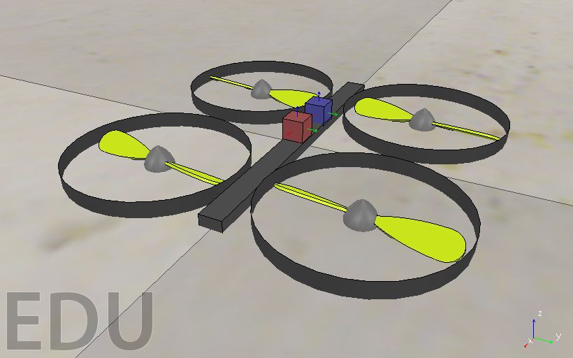
Figure 7: Quadcopter in V-rep simulator

V Results

Having designed the structure and set up an optimizer, we simulated the network using Python programming and PyTorch library. Additionally, V-rep Coppeliasim has been set to perform as a real environment. In this framework, the model of the quadcopter is completely unknown, and only the inputs and outputs of the system were used continuously. We considered certain scenarios to verify and challenge the proposed method.

V-A Squared path in a constant height

To begin with, a squared path in a constant height was chosen as a scenario for tracking. According to Figs. 11 and 11, at the beginning of the mission, the variance ($\sigma$) of choosing gains is high, and the agent tries to choose different actions to improve identification. Therefore, the rates of change of gains are high, and after a while, they decrease slightly until converging to a constant number. These figures indicate that the proposed method can efficiently control the attitude of the Quadcopter for a simple tracking scenario.

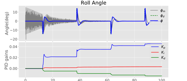
Figure 8: control of Roll ($\phi$) angle in the given scenario. The angle converges to zero, resulting in a good performance of controller.

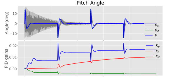
Figure 9: control of Pitch ($\theta$) angle in the given scenario. The angle converges to zero, resulting in a good performance of controller

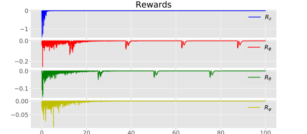
Figure 10: Received rewards of each agent during the mission

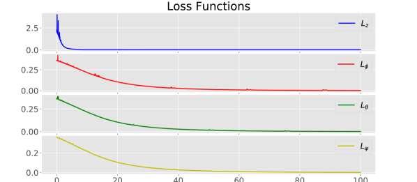
Figure 11: changes of the loss functions of each agent’s net during the mission

When the rewards (shown in Fig. 11) and the loss functions (shown in Fig. 11) of each agent increase over time to reach the optimal point, it emphasizes the fact that the network weights have been optimized, resulting in well-trained networks. Since the weights of the networks are trained in an online manner, this method is fast and can be used in real-world robots.

Tunning PID gains for the first scenario, the attitude control (Euler angles) could track the desired angles. When the attitude control is decent, position control can be attained simply (Fig. 12).

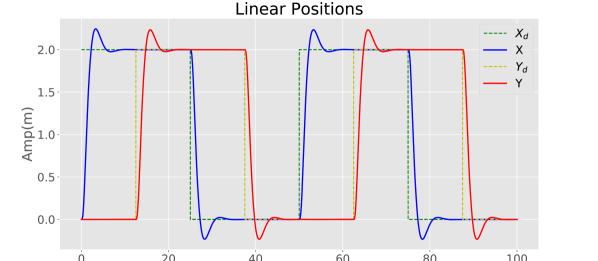
Figure 12: X and Y position tracking in squared tracking path

V-B Mass uncertainty

In the next step, we changed the total mass of the Quadcopter (Fig. 13) with respect to time to execute parameter uncertainty and challenge the efficiency of the network. The mass of the system changes significantly after a short period of time. When the system mass increases, the altitude of the system changes, which indicates that the corresponding controller should adapt itself to these changes. According to Fig. 13, the controller is able to compensate for the error of the system accordingly. Compared to traditional PID, it is obvious that the performance of the proposed controller is better when confronting mass uncertainty. Moreover, if we add more mass, the traditional PID method will not respond well because its gains have been designed for a system with a different mass. On the other hand, the proposed method can change the gains simultaneously, thereby preventing the error from getting bigger. As a result, this method is not only online but also adaptable to changes.

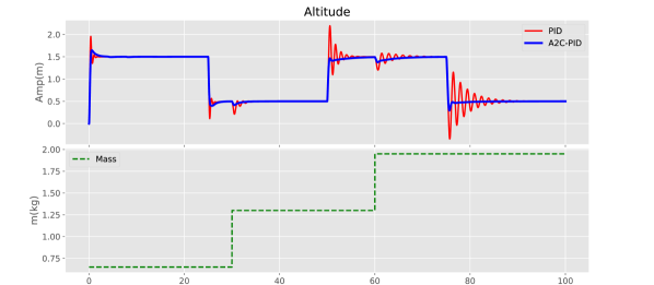
Figure 13: comparison between the response of proposed method versus PID controller in altitude control. The green line shows the changes of the total mass of the quadcopter

As a more complex scenario, we designed a helical path for the Quadcopter to ensure that the control system works well. When an underactuated robot like a Quadrotor can track desired positions in different directions, we can conclude that the attitude control of the system has been achieved successfully because the latter one is in the inner loop of the system and is a priority for the former one. Fig. 14 shows that the robot tracks the path appropriately, and the error is converging to zero. When position tracking is good, the attitude control is also fine.

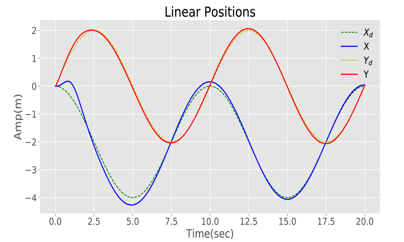
Figure 14: X and Y position tracking in helical tracking path

V-C Disturbance rejection

To challenge the performance of our method, we investigateed the impact of wind gust disturbance on attitude. Guass-Markov equations [19] are adopted, as indicated in the following equations:

$$\dot{d}=-\frac{1}{\tau_{s}}d+\rho B_{w}q_{w}$$ (17)

Eq. 17 is known as a ”shaping filter” for the wind gusts, where $q_{w}$ is an independent constant with zero mean, $\tau_{s}=0.3$ is the correlation time of the wind, $B_{w}$ is the turbulence input identity matrix, and $\rho=0.5$ is the scalar weighting factor. Eq. 17 was solved using the ODE45 method alongside Eq. 1, and Fig. 18 indicates the recorded disturbances during the mission with initial conditions set to zero. The size of each disturbance is sufficient to affect the performance of every controller.

TABLE I: Comparison of RMSE

Attitude (deg)	PID	A2CPID
roll($\phi$)	4.49	1.20
pitch($\theta$)	3.85	1.83
yaw($\psi$)	2.5	0.35

However, the proposed controller proves its robustness against disturbance in all attitude angles compared to conventional PID controller. After a time period, PID controller cannot compensate the increased error because the integrator gain is constant, whereas the proposed method can change this gain in an adaptive manner. In fact, this controller learns how to change gains using error, error rate, control input, and previous states.

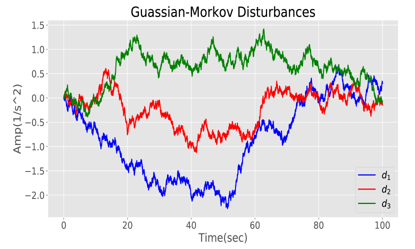
Figure 15: Guassian-Markov disturbances. $d_{1},d_{2},d_{3}$ are correspondent to $\phi,\theta,\psi$ and added to these angles respectively.

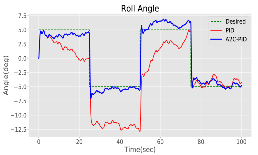
Figure 16: Tracking desired Roll ($\phi$) angle using proposed method and PID controller

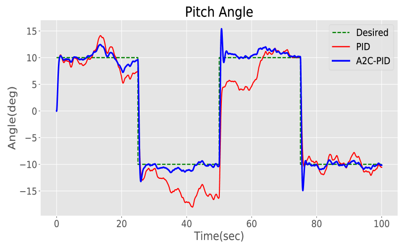
Figure 17: Tracking desired Pitch ($\theta$) angle using proposed method and PID controller

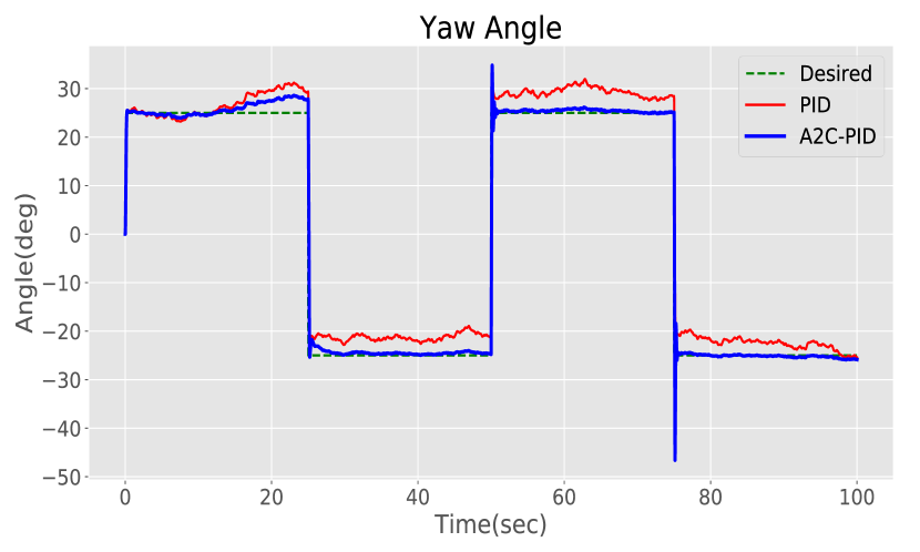
Figure 18: comparison between the performance of propsed method versus conventional PID method for cantrolling Yaw ($\psi$) angle

To compare the performance of the proposed method and conventional PID controller, Root Mean Square Error (RMSE) of each angle has been computed for both controllers and the results are shown in Table I.

VI conclusion

In this research, a novel self-tuning PID control has been proposed using a hybrid neural structure based on the actor-critic method. The proposed method is able to tune PID gains and identify states in an online manner. Not only does this method have a straightforward structure, but it is also applicable to real SISO systems. We have taken advantage of NNs and the Adam optimizer in this work, the latter of which is fast and reliable. Results showed that the control algorithm is able to track complex paths even with randomly initialized weights. Using this method, altitude control was achieved with mass uncertainty, and the response was good when confronting wind gust disturbances on attitude control. We have shown that the proposed method has far better results compared to the conventional PID method.

VII Acknowledgment

This research has proposed as the result of author’s master’s thesis and without any sponsorship.

References

- [1] J. Kim, S. A. Gadsden, and S. A. Wilkerson, “A comprehensive survey of control strategies for autonomous quadrotors,” Canadian Journal of Electrical and Computer Engineering, vol. 43, no. 1, pp. 3–16, 2019.
- [2] A. Zulu and S. John, “A review of control algorithms for autonomous quadrotors,” arXiv preprint arXiv:1602.02622, 2016.
- [3] T.-h. Pan and S.-y. Li, “Adaptive pid control for nonlinear systems based on lazy learning,” Control Theory & Applications, vol. 10, p. 029, 2009.
- [4] J. Yang, Z. Cai, Q. Lin, and Y. Wang, “Self-tuning pid control design for quadrotor uav based on adaptive pole placement control,” in 2013 Chinese Automation Congress, pp. 233–237, IEEE, 2013.
- [5] A. Goel, A. M. Salim, A. Ansari, S. Ravela, and D. Bernstein, “Adaptive digital pid control of a quadcopter with unknown dynamics,” arXiv preprint arXiv:2006.00416, 2020.
- [6] R. Hernández-Alvarado, L. G. García-Valdovinos, T. Salgado-Jiménez, A. Gómez-Espinosa, and F. Fonseca-Navarro, “Neural network-based self-tuning pid control for underwater vehicles,” Sensors, vol. 16, no. 9, p. 1429, 2016.
- [7] S. Bari, S. S. Z. Hamdani, H. U. Khan, M. ur Rehman, and H. Khan, “Artificial neural network based self-tuned pid controller for flight control of quadcopter,” in 2019 International Conference on Engineering and Emerging Technologies (ICEET), pp. 1–5, IEEE, 2019.
- [8] D. Park, T.-L. Le, N. V. Quynh, N. K. Long, and S. K. Hong, “Online tuning of pid controller using a multilayer fuzzy neural network design for quadcopter attitude tracking control,” Frontiers in Neurorobotics, p. 118, 2021.
- [9] O. I. Abiodun, A. Jantan, A. E. Omolara, K. V. Dada, N. A. Mohamed, and H. Arshad, “State-of-the-art in artificial neural network applications: A survey,” Heliyon, vol. 4, no. 11, p. e00938, 2018.
- [10] I. Carlucho, M. De Paula, S. A. Villar, and G. G. Acosta, “Incremental q-learning strategy for adaptive pid control of mobile robots,” Expert Systems with Applications, vol. 80, pp. 183–199, 2017.
- [11] Q. Shi, H.-K. Lam, B. Xiao, and S.-H. Tsai, “Adaptive pid controller based on q-learning algorithm,” CAAI Transactions on Intelligence Technology, vol. 3, no. 4, pp. 235–244, 2018.
- [12] Z. Guan and T. Yamamoto, “Design of a reinforcement learning pid controller,” IEEJ Transactions on Electrical and Electronic Engineering, vol. 16, no. 10, pp. 1354–1360, 2021.
- [13] N. P. Lawrence, M. G. Forbes, P. D. Loewen, D. G. McClement, J. U. Backström, and R. B. Gopaluni, “Deep reinforcement learning with shallow controllers: An experimental application to pid tuning,” Control Engineering Practice, vol. 121, p. 105046, 2022.
- [14] J. Yang, D. Chu, W. Peng, C. Sun, Z. Deng, L. Lu, and C. Wu, “A learning control method of automated vehicle platoon at straight path with ddpg-based pid,” Electronics, vol. 10, no. 21, p. 2580, 2021.
- [15] Q. Sun, C. Du, Y. Duan, H. Ren, and H. Li, “Design and application of adaptive pid controller based on asynchronous advantage actor–critic learning method,” Wireless Networks, vol. 27, no. 5, pp. 3537–3547, 2021.
- [16] D. P. Kingma and J. Ba, “Adam: A method for stochastic optimization,” arXiv preprint arXiv:1412.6980, 2014.
- [17] V. K. Tripathi, L. Behera, and N. Verma, “Design of sliding mode and backstepping controllers for a quadcopter,” in 2015 39th national systems conference (NSC), pp. 1–6, IEEE, 2015.
- [18] R. S. Sutton and A. G. Barto, Reinforcement learning: An introduction. MIT press, 2018.
- [19] L. Ding, Q. He, C. Wang, and R. Qi, “Disturbance rejection attitude control for a quadrotor: Theory and experiment,” International Journal of Aerospace Engineering, vol. 2021, 2021.