Does regional variation in wage levels identify the effects of a national minimum wage?

Abstract

This paper examines the identification assumptions underlying two types of estimators of the causal effects of minimum wages based on regional variation in wage levels: the "effective minimum wage" and the "fraction affected/gap" designs. For the effective minimum wage design, I show that the identification assumptions emphasized by Lee (1999) are crucial for unbiased estimation but difficult to satisfy in empirical applications for reasons arising from economic theory. For the fraction affected design at the region level, I show that economic factors such as a common trend in the dispersion of worker productivity or regional convergence in GDP per capita may lead to violations of the “parallel trends” identifying assumption. The paper suggests ways to increase the likelihood of detecting those issues when implementing checks for parallel pre-trends. I also show that this design may be subject to biases arising from the misspecification of the treatment intensity variable, especially when the minimum wage strongly affects employment and wages.

1 Introduction

One approach to measuring the effects of minimum wage regulations involves leveraging variation in wage levels across different regions within a country. For instance, the influence of the US federal minimum wage is more pronounced in states like Mississippi or Arkansas than in Texas or Georgia due to the higher median wages in the latter states. Thus, one can use wage distributions to construct treatment intensity measures for a “differences-in-differences” analysis. Classic applications using cross-state variation from the US are Card (1992), who introduced the “fraction affected” design, and Lee (1999), who introduced the “effective minimum wage” design. This strategy is particularly convenient in countries with little or no spatial variation in minimum wage laws. Examples of such applications published by leading economic journals include Mexico (Bosch and Manacorda, 2010), South Africa (Dinkelman and Ranchhod, 2012), Germany (Dustmann et al., 2021), the US in the 1960s and 1970s (Bailey, DiNardo and Stuart, 2021), and Brazil (Engbom and Moser, 2022).

This paper examines the identification assumptions underlying those econometric approaches. Specifically, it uses a combination of economic theory and simulation exercises to investigate whether fraction affected and effective minimum wage designs can accurately capture the causal effects of the minimum wage on employment and wages, using a range of economic models as data-generating processes.

For the effective minimum wage design, I show that two identification assumptions emphasized by Lee (1999) are crucial for unbiased estimation of causal effects but challenging to satisfy in typical applications. The first assumption is that the effective minimum wage should be constructed as the gap between the actual minimum wage and a good proxy for the centrality of the latent log wage distribution—that is, the distribution of log wages that would prevail with no minimum wage in place. Practitioners typically use the observed median log wage as that proxy. I show that this choice generally introduces correlated measurement error that can cause economically relevant biases. The second assumption is that overall wage levels should be uncorrelated with the dispersion of latent log wages across regions. This assumption may be violated if, for example, regions differ in the share of skilled workers, and there is more latent wage dispersion for skilled workers (Lemieux, 2006). I show that even small correlations, no larger than those observed in between-state data for the US, can introduce large biases.

I discuss the effectiveness of potential solutions to those problems with the effective minimum wage design. Those include testing for spillovers in the upper tail as a diagnostics tool, using higher quantiles of the wage distribution to construct the effective minimum wage, changing the set of fixed effects or trends included in the regression, or employing instrumental variables approaches in the style of Autor, Manning and Smith (2016). The general message is that the estimator is most likely to be successful when the econometrician can precisely point out the source of variation that is acting as the exogenous shifter of the effective minimum wage in a given context, taking into account context-specific knowledge and the set of fixed effects and controls used in the design.

Next, I discuss fraction affected and gap designs implemented at the regional level. The key identification assumption is transparent in those designs: in a counterfactual scenario without an increase in the national minimum wage, trends in outcomes would be orthogonal to the treatment intensity variable used, conditional on the controls and fixed effects used in the design. My analysis points to three potential issues practitioners should be aware of. First, I show that structural factors that may seem unproblematic, such as a common trend in the dispersion of latent log wages affecting all regions in the same way (due, e.g., to skill-biased technical change), may cause violations of the parallel trends assumption. Second, the design is subject to bias from regression to the mean in regional wage statistics, originating from sampling variation when constructing those statistics and from region-specific productivity shocks. Third, the design is sensitive to the functional form chosen for the treatment intensity variable, with misspecification biases being more significant when the minimum wage strongly affects employment and wages.

I also discuss possible diagnostics and solutions to those issues. I show that tests for differential pre-trends may effectively detect the first two issues when the data includes a “pre-treatment” period without significant changes in minimum wage laws. However, the econometrician needs to be careful in implementing the test—specifically, the treatment intensity variable (fraction affected or gap) should be constructed using a single pre-treatment year. On the other hand, controlling for region-specific trends may not be warranted if regression to the mean is quantitatively significant. For the misspecification issue, I show that using a binary measure of treatment intensity, loosely inspired by the work of Callaway, Goodman-Bacon and Sant’Anna (2021), does not help; it can make misspecification biases even more significant.

This paper contributes to the growing literature that points out econometric challenges associated with difference-in-differences designs in general and specifically regarding minimum wages. Sorkin (2015) and Vogel (2023) discuss problems arising from the fact that minimum wage effects on wages and employment may not materialize instantly, leading standard reduced-form estimators to mismeasure the long-run effects of minimum wage regulations. Autor, Manning and Smith (2016) highlight issues with the effective minimum wage design in the presence of measurement error. de Chaisemartin and D’Haultfœuille (2020) raise concerns regarding difference-in-differences designs with heterogeneous treatment effects and non-uniform timing of treatment that are relevant to the effective minimum wage design. Callaway, Goodman-Bacon and Sant’Anna (2021) explore identification challenges when the treatment variable in a difference-in-differences design is continuous, as is the case with all estimators examined in this paper (see also Roth et al., 2023, for a comprehensive review of recent advances in the econometrics of difference-in-differences designs). The issues discussed in this paper differ from and complement those addressed in the studies above.

The paper is structured as follows. Section 2 introduces the setup and defines the causal effects of interest. Sections 3 and 4 analyze the issues and potential solutions for the effective minimum wage and the fraction affected estimators, respectively. In Section 5, I show that simulation results shown in Sections 3 and 4 are not particular to the economic model used as the data-generating process. The final section concludes with recommendations for researchers interested in measuring the effects of national minimum wage changes in contexts without state variation in minimum wage laws.

2 Setup

I consider two-period data generating processes of the following form:

$$\bm{y}_{r,t}=f\left(mw_{t},\bm{\theta}_{r,t}\right)$$ (1)

where $r\in\{1,\dots,R\}$ denotes region, $t\in\{0,1\}$ denotes time, $\bm{y}_{r,t}$ is a vector of equilibrium outcomes (such as employment to population ratio or quantiles of the log wage distribution), $mw_{t}$ denotes the logarithm of the national minimum wage, $\bm{\theta}_{r,t}$ is a vector of region-time-specific parameters, and $f$ is a function that depends on the particular economic model (to be described later in the paper). Minimum wage levels are different between periods. Without loss of generality, I assume henceforth that $mw_{1}>mw_{0}$.

Equation (1) is fairly general, but it imposes important constraints that limit the scope of my analysis. First, because equilibrium outcomes in one region cannot affect outcomes in another, this model cannot be used to study econometric issues such as minimum-wage-induced migration or capital mobility. Second, the restriction to two periods means that I do not address econometric problems arising from the combination of treatment effect heterogeneity and differential timing of treatment assignment (see de Chaisemartin and D’Haultfœuille, 2020, for a discussion of this issue). Third, I also do not discuss the econometric difficulties associated with distinguishing between short- and long-run minimum wage effects (Sorkin, 2015; Hurst et al., 2022; Vogel, 2023). Fourth, the model does not include measurement error in observable outcomes, which may itself be a source of bias (Autor, Manning and Smith, 2016). Thus, this paper does not aim at providing a comprehensive account of econometric issues affecting minimum wage designs; instead, the contribution is pointing out some previously undocumented concerns.

The motivation for my study are papers that estimate the aggregate effects of a national minimum wage, like the ones cited in the beginning of the introduction. Given this purpose and the data-generating process described above, there are two natural ways to define the ceteris paribus causal effects to be identified:

$$\bm{ATE}_{0} =\frac{1}{R}\sum_{r}f\left(mw_{1},\theta_{r,0}\right)-f\left(mw_{0},\theta_{r,0}\right)$$

$$=\frac{1}{R}\sum_{r}f\left(mw_{1},\theta_{r,0}\right)-\bm{y}_{r,0}$$

$$\bm{ATE}_{1} =\frac{1}{R}\sum_{r}f\left(mw_{1},\theta_{r,1}\right)-f\left(mw_{0},\theta_{r,1}\right)$$

$$=\frac{1}{R}\sum_{r}\bm{y}_{r,1}-f\left(mw_{0},\theta_{r,1}\right)$$

The first considers a counterfactual where the minimum wage is increased to the level valid in period 1, keeping other characteristics constant at their $t=0$ levels. The other compares the outcomes as of $t=1$ to a counterfactual scenario where the minimum wage remained at the $t=0$ level. The two definitions are identical if the minimum wage is the only time-varying component of the model, and are equal in expectation if the parameters $\bm{\theta}_{r,t}$ have the same distribution across regions in both periods. This is true for some of the models I study, but not all. To keep the analysis as simple as possible, I use the average of these two definitions as the “true” causal effects to be recovered by the econometric designs:

$$\bm{ATE}=\frac{\bm{ATE}_{0}+\bm{ATE}_{1}}{2}$$

which gives equal weight to all observations in the data, and is thus closely related to the usual definition of average treatment effects in potential outcomes models.

All exercises in the paper impose an additional restriction on the data-generating process: there are no trends in overall wage levels. If the minimum wage change is simultaneous with an unobserved shock to total factor productivity (TFP), it is impossible to identify the average effects of the minimum wage change using the designs studied in this paper without imposing further assumptions. To abstract from this well-known “missing intercept” issue, I rule out such common TFP shocks (though I explore idiosyncratic, mean-zero TFP shocks). In practice, econometricians should in general interpret estimates coming from these regressions as the impact of the minimum wage net of these common TFP shocks.

3 The effective minimum wage design

3.1 Definition

Let $w_{q,r,t}$ denote quantile $q$ of the log wage distribution in region $r$ at time $t$. Then, define the log effective minimum wage as $mw_{t}-w_{0.5,r,t}$: the minimum wage relative to the median wage in region $r$ at time $t$. The effect of the minimum wage on the shape of the wage distribution is recovered by running separate regressions for different quantiles $q$ of the wage distribution, using the following functional form:

$$w_{q,r,t}-w_{0.5,r,t}=\alpha_{q,r}+\delta_{q,t}+\beta_{q}\left[mw_{t}-w_{0.5,r,t}\right]\\ +\gamma_{q}\left[mw_{t}-w_{0.5,r,t}\right]^{2}+\epsilon_{q,r,t}$$ (2)

which include region and time fixed effects, and where the effective minimum wage is allowed to have nonlinear effects on the outcomes. This specification is not the only one possible; alternative specifications will be discussed below.

To calculate the predicted treatment effects in each region $r$, I multiply the changes in the effective minimum wage (and its square) by the estimated $\hat{\beta}$ and $\hat{\gamma}$ parameters. Those products are then added up and averaged across regions, yielding the estimated average treatment effects of the national minimum wage increase following the definition from Section 2. As mentioned at the end of the previous section, if there are other structural factors generating a common trend in median wages, then this approach measures the combined effects of the minimum wage and that common trend.

The effective minimum wage design has been also used to estimate employment effects; Engbom and Moser (2022) is one example. In this case, the model is identical to Equation (2), except that the left-hand side contains the employment to population ratio.

This regression was first introduced by Lee (1999). In order to discuss its identifying assumptions, it is useful to introduce some of his notation. Suppose that each region has a latent distribution of log wage in each period—that is, the distribution of log wages that would prevail with no minimum wage regulation in place. Assume further that the cumulative distribution function for those latent log wages have the form:

$$F_{t}\left(\frac{w-\mu_{r,t}}{\sigma_{r,t}}\right)$$

where $\mu_{r,t}$ and $\sigma_{r,t}$ are the centrality and dispersion parameters, respectively.

Using this notation, Lee (1999) emphasizes two identification assumptions. First, the “deflator” used to construct the effective minimum wage—that is, the median wage $w_{0.5,r,t}$ in Equation (2)—should provide a good approximation for the centrality parameter $\mu_{r,t}$. Second, the location and dispersion parameters should be uncorrelated across regions conditional on $t$. When employment is the outcome of interest, one must also assume that “latent employment”—the one that would be observed in the absence of a minimum wage—is uncorrelated with location parameters, conditional on the fixed effects included in the regression.

The central message of my analysis below is that those assumptions are essential, but unlikely to hold in practice for economic reasons. Later, I will also show that the issues are less severe in contexts with regional variation in the minimum wage, and in those contexts, the instrumental variables estimator of Autor, Manning and Smith (2016) is preferable even if one disregards measurement error issues.

3.2 Issue #1: Imperfect measurement of latent centrality

The effective minimum wage design is predicated upon minimum wage effects being stronger where it bites more into the latent wage distribution. Following that logic, the econometrician would like to $mw_{t}-\mu_{r,t}$ as the key regressor. But because $\mu_{r,t}$ is not observed, $mw_{t}-w_{0.5,r,t}$ is used instead. Below, I argue that this issue is analogous to non-classic measurement error and may lead to point estimates that have the opposite sign compared to the true causal effects.

To build intuition on this problem, consider a model with two regions, $A$ and $B$. In period $t=0$, both regions have identical distributions of latent log wages. In period $t=1$, two things happen. First, the minimum wage increases by an amount $mw_{1}-mw_{0}=\Delta$. Second, the location parameter in region $B$ increases by the same amount: $\mu_{B,1}-\mu_{B,0}=\Delta$. Nothing else changes.

This example corresponds to “good” variation. Region $A$ is the “treatment group” while $B$ is the “control.” In $B$, the minimum wage binds as much in period $t=1$ as it did in $t=0$. Thus, we should expect no changes either in the effective minimum wage nor in outcomes such as quantile gaps or employment to population ratios. Even though the increase in the nominal minimum wage is the same everywhere, the comparison between those regions provides a valid quasi-experiment from which we can recover the causal effects of the minimum wage.

Now I describe how measurement error can introduce “bad” variation. The simplest example is to consider a scenario where, again, $A$ is affected by the increase in the national minimum wage. But now assume that location and dispersion parameters do not change over time, and that the “control” region $B$ is virtually unaffected by the minimum wage in both periods. That can be because location $\mu_{B}$ is significantly higher than $\mu_{A}$ in both periods. Alternatively, it may be that dispersion $\sigma_{B}$ is very small: wages are tightly concentrated around the median in region $B$, and thus a small or moderate minimum wage does not have any bite there.

What would one recover in this scenario using the effective minimum wage design? To make matters simple, consider a version of Equation (2) without the quadratic term. In a scenario with two regions, and with the inclusion of region and time fixed effects, the coefficient of interest is given by the double difference in outcomes divided by the double difference in the effective minimum wage:

$$\hat{\beta}= \frac{(y_{A,1}-y_{A,0})-(y_{B,1}-y_{B,0})}{\left[(mw_{1}-w_{0.5,A,1})-(mw_{0}-w_{0.5,A,0})\right]-\left[(mw_{1}-w_{0.5,B,1})-(mw_{0}-w_{0.5,B,0})\right]}$$

$$= \frac{(y_{A,1}-y_{A,0})-(y_{B,1}-y_{B,0})}{-\left[(w_{0.5,A,1}-w_{0.5,A,0})-(w_{0.5,B,1}-w_{0.5,B,0})\right]}$$

$$= -\frac{y_{A,1}-y_{A,0}}{w_{0.5,A,1}-w_{0.5,A,0}}$$

where $m_{r,t}$ is the outcome variable. The second line follows from eliminating common national minimum wage terms in the denominator. The third line follows from noting that the minimum wage has no effect on region $B$ in this model, and that the $B$ parameters are constant over time.

The numerator for this expression is the observed change in outcomes for region $A$, which in this model are caused by the minimum wage. The denominator is the change in the median wage in the same region. It would be positive and small if, for example, the minimum wage introduces some—but not much—truncation of the latent log wage. In this case, the estimated $\hat{\beta}$ would have the opposite sign compared to the true causal effects.

If the minimum wage causes a reduction of the median—for example, by increasing employment of low-wage workers in a context with monopsony power—then the estimated effects have the correct sign. However, the predicted change in outcome is likely to be much larger than the true causal effect, by a factor of $(mw_{1}-mw_{0})/(w_{0.5,A,1}-w_{0.5,A,0})$.

This problem is a form of measurement error in the sense that the effective minimum wage is an imperfect proxy for $mw_{t}-\mu_{r,t}$. It is not classical because minimum wage effects on the median wage should be correlated with minimum wage effects on other quantiles and on employment. And due to this correlation, the measurement error can plausibly cause an economically significant bias even if one has the strong prior that minimum wage effects on the median wage are close to negligible.

To investigate the potential magnitude of the bias in empirical applications, I perform simulation exercises with parameters calibrated based on state-level data from the US Current Population Survey. I assume that latent log wages are Normally distributed in every region. There is a “markdown” parameter $m\in[0,1]$ such that the latent distribution is truncated at $mw_{t}+\log m$, and censored at $mw_{t}$. That is: workers who would earn less than the minimum wage times the markdown become disemployed, and those with latent wages above that cutoff but below the minimum earn exactly the minimum wage. That model allows for spillovers arising from mechanical increases in wages even when disemployment effects are relatively small. Unless otherwise noted, all simulations have a markdown parameter of $m=0.7$.

Each region is described by a vector $[\mu_{r,0},\sigma_{r,0},\mu_{r,1},\sigma_{r,1}]$, drawn from a multivariate Normal distribution. The parameters for that multivariate Normal are calibrated based on state-level data from the US Current Population survey, based on the years of 1989 (corresponding to $t=0$) and 2004 (corresponding to $t=1$). Each particular simulation exercise makes different assumptions about that meta-distribution of parameters across regions, as explained below. In all exercises shown, the data contains 50 regions, and I show results averaged over 5,000 simulations. See Appendix A.1 for details.

Before showing the results, I make an important note. Since I ignore state-level minimum wage regulations in the US and only use two years, these results should not be interpreted as an evaluation of the effective minimum wage design in the US context. Rather, I use the US data to argue that the econometric issues I describe could be significant in contexts similar to the US with respect to the number of regions and how heterogeneous they are, but lacking variation coming from state-level minimum wages.

Table 1: Effective minimum wage design: good vs. bad variation

	Outcome
	Emp.	p10 - p50	p25 - p50	p90 - p50
Panel A: Regions differ only in location
True average causal effect	-0.010	0.019	0.006	-0.004
Effective min. wage	-0.010	0.019	0.006	-0.004
	(0.001)	(0.002)	(0.000)	(0.000)
Panel B: Regions differ in location and dispersion
True average causal effect	-0.010	0.020	0.006	-0.004
Effective min. wage	-0.007	0.033	0.014	-0.023
	(0.004)	(0.023)	(0.013)	(0.028)
Panel C: As above, but larger increase in min. wage
True average causal effect	-0.032	0.078	0.017	-0.012
Effective min. wage	-0.013	0.115	0.045	-0.079
	(0.015)	(0.040)	(0.023)	(0.053)
Panel D: St. dev. of dispersion is 50% larger
True average causal effect	-0.010	0.020	0.006	-0.004
Effective min. wage	-0.003	0.050	0.025	-0.047
	(0.006)	(0.033)	(0.020)	(0.041)

Notes: This table summarizes simulation results with 50 regions and two periods. The top row in each panel reports the average over 5,000 simulations of the true $ATE_{q}$ for different outcomes $q$, corresponding to different columns. The definition of $ATE_{q}$ is provided in Section 2. The second row shows estimated average treatment effects for each outcome based on the effective minimum wage regressions, averaged over the same 5,000 simulations. The third rows shows the average over simulatiosn of the corresponding standard errors, which in each simulation are clustered at the region level. The data-generating process includes both truncation and censoring effects of the minimum wage, as explained in the text. Each panel corresponds to a different assumptions on the data-generating process. In Panel A, regions differ only in the location parameter $\mu_{r,t}$, with a correlation between initial and final location of 0.89 as in US data. Panel B includes differences in the dispersion parameter $\sigma_{r,t}$, with a correlation between initial and final dispersion of 0.46. Panel C is like Panel B but with an increase of the log minimum wage of 0.4, instead of 0.2 as in other panels. Panel D increases the between-region standard deviation of the $\mu_{r,t}$ parameters between regions by 50%. See Appendix A.1 for details on the calibration of the model.

The first panel in Table 1 shows a case where all regions have the same dispersion parameters $\sigma_{r,t}=\sigma_{t}$, but differ in location parameters. The magnitude of between-state differences in the location parameter in each year, as well as the correlation between initial and final location within year, are calibrated to match the US data. This model corresponds to the ideal scenario with only “good” variation. Correspondingly, the estimator performs very well, with essentially no bias and very sharp confidence intervals.

Panel B introduces differences in dispersion parameters. It satisfies the structural assumptions emphasized by Lee (1999): distributions only differ in location and dispersion parameters, not shape, and the location and dispersion parameters have zero correlation with each other. Still, the estimator display economically meaningful biases. It arises because of the “bad” variation discussed above: the differences in dispersion, along with the fact that latent wages are not observable, introduce correlated measurement error. The biases are significant even though the minimum wage does not cause dramatic disemployment effects: the causal effect on the employment to population is of 1 percentage point, out of a baseline very close to 100%. Given the increase in the minimum wage of 20 log points, it corresponds to an employment elasticity with respect to the minimum wage of -0.05.

One may wonder whether a larger increase in the minimum wage would lead to more accurate estimates. On the contrary, Panel C shows that biases are larger in when the simulated increase in the federal minimum wage is of 40 log points. That is because, when the regression includes time and region fixed effects, the minimum wage in itself does not introduce good variation; that only comes from region-level shocks to location parameters. On the other hand, a larger minimum wage means that causal changes in the observed median wage are stronger, thus amplifying the bias caused by correlated measurement error.

Panel D highlights how this issue is intrinsically linked to differences in dispersion of latent log wages between states. Making those differences 50% larger in magnitude while keeping the other parameters constant is enough to essentially double the average bias in the regressions.

3.3 Issue #2: Correlation between location and dispersion parameters

The second assumption emphasized by Lee (1999) is independence between the location and dispersion parameters, $\mu_{r,t}$ and $\sigma_{r,t}$, conditional on $t$. For an intuition of why this assumption is essential for measuring spillover effects, consider again the “good variation” example from the previous subsection. In that example, region $A$ was “treated” by the minimum wage because its location parameters $\mu_{A,t}$ are constant over time, while region $B$ is the “control” because $\mu_{B,1}-\mu_{B,0}=mw_{1}-mw_{0}$. Now suppose that, along with the increase in location, the dispersion parameter also increases for region $B$. That would increase all quantile gaps $w_{q,B,t}-w_{0.5,B,t}$ in the control region. Thus, the comparison between changes in treatment versus control regions would not provide a valid estimate of the causal effects of the minimum wage anymore.

A correlation between location and dispersion parameters is also problematic if the outcome is employment. The reason is that changes in dispersion parameters can make the minimum wage bind more or less in some regions, causing independent effects on the median wage in the presence of a minimum wage. For example, rising dispersion can add more probability mass in the lower tail of the latent log wage distribution, increasing the amount of truncation and thus the mechanical effects of the minimum wage on the median wage. Thus, it may magnify the correlated measurement error issues previously discussed.

Below, I show through simulations that even mild contemporaneously correlation between location and dispersion parameters can introduce large biases in the effective minimum wage design. Next, I argue that there are plausible economic reasons why we should expect such correlations to occur.

Table 2: Correlation between location and dispersion parameters

	Outcome
	Emp.	p10 - p50	p25 - p50	p90 - p50
Panel A: No correlation between location and dispersion
True average causal effect	-0.010	0.020	0.006	-0.004
Effective min. wage	-0.007	0.033	0.014	-0.023
	(0.004)	(0.023)	(0.013)	(0.028)
Panel B: Contemporaneous correlation of 0.076
True average causal effect	-0.010	0.020	0.006	-0.004
Effective min. wage	-0.002	0.076	0.040	-0.075
	(0.004)	(0.021)	(0.012)	(0.026)
Panel C: Full correlation matrix in US data
True average causal effect	-0.010	0.019	0.006	-0.004
Effective min. wage	-0.014	-0.007	-0.010	0.029
	(0.004)	(0.022)	(0.013)	(0.027)

Notes: Each panel displays average results for 5,000 simulations, each with 50 regions and two periods, for different assumptions on the data-generating process (see the notes below Table 1 for an explanation of the structure of the table). Panel A is identical to Panel B in Table 1: regions differ in location ($\mu_{r,t}$) and dispersion ($\sigma_{r,t}$) parameters, but they orthogonal to each other. Panel B introduces a correlation of 0.076 between location and dispersion parameters within period, which is the correlation observed for US States in 1989. Panel C uses the full set of correlations between $[\mu_{r,0},\sigma_{r,0},\mu_{r,1},\sigma_{r,1}]$ observed in US data. See Appendix A.1 for details on the calibration of the model.

Panel A in Table 2 shows a baseline scenario where regions differ in dispersion parameters, but dispersion and correlation parameters are uncorrelated. Panel B introduces a within-period correlation of 0.076, which is the value I find in US data for 1989. That mild correlation is enough to bring the estimated employment effects to almost zero, and make estimated spillover effects much larger than the true ones. Note that this correlation does not significantly affect estimated standard errors; if anything, the estimates become more precise.

The US data also displays intertemporal correlations between location and dispersion. Panel C includes those correlations in the simulated model. The biases now go in the opposite direction, toward bigger estimated disemployment and smaller spillovers. That result shows that it may be difficult to predict the direction of the bias in empirical applications.

There are economic reasons why we should expect correlation between location and dispersion of latent log wages. One is the observation that, if workers are grouped by observable skill measures such as fine education-age-gender groups, higher skill is associated with more within-group inequality. This fact is discussed in detail by Lemieux (2006), who argues that much of the increase in inequality observed in the US from 1973 to 2003 is a compositional effect deriving from increased educational achievement. The same result has been found in other contexts, such as Brazil (Ferreira, Firpo and Messina, 2017). Then, if regions differ in workforce composition, the correlation we discussed above may follow. Furthermore, changes in workforce composition may also be heterogeneous between regions, leading to correlations in changes in addition to in levels.

Education is not the only economic factor that can introduce problems for the effective minimum wage design. Regional differences in endowments, leading to heterogeneity in industrial composition, may also generate correlation between location and dispersion parameters. That’s because industries—or clusters of connected industries that tend to co-locate—may differ in wage premiums and the breadth of occupations and skill levels used in production.

3.4 Fixed effects, trends, controls, and confounders

Lee (1999) uses a model without region fixed effects as his baseline specification and argues that the decision of whether to include them is not an obvious one. He writes: “… the reduced identifying variation resulting from eliminating the "permanent" state effects may magnify biases due to misspecification, in the same way biases stemming from measurement error in the independent variable are magnified when true variation in the independent variable is reduced.” Using the language introduced in Subsection 3.2, the estimator without region fixed effects has another source of “good” variation: within-period differences in the location parameters of latent log wage distributions (instead of simply differential shocks to location). That may significantly reduce the influence of “bad” variation coming from correlated measurement error in the centrality measure, reducing the amount of bias.

Still, it is easy to contemplate omitted variables that can be controlled for using region fixed effects. One example would be that unregistered employment, not visible in the data, is more relevant in low-wage areas, generating a spurious negative correlation between measured employment to population and the effective minimum wage. This is why I focused on the version with region fixed effects, as it is more popular in recent applications of that design.

Indeed, the specifications in papers such as Bosch and Manacorda (2010), Autor, Manning and Smith (2016), and Engbom and Moser (2022) go beyond region fixed effects, by including region-specific trends as well (with different trends for each outcome). These flexible trends may absorb region-specific supply and demand shocks that have an effect on the median wage and also on other outcomes, such as the shape of the distribution or employment. One example are changes in educational composition, which, as discussed in the previous subsection, may affect both the location and the dispersion of latent log wages. Another example are demand-side shocks such as “the China syndrome” (Autor, Dorn and Hanson, 2013), whose wage effects are not uniform over the distribution (being centered in the manufacturing sector) and whose employment effects may generate mechanical shifts in the median wage.

It is not clear, though, the extent to which region-specific trends reduce or amplify possible biases. The reason is analogous to Lee’s discussion of whether to include region fixed effects: by including the trends, the econometrician may be throwing the “good variation” out with the bathwater. Identification relies on the residual variation in the location parameter, after netting out all fixed effects, trends and controls used in the regression, to be orthogonal to the residual variation in dispersion parameters. Even if that holds, a smaller amount of “good” variation may amplify the measurement error issue from Subsection 3.2, amplifying the bias in the estimator.

Table 3: Effective minimum wage without time fixed effects

	Outcome
	Emp.	p10 - p50	p25 - p50	p90 - p50
Panel A: Regions differ only in location, stable distribution
True average causal effect	-0.010	0.019	0.006	-0.004
Effective min. wage	-0.010	0.020	0.006	-0.004
	(0.001)	(0.003)	(0.000)	(0.000)
Effective min. wage, no time FE	-0.010	0.019	0.006	-0.004
	(0.000)	(0.001)	(0.000)	(0.000)
Panel B: Regions differ in location and dispersion
True average causal effect	-0.010	0.020	0.006	-0.004
Effective min. wage	-0.007	0.034	0.015	-0.023
	(0.004)	(0.023)	(0.013)	(0.028)
Effective min. wage, no time FE	-0.007	0.052	0.024	-0.041
	(0.001)	(0.006)	(0.003)	(0.007)
Panel C: Full correlation matrix in US data
True average causal effect	-0.010	0.019	0.006	-0.004
Effective min. wage	-0.014	-0.006	-0.009	0.027
	(0.004)	(0.022)	(0.013)	(0.027)
Effective min. wage, no time FE	-0.007	0.048	0.022	-0.038
	(0.001)	(0.006)	(0.003)	(0.007)

Notes: Each panel displays average results for 5,000 simulations, each with 50 regions and two periods, for different assumptions on the data-generating process (see the notes below Table 1 for an explanation of the structure of the table). Panel A is similar to Panel A in Table 1 in that regions only differ in location parameters $\mu_{r,t}$, but makes the distribution of those parameters identical in both periods. Panel B has the same data-generating process as Panel B in Table 1, with uncorrelated location and dispersion parameters and small changes in the the distributions of those parameters over time. Panel C incorporates the full set of correlations between $[\mu_{r,0},\sigma_{r,0},\mu_{r,1},\sigma_{r,1}]$ observed in US data. See Appendix A.1 for details on the calibration of the model.

Based on this discussion, one may be tempted to drop the time fixed effects from the design. Lee (1999) explains why this choice may be unwise: it is only warranted if the econometrician believes the shape and average dispersion of latent log wages does not change over time. Thus, it is not a good assumption in the presence of secular trends in wages coming from technical change or international trade, for example.

Table 3 illustrates the sensitivity of that estimator to changes in the economic environment. Panel A only includes differences in location parameters, with the distribution of those parameters over regions stable over time. Panel B is the baseline scenario with differences in both location and dispersion, where average dispersion changes a bit over time (the most important being that the average $\sigma_{r,t}$ falls from 0.54 to 0.51). Panel C includes correlations between location and dispersion. The estimator without time fixed effects performs poorly whenever the model is not symmetric over time.

3.5 State-level minimum wages and instrumental variables

There is one case where adding region fixed effects, trends, and controls can still leave some “good” variation on the table: when there are changes in state-specific minimum wages. Then, by constructing the effective minimum wage measure using the prevailing minimum wage in the state—either the national or the state-specific, whatever is higher—, the econometrician can exploit that variation for identification. Still, the effective minimum wage estimator may remain biased, as it will use both the good variation coming from state-specific minimum wages and the bad variation induced by measurement error and the residual correlation between location and dispersion parameters.

One may then consider an instrumental variables estimator that isolates that source of good variation. One approach is to simply use the prevailing institutional minimum wage (and its square) as an instrument for the effective minimum wage (and its square). Autor, Manning and Smith (2016, henceforth AMS) implement that estimator for the US, arguing that it eliminates bias coming from measurement error in the median wage. In their specification, they include a third instrument: an interaction of the log minimum wage with the average median wage in each region. Because it uses observed median wages in its construction, this third instrument may be subject to some of the concerns discussed above.

Table 4: State-level minimum wages and instrumental variables approaches

	Outcome
	Emp.	p10 - p50	p25 - p50	p90 - p50
Panel A: No regional variation in minimum wage.
True average causal effect	-0.010	0.020	0.006	-0.004
Effective min. wage	-0.002	0.076	0.040	-0.075
	(0.004)	(0.021)	(0.012)	(0.026)
Panel B: 20% of regions with local min. wage
True average causal effect	-0.015	0.035	0.008	-0.005
Effective min. wage	-0.015	0.050	0.014	-0.018
	(0.003)	(0.009)	(0.005)	(0.012)
Two instruments	-0.016	0.036	0.009	-0.006
	(0.004)	(0.013)	(0.008)	(0.017)
Three instruments (AMS)	-0.017	0.041	0.008	-0.005
	(0.003)	(0.010)	(0.006)	(0.013)
Panel C: 40% of regions with local min. wage
True average causal effect	-0.020	0.053	0.011	-0.007
Effective min. wage	-0.019	0.059	0.015	-0.016
	(0.003)	(0.008)	(0.004)	(0.010)
Two instruments	-0.020	0.051	0.011	-0.007
	(0.003)	(0.009)	(0.005)	(0.011)
Three instruments (AMS)	-0.020	0.053	0.011	-0.007
	(0.003)	(0.008)	(0.005)	(0.010)

Notes: Each panel displays average results for 5,000 simulations, each with 50 regions and two periods, for different assumptions on the data-generating process (see the notes below Table 1 for an explanation of the structure of the table). Models in all panels are similar to those from Panel B in Table 2, where there is a small intra-temporal correlation between location ($\mu_{r,t}$) and dispersion ($\sigma_{r,t}$) parameters. Panels B and C introduce region-specific minimum wages. They differ in the share of regions with a local minimum wage higher than the national minimum wage. “Two instruments” corresponds to regressions that employ the nominal minimum wage and its square as instruments for the effective minimum wage and its square. “Three instruments (AMS)” adds a third instrument following Autor, Manning and Smith (2016). See Appendix A.2 for details.

Table 4 shows the results of simulations that include region-specific minimum wages and which implement those alternative instrumental variables estimators. As with the previous simulations, the parameters of the data-generating process are designed to replicate the US context; see Appendix A.2 for details. Panel A shows the baseline model, where there is small correlation between location and dispersion parameters (as in Table 2). Panels B and C add region-specific minimum wages that are higher than the national minimum wage. The difference between the panels is the share of regions with local minimum wages that are higher than the national minimum wage. In Panels B and C, I show results for not only the regular effective minimum wage design but also instrumental variables specifications, with either two or three instruments.

There are three takeaways from that table. First, the more variation coming from state-level minimum wages, the smaller the biases, even if one uses the ordinary least squares estimator. That can be noted by comparing the “Effective min. wage” rows across panels, noting that they become closer to the corresponding “Mean causal effect” rows. Still, some bias remains. Second, using instrumental variables approaches greatly reduces that bias. And third, biases are smallest when using the estimator with two, rather than three, instruments, though that comes at a cost in terms of precision.

One can thus view the issues discussed in this part of the paper as another motive for implementing instrumental variables regressions in the style of AMS, when the data includes regional-level variation in minimum wage laws. That is because, by not using the potentially endogenous variation coming from median wages, such estimators avoid the biases previously discussed. I also provide a reason to avoid using the “interaction” instrument if there is sufficient identifying variation in the minimum wage instruments alone.

3.6 Does using a higher quantile as the deflator help?

In some applications, the econometrician may have a strong prior that the minimum wage significantly impacts median wage, making it a poor measure of centrality. In those cases, they may consider using a higher quantile of the wage distribution to construct the effective minimum wage. For example, Bosch and Manacorda (2010) use quantile 0.7 as the deflator in a study of Mexico, and Engbom and Moser (2022) use quantile 0.9 when studying Brazil.

Table 5: Effective minimum wage using percentile 90 as the deflator

	Outcome
	Emp.	p10 - p90	p25 - p90	p50 - p90
Panel A: Regions differ only in location, stable distribution
True average causal effect	-0.010	0.023	0.009	0.000
Effective min. wage, p90	-0.010	0.024	0.009	0.000
	(0.001)	(0.003)	(0.001)	(0.000)
Panel B: Regions differ in location and dispersion
True average causal effect	-0.010	0.023	0.009	0.000
Effective min. wage, p90	0.009	0.219	0.176	0.000
	(0.003)	(0.026)	(0.021)	(0.000)
Panel C: Full correlation matrix in US data
True average causal effect	-0.010	0.023	0.009	0.000
Effective min. wage, p90	0.006	0.210	0.166	0.000
	(0.004)	(0.033)	(0.028)	(0.000)

Notes: This table has the same structure as Table 3, but reports regression results where the effective minimum wage is calculated based on percentile 90 of the observed log wage distribution, instead of the median log wage.

Lee (1999) argues that the “deflator” used to create the effective minimum wage should be the best approximation for centrality $\mu_{r,t}$. Otherwise, the regression may yield non-zero estimates even when the observed log wage distribution is identical to the latent wage distribution (that is, the minimum wage has no causal effects on wages). The discussion regarding correlated measurement error introduces another reason to be wary of choosing higher quantiles of the wage distribution. While is is true that those higher quantiles may be less affected by the minimum wage, the effects will still not be zero if the minimum wage has employment effects, positive or negative. In addition, higher quantiles may be much more affected by cross-region differences in the dispersion of latent log wages. Combining both issues, the biases may end up being larger than when using the median as the deflator.

Table 5 evaluates the performance of an estimator based on quantile 90 of the log wage distribution. I show three scenarios, identical to the ones from Table 3 (the one reporting the estimator without time fixed effects). When the data only includes shocks to the location parameter, and the distribution of those parameters is stable over time, that estimator works well. However, adding heterogeneity in dispersion parameters, along with small changes in the distributions of parameters over time, is enough to introduce dramatic biases, much larger than previously reported results in the paper. In unreported simulations, I tested that estimator in a wider range of scenarios, finding that it always underperforms relative to the estimator based on the median.

3.7 Is the standard diagnostic test effective?

Lee (1999) proposes estimating relative effects on “high” log wage quantiles $q>0.5$ to validate the model. The justification for that approach is that, in many applications (such as in the US), the econometrician may have a strong prior that the minimum wage should have minimal effects on the upper tail of the wage distribution. Autor, Manning and Smith (2016) use the same specification test to validate their instrumental variables implementation of the effective minimum wage design.

The econometrician must be aware, however, that such test is subject to both false positives and false negatives. False positives—detecting a problem where none exists—may arise because there are many plausible mechanisms that could lead to minimum wage spillovers that extend beyond the median wage. Engbom and Moser (2022) develop and estimate an on-the-job search model where minimum wages cause spillovers that extend far into the upper tail of the wage distribution, primarily due to worker reallocation from low- to high-wage firms. In Haanwinckel (2023), I argue that those spillovers can be compounded by endogenous changes in within-firm returns to skill in response to reallocation flows. Those channels may be quantitatively important even when net disemployment effects are small, as is the case in Engbom and Moser (2022). Thus, an econometrician with a strict rejection rule based on effects in the upper tail may reject a model that is valid.

There are two concerns regarding false negatives. One is that the estimator may be biased in the lower tail but not in the upper tail. This may happen if, for example, the negative upper-tail bias illustrated in Table 1 is combined with positive bias arising from measurement error, as discussed by Autor, Manning and Smith (2016). Second, even if such spurious upper tail spillovers are detected, the econometrician may still interpret those results as a negative, if they have the prior that such spillovers are economically plausible in the specific application, based on the theoretical arguments mentioned above. Thus, the upper tail test may not be an effective arbiter when different researchers disagree on the extent of spillovers in a particular scenario.

3.8 Taking stock

The core message of this discussion is that, to evaluate whether the effective minimum wage strategy is likely to be successful, the econometrician should have a clear sense of where the identifying variation is coming from. Exogenous changes in state-level minimum wages are the clearest example of such variation. Even when that variation is available, the effective minimum wage estimator might have some bias. Instrumental variables approaches such as that in Autor, Manning and Smith (2016) may be helpful.

If there is not much variation in state-level minimum wage laws, then does the variation in wage levels identify the effects of the national minimum wage? My analysis shows that this is only the case if, conditional on the fixed effects (or trends) used in the regression, differences in median wages come from an underlying structural factor that shifts the location of latent log wage distributions but has no independent effects on shape, dispersion, or employment. If the econometrician cannot think of what could be that structural factor in a particular application, then the effective minimum wage design may not be warranted.

The existence of a plausible structural shifter for location parameters that is orthogonal to dispersion parameters is not sufficient, however, for unbiased estimation. That’s because observed median wages are not a perfect proxy for centrality of the latent log wage distribution. The ideal scenario, then, is one where that plausible structural shifter is observable, such that the econometrician may directly exploit it in an instrumental variables approach.

4 Fraction Affected and Gap estimators

4.1 Definition

Now I study a difference-in-differences model with a time-invariant, continuous measure of treatment intensity based on the initial distribution of wages:

$$y_{o,r,t}=\alpha_{o,r}+\delta_{o,t}+\beta_{o}FA_{r}\cdot\bm{1}\{t=1\}+\epsilon_{o,r,t}$$ (3)

where the subscript $o$ indexes a specific equilibrium outcome, such that different $o$ correspond to separate regressions. The treatment intensity variable $FA_{r}$ is the “fraction affected,” that is, the share of workers in the initial period earning less than $mw_{1}$. The regressions include region and time fixed effects.

Given the linearity of this model, the estimated average treatment effect of the national minimum wage increase on outcome $o$ is given by the product of the average of $FA_{r}$ and the estimated $\hat{\beta}_{o}$ parameter.

The fraction affected design was first introduced by Card (1992), in an analysis of the 1990 increase in the federal minimum wage in the US. Card emphasizes that much of the identifying variation in his application comes from significant heterogeneity in the bindingness of state-level minimum wages in the preceding years. Since that original application, that estimator has been applied in other contexts with no regional variation in nominal minimum wages, such as the introduction of a federal minimum wage in Germany in 2015 (Ahlfeldt, Roth and Seidel, 2018; Fedorets and Shupe, 2021).

Identification comes from the comparison of trends for “more treated” versus “less treated” units, where the treatment intensity variable only uses information from the initial period. This design is thus fundamentally different from the effective minimum wage one, which, as discussed in the previous section, relies on idiosyncratic shocks to the location parameter of latent log wage distributions (when the regression includes both region and time fixed effects). The core identification assumption is standard for differences-in-differences designs: absent the increase in the national minimum wage, outcomes in treatment and control regions would evolve in a similar manner.

This design is ideal in scenarios where there is an increase in the minimum wage after at least a few years without adjustments. In those cases, the econometrician can use pre-treatment data to check for differential trends, which may provide support for the parallel trends identification assumption. I will discuss the effectiveness of the parallel trends assumption in detecting each of the issues I highlight in the next subsections.

I also study a closely related design based on the “Gap measure:”

$$y_{o,r,t}= \alpha^{Gap}_{o,r}+\delta^{Gap}_{o,t}+\beta^{Gap}_{o}Gap_{r}\cdot\bm{1}\{t=1\}+\epsilon^{Gap}_{o,r,t}$$

$$Gap_{r}= \frac{\sum_{i=1}^{I_{r}}\max\{\exp(mw_{1})-\exp(w_{i,0}),0\}}{\sum_{i=1}^{I_{r}}\exp(w_{i,0})}$$

where $i\in\{1,\dots,I_{r}\}$ indexes workers in the initial period and $w_{i,0}$ is their log wage in that period. That definition of treatment intensity was introduced in Card and Krueger (1994) in a firm-level econometric design. It has later been extended to region-level designs like the ones studied in this paper. Dustmann et al. (2021) provides an example, again in the context of Germany. It corresponds to the resulting relative increase in average wage in each region if all low-wage workers were to receive raises to comply with the new minimum.

4.2 Issue #1: Sensitivity to functional form assumptions

The fraction affected and gap designs are typically employed as model-agnostic approaches, in the sense that papers using those regressions do not take a strong stance on the underlying economic model of minimum wages. Still, they are based on a theoretical conjecture: treatment intensity is approximately proportional to a pre-determined sensitivity measure at the regional level. If the chosen functional form for that sensitivity measure is not correct, the conditional expectation function may be misspecified, in which case estimates of average treatment effects based on that estimator may be biased.

Table 6: Fraction Affected and Gap measures as imperfect proxies of treatment intensity

	Outcome
	Emp.	p10	p25	p50	p90
Panel A: Initial min. wage is small, $m=0.7$
True average causal effect	-0.006	0.016	0.008	0.004	0.002
Fraction affected	-0.008	0.020	0.010	0.005	0.003
	(0.000)	(0.002)	(0.001)	(0.002)	(0.002)
Gap measure	-0.006	0.015	0.007	0.004	0.002
	(0.000)	(0.001)	(0.001)	(0.001)	(0.001)
Panel B: Initial min. wage is small, $m=0.9$
True average causal effect	-0.018	0.043	0.022	0.012	0.006
Fraction affected	-0.019	0.038	0.022	0.013	0.006
	(0.000)	(0.001)	(0.001)	(0.002)	(0.002)
Gap measure	-0.015	0.029	0.017	0.010	0.005
	(0.000)	(0.002)	(0.001)	(0.001)	(0.001)
Panel C: Initial min. wage is large, $m=0.7$
True average causal effect	-0.042	0.162	0.049	0.028	0.013
Fraction affected	-0.053	0.153	0.063	0.036	0.018
	(0.001)	(0.021)	(0.005)	(0.002)	(0.002)
Gap measure	-0.037	0.101	0.044	0.025	0.013
	(0.001)	(0.017)	(0.003)	(0.002)	(0.002)
Panel D: Initial min. wage is large, $m=0.9$
True average causal effect	-0.079	0.126	0.084	0.053	0.027
Fraction affected	-0.073	0.071	0.067	0.052	0.030
	(0.002)	(0.003)	(0.002)	(0.002)	(0.002)
Gap measure	-0.052	0.050	0.048	0.037	0.021
	(0.002)	(0.003)	(0.002)	(0.002)	(0.002)

Notes: In all panels, the national minimum wage increases by 20 log points from the first period to the second. Regions differ only in the time-invariant location parameter $\mu_{r}\sim\mathcal{N}(0,0.2^{2})$. Each panel displays average results for 5,000 simulations, each with 50 regions. For each outcome, the numbers correspond to the mean true ATE across simulations, the mean estimates of causal effects based on the regressions listed on the left, and the average standard error associated with the estimates (in parentheses, clustered at the region level).

To investigate this possibility, I run simulations based on the same model used in the previous section: latent log wages are Normal in each region, and the minimum wage causes a combination of truncation and censoring effects depending on the markdown parameter $m$ (see Appendix A.1 for details). The simulations are designed to be “ideal” applications for the fraction affected and gap designs. First, the increase in the national minimum wage is the only time-varying factor in the model, preventing violations of the parallel trends assumption. Second, regions only differ in their time-invariant location parameter $\mu_{r}$. Thus, misspecification is coming solely from functional form assumptions, not from the fact that sensitivity to the minimum wage is a result of multi-dimensional heterogeneity and thus may be imperfectly captured by any unidimensional metric.

I simulate data under four specifications, encompassing different values of the markdown parameter $m$ (0.7 or 0.9) and different values for minimum wages. In all scenarios, the national log minimum wage increases by 0.2. But in Panels C and D, the initial minimum wage is higher, and because it bites more into the latent distribution, the employment and wage effects are more significant.

Table 6 shows that even in this ideal scenario, biases arising from functional form misspecification may be statistically and economic significant. In fact, the direction of the bias may change depending on the size of the markdown in the structural model. Even conditional on the estimator and data generating process, the bias can be toward zero for some outcomes and away from zero for others, showing that the misspecification of the treatment variable should not always be viewed as classic measurement error. The biases are larger when the minimum wage is more binding.

The measured employment and wage effects tend to smaller in magnitude when estimated with the Gap measure, given this particular data generating process. If one is interested in the ratio of employment effects to wage effects in the lower tail (proxying for the employment elasticity with respect to the worker’s wage), then the estimators are remarkably similar with each other across panels. But the estimated ratio is in general not equal to the true one.

One may wonder whether using a binary treatment intensity measure may help with misspecification issues. Callaway, Goodman-Bacon and Sant’Anna (2021) argue that, in difference-in-differences designs with continuous treatment variables, a binary design may be easier to interpret, if the control group in the binary design is composed of units which are not treated at all. But this is not the case for the data-generating processes studied here, since all regions may be affected by the national minimum wage.

In Appendix Table A3, I show that a binary definition of treatment suffers from stronger, not weaker, biases. I split regions into treatment or control groups based on whether the initial median wages are below a given threshold. The thresholds are chosen such that either half or 90% of the regions are in the treatment group. Consistent with the logic of Callaway, Goodman-Bacon and Sant’Anna (2021), biases are smaller when 90% of the sample are in the treatment group, since that makes the assumption that The predicted average treatment effects using that designed are substantially biased toward zero, consistent with the intuition that the binary classification introduces measurement error in the dependent variable.

4.3 Issue #2: Regression to the mean at the regional level

The fraction effected and gap measures are constructed based on extreme wage observations, in the sense that individual workers only contribute to those measures if their wages are below some threshold. Thus, these estimators may in principle be subject to bias emerging from regression to the mean. This is a well-known issue in the context of minimum wage studies, and most papers performing individual-level analysis at the firm or worker level discuss it. For example, in their worker-level analysis, Dustmann et al. (2021) use data from before the minimum wage was implemented to control for regression to the mean.

That issue is often ignored in regional-level studies. There are theoretical reasons why we regression to the mean is likely to be a much less serious concern with aggregate data. Assuming the data is a repeated cross-section, the individuals sampled in the “after” period are different from the ones sampled in the “before” period, and thus the individual-level concern does not mechanically translate into an aggregate one automatically. The sampling error in the measurement of the fraction affected may still generate return to the mean, since a region may have a high fraction affected because of an “unlucky” draw of workers in the survey. That concern becomes smaller with large sample sizes, but may not be negligible, especially if the statistics for most affected regions are calculated using small samples.

Time-varying structural factors that determine regional wages may also introduce reversion to the mean if they display autocorrelation. Caliendo et al. (2017) document that regional-level productivity shocks are quantitatively important in the United States. Gennaioli et al. (2014) collect time-series data on regional GDP for 83 countries and document within-country regional convergence. Their results mean that, in general, regions that have particularly low GDP per capita in a given period are likely to have stronger growth ex-post. Since these regional productivity shocks may affect both wages and employment, potential biases are not limited to regressions where wages are the dependent variable. That kind of regression to the mean is likely to be be more consequential for longer-run specifications.

Table 7: Sensitivity of the Gap design

	Outcome
	Emp.	p10	p25	p50	p90
Panel A: Only permanent differences in location
True average causal effect	-0.010	0.026	0.012	0.007	0.003
Gap measure	-0.009	0.027	0.011	0.006	0.003
	(0.000)	(0.003)	(0.001)	(0.001)	(0.001)
Panel B: Adding location shocks, stable distributions
True average causal effect	-0.010	0.026	0.012	0.007	0.003
Gap measure	-0.007	0.043	0.031	0.027	0.024
	(0.001)	(0.010)	(0.012)	(0.012)	(0.013)
Panel C: Adding dispersion differences and shocks, stable distributions
True average causal effect	-0.010	0.026	0.013	0.007	0.003
Gap measure	-0.007	0.052	0.034	0.024	0.008
	(0.002)	(0.012)	(0.012)	(0.012)	(0.018)
Panel D: Average dispersion falls over time
True average causal effect	-0.010	0.026	0.013	0.007	0.003
Gap measure	-0.004	0.046	0.032	0.023	0.009
	(0.002)	(0.013)	(0.013)	(0.013)	(0.019)

Notes: All panels illustrate scenarios where the only time-varying factor is an increase in the national minimum wage of 20 log points. Each panel displays average results for 5,000 simulations, each with 50 regions and two periods. For each outcome, the numbers correspond to the mean true ATE across simulations, the mean estimates of causal effects based on the regressions listed on the left, and the average standard error associated with the estimates (in parentheses, clustered at the region level). See the notes for Tables 1 and 2 for a description of Panels A and B.

The comparison between Panels A and B in Table A4 illustrates this issue in the context of the Normal-markdown model previously used in this paper. It reports results for the Gap design; Table A4 in Appendix B shows very similar results for the Fraction Affected design. In Panel A, regions only differ in a time-invariant location parameter $\mu_{r}$. Panel B introduces time-specific location parameters $\mu_{r,t}$, with the initial and final parameters for each region being jointly Normal with a correlation of 0.894 (which is the correlation between state-level mean log wages in the US for 1989 and 2004). As expected, the estimated wage effects become substantially more positive.

Panel C further to explore this issue by including time-varying heterogeneity in dispersion parameters $\sigma_{r,t}$ between regions. Those parameters are assumed to be independent of the location parameters, but have an autocorrelation of 0.456 between periods. That magnifies the positive bias in the lower tail, though it reduces it in the upper tail.

Fortunately, biases arising from regression to the mean can be detected with tests for differential pre-trends, if the context allows for such test. Appendix Table A5 illustrates this concept using a placebo exercise that parallels Table 7. The Gap measure is calculated as if the national minimum wage would increase by 0.2, but in fact there is no increase from period 0 to 1. That placebo exercise shows positive employment effects that have about the same size as the biases discussed above.

For the pre-trends test to work well in detecting that issue, the econometrician needs to be careful in how to define the treatment intensity variable. There are papers where the fraction affected or gap measures are constructed using all years before the increase in the minimum wage. For example, in their regional analysis, Dustmann et al. (2021) calculate the regional Gap measure for each year in the period before the new minimum wage, and then use the average for all of those years as the main regressor. Such definition is likely to reduce the amount of regression to the mean in the post-period, but does not eliminate it. More consequentially, it prevents the issue from being detected in the differential pre-trends test. Thus, it may be preferable to use a single pre-period year when creating the treatment intensity variables, at least for the purposes of checking for differential pre-trends.

Another implication of regression to the mean is that using region-specific linear trends to control for deviations of the parallel trends assumption may not be a valid strategy. The reason is that, in an “event study” graph, regression to the mean implies a V-shaped pattern with the bottom located in the year used to construct the treatment variable. Thus, if one were to extrapolate the pre-trends into the post-period and use it as the counterfactual, they would increase the bias in the estimated treatment effects, instead of attenuate it.

4.4 Issue #3: Trends in the dispersion of latent wages

Suppose that, in all regions, there is a change in the dispersion of latent log wages occurring at the same time as the increase in the national minimum wage. Since that shock is common across regions, one may expect that its influence will be captured by the time fixed effects included in the regressions. This subsection shows that this may not be the case when the minimum wage is not zero in the initial period.

Panel A: Fraction affected is larger at the top region

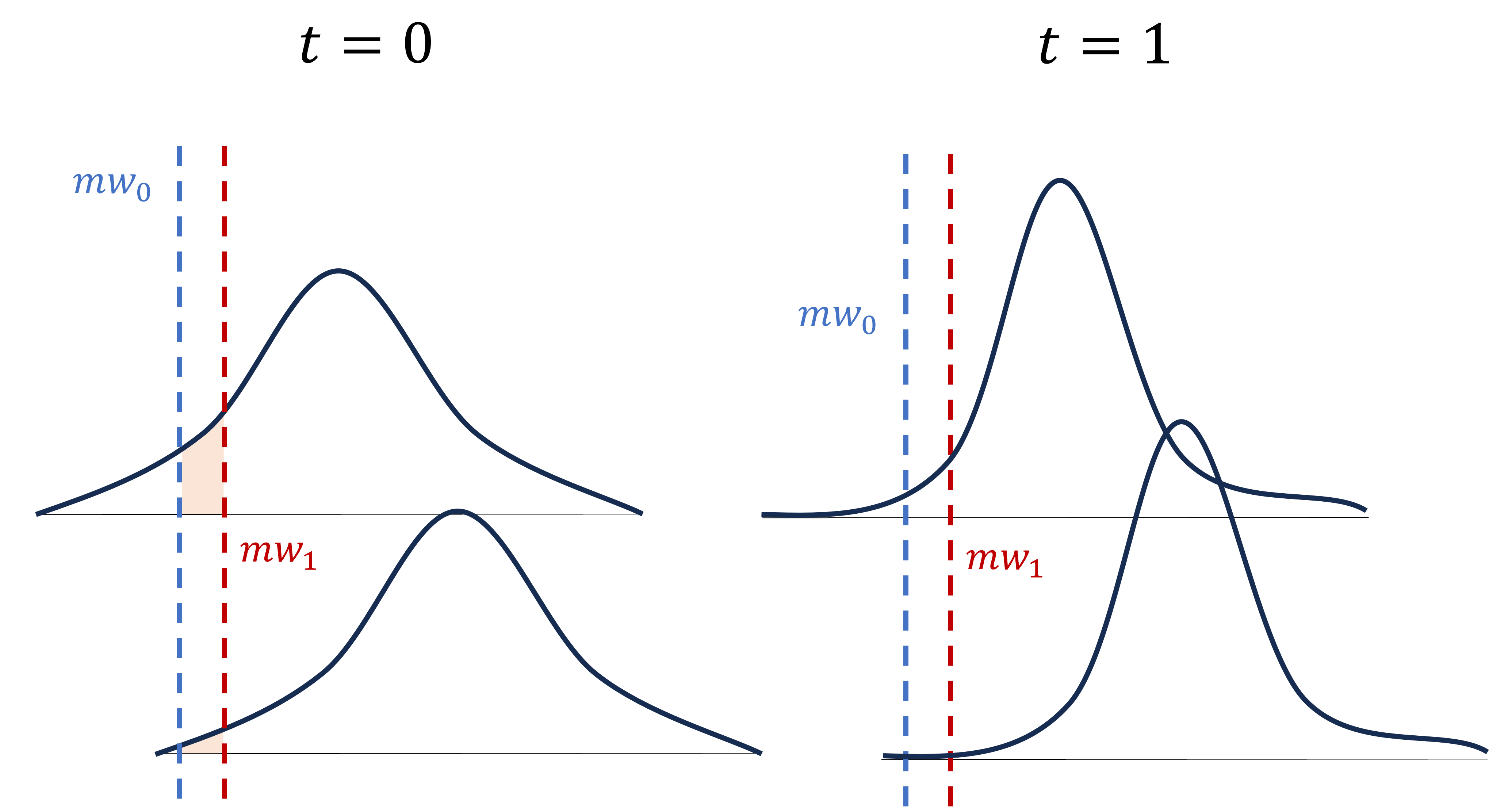
Panel B: Observed employment rises in the top region

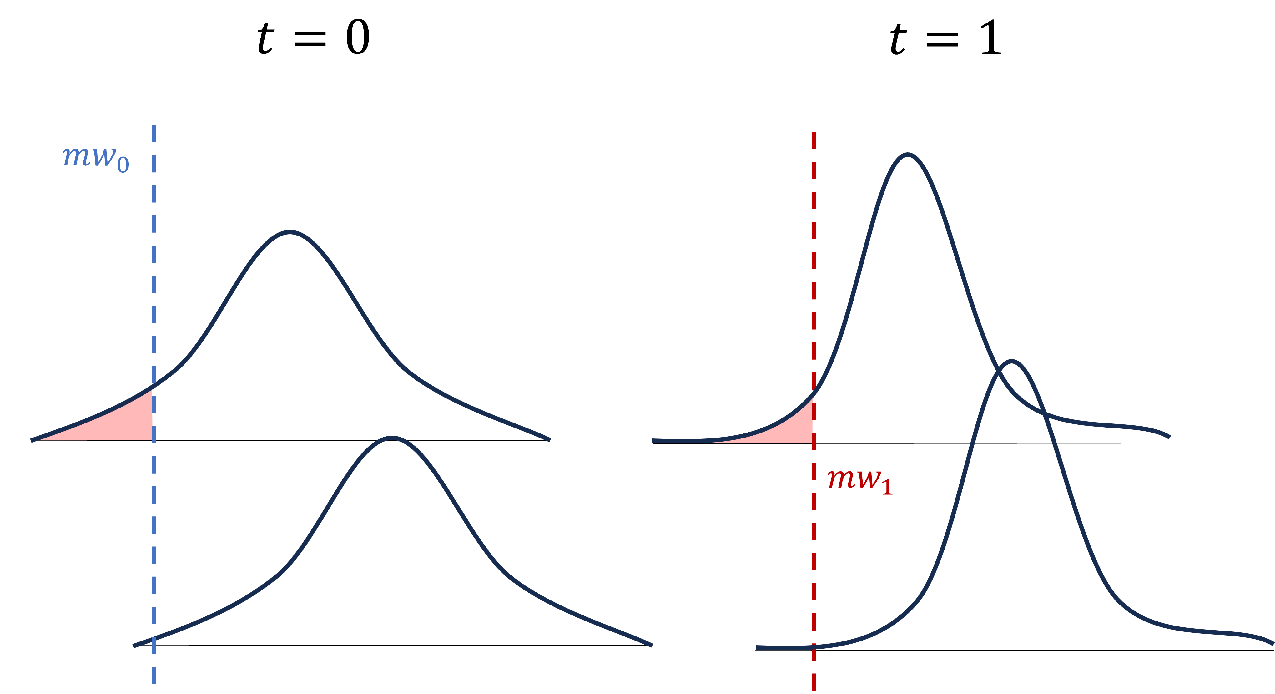
Figure 1: A truncation model with a secular decline in latent log wage dispersion

Consider the model illustrated in Figure 1. Regions differ in a location parameter $\mu_{r}$ that is constant over time. There is a common shape parameter $\sigma_{t}$ that decreases over time. Suppose that the minimum wage change is not that large, such that the new minimum is always to left of the peak of the latent log wage distribution. All else equal, regions with low $\mu_{r}$ a higher fraction affected and a higher causal effect of the minimum wage. But with the fall in $\sigma_{t}$, these regions may actually see a relative increase in employment. That is because as latent wages become more concentrated around the median, they may become less truncated. This effect may be negligible for regions with high $\mu_{r}$. As a result, the estimator may recover a positive relationship between the fraction affected and employment, despite the causal effects are negative for all observations in all periods.

The comparison between Panels C and D in Table 7 illustrates this issue. Panel C was discussed in the previous subsection: there are idiosyncratic shocks to both location and dispersion parameters, but the distributions of those parameters are stable over time. Panel D differs by imposing a small reduction in the average dispersion parameter $\sigma_{r,t}$, from 0.54 in $t=0$ to 0.51 in $t=1$. This small change is enough to reduce the measured employment effects by almost half, making them statistically different from the true causal effects on average.

If the trend in dispersion is a long-run phenomenon that has started before the minimum wage change, and that happens at a steady rate, then that bias can be detected in tests for differential pre-trends, as illustrated in the placebo tests shown in Appendix Table A5. The comments made in the previous subsection apply: for those tests to be most effective, the treatment intensity variable should be calculated based on a single year, instead of averaged over all pre-treatment years. In addition, one must be aware of the possibility that pre-trends look flat because they combine the effect of regression to the mean (discussed in the previous subsection) and other secular trends that have a stronger effect on treated regions. If this is recognized as a plausible concern in a given application, the econometrician may consider estimating a structural time-series model using pre-treatment data to quantify, and potentially correct for, the regression to the mean component.

4.5 Taking stock

I showed that the Fraction Affected and Gap designs explore a fundamentally different, and perhaps more transparent, source of variation compared to the effective minimum wage design. It relies strongly on the well-understood parallel trends assumption. Part of my contribution is showing that some factors that do not seem problematic, such as common trends in the dispersion of latent log wages, can imply violations of the parallel trends assumption. That makes it all the more important to report tests for differential pre-trends. Those tests are most effective when the treatment variable is constructed using only one pre-treatment period.

I also showed that, because those estimators are fundamentally reliant on the functional form used to construct the treatment variable, they are sensitive to model misspecification. Practitioners are encouraged to report predicted employment and wage effects using from multiple specifications. Still, it should be noted that the truth is not guaranteed to lie somewhere in between the Fraction Affected and Gap estimates; both may be biased in the same direction. This is especially likely when the minimum wage is more binding, in which case both estimators tend to under-estimate the negative employment effects and positive lower-tail wage effects caused by the minimum wage under the Normal-markdown model.

5 Robustness to alternative data generating processes

One may wonder whether the conclusions from the previous sections were sensitive to the data generating process used in the simulations. In this section, I show that the performance of the estimators is also limited under two alternative economic models: the canonical model of labor demand and the task-based monopsonistic model with firm heterogeneity from Haanwinckel (2023).

5.1 The canonical model of labor demand

Consider a competitive economy with two types of labor, low- or high-skill. Each worker is characterized not only by their type but also by their amount of efficiency units of labor. Wages are determined by marginal products of labor, which are determined by a representative production function with constant returns and constant elasticity of substitution. This is the basic setup in Katz and Murphy (1992).

Now consider the implications of a binding minimum wage. The representative firm will not employ workers whose productivity is below the minimum wage. Thus, one can think of this model as one where each worker has a latent log wage given by the sum of the log price of the efficiency unit of their type (low- or high-skill) and the log of their amount of efficiency units. The observed wage distribution is the truncated version of the latent one. See Appendix A.3 for details on the model.

The key difference compared to the model presented before is that the latent log wage distribution responds to the minimum wage. As the minimum wage causes more disemployment for low-skill workers, returns to skill are expected to fall. That generates wage spillovers for other low-skill workers and attenuates the negative disemployment effects.

Appendix Table A6 reports simulations that assess the effectiveness of the Fraction Affected and Gap designs using the Canonical model as the data-generating process. In those simulations, regions only differ in the initial share of workers that belong to the high-skill group, and the only time-varying factor is the minimum wage. In that sense, they parallel Table 6 above, illustrating ideal scenarios for the Fraction Affected and Gap designs. Also similarly to that previously discussed table, I report results for different model specifications, varying the bindingness of the initial minimum wage and the elasticity of substitution between low- and high-skill workers.

The are largely the same as those from Table 6. The predicted average causal effects estimated using those approaches do not always equal the true ones, and those misspecification biases are larger when the minimum wage is more binding.

Appendix Table A7 evaluates the effective minimum wage design using the same simulations. The baseline effective minimum wage specification, using both region and time fixed effects, displays severe biases. That is because the model does not include region-specific wage shocks, the key source of “good” variation in that design. For that reason, I also report estimates for the model without region fixed effects (the baseline specification in Lee, 1999), which exploit differences in wage levels (not changes). The model is almost ideal for that design in that there are no sources of “endogeneity” (like systematically lower latent employment levels in low-wage regions), and also in that the dispersion of efficiency units for both low- and high-skill workers are the same (which reduces the correlation between “location” and “dispersion” parameters of latent log wages). Even then, that model displays significant biases in some specifications.

5.2 A task-based, monopsonistic model with firm heterogeneity

Table 8: Quality of fit of the task-based, monopsonistic model

	Data		Model
	1998	2012	1998	2012	R2
Moments	(1)	(2)	(3)	(4)	(5)
Log wage gaps between educational groups
Secondary / less than secondary	0.498	0.168	0.486	0.15	0.77
Tertiary / secondary	0.965	1.038	0.995	0.932	0.131
Variances of log wages within educational groups
Less than secondary	0.41	0.241	0.387	0.225	0.575
Secondary	0.684	0.355	0.647	0.335	0.831
Tertiary	0.702	0.624	0.69	0.644	0.051
Two-way fixed effects decomposition
Variance establishment effects	0.116	0.056	0.117	0.057	0.652
Covariance worker, estab. effects	0.049	0.048	0.058	0.048	0.421
Formal employment rates by educational group
Less than secondary	0.266	0.337	0.266	0.336	0.951
Secondary	0.435	0.508	0.435	0.508	1.0
Tertiary	0.539	0.629	0.539	0.631	0.878
Minimum wage bindingness
Log min. wage - mean log wage	-1.418	-0.922	-1.418	-0.922	1.0
Share < log min. wage + 0.05	0.031	0.053	0.03	0.074	0.696
Share < log min. wage + 0.30	0.086	0.212	0.099	0.218	0.892

Notes: This table is adapted from Haanwinckel (2023). “Data” corresponds to statistics calculated at the microregion level using Brazilian data. “Model” corresponds to the model fit using that data as input. Columns (1) through (4) report averages for all regions for each of the two years, using region weights based on total formal employment. Column (5) reports the usual R2 metric $r^{2}_{e}=1-\left[\sum_{t=1}^{2}\sum_{r=1}^{151}s_{r}\left(Y_{e,r,t}-\hat{Y}_{e,r,t}\right)^{2}\right]/\left[\sum_{t=1}^{2}\sum_{r=1}^{151}s_{r}\left(Y_{e,r,t}-\bar{Y}_{e}\right)^{2}\right]$, where $e$ indexes the specific target moment, $\hat{Y}_{e,r,t}$ is the model prediction, and $\bar{Y}_{e}$ is the sample average using the region weights employed in the estimation of the model. See Haanwinckel (2023) for details.

Table 9: Task-based, monopsonistic model with two-sided heterogeneity

Panel A: Fraction Affected and Gap Designs

	Outcome
	Emp.	p10	p25	p50	p90
True average causal effect	-0.046	0.318	0.197	0.120	0.107
Fraction affected	-0.021	0.232	0.278	0.325	0.175
	(0.007)	(0.012)	(0.015)	(0.015)	(0.026)
Gap measure	-0.012	0.103	0.123	0.153	0.085
	(0.004)	(0.017)	(0.019)	(0.021)	(0.014)
Binary measure, 50% treated	-0.003	0.092	0.113	0.135	0.072
	(0.003)	(0.006)	(0.008)	(0.009)	(0.012)
Binary measure, 90% treated	0.002	0.227	0.260	0.271	0.102
	(0.008)	(0.021)	(0.025)	(0.029)	(0.032)

Panel B: Effective Minimum Wage Designs

	Outcome
	Emp.	p10 - p50	p25 - p50	p90 - p50
True average causal effect	-0.046	0.198	0.077	-0.013
Effective min. wage	-0.015	0.218	0.122	0.070
	(0.012)	(0.011)	(0.013)	(0.037)
Effective min. wage, no region FE	-0.073	0.196	0.088	-0.016
	(0.006)	(0.005)	(0.006)	(0.014)
Effective min. wage, no time FE	0.113	0.212	0.121	-0.139
	(0.004)	(0.003)	(0.004)	(0.012)
AMS, no time FE	0.125	0.211	0.121	-0.159
	(0.005)	(0.003)	(0.003)	(0.011)

Panel C: Effective Minimum Wage based on percentile 90

	Outcome
	Emp.	p10 - p90	p25 - p90	p50 - p90
True average causal effect	-0.046	0.211	0.090	0.000
Effective min. wage, p90	0.025	0.384	0.306	0.000
	(0.012)	(0.015)	(0.021)	(0.000)

Notes: This Table compares the true average causal effects of the minimum wage from the model of Haanwinckel (2023) to the predicted average treatment effects from different estimators. The model has 151 regions (corresponding to microregions in Brazil) and two time periods (corresponding to 1998 and 2012). Estimated standard errors (clustered at the microregion level) shown in parenthesis.

The previous simulation exercises have two important limitations. First, the causal channels from the minimum wage to employment and wages are rather limited, excluding margins that have been shown to be important such as reallocation of workers from low- to high-wage jobs (Dustmann et al., 2021). Second, they relied on simplistic—and thus potentially inaccurate—functional form assumptions on the shape of the underlying worker productivity distribution and how it varies across regions and over time.

To address those limitations, I use the model estimated in Haanwinckel (2023) as the data-generating process. In that model, workers belong to one of ten comparative advantage types, and also differ in their amount of efficiency units of labor within groups. The quantity of workers of each type is associated with the educational composition of the region at each period. Firms differ in their demand for skills because they use task-based production technologies, and some firms may have higher demand for high-complexity tasks that are better performed by skilled workers. Firms also differ in the wages they pay to each worker type; that is, the model features firm wage premiums. Minimum wages have a range of effects including disemployment (truncation), mechanical wage increases (censoring), between-firm reallocation, changes in returns to skill within firms, in the distribution of firm types (that is, the share of high-wage, high-skill firms versus low-wage, low skill ones), in participation decisions of workers, and in prices for goods. Regions differ in not only in educational composition but also total factor productivity (TFP), three types of labor demand parameters (which may correlate with TFP and initial educational composition), and some parameters regulating employment rates (which capture unobserved heterogeneity related to the Brazilian informal sector).

Haanwinckel (2023) estimates that model using Brazilian matched employer-employee data, targeting a large set of moments at the region-time levels. There are 151 regions (corresponding to microregions as defined by the Brazilian Statistical Bureau, IBGE) and two time periods (corresponding to 1998 and 2012). Table 8 shows that the estimated model fits several dimensions of the data pretty well: inequality measures between and within educational groups, the contribution of firm wage premiums to inequality (measured using the methodology developed by Kline, Saggio and Sølvsten, 2018), the share of workers earning up to 30 log points of the minimum wage, and the minimum wage “spike” (measured as the share of workers earning up to 5 log points of the minimum wage).

Table 9 evaluates the performance of the estimators discussed in this paper when the fitted model of Haanwinckel (2023) is used as data. Each row labeled as an estimator in that Table reports the predicted average treatment effects on a range of outcomes using the results of that single regression. The table also shows the corresponding standard errors in parenthesis. At the top row of each panel, I report the true average causal effect of the national minimum wage predicted by the fitted model, following the definition from Section 2.

The overall result is that all of the estimators display significant biases. With the exception of the effective minimum wage model without region fixed effects, all of them under-estimate the disemployment predicted by the model by at least 50%. Effective minimum wage designs that either omit time fixed effects or that use the percentile 90 as the deflator predict positive, instead of negative, employment effects. The estimators also fail to capture the spillover effects on the wage distribution, though the effective minimum wage estimator without region fixed effects performs surprisingly well in recovering causal effects on log wage quantile gaps.

6 Conclusion

In this paper, I discuss the identification assumptions underlying estimators of the effects of a national minimum wage based on variation in wage levels across regions. For the effective minimum wage design, I argue that the econometrician must have a clear sense of where the identifying variation is coming from. Ideally, there should be structural shocks that move the location of the latent log wage distribution relative to the minimum wage, but are uncorrelated with the shape of that distribution or with latent employment levels. I show that even small deviations from those assumptions can introduce significant biases. The variance of those structural shocks must also be large enough to offset a correlated measurement error issue that arises from using observed median log wages as proxies for the centrality of latent log wages. When the researcher possesses a valid, observable shifter of location relative to the minimum wage—such as region-specific minimum wage laws—then an instrumental variables strategy may be warranted.

After analyzing the fraction affected and gap designs, I find that violations from the parallel trends identifying assumption may arise from structural factors that at first glance may seem benign, such as a common trend in the dispersion of latent log wages. This finding may be empirically relevant given that structural factors that may cause such trends, such as skill-biased technical change, have been documented in many contexts. That makes testing for differential pre-trends essential to assess the validity of the design, provided that the empirical setting allows for such tests. I also find that these designs are subject to biases due to the misspecification of the treatment intensity variable, which tend to be more severe when the minimum wage is more binding. Discretizing the treatment intensity variable may make those misspecification biases worse.

Simulation results based on a model estimated using Brazilian data suggest that, in some applications, neither the fraction affected nor the effective minimum wage designs may be reliable. This is more likely to be true when there is no variation in minimum wage laws between regions, the national minimum wage is very binding in some regions, there are important trends in labor supply or labor demand occurring at the same time as the change in the national minimum wage, or the increases in the national minimum wage are smooth over time such that testing for differential pre-trends is not possible.

In those cases, researchers may consider two alternative approaches, while recognizing that neither is a perfect replacement for a valid quasi-experiment at the local labor market level. One is to use within-region difference-in-differences designs where the unit of analysis is either firms (Harasztosi and Lindner, 2019) or workers (Dustmann et al., 2021), and treatment and control groups are defined based on initial wages. This approach is not perfect because, as I point out in Haanwinckel (2023), there are theoretical reasons to believe that minimum wage may affect those control units, even if aggregate employment effects or general equilibrium effects on prices are minor. It also requires careful handling of bias generated by reversion to the mean, and it may fail to capture compositional effects such as the the entry of new workers into the workforce as a result of the minimum wage.

The other alternative is to use rich structural models to predict the effects of the national increase in the minimum wage (Engbom and Moser, 2022; Haanwinckel, 2023). The limitation of those approaches is that, even if they are well-executed, counterfactual exercises based on those models can only measure the effects of causal pathways pre-specified by the researcher, according to specific functional forms. Thus, those applications need to include thorough discussions about whether the assumptions and mechanisms in the model are likely to capture the dynamics of empirical context being studied, and to what extent the chosen functional forms are supported by the data.

Appendix

Appendix A Details on data-generating processes for simulations

This appendix lists the parameters used in all simulations. Every simulation exercise is repeated 5,000 times. The increase in the log minimum wage is always of 0.2, except when otherwise noted.

A.1 Normal-markdown model

Model description

Each region $r$ and each time $t$ has a Normal distribution of latent log wages $G^{*}_{r,t}(w^{*})=\Phi\left(\frac{w^{*}-\mu_{r,t}}{\sigma_{r,t}}\right)$. The employment to population ratio and the distribution of observed wages depends on latent wages, the level of the national minimum wage, and a “mark-down” parameter $m\in(0,1]$ as follows:

$$emp_{r,t}= 1-\Phi\left(\frac{mw_{t}-\log m-\mu_{r,t}}{\sigma_{r,t}}\right)$$

$$G_{r,t}(w)= \frac{\Phi\left(\frac{w-\mu_{r,t}}{\sigma_{r,t}}\right)-\Phi\left(\frac{mw_{t}-\log m-\mu_{r,t}}{\sigma_{r,t}}\right)}{1-\Phi\left(\frac{mw_{t}-\log m-\mu_{r,t}}{\sigma_{r,t}}\right)}\qquad\text{for }w\geq mw_{t}$$

This model generates both truncation and censoring of the latent wage distribution. Workers whose latent log wages are below the minimum wage minus the log markdown become disemployed. Those with latent log wages above the log minimum wage, their observed wage is equal to the latent wage. Finally, those who remain employed but have latent log wages below the log minimum wage see a mechanical increase in their wage. The latter group corresponds to the minimum wage “spike” in the log wage distribution.

The model can be understood as reflecting an economy with inelastic labor supply, exogenous worker productivities, and identical monopsonistic firms paying wages that are below the marginal products of labor, unless mandated to pay higher wages via the minimum wage. When the markdown $m$ is low, disemployment effects are smaller and positive effects on wages are bigger. Unless otherwise noted, I use $m=0.7$.

Calibration

The meta-parameters governing the distribution of region-specific parameters $[\mu_{r,0},\sigma_{r,0},\mu_{r,1},\sigma_{r,1}]$ are based on data from the US Current Population Survey for 1989 (corresponding to period $t=1$) and 2004 (corresponding to $t=0$). Those years are chosen because the national minimum wage was small and approximately the same, in real terms, in both years, and the unemployment rate was also approximately equal.

The data was processed using the same procedures as in Lemieux (2006). The sample is restricted to workers between 16 and 64 years of age, with positive potential experience, and whose wages and worked hours are reported by the respondent instead of inferred. Top-coded earnings are adjusted by a factor of 1.4.

Table A1: Simulation meta-parameters: Normal-markdown model, effective minimum wage design

		Min. Wage		Means		Std. Dev.				Correlations
Model	$m$	$mw_{0}$	$mw_{1}$	$\sigma_{r,0}$	$\sigma_{r,1}$	$\mu_{0}$	$\sigma_{0}$	$\mu_{1}$	$\sigma_{1}$	$\mu_{0},\sigma_{0}$	$\mu_{0},\mu_{1}$	$\mu_{0},\sigma_{1}$	$\sigma_{0},\mu_{1}$	$\sigma_{0},\sigma_{1}$	$\mu_{1},\sigma_{1}$
Table 1
Panel A	0.7	-1.0	-0.8	0.542	0.510	0.123	0.000	0.112	0.000	0.000	0.894	0.000	0.000	0.000	0.000
Panel B	0.7	-1.0	-0.8	0.542	0.510	0.123	0.026	0.112	0.049	0.000	0.894	0.000	0.000	0.456	0.000
Panel C	0.7	-1.0	-0.6	0.542	0.510	0.123	0.026	0.112	0.049	0.000	0.894	0.000	0.000	0.456	0.000
Panel D	0.7	-1.0	-0.8	0.542	0.510	0.123	0.039	0.112	0.074	0.000	0.894	0.000	0.000	0.456	0.000
Table 2
Panel A	0.7	-1.0	-0.8	0.542	0.510	0.123	0.026	0.112	0.049	0.000	0.894	0.000	0.000	0.456	0.000
Panel B	0.7	-1.0	-0.8	0.542	0.510	0.123	0.026	0.112	0.049	0.076	0.894	0.000	0.000	0.456	0.076
Panel C	0.7	-1.0	-0.8	0.542	0.510	0.123	0.026	0.112	0.049	0.076	0.894	0.366	0.063	0.456	0.264
Tables 3 and 5
Panel A	0.7	-1.0	-0.8	0.526	0.526	0.118	0.000	0.118	0.000	0.000	0.894	0.000	0.000	0.000	0.000
Panel B	0.7	-1.0	-0.8	0.542	0.510	0.123	0.026	0.112	0.049	0.000	0.894	0.000	0.000	0.456	0.000
Panel C	0.7	-1.0	-0.8	0.542	0.510	0.123	0.026	0.112	0.049	0.076	0.894	0.366	0.063	0.456	0.264
Table 4
All panels	0.7	-1.0	-0.8	0.542	0.510	0.123	0.026	0.112	0.049	0.076	0.894	0.000	0.000	0.456	0.076

Notes: This table shows meta-parameters used to draw simulation samples for the Normal-markdown model. See Appendix A.1 for details.

Table A2: Simulation meta-parameters: Normal-markdown model, Fraction Affected/Gap designs

		Min. Wage		Means		Std. Dev.				Correlations
Model	$m$	$mw_{0}$	$mw_{1}$	$\sigma_{r,0}$	$\sigma_{r,1}$	$\mu_{0}$	$\sigma_{0}$	$\mu_{1}$	$\sigma_{1}$	$\mu_{0},\sigma_{0}$	$\mu_{0},\mu_{1}$	$\mu_{0},\sigma_{1}$	$\sigma_{0},\mu_{1}$	$\sigma_{0},\sigma_{1}$	$\mu_{1},\sigma_{1}$
Tables 6 and A4
Panel A	0.7	-1.1	-0.9	0.526	0.526	0.118	0.000	0.118	0.000	0.000	0.999	0.000	0.000	0.000	0.000
Panel B	0.9	-1.1	-0.9	0.526	0.526	0.118	0.000	0.118	0.000	0.000	0.999	0.000	0.000	0.000	0.000
Panel C	0.7	-0.6	-0.4	0.526	0.526	0.118	0.000	0.118	0.000	0.000	0.999	0.000	0.000	0.000	0.000
Panel D	0.9	-0.6	-0.4	0.526	0.526	0.118	0.000	0.118	0.000	0.000	0.999	0.000	0.000	0.000	0.000
Tables 7 and A5
Panel A	0.7	-1.0	-0.8	0.526	0.526	0.118	0.000	0.118	0.000	0.000	0.999	0.000	0.000	0.000	0.000
Panel B	0.7	-1.0	-0.8	0.526	0.526	0.118	0.000	0.118	0.000	0.000	0.894	0.000	0.000	0.000	0.000
Panel C	0.7	-1.0	-0.8	0.526	0.526	0.118	0.038	0.118	0.038	0.000	0.894	0.000	0.000	0.456	0.000
Panel D	0.7	-1.0	-0.8	0.542	0.510	0.118	0.038	0.118	0.038	0.000	0.894	0.000	0.000	0.456	0.000
Table A6
Panel A	0.7	-1.0	-1.0	0.526	0.526	0.118	0.000	0.118	0.000	0.000	0.999	0.000	0.000	0.000	0.000
Panel B	0.7	-1.0	-1.0	0.526	0.526	0.118	0.000	0.118	0.000	0.000	0.894	0.000	0.000	0.000	0.000
Panel C	0.7	-1.0	-1.0	0.526	0.526	0.118	0.038	0.118	0.038	0.000	0.894	0.000	0.000	0.456	0.000
Panel D	0.7	-1.0	-1.0	0.542	0.510	0.118	0.038	0.118	0.038	0.000	0.894	0.000	0.000	0.456	0.000

Notes: This table shows meta-parameters used to draw simulation samples for the Normal-markdown model. See Appendix A.1 for details.

Using this sample, I calculate the mean and standard deviation of log wages in each combination of state and year, weighting by the CPS sampling weights and worker hours. Then, I de-mean the $\mu_{r,t}$ elements using simple averages within period, so that the $\mu_{r,t}$ are mean zero in both periods. I treat those statistics as corresponding to the $[\mu_{r,0},\sigma_{r,0},\mu_{r,1},\sigma_{r,1}]$ vector for each state. Thus, I calculate the corresponding covariance matrix of that vector and use it to calibrate the simulation models.

Finally, I use the estimated vector of means and covariance matrix to calibrate the simulations. As stated in the main text, in each simulation, the vectors $[\mu_{r,0},\sigma_{r,0},\mu_{r,1},\sigma_{r,1}]$ for each region $r$ are drawn from a Multivariate Normal distribution. The parameters for that meta-distribution are created by either “shutting down” some of the correlations in the estimated covariance matrix, eliminating differences in dispersion parameters, increasing the correlation between some initial and final region parameters to one (to impose that those parameters are time-invariant), or averaging some meta-parameters between both periods so that the distributions are stable over time. Tables A1 and A2 report the meta-parameters used in every simulation exercise with the Normal-markdown model.

A.2 The Normal-markdown model with state-level minimum wages

For the exercise shown in Table 4, I augment the Normal-markdown model to include the possibility of state-specific minimum wages that are higher than the national minimum wage. I first choose the share of regions that, in each period, are selected to have a higher local minimum wage. Those shares are 0.2 or 0.4, depending on the Panel in Table 4. For reference, the share of states in the US that had local minimum wages at least 5 log points above the federal minimum wage 0.23 in both 1989 and 2004.

When simulating the model for the initial period, I randomly draw the subset of regions with higher local minimum wages. Those subsets have the same size in all simulations, given the shares chosen above. Then, I draw a number from a Normal distribution with mean 0.25 and standard deviation 0.075. I then assign a local log minimum wage that is equal to the federal minimum wage plus that number, or the federal minimum wage plus 0.05, whatever is higher. The numbers 0.25 and 0.075 above are chosen to match the mean and standard deviation of the log gap between local minimum wages and the federal minimum wage in 2004, for the subset of states for which the minimum wage is higher then the federal one (the corresponding numbers are 0.15 and 0.052 for 1989).

In the simulation of the second period, I follow the same procedure, except that I do not allow for reductions of local minimum wages between period. So the local minimum wage is either the one calculated from the procedure above, or the one observed in the first period, whichever is higher.

The definition of the average treatment effect to be estimated is updated in the following way, to account for the possibility of local minimum wages:

$$\bm{ATE}_{0} =\frac{1}{R}\sum_{r}f\left(mw_{r,1},\theta_{r,0}\right)-f\left(mw_{r,0},\theta_{r,0}\right)$$

$$=\frac{1}{R}\sum_{r}f\left(mw_{r,1},\theta_{r,0}\right)-\bm{y}_{r,0}$$

$$\bm{ATE}_{1} =\frac{1}{R}\sum_{r}f\left(mw_{r,1},\theta_{r,1}\right)-f\left(mw_{r,0},\theta_{r,1}\right)$$

$$=\frac{1}{R}\sum_{r}\bm{y}_{r,1}-f\left(mw_{r,0},\theta_{r,1}\right)$$

$$\bm{ATE} =\frac{\bm{ATE}_{0}+\bm{ATE}_{1}}{2}$$

The only difference is that the counterfactuals being considered correspond to state-specific changes in the minimum wage induced by the minimum wage, caused either by the increase in the federal minimum wage or by a random draw of a higher local minimum wage in the latter period. The procedure to calculate the estimated average treatment effects is the same, using region-specific changes in the observed effective minimum wage. That is consistent with the updated definition, as changes in the effective local minimum wage reflects both changes in the national or local minimum wages.

A.3 The canonical model of labor demand

Model description

Consider a competitive economy where the only production factors are skilled ($i=1$) and skilled ($i=2$) labor, both of which have inelastic supply. A representative firm produces the numeraire good in the economy using a constant elasticity of substitution (CES) production function:

$$F(L_{1},L_{2})=\left[\alpha{L_{1}}^{\frac{E-1}{E}}+(1-\alpha){L_{2}}^{\frac{E-1}{E}}\right]^{\frac{E}{E-1}}$$

The measure of workers is normalized to $1$, and the region-specific share of skilled workers is $s_{r}$. Each worker supplies $\exp(e)$ efficiency units of labor, where $e$ has a Normal distribution with mean zero and standard deviation $D$. Workers whose log marginal product of labor falls below the log minimum wage $mw_{t}$ are not employed by the representative firm. That is, the minimum wage truncates the worker productivity distribution. The equilibrium log prices per efficiency unit of labor, $p_{i}$, are then given by the solution to a system of two equations:

$$p_{i,r,t} =\log F_{i}\left(s_{r}E(p_{1,r,t},mw_{t}),(1-s_{r})E(p_{2,r,t},mw_{t})\right)\qquad i\in\{1,2\}$$

$$\text{where }E(p,mw) =\int_{mw_{t}-p}^{\infty}\exp(e)\phi\left(\frac{e}{D}\right)de$$

$$\text{and }F_{i}(L_{1},L_{2}) =\frac{dF(L_{1},L_{2})}{dL_{i}}$$

In the expressions above, $\phi$ denotes the density of a standard Normal distribution. The function $E(\cdot)$ calculates the average amount of efficiency units supplied by workers of a given type, taking into account the disemployment effects of the minimum wage.

The resulting employment to population ratio in a given region and period is given by:

$$emp_{r,t}=s_{r}\left[1-\Phi\left(\frac{mw_{t}-p_{1,r,t}}{D}\right)\right]+(1-s_{r})\left[1-\Phi\left(\frac{mw_{t}-p_{2,r,t}}{D}\right)\right]$$

And the corresponding cumulative distribution function for log wages is:

$$G_{r,t}\left(w\right)=s_{r}\frac{\Phi\left(\frac{w-p_{1,r,t}}{D}\right)-\Phi\left(\frac{mw_{t}-p_{1,r,t}}{D}\right)}{1-\Phi\left(\frac{mw_{t}-p_{1,r,t}}{D}\right)}+(1-s_{r})\frac{\Phi\left(\frac{w-p_{2,r,t}}{D}\right)-\Phi\left(\frac{mw_{t}-p_{2,r,t}}{D}\right)}{1-\Phi\left(\frac{mw_{t}-p_{2,r,t}}{D}\right)}\qquad\text{for }w\geq mw_{t}$$

where $\Phi$ is the cumulative distribution function of a standard Normal.

Calibration

I also use data from the US Current Population Survey to calibrate the simulations. Using the same sample restrictions described in the previous subsection, and data for 1989, I define a worker as belonging to the skilled group $i=1$ if they have at least four years of college education. Then, I calculate the mean and standard deviation of log wages by skill group for each state, as well as the share of workers belong to each group.

On the labor supply side, I find that the (unweighted) average of the share of skilled workers across states is 0.224, and the standard deviation is 0.047. Then, in the simulations, I draw the share of skilled workers in each region from a Normal distribution with the corresponding mean and standard deviation, trimming the results so that the share of each worker type can never be below 0.01. The average standard deviation of log wages within state is close to 0.5 for both educational groups. Thus, I set $D=0.5$.

On the demand side, I find that, on average, the mean log wage gap between skilled and unskilled workers is also close to 0.5. Thus, I choose the $\alpha$ parameter such that the skill premium $p_{2,r,t}/p_{1,r,t}$ is 0.5 in an equilibrium of the model with the share of skilled workers equal to the cross-state average, and at the lowest initial value of the minimum wage used (see below). That corresponds to $\alpha=0.563$ when the elasticity of substitution used in the simulation is $E=3$, and $\alpha=0.493$ for $E=1.4$.

The simulations are run for a total of six scenarios. They are a combination of the two values for the elasticity of substitution in production and three initial values of the minimum wage: -2.2, -1.8, and -1.5. The corresponding initial employment to population ratios given the average share of skilled workers are around 0.995, 0.966, and 0.896, respectively.

Appendix B Additional tables

Table A3: Difference-in-differences with binary treatment

	Outcome
	Emp.	p10	p25	p50	p90
Panel A: Initial min. wage is small, $m=0.7$
True average causal effect	-0.006	0.016	0.008	0.004	0.002
Binary measure, 50% treated	-0.003	0.007	0.003	0.002	0.001
	(0.000)	(0.001)	(0.001)	(0.001)	(0.001)
Binary measure, 90% treated	-0.004	0.011	0.006	0.003	0.002
	(0.001)	(0.002)	(0.002)	(0.002)	(0.002)
Panel B: Initial min. wage is small, $m=0.9$
True average causal effect	-0.018	0.043	0.022	0.012	0.006
Binary measure, 50% treated	-0.006	0.013	0.007	0.004	0.002
	(0.001)	(0.002)	(0.001)	(0.001)	(0.001)
Binary measure, 90% treated	-0.011	0.024	0.013	0.007	0.004
	(0.001)	(0.003)	(0.002)	(0.002)	(0.002)
Panel C: Initial min. wage is large, $m=0.7$
True average causal effect	-0.042	0.162	0.049	0.028	0.013
Binary measure, 50% treated	-0.011	0.037	0.013	0.008	0.004
	(0.001)	(0.005)	(0.002)	(0.001)	(0.001)
Binary measure, 90% treated	-0.021	0.105	0.024	0.014	0.007
	(0.002)	(0.008)	(0.003)	(0.002)	(0.002)
Panel D: Initial min. wage is large, $m=0.9$
True average causal effect	-0.079	0.126	0.084	0.053	0.027
Binary measure, 50% treated	-0.015	0.014	0.014	0.011	0.006
	(0.002)	(0.002)	(0.002)	(0.001)	(0.001)
Binary measure, 90% treated	-0.031	0.034	0.030	0.022	0.012
	(0.003)	(0.004)	(0.003)	(0.003)	(0.002)

Notes: This table is analogous to Table 6, except that it reports results for a difference-in-differences estimator based on a binary version of treatment. Treated status is based on initial median wages being below some simulation-specific threshold, chosen such that the share of treated units corresponds to the desired level.

Table A4: Sensitivity of the Fraction Affected design

	Outcome
	Emp.	p10	p25	p50	p90
Panel A: Only permanent differences in location
True average causal effect	-0.010	0.026	0.012	0.007	0.003
Fraction affected	-0.013	0.036	0.015	0.009	0.004
	(0.000)	(0.004)	(0.002)	(0.002)	(0.002)
Panel B: Adding location shocks, stable distributions
True average causal effect	-0.010	0.026	0.012	0.007	0.003
Fraction affected	-0.010	0.059	0.042	0.036	0.033
	(0.002)	(0.013)	(0.016)	(0.017)	(0.017)
Panel C: Adding dispersion differences and shocks, stable distributions
True average causal effect	-0.010	0.026	0.013	0.007	0.003
Fraction affected	-0.008	0.072	0.047	0.031	0.005
	(0.003)	(0.016)	(0.016)	(0.016)	(0.023)
Panel D: Average dispersion falls over time
True average causal effect	-0.010	0.026	0.013	0.007	0.003
Fraction affected	-0.005	0.064	0.044	0.030	0.005
	(0.003)	(0.017)	(0.017)	(0.017)	(0.025)

Notes: This table is analogous to Table 7, except that it shows results for the Gap design instead of the Fraction Affected design.

Table A5: Sensitivity of the Gap design: placebo

	Outcome
	Emp.	p10	p25	p50	p90
Panel A: Only permanent differences in location
True average causal effect	-0.000	0.000	0.000	0.000	0.000
Gap measure	0.000	0.000	0.000	0.000	0.000
	(0.000)	(0.001)	(0.001)	(0.001)	(0.001)
Panel B: Adding location shocks, stable distributions
True average causal effect	-0.000	0.000	0.000	0.000	0.000
Gap measure	0.001	0.018	0.019	0.019	0.020
	(0.001)	(0.011)	(0.012)	(0.012)	(0.012)
Panel C: Adding dispersion differences and shocks, stable distributions
True average causal effect	-0.000	0.000	0.000	0.000	0.000
Gap measure	0.002	0.027	0.023	0.016	0.003
	(0.001)	(0.013)	(0.012)	(0.011)	(0.016)
Panel D: Average dispersion falls over time
True average causal effect	-0.000	0.000	0.000	0.000	0.000
Gap measure	0.004	0.023	0.021	0.016	0.004
	(0.001)	(0.014)	(0.013)	(0.012)	(0.017)

Notes: This table is analogous to Table 7, but it reports a placebo scenario where there is no increase in the national minimum wage. The Gap measure, however, is calculated as if the national log minimum wage would increase by 0.2 between periods (as is the case in Table 7).

Table A6: Canonical model of labor demand, Fraction Affected and Gap design

	Outcome
	Emp.	p10	p25	p50	p90
Panel A: Initial minimum wage is low, elast. subs. is 3.0
True average causal effect	-0.009	0.024	0.012	0.007	0.003
Fraction affected	-0.009	0.022	0.012	0.007	0.004
	(0.000)	(0.000)	(0.000)	(0.000)	(0.000)
Gap measure	-0.008	0.018	0.009	0.005	0.003
	(0.000)	(0.000)	(0.000)	(0.000)	(0.000)
Panel B: Initial minimum wage is low, elast. subs. is 1.4
True average causal effect	-0.009	0.022	0.011	0.006	0.003
Fraction affected	-0.009	0.021	0.011	0.007	0.004
	(0.000)	(0.000)	(0.000)	(0.000)	(0.000)
Gap measure	-0.007	0.017	0.009	0.006	0.003
	(0.000)	(0.001)	(0.000)	(0.000)	(0.000)
Panel C: Initial minimum wage is high, elast. subs. is 3.0
True average causal effect	-0.042	0.087	0.050	0.030	0.014
Fraction affected	-0.040	0.058	0.044	0.030	0.017
	(0.000)	(0.001)	(0.001)	(0.000)	(0.000)
Gap measure	-0.031	0.045	0.034	0.024	0.013
	(0.000)	(0.002)	(0.001)	(0.001)	(0.000)
Panel D: Initial minimum wage is high, elast. subs. is 1.4
True average causal effect	-0.039	0.083	0.048	0.029	0.013
Fraction affected	-0.036	0.058	0.044	0.031	0.017
	(0.000)	(0.002)	(0.001)	(0.000)	(0.000)
Gap measure	-0.029	0.046	0.035	0.025	0.014
	(0.001)	(0.002)	(0.001)	(0.001)	(0.000)
Panel E: Initial minimum wage is very high, elast. subs. is 3.0
True average causal effect	-0.086	0.138	0.096	0.063	0.031
Fraction affected	-0.068	0.061	0.070	0.061	0.039
	(0.001)	(0.002)	(0.002)	(0.001)	(0.000)
Gap measure	-0.051	0.046	0.052	0.046	0.029
	(0.001)	(0.002)	(0.002)	(0.001)	(0.000)
Panel F: Initial minimum wage is very high, elast. subs. is 1.4
True average causal effect	-0.081	0.134	0.093	0.061	0.029
Fraction affected	-0.059	0.065	0.074	0.066	0.038
	(0.001)	(0.003)	(0.002)	(0.001)	(0.001)
Gap measure	-0.045	0.050	0.057	0.051	0.029
	(0.001)	(0.003)	(0.002)	(0.001)	(0.000)

Notes: This Table is similar in structure to Table 6, but the simulation is based on the Canonical model instead of the Normal-markdown model. Panels differ in the initial level of the minimum wage and the elasticity of substitution between skill levels in the Canonical model. See Appendix A.3 for details.

Table A7: Canonical model of labor demand, Effective Minimum Wage design

	Outcome
	Emp.	p10 - p50	p25 - p50	p90 - p50
Panel A: Initial minimum wage is low, sigma = 3.0
True average causal effect	-0.009	0.017	0.005	-0.004
Effective min. wage	0.407	-0.220	-0.094	-0.042
	(0.012)	(0.020)	(0.008)	(0.004)
Effective min. wage, no region FE	-0.009	0.018	0.003	0.044
	(0.000)	(0.002)	(0.001)	(0.003)
Panel B: Initial minimum wage is low, sigma = 1.4
True average causal effect	-0.009	0.016	0.005	-0.003
Effective min. wage	0.276	-0.165	-0.067	-0.011
	(0.006)	(0.012)	(0.005)	(0.004)
Effective min. wage, no region FE	-0.010	0.002	-0.007	0.078
	(0.000)	(0.003)	(0.002)	(0.003)
Panel C: Initial minimum wage is high, sigma = 3.0
True average causal effect	-0.042	0.057	0.020	-0.016
Effective min. wage	0.435	0.494	0.116	-0.193
	(0.024)	(0.011)	(0.007)	(0.015)
Effective min. wage, no region FE	-0.043	0.054	0.017	0.033
	(0.001)	(0.001)	(0.001)	(0.003)
Panel D: Initial minimum wage is high, sigma = 1.4
True average causal effect	-0.039	0.054	0.019	-0.016
Effective min. wage	0.223	0.304	0.078	-0.089
	(0.007)	(0.018)	(0.006)	(0.008)
Effective min. wage, no region FE	-0.045	0.042	0.008	0.067
	(0.001)	(0.002)	(0.002)	(0.003)
Panel E: Initial minimum wage is very high, sigma = 3.0
True average causal effect	-0.086	0.075	0.033	-0.032
Effective min. wage	0.251	0.313	0.153	-0.195
	(0.016)	(0.002)	(0.000)	(0.020)
Effective min. wage, no region FE	-0.091	0.071	0.028	0.018
	(0.002)	(0.001)	(0.001)	(0.002)
Panel F: Initial minimum wage is very high, sigma = 1.4
True average causal effect	-0.081	0.074	0.032	-0.032
Effective min. wage	0.111	0.225	0.109	-0.088
	(0.003)	(0.009)	(0.003)	(0.009)
Effective min. wage, no region FE	-0.098	0.064	0.022	0.052
	(0.002)	(0.001)	(0.001)	(0.003)

Notes: This Table is similar in structure to Table 1, but the simulation is based on the Canonical model instead of the Normal-markdown model. Panels differ in the initial level of the minimum wage and the elasticity of substitution between skill levels in the Canonical model. See Appendix A.3 for details.

References

- (1)
- Ahlfeldt, Roth and Seidel (2018) Ahlfeldt, Gabriel M., Duncan Roth, and Tobias Seidel. 2018. “The regional effects of Germany’s national minimum wage.” Economics Letters, 172: 127–130.
- Autor, Manning and Smith (2016) Autor, David H., Alan Manning, and Christopher L. Smith. 2016. “The Contribution of the Minimum Wage to US Wage Inequality over Three Decades: A Reassessment.” American Economic Journal: Applied Economics, 8(1): 58–99.
- Autor, Dorn and Hanson (2013) Autor, David H., David Dorn, and Gordon H. Hanson. 2013. “The China Syndrome: Local Labor Market Effects of Import Competition in the United States.” American Economic Review, 103(6): 2121–68.
- Bailey, DiNardo and Stuart (2021) Bailey, Martha J., John DiNardo, and Bryan A. Stuart. 2021. “The Economic Impact of a High National Minimum Wage: Evidence from the 1966 Fair Labor Standards Act.” Journal of Labor Economics, 39(S2): S329–S367.
- Bosch and Manacorda (2010) Bosch, Mariano, and Marco Manacorda. 2010. “Minimum Wages and Earnings Inequality in Urban Mexico.” American Economic Journal: Applied Economics, 2(4): 128–49.
- Caliendo et al. (2017) Caliendo, Lorenzo, Fernando Parro, Esteban Rossi-Hansberg, and Pierre-Daniel Sarte. 2017. “The Impact of Regional and Sectoral Productivity Changes on the U.S. Economy.” The Review of Economic Studies, 85(4): 2042–2096.
- Callaway, Goodman-Bacon and Sant’Anna (2021) Callaway, Brantly, Andrew Goodman-Bacon, and Pedro H. C. Sant’Anna. 2021. “Difference-in-Differences with a Continuous Treatment.”
- Card (1992) Card, David. 1992. “Using Regional Variation in Wages to Measure the Effects of the Federal Minimum Wage.” Industrial and Labor Relations Review, 46(1): 22–37.
- Card and Krueger (1994) Card, David, and Alan B. Krueger. 1994. “Minimum Wages and Employment: A Case Study of the Fast-Food Industry in New Jersey and Pennsylvania.” The American Economic Review, 84(4): 772–793.
- de Chaisemartin and D’Haultfœuille (2020) de Chaisemartin, Clément, and Xavier D’Haultfœuille. 2020. “Two-Way Fixed Effects Estimators with Heterogeneous Treatment Effects.” American Economic Review, 110(9): 2964–96.
- Dinkelman and Ranchhod (2012) Dinkelman, Taryn, and Vimal Ranchhod. 2012. “Evidence on the impact of minimum wage laws in an informal sector: Domestic workers in South Africa.” Journal of Development Economics, 99(1): 27–45.
- Dustmann et al. (2021) Dustmann, Christian, Attila Lindner, Uta Schönberg, Matthias Umkehrer, and Philipp vom Berge. 2021. “Reallocation Effects of the Minimum Wage*.” The Quarterly Journal of Economics, 137(1): 267–328.
- Engbom and Moser (2022) Engbom, Niklas, and Christian Moser. 2022. “Earnings Inequality and the Minimum Wage: Evidence from Brazil.” American Economic Review, 112(12): 3803–47.
- Fedorets and Shupe (2021) Fedorets, Alexandra, and Cortnie Shupe. 2021. “Great expectations: Reservation wages and minimum wage reform.” Journal of Economic Behavior and Organization, 183: 397–419.
- Ferreira, Firpo and Messina (2017) Ferreira, Francisco H. G., Sergio P. Firpo, and Julián Messina. 2017. “Ageing Poorly?: Accounting for the Decline in Earnings Inequality in Brazil, 1995-2012.” Inter-American Development Bank IDB Publications (Working Papers) 8220.
- Gennaioli et al. (2014) Gennaioli, Nicola, Rafael La Porta, Florencio Lopez De Silanes, and Andrei Shleifer. 2014. “Growth in regions.” Journal of Economic Growth, 19(3): 259–309.
- Haanwinckel (2023) Haanwinckel, Daniel. 2023. “Supply, Demand, Institutions, and Firms: A Theory of Labor Market Sorting and the Wage Distribution.” NBER Working Paper 31318.
- Harasztosi and Lindner (2019) Harasztosi, Peter, and Attila Lindner. 2019. “Who Pays for the Minimum Wage?” American Economic Review, 109(8): 2693–2727.
- Hurst et al. (2022) Hurst, Erik, Patrick Kehoe, Elena Pastorino, and Thomas Winberry. 2022. “The Distributional Impact of the Minimum Wage in the Short and Long Run.” Unpublished manuscript.
- Katz and Murphy (1992) Katz, Lawrence F, and Kevin M Murphy. 1992. “Changes in Relative Wages, 1963-1987: Supply and Demand Factors.” The Quarterly Journal of Economics, 107(1): 35–78.
- Kline, Saggio and Sølvsten (2018) Kline, P., R. Saggio, and M. Sølvsten. 2018. “Leave-out estimation of variance components.” ArXiv e-prints.
- Lee (1999) Lee, David S. 1999. “Wage Inequality in the United States during the 1980s: Rising Dispersion or Falling Minimum Wage?” The Quarterly Journal of Economics, 114(3): 977–1023.
- Lemieux (2006) Lemieux, Thomas. 2006. “Increasing Residual Wage Inequality: Composition Effects, Noisy Data, or Rising Demand for Skill?” American Economic Review, 96(3): 461–498.
- Neumark and Wascher (1992) Neumark, David, and William Wascher. 1992. “Employment Effects of Minimum and Subminimum Wages: Panel Data on State Minimum Wage Laws.” Industrial and Labor Relations Review, 46(1): 55–81.
- Roth et al. (2023) Roth, Jonathan, Pedro H.C. Sant’Anna, Alyssa Bilinski, and John Poe. 2023. “What’s trending in difference-in-differences? A synthesis of the recent econometrics literature.” Journal of Econometrics, 235(2): 2218–2244.
- Sorkin (2015) Sorkin, Isaac. 2015. “Are there long-run effects of the minimum wage?” Review of Economic Dynamics, 18(2): 306–333.
- Vogel (2023) Vogel, Jonathan. 2023. “The Race Between Education, Technology, and the Minimum Wage.” NBER Working Paper 31028.