The ChromaStar+ modelling suite and the VALD line list

Abstract

We present Version 2023-02-04 (ISO) of the Chroma+ atmospheric, spectrum, and transit light-curve modelling suite, which incorporates the VALD atomic line list. This is a major improvement as the previous versions used the much smaller NIST line list. The NIST line list is still available in Chroma+ for those projects requiring speed over completeness of line opacity. We describe a procedure for exploiting the ”Array job” capability of the slurm workload manager on multi-cpu machines to compute broadband high resolution spectra with the VALD line list quickly using the Java version of the code (ChromaStarServer (CSS)). The inclusion of a much larger line list more completely allows for the many weaker lines that over-blanket the blue band in late-type stars and has allowed us to reduce the amount of additional ad hoc continuous opacity needed to fit the solar spectral energy distribution (SED). The additional line opacity exposed a subtle bug in the spectrum synthesis procedure that was causing residual blue line wing opacity to accumulate at shorter wavelengths. We present our latest fits to the observed solar SED and to the observed rectified high resolution visible band spectra of the Sun and the standard stars Arcturus and Vega. We also introduce the fully automated Burke-Gaffney Observatory (BGO) at Saint Mary’s University (SMU) and compare our synthetic spectra to low resolution spectra obtained with our grism spectrograph that is available to students. The fully automated BGO, the spectrograph, and the BGO spectrum reduction procedure are fully described in a companion paper. All codes are available from the OpenStars www site: www.ap.smu.ca/OpenStars.

1 Introduction

In Short & Bennett (2021) and papers in that series we have described an integrated cross-platform atmospheric modelling, spectrum synthesis and transit light-curve modelling code (the Chroma+ suite) developed in platform-independent languages including Python (ChromaStarPy (CsPY)), Java (ChromaStarServer (CSS)), and Javascript. In particular, Short & Bennett (2021) describe incorporation of the GAS package into CsPy and CSS, providing the codes with a mature, competitive module for handling the combined chemical equilibrium, ionization equilibrium, and equation-of-state (EOS) problem for over a hundred atomic, ionic, diatomic, and polyatomic species, which in turn allows for more realistic calculation of the line and continuum extinction distributions, $\kappa_{\lambda}(\tau)$. The motivation has been to provide a more widely accessible numerical laboratory for rapid numerical experiments in spectrum synthesis and light-curve modelling, and a responsive electronic spectral atlas for quick spectral reconnaissance with ad hoc stellar parameters. To expedite our proof-of-concept, we initially prepared a limited atomic line list based on the NIST atomic database (Kramida et al., 2015) containing $\sim 26\,000$ lines in the $\lambda 260$ to $2600$ nm region (2.9 Mbytes). With Version 2023-02-04, we have prepared a new, larger atomic line list based on the VALD database (Pakhomov, Ryabchikova & Piskunov (2019), Ryabchikova et al. (2015)) containing $\sim 613\,000$ lines in the $\lambda 250$ to $2600$ nm region (36 Mbytes) for as many as six ionization stages of all elements up to and including Ge ($z=32$) and additional select elements up to La ($z=57$). Because responsiveness is one of the key distinguishing characteristics of the Chroma+ suite, CsPy and CSS provide a new input parameter that allows the user to select between the NIST or VALD lists. Molecular band opacity continues to be treated in the Just-Overlapping-Line-Approximation (JOLA, (Zeidler-K.T. & Koester, 1982)) and we do not require a molecular line list.

2 Related improvements

The VALD line list includes $\sim 70\,000$ lines of Fe I and $\sim 80\,000$ lines of Fe II and represents a $\sim 24\times$ increase in the number of potential lines considered in the CSS spectrum synthesis procedure. This additional line opacity allows the Chroma+ suite to more accurately model the effect of over-blanketing in the blue band of GK stars. As reported in Short (2016) the Chroma+ suite uses an unusual method of sampling the $\lambda$ range over which each spectral line profile, $\phi_{\lambda}(\lambda-\lambda_{\rm 0}$), is distributed about line center ($\lambda_{\rm 0}$) based on how spectral lines are treated in non-local thermodynamic equilibrium (NLTE) by the PHOENIX code (Allard & Hauschildt, 1995). As each spectral line that passes an initial test of line-to-continuum opacity at line center (${\kappa^{\rm l}_{\lambda_{0}}\over\kappa^{\rm c}_{\lambda_{0}}}>\epsilon$) at three reference $\log\tau_{\lambda_{0}}$ values throughout the atmosphere is added to the extinction distribution spectrum ($\kappa_{\lambda}(\tau)$), its own line-specific grid of $\lambda_{0}$-centered $\lambda$ points is inserted into the master $\lambda$ grid. After all lines have been added, the grid is swept of $\lambda$ points for which $\Delta\lambda$ is less than a $\Delta\lambda_{\rm min}$ value of $\sim 0.001$ nm, approximately consistent with a numerical resolving power of $\sim 500\,000$. This has the advantage of minimizing the number of $\lambda$ points at which the $\kappa_{\lambda}(\tau)$ distribution and the corresponding monochromatic emergent intensity, $I_{\lambda}(\tau_{\lambda}=0)$ must be computed in cases where there are under-blanketed spectral regions. The large increase in the density of spectral lines provided by the VALD line list revealed a subtle bug in our procedure: As each line is added, the previous $\kappa(\lambda)$ distribution is interpolated onto the updated one, and a small residual line opacity at the first $\lambda$-point in each line-specific grid was accumulating at all $\lambda$ values of $\lambda<\lambda_{0}$ each time a new line was added, eventually amounting to significant spurious excess continuum opacity progressively at smaller $\lambda$ values. This bug has now been fixed. We also improved our $\lambda$ interpolation procedure to ensure a symmetric distribution of $\lambda$ points about the $\lambda_{0}$ value of all lines more reliably with the result that broad lines now have wings that appear more symmetric.

We have used the more complete spectrum synthesis to perform the following, in order: 1) Reduce the amount of ad hoc extra continuous opacity needed throughout the visible band (”opacity fudge”) to fit the overall observed SED of the Sun with a model of solar input parameters from a factor of $\sim 3$ to a factor of $\sim 1.5$., and 2) Re-calibrate the fine tuning of the linear Stark broadening of H I Balmer lines in stars of spectral class B to F V. Fig. 1 shows the synthetic spectra in the $\lambda$ 400 to 700 nm region for 31 models spanning the $T_{\rm eff}$ range 3600 to 22  000 K with $\log g=4.5$ and $[{{\rm A}\over{\rm H}}]=0.0$, with $\Delta T_{\rm eff}$ intervals of 200 K for $T_{\rm eff}\leq 8000$ K and 400 K for $T_{\rm eff}>8000$ K. We have also computed structures and spectra for models of $\log g=2.0$ at select $T_{\rm eff}$ values less than 5000 K.

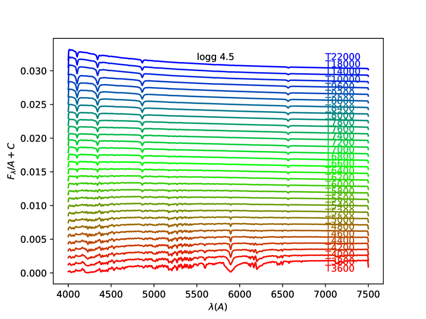
Figure 1: Sequence of 31 synthetic spectra computed with CSS and the VALD line list for $\log g=4.5$, $[{{\rm A}\over{\rm H}}]=0.0$ and $T_{\rm eff}$ values in the range 3600 to 22  000 K with $\Delta T_{\rm eff}$ intervals of 200 K for $T_{\rm eff}\leq 8000$ K and 400 K for $T_{\rm eff}>8000$ K.

3 Performance

The Slurm workload manager provided on the Digital Research Alliance of Canada (DRAC) parallel computing clusters allows for ”Array” jobs in which parts of the execution that can be automatically associated with a CPU identifier are automatically scattered to the corresponding CPUs. The spectrum synthesis calculations at a given $\lambda$ value are independent of those at another, and we use the Array job capability to automatically parallelize the wavelength domain of the spectrum synthesis. Because the density of spectral lines per unit $\Delta\lambda$ interval increases with decreasing $\lambda$ value, we distributed the splice points in the wavelength parallelization in approximately equal $\Delta\log\lambda$ intervals, finessed ad hoc to avoid splice points falling in the wings of lines that are broad in stars of the input stellar parameter values. For our performance test, we divided the $\lambda 400$ to $750$ nm range into eight logarithmic sub-ranges, each of which was handled by one of eight CPUs. Because spectrum synthesis is by far the slowest major stage in our integrated modeling process, we achieved a significant reduction in wall-clock time. The slurm ”sacct” and ”seff” reporting tools indicate CPU times and memory allocations ranging from 22 minutes and 0.7 Gbytes to 80 minutes and 1.2 Gbytes with both values generally increasing with decreasing $\lambda$ values of the assigned $\lambda$ range.

4 Comparison to standard stars

4.1 The Sun

Fig. 2 shows the continuum-normalized synthetic surface flux spectrum, $F_{\lambda}(\lambda)/F^{\rm C}_{\lambda}(\lambda)$, for a model of canonical grid input parameters close to those of the Sun of $(T_{\rm eff}/\log g/[{{\rm A}\over{\rm H}}])=(5800K/4.5/0.0)$ as computed with CSS and the NIST and with the VALD line lists. We have used the abundance distribution of Grevesse & Sauval (1998), adopted a microturbulent velocity dispersion, $\xi_{\rm T}$, of 1 km s^-1, and a Van der Waals broadening enhancement parameter, $\gamma_{\rm VW}$, of $\sim 3$. Also shown is the observed solar flux spectrum of (Kurucz, 2005) of spectral resolution, $R$, of $300\,000$ in a representative region around the Na I $D_{\rm 2}$ lines where the spectrum is relatively uncrowded. For this comparison we have smoothed the computed $F_{\lambda}(\lambda)$ distribution with with a Gaussian kernel with a $\sigma$ value of 2.0 km s^-1. Fig. 3 shows the same comparison for the more crowded Ca I 4227 line region. Fig. 4 shows the spectral energy distribution (SED) of the same model, projected from the Sun’s effective surface to the Earth’s distance to the Sun along with the observed solar irradiance spectrum of (Kurucz, 2006). For this comparison, both the observed and computed $F_{\lambda}$ distributions were broadened with a Gaussian kernel with a $\sigma$ value of 250 km s^-1 to allow an assessment of the realism with which the spectral structure is being modelled on the broadband scale. Fig. 5 shows the same comparison for the $\lambda 400$ to $500$ nm region where the Sun’s $F_{\lambda}$ distribution peaks. As seen in Figs. 4 and 5, the new larger line list provides for a more realistically line blanketed SED for GK stars in the $\lambda<500$ nm range where the SED becomes heavily blanketed and eventually over-blanketed with decreasing $\lambda$ value. Fig. 4 also shows the location of the ”Array job” splice points for the case of the Sun’s spectrum (see section 3).

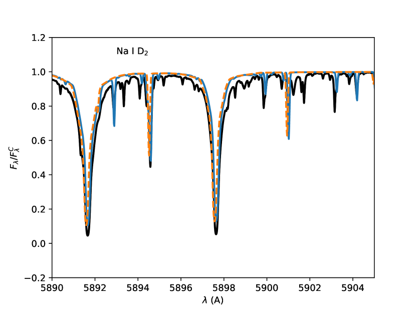
Figure 2: The observed and computed high resolution flux spectrum for the Sun in the Na I $D_{\rm 2}$ region. Observed spectrum of Kurucz et al. (1984) (black line); Synthetic spectra computed with ChromaStarServer (CSS) with the new VALD line list (solid blue line) and with the previous NIST line list (dashed orange line). The synthetic $F_{\lambda}$ spectra were broadened with a Gaussian kernel of $\sigma$ value of 2 km s^-1.

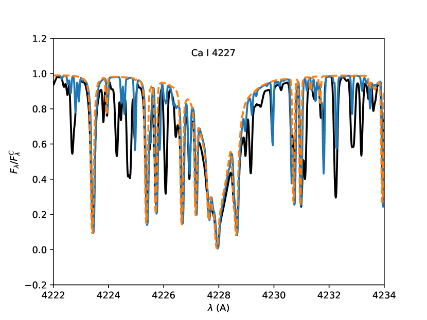
Figure 3: Same as Fig. 2 except for the Ca I 4227 line region.

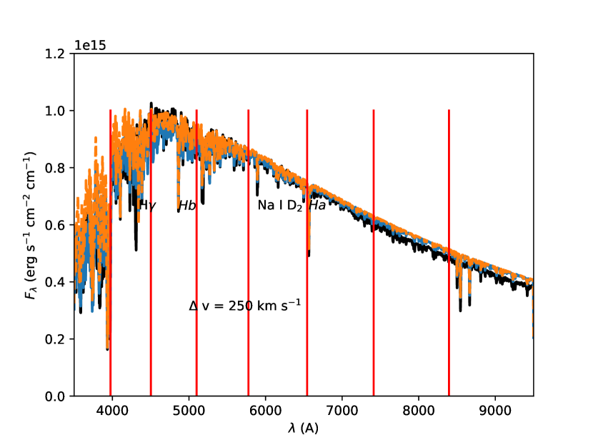
Figure 4: The observed and computed spectral energy distribution (SED) for the Sun. Observed spectral energy distribution (SED) of Kurucz (2006) (black line); Synthetic SEDs computed with ChromaStarServer (CSS) with the new VALD line list (solid blue line) and with the previous NIST line list (dashed orange line). The synthetic $F_{\lambda}$ spectra were broadened with a Gaussian kernel of $\sigma$ value of 250 km s^-1. The vertical lines indicate the splice points in the spectrum synthesis at which spectral sub-ranges were automatically scattered to different concurrently running CPUs.

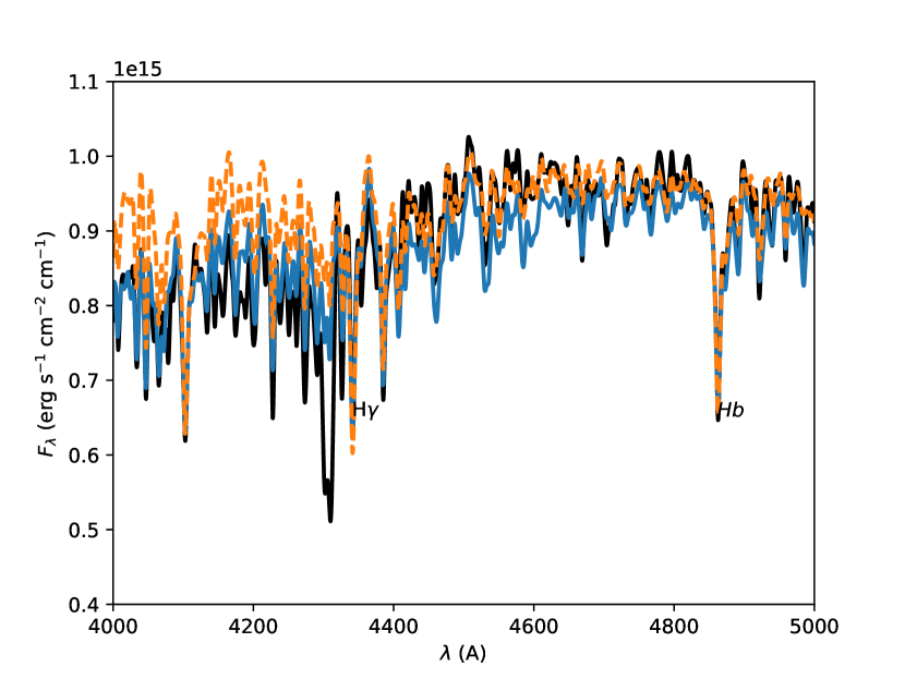
Figure 5: Same as Fig. 4 except for the $4000-5000$ Å  region where the solar SED reaches peak values.

$B-V$ color index

The additional line opacity has a small effect on the computed $B-V$ color, decreasing its value by $\sim 0.015$ mag. Fig. 6 shows the relative difference spectrum $(F^{\rm VALD}_{\lambda}-F^{\rm NIST}_{\lambda})/F^{\rm NIST}_{\lambda}$ along with the $BVR$ transmission curves and reveals that the additional VALD line opacity has a complicated distribution throughout the $B$ and $V$ bands. The synthetic $F_{\lambda}$ spectra were each broadened by convolution with a Gaussian kernel function with a $\sigma$ value of 100 km s^-1 before subtraction. The calibrated synthetic $B-V$, $V-R$, $V-I$, and $R-I$ color indices in the Johnson-Bessell system computed with the smaller NIST line list are $(0.365,0.717,1.355,0.277)$ whereas those computed with the new VALD line list are $(0.351,0.854,1.530,0.293)$. In both cases, the indices are calibrated with a single-point correction with a model of Vega computed with the VALD line list and input parameters of $(T_{\rm eff}/\log g/[{{\rm A}\over{\rm H}}])=(9550K/3.95/-0.5)$ (Castelli & Kurucz, 1994). For comparison, the color indices computed with our procedure from the observed solar irradiance spectrum of Kurucz (2006) are $(0.477,0.846,1.408,0.244)$.

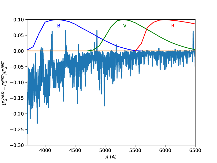
Figure 6: The relative difference of synthetic spectra computed with the VALD and NIST line lists, $(F^{\rm VALD}_{\lambda}-F^{\rm NIST}_{\lambda})/F^{\rm NIST}_{\lambda}$, in the $B-$ and $V-$ spectral regions computed for the Sun with the VALD and NIST line lists, overplotted with the scaled $B$, $V$, and $R$ transmission curves. The synthetic $F_{\lambda}$ spectra were broadened with a Gaussian kernel of $\sigma$ value of 100 km s^-1 before subtraction.

4.2 Arcturus

Figs. 7 and 8 show the $F_{\lambda}(\lambda)/F^{\rm C}_{\lambda}(\lambda)$ distribution for a model of canonical grid point input parameters and scaled solar abundances of $(T_{\rm eff}/\log g/[{{\rm A}\over{\rm H}}])=(4200K/1.5/-0.5)$ as computed with the VALD line list and smoothed with a Gaussian kernel with a $\sigma$ value of 4.0 km s^-1 along with the observed flux spectrum of Hinkle et al. (2000) of $R$ value $150\,000$ in the same Na I $D_{\rm 2}$ and Ca I 4227 regions. Peterson, Dalle Ore & Kurucz (1993) carried out a careful spectral analysis of Arcturus with an atomic line list calibrated with a solar model of the Sun’s spectrum, and found parameter values of $(T_{\rm eff}/\log g/[{{\rm Fe}\over{\rm H}}])=(4300K/1.5/-0.5)$ with enhanced abundances of the $\alpha$ elements of $+0.3$ dex. We note that to avoid damped spectral lines with wings that are grossly over-broadened, we reduced the $\gamma_{\rm VW}$ value to one (ie. no enhancement).

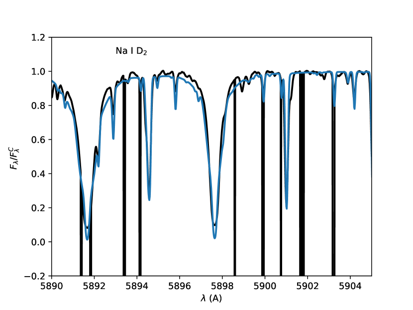
Figure 7: Same as Fig. 2 except for Arcturus. The observed spectrum (black) is that of Hinkle et al. (2000). The narrow bands where the observed flux is zero are artifacts in the published observed spectrum.

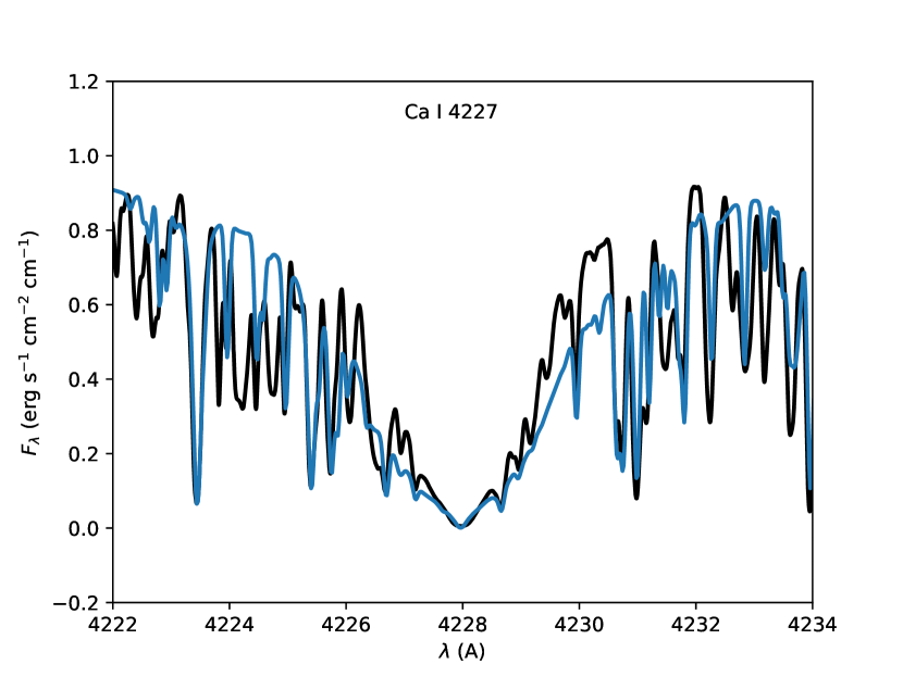
Figure 8: Same as Fig. 3 except for Arcturus. The observed spectrum (black) is that of Hinkle et al. (2000).

4.3 Vega

Fig. 9 shows the comparison between the observed high resolution spectrum of Vega of Takeda, Y. et al. (2007) and the synthetic spectrum computed with the VALD line list and the input parameters of Castelli & Kurucz (1994) and the updated H I broadening throughout the visible band. As reported in Section 2 we have re-tuned the H I Balmer line linear Stark broadening strengths to match the spectrum of Vega.

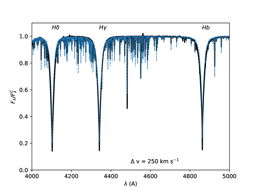
Figure 9: The observed and computed high resolution flux spectrum for Vega. Black line: observed spectrum of Takeda, Y. et al. (2007); solid blue line: CSS with the VALD line list. The synthetic $F_{\lambda}$ spectrum was broadened with a Gaussian kernel of $\sigma$ value of 20 km s^-1.

5 Comparison to Burke-Gaffney Observatory (BGO) spectra

The Burke-Gaffney Observatory (BGO, lat. $+44\,37\,50$, long. $-63\,34\,52$) at Saint Mary’s University (SMU) consists of a 0.6 m (24”) $f/6.5$ Planewave CDK24 telescope and is equipped with an $f/4$ model PF0035 ALPY 600 grism spectrograph from Shelyak Instruments. We operate the spectrograph with a slit width of 23 $\mu$m corresponding to a spectral resolving power, $R$, of $\sim 600$, equivalent to a spectral resolution element of $\Delta v\sim 500$ km s^-1 at $\lambda\sim 6000$ Å. The camera is a model Atik 314L+ CCD camera with $1391\times 1039$ imaging pixels of size $6.45\times 6.45$ $\mu$m. The setup provides a reciprocal linear dispersion, ${\Delta\lambda/\Delta x}$, of $\sim 420$ Å  mm^-1 and a spectral range, $\Delta\lambda$, of $\sim 3750$ Å, effectively covering the entire visible band from $\sim 4000$ to $\sim 7000$ Å  after accounting for edge effects.

5.1 Observations

Table 1 and Fig. 10 present a set of commissioning spectra of seven bright stars acquired on 15 April 2021 by the BGO Director and Astronomy Technician at the time, Mr. David Lane. The set includes six luminosity class V stars spanning the range of spectral class from K5 to B4 and one luminosity class III star of spectral class M3.

Table 1: Commissioning stars observed on 15 April 2021 with the ALPY 600 spectrograph. All stellar data are those of Hoffleit & Warren (1991)

Designation	$V$	$B-V$	Sp. Type	Exp. time (s)
HR3521	6.23	+1.62	M3 III	60
HR3580	6.44	-	K5 III	120
HR3309	6.32	+0.62	G5 V	120
HR4455	5.77	+0.46	F5 V	120
HR3333	5.95	+0.19	A5 V	60
HR3348	6.18	-0.03	A0 V	60
HR4456	5.95	-0.16	B4 V	120

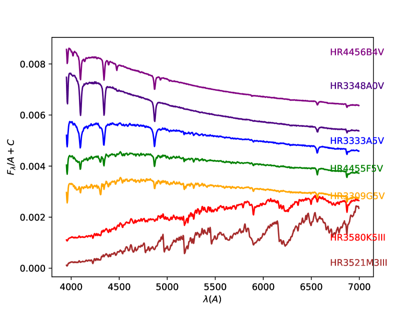
Figure 10: Set of seven commissioning spectra for the seven stars listed in Tab. 1 for the ALPY 600 spectrograph at the BGO.

5.2 Reduction procedure

This is the first presentation of BGO spectra in the research literature and in a companion paper Short, Lane & Fields (2023) we describe in detail our own locally developed BGO post-processing pipeline in the Python programming language for SMU students and present a brief summary here. The pipeline consists of automatic bias, dark current and flat-field corrections performed by software shipped with the ALPY 600 spectrograph. That is followed up by 1) Wavelength calibration by fitting a $2^{\rm nd}$-order polynomial to the relation ship between pixel columns and the known $\lambda$ value of Ar-Ne lines, 2) Subtraction of a $0^{\rm th}$-order fit to the remaining residual background to reduce the pedestal signal to zero, 3) Automatic location of the brightness peak in the cross-dispersion profile in sample columns across the chip, 4) Generation of a root-$N$ model cross-dispersion weight profile that is centered on the cross-dispersion peak in each column, 5) Formation of a $1D$ spectrum by summing columns weighted by the model profile from Step 4), 6) A two-step automatic approximate continuum rectification of the $\sim 4200$ to $6800$ Å  region that is designed for spectra unaffected by emission features or deep TiO bands (spectral classes B to K).

5.3 Comparison of BGO and CSS spectra

In Figs. 11, 12, and 13 we show the comparison between observed spectra from our BGO observing run and synthetic spectra from our model grid bracketing the nominal $T_{\rm eff}$ value corresponding to the spectral type listed in Hoffleit & Warren (1991). Nominal $T_{\rm eff}$ values were taken from Appendix G of Carroll & Ostlie (2007). Because we can only achieve an approximate continuum rectification for late type stars with high $\Delta\lambda/\Delta x$ broadband data, we do not attempt a quantitative fit based on minimizing a fitting statistic, but only a perform a visual inspection of the fit quality.

At the low $R$ and high ${{\Delta\lambda}\over{\Delta x}}$ values of these spectra, the main features at which we can assess the fit within the $\sim 4200$ to $\sim 6800$ Å  rectification range for GK stars are the Na I $D_{\rm 2}$ doublet at $\lambda 5900$ Å  and the TiO C${}_{\rm 3}\Delta$-X${}_{\rm 3}\Delta$ ($\alpha$ system, $\lambda_{\rm 00}~{}5170$ Å) and the B${}_{\rm 3}\Pi$-X${}_{\rm 3}\Delta$ ($\gamma$’ system, $\lambda_{\rm 00}~{}6193$ Å) bands. For A and B stars, at our $R$ and ${{\Delta\lambda}\over{\Delta x}}$ values, the main features at which we can judge the fit within the rectification range are the H I $\beta$ and $\gamma$ lines. This is sufficient to allow students to do projects at the undergraduate honours level in which they carry out and reduce their own BGO spectroscopy to coarsely classify stars to within a few spectral subclasses accuracy. In the process, they will gain valuable experience with the procedures of observational and computational stellar spectroscopy within a Python IDE running on commonplace Windows or Linux computer.

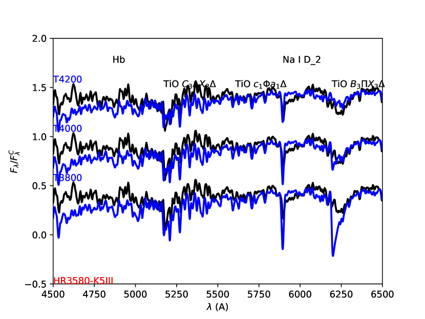
Figure 11: HR3580 (K5 III): Black: Observed spectrum from our BGO program plotted with three different vertical offsets. Blue: Synthetic spectra for models of $\log g=2.0$, $[{{\rm A}\over{\rm H}}]=0.0$, and $T_{\rm eff}$ values of 3800, 4000, and 4200 K in order of increasing vertical offset.

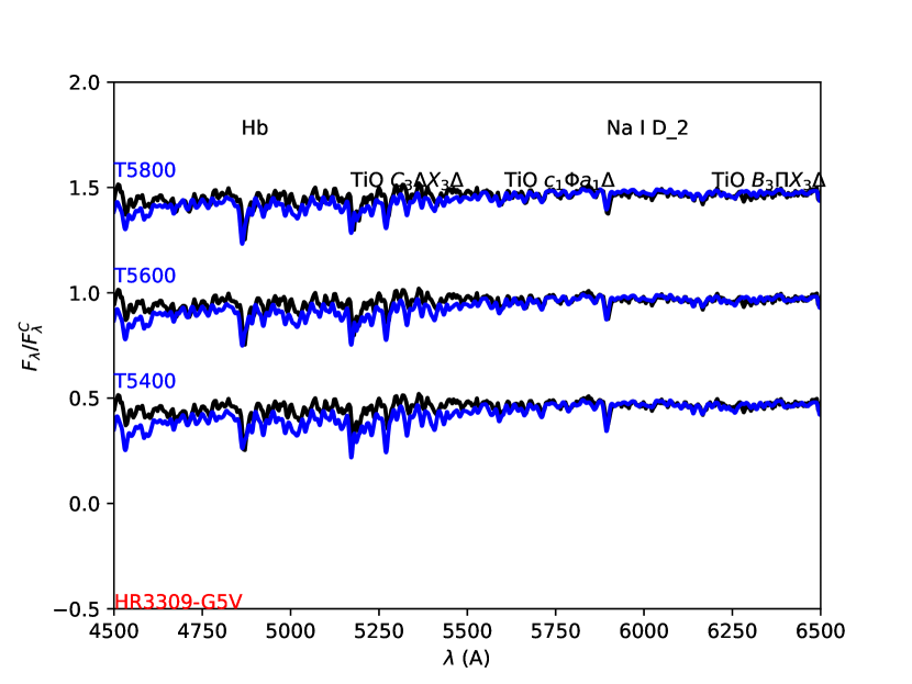
Figure 12: Same as Fig. 11 except for star HR3309 (G5 V) and models of $T_{\rm eff}$ values of 5400, 5600, and 5800 K.

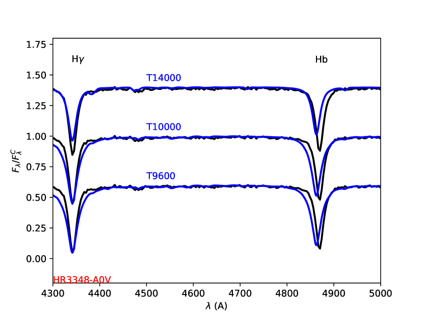
Figure 13: Same as Fig. 11 except for star HR3348 (A0 V) and models of $T_{\rm eff}$ values of 9600, 10000, and 14  000 K.

References

- Allard & Hauschildt (1995) Allard, F. & Hauschildt, P. H., 1995, The Astrophysical Journal, 445, 433
- Carroll & Ostlie (2007) Carroll, B.W. & Ostlie, D.A., 2007, An Introduction to Modern Astrophysics, 2nd Ed., Pearson - Addison Wesley (San Francisco)
- Castelli & Kurucz (1994) Castelli, F. & Kurucz, R.L., 1994,. Model atmospheres for VEGA, A&A, 281, 817
- Grevesse & Sauval (1998) Grevesse, N., Sauval, A.J., 1998, Space Science Reviews, 85, 161
- Harris et al. (2020) Harris, C.R., Millman, K.J., van der Walt, S.J. et al., 2020, Nature, 585, 357
- Hinkle et al. (2000) Hinkle, K., Wallace, L., Livingston, W., Ayres, T., Harmer, D., Valenti, J., 2003, The Future of Cool-Star Astrophysics: 12th Cambridge Workshop on Cool Stars, Stellar Systems, and the Sun, eds. A. Brown, G.M. Harper, and T.R. Ayres, University of Colorado, p. 851
- Hoffleit & Warren (1991) Hoffleit, D. & Warren, Jr W.H., 1991, The Bright Star Catalogue, 5th Rev. Ed.
- Kramida et al. (2015) Kramida, A., Ralchenko, Yu., Reader, J., and NIST ASD Team (2015). NIST Atomic Spectra Database (ver. 5.3), [Online]. Available: http://physics.nist.gov/asd [2015, November 26]. National Institute of Standards and Technology, Gaithersburg, MD.
- Kurucz (2006) Kurucz, R. L., 2006, arXiv:astro-ph/0605029
- Kurucz (2005) Kurucz, R. L., 2005, Memorie della Societa Astronomica Italiana Supplementi, 8, 189
- Kurucz et al. (1984) Kurucz, R. L., Furenlid, I., Brault, J., & Testerman, L. 1984, Solar Flux Atlas from 296 to 1300 nm (NSO Atlas 1; Sunspot: NSO)
- Pakhomov, Ryabchikova & Piskunov (2019) Pakhomov, Yu. V., Ryabchikova, T.A. & Piskunov, N.E., 2019, Astronomy Reports, 63, 1010
- Peterson, Dalle Ore & Kurucz (1993) Peterson, R.C., Dalle Ore, C.M., Kurucz, R.L., 1993, ApJ, 404, 333
- Piskunov & Valenti (2017) Piskunov, N. & Valenti, J.A., 2017, Astronomy & Astrophysics, 597, A16
- Ryabchikova et al. (2015) Ryabchikova, T., Piskunov, N., Kurucz, R. L., Stempels, H. C., Heiter, U., Pakhomov, Yu, Barklem, P. S., 2015, Physica Scripta, 90, 054005
- Short, Lane & Fields (2023) Short, C.I., Lane, D.J. & Fields, T., 2023, in press
- Short (2016) Short, C.I., 2016, PASP, 128, 104503
- Short & Bennett (2021) Short, C.I. & Bennett, P.D., 2021, PASP, 133, 064501
- Takeda, Y. et al. (2007) Takeda, Y., Kawanomoto, S. & and Ohishi, N., 2007, Publ. Astron. Soc. Japan, 59, 245
- Zeidler-K.T. & Koester (1982) Zeidler-K.T, E.M. & Koester, D., 1982, Astronomy & Astrophysics, 113, 173