Yang-Baxter Deformed Wedge Holography

Abstract

In this paper, we construct the wedge holography in the presence of homogeneous Yang-Baxter deformation. By doing so, we propose the co-dimension two holography in the context of deformed SYK model. We observe that the DGP term play a crucial role in obtaining the non-zero tension of the Karch-Randall branes in Yang-Baxter deformed wedge holography. The homogeneous Yang-Baxter deformation introduce non-trivial island surfaces inside the black hole horizon whose entanglement entropy is lower than the twice of thermal entropy of the black hole. Therefore, we obtain the Page curve even without the DGP term on the Karch-Randall branes due to the homogeneous Yang-Baxter deformation in the context of wedge holography. Finally, we compute the the holographic complexity in homogeneous Yang-Baxter deformed $AdS_{2}$ background.

1 Introduction

Duality is a robust proposal in physics. In string theory, the famous duality is the gauge-gravity duality. Gauge-gravity duality is helpful for exploring the strongly coupled gauge theories from the weakly coupled gravitational theories. J. Maldacena proposed the duality between type IIB string theory defined on $AdS_{5}\times S^{5}$ and ${\cal N}=4$ super Yang-Mills theory [1]. The gauge-gravity duality has been used in many branches of physics, e.g., condensed matter physics, cosmology, quantum chromodynamics (QCD), black hole information paradox, etc. The current paper is focused on the application of an extended version of this duality (wedge holography) to the black hole information paradox.

A very long time ago, Hawking found that black holes do not follow the unitary evolution of quantum mechanics [2, 3] which give rise to the information paradox. To recover the unitary evolution of black holes, entanglement entropy of Hawking radiation must follow the Page curve [4]. There has been extensive study on the information paradox using holography, and many proposals have been made (e.g. island proposal, double holography and wedge holography). The island proposal is based on the inclusion of contribution to the entanglement entropy from the interior of black holes at late times [5]. In early times, islands do not contribute to the entanglement entropy of the Hawking radiation, and one obtains the divergent entanglement entropy. These two phases together (no-island and island) reproduce the Page curve . The doubly holographic setup is constructed from the two copies of the usual AdS/CFT duality. In doubly holographic setups, the black hole is living on the end-of-the-world brane, and the external CFT bath acts as the sink to collect the Hawking radiation, see [16, 17, 18] and references therein. Another proposal is based on the wedge holography where the bath is taken as gravitating [21, 19, 20]. In doubly holographic setups and wedge holography, one obtains the Page curve from the entanglement entropies of the extremal surfaces: Hartman-Maldacena [22] and island surfaces. The wedge holography states the duality between classical gravity in the $(d+1)$-dimensional bulk and the $(d-1)$-dimensional CFT at the defect, i.e., wedge holography can be called co-dimension two holography.

In doubly holographic setup and wedge holography, some authors found that gravity is massive on the end-of-the-world brane [23, 24, 25, 26], and some authors showed that one could get the Page curve for the massless gravity in these models [27, 16, 28]. The authors in [27, 29, 30, 31] showed that the Page curve can be obtained in wedge holography by including the Dvali-Gabadadze-Porrati (DGP) term [32] on the Karch-Randall branes. However theories that includes DGP term on Karch-Randall branes belongs to the swampland [33] and these are not physical [34, 35]. The results of [16] have been obtained from a top-down approach for a non-conformal bath (thermal QCD bath) whose gravity dual is ${\cal M}$-theory inclusive of ${\cal O}(R^{4})$ corrections [36] and do not include the DGP term on the end-of-the-world brane. Recently one of the co-authors (GY) has figured out how to describe the Multiverse from the wedge holography [37] and discussed the application of [37] to the information paradox of black holes with multiple horizons and the grandfather paradox.

The purpose of the present paper is to explore the effects of the homogeneous Yang-Baxter deformation in the context of information paradox and holographic complexity. The importance of the YB deformations stems from the fact that they preserve the integrability of the sigma model [38, 39, 40, 41, 42]. Recently, the authors in [47, 48, 49] explore the effects of the novel YB deformations in the 2D-dilaton gravity system having a quadratic potential known as Almheiri-Polchinski (AP) model [50]. Interestingly, the authors found that the YB deformed $AdS_{2}$ background [47] could be a consistent solution of AP model if one deformed the quadratic potential into the hyperbolic function. The YB deformed $AdS_{2}$ metric plays a crucial role in the construction of YB deformed wedge holography. More concretely, in this paper

• We propose the co-dimension two holography for the deformed SYK model where the gravity dual is homogeneous Yang-Baxter deformed $AdS_{3}$.

• We explore the effect of the homogeneous Yang-Baxter deformation on the Page curve when the gravity dual is three-dimensional.

• Further, we investigate the effect of the homogeneous Yang-Baxter deformation on holographic complexity.

The paper is organized as follows. In section 2, we review the Almheiri-Polchinski (AP) Model and its Yang-Baxter deformation. In section 3, we construct wedge holography in the presence of homogeneous Yang-Baxter deformation via subsections 3.1 and 3.2: in subsection 3.1, we discuss the vacuum and black hole solutions in the presence of homogeneous Yang-Baxter deformation where as in subsection 3.2, we disucss the details of homogeneous Yang-Baxter deformed wedge holography. Section 4 compromises of two subsections: 4.1 and 4.2. In 4.1, we have shown that it is possible to get the Page curve in the presence of homogeneous Yang-Baxter deformation even without DGP term. In subsection 4.2, we have discussed the DGP term and swampland criteria in homogeneous Yang-Baxter deformed wedge holography. In section 5, we make comments that how one can obtain inhomogeneous Yang-Baxter deformed wedge holography. We compute the holographic complexity in homogeneous Yang-Baxter deformation in section 6 and then summarise our results in section 7. There are two appendices A and B on the computation of Hawking temperature and dimensional reduction from 3D to 2D respectively.

2 Review: Yang-Baxter Deformed Almheiri-Polchinski (AP) Model

In this section, we review the Yang-Baxter deformation of Almheiri-Polchinski Model and the discussion is based on [47]. We do the same in step by step as follows:

• $AdS_{2}$ as coset metric: $AdS_{2}$ has the following coset structure:

  $$AdS_{2}=SL(2)/U(1),$$ (1)

  coset representative $g$ has the following parametrization in terms of the coordinates $t$, $z$, time translation generator $H$ and dilatation generator $D$:

  $$g=e^{tH}e^{(logz)D}.$$ (2)

  One can write the $\mathfrak{sl}(2)$ algebra in conformal basis including the special conformal generator $C$ as follows:

  $$[D,H]=H,\ \ [C,H]=2D,\ \ [D,C]=-C.$$ (3)

  We can represent the generators of $\mathfrak{sl}(2)$ in terms of generators $T_{I}$ of $\mathfrak{so}(1,2)$ group with $I=0,1,2$ as:

  $$H\equiv T_{0}+T_{2},\ \ C\equiv T_{0}-T_{2},\ \ D\equiv T_{1},$$ (4)

  where following commutation relations hold for $T_{I}$’s:

  $$[T_{0},T_{1}]=-T_{2},\ \ [T_{1},T_{2}]=T_{0},\ \ [T_{2},T_{0}]=-T_{1}.$$ (5)

  $T_{I}$’s in the fundamental representation are given in terms of Pauli matrices ($\sigma_{i}(i=1,2,3)$) as:

  $$T_{0}=\frac{\iota}{2}\sigma_{1},\ \ \ ,T_{1}=\frac{\sigma_{2}}{2},\ \ \ T_{2}=\frac{\sigma_{3}}{2}.$$ (6)

  We can obtain the coset metric using left invariant one form $J$($=g^{-1}dg$) and projection operator $P(J)$ as:

  $$ds^{2}=2{\rm Tr}[JP(J)],$$ (7)

  where $J$ and $P(J)$ are defined as:

  $$J=e^{0}T_{0}+e^{1}T_{1}+\frac{1}{2}\omega^{01}T_{2},$$

  $$P(J)\equiv\frac{{\rm Tr}(JT_{0})}{{\rm Tr}(T_{0}T_{0})}T_{0}+\frac{{\rm Tr}(JT_{1})}{{\rm Tr}(T_{1}T_{1})}T_{1}$$ (8)

  where $J\in\mathfrak{sl}(2)$, $e^{0}$ and $e^{1}$ are zweibeins and $\omega^{01}$ is the spin connection. For the parametrization (2), zweibeins are given as:

  $$e^{0}=\frac{dt}{z},\ \ \ e^{1}=\frac{dz}{z}.$$ (9)

  Now using (• ‣ 2) and (9), coset metric (10) is simplified as:

  $$ds^{2}=2{\rm Tr}[JP(J)]=-e^{0}e^{0}+e^{1}e^{1}=\frac{-dt^{2}+dz^{2}}{z^{2}},$$ (10)

  which is $AdS_{2}$ metric.

• Prescription of Yang-Baxter Deformation: To deforme $AdS$ background we need to incorporate a factor in (7) as given below:

  $$ds^{2}=2{\rm Tr}\Biggl{[}J\frac{1}{1-2\eta R_{g}\circ P}P(J)\Biggr{]},$$ (11)

  where the constant parameter $\eta$ measures deformation and $R_{g}$ is defined as:

  $$R_{g}(X)\equiv g^{-1}\circ R(gXg^{-1})\circ g.$$ (12)

  A linear operator $R:\mathfrak{sl}(2)\rightarrow\mathfrak{sl}(2)$ satisfies the (modified) classical Yang-Baxter equation [(m)CYBE]:

  $$[R(X),R(Y)]-R\left([R(X),Y]+[X,R(Y)]\right)=c.[X,Y],$$ (13)

  where $c$ being the real constant parameter. When $c=0$ then one obtains homogeneous CYBE. For most general deformations, $R$ is defined as:

  $$R(T_{I})=\tilde{\Omega}_{IJ}M^{IJ}T_{K},$$ (14)

  where

  $$\tilde{\Omega}_{IJ}={\rm Tr}(T_{I}T_{J})=\frac{1}{2}\eta_{IJ},\ \ \ M^{IJ}=\begin{pmatrix}0&m_{1}&m_{2}\\ -m_{1}&0&m_{3}\\ -m_{2}&-m_{3}&0\end{pmatrix}.$$ (15)

  For the ansatz (14), equation (13) reduces to:

  $$-m_{1}^{2}-m_{2}^{2}+m_{3}^{2}=4c.$$ (16)

  Using (11) and (14), Yang-Baxter deformed $AdS_{2}$ metric is obtained as:

  $$ds^{2}=\frac{-dt^{2}+dz^{2}}{z^{2}-\eta^{2}\left(\alpha+\beta t+\gamma(-t^{2}+z^{2})\right)^{2}},$$ (17)

  where

  $$\alpha=\frac{m_{1}+m_{3}}{2},\ \ \beta=-m_{2},\ \ \gamma=\frac{m_{1}-m_{3}}{2}.$$ (18)

  Metric (17) produces the following Ricci scalar,

  $$R=-2\left(1-\tilde{\omega}\eta^{2}\right)\frac{z^{2}+\eta^{2}\left(\alpha+\beta t+\gamma(-t^{2}+z^{2})\right)^{2}}{z^{2}-\eta^{2}\left(\alpha+\beta t+\gamma(-t^{2}+z^{2})\right)^{2}},$$ (19)

  with $\tilde{\omega}=\beta^{2}+4\alpha\gamma=m_{1}^{2}+m_{2}^{2}-m_{3}^{2}=-4c$. In $\eta\rightarrow 0$ limit, $R=-2$, however deformed geometry contains both AdS and dS depending upon the values of parameters and coordinates. For homogeneous Yang-Baxter deformation, $\beta=\gamma=0$ implying $\tilde{\omega}=0$.

• Almheiri-Polchinski (AP) Model: AP model is described by the following action:

  $$S=\frac{1}{16\pi G_{N}^{(2)}}\int d^{2}x\sqrt{-g}\left(\Phi^{2}R-\left(2-2\Phi^{2}\right)\right)+\frac{1}{32\pi G_{N}^{(2)}}\int d^{2}x\sqrt{-g}(\nabla f)^{2},$$ (20)

  where $G_{N}^{(2)}$ being the two dimensional Newton constant and second term is the matter part of the action. Vacuum solution of AP model is given as [50]:

  $$ds^{2}=\frac{1}{z^{2}}\left(-dt^{2}+dz^{2}\right),$$

  $$\Phi^{2}=1+\frac{a+bt+c(-t^{2}+z^{2})}{z},$$ (21)

  where $a,b,c$ are real constants. Parameters, $a=1/2,\ b=0,\ c=\mu/2$(with $\mu$ as a real positive constant) correspond to a black hole solution:

  $$ds^{2}=-4\left(\rho^{2}-\mu\right)dt^{2}+\frac{d\rho^{2}}{\rho^{2}-\mu},$$

  $$\Phi^{2}=1+\rho,$$ (22)

  where horizon of black hole (• ‣ 2) is at $\rho=\sqrt{\mu}$. Hawking temperature and Bekenstein-Hawking entropy are given as:

  $$T_{H}^{\rm AP}=\frac{\sqrt{\mu}}{\pi},\ \ \ \ \ S_{\rm BH}^{\rm AP}=\frac{\Phi^{2}}{4G}\Biggl{|}_{\rho=\sqrt{\mu}}=\frac{1+\sqrt{\mu}}{4G_{N}^{(2)}}.$$ (23)

• Yang-Baxter Deformed AP Model: Using the presciption of Yang-Baxter deformation as described earlier, authors obtained the deformation of AP model as given below [47]:

  • Vacuum Solution: Metric, dilaton and potential are given as [47]:

    $$ds^{2}=\frac{1}{1-\eta^{2}(X.P)^{2}}\frac{-dt^{2}+dz^{2}}{z^{2}},\ \ \Phi^{2}=\frac{1}{2\eta}\log\Biggl{|}\frac{1+\eta(X.P)}{1-\eta(X.P)}\Biggr{|}+1,$$

    $$U(\Phi)=-(1-\tilde{\omega}\eta^{2})\frac{1}{\eta}\sinh[2\eta(\Phi^{2}-1)],\ \ \ [{\rm when}\ 1>|\eta(X.P)|],$$

    $$U(\Phi)=(1-\tilde{\omega}\eta^{2})\frac{1}{\eta}\sinh[2\eta(\Phi^{2}-1)],\ \ \ \ \ \ [{\rm when}\ 1<|\eta(X.P)|],$$ (24)

    where

    $$X.P=\frac{\alpha+\beta t+\gamma(-t^{2}+z^{2})}{z}.$$ (25)

    $\beta=\gamma=0$ corresponds to homogeneous Yang-Baxter deformation. Use has been made of

    $$X^{I}=\frac{1}{z}\left(t,\frac{1}{2}(1+t^{2}-z^{2}),\frac{1}{2}(1-t^{2}+z^{2})\right),$$

    $$P_{I}=\left(\beta,\alpha-\gamma,\alpha+\gamma\right),$$

    $$X.P=X^{I}P_{I}=\frac{\alpha+\beta t+\gamma(-t^{2}+z^{2})}{z}.$$ (26)

    Further, $\eta_{IJ}={\rm diag}(-1,+1,-1)$, $X.X=\eta_{IJ}X^{I}X^{J}=-1$ and $P.P=\eta^{IJ}P_{I}P_{J}=-\tilde{\omega}$.

  • Black Hole Solution: For the black hole solution, $\mu=-\tilde{P}.\tilde{P}=\tilde{\omega}=4c$. Since, $\tilde{\omega}\neq 0$ and therefore this is an inhomogeneous black hole solution:

    $$ds^{2}=-4F(r)dt^{2}+\frac{dr^{2}}{F(r)},\ \ \ \ \ \Phi^{2}=1+r,$$ (27)

    where

    $$F(r)=\frac{-1-\eta^{2}\mu+(1-\eta^{2}\mu)\cosh(2\eta r)}{2\eta^{2}}.$$ (28)

    Boundary of (27) is located at $r=\infty$ and horizon is located at $r=r_{h}=\frac{1}{\eta}{\rm tanh^{-1}}(\eta\sqrt{\mu})$. Hawking temperature and Bekenstein-Hawking entropy for (27) are given by:

    $$T_{H}^{\rm AP,\eta}=\frac{\sqrt{\mu}}{\pi},\ \ \ \ \ \ S_{\rm BH}^{\rm AP,\eta}=\frac{1+r_{h}}{4G_{N}^{(2)}}=\frac{1}{4G_{N}^{(2)}}+\frac{{\rm tanh^{-1}}(\eta\sqrt{\mu})}{4G_{N}^{(2)}\eta}.$$ (29)

Before proceed further, we would like to make it clear that in this paper, we discuss only homogeneous Yang-Baxter deformation.

3 Wedge Holography in Homogeneous Yang-Baxter Deformed Model

Working action for the wedge holography with $AdS_{3}$ bulk is written as follows:

$$S=\frac{1}{16\pi G_{N}^{(3)}}\Biggl{[}\int_{M}d^{3}x\sqrt{-g^{(3)}}(R-2\Lambda)+2\int_{\partial M}d^{2}x\sqrt{-h}K+2\int_{Q_{\gamma}}d^{2}x\sqrt{-h_{\gamma}}\left({\cal K}_{\gamma}-T_{\gamma}\right)\Biggr{]},$$ (30)

where the first term of the above equation is Einstein Hilbert term with negative cosmological constant [51], second term is the Gibbons-Hawking-York boundary term, and third term is defined on the Karch-Randall branes with $\gamma=1,2$ located at constant $\theta$ (we will see soon) where Karch-Randall branes have induced metric $h_{\gamma}$ and tensions $T_{\gamma}$. On varying the action (30) with respect to space-time ($g_{\mu\nu}$), we obtain the Einstein equation:

$${\rm EOM}_{\mu\nu}:\ R_{\mu\nu}-\frac{R}{2}g_{\mu\nu}+\Lambda g_{\mu\nu}=0.$$ (31)

Next we compute the Neumann boundary condition (NBC) which can be obtained by varying (30) with respect to the metric $h_{ij}$

$${\cal K}_{ij}^{\gamma}-({\cal K}^{\gamma}-T^{\gamma})h_{ij}^{\gamma}=0,$$ (32)

where ${\cal K}_{ij}^{\gamma}=\frac{1}{2}n^{\theta}\partial_{\theta}{g_{ij}^{\gamma}}|_{\theta=\theta_{1},\pi-\theta_{2}}$; $\theta=\theta_{1},\pi-\theta_{2}$ denote the locations of the two Karch-Randall (KR) branes, see Fig. 1.

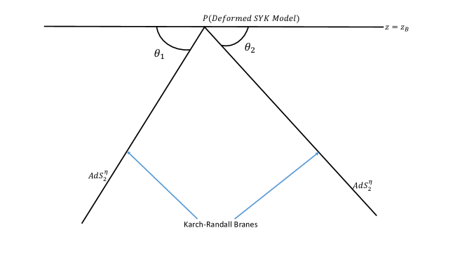
Figure 1: Pictorial realization of homogeneous Yang-Baxter deformed wedge holography. $z_{B}$ is the holographic screen and $P$ is the defect.

Before start discussing the construction of wedge holography, let us first discuss the vacuum and black hole solutions of Einstein’s equation (31).

3.1 Basics

• Vacuum solution: Vacuum solution of the bulk Einstein’s equation (31) of the action (30) is given by [51]:

  $$ds^{2}_{\eta}={\cal F}_{\eta}(z)\Biggl{(}\frac{-dt^{2}+dz^{2}}{z^{2}}\Biggr{)}+{\cal G}_{\theta\theta}^{\eta}d\theta^{2},$$ (34)

  where

  $${\cal F}_{\eta}(z)=\frac{1}{1-\frac{\eta^{2}\alpha^{2}}{z^{2}}};\ \ \ \ {\cal G}_{\theta\theta}^{\eta}=\Biggl{[}\frac{1}{2\eta}\log\Biggl{(}\frac{1+\frac{\eta\alpha}{z}}{1-\frac{\eta\alpha}{z}}\Biggr{)}+1\Biggr{]}^{2},$$ (35)

  where $\eta$ is the Yang-Baxter deformation parameter. Notice that the above solution satisfies the equations of motion provided the following constraint holds:

  $$2\eta+\log\Bigg{[}\frac{z+\alpha\eta}{z-\alpha\eta}\Bigg{]}-\frac{2z\alpha\eta}{z^{2}-\alpha^{2}\eta^{2}}=0$$ (36)

  and we stay infinitesimally away from the boundary i.e. $z_{B}=\eta\alpha+\epsilon$, where $\epsilon\gtrsim O(\alpha)$. Lets verify this explicitly. LHS of EOMs (31) for the solution (34) are obtained as:

  $${\rm EOM}_{tt}^{\rm LHS}=\frac{-\alpha^{2}\eta^{2}+z^{2}-\frac{2\alpha\eta z}{2\eta+\log\left(\frac{\alpha\eta+z}{z-\alpha\eta}\right)}}{(z-\alpha\eta)^{2}(\alpha\eta+z)^{2}},$$

  $${\rm EOM}_{zz}^{\rm LHS}=\frac{\alpha^{2}\eta^{2}-z^{2}+\frac{2\alpha\eta z}{2\eta+\log\left(\frac{\alpha\eta+z}{z-\alpha\eta}\right)}}{(z-\alpha\eta)^{2}(\alpha\eta+z)^{2}},$$

  $${\rm EOM}_{\theta\theta}^{\rm LHS}=\frac{\alpha^{2}\left(2\eta+\log\left(\frac{\alpha\eta+z}{z-\alpha\eta}\right)\right)^{2}}{2(z-\alpha\eta)(\alpha\eta+z)}.$$ (37)

  Upon imposing constraint (36), we see that:

  $${\rm EOM}_{tt}^{\rm LHS}=0,$$

  $${\rm EOM}_{zz}^{\rm LHS}=0,$$

  $${\rm EOM}_{\theta\theta}^{\rm LHS}=\frac{2\alpha^{4}\eta^{2}z^{2}}{\left(z^{2}-\alpha^{2}\eta^{2}\right)^{3}}.$$ (38)

  We can rewrite ${\rm EOM}_{\theta\theta}$ after performing small $\eta$ expansion as:

  $${\rm EOM}_{\theta\theta}^{\rm LHS}=\frac{2\alpha^{4}\eta^{2}}{z^{4}}+\frac{6\alpha^{6}\eta^{4}}{z^{6}}+O\left(\eta^{5}\right).$$ (39)

  Now if we stay slightly away from boundary holographic screen, i.e., $z_{B}=\eta\alpha+\epsilon$, then the leading order term in (39) takes the form: $\frac{2\alpha^{4}\eta^{2}}{(\eta\alpha+\epsilon)^{4}}\approx\frac{2\alpha^{4}\eta^{2}}{\epsilon^{4}}$ which is vanishingly small.

• Black hole solution: We compute the consistent Yang-Baxter deformed black hole solution associated with (30). On solving (31), we obtain

  $$ds^{2}_{\eta}={\cal F}_{\eta}(z)\Biggl{(}\frac{-f(z)dt^{2}+\frac{dz^{2}}{f(z)}}{z^{2}}\Biggr{)}+{\cal G}_{\theta\theta}^{\eta}d\theta^{2},$$ (40)

  where

  $$f(z)=1-\frac{z^{2}}{z_{h}^{2}}\hskip 2.84526pt.$$ (41)

  Here, $z_{h}$ denotes the location of the black hole horizon. We obtained the LHS of EOMs (31) for the black hole solution (40) as written below:

  $$\hskip-14.45377pt{\rm EOM}_{tt}^{\rm LHS}=\frac{f(z)\left((z-\alpha\eta)(\alpha\eta+z)\left(\alpha\eta f^{\prime}(z)+2\eta+\log\left(\frac{\alpha\eta+z}{z-\alpha\eta}\right)\right)-2\alpha\eta zf(z)\right)}{\left(z^{2}-\alpha^{2}\eta^{2}\right)^{2}\left(2\eta+\log\left(\frac{\alpha\eta+z}{z-\alpha\eta}\right)\right)},$$

  $$\hskip-14.45377pt{\rm EOM}_{zz}^{\rm LHS}=\frac{2\alpha\eta zf(z)-(z-\alpha\eta)(\alpha\eta+z)\left(\alpha\eta f^{\prime}(z)+2\eta+\log\left(\frac{\alpha\eta+z}{z-\alpha\eta}\right)\right)}{f(z)\left(z^{2}-\alpha^{2}\eta^{2}\right)^{2}\left(2\eta+\log\left(\frac{\alpha\eta+z}{z-\alpha\eta}\right)\right)},$$

  $$\hskip-14.45377pt{\rm EOM}_{\theta\theta}^{\rm LHS}=-\frac{\left(2\eta+\log\left(\frac{\alpha\eta+z}{z-\alpha\eta}\right)\right)^{2}}{8\eta^{2}(\alpha\eta-z)(\alpha\eta+z)}\Biggl{(}(z-\alpha\eta)(\alpha\eta+z)\left(f^{\prime\prime}(z)(z-\alpha\eta)(\alpha\eta+z)-2zf^{\prime}(z)-2\right)$$

  $$\hskip 180.67499pt+2f(z)\left(\alpha^{2}\eta^{2}+z^{2}\right)\Biggr{)}$$ (42)

  It should be noted that the above black hole solution (40) satisfies the equations of motion (31) up to the following constraint:

  $$2\eta+\log\Bigg{[}\frac{z+\alpha\eta}{z-\alpha\eta}\Bigg{]}-\frac{2z\alpha\eta f(z)}{z^{2}-\alpha^{2}\eta^{2}}+\alpha\eta f^{\prime}(z)=0,$$ (43)

  and the black hole horizon must be located far away from the $\alpha\eta$, i.e., $z_{h}>>\alpha\sqrt{\eta}$. We can see this explicitly as follows. For the constraint (43), (• ‣ 3.1) reduces to:

  $${\rm EOM}_{tt}^{\rm LHS}=0,$$

  $${\rm EOM}_{zz}^{\rm LHS}=0,$$

  $${\rm EOM}_{\theta\theta}^{\rm LHS}=\frac{\left(\alpha F^{\prime}(z)(z-\alpha\eta)(\alpha\eta+z)-2\alpha zF(z)\right)^{2}}{8\left(z^{2}-\alpha^{2}\eta^{2}\right)^{3}}\Biggl{(}(z-\alpha\eta)(\alpha\eta+z)$$

  $$\hskip 72.26999pt\left(F^{\prime\prime}(z)(z-\alpha\eta)(\alpha\eta+z)-2zF^{\prime}(z)-2\right)+2F(z)\left(\alpha^{2}\eta^{2}+z^{2}\right)\Biggr{)}.$$ (44)

  Small $\eta$ expansion of ${\rm EOM}_{\theta\theta}^{\rm LHS}$ appearing in (• ‣ 3.1) leads to the following equation:

  $${\rm EOM}_{\theta\theta}^{\rm LHS}=-\frac{(z^{2}-2z_{h}^{2})\alpha^{4}\eta^{2}}{z^{4}z_{h}^{4}}+O(\eta^{4}).$$ (45)

  Near horizon expansion of the leading order term appearing in (45) is given as:

  $${\rm EOM}_{\theta\theta}^{\rm LHS}=\frac{\alpha^{4}\eta^{2}}{z_{h}^{4}}-\frac{6\alpha^{4}\eta^{2}}{z_{h}^{5}}(z-z_{h})+O(z-z_{h})^{2}.$$ (46)

  Hence, ${\rm EOM}_{\theta\theta}^{\rm LHS}$ is vanishingly small when $z_{h}>>\alpha\sqrt{\eta}$.

• Thermal entropy: The black hole solution defined in (40) has the following thermal entropy:

  $$S_{\rm thermal}=\frac{A_{z=z_{h}}}{4G_{N}^{(3)}}=\frac{\int_{\theta_{1}}^{\pi-\theta_{2}}d\theta\sqrt{{\cal G}_{\theta\theta}^{\eta}}|_{z=z_{h}}}{4G_{N}^{(3)}}=\frac{\left(\pi-(\theta_{2}+\theta_{1})\right){\sqrt{{\cal G}_{\theta\theta}^{\eta}}|_{z=z_{h}}}}{4G_{N}^{(3)}}.$$ (47)

  Alternatively, one can compute the thermal entropy of $3D$ black holes using the Wald method [52, 53]. Wald entropy or the Noether charge entropy for stationary black holes is defined as:

  $$S_{W}=-2\pi\oint_{\Sigma}\Bigg{(}\frac{\delta\mathcal{L}}{\delta R_{abcd}}\Bigg{)}\epsilon_{ab}\epsilon_{cd}\overline{\epsilon},$$ (48)

  where $\epsilon_{ab}$ is the anti-symmetric tensor with the normalisation condition $\epsilon_{ab}\epsilon^{ab}=-2$ and the integral is evaluated on the $D-2$ dimensional bifurcation surface $\Sigma$. For our case, the bifurcation surface is at $z=z_{h}$ and $t=t_{0}$, where $z_{h}$ is the location of horizon and $t_{0}$ is a constant. Furthermore, the derivative in (48) is evaluated using the on-shell condition.

  Using (30) and (48), we obtain

  $$S_{W}=-\frac{1}{8\pi G_{N}^{(3)}}\oint_{\Sigma}g^{ac}g^{bd}\epsilon_{ab}\epsilon_{cd}\sqrt{\mathcal{G}_{\theta\theta}^{\eta}}d\theta=\frac{\left(\pi-(\theta_{2}+\theta_{1})\right)}{4G_{N}^{(3)}}\sqrt{\mathcal{G}_{\theta\theta}^{\eta}}\Big{|}_{z=z_{h}},$$ (49)

  which is identical to thermal entropy obtained in (47).

  Using (35), (43) and (47), the thermal entropy of the black hole phase can be estimated as

  $$S_{\rm thermal}=-\frac{\left(\pi-(\theta_{2}+\theta_{1})\right)\alpha f^{\prime}(z_{h})}{8G_{N}^{(3)}}=\frac{\left(\pi-(\theta_{2}+\theta_{1})\right)\alpha}{4G_{N}^{(3)}}.$$ (50)

3.2 Wedge Holography in the Presence of Homogeneous Yang-Baxter deformation

Wedge holography in three dimensional bulk exists provided following conditions should be satisfied [54, 55]:

• Bulk metric should satisfy Einstein’s equation with a negative cosmological constant in three dimensions (31).

• Bulk metric should satisfy Neumann boundary conditions (32) on the Karch-Randall branes.

• Metric ($h_{ij}$) on Karch-Randall branes should satisfy Einstein’s equation with a negative cosmological constant in two dimensions:

  $$R_{ij}-\frac{R[h_{ij}]}{2}h_{ij}+\Lambda h_{ij}=0.$$ (51)

Tensions of Karch-Randall Branes without DGP Term: In this case, bulk action is (30). For general metric, NBC (32) is satisfied provided, $T^{\gamma}={\cal K}^{\gamma}-\frac{{\cal K}_{ij}^{\gamma}}{h_{ij}^{\gamma}}$. For vacuum solution (34) and black hole solutin (40), $K_{ij}^{\gamma}=0$, and hence ${\cal K}^{\gamma}=0$, therefore (32) implying

$$T^{\gamma}h_{ij}^{\gamma}=0.$$ (52)

Notice that, $h_{ij}^{\gamma}\neq 0$, and hence $T_{\gamma}=0$, i.e., Karch-Randall branes are tensionless without DGP term.

Tensions of Karch-Randall Branes in the Presence of DGP Term: In the presence of the DGP term on the Karch-Randall branes, gravitational action (30) is modified as [27]:

$$\hskip-14.45377ptS=\frac{1}{16\pi G_{N}^{(3)}}\Biggl{[}\int_{M}d^{3}x\sqrt{-g^{(3)}}\left(R[g]-2\Lambda\right)+2\int_{\partial M}d^{2}x\sqrt{-h}K+2\int_{Q_{\gamma}}d^{2}x\sqrt{-h_{\gamma}}\left({\cal K}_{\gamma}-T_{\gamma}+\lambda_{\gamma}R_{h_{\gamma}}\right)\Biggr{]},$$ (53)

where all the terms in (53) are same as defined in (30) except $R_{h_{\gamma}}$, which are intrinsic curvature scalars on two Karch-Randall branes. In this case, bulk metric satisfies the following Neumann boundary condition at $\theta=\theta_{1},\pi-\theta_{2}$:

$${\cal K}_{\gamma,ij}-({\cal K}_{\gamma}-T_{\gamma}+\lambda_{\gamma}R_{h_{\gamma}})h_{\gamma,ij}+2\lambda_{\gamma}R_{\gamma,{ij}}=0.$$ (54)

The general bulk metric satisfies Neumann boundary condition (54) provided tensions of the Karch-Randall branes in the presence of DGP term should be given as follows:

$$T_{\gamma}={\cal K}_{\gamma}-\frac{{\cal K}_{\gamma,ij}}{h_{\gamma,ij}}+\lambda_{\gamma}R_{h_{\gamma}}-\frac{2\lambda_{\gamma}R_{\gamma,{ij}}}{h_{\gamma,ij}}.$$ (55)

For the bulk metric (34), equation (55) simplifies to the following form:

$$T_{\gamma}=\lambda_{\gamma}\left(R_{h_{\gamma}}-\frac{2R_{\gamma,{ij}}}{h_{\gamma,ij}}\right).$$ (56)

For the given metric (34), the Ricci tensor and Ricci scalar on the Karch-Randall branes are obtained as:

$$R_{11}=\frac{-\alpha^{4}\eta^{4}+4\alpha^{2}\eta^{2}z^{2}+z^{4}}{\left(z^{3}-\alpha^{2}\eta^{2}z\right)^{2}},$$

$$R_{22}=\frac{\alpha^{4}\eta^{4}-4\alpha^{2}\eta^{2}z^{2}-z^{4}}{\left(z^{3}-\alpha^{2}\eta^{2}z\right)^{2}},$$

$$R_{h_{1}}=R_{h_{2}}=-2-\frac{8\alpha^{2}\eta^{2}}{z^{2}}+\frac{2\alpha^{4}\eta^{4}}{z^{4}}.$$ (57)

Now we define $\kappa=\eta\alpha$, and using (3.2), tensions of the branes (56) turn out to be of the following form:

$$T_{1}=2{\lambda_{1}}+\frac{8\kappa^{2}{\lambda_{1}}}{z^{2}}-\frac{2\kappa^{4}{\lambda_{1}}}{z^{4}}+O\left(\kappa^{6}\right),$$

$$T_{2}=2{\lambda_{2}}+\frac{8\kappa^{2}{\lambda_{2}}}{z^{2}}-\frac{2\kappa^{4}{\lambda_{2}}}{z^{4}}+O\left(\kappa^{6}\right).$$ (58)

Notice that when $\lambda_{1}=\lambda_{2}$ then both Karch-Randall branes have same tensions. From (3.2), we conclude that, the presence of the DGP term generates the tensions on Karch-Randall branes in the Yang-Baxter deformed wedge holography.

Therefore, we see that bulk metric (34) and (40) satisfy Neumann boundary conditions on the Karch-Randall branes provided Karch-Randall branes should be tensionless and tensive in the absence and presence of DGP term respectively. Now, since all the conditions required for the existence of wedge holography are satisfied. Therefore, we now discuss the description of homogeneous Yang-Baxter deformed wedge holography.

Description of Homogeneous Yang-Baxter deformed Wedge Holography: Wedge holography has been discussed in the context of compact angle in [25]. Let us briefly review the same here. The bulk metric has the following form:

$$ds^{2}=\frac{1}{\sin^{2}\mu}\left(\frac{-dt^{2}+du^{2}+d\vec{x}^{2}}{u^{2}}+d\mu^{2}\right),$$ (59)

where $u>0$, $\vec{x}=(x^{1},x^{2},......,x^{d-2})$ [$d-2$ real transverse directions] and $\mu\in(0,\pi)$. In the bulk (59), Karch-Randall branes are located at $\mu=\theta_{1}$ and $\mu=\pi-\theta_{2}$ [see Fig. 1 of [25]]. The geometry on the Karch-Randall branes is $AdS_{d}$. The setup constructed by us has the similar scenario. In our case, the compact direction is $\theta$, and the Karch-Randall branes have $AdS_{2}^{\eta}$ geometry. The difference between [25] and our setup is the absence of $d-2$ transverse direction in this work. For the black hole case, there will be black hole function in the metric (59):

$$ds^{2}=\frac{1}{\sin^{2}\mu}\left(\frac{-h(u)dt^{2}+\frac{du^{2}}{h(u)}+d\vec{x}^{2}}{u^{2}}+d\mu^{2}\right),$$ (60)

where $h(u)=1-\frac{u^{d-1}}{u_{h}^{d-1}}$.

Wedge holography in the presence of homogeneous Yang-Baxter deformation can be constructed as follows. We have two Karch-Randall branes located at $\theta=\theta_{1}$, $\theta=\pi-\theta_{2}$ and these branes are joined at the one-dimensional defect $(P)$ as shown in Fig. 1. In this setup, the non-conformal boundary of the $3D$ bulk is located at the holographic screen placed at $z=z_{B}$. The homogeneous Yang-Baxter deformed wedge holography has the following three descriptions.

• Boundary description: Two-dimensional non-conformal field theory (NCFT) at the holographic screen ($z=z_{B}$) with one-dimensional boundary. We call the NCFT located at the holographic screen as “holographic screen non-conformal field theory (HSNCFT)”.

• Intermediate description: Gravitating systems with homogeneous Yang-Baxter deformed $AdS_{2}$ geometries (KR-branes) are connected to each other via transparent boundary conditions at the defect.

• Bulk description: HSNCFT located at the holographic screen ($z=z_{B}$) has three-dimensional gravity dual.

In our setup, the dictionary of wedge holography in the presence of homogeneous Yang-Baxter deformation can be schematically expressed as:

Classical gravity in three-dimensional homogeneous Yang-Baxter deformed $AdS_{3}$ bulk
$\equiv$ (Quantum) gravity on two Karch-Randall branes with metric homogeneous Yang-Baxter deformed $AdS_{2}$
$\equiv$ deformed SYK model living at the one-dimensional defect.

The relationship between the first and second lines is because of the braneworld holography [58, 59]. The third line is related to the second line due to JT/SYK duality [60, 61, 62, 63, 64, 65, 66, 67, 68, 69]. Therefore, classical gravity in homogeneous Yang-Baxter deformed $AdS_{3}$ can be dual to deformed SYK model at the one-dimensional defect based on wedge holography [21, 19, 20].

4 Information Paradox in Homogeneous Yang-Baxter Deformed Wedge Holography

In this section, we use the wedge holography constructed in section 3 to discuss the Page curve of black holes in the homogeneous Yang-Baxter deformed wedge holography in 4.1. and in 4.2 we discuss the DGP term and swampland criteria in homogeneous Yang-Baxter deformed wedge holography.

4.1 Page Curve Due to the Presence of Homogeneous Yang-Baxter Deformation

In this subsection, we explore the Page curve of the eternal black hole in the absence of the DGP term on the Karch-Randall branes. For this purpose, we consider the two extremal surfaces: Hartman-Maldacena, and island surfaces, and calculate their respective entanglement entropies in 4.1.1 and 4.1.2.

4.1.1 Hartman-Maldacena Surface’s Entanglement Entropy

Let us write the bulk metric (40) in terms of the infalling Eddington-Finkelstein coordinate, $dv=dt-\frac{dz}{f(z)}$ as below:

$$ds_{(2+1)}^{2}=g_{\mu\nu}dx^{\mu}dx^{\nu}={\cal G}_{\theta\theta}^{\eta}d\theta^{2}+{{\cal F}_{\eta}(z)}\Biggl{(}\frac{-f(z)dv^{2}-2dvdz}{z^{2}}\Biggr{)}.$$ (61)

Hartman-Maldacena surface is parametrized by $\theta\equiv\theta(z)$ and $v\equiv v(z)$ which has the induced metric as given below, and the same can be obtained from (61):

$$ds^{2}=\Biggl{(}{\cal G}_{\theta\theta}^{\eta}{\theta^{\prime}(z)^{2}-\frac{{{\cal F}_{\eta}(z)}v^{\prime}(z)}{z^{2}}\left(2+f(z)v^{\prime}(z)\right)}\Biggr{)}dz^{2},$$ (62)

where $\theta^{\prime}(z)=\frac{d\theta}{dz}$ and $v^{\prime}(z)=\frac{dv}{dz}$.

Using (62), the area of the Hartman-Maldacena surface can be computed as:

$$A_{\rm HM}=\int_{z_{1}}^{z_{\rm max}}dz\Biggl{(}\sqrt{{\cal G}_{\theta\theta}^{\eta}{\theta^{\prime}(z)^{2}-\frac{{{\cal F}_{\eta}(z)}v^{\prime}(z)}{z^{2}}\left(2+f(z)v^{\prime}(z)\right)}}\Biggr{)},$$ (63)

where $z_{1}$ and $z_{\rm max}$ are the point on gravitating bath and turning point of the Hartman-Maldacena surface. From (63), we obtain the equation of motion for $\theta(z)$ as

$$\frac{{\cal G}_{\theta\theta}^{\eta}\theta^{\prime}(z)}{\sqrt{{\cal G}_{\theta\theta}^{\eta}\theta^{\prime}(z)^{2}-\frac{{\cal F}_{\eta}(z)v^{\prime}(z)\left(f(z)v^{\prime}(z)+2\right)}{z^{2}}}}=C_{1},$$ (64)

where $C_{1}$ is a constant. Solving the above equation for $\theta^{\prime}(z)$, we obtained:

$$\theta^{\prime}(z)=\frac{C_{1}\sqrt{{\cal F}_{\eta}(z)}\sqrt{v^{\prime}(z)}\sqrt{f(z)v^{\prime}(z)+2}}{\sqrt{{\cal G}_{\theta\theta}^{\eta}}z\sqrt{C_{1}^{2}-{\cal G}_{\theta\theta}^{\eta}}},$$ (65)

Substituting $\theta^{\prime}(z)$ from (65) into (63), we obtained:

$$\hskip-21.68121ptA_{\rm HM}=\int_{z_{1}}^{z_{\rm max}}dz{\cal L}_{\rm HM}=\int_{z_{1}}^{z_{\rm max}}dz\Biggl{(}\sqrt{\frac{{\cal F}_{\eta}(z)v^{\prime}(z)\left(f(z)v^{\prime}(z)\left(C_{1}^{2}{\cal F}_{\eta}(z)+z^{2}\left({\cal G}_{\theta\theta}^{\eta}-C_{1}^{2}\right)\right)+2{\cal G}_{\theta\theta}^{\eta}z^{2}\right)}{z^{4}\left(C_{1}^{2}-{\cal G}_{\theta\theta}^{\eta}\right)}}\Biggr{)}.$$

The equation of motion for the embedding $v(z)$ from (4.1.1) is calculated as

$$\frac{d}{dz}\left(\frac{\partial{\cal L}_{\rm HM}}{\partial v^{\prime}(z)}\right)=0,$$

$$\implies\frac{\partial{\cal L}_{\rm HM}}{\partial v^{\prime}(z)}=E.$$ (67)

Using (4.1.1) and (4.1.1), we obtained:

$$E=\frac{{\cal F}_{\eta}(z)\left(f(z)v^{\prime}(z)\left(C_{1}^{2}{\cal F}_{\eta}(z)+z^{2}\left({\cal G}_{\theta\theta}^{\eta}-C_{1}^{2}\right)\right)+{\cal G}_{\theta\theta}^{\eta}z^{2}\right)}{z^{4}\left(C_{1}^{2}-{\cal G}_{\theta\theta}^{\eta}\right)\sqrt{\frac{{\cal F}_{\eta}(z)v^{\prime}(z)\left(f(z)v^{\prime}(z)\left(C_{1}^{2}{\cal F}_{\eta}(z)+z^{2}\left({\cal G}_{\theta\theta}^{\eta}-C_{1}^{2}\right)\right)+2{\cal G}_{\theta\theta}^{\eta}z^{2}\right)}{z^{4}\left(C_{1}^{2}-{\cal G}_{\theta\theta}^{\eta}\right)}}}.$$ (68)

Using the condition $v^{\prime}(z_{\rm max})\rightarrow-\infty$ [70], equations (35) and (68), we obtained:

$$E=\sqrt{\frac{\left(z_{\rm max}^{2}-1\right)\left(C_{1}^{2}z_{\rm max}^{2}-C_{1}^{2}-z_{\rm max}^{2}\right)}{\left(C_{1}^{2}-1\right)z_{\rm max}^{4}}}-\frac{C_{1}^{2}\kappa\sqrt{\frac{\left(z_{\rm max}^{2}-1\right)\left(C_{1}^{2}z_{\rm max}^{2}-C_{1}^{2}-z_{\rm max}^{2}\right)}{\left(C_{1}^{2}-1\right)z_{\rm max}^{4}}}}{\left(C_{1}^{2}-1\right)\eta z_{\rm max}\left(C_{1}^{2}z_{\rm max}^{2}-C_{1}^{2}-z_{\rm max}^{2}\right)}.$$ (69)

where we retain the terms upto ${\cal O}(\kappa)$.

At the turning point, $\frac{dE}{dz_{\rm max}}=0$ which implies $z_{\rm max}=\frac{\sqrt{2}C_{1}}{\sqrt{2C_{1}^{2}-1}}-\left(\sqrt{\frac{-3C_{1}^{2}+\sqrt{4-3C_{1}^{2}}+2}{3-3C_{1}^{2}}}\right)\kappa$. To make sure that the turning point of the Hartman-Maldacena surface is outside the horizon and positive, we need to consider $C_{1}>\frac{1}{\sqrt{2}}$ (e.g., for $C_{1}=\frac{1}{\sqrt{1.6}}$, $z_{\rm max}\approx 2.2-1.2\kappa$).

Time on the gravitating bath can be obtained after simplifying $dv=dt-\frac{dz}{f(z)}$ and the same is written below:

$$t_{1}=t(z_{1})=-\int_{z_{1}}^{z_{\rm max}}\left(v^{\prime}(z)+\frac{1}{f(z)}\right)dz.$$ (70)

Now we explore the late-time behavior ($t\rightarrow\infty$) of the area of the Hartman-Maldacena surface as follows:

$${\rm lim}_{t\rightarrow\infty}\frac{dA_{\rm HM}}{dt}={\rm lim}_{t\rightarrow\infty}\Biggl{(}\frac{\frac{dA_{\rm HM}}{dz_{\rm max}}}{\frac{dt}{dz_{\rm max}}}\Biggr{)}=\frac{{\cal L}_{\rm HM}(z_{\rm max},v^{\prime}(z_{\rm max}))+\int_{z_{1}}^{z_{\rm max}}\frac{\partial{\cal L}_{\rm HM}(z_{\rm max},v^{\prime}(z_{\rm max}))}{\partial z_{\rm max}}dz}{-v^{\prime}(z_{\rm max})-\frac{1}{f(z_{\rm max})}-\int_{z_{1}}^{z_{\rm max}}\frac{\partial v^{\prime}(z)}{\partial z_{\rm max}}}.$$ (71)

Since,

$${\rm lim}_{t\rightarrow\infty}\frac{\partial v^{\prime}(z)}{\partial z_{\rm max}}={\rm lim}_{t\rightarrow\infty}\frac{\partial v^{\prime}(z)}{\partial E}\frac{\partial E}{\partial z_{\rm max}}=0,$$

$${\rm lim}_{t\rightarrow\infty}\frac{\partial L(z,v^{\prime}(z))}{\partial z_{\rm max}}=\frac{\partial{\cal L}_{\rm HM}(z,v^{\prime}(z))}{\partial v^{\prime}(z)}\frac{\partial v^{\prime}(z)}{\partial z_{\rm max}}=0.$$ (72)

Therefore,

$${\rm lim}_{t\rightarrow\infty}\frac{dA_{\rm HM}}{dt}=\frac{{\cal L}_{\rm HM}(z_{\rm max},v^{\prime}(z_{\rm max}))}{-v^{\prime}(z_{\rm max})-\frac{1}{f(z_{\rm max})}}=Constant.$$ (73)

Hence, the Hartman-Maldancena surface has the following entanglement entropy in Yang-Baxter deformed model:

$$S_{\rm HM}=\frac{A_{\rm HM}}{4G_{N}^{(3)}}\propto t.$$ (74)

4.1.2 Non-Trivial Island Surface in the Presence of Homogeneous Yang-Baxter Deformation

Island surface is parametrized by $t=constant$, $z=z(\theta)$, and hence induced metric of the same can be obtained from (40) as written below:

$$ds^{2}_{\rm Island}=\Biggl{(}\frac{{\cal F}_{\eta}(z)z^{\prime}(\theta)^{2}}{z^{2}f(z)}+{\cal G}_{\theta\theta}^{\eta}\Biggr{)}d\theta^{2}.$$ (75)

The area of the island surface using the induced metric (75) is obtained as follows:

$${\cal A}_{\rm Island}=\int_{\theta_{1}}^{\pi-\theta_{2}}d\theta\Biggl{(}\sqrt{\frac{{\cal F}_{\eta}(z)z^{\prime}(\theta)^{2}}{z^{2}f(z)}+{\cal G}_{\theta\theta}^{\eta}}\Biggr{)}.$$ (76)

Using (35), (41)(we used $z_{h}=1$ for the simplicity of the calculations) and (76), we obtained:

$${\cal A}_{\rm Island}=\int_{\theta_{1}}^{\pi-\theta_{2}}d\theta\Biggl{(}\sqrt{\frac{1}{4\eta^{2}}\left(2\eta+\log\left(-\frac{\kappa+z(\theta)}{\kappa-z(\theta)}\right)\right)^{2}+\frac{z^{\prime}(\theta)^{2}}{\left(z(\theta)^{2}-1\right)\left(\kappa^{2}-z(\theta)^{2}\right)}}\Biggr{)}.$$ (77)

The Euler-Lagrange equation of motion(EOM) for the island surface’s embedding $z(\theta)$ upto ${\cal O}(\kappa^{2})$ can be schematically expressed as

$${\rm EOM}={\rm EOM}^{\kappa^{0}}-\left({\rm EOM}^{\kappa^{1}}\right)\kappa-\left({\rm EOM}^{\kappa^{2}}\right)\kappa^{2},$$ (78)

where we defined ${\rm EOM}^{\kappa^{0,1,2}}$ as below:

• ${\rm EOM}^{\kappa^{0}}$:

  $$8\Biggl{(}\eta^{2}z(\theta)^{10}z^{\prime\prime}(\theta)-2\eta^{2}z(\theta)^{8}z^{\prime\prime}(\theta)+\eta^{2}z(\theta)^{6}z^{\prime\prime}(\theta)-2\eta^{2}z(\theta)^{9}z^{\prime}(\theta)^{2}+3\eta^{2}z(\theta)^{7}z^{\prime}(\theta)^{2}$$

  $$-\eta^{2}z(\theta)^{5}z^{\prime}(\theta)^{2}\Biggr{)}=0.$$ (79)

• ${\rm EOM}^{\kappa^{1}}$:

  $$8\Biggl{(}-2\eta z(\theta)^{9}z^{\prime\prime}(\theta)+4\eta z(\theta)^{7}z^{\prime\prime}(\theta)-2\eta z(\theta)^{5}z^{\prime\prime}(\theta)+2\eta z(\theta)^{8}z^{\prime}(\theta)^{2}-2\eta z(\theta)^{6}z^{\prime}(\theta)^{2}$$

  $$+\eta z(\theta)^{12}-3\eta z(\theta)^{10}+3\eta z(\theta)^{8}-\eta z(\theta)^{6}\Biggr{)}=0.$$ (80)

• ${\rm EOM}^{\kappa^{2}}$:

  $$8\Biggl{(}3\eta^{2}z(\theta)^{8}z^{\prime\prime}(\theta)-6\eta^{2}z(\theta)^{6}z^{\prime\prime}(\theta)+3\eta^{2}z(\theta)^{4}z^{\prime\prime}(\theta)-5\eta^{2}z(\theta)^{7}z^{\prime}(\theta)^{2}+7\eta^{2}z(\theta)^{5}z^{\prime}(\theta)^{2}$$

  $$-2\eta^{2}z(\theta)^{3}z^{\prime}(\theta)^{2}-z(\theta)^{8}z^{\prime\prime}(\theta)+2z(\theta)^{6}z^{\prime\prime}(\theta)-z(\theta)^{4}z^{\prime\prime}(\theta)+z(\theta)^{5}z^{\prime}(\theta)^{2}-z(\theta)^{3}z^{\prime}(\theta)^{2}$$

  $$+3z(\theta)^{11}-9z(\theta)^{9}+9z(\theta)^{7}-3z(\theta)^{5}\Biggr{)}=0.$$ (81)

EOMs (• ‣ 4.1.2), (• ‣ 4.1.2), and (• ‣ 4.1.2) have a common physical solution which is given below.

$$z(\theta)=1$$ (82)

As discussed earlier, $z_{h}=1$ is the black hole horizon. Therefore solution to the island surface’s embedding $z(\theta)$ up to ${\cal O}(\kappa^{2})$ is given by:

$$z(\theta)=1-\kappa-\kappa^{2}=z^{\rm YB\ deformed}$$ (83)

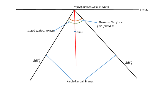
Figure 2: Description of homogeneous Yang-Baxter deformed wedge holography. The presence of homogeneous Yang-Baxter deformation makes it possible to have a non-trivial island surface (solid brown curve) inside the horizon. The green dotted line in the figure corresponds to the black hole horizon. In this figure, we have shown just one part of the wedge holography; the Hartman-Maldacena surface will join the defect located on the other side of wedge holography.

We can see very easily that (83) satisfies the NBC on the branes, i.e., $z^{\prime}(\theta)|_{\theta=\theta_{1},\pi-\theta_{2}}=0$. For $0<\kappa<1$, equation (83) implying $z(\theta)<1$, i.e., $z^{\rm YB\ deformed}<z_{h}$. Since $z(\theta)$ is constant, therefore substituting $z(\theta)$ from (83) into (76), we get the minimal area of the island surface as:

$${\cal A}_{\rm Island}=\int_{\theta_{1}}^{\pi-\theta_{2}}d\theta\sqrt{{\cal G}_{\theta\theta}^{\eta}|_{z=z^{\rm YB\ deformed}}}.$$ (84)

According to Ryu-Takayanagi’s prescription the entanglement entropy of the island surfaces is obtained as [71]:

$$S_{\rm Island}=\frac{2{\cal A}_{\rm Island}}{4G_{N}^{(3)}}=\frac{2\int_{\theta_{1}}^{\pi-\theta_{2}}d\theta\sqrt{{\cal G}_{\theta\theta}^{\eta}|_{z^{\rm YB\ deformed}}}}{4G_{N}^{(3)}}$$

$$=-\frac{2\left(\pi-(\theta_{2}+\theta_{1})\right)\alpha f^{\prime}(z^{\rm YB\ deformed})}{8G_{N}^{(3)}}=2\left(\frac{\left(\pi-(\theta_{2}+\theta_{1})\right)\alpha z^{\rm YB\ deformed}}{4G_{N}^{(3)}}\right)<2S_{\rm thermal}.$$

The factor “2” in the above equation is due to the second island surface contribution from the thermofield double partner. Therefore, we get a non-trivial island surface inside the horizon due to the presence of homogeneous Yang-Baxter deformation whose entanglement entropy is lower than twice of thermal entropy of the black hole.

4.1.3 Page Curve

From subsections 4.1.1 and 4.1.2, we see that the Hartman-Maldacena surface has the linear time dependence (74) and island surface’s entanglement entropy is less than the twice of thermal entropy of the black hole (4.1.2), hence the Page curve without DGP term is obtained as shown in Fig. 3.

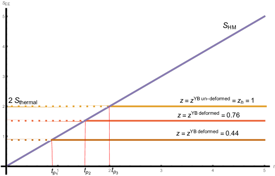
Figure 3: Page curves for various values of $\kappa$.

Fig. 3 has been drawn by dropping the overall factor $\left(\frac{\left(\pi-(\theta_{2}+\theta_{1})\right)\alpha}{4G_{N}^{(3)}}\right)$. This factor is also common in the thermal entropy of the black hole (50). If we consider the numerical value of the aforementioned factor, then this will just scale the Page curves, but the qualitative results will remain the same. To draw the figure, we have taken $\kappa=0,0.2,0.4$ implying $z^{\rm YB\ un-deformed}=z_{h}=1$ and $z^{\rm YB\ deformed}=0.76,0.44$ respectively. The entanglement entropies for $z^{\rm YB\ deformed}=0.76,0.44$ are $S_{\rm Island}=1.52,0.88$ which are less than $2S_{\rm thermal}=2$.

Let us understand the physical meaning of these results. Since $z^{\rm YB\ deformed}<z_{h}$ therefore, extremal surfaces in the presence of homogeneous Yang-Baxter deformation are behind the black hole horizon. See [12, 72] where the island surface was found inside the horizon in non-holographic models. We found this result for the holographic model in this work. Using the entanglement entropies of the island surface and Hartman-Maldacena surface, we obtained the Page curve in wedge holography in the presence of homogeneous Yang-Baxter deformation.

Based on [73, 74, 75], we can say that as soon as the island comes into the picture, one starts recovering the information from the black hole. In Fig. 3, we see that we get different Page curves for different values of $\kappa$, and hence the homogeneous Yang-Baxter deformation is shifting the Page curves. More explicitly, when $\kappa$ increase, then Page curves shift towards earlier time. Therefore, variation of $\kappa$ affects the emergence of islands and information recovery of the Hawking radiation.

4.2 DGP Term and Swampland Criteria in Homogeneous Yang-Baxter Deformed Wedge Holography

In this subsection, we will discuss the effect of including the DGP term on the Karch-Randall branes. As discussed in [27], the Hartman-Maldacena surface entanglement entropy remains same. In the presence of the DGP term, the island surface’s entanglement entropy receives an extra contribution from the boundary of the island surface [27]. In $AdS_{d+1}/CFT_{d}$ correspondence, the same can be expressed as follows:

$$S_{EE}\sim{\rm min}\Biggl{[}{\rm ext}\biggl{(}\int_{\Gamma}d^{d-1}x\sqrt{\gamma}+\int_{\partial\Gamma}d^{d-2}x\sqrt{\sigma}\lambda_{a}\Biggr{)}\Biggr{]},$$ (86)

where $\Gamma$ being the RT surface with induce metric $\gamma$ and boundary of $\Gamma$ ($\partial\Gamma$) has the induced metric $\sigma$.

Recently it has been pointed out that including DGP term on the Karch-Randall brane is non-physical [34, 35]. DGP term can leads to negative entanglement entropy because of negative effective coupling constant of one brane. To have a positive entanglement entropy in the homogeneous Yang-Baxter deformed wedge holography we need to consider $(\theta_{1}+\theta_{2})<\pi$. Another swampland criteria mentioned by authors in [34] is that for any extremal surface if $S_{\rm ext}<S_{\rm thermal}$ then those theories will belong to the swampland.

We obtain the non-trivial island surface in homogeneous Yang-Baxter deformed wedge holography due to the homogeneous Yang-Baxter deformation. We can have positive entanglement entropy for the island surface provided $(\theta_{1}+\theta_{2})<\pi$ and hence we can avoid one of the swampland criteria given in [34]. But in our setup $S_{\rm island}<S_{\rm thermal}$ therefore the second criteria of swampland is unavoidable. Based on the results of [34] we can say that homogeneous Yang-Baxter deformed wedge holography is also the part of swampland.

5 Comment on Inhomogeneous Yang-Baxter Deformed Wedge Holography

One can also construct the wedge holography in inhomogeneous Yang-Baxter deformed AP model by following the steps given below:

• 3D uplift of black hole solution (27): One can construct the $3D$ uplift using the idea of [51]:

  $$ds^{2}=-4F(r)dt^{2}+\frac{dr^{2}}{F(r)}+{\cal G}_{\theta\theta}^{\eta}d\theta^{2},$$ (87)

  where

  $${\cal G}_{\theta\theta}^{\eta}=(1+r)^{2},\ \ \ F(r)=\frac{-1-\eta^{2}\mu+(1-\eta^{2}\mu)\cosh(2\eta r)}{2\eta^{2}}.$$ (88)

• Wedge holography for the bulk (87): We can construct wedge holography for three dimensional bulk (87) similar to our discussion by locating the Karch-Randall branes at constant $\theta$ angles. In this case, two dimensional black holes on Karch-Randall branes have the metric (27).

6 Holographic Complexity in Homogeneous Yang-Baxter Deformed Background

In this section, we compute the holographic complexity of homogeneous Yang-Baxter deformed $AdS_{2}$ using the complexity equals volume proposal [77]. This proposal states that the complexity of holographic dual theory is given by the volume of co-dimension one surface in the bulk. For our case, we have “$AdS_{2}^{\eta}$/deformed SYK” duality, and hence we can write the expression for the holographic complexity as:

$${\cal C}=\frac{{\cal V}}{G_{N}^{(2)}l},$$ (89)

where ${\cal V}$, $G_{N}^{(2)}$, and $l$ are the volume of a one-dimensional surface in two-dimensional bulk, Newton constant in two dimensions, and length scale associated with Yang-Baxter deformed $AdS_{2}$ background respectively.

Let us write the two dimensional metric for homogeneous Yang-Baxter deformed background as:

$$ds^{2}=\frac{{\cal F}_{\eta}(z)}{z^{2}}\Biggl{(}-f(z)dt^{2}+\frac{dz^{2}}{f(z)}\Biggr{)},$$ (90)

where

$${\cal F}_{\eta}(z)=\frac{1}{1-\frac{\kappa^{2}}{z^{2}}};\ \ \ f(z)=1-\frac{z^{2}}{z_{h}^{2}}.$$ (91)

In order to compute holographic complexity, we parametrize the volume slice by “$t(z)$”. The induced metric associated with co-dimension one surface in homogeneous Yang-Baxter deformed $AdS_{2}$ is obatined using (90) and it is written below:

$$ds^{2}|_{\gamma}=\frac{{\cal F}_{\eta}(z)}{z^{2}}\Biggl{(}-f(z)t^{\prime}(z)^{2}+\frac{1}{f(z)}\Biggr{)}dz^{2}.$$ (92)

Using (92), the volume of co-dimension one surface is obtained as:

$${\cal V}=\int dz{\cal L}\left(z,t^{\prime}(z)\right)=\int dz\left(\frac{\sqrt{{\cal F}_{\eta}(z)}\sqrt{\frac{1}{f(z)}-f(z)t^{\prime}(z)^{2}}}{z}\right).$$ (93)

Since there is no explicit $t(z)$ dependence in Lagrangian of (93) therefore energy will be conserved (say $E$), and is given as below:

$$E=-\frac{\partial{\cal L}\left(z,t^{\prime}(z)\right)}{\partial t^{\prime}(z)}=\frac{f(z)\sqrt{{\cal F}_{\eta}(z)}t^{\prime}(z)}{z\sqrt{\frac{1}{f(z)}-f(z)t^{\prime}(z)^{2}}}.$$ (94)

On solving the above equation for $t^{\prime}(z)$, we obtained:

$$t^{\prime}(z)=\frac{Ez}{f(z)\sqrt{E^{2}z^{2}+f(z){\cal F}_{\eta}(z)}}.$$ (95)

We can invert the above equation to get:

$$z^{\prime}(t)\equiv\frac{dz}{dt}=\frac{f(z)\sqrt{E^{2}z^{2}+f(z){\cal F}_{\eta}(z)}}{Ez}.$$ (96)

At the turning point $dz/dt|_{z=z_{t}}=0$, and substituting $f(z)$, ${\cal F}_{\eta}(z)$ from (91) into (96), turning point from (96) is obtained as:

$$z_{t}=\frac{{z_{h}}\sqrt{1-E^{2}\kappa^{2}}}{\sqrt{1-E^{2}{z_{h}}^{2}}}$$ (97)

Now substituting $t^{\prime}(z)$ from (95) into the action (93) and utilizing $f(z)$, ${\cal F}_{\eta}(z)$ from (91), we obtained the on-shell volume as:

$${\cal V}=\int_{z_{B}}^{z_{t}}{\cal L}=\int_{z_{B}}^{z_{t}}\frac{dz}{z}\left(\sqrt{\frac{z^{2}}{z^{2}-\kappa^{2}}}\sqrt{\frac{{z_{h}}^{2}}{{z_{h}}^{2}\left(1-E^{2}\kappa^{2}\right)+z^{2}\left(E^{2}{z_{h}}^{2}-1\right)}}\right).$$ (98)

Utilizing (91) and (95), we obtained the boundary time in the form of following integral:

$$t(z_{B})=t_{b}=-\int_{z_{B}}^{z_{t}}dz\left(\frac{Ez}{\left(1-\frac{z^{2}}{{z_{h}}^{2}}\right)\sqrt{E^{2}z^{2}+\frac{1-\frac{z^{2}}{{z_{h}}^{2}}}{1-\frac{\kappa^{2}}{z^{2}}}}}\right).$$ (99)

At late times, $E$ reaches a critical value, “$E_{\rm crit}$” which can be obtained by extremization of $E$ with respect to $z_{t}$ using (97) as follows:

$$\frac{dE}{dz_{t}}=-\frac{\sqrt{1-E^{2}\kappa^{2}}\left(1-E^{2}{z_{h}}^{2}\right)^{3/2}}{E{z_{h}}\left(\kappa^{2}-{z_{h}}^{2}\right)}.$$ (100)

Hence, extrimation of $E$ $\left(\frac{dE}{dz_{t}}|_{E=E_{\rm crit}}=0\right)$ leads to:

$$E_{\rm crit}=\frac{1}{z_{h}}.$$ (101)

Substituting $E_{\rm crit}$ from (101) into (98) and using the definition of complexity as given in (89), we obtained the complexity growth at late times after differentiating obtained complexity with respect to boundary time ($t_{b}$) as given below:

$${\frac{d{\cal C}}{dt_{b}}}\Biggl{|}_{t_{b}\rightarrow\infty}=\frac{\phi^{\rm YB}}{G_{N}^{(2)}lz_{h}}$$ (102)

where dilaton, $\phi^{\rm YB}={\sqrt{{\cal G}_{\theta\theta}^{\eta}}}|_{z=z_{h}}$, captures information about the transverse space. This can be understood from appendix B. Utilizing the results obtained in appendix A for the Hawking temperature (107), we see that complexity growth at late times (102) simplified as:

$${\frac{d{\cal C}}{dt_{b}}}\Biggl{|}_{t_{b}\rightarrow\infty}=\frac{\phi^{\rm YB}}{G_{N}^{(2)}lz_{h}}=\frac{8\pi S_{\rm YBJT}T_{H}}{l},$$ (103)

where $S_{\rm YBJT}=\frac{\phi^{\rm YB}}{4G_{N}^{(2)}}$. Therefore, we see that complexity growth in the presence of Yang-Baxter deformation is proportional to product of the the Bekenstein-Hawking entropy and Hawking temperature of two dimensional black hole.

7 Conclusion and Discussion

In this paper, we have constructed the wedge holography in homogeneous Yang-Baxter deformed $AdS_{3}$ background. The same has been done by considering the two Karch-Randall branes located at $\theta=\theta_{1,2}$ and the homogeneous Yang-Baxter deformed bulk $AdS_{3}$ metric that satisfies Neumann boundary condition on the branes. In our case, the defect that connects the two Karch-Randall branes can be identified as a “deformed SYK model”. In this way, we proposed the co-dimension two holography for the “deformed SYK model”. In other words, this is the, “duality between a homogeneous Yang-Baxter deformed $AdS_{3}$ bulk and deformed SYK model living at the defect”.

Let us summarise the key results of the paper.

• In this setup, the non-conformal boundary of the homogeneous Yang-Baxter deformed $AdS_{3}$ bulk is located at the holographic screen placed at $z=z_{B}$. Hence, the defect is also located at the holographic screen in this setup as shown in Fig. 2. In homogeneous Yang-Baxter deformed wedge holography, two-dimensional field theory is dual to three-dimensional bulk located at the holographic screen which we termed as “Holographic Screen Non-Conformal Field Theory (HSNCFT)”. Since we have homogeneous Yang-Baxter $AdS_{2}$ on the Karch-Randall branes and hence the deformed SYK model is living at defect situated at the holographic screen because of “$AdS_{2}^{\eta}$/deformed SYK” duality. Overall, deformed SYK model living at the defect is dual to three-dimensional bulk.

• According to the wedge holography, the only possible extremal surface is the black hole horizon [25]. The authors in [27, 29, 30] obtained non-trivial island surface with entanglement entropy lower than the thermal entropy of the black hole by including the DGP term on the Karch-Randall branes. This possibility has been ruled out by the swampland criteria discussed in [34, 35].

• We used the homogeneous Yang-Baxter deformed wedge holography to obtain the Page curve of the black hole and obtained the usual Page curve without DGP term in the presence of homogeneous Yang-Baxter deformation in contrast to the flat Page curve as obtained in [25, 27, 29]. The homogeneous Yang-Baxter deformation is the reason for the existence of non-trivial island surface inside the black hole horizon.

Let us compare our results with the literature. In [25], authors argued that we could not get the Page curve in usual wedge holography because the only possible extremal surface is the black hole horizon. In this paper, we showed that there exists a non-trivial island surface inside the horizon in our case if we include the homogeneous Yang-Baxter deformation in our setup. If we switch off the homogeneous Yang-Baxter deformation, then the extremal surface is the black hole horizon similar to [25].

We also compute the holographic complexity of homogeneous Yang-Baxter deformed $AdS_{2}$ background using the complexity equals volume proposal [77], and find that complexity growth at late times is proportional to the product of Bekenstein-Hawking entropy and temperature of black hole in Yang-Baxter deformed $AdS_{2}$ background. Without Yang-Baxter deformation, our results reduce to ones obtained in [78].

In this paper, we restrict ourselves to the homogeneous Yang-Baxter deformed background. Future direction could be the construction of wedge holography and study of holographic complexity in inhomogeneous Yang-Baxter deformed background [47].

Appendix A Hawking Temperature of Black Hole in Homogeneous Yang-Baxter Deformed $AdS_{2}$ Background

Black hole solution is given as:

$$ds^{2}_{\eta}=-g_{tt}(z)dt^{2}+g_{zz}(z)dz^{2}={\cal F}_{\eta}(z)\Biggl{(}\frac{-f(z)dt^{2}+\frac{dz^{2}}{f(z)}}{z^{2}}\Biggr{)},$$ (104)

where

$${\cal F}_{\eta}(z)=\frac{1}{1-\frac{\kappa^{2}}{z^{2}}},\ \ f(z)=1-\frac{z^{2}}{z_{h}^{2}}\hskip 2.84526pt.$$ (105)

We can calculate the Hawking temperature using the following formula [79]:

$$T_{H}=\frac{\kappa}{2\pi}=\Biggl{|}Limit_{z\rightarrow z_{h}}\frac{\partial_{z}g_{tt}(z)}{4\pi\sqrt{g_{tt}(z)g_{zz}(z)}}\Biggr{|}.$$ (106)

Using (104) and (105), we obtained the Hawking temperature after simplification of (106) as follows:

$$T_{H}=\frac{1}{2\pi z_{h}}.$$ (107)

Appendix B Dimensional Reduction from $3D$ to $2D$

Three dimensional action is given by [51]:

$$S_{\rm 3D}=\frac{1}{16\pi G_{N}^{(3)}}\Biggl{(}\int_{M}d^{3}x\sqrt{-g^{(3)}}(R^{(3)}-2\Lambda)\Biggr{)},$$ (108)

Upon dimensional reduction along $\theta$, using the ansatz: $ds^{2}=g^{(3)}_{MN}dx^{M}dx^{N}=h^{(2)}_{ij}dx^{i}dx^{j}+{\cal G}_{\theta\theta}^{\eta}d\theta^{2}\equiv h^{(2)}_{ij}dx^{i}dx^{j}+\left(\phi^{\rm YB}\right)^{2}d\theta^{2}$, three dimensional Ricci scalar is obtained as: $R^{(3)}=R+\phi_{\eta}$ (where $R$ is two dimensional Ricci scalar), and hence action (108) reduces to:

$$\hskip-21.68121ptS_{\rm 2D}=\frac{\Sigma_{I}}{16\pi G_{N}^{(3)}}\Biggl{(}\int d^{2}x\sqrt{-h^{(2)}}\phi^{\rm YB}(R+\phi_{\eta}-2\Lambda)\Biggr{)}$$

$$\equiv\frac{1}{16\pi G_{N}^{(2)}}\Biggl{(}\int d^{2}x\sqrt{-h^{(2)}}\phi^{\rm YB}(R+\phi_{\eta}-2\Lambda)\Biggr{)},$$ (109)

where $\Sigma_{I}$ being the volume of compact space and

$$\frac{1}{G_{N}^{(2)}}=\frac{\Sigma_{I}}{G_{N}^{(3)}},$$

$$\phi^{\eta}=\frac{z^{2}\left(\left(\partial_{t}{\cal G}_{\theta\theta}^{\eta}\right)^{2}-\left(\partial_{z}{\cal G}_{\theta\theta}^{\eta}\right)^{2}+2{\cal G}_{\theta\theta}^{\eta}\left(-\partial_{t}^{2}+\partial_{z}^{2}\right){\cal G}_{\theta\theta}^{\eta}\right)}{4{\cal F}_{\eta}(z)\left({\cal G}_{\theta\theta}^{\eta}\right)^{2}}.$$ (110)

It has been shown in [51] that $\sqrt{{\cal G}_{\theta\theta}^{\eta}}\phi_{\eta}=\phi^{\rm YB}\phi_{\eta}=-U\left(\Phi_{\eta}^{2}\right)$, i.e. one obtains the dilaton potential of [47]. Hence,

$$S_{\rm 2D}=\frac{1}{16\pi G_{N}^{(2)}}\Biggl{[}\int d^{2}x\sqrt{-h^{(2)}}\Biggl{(}\phi^{\rm YB}(R-2\Lambda)-U\left(\Phi_{\eta}^{2}\right)\Biggr{)}\Biggr{]}.$$ (111)

Variation of (111) with respect to $h_{ij}$ leads to the Einstein’s equation with negative cosmological constant in two dimensions:

$$R_{ij}-\frac{R[h_{ij}]}{2}h_{ij}+\Lambda h_{ij}=0.$$ (112)

References

- [1] J. M. Maldacena, The Large N limit of superconformal field theories and supergravity, Int. J. Theor. Phys. 38, 1113-1133 (1999) [arXiv:hep-th/9711200].
- [2] S.W. Hawking, Particle Creation by Black Holes, Commun. Math. Phys. 43, 199 (1975) Erratum: [Commun. Math. Phys. 46, 206 (1976)].
- [3] S.W. Hawking, Breakdown of Predictability in Gravitational Collapse, Phys. Rev. D 14 (1976) 2460-2473.
- [4] D.N. Page, Information in Black Hole Radiation, Phys.Rev.Lett. 71 (1993) 3743-3746 [arXiv:hep-th/9306083 [hep-th]].
- [5] A. Almheiri, R. Mahajan, J. Maldacena and Y. Zhao, The Page curve of Hawking radiation from semiclassical geometry, JHEP 03 (2020) 143 [1908.10996].
- [6] T. J. Hollowood, S. P. Kumar, Islands and Page curves for evaporating black holes in JT gravity, J. High Energ. Phys. 2020, 94 (2020)[arXiv:2004.14944[hep-th]].
- [7] T.J. Hollowood, S. P. Kumar and A. Legramandi, Hawking radiation correlations of evaporating black holes in JT gravity, J.Phys.A 53 (2020) 47, 475401 [arXiv:2007.04877[hep-th]].
- [8] T.J. Hollowood, S. P. Kumar, A. Legramandi and N. Talwar, Islands in the stream of Hawking radiation, J. High Energ. Phys. 2021, 67 (2021) [arXiv:2104.00052 [hep-th]].
- [9] T.J. Hollowood, S. P. Kumar, A. Legramandi and N. Talwar, Ephemeral islands, plunging quantum extremal surfaces and BCFT channels, J. High Energ. Phys. 2022, 78 (2022) [arXiv: 2109.01895[hep-th]].
- [10] T.J. Hollowood, S. P. Kumar, A. Legramandi and N. Talwar, Grey-body factors, irreversibility and multiple island saddles, J. High Energ. Phys. 2022, 110 (2022) [arXiv:2111.02248 [hep-th]].
- [11] Z. Gyongyosi, T.J. Hollowood, S.P. Kumar, A. Legramandi and N. Talwar, Black Hole Information Recovery in JT Gravity, J. High Energ. Phys. 2023, 139 (2023) [arXiv:2209.11774 [hep-th]].
- [12] G. Yadav and N. Joshi, Cosmological and black hole islands in multi-event horizon spacetimes, Phys. Rev. D 107, 026009 (2023) [arXiv:2210.00331[hep-th]].
- [13] G. Yadav, Page Curves of Reissner-Nordström Black Hole in HD Gravity, Eur. Phys. J. C 82 (2022) 904 [arXiv:2204.11882[hep-th]].
- [14] K. Goswami and K. Narayan, Small Schwarzschild de Sitter black holes, quantum extremal surfaces and islands, JHEP 10 (2022) 031 [arXiv:2207.10724[hep-th]].
- [15] F. Omidi, Entropy of Hawking radiation for two-sided hyperscaling violating black branes, JHEP 04, 022 (2022) [arXiv:2112.05890 [hep-th]].
- [16] G. Yadav and A. Misra, Entanglement entropy and Page curve from the M-theory dual of thermal QCD above at intermediate coupling, Phys. Rev. D 107, 106015 (2023) [arXiv:2207.04048[hep-th]].
- [17] C. J. Chou, H. B. Lao and Y. Yang, Page curve of effective Hawking radiation, Phys. Rev. D 106, no.6, 066008 (2022) [arXiv:2111.14551 [hep-th]].
- [18] C. J. Chou, H. B. Lao and Y. Yang, Page Curve of AdS-Vaidya Model for Evaporating Black Holes, [arXiv:2306.16744 [hep-th]].
- [19] P. J. Hu and R. X. Miao, Effective action, spectrum and first law of wedge holography, JHEP 03 (2022)145 [arXiv:2201.02014].
- [20] H. Geng, A. Karch, C. P. Pardavila, S. Raju, L. Randall, M. Riojas, and S. Shashi, Jackiw-Teitelboim Gravity from the Karch-Randall Braneworld, Phys.Rev.Lett. 129 (2022) 23, 231601 [arXiv:2206.04695].
- [21] N. Ogawa, T. Takayanagi, T. Tsuda and T. Waki, Wedge Holography in Flat Space and Celestial Holography, [arXiv:2207.06735].
- [22] T. Hartman and J. Maldacena, Time Evolution of Entanglement Entropy from Black Hole Interiors, JHEP 05 (2013) 014 [arXiv:1303.1080[hep-th]].
- [23] O. Aharony, O. DeWolfe, D.Z. Freedman and A. Karch, Defect conformal field theory and locally localized gravity, JHEP 07 (2003) 030 [hep-th/0303249].
- [24] H. Geng and A. Karch, Massive islands, JHEP 09 (2020) 121 [arXiv:2006.02438[hep-th]].
- [25] H. Geng, A. Karch, C. P. Pardavila, S. Raju and L. Randall, Information Transfer with a Gravitating Bath, SciPost Phys. 10 (2021) 5, 103 [arXiv:2012.04671[hep-th]].
- [26] H. Geng, A. Karch, C. P. Pardavila, S. Raju and L. Randall, Inconsistency of islands in theories with long-range gravity, JHEP 01 (2022) 182 [arXiv:2107.03390[hep-th]].
- [27] R. X. Miao, Massless Entanglement Island in Wedge Holography, [arXiv:2212.07645[hep-th]].
- [28] K. Ghosh and C. Krishnan, Dirichlet baths and the not-so-fine-grained Page curve, JHEP 08 (2021) 119 [arXiv:2103.17253[hep-th]].
- [29] R. X. Miao, Entanglement Island and Page Curve in Wedge Holography, JHEP 03 (2023) 214 [arXiv:2301.06285[hep-th]].
- [30] C. P. Pardavila, Entropy of Radiation with Dynamical Gravity, arXiv:2302.04279[hep-th].
- [31] D. Li and R. X. Miao, Massless Entanglement Islands in Cone Holography, arXiv:2303.10958[hep-th].
- [32] G. R. Dvali, G. Gabadadze and M. Porrati, 4D gravity on a brane in 5D Minkowski space, Phys. Lett. B 485 (2000) 208 [hep-th/0005016].
- [33] C. Vafa, The String landscape and the swampland, [arXiv:hep-th/0509212]; N. Arkani-Hamed, L. Motl, A. Nicolis and C. Vafa, The String landscape, black holes and gravity as the weakest force, JHEP 06 (2007) 060 [arXiv:hep-th/0601001]; H. Ooguri and C. Vafa, On the Geometry of the String Landscape and the Swampland, Nucl. Phys. B 766 (2007) 21 [arXiv:hep-th/0605264].
- [34] H. Geng, A. Karch, C. P. Pardavila, L. Randall, M. Riojas, S. Shashi and M. Youssef, Constraining braneworlds with entanglement entropy, arXiv:2306.15672.
- [35] H. Geng, Entropy, Entanglement Islands and Swampland Bounds in the Karch-Randall Braneworld, arXiv:2306.15671.
- [36] A. Misra and V. Yadav, On -Theory Dual of Large- Thermal QCD-Like Theories up to and -Structure Classification of Underlying Non-Supersymmetric Geometries, to appear in Advances in Theoretical and Mathematical Physics (issue 28.10) [arXiv:2004.07259 [hep-th]].
- [37] G. Yadav, Multiverse in Karch-Randall Braneworld, JHEP 03 (2023) 103 [arXiv:2301.06151[hep-th]].
- [38] T. Matsumoto and K. Yoshida, Yang–Baxter sigma models based on the CYBE, Nucl. Phys. B 893, 287-304 (2015) [arXiv:1501.03665 [hep-th]].
- [39] C. Klimcik, Yang-Baxter sigma models and dS/AdS T duality, JHEP 12, 051 (2002)[arXiv:hep-th/0210095 [hep-th]].
- [40] C. Klimcik, On integrability of the Yang-Baxter sigma-model, J. Math. Phys. 50, 043508 (2009) [arXiv:0802.3518 [hep-th]].
- [41] F. Delduc, M. Magro and B. Vicedo, On classical -deformations of integrable sigma-models, JHEP 11, 192 (2013) [arXiv:1308.3581 [hep-th]].
- [42] J. Pal, H. Rathi, A. Lala and D. Roychowdhury, Non-chaotic dynamics for Yang-Baxter deformed superstrings [arXiv:2208.09599 [hep-th]].
- [43] D. Roychowdhury, Analytic integrability for strings on and deformed backgrounds, JHEP 10 (2017) 056 [arXiv:1707.07172[hep-th]].
- [44] D. Roychowdhury, Probing deformed backgrounds with Dp branes, Phys. Lett. B 778 (2018) 167–173 [arXiv:1706.02625[hep-th]].
- [45] A. Banerjee, A. Bhattacharyya and D. Roychowdhury, Fast spinning strings on deformed , JHEP 02 (2018) 035 [arXiv:1711.07963[hep-th]].
- [46] D. Roychowdhury, On pp wave limit for deformed superstrings, JHEP 05 (2018) 018 [arXiv:1801.07680[hep-th]].
- [47] H. Kyono, S. Okumura and K. Yoshida, Deformations of the Almheiri-Polchinski model, JHEP 03, 173 (2017) [arXiv:1701.06340 [hep-th]].
- [48] H. Kyono, S. Okumura and K. Yoshida, Comments on 2D dilaton gravity system with a hyperbolic dilaton potential, Nucl. Phys. B 923, 126-143 (2017) [arXiv:1704.07410 [hep-th]].
- [49] S. Okumura and K. Yoshida, Weyl transformation and regular solutions in a deformed Jackiw–Teitelboim model, Nucl. Phys. B 933, 234-247 (2018) [arXiv:1801.10537 [hep-th]].
- [50] A. Almheiri and J. Polchinski, Models of AdS2 backreaction and holography, JHEP 11, 014 (2015) [arXiv:1402.6334 [hep-th]].
- [51] A. Lala and D. Roychowdhury, SYK/AdS duality with Yang-Baxter deformations, JHEP 12 (2018) 073 [arXiv:1808.08380[hep-th]].
- [52] R. M. Wald, Black Hole Entropy is Noether Charge, Phys. Rev. D 48, 3427 (1993) [arXiv:gr-qc/9307038].
- [53] V. Iyer and R. M. Wald, Some Propeties of Noether Charge and a Proposal for Dynamical Black Hole Entropy, Phys. Rev. D 50, 846 (1994) [arXiv:gr-qc/9403028].
- [54] R. X. Miao, An Exact Construction of Codimension two Holography, JHEP 01, 150 (2021) [arXiv:2009.06263 [hep-th]].
- [55] I. Akal, Y. Kusuki, T. Takayanagi and Z. Wei, Codimension two holography for wedges, Phys. Rev. D 102, no.12, 126007 (2020) [arXiv:2007.06800 [hep-th]].
- [56] D. Roychowdhury, Stringy correlations on deformed , JHEP 03, 043 (2017) [arXiv:1702.01405 [hep-th]].
- [57] C. Krishnan, V. Patil and J. Pereira, Page Curve and the Information Paradox in Flat Space, arXiv:2005.02993.
- [58] A. Karch and L. Randall, Locally localized gravity, JHEP 05 (2001) 008 [hep-th/0011156].
- [59] A. Karch and L. Randall, Open and closed string interpretation of SUSY CFT’s on branes with boundaries, JHEP 06 (2001) 063 [hep-th/0105132].
- [60] S. Sachdev and J. Ye, Gapless spin fluid ground state in a random, quantum Heisenberg magnet, Phys. Rev. Lett. 70, 3339 (1993) [arXiv:cond-mat/9212030 [cond-mat]].
- [61] A.Kitaev.2015. A simple model of quantum holography, talk given at KITP strings seminar and Entanglement program, February 12, April 7, and May 27, Santa Barbara, U.S.A.
- [62] J. Maldacena and D. Stanford, Remarks on the Sachdev-Ye-Kitaev model, Phys. Rev. D 94, no.10, 106002 (2016) [arXiv:1604.07818 [hep-th]].
- [63] J. Polchinski and V. Rosenhaus, The Spectrum in the Sachdev-Ye-Kitaev Model, JHEP 04, 001 (2016) [arXiv:1601.06768 [hep-th]].
- [64] K. Jensen, Chaos in AdS2 Holography, Phys. Rev. Lett. 117, no.11, 111601 (2016) [arXiv:1605.06098 [hep-th]].
- [65] S. R. Das, A. Jevicki and K. Suzuki, Three Dimensional View of the SYK/AdS Duality, JHEP 09, 017 (2017) [arXiv:1704.07208 [hep-th]].
- [66] S. R. Das, A. Ghosh, A. Jevicki and K. Suzuki,Three Dimensional View of Arbitrary SYK models, JHEP 02, 162 (2018) [arXiv:1711.09839 [hep-th]].
- [67] D. Roychowdhury, Holographic derivation of SYK spectrum with Yang-Baxter shift, Phys. Lett. B 797, 134818 (2019) [arXiv:1810.09404 [hep-th]].
- [68] J. Maldacena, D. Stanford and Z. Yang, Conformal symmetry and its breaking in two dimensional Nearly Anti-de-Sitter space, PTEP 2016, no.12, 12C104 (2016) [arXiv:1606.01857 [hep-th]].
- [69] A. Goel, V. Narovlansky and H. Verlinde, Semiclassical geometry in double-scaled SYK, [arXiv:2301.05732 [hep-th]].
- [70] Q. L. Hu, D. Li, R. X. Miao and Y. Q. Zhao, AdS/BCFT and Island for curvature-squared gravity, JHEP 09 (2022) 037 [arXiv:2202.03304[hep-th]].
- [71] S. Ryu, T. Takayanagi, Holographic Derivation of Entanglement Entropy from AdS/CFT, Phys. Rev. Lett. 96, 181602 (2006) [arXiv:hep-th/0603001].
- [72] W. C. Gan, D. H. Du and F. W. Shu, Island and Page curve for one-sided asymptotically flat black hole, JHEP 07 (2022) 020 [arXiv:2203.06310 [hep-th]].
- [73] P. Hayden and J. Preskill, Black holes as mirrors: quantum information in random subsystems JHEP, 0709:120,2007 [arXiv:0708.4025[hep-th]].
- [74] Y. Sekino and L. Susskind, Fast Scramblers, JHEP 0810:065,2008 [arXiv:0808.2096[hep-th]].
- [75] G. Penington, Entanglement Wedge Reconstruction and the Information Paradox, [arXiv:1905.08255[hep-th]].
- [76] A. Anand, Page Curve and Island in EGB Gravity, [arXiv:2205.13785[hep-th]].
- [77] D. Stanford and L. Susskind, Complexity and shock wave geometries, Phys. Rev. D 90, 126007 (2014) [arXiv:1406.2678[hep-th]].
- [78] A. Bhattacharya, A. Bhattacharyya and A. K. Patra, Holographic complexity of Jackiw-Teitelboim gravity from Karch-Randall braneworld, arXiv:2304.09909[hep-th].
- [79] G. Yadav, Deconfinement temperature of rotating QGP at intermediate coupling from M-theory, Phys. Lett. B 841, 137925 (2023) [arXiv:2203.11959 [hep-th]].