Riemann zeros as quantized energies of scattering with impurities

Abstract

We construct a physical model of a single particle interacting with impurities spread on a circle, where the quantized energies coming from a Bethe Ansatz equation correspond to the non-trivial zeros of the Riemann $\zeta$-function.

I Introduction

If the Riemann Hypothesis has fascinated mathematicians for decades (see Edwards ; Borwein ; Conrey ), it has also fascinated theoretical physicists for quite a long time (for a review up to 2011, see for instance Schumayer ). The idea that a remarkable mathematical property may be understood from the simple and elegant requirements of a physical system is too appealing to pass up. “Understanding” is obviously different from “proving” but it may nevertheless be the first promising step toward a more rigorous approach. It is precisely with such a “theoretical physicist attitude” that we approach the famous problem of the alignment of all zeros of the Riemann zeta function $\zeta(s)$ along the axis ${\mathbb{R}e}\,s=1/2$.

One of the most prominent physical proposals is probably the Hilbert-Pólya idea: it turns the problem of establishing the validity of the Riemann Hypothesis into the existence of a single particle quantum Hamiltonian whose eigenvalues are equal to the ordinates of zeros on the critical line. This has been pursued in several relevant papers, such as BerryK ; BerryK2 ; Sierra ; Sredincki ; Bender . In that approach, one searches for a quantum Hamiltonian where the bound state energies are the non-trivial Riemann zeros on the critical line. A different approach, based on statistical physics where random walks play an essential role, has also been pursued MLRW . The aleatory nature of the problem arises from the pseudo-randomness of the Möbius coefficients evaluated on primes and this property can be checked with astonishing accuracy MLRW . Up to logarithmic corrections, in this statistical physics approach the validity of the Riemann Hypothesis can be easily understood in physical terms from the universality of the critical exponent $1/2$ of the random walk. The zeta function has also been employed in describing scattering amplitudes in quantum mechanics Gutzwiller and quantum field theory Remmen .

In this article we define a new approach, formulated as a quantum mechanical scattering problem rather than a bound state problem. Our proposal radically differs from those previously mentioned Gutzwiller ; Remmen for, in the model we construct, we have a quantization condition for the energies of the system which comes from a Bethe Ansatz equation. The solutions of this Bethe Ansatz equation are exactly the Riemann zeros. This relies on both the functional equation satisfied by $\zeta(s)$ and its Euler product formula in an essential manner.

II Bethe ansatz equation for impurities on a circle: The most general case

Consider a single particle of momentum $p$ moving on a circle of circumference $R$ without any internal degree of freedom. Such a particle has a dispersion relation $E(p)$ where $E$ is the energy of the particle, typically relativistic or non-relativistic. For generality we leave this dispersion relation unspecified for this section. We suppose there are $N$ stationary impurities spread out on the circle, with no particular location, except that they are separated, and label them $j=1,2,\ldots N$, as illustrated in Figure 1. When the particle scatters through a single impurity, there is generally both a transmission and reflection amplitude. We assume there is no reflection, namely the scattering is purely transmitting. There are many known examples of purely transmitting relativistic theories DMS ; KonikLeClair ; Corrigan , in fact infinitely many that are integrable, and there are also non-relativistic examples of reflectionless potentials NonRelativistic0 ; NonRelativistic . To each impurity labeled $j$ we associate a transmission S-matrix $S_{j}(p)$, which by unitarity, is a phase

$$S_{j}(p)=e^{i\phi_{j}(p)}\,\,\,.$$ (1)

Due to the purely transmitting property, the scattering matrix for 2 impurities $j,j^{\prime}$ is simply $S_{j}(p)S_{j^{\prime}}(p)$, and so on.

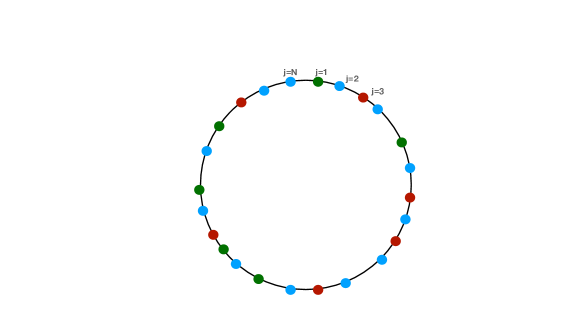
Figure 1: Impurities on a circle labeled $j=1,2,...,N$. Different colors denote different scattering phases. There are not enough colors to represent the scattering problem considered here.

As the particle moves around the circle, it scatters through each impurity and, coming back to its original position, the matching requirement for its wavefunction leads to the quantization condition of its momentum $p$ expressed by

$$e^{ipR}\,\prod_{j=1}^{N}S_{j}(p)=\pm 1\,\,\,,$$ (2)

where $+1,-1$ corresponds to bosons, fermions respectively (see, for instance MussardoBook and references therein). If we take the particles to be fermions, we end up with the Bethe-ansatz equation yangyang ; ZamTBA

$$p_{n}R+\sum_{j=1}^{N}\phi_{j}(p_{n})=2\pi\,(n-\tfrac{1}{2})\,,$$ (3)

for some integer $n$. Then the quantized energies of the system are $E_{n}=E(p_{n})$.

There are several physical applications of this general formula: let us mention, for instance, that if the scattering phases $\phi_{j}$ are random, this is essentially a problem of electrons in a random potential in $1$ dimension and related to Anderson localization.

III Scattering problem that asymptotically yields the Riemann zeros on the critical line

In this section we construct a physical scattering problem where the $E_{n}$ of the last section are asymptotically the Riemann zeros on the critical line. We first specify the dispersion relation $E(p)$ for the free particle between impurities. Let us take

$$p=E\log(E/\hbar\omega)/v$$ (4)

where $v$ is a speed, such as the speed of light, and $\omega$ is a fixed frequency with units of inverse time. Without the $\log E$ term, this is a relativistic dispersion relation for a massless particle where $v$ is the speed of light. We henceforth set $\hbar=1$. Without loss of generality we can redefine $v,\omega$ such that $p$ and $E$ are dimensionless, and

$$p=E\,\log\left(\dfrac{E}{2\pi e}\right)$$ (5)

where $e$ is the Euler number, i.e. $1=\log e$. Note that $p$ is a monotonic function of $E$. Hence, the above dispersion relation can be inverted:

$$E(p)=\dfrac{p}{W(p/2\pi e)}$$ (6)

where $W$ is the Lambert $W$ function. For large $x$, $W(x)=\log x-\log\log x+....$. Thus for large $p$,

$$E(p)\approx\dfrac{p}{\log p}.$$ (7)

Note that as $p\to 0$, $E(p)\to 0$, which is the natural limit of this quantity, based on physics.

Let us now specify the scattering phases. We suppose that the transmission S-matrices are more easily expressed in terms of the energy $E$ rather than the momentum $p$. To each impurity $j$ we associate a positive real number $q_{j}$:

$$S_{j}(E)=\dfrac{q_{j}^{1/2+\delta}-e^{iE\log q_{j}}}{q_{j}^{1/2+\delta}-e^{-iE\log q_{j}}},$$ (8)

where $\delta$ is a positive real number which we will eventually take to $\delta\to 0^{+}$ . Note that at zero energy $S_{j}(0)=1$, which is again physically reasonable, since there should be no scattering if the particle has zero momentum. This implies that the scattering phases are

$$\phi_{j}(E)=-2\,\Im\log\left(1-\dfrac{e^{-iE\log q_{j}}}{q_{j}^{1/2+\delta}}\right)\,.$$ (9)

Whether there exists a Hamiltonian that leads to these S-matrices we leave as a problem for further study. Hereafter we take the attitude that a theory is defined by its S-matrices and there are well known problems where the theory is defined through its S-matrix while the hamiltonian remains unknown (see, for instance MussardoBook ). Without loss of generality, we set $R=1$, since $R$ with physical dimension of length can be absorbed into various constants above, such as $v,\omega$. The Bethe equation (3) now reads

$$\dfrac{E_{n}}{2}\log\left(\dfrac{E_{n}}{2\pi e}\right)-\sum_{j=1}^{N}\Im\log\left(1-\dfrac{e^{-iE_{n}\log q_{j}}}{q_{j}^{1/2+\delta}}\right)=(n-\tfrac{3}{2})\pi$$ (10)

where we have shifted for later convenience $n$ by $-1$.

So far, this is still quite general, and there are no convergence issues if $N$ is finite. For our purposes we chose to take $q_{j}$ to be the $j$-th prime number, i.e. $q_{j}=\mathfrak{p}_{j}$ where $\{\mathfrak{p}_{1},\mathfrak{p}_{2},\mathfrak{p}_{3},\ldots\}=\{2,3,5,\ldots\}$. Let’s mention, en passant, that another interesting choice would be to take $q_{j}$ as any random integer number between two consecutive primes Grosswald , although we address the study of this case somewhere else LM2 . The impurities do not have to be ordered in any specific manner. Now, if $\delta>1/2$ the sum over scattering phases in (10) converges as $N\to\infty$ and, when $\mathfrak{p}_{j}$ is the $j$-th prime number, the equation becomes

$$\dfrac{E_{n}}{2}\log\left(\dfrac{E_{n}}{2\pi e}\right)+{\rm arg}\,\zeta(\tfrac{1}{2}+\delta+iE_{n})=(n-\tfrac{3}{2})\pi$$ (11)

where $\zeta(s)$ is the Riemann zeta function, defined both as a Dirichlet series on the integers $n$ and an infinite product on the primes $\mathfrak{p}$

$$\zeta(s)\,=\,\sum_{n=1}^{\infty}\dfrac{1}{n^{s}}\,=\,\prod_{j=1}^{\infty}\dfrac{1}{1-\dfrac{1}{\mathfrak{p}_{j}^{s}}}\,\,\,~{}~{}~{}~{}~{}(\Re(s)>1).$$ (12)

It is important to remark that ${\rm arg}\,z$ in (11) is the true phase that keeps track of branches, and not ${\rm Arg}\,z={\rm arg}\,z~{}{\rm mod}~{}2\pi$, where ${\rm Arg}$ is the principle branch with $-\pi<{\rm Arg}<\pi$. Although each term in (10) is an ${\rm Arg}$ by the nature of the scattering phase, the sum of ${\rm Arg}$’s can accumulate, i.e. the sum of ${\rm Arg}$’s is not ${\rm Arg}$ of the sum, but ${\rm arg}$ of the sum. See also Section V for more specific remarks.

When $\delta>1/2$, there is a unique solution to the equation (11) for every $n$ since for $E$ sufficiently large, i.e. $E>E_{0}$ (and it is sufficient to take $E_{0}\sim 10$), the left hand side of the equation is a monotonically increasing function of $E_{n}$. In order to get inside the critical strip to the right of the critical line requires $0<\delta<1/2$. In this case, there are essentially three options to deal with this:

• First, one can simply take a finite number $N$ of impurities, so there are no convergence issues. It is known that a truncated Euler product for finite $N$ can be a good approximation to $\zeta$ if the truncation is well chosen, as we will explain below.

• The second option is to just declare that $\zeta(s)$ in (11) is the standard analytic continuation presented by Riemann.

• The third is to replace the $\zeta$ function by one based on a non-principal Dirichlet character $\chi$, where the Euler product takes the form

  $$L(s,\chi)=\sum_{n}\dfrac{\chi(n)}{n^{s}}=\prod_{j=1}^{\infty}\left(1-\dfrac{\chi(\mathfrak{p}_{j})}{\mathfrak{p}_{j}^{s}}\right)^{-1},~{}~{}~{}~{}~{}\Re(s)>1.$$ (13)

  This function has no pole at $s=1$ thus it is possible the Euler product converges to the right of the critical line. In fact it was argued that this is indeed the case due to a random walk property of the sum $\sum_{\mathfrak{p}}\chi(\mathfrak{p})$ arising from the pseudo-randomness of the primes LMDirichlet .

There are an infinite number of potentially interesting scattering problems based on these generalized zeta functions, but for simplicity here we will only consider the first two options.

As $\delta\to 0^{+}$, the quantized energies asymptotically approach the Riemann zeros on the critical line. The equation (11) was first proposed in Electrostatic and, as a matter of fact, it is not very asymptotic at all. For the lowest zero at $n=1$, with $\delta=0.0001$, one finds $E_{1}=14.1347$, which is correct to 6 digits. By systematically reducing $\delta$ one can calculate the Riemann zeros to great accuracy from the exact equation described in the next section, from thousands to even millions of digits for even the lowest zeros FrancaLeClair . In this article we limit the numerics to zeros around the $100$-th for illustration, but very similar results apply to much higher zeros. From (11) we obtain

$$\{E_{100},E_{101},\ldots,E_{104}\}=\{236.524,237.769,239.555,241.049,242.823\}$$ (14)

which are identical to the true Riemann zeros to the number of digits shown. (Here we have also taken $\delta=0.0001$.) If one adopts the prescription of a finite number of impurities, one still obtains good results. For only $N=1000$ impurities, for example, one finds

$$\{E_{100},E_{101},\ldots,E_{104}\}=\{236.521,237.777,238.139,241.057,242.812\}.$$ (15)

IV Scattering problem for the exact Riemann zeros

In this section we explain the phenomenon observed in the last section and refine the model to give the exact Riemann zeros on the critical line. Following standard conventions in analytic number theory, let us define a complex variable $s=\sigma+it$, where based on the above notation $\sigma=\tfrac{1}{2}+\delta$ and $t=E$. We consider zeros on the critical line, which are known to be infinite in number Hardy . Denote the $n$-th zero on the upper critical line as

$$\rho_{n}=\tfrac{1}{2}+it_{n},~{}~{}~{}~{}~{}n=1,2,3,\ldots$$ (16)

where $t_{1}=14.1347..$ is the first zero, and so forth. Labeling them this way, we define below an impurity scattering problem where $E_{n}$ of the previous section become the exact $t_{n}$.

Define a completed $\zeta$ function as follows:

$$\chi(s)=\pi^{-s/2}\Gamma(s/2)\zeta(s),$$ (17)

which satisfies the non-trivial functional equation

$$\chi(1-s)=\chi(s).$$ (18)

Let us now write $\chi(s)$ in terms of a positive, real modulus $|\chi(s)|$ and argument $\theta$:

$$\chi(s)=|\chi(s)|\,e^{i\theta(\sigma,t)},$$ (19)

i.e.

$$\theta(\sigma,t)={\rm arg}\,\chi(\sigma+it).$$ (20)

Again, here it is important that $\theta$ is the true ${\rm arg}$, not ${\rm Arg}={\rm arg}~{}{\rm mod}~{}2\pi$, where ${\rm Arg}$ is the principle branch with $-\pi<{\rm Arg}<\pi$. Obviously

$$\theta(\sigma,t)=\vartheta(\sigma,t)+{\rm arg}\,\zeta(\sigma+it)$$ (21)

where

$$\vartheta(\sigma,t)\equiv{\rm arg}\,\Gamma\left(\tfrac{1}{2}(\sigma+it)\right)-\tfrac{t}{2}\log\pi.$$ (22)

On the critical line $\vartheta(\tfrac{1}{2},t)$ is commonly referred to as the Riemann-Siegel $\vartheta$ function. Below, if it is implicit that we are on the critical line we will simply write $\vartheta(t)\equiv\vartheta(\tfrac{1}{2},t)$.

On the critical line, $\chi(s)$ is real due to the functional equation. Thus moving up the critical line, $\chi(s)$ must jump by $\pi$ at each simple zero. We will call this a vertical approach. However we can also approach a zero from other directions and again relate $t_{n}$ to a specific angle. We will consider both vertical and horizontal approaches.

Vertical approach

Approaching a zero along the critical line from above:

$$\lim_{\epsilon\to 0^{+}}\theta(\tfrac{1}{2},t_{n}+\epsilon)=(n-1)\pi$$ (23)

It’s important to note that the non-zero $\epsilon$ in (23) is absolutely necessary: if $\epsilon=0$ the equation is not well defined since ${\rm arg}\,\zeta(\tfrac{1}{2}+it_{n})$ is not defined unless one specifies a direction of approach to the zero.

Horizontal approach

Approaching a zero along the horizontal direction from the right of the critical line:

$$\lim_{\delta\to 0^{+}}\theta(\tfrac{1}{2}+\delta,t_{n})=(n-\tfrac{3}{2})\pi.$$ (24)

This is just a $90^{\circ}$ rotation of equation (23) thus we sent $n\to n-\tfrac{1}{2}$. The advantage of this horizontal approach is that there are better convergence properties to the right of the line with $\delta>0$.

One can easily check that for all known Riemann zeros, which is quite a large set, the above equation is exactly satisfied. It can in fact be used to calculate Riemann zeros to high accuracy FrancaLeClair . Ignoring the ${\rm arg}\,\zeta$ term, we have $t_{n}\approx\widetilde{t}_{n}$ where

$$\vartheta(\widetilde{t}_{n})=(n-\tfrac{3}{2})\pi.$$ (25)

These are anti-Gram points, namely where the real part of $\zeta(\tfrac{1}{2}+it)$ is zero, but the imaginary part is non-zero. One expects these points to be closer to the actual zeros than the Gram points since it is known that the real part of $\zeta(\tfrac{1}{2}+it)$ is nearly always positive. For large $t$ one can use the Stirling approximation for ${\rm arg}\,\Gamma=\Im\log\Gamma$ to obtain on the critical line

$$\vartheta(t)=\dfrac{t}{2}\log\left(\dfrac{t}{2\pi e}\right)-\dfrac{\pi}{8}+\dfrac{1}{48t}+O(1/t^{3})$$ (26)

Thus the dispersion relation that we assumed initially for our scattering problem can be refined to be $p=2\vartheta(E)$ which asymptotically is the same as in (5). Since $\vartheta(E)$ is monotonic, it is invertible and therefore asymptotically eq.(6) is valid. For large $n$ the solution to the equation (25) above is approximately

$$\widetilde{t}_{n}\approx\dfrac{2\pi(n-\tfrac{11}{8})}{W\left((n-\tfrac{11}{8})/e\right)}\,\,\,.$$ (27)

In this limit of large $n$, the solution to the exact equation (24) is approximately a solution to (11). Again the non-zero $\delta$ in (24) is absolutely necessary, since if $\delta=0$, ${\rm arg}\,\zeta(\tfrac{1}{2}+it)$ is not defined at a zero $t=t_{n}$ unless a direction of approach is specified.

In fact we have a theorem based on eq. (24) shown in FrancaLeClair :

Theorem 1.

(França-LeClair)   If there is a unique solution to the following equation

$$\vartheta(t_{n})+\lim_{\delta\to 0^{+}}{\rm arg}\,\zeta(\tfrac{1}{2}+\delta+it_{n})=(n-\tfrac{3}{2})\pi$$ (28)

then the Riemann Hypothesis is true and all zeros are simple. We will refer to the equation (28) as the França-LeClair equation.

The reason this theorem is correct is quite simple. Let $N(T)$ denote the number of zeros in the entire critical strip $0<\sigma<1$ up to height $T$, then it is known from the argument principle that

$$N(T)=\vartheta(T)/\pi+{\cal S}(T)+1$$ (29)

where

$${\cal S}(t)=\dfrac{1}{\pi}{\rm arg}\,\zeta(\tfrac{1}{2}+it).$$ (30)

Then the solutions to the equation (28) saturate the counting formula $N(T)$. The shift by $1$ above is due to the simple pole at $s=1$.

Figure 2: A plot of $\chi(\tfrac{1}{2}+it)$ as a function of $t$ in the region covering zeros $t_{n}$ for $n=2,3,4$. ( Magnified by $10^{6}$.)

The essence of the problem falls on evaluating ${\rm arg}\,\zeta(s)$, which is a challenging task. In particular on the critical line it is defined by the well-known but notoriously difficult function

$${\cal S}(t)=\dfrac{1}{\pi}{\rm arg}\,\zeta(\tfrac{1}{2}+it)$$ (31)

where ${\rm arg}$ is conventionally defined by piecewise integration of $\zeta^{\prime}/\zeta$ from $(\sigma,t)=(0,2)$ to $(2,t)$ to $(\tfrac{1}{2},t)$. It is here that ${\rm arg}$ verses ${\rm Arg}$ is important. The sum of terms in (10) is a sum of ${\rm Arg}$’s due to their nature, however the sum can accumulate such that the sum is not between $-\pi$ and $\pi$ and is actually the ${\rm arg}$ of $\zeta$. This will be clear from known results in Section V which show that ${\cal S}(t)$ is unbounded.

It is interesting to study the behavior of a fixed $t_{n}=E_{n}$ as one increases the number of impurities. Focussing again on $E_{100}$ we present results in the Table 1. There are several important remarks to make. The approximation $\widetilde{t}_{n}$ based on the Lambert $W$ function is smooth, and usually gets the first $n$ digits of $t_{n}$ correct, but has no interesting statistics. For instance $\widetilde{t}_{100}=235.987$. The random matrix statistics of the Montgomery/Odlyzko conjecture Montgomery ; Odlyzko obviously come from the fluctuations in ${\cal S}(t)$, as is evident from Table 1. These fluctuations are due to the pseudo-randomness of the primes. These statistics were reproduced for solutions of the asymptotic equation of the last section and the exact solutions of (28) in FrancaLeClair .

Number of impurities $N$	$E_{100}=t_{100}$
$1$	$236.386$
$10$	$236.521$
$100$	$236.512$
$200$	$237.336$
$300$	$236.525$
$400$	$236.526$
$500$	$236.511$
$600$	$236.525$
$700$	$236.532$
$800$	$236.530$
$900$	$236.528$
$1000$	$236.521$
$10,000$	$236.524$

Table 1: The $100$-th energy $E_{100}$ computed with an increasing number of impurities $N$. The actual Riemann zero is $t_{100}=236.524$.

V Known properties of ${\cal S}(t)$

Nearly all results about this function are in the mathematics literature, briefly summarised below.

(i) A classical result of Bohr and Landau BL states that, when $t$ increases, ${\cal S}(t)$ has infinitely many sign changes and its average is zero Edwards .

(ii) ${\cal S}(t)$ is unbounded. Von Mangoldt first showed that ${\cal S}(t)=O(\log t)$. Backlund computed specific bounds in 1918. The most recent bound we could find is due to Trudgian Trudgian which is only a modest improvement of Backlund’s bound:

$$|{\cal S}(t)|\leq 0.1013\log t.$$ (32)

This result does not assume the Riemann Hypothesis (RH). It is expected that this is a large overestimate if RH is true. In fact the largest value of ${\cal S}(t)$ observed in computations around the $10^{30}$-th zero is roughly $3.3455$ Ghaith .

(iii) A celebrated theorem of Selberg Selberg states that ${\cal S}(t)$ over a large interval $0<t<T$ satisfies a normal distribution with zero mean and variance

$$\overline{{\cal S}(t)^{2}}\equiv\dfrac{1}{T}\int_{0}^{T}{\cal S}(t)^{2}\,dt=\dfrac{1}{2\pi^{2}}\log\log T+O(\sqrt{\log\log T}).$$ (33)

This is very interesting for our purposes since in order to derive this result, for the $2k$-th moment of ${\cal S}(t)$ one needs to truncate the Euler product to primes $\mathfrak{p}<x$ where $x<T^{1/k}$. Thus this means that a finite $N$ number of impurities can capture important properties of the Riemann zeros. For the second moment one should truncate at $\mathfrak{p}<T$, thus for large $T$ the scattering problem still converges for a very large number $N$ of impurities.

All properties above have clear implications for this article. First, the ${\rm arg}\,\zeta$ term in (28) being $O(\log t)$ is strongly subdominant compared to the $t\log t$ term coming from $\vartheta(t)$. Thus for large enough $t$ one expects the left hand side of the equation to be monotonic since it is dominated by the $t\log t$ term which is monotonic, and there should be a solution for every $n$. The RH is thus more likely to fail at small rather than large $t$! For instance, equating the $t\log(t/2\pi e)$ term in (11) with the bound (32) one expects the RH to be true for $t$ above the very low value $t\approx 18$. Secondly, Selberg’s central limit theorem shows that a finite number $N$ of impurities is a meaningful approximation to the Euler product if one truncates it properly. For more recent recents on the validity of truncated Euler products, we refer to Gonek’s work Gonek .

VI Conclusions

The scattering problem we constructed which leads exactly to the Riemann zeros on the critical line requires both the duality equation $\chi(s)=\chi(1-s)$ and the Euler product formula. The obvious question is: how could Theorem 1 fail such that the RH is false? It is actually more likely to fail for relatively low zeros, where we know the RH is true! In fact we have argued that it is more and more likely that there is a unique solution to the exact equation (28) in the limit of large $n$ since the fluctuating ${\cal S}(t)$ term is more and more subleading as $t\to\infty$. The only way we can imagine Theorem 1 to fail is if ${\cal S}(t)$ becomes somehow ill-defined in some region of $t$. Specifically if ${\cal S}(t)$ discontinuously jumps by $2$, there would be no solution to (28) for some $n$, and this would signify a pair of zeros off the line which are complex conjugates of each other, or a double zero on the line. This could be the case if we employed a phase shift coming from a function which only satisfies the duality relation. But, for a phase shift coming from the Riemann zeta function, we have its Euler product representation. This ensures its continuity for any arbitrary truncation in its number of terms. Moreover, Selberg’s central limit theorem for ${\cal S}(t)$ is based on the truncation of the Euler product. As a matter of fact, we have shown that adding more terms to the Euler product representation only increases the accuracy of computing the actual zeros $t_{n}$, never causing them to disappear, so long as one truncates the product properly (see Section V). These results and others will be presented in more detail in an extended version of this article LM2 .

VII Acknowledgements

We thank German Sierra and Ghaith Hiary for discussions. AL would like to thank SISSA where this work was both started and completed in June 2023.

References

- (1) H.M. Edwards, Riemann’s Zeta Function, Academic Press, New York, 1974.
- (2) P. Borwein, S. Choi, B. Rooney, A. Weirathmueller, The Riemann Hypothesis. A Resource for the Afficionado and Virtuoso Alike, Canadian Mathematical Society, Springer, 2008
- (3) B. Conrey, “The Riemann Hypothesis”, Notices of AMS, March, 341 (2003).
- (4) D. Schumayer and D.A.W. Hutchinson, Physics of the Riemann Hypothesis, Rev. Mod. Phys. 83, 307 (2011), arXiv:1101.3116 [math-ph], and references therein.
- (5) M. V. Berry and J. P. Keating, The Riemann zeros and eigenvalue asymptotics, SIAM Review Vol. 41 (1999).
- (6) M. V. Berry and J. P. Keating, A compact hamiltonian with the same asymptotic mean spectral density as the Riemann zeros, J. Phys. A: Math. Theor. 44, 285203 (2011), and references therein.
- (7) G. Sierra, The Riemann zeros as spectrum and the Riemann hypothesis, Symmetry 2019, 11(4), 494, arXiv:1601.01797 [math-ph], and references therein.
- (8) M. Srednicki, Nonclassical Degrees of Freedom in the Riemann Hamiltonian, Phys. Rev. Lett. 107, 100201 (2011)
- (9) Carl M. Bender, Dorje C. Brody, Markus P. Müller, Hamiltonian for the zeros of the Riemann zeta function, Phys. Rev. Lett. 118, 130201 (2017)
- (10) G. Mussardo and A. LeClair, Randomness of Möbius coefficents and brownian motion: growth of the Mertens function and the Riemann Hypothesis, J. Stat. Mech. (2021) 113106, arXiv:2101.10336, and references therein.
- (11) M. Gutzwiller, Stochastic behavior in quantum scattering, Physica 7D (1983), 341.
- (12) G. N. Remmen, Amplitudes and the Riemann Zeta Function, Phys. Rev. Lett. 127, 241602 (2021).
- (13) G. Delfino, G. Mussardo and P. Simonetti, Statistical models with a line of defect, Phys. Lett. B 328 (1994) 123-129; Scattering theory and correlation functions in statistical models with a line of defect, Nucl. Phys. B 432 (1994) 518-550.
- (14) R. Konik and A. LeClair, Purely Transmitting Defect Field Theories, Nucl.Phys. B538 (1999) 587, arXiv:hep-th/9703085 .
- (15) P. Bowcock, E. Corrigan and C. Zambon, Classically integrable field theories with defects, International Journal of Modern Physics A 19.supp02 (2004): 82, arXiv:hep-th/0305022, and references therein.
- (16) R. E. Crandall and B. R. Litt, Annals of Physics, 146 (1983) 458
- (17) F. Cooper, A. Khare, U. Sukhatme, Supersymmetry and quantum mechanics, Phys. Rept. 251 (1995) 267-385
- (18) E. Grosswald and F.J. Schnitzer, A class of modified and L-functions, Pacific Journal of Mathematics, 74 (1978) 375
- (19) G. Mussardo, Statistical Field Theory, An Introduction to Exactly Solved Models in Statistical Physics , 2010, Oxford University Press.
- (20) C.N. Yang and C.P. Yang, Thermodynamic of a one-dimensional system of bosons with repulsive delta -function interaction, Journal of Mathematical Physics 10, 1115 (1969).
- (21) Al.B. Zamolodchikov, Thermodynamic Bethe Ansatz in relativistic models: scaling 3-state Potts and Lee-Yang models, Nucl. Phys. B 342 (1990), 695.
- (22) A. LeClair and G. Mussardo, Generalized Riemann Hypothesis, Time Series and Normal Distributions, J. Stat. Mech. 2019 023203, arXiv:1809.06158 [math-NT].
- (23) A. LeClair, An electrostatic depiction of the validity of the Riemann Hypothesis and a formula for the N-th zero at large N, Int. J. Mod. Phys. A28 (2013) 1350151, arXiv:1305.2613 .
- (24) G. França and A. LeClair, Transcendental equations satisfied by the individual zeros of Riemann , Dirichlet and modular -functions, Communications in Number Theory and Physics, Vol. 9, No. 1 (2015), arXiv:1502.06003 (math.NT).
- (25) H. Bohr and E. Landau, Beiträge zur Theorie der Riemannschen Zetafunktion, Math. Ann. 74:1 (1913), 3–30.
- (26) T. Trudgian, An improved upper bound for the argument of the Riemann zeta-function on the critical line, Mathematics of Computation, Volume 81, Number 278, April 2012, Pages 1053–1061.
- (27) J.W. Bober and G. A. Hiary, New computations of the Riemann zeta function on the critical line, Exp. Math. 27 (2018), no. 2, 125–137.
- (28) G.H. Hardy, (1914), Sur les Zeros de la Fonction (s) de Riemann, C. R. Acad. Sci. Paris, 158: (1914), 1012–1014.
- (29) A. Selberg, Contributions to the theory of the Riemann zeta-function. Arch. Math. Naturvid., 48(5):89– 155, 1946.
- (30) S. Gonek, Finite Euler products and the Riemann hypothesis, Transactions of the American Mathematical Society 364.4 (2012): 2157-2191.
- (31) H. L. Montgomery, The pair correlation of zeros of the zeta function, Analytic number theory, Proc. Sympos. Pure Math., XXIV, Providence, R.I.: American Mathematical Society, Vol. 24 (1973) 181.
- (32) A.M. Odlyzko, On the distribution of spacings between zeros of the zeta function, Mathematics of Computation, American Mathematical Society, 48(177), 273 (1987).
- (33) A. LeClair and G. Mussardo, in preparation.