Dynamical Projective Operatorial Approach (DPOA) for
out-of-equilibrium systems and its application to TR-ARPES

Abstract

Efficiently simulating real materials under the application of a time-dependent field and computing reliably the evolution over time of relevant response functions, such as the TR-ARPES signal or differential transient optical properties, has become one of the main concerns of modern condensed matter theory in response to the recent developments in all areas of experimental out-of-equilibrium physics. In this manuscript, we propose a novel model-Hamiltonian method, the dynamical projective operatorial approach (DPOA), designed and developed to overcome some of the limitations and drawbacks of currently available methods. Relying on (i) many-body second-quantization formalism and composite operators, DPOA is in principle capable of handling both weakly and strongly correlated systems, (ii) tight-binding approach and wannierization of DFT band structures, DPOA naturally deals with the complexity and the very many degrees of freedom of real materials, (iii) dipole gauge and Peierls substitution, DPOA is built to address pumped systems and, in particular, pump-probe spectroscopies, (iv) a Peierls expansion we have devised ad hoc, DPOA is numerically extremely efficient and fast. The latter expansion clarifies how single- and multi-photon resonances, rigid shifts, band dressings, and different types of sidebands emerge and allows understanding the related phenomenologies. Comparing DPOA to the single-particle density-matrix approach and the Houston method (this latter is generalized to second-quantization formalism), we show how it can compute multi-particle multi-time correlation functions and go well beyond these approaches for real materials. We also propose protocols for evaluating the strength of single- and multi-photon resonances and for assigning the residual excited electronic population at each crystal momentum and band to a specific excitation process. The expression for relevant out-of-equilibrium Green’s functions and TR-ARPES signal are given within the DPOA framework and, defining a retarded TR-ARPES signal, it is shown that it is possible to obtain an out-of-equilibrium version of the fluctuation-dissipation theorem. Hamiltonians, where intra- and inter-band transitions are selectively inhibited, are defined and used to analyze the related effects on the TR-ARPES signal and the residual electronic excited population of a prototypical pumped two-band system. Three relevant cases of light-matter coupling are analyzed within the dipole gauge, which is derived in the second-quantization formalism: only a local dipole (as in quantum dots and molecules, and transverse-pumped low-dimensional systems), only the Peierls substitution in the hopping term (as in many real materials), and both terms at once. The transient and residual pump effects are studied in detail, including the consequences of the lattice symmetries at different crystal momenta. A detailed study of the TR-ARPES signal dependence on the probe-pulse characteristics is also performed and reported.

I Introduction

The modern developments in technology made it possible to study condensed matter systems in the attosecond regime and investigate their real-time dynamics upon perturbation by very short and intense electromagnetic pulses, the so called pump-probe setups [1, 2, 3, 4, 5]. Investigating the real-time behavior of electronic excitations induced by the laser pulse reveals the fundamental processes that govern the physics of the system under study [6, 7, 8, 9, 10]. One avenue is to investigate the response of the solid by reading out the high-harmonic generation upon irradiation which gives high-energy pulses [11, 12, 13, 14, 15, 16, 17, 18, 19, 20]. In other pump-probe setups, the system is pumped with an intense laser pulse, usually in the IR regime and with a duration ranging from few to hundreds of $\mathrm{fs}$, and analyzed using a positively or negatively delayed probe pulse by measuring either the transient relative change in the optical properties [21, 22, 23, 24, 25, 17, 26, 6, 27, 28, 29, 30, 31] or the time-resolved angle-resolved photoemission spectroscopy (TR-ARPES) signal [10, 32, 33, 34, 35, 36, 37, 38, 39]. Even though the theoretical method we introduce in this manuscript is in principle capable of dealing with any time-dependent scenario, we will mainly focus on its description of the TR-ARPES signal.

ARPES investigates the electronic band structure of materials by analyzing the energy and momentum distribution of the electrons ejected from a solid via photoelectric effect [40, 41, 42, 43, 44, 45, 46]. Instead, in pump-probe setups, TR-ARPES is exploited to determine the out-of-equilibrium electronic properties of materials by measuring the signal as a function of the time delay between the pump and probe pulses [46, 47, 48, 49]. TR-ARPES measurements in pump-probe setups can reveal the different dynamical processes taking place in the system[46], which are of fundamental importance for understanding the underlying physics and eventually engineering materials for practical purposes. Thanks to the capability of monitoring the dynamics of the electronic excitations, TR-ARPES can give valuable information about the bands above the Fermi energy, well beyond what one can achieve by measuring thermal excitations at equilibrium [50, 51, 52]. Moreover, TR-ARPES can measure and study the dressing of the main bands and the emergence of side-bands due to the pump pulse [36, 53] opening a pathway to novel applications in ultra-fast engineering of materials. TR-ARPES measurements can be used to investigate many other complex effects induced by the pump pulse such as the perturbation (melting, switching, emergence, etc.) of ordered states in materials [10, 32, 33] and the dynamical excitation of collective modes [35, 54, 55], just to give a few examples.

To understand the underlying physical phenomena and microscopic processes induced by the pumping of the material, such advanced experimental studies require their theoretical description and numerical simulation independently of the probing scheme (optics or TR-ARPES). The standard approach to the numerical study of the out-of-equilibrium behavior of a material pumped with an intense laser pulse is the time-dependent density functional theory (TD-DFT) [56, 57, 58, 59, 60, 61, 27, 31, 62], which is unfortunately rather time-consuming and computationally expensive [63]. Moreover, it is not easy to get deep insights into the underlying physics through TD-DFT simulations just using (without tampering) currently available software packages, while, in a model-Hamiltonian approach, it is possible to switch on and off terms and investigate their relative relevance and interplay [63].

Model-Hamiltonian approaches, for both matter and light-matter interaction terms, rely on parameters supplied by DFT calculations at equilibrium for real materials [64]. If the material is strongly correlated, one can use the dynamical mean-field theory to compute its out-of-equilibrium properties if the number of degrees of freedom involved (spin, bands, atoms in the basis, etc.) is limited [65, 66, 67, 68]. On the other hand, for weakly correlated materials, such as most of the semiconductors, the Hamiltonian can be mapped to an effective quadratic form, for which one can in principle compute the time-dependent single-particle density-matrix and/or higher-order correlation functions according to the probing scheme [53, 69]. Another approach that is suitable for effective few-band models is the so called Houston method in which one expands electronic single-particle wave functions in terms of the instantaneous eigenstates of the time-dependent Hamiltonian and solves the equations of motion for the expansion coefficients within some approximations [27, 70]. The relevance of this approach is to provide a framework to disentangle the effects of different processes, in particular those related to the inter-band and to the intra-band transitions, and their interplay.

At any rate, model-Hamiltonian approaches can not be applied so easily to real materials as one either run the risk to use oversimplified models that could lose some important features or has to find an efficient way to deal with the actual very complicated Hamiltonians describing many degrees of freedom at once [63]. Even for quadratic Hamiltonians, one needs to numerically solve the equations of motion of the multi-particle density matrices or multi-time correlation functions, which are needed to describe response functions, such as the optical conductivity, or for computing the TR-ARPES signal. Unfortunately, without a proper framework, such calculations can be computationally quite heavy and eventually unaffordable. Very recently, we designed and developed a novel method, the dynamical projective operatorial approach (DPOA), and used it to analyze the transient and residual electronic photo-excitations in ultrafast (attosecond) pumped germanium. We benchmarked our results with those obtained through TD-DFT calculations, which were in turn validated by direct comparison to the experimental results for the differential transient reflectivity [30].

DPOA is a quite versatile model-Hamiltonian approach that deals with the time evolution of composite operators [71, 72, 73, 74, 75, 76] and is capable of simulating real materials, and the time-dependent transitions among their actual numerous bands, with a lower numerical cost as compared to TD-DFT. In this paper, we introduce DPOA by reporting its detailed derivation and its quadratic-Hamiltonian version, which is particularly fast and efficient. Such a version is very useful for semiconductors where one can usually safely discard the dynamical Coloumb interaction. We also report how to compute all single/multi-particle single/multi-time observables and correlation functions within this approach going well beyond the single-particle density-matrix and Houston approaches. Moreover, we provide a very efficient way to implement the Peierls substitution through a numerically exact expansion and to compute the $m$-th partial derivative in momentum space of the hopping and of the dipole terms appearing in such expansion. This allows to analyze and characterize the terms in such an expansion defining the related characteristic frequencies, timescales, bandwidths, and relative phases that explain the emergence and the features of different kinds of sidebands (multi-photon resonant, non resonant, envelope, …) within a generalized Floquet scenario modified by the finite width of the envelope of the pump pulse. The presence of the envelope modifies/generalizes also the Rabi-like phenomenology that takes place when, within the generalized Floquet scenario, some of the band gaps are in resonance with integer multiples of the central frequency of the pump pulse. Such multi-photon resonances determine the accumulation of (residual) electronic excited populations after the pump pulse turns off. Then, we propose a procedure to determine the strength of a multi-photon non-exact resonance and through this to assign residual electronic excited populations per momentum and band to specific multi-photon resonant processes. Furthermore, we use our approach to reproduce the Houston method, generalize it to second quantization, and to obtain numerically exact expectation values of the Houston coefficients overcoming its limitations and drawbacks. We also show that the separation of inter-band and intra-band transition effects can be obtained in DPOA without any ambiguity, while such separation is questionable within the Houston approach. Moreover, we show how to compute Green’s functions (GFs) using DPOA, and hence the TR-ARPES signal. As the standard spectral functions can become negative out of equilibrium, there is no out-of-equilibrium counter-part of the fluctuation-dissipation theorem[68]. Indeed, by defining the retarded TR-ARPES signal, we generalize the fluctuation-dissipation theorem and find its equivalent out of equilibrium for TR-ARPES signal, which can be useful to better understand and compute the out-of-equilibrium energy bands of pumped systems.

As already mentioned above, very recently, we exploited DPOA to unveil the various charge-injection mechanisms active in germanium [30]. In the near future, we plan to report further studies on germanium as well as on other real materials. In this work, to analyze and discuss a larger variety of fundamental physical processes without the limitations imposed by the peculiarities of a specific real material, we apply DPOA to a non-trivial toy model. We analyze a two-band (valence-conduction) model and consider three relevant cases by switching on and off the Peierls substitution in the hopping term (relevant to bulk systems) and a local dipole term (relevant to systems such as quantum dots and molecules and low-dimensional systems with transverse pumps). We discuss the main effects of the two terms separately as well as the relevance of their interplay. In particular, we analyze how the first-order (in the pumping field) terms of the two types of light-matter couplings assist the higher-order ones and how their decomposition in terms of intra- and inter-band components can help understanding the actual phenomenology. We compute and analyze, in connection to the symmetries of the system, the lesser and the retarded TR-ARPES signals as well as the residual (after pump pulse) excited population and through them we discuss (a) the broadening of the out-of-equilibrium (TR-ARPES) bands, (b) their relationship to the equilibrium bands (the rigid shift due to the even terms starting from the inverse-mass one) and the instantaneous eigenstates, (c) the emergence of the different kinds of sidebands and, in particular, (i) of the resonant ones in connection to the vanishing of velocity (one-photon) and inverse-mass (two-photon) terms due to band symmetries and how such symmetry protection is lost in the presence of the dipole term and (ii) of the envelope/even-term induced ones, (d) the accumulation of residual electronic excited population (clearly visible also in the lesser TR-ARPES signal) induced by Rabi-like oscillations at the multi-photon resonant non-symmetry-protected k points and the characteristics of such oscillations in terms of the pump-pulse features, (e) the effects of inhibiting selectively intra- and inter-band transitions on the TR-ARPES bands, on the different types of sidebands, on the one-(odd-) and two-(even-)photon resonances, on the residual electronic excited population, and on the characteristics and the effectiveness of the different photo-injection multi-photon processes. Moreover, we study in detail the changes in the TR-ARPES signal and in its characteristics (broadness, different types of sidebands, population inversion, residual lesser signal, hole photo-injection – photo doping, relation to equilibrium and instantaneous eigenenergies, self-averaging over time and energy, etc.) at relevant k points on varying the delay (evolution in time) and the width (spread in energy) of the probe pulse.

In addition, we report a detailed derivation of the dipole-gauge second-quantization Hamiltonian for light-matter interaction from the velocity-gauge first-quantization one within the minimal coupling. The actual expressions of Hamiltonian, electronic current, and charge density operators are derived requesting charge conservation and cast in real and momentum space and in Bloch and Wannier basis. Such expressions are fundamental for the current study (residual excited electronic population and TR-ARPES signal) and for the determination of optical response functions.

The manuscript is organized as follow. In Sec. II, we introduce DPOA (Sec. II.1), its quadratic-Hamiltonian version (Sec. II.2), its relation to and overcoming of the single-particle density-matrix approach (Sec. II.3). We also discuss how to describe pumped lattice systems in the dipole gauge, how to very efficiently numerically compute Peierls substitution and how multi-photon resonances, rigid shifts, band dressings and different types of sidebands naturally emerge (Sec. II.4), how to evaluate the strength of single- and multi-photon resonances and how to assign the residual excited electronic population at each k point and band to a specific multi-photon process (Sec. II.5), how to generalize the Houston approach to second quantization and overcome its limitations and drawbacks through DPOA (Sec. II.6), how to analyze the relevance, the peculiar/distinct effects and the interplay/cooperation/antagonism of inter- and intra-band transitions on the system response (Sec. II.7), how to obtain all relevant out-of-equilibrium Green’s function of a system within DPOA as well as the experimentally measurable TR-ARPES signal and, proposing a definition for the retarded TR-ARPES signal, and how to obtain an out-of-equilibrium version of the fluctuation-dissipation theorem (Sec. II.8). In Sec. III, in order to show how DPOA works in a fundamental and prototypical case, we present and discuss in detail the DPOA results for the TR-ARPES signal and the residual electronic excited population of a pumped two-band (valence-conduction) system in the case of a light-matter interaction described only by a local-dipole term (Sec. III.1), only by the Peierls substitution in the hopping term (Sec. III.2), and by both light-matter interaction terms at once (Sec. III.3), and conclude with a study of the TR-ARPES signal dependence on the probe-pulse characteristics (Sec. III.4). In Sec. IV, we summarize the main physical messages and the major technical advancements reported in this manuscript and provide possible perspectives for the application of DPOA to other relevant response properties and real materials. Finally, we included three appendices regarding the derivation and the discussion of the velocity and the dipole gauges in second quantization (App. A), the Houston approach in first quantization (App. B) and the out-of-equilibrium spectral functions (App. C).

II Theory

II.1 Dynamical Projective Operatorial Approach (DPOA)

For any system at equilibrium, described by a time-independent Hamiltonian $\mathcal{H}$ in second quantization and Heisenberg picture, one can find as many sets of composite operators $\psi_{\alpha}^{\dagger}=\left(\psi_{\alpha,1}^{\dagger},\ldots,\psi_{\alpha,a}^{\dagger},\ldots\right)$, as many degrees of freedom characterizing the system (spin, orbital, momentum, etc.), which close their hierarchy of the equations of motion:

$$\mathrm{i}\hbar\partial_{t}\psi_{\alpha}\left(t\right)=\left[\psi_{\alpha}\left(t\right),\mathcal{H}\right]=\Xi_{\alpha}\cdot\psi_{\alpha}\left(t\right).$$ (1)

In Eq. (1), $\cdot$ is the scalar product in the space of the operators in a specific set $\alpha$, while $\Xi_{\alpha}$ and $\psi_{\alpha,a}$ are called energy matrix and eigenoperators, respectively [71, 72, 73, 74, 75, 76].

A very effective measure of the degree of correlation in the system is the ratio between the number of independent (disjoint) sets and the number of degrees of freedom: for a non-correlated system this ratio is 1, and it tends to 0 (1) according to how much the system is strongly (weakly) correlated.

To study the properties of a solid-state system and its linear response, two types of sets are essential. One is the set stemming from the canonical electronic (fermionic) operators of the system under study, $c_{\nu}\left(\mathbf{r},t\right)$, where, for instance, $\mathbf{r}$ can be the site in a Bravais lattice and $\nu$ collects all possible degrees of freedom (spin, orbital, atom in a basis, etc.). The other is the set stemming from the canonical charge, spin, orbital, … number and ladder (bosonic-like) operators of the system under study that allow to obtain the related susceptibilities.

Now, let us consider a general time-dependent external perturbation applied to the system: $\mathcal{H}\rightarrow\mathcal{H}\left(t\right)$. For instance, it can be an electromagnetic pump pulse whose interaction with the system is usually described via the minimal coupling. Such a perturbation preserves the closure of the hierarchy of the equations of motion of $\psi_{\alpha}$ as it usually changes only the single-particle term of the Hamiltonian [64], therefore

$$\mathrm{i}\hbar\partial_{t}\psi_{\alpha}\left(t\right)=\left[\psi_{\alpha}\left(t\right),\mathcal{H}\left(t\right)\right]=\Xi_{\alpha}\left(t\right)\cdot\psi_{\alpha}\left(t\right).$$ (2)

These considerations guided us to design and devise the Dynamical Projective Operatorial Approach (DPOA) according to which we have

$$\psi_{\alpha}\left(t\right)=P_{\alpha}\left(t,t_{0}\right)\cdot\psi_{\alpha}\left(t_{0}\right)\quad\forall t\geq t_{0},$$ (3)

where $P_{\alpha}\left(t,t_{0}\right)$ are called dynamical projection matrices. Eq. 3 can be verified using mathematical induction as follows. Basis: At time $t=t_{0}$, Eq. 3 obviously holds with $P_{\alpha}\left(t_{0},t_{0}\right)=\mathbf{1}$. Induction step: Let us discretize the time axis in terms of an infinitesimal time step $\Delta t\to 0$ ($t_{n}=n\ \Delta t+t_{0}$) and let us assume that Eq. 3 holds for time $t_{n}$, i.e.,

$$\psi_{\alpha}\left(t_{n}\right)=P_{\alpha}\left(t_{n},t_{0}\right)\cdot\psi_{\alpha}\left(t_{0}\right),$$ (4)

Then, for time $t_{n+1}=t_{n}+\Delta t$, we have

$$\psi_{\alpha}\left(t_{n+1}\right)=\psi_{\alpha}\left(t_{n}\right)+\Delta t\partial_{t}\psi_{\alpha}\left(t_{n}\right)\\ =\left[P_{\alpha}\left(t_{n},t_{0}\right)-\Delta t\frac{\mathrm{i}}{\hbar}\Xi_{\alpha}\left(t_{n}\right)\cdot P_{\alpha}\left(t_{n},t_{0}\right)\right]\cdot\psi_{\alpha}\left(t_{0}\right),$$ (5)

that closes the proof and suggests the following relation

$$P_{\alpha}\left(t_{n+1},t_{0}\right)=P_{\alpha}\left(t_{n},t_{0}\right)-\Delta t\frac{\mathrm{i}}{\hbar}\Xi_{\alpha}\left(t_{n}\right)\cdot P_{\alpha}\left(t_{n},t_{0}\right).$$ (6)

In the following, we choose as initial time $t_{0}$ any time before the application of the pump pulse (e.g., $t_{0}\rightarrow-\infty$) and, for the sake of simplicity, we indicate the dynamical projection matrices using just one time argument $P_{\alpha}\left(t,t_{0}\right)\rightarrow P_{\alpha}\left(t\right)$ . Then, $\psi_{\alpha}\left(t_{0}\right)$ simply stands for the operatorial basis describing the system at equilibrium.

Applying the limit $\Delta t\to 0$ to Eq. 6, one obtains the equation of motion for the dynamical projection matrix as

$$\mathrm{i}\hbar\partial_{t}P_{\alpha}\left(t\right)=\Xi_{\alpha}\left(t\right)\cdot P_{\alpha}\left(t\right).$$ (7)

For stationary Hamiltonians, i.e., when $\Xi_{\alpha}\left(t\right)\rightarrow\Xi_{\alpha}^{\left(0\right)}$, the solution of Eq. 7 is simply $P_{\alpha}^{\left(0\right)}\left(t\right)=\mathrm{e}^{-\frac{\mathrm{i}}{\hbar}\left(t-t_{0}\right)\Xi_{\alpha}^{\left(0\right)}}$. However, for a general perturbed system, where $\Xi_{\alpha}\left(t\right)=\Xi_{\alpha}^{\left(0\right)}+\Xi_{\alpha}^{\left(1\right)}\left(t\right)$, one needs to compute, numerically in almost all cases, the dynamical projection matrix $P_{\alpha}\left(t\right)$ from which it is possible to obtain all out-of-equilibrium properties and response functions of the system.

Finally, it is worth noting that rewriting $P_{\alpha}\left(t\right)=P_{\alpha}^{\left(0\right)}\left(t\right)\cdot P_{\alpha}^{\mathrm{int}}\left(t\right)=\mathrm{e}^{-\frac{\mathrm{i}}{\hbar}\left(t-t_{0}\right)\Xi_{\alpha}^{\left(0\right)}}\cdot P_{\alpha}^{\mathrm{int}}\left(t\right)$, we can deduce the following reduced equation of motion

$$\mathrm{i}\hbar\partial_{t}P_{\alpha}^{\mathrm{int}}\left(t\right)=\Xi_{\alpha}^{\left(1\right)\mathrm{int}}\left(t\right)\cdot P_{\alpha}^{\mathrm{int}}\left(t\right),$$ (8)

where $\Xi_{\alpha}^{\left(1\right)\mathrm{int}}\left(t\right)=\mathrm{e}^{\frac{\mathrm{i}}{\hbar}\left(t-t_{0}\right)\Xi_{\alpha}^{\left(0\right)}}\cdot\Xi_{\alpha}^{\left(1\right)}\left(t\right)\cdot\mathrm{e}^{-\frac{\mathrm{i}}{\hbar}\left(t-t_{0}\right)\Xi_{\alpha}^{\left(0\right)}}$. Eq. 8 can be helpful (i) to stabilize the numerical solution when high frequencies are involved and (ii) to apply any approximation only to the time-dependent component of the Hamiltonian and preserve intact the equilibrium dynamics. The equivalent (iterative) integro-differential equation reads as

$$P_{\alpha}^{\mathrm{int}}\left(t\right)=\mathbf{1}-\frac{\mathrm{i}}{\hbar}\int_{t_{0}}^{t}dt_{1}\,\Xi_{\alpha}^{\left(1\right)\mathrm{int}}\left(t_{1}\right)\cdot P_{\alpha}^{\mathrm{int}}\left(t_{1}\right).$$ (9)

II.2 Quadratic Hamiltonians

Quadratic Hamiltonians play a fundamental role in many fields of physics as they retain the full complexity of a system in terms of its degrees of freedom as well as the possibility to describe to full extent the effects of applying a (time-dependent) external field or gradient to the system. Obviously, one cannot describe strong correlations, that is a deep and intense interplay between degrees of freedom, but this is not essential in many cases.

As it specifically regards solid-state systems, the most relevant quadratic Hamiltonians are the tight-binding ones that can be built for real materials through wannierization (for example, exploiting Wannier90 [77]) of the basic standard results of almost any DFT code available. This procedure preserves the static Coloumb interaction among the electrons (appearing in the exchange integral within DFT), which usually results in the opening of gaps and in band repulsion. In presence of a time-dependent perturbation, e.g., a pump pulse, TD-DFT is usually applied although it results in very lengthy and very resource-consuming calculations. DPOA for time-dependent quadratic Hamiltonians is instead very fast and efficient although it neglects the dynamical Coloumb interaction, which can be safely discarded in many cases. Even excitonic effects can be easily described in DPOA by choosing the proper effective terms in the Hamiltonian under analysis. It is worth noticing that DPOA allows to retain and to catch the physics of all time-dependent complications and all transitions among the actual, although very numerous, bands of real materials (in contrast to Houston approach, see Sec. II.6).

Let us consider a system described by the following completely general time-dependent quadratic Hamiltonian in second quantization and Heisenberg picture

$$\mathcal{H}\left(t\right)=a^{\dagger}\left(t\right)\cdot\Xi\left(t\right)\cdot a\left(t\right),$$ (10)

where $a^{\dagger}\left(t\right)=\left(a_{1}^{\dagger}\left(t\right),\ldots,a_{n}^{\dagger}\left(t\right),\ldots\right)$ is the creation operator in Heisenberg picture and vectorial notation with respect to the set of quantum numbers $n=\left(n_{1},n_{2},\ldots\right)$ that label all degrees of freedom of the system under analysis. $a_{n}\left(t\right)$ obeys the canonical (anti-)commutation relations $\left[a_{n}^{\dagger}\left(t\right),a_{m}\left(t\right)\right]_{\eta}=\delta_{nm}$ where, as usual, $\eta=1$ , anticommutation $\left\{\right\}$, should be used for fermions and $\eta=-1$ , commutation $\left[\right]$, should be used for bosons. $\Xi\left(t\right)=\Xi^{\left(0\right)}+\Xi^{\left(1\right)}\left(t\right)$ is the energy matrix, so that

$$\mathrm{i}\hbar\partial_{t}a\left(t\right)=\Xi\left(t\right)\cdot a\left(t\right),$$ (11)

and, as main simplification coming from the Hamiltonian being quadratic, the eigenoperators of the system are just the $a_{n}\left(t\right)$. Matrix $\Xi^{\left(0\right)}$ gives the equilibrium Hamiltonian, $\mathcal{H}^{\left(0\right)}$, and matrix $\Xi^{\left(1\right)}\left(t\right)$ describes the coupling of the system to the time-dependent external perturbations and gives $\mathcal{H}^{\left(1\right)}\left(t\right)$. Then, the total Hamiltonian is $\mathcal{H}=\mathcal{H}^{\left(0\right)}+\mathcal{H}^{\left(1\right)}\left(t\right)$. $\Xi^{\left(1\right)}\left(t\right)$ is non zero only after time $t_{0}$ so that the system is in equilibrium prior to it. According to this and to the general case discussed above, we have

$$a\left(t\right)=P\left(t\right)\cdot a\left(t_{0}\right),$$ (12)

$$\mathrm{i}\hbar\partial_{t}P\left(t\right)=\Xi\left(t\right)\cdot P\left(t\right),$$ (13)

with the initial condition $P\left(t_{0}\right)=\mathbf{1}$. At each instant of time, the canonical commutation relations obeyed by $a_{n}\left(t\right)$ lead to $P\left(t\right)\cdot P^{\dagger}\left(t\right)=\mathbf{1}$, which is an extremely useful relation to check the stability and the precision over time of any numerical approach used to compute $P\left(t\right)$.

II.3 Single-Particle Density Matrix (SPDM)

To show how to obtain the dynamical properties of the system using the dynamical projection matrices $P\left(t\right)$, we consider first the single-particle density matrix (SPDM) $\rho\left(t\right)=\left\langle\hat{a}\left(t\right)\otimes\hat{a}^{\dagger}\left(t\right)\right\rangle$, whose equation of motion reads as

$$\mathrm{i}\hbar\partial_{t}\rho\left(t\right)=\left[\Xi\left(t\right),\rho\left(t\right)\right].$$ (14)

Once the time evolution of $\rho\left(t\right)$ is known, it is possible to compute the average of any single-particle single-time operator $X\left(t\right)=a^{\dagger}\left(t\right)\cdot\mathcal{X}\left(t\right)\cdot a\left(t\right)$ and, therefore, of the corresponding physical quantity as follows,

$$\left\langle X\left(t\right)\right\rangle=\Tr\left(\rho\left(t\right)\cdot\mathcal{X}\left(t\right)\right).$$ (15)

Obviously, if one wants to compute quantities involving only some specific degrees of freedom or transitions, $\mathcal{X}\left(t\right)$ should be just constructed out of the corresponding elements.

Given that $\rho\left(t\right)=P\left(t\right)\cdot\left\langle a\left(t_{0}\right)\otimes a^{\dagger}\left(t_{0}\right)\right\rangle\cdot P^{\dagger}\left(t\right)=P\left(t\right)\cdot\rho\left(t_{0}\right)\cdot P^{\dagger}\left(t\right)$, we have

$$\left\langle X\left(t\right)\right\rangle=\Tr\left[P^{\dagger}\left(t\right)\cdot\mathcal{X}\left(t\right)\cdot P\left(t\right)\cdot\rho\left(t_{0}\right)\right].$$ (16)

If we choose the quantum numbers $n$ such that the corresponding operators diagonalize the equilibrium Hamiltonian $H^{\left(0\right)}$, that is $\Xi_{nm}^{\left(0\right)}=\delta_{nm}\varepsilon_{n}$, we simply have $\rho_{nm}\left(t_{0}\right)=\delta_{nm}\left(1-\eta f_{\eta}\left(\varepsilon_{n}\right)\right)$ where $f_{\eta}\left(\varepsilon\right)=\frac{1}{\mathrm{e}^{\beta\varepsilon}+\eta}$ is the related equilibrium distribution function. Once the dynamical projection matrices $P\left(t\right)$ are known at all times, it is possible to recover all the results of the SPDM approach, and more importantly, go beyond them.

In fact, we are not limited to single-particle properties and even within these latter not to single-time ones. For instance, given a general single-particle two-time operator $Y\left(t,t^{\prime}\right)=a^{\dagger}\left(t\right)\cdot\mathcal{Y}\left(t,t^{\prime}\right)\cdot a\left(t^{\prime}\right)$, the time evolution of its average $\left\langle Y\left(t,t^{\prime}\right)\right\rangle$ is simply given by

$$\left\langle Y\left(t,t^{\prime}\right)\right\rangle=\Tr\left[P^{\dagger}\left(t\right)\cdot\mathcal{Y}\left(t,t^{\prime}\right)\cdot P\left(t^{\prime}\right)\cdot\rho\left(t_{0}\right)\right].$$ (17)

The extension to multi-particle multi-time operators is straightforward and requires only the knowledge of equilibrium averages, which for quadratic Hamiltonians can be easily calculated thanks to the Wick’s theorem.

II.4 Pumped lattice systems, Peierls expansion and multi-photon resonances

Let us consider an electromagnetic pump pulse described by the vector potential $\boldsymbol{A}\left(t\right)$ and the electric field $\boldsymbol{E}\left(t\right)=-\partial_{t}\boldsymbol{A}\left(t\right)$, applied to a lattice system after time $t_{0}$. Accordingly, the dynamics in the dipole gauge is governed by the Hamiltonian $\mathcal{H}\left(t\right)=\sum_{\mathbf{k},\nu,\nu{}^{\prime}}\tilde{c}_{\mathbf{k},\nu}^{\dagger}\left(t\right)\tilde{\Xi}_{\mathbf{k},\nu,\nu{}^{\prime}}\left(t\right)\tilde{c}_{\mathbf{k},\nu{}^{\prime}}\left(t\right)$ (see App. A for derivation), where $\tilde{c}_{\mathbf{k},\nu}\left(t\right)$ is the annihilation operator of an electron with momentum $\mathbf{k}$ in the maximally localized Wannier state (MLWS) $\nu$ and [64]

$$\tilde{\Xi}_{\mathbf{k},\nu,\nu{}^{\prime}}\left(t\right)=\tilde{T}_{\mathbf{k}+\frac{\mathrm{e}}{\hbar}\boldsymbol{A}\left(t\right),\nu,\nu{}^{\prime}}+\mathrm{e}\boldsymbol{E}\left(t\right)\bullet\tilde{\boldsymbol{D}}_{\mathbf{k}+\frac{\mathrm{e}}{\hbar}\boldsymbol{A}\left(t\right),\nu,\nu{}^{\prime}}.$$ (18)

$\tilde{T}_{\mathbf{k},\nu,\nu{}^{\prime}}$ and $\tilde{\boldsymbol{D}}_{\mathbf{k},\nu,\nu{}^{\prime}}$ are the hopping and dipole matrix elements in the reciprocal space, respectively, and the over-script $\sim$ indicates that they are expressed in the basis of the MLWSs (the one in which we get these parameters out of wannerization), $\mathrm{e}>0$ is the value of electronic charge, and $\bullet$ is the scalar product between vectors in real space. The momentum shift by the vector potential, $\mathbf{k}+\frac{\mathrm{e}}{\hbar}\boldsymbol{A}\left(t\right)$, resembles the Peierls substitution [78, 79] and Eq. 18 can be considered as its generalization to multi-band systems [64]. Eq. 18 shows that the coupling to the pump pulse is two fold: the Peierls substitution (in both $\tilde{T}_{\mathbf{k},\nu,\nu{}^{\prime}}$ and $\tilde{\boldsymbol{D}}_{\mathbf{k},\nu,\nu{}^{\prime}}$) and the dipole term $\boldsymbol{E}\left(t\right)\bullet\boldsymbol{D}$. It is worth noting that, for $\left(d<3\right)$-dimensional systems with transverse pump-pulse polarization and $0$-dimensional systems, like quantum dots and molecules, there is no coupling through the Peierls substitution and the dipole term is the only coupling to the external field.

The equilibrium Hamiltonian reduces to $\tilde{\Xi}_{\mathbf{k},\nu,\nu{}^{\prime}}\left(t<t_{0}\right)=\tilde{T}_{\mathbf{k},\nu,\nu{}^{\prime}}$, which can be diagonalized through the matrix $\Omega_{\mathbf{k},\nu,n}$ as follows,

$$\delta_{n,n^{\prime}}\varepsilon_{\mathbf{k},n}=\sum_{\nu,\nu{}^{\prime}}\Omega_{\mathbf{k},n,\nu}^{\dagger}\tilde{T}_{\mathbf{k},\nu,\nu{}^{\prime}}\Omega_{\mathbf{k},\nu{}^{\prime},n{}^{\prime}},$$ (19)

where $n$ indicates the energy band. Being diagonal at equilibrium, the band basis provides a great advantage in computations. The transformation to the band basis is performed as

$$\boldsymbol{D}_{\mathbf{k},n,n{}^{\prime}}=\sum_{\nu,\nu{}^{\prime}}\Omega_{\mathbf{k},n,\nu}^{\dagger}\tilde{\boldsymbol{D}}_{\mathbf{k},\nu,\nu{}^{\prime}}\Omega_{\mathbf{k},\nu{}^{\prime},n{}^{\prime}},$$ (20)

$$\Xi_{\mathbf{k},n,n{}^{\prime}}\left(t\right)=\sum_{\nu,\nu{}^{\prime}}\Omega_{\mathbf{k},n,\nu}^{\dagger}\tilde{\Xi}_{\mathbf{k},\nu,\nu{}^{\prime}}\left(t\right)\Omega_{\mathbf{k},\nu{}^{\prime},n{}^{\prime}},$$ (21)

and

$$c_{\mathbf{k},n}\left(t\right)=\sum_{\nu}\Omega_{\mathbf{k},n,\nu}^{\dagger}\tilde{c}_{\mathbf{k},\nu}\left(t\right).$$ (22)

It is worth recalling that $c_{\mathbf{k}}\left(t\right)=P_{\mathbf{k}}\left(t\right)\cdot c_{\mathbf{k}}\left(t_{0}\right)$, where $P_{\mathbf{k}}\left(t_{0}\right)=\boldsymbol{1}$ and $\mathrm{i}\hbar\partial_{t}P_{\mathbf{k}}\left(t\right)=\Xi_{\mathbf{k}}\left(t\right)\cdot P_{\mathbf{k}}\left(t\right)$. Moreover, $N_{\mathbf{k},n}\left(t\right)=\left\langle c_{\mathbf{k},n}^{\dagger}\left(t\right)c_{\mathbf{k},n}\left(t\right)\right\rangle$, the time-dependent number of electrons in band $n$ with momentum $\mathbf{k}$, is given by

$$N_{\mathbf{k},n}\left(t\right)=\sum_{n^{\prime}}P_{\mathbf{k},n,n{}^{\prime}}\left(t\right)f_{+}\left(\varepsilon_{\mathbf{k},n^{\prime}}\right)P_{\mathbf{k},n{}^{\prime},n}^{\dagger}\left(t\right).$$ (23)

For real materials (our recent work on germanium being an example [30]), with many bands involved in the dynamics and hopping and dipole parameters obtained in real space through wannerization, the presence of the Peierls substitution, $\mathbf{k}+\frac{\mathrm{e}}{\hbar}\boldsymbol{A}\left(t\right)$, in Eq. 18 makes any time-dependent measure extremely time-consuming, as it is necessary, at each time step in the numerical time grid, to Fourier transform again and again, because of the shift, the hopping and dipole matrices to momentum space on the numerical momentum grid and, finally, perform the rotation to the band space. A very efficient way to deal with this problem, which makes it possible to study systems with really many bands without overheads in terms of time consumption and numerical precision, exploits the expansion of the hopping matrix and of the dipole matrix with respect to the vector potential, to sufficiently high order (determined by the maximum strength of the vector potential and the bandwidth of the system) and uses the expansion coefficients, computed once for all, at all times:

$$T_{\mathbf{k}+\frac{\mathrm{e}}{\hbar}\boldsymbol{A}\left(t\right)}\left(t\right)=\sum_{m=0}^{\infty}\frac{1}{m!}\Omega_{\mathbf{k}}^{\dagger}\cdot\left[\partial_{k_{A}}^{\left(m\right)}\tilde{T}_{\mathbf{k}}\right]\cdot\Omega_{\mathbf{k}}\left(\frac{\mathrm{e}}{\hbar}A\left(t\right)\right)^{m},$$ (24)

$$\boldsymbol{D}_{\mathbf{k}+\frac{\mathrm{e}}{\hbar}\boldsymbol{A}\left(t\right)}=\sum_{m=0}^{\infty}\frac{1}{m!}\Omega_{\mathbf{k}}^{\dagger}\cdot\left[\partial_{k_{A}}^{\left(m\right)}\tilde{\boldsymbol{D}}_{\mathbf{k}}\right]\cdot\Omega_{\mathbf{k}}\left(\frac{\mathrm{e}}{\hbar}A\left(t\right)\right)^{m},$$ (25)

where $\partial_{k_{A}}^{\left(m\right)}$ is the $m$-th partial derivative in momentum space in the direction of the pump-pulse polarization, $\hat{A}$, and $A\left(t\right)$ is the magnitude of the vector potential: $\boldsymbol{A}\left(t\right)=A\left(t\right)\hat{A}$. We call this procedure Peierls expansion hereafter. The expansion coefficients, that is, the $m$-th partial derivatives, can be efficiently computed by means of the Fourier transformation as,

$$\partial_{k_{A}}^{\left(m\right)}\tilde{T}_{\mathbf{k}}=\sum_{\boldsymbol{R}}\left(i\hat{A}\bullet\boldsymbol{R}\right)^{m}e^{i\mathbf{k}\bullet\boldsymbol{R}}\tilde{T}_{\boldsymbol{R}},$$ (26)

$$\partial_{k_{A}}^{\left(m\right)}\tilde{\boldsymbol{D}}_{\mathbf{k}}=\sum_{\boldsymbol{R}}\left(i\hat{A}\bullet\boldsymbol{R}\right)^{m}e^{i\mathbf{k}\bullet\boldsymbol{R}}\tilde{\boldsymbol{D}}_{\boldsymbol{R}},$$ (27)

where $\tilde{T}_{\boldsymbol{R}}$ and $\tilde{\boldsymbol{D}}_{\boldsymbol{R}}$ are the hopping and dipole matrices, respectively, in the direct space, as outputted by the wannierization procedure.

Such an expansion is of fundamental relevance as it gives insight into the actual excitation processes active in the system and connects them to the symmetries of the band structure and of the dipole couplings. According to a well-established practice, we call the coefficient of the first-(second-)order term of the Peierls expansion, Eq. 24, of the hopping term $T$ as the velocity (inverse-mass) term.

The pump pulse $A\left(t\right)$ can be usually represented as $A\left(t\right)=A_{0}S\left(t\right)\cos\left(\omega_{\mathrm{pu}}t+\phi\right)$ where $\omega_{\mathrm{pu}}$ is the central frequency of the pulse, $\phi$ is its phase, and $S\left(t\right)$ is an envelope function that vanishes at $t\rightarrow\pm\infty$. A usual expression for the envelope function is a Gaussian, $S\left(t\right)=e^{-4\ln 2t^{2}/\tau_{\mathrm{pu}}^{2}}$, where $\tau_{\mathrm{pu}}$ is its full-width at half maximum (FWHM) and, for the sake of simplicity, its center is just at $t=0$. Such an envelope gives a finite bandwidth to the pulse of the order $2\pi\hbar\tau_{\mathrm{pu}}^{-1}$, where $\tau_{\mathrm{pu}}^{-1}$ is FWHM of the corresponding Gaussian in frequency domain.

Given the above expression for the pump pulse, $A\left(t\right)$, we can expand its $m$-th power, $A^{m}\left(t\right)$, and get

$$\Lambda_{\mathbf{k}+\frac{\mathrm{e}}{\hbar}\boldsymbol{A}\left(t\right)}\left(t\right)=\Omega_{\mathbf{k}}^{\dagger}\cdot\tilde{\Lambda}_{\mathbf{k}}\cdot\Omega_{\mathbf{k}}+\sum_{m=1}^{\infty}\Theta_{0,m}\left(t\right)$$

$$+2\sum_{l=1}^{\infty}\left[\sum_{m=0}^{\infty}\Theta_{l,m}\left(t\right)\right]\cos\left(l\omega_{\mathrm{pu}}t+l\phi\right),$$ (28)

$$\Theta_{l,m}\left(t\right)=\frac{\left(\frac{\mathrm{e}A_{0}S\left(t\right)}{2\hbar}\right)^{2m+l}}{m!\left(m+l\right)!}\Omega_{\mathbf{k}}^{\dagger}\cdot\left[\partial_{k_{A}}^{\left(2m+l\right)}\tilde{\Lambda}_{\mathbf{k}}\right]\cdot\Omega_{\mathbf{k}}$$ (29)

where $\Lambda$ can be either the hopping matrix $T$ or the dipole matrix $D$. Such an expression allows us to understand the excitation processes. The first term on the right-hand side is just the pristine (time-independent) hopping/dipole matrix. The second term would result in a $\mathbf{k}$-dependent energy shift coming from the even derivatives (mainly from the inverse-mass coefficient of the hopping term) if there would be no envelope function $S\left(t\right)$. Actually, it is time-dependent because of the envelope function $S\left(t\right)$, but not periodic, and will lead to the emergence of non-resonant side bands, as we will show in Sec. III, on a timescale of the order $\frac{\tau_{\mathrm{pu}}}{\sqrt{2}}$ around the envelope center provided that the energy-band symmetries do not require the inverse-mass term (and higher-order even terms) to be zero. The third term leads to Rabi-like $l$-photon resonances whenever the energy gap between any two bands in the system, not both empty or full at a certain instant of time, is close to $l\hbar\omega_{\mathrm{pu}}$ within a bandwidth of order $2\pi\hbar\sqrt{l}\tau_{\mathrm{pu}}^{-1}$ . Each $l$-component of this term is active on a timescale of the order $\frac{\tau_{\mathrm{pu}}}{\sqrt{l}}$ around the envelope center and has a phase shift of $(l-1)\phi$ with respect to the $l=1$ component. For very short values of $\tau_{\mathrm{pu}}$ with respect to $2\pi\omega_{\mathrm{pu}}^{-1}$, that is, when we have so few cycles of the pump pulse within the envelope to hardly recognize any oscillation, we end up in an impulsive regime. Actually, given that the oscillation period decreases with $l^{-1}$ while the FWHM decreases with $l^{-\frac{1}{2}}$, even in the case where lower-$l$ terms are impulsive, sufficiently-higher-$l$ terms are anyway oscillatory, although these latter can have a negligible effect on the dynamics.

II.5 Resonances and residual electronic excited population

At resonance, the dynamics of the electronic population has a Rabi-like behavior which is completely different from the off-resonance behavior. In particular, the residual electronic population $N_{\mathbf{k},n}^{\mathrm{res}}=N_{\mathbf{k},n}\left(t\rightarrow\infty\right)$, that is the electronic population in band $n$ at momentum $\mathbf{k}$ after the application of the pump pulse, becomes a very relevant quantity to measure and analyze. For a perfectly periodic pump pulse, that is, with infinite extension in time and no envelope, checking the $l$-photon resonance condition requires just the comparison of the energy gaps to $l\hbar\omega_{\mathrm{pu}}$. Instead, the presence of an envelope broadens the range of frequencies appearing in the Fourier transform of the pump pulse and hence increases the range of resonant energy gaps. To quantify this occurrence and on the basis of what reported in the previous section, we define the normalized strength of a $l$-photon resonance with respect to an energy gap $\varepsilon_{\mathrm{gap}}$, $w_{l}\left(\varepsilon_{\mathrm{gap}}\right)$ as

$$w_{l}\left(\varepsilon_{\mathrm{gap}}\right)=e^{-\frac{\tau_{\mathrm{pu}}^{2}}{16\ln 2\hbar^{2}l}\left(\varepsilon_{\mathrm{gap}}-l\hbar\omega_{\mathrm{pu}}\right)^{2}},$$ (30)

where $\omega_{\mathrm{pu}}$ is the pump-pulse frequency and $\tau_{\mathrm{pu}}$ is the FWHM of its Gaussian envelope. Then, to measure the total number of effective $l$-photon resonant energy gaps, $W_{l}$, is sufficient to sum up all normalized strengths over all points $\mathbf{k}$ of the numerical momentum grid for all possible pairs of valence-conduction bands

$$W_{l}=\sum_{\mathbf{k},n_{C},n_{V}}w_{l}\left(\varepsilon_{\mathbf{k},n_{C}}-\varepsilon_{\mathbf{k},n_{V}}\right),$$ (31)

where $n_{C}$($n_{V}$) runs over all conduction(valence) bands.

The residual electronic population in one specific conduction band $n_{C}$ at momentum $\mathbf{k}$, $N_{\mathbf{k},n_{C}}^{\mathrm{res}}$, is the result of resonant processes originating in different valence bands $\left\{n_{V}\right\}$ at the same momentum $\mathbf{k}$. Each of this valence bands will contribute to $N_{\mathbf{k},n_{C}}^{\mathrm{res}}$ with an undetermined portion of its residual hole population $N_{\mathbf{k},n_{V}}^{\left(h\right)\mathrm{res}}=1-N_{\mathbf{k},n_{V}}^{\mathrm{res}}$: $\sum_{n_{V}}N_{\mathbf{k},n_{V}}^{\left(h\right)\mathrm{res}}=\sum_{n_{C}}N_{\mathbf{k},n_{C}}^{\mathrm{res}}$. Here, we suggest a procedure that allows to determine the contribution $N_{\mathbf{k},n_{C},n_{V}}^{\mathrm{res}\left(l\right)}$ of the residual hole population of the valence band $n_{V}$ due to a $l$-photon resonant process to $N_{\mathbf{k},n_{C}}^{\mathrm{res}}$: $N_{\mathbf{k},n_{C}}^{\mathrm{res}}=\sum_{l,n_{V}}N_{\mathbf{k},n_{C},n_{V}}^{\mathrm{res}\left(l\right)}$. The rationale is to assign to each of the valence band $n_{V}$ such a contribution, $N_{\mathbf{k},n_{C},n_{V}}^{\mathrm{res}\left(l\right)}$, according to the strength of the $l$-photon resonant process involved, $w_{l}\left(\varepsilon_{\mathbf{k},n_{C}}-\varepsilon_{\mathbf{k},n_{V}}\right),$ and to the actual value of $N_{\mathbf{k},n_{V}}^{\left(h\right)\mathrm{res}}$ with respect to those of all other valence bands

$$N_{\mathbf{k},n_{C},n_{V}}^{\mathrm{res}\left(l\right)}=\frac{N_{\mathbf{k},n_{V}}^{\left(h\right)\mathrm{res}}w_{l}\left(\varepsilon_{\mathbf{k},n_{C}}-\varepsilon_{\mathbf{k},n_{V}}\right)}{\sum_{n^{\prime}_{V}}N_{\mathbf{k},n^{\prime}_{V}}^{\left(h\right)\mathrm{res}}\sum_{l^{\prime}}w_{l^{\prime}}\left(\varepsilon_{\mathbf{k},n_{C}}-\varepsilon_{\mathbf{k},n^{\prime}_{V}}\right)}N_{\mathbf{k},n_{C}}^{\mathrm{res}}.$$ (32)

Given these ingredients, it is now possible to compute (i) the contribution to $N_{\mathbf{k},n_{C}}^{\mathrm{res}}$ coming from all $l$-photon resonant processes, $N_{\mathbf{k},n_{C}}^{\mathrm{res}\left(l\right)}$,

$$N_{\mathbf{k},n_{C}}^{\mathrm{res}\left(l\right)}=\sum_{n_{V}}N_{\mathbf{k},n_{C},n_{V}}^{\mathrm{res}\left(l\right)},$$ (33)

(ii) the contribution to $N_{\mathbf{k},n_{C}}^{\mathrm{res}}$ coming from each valence band $n_{V}$, $N_{\mathbf{k},n_{C},n_{V}}^{\mathrm{res}}$,

$$N_{\mathbf{k},n_{C},n_{V}}^{\mathrm{res}}=\sum_{l}N_{\mathbf{k},n_{C},n_{V}}^{\mathrm{res}\left(l\right)},$$ (34)

(iii) the total residual electronic population at momentum $\mathbf{k}$ coming from all $l$-photon resonant processes, $N_{\mathbf{k}}^{\mathrm{res}\left(l\right)}$,

$$N_{\mathbf{k}}^{\mathrm{res}\left(l\right)}=\sum_{n_{V},n_{C}}N_{\mathbf{k},n_{C},n_{V}}^{\mathrm{res}\left(l\right)},$$ (35)

(iv) the average residual electronic population per momentum point coming from all $l$-photon resonant processes, $N^{\mathrm{res}\left(l\right)}$,

$$N^{\mathrm{res}\left(l\right)}=\frac{1}{M_{\mathrm{grid}}}\sum_{\mathbf{k},n_{V},n_{C}}N_{\mathbf{k},n_{C},n_{V}}^{\mathrm{res}\left(l\right)},$$ (36)

where $M_{\mathrm{grid}}$ is the total number of momentum points in the numerical grid, and finally we can be interested in (v) the average residual excited electronic population per momentum point, $N^{\mathrm{res}}$, which is actually the residual excitation population per unit cell and does not require our procedure of assignment,

$$N^{\mathrm{res}}=\frac{1}{M_{\mathrm{grid}}}\sum_{\mathbf{k},n_{C}}N_{\mathbf{k},n_{C}}^{\mathrm{res}}.$$ (37)

II.6 The generalized Houston approach

One of the most commonly adopted methods to simulate the behavior of pumped semiconductors is the Houston approach [27, 70], which has been formulated and is generally used in first quantization and in the velocity gauge (see App. B). Here, we reformulate this approach in second quantization within the DPOA framework, highlighting its limitations and drawbacks.

We have seen that the Hamiltonian of a pumped quadratic lattice system has the general form $H\left(t\right)=\sum_{\mathbf{k}}H_{\mathbf{k}}\left(t\right)$ where $H_{\mathbf{k}}\left(t\right)=c_{\mathbf{k}}^{\dagger}\left(t\right)\cdot\Xi_{\mathbf{k}}\left(t\right)\cdot c_{\mathbf{k}}\left(t\right)$ and $c_{\mathbf{k}}\left(t_{0}\right)=\left(c_{\mathbf{k},1}\left(t_{0}\right),\ldots,c_{\mathbf{k},\nu}\left(t_{0}\right),\ldots\right)$ is the canonical operatorial basis at equilibrium in vectorial notation for an electron with momentum $\mathbf{k}$ and with $\nu$ denoting all possible degrees of freedom of the system. Let us consider the time-dependent transformation matrix $U_{\mathbf{k}}\left(t\right)$ that diagonalizes $\Xi_{\mathbf{k}}\left(t\right)$ at each instant of time, i.e., $\Xi_{\mathbf{k}}^{S}\left(t\right)=U_{\mathbf{k}}^{\dagger}\left(t\right)\cdot\Xi_{\mathbf{k}}\left(t\right)\cdot U_{\mathbf{k}}\left(t\right)$ has only diagonal elements that are usually called instantaneous bands. Then, we can define a new operatorial basis for the system, the Houston basis $c_{\mathbf{k}}^{S}\left(t\right)$, given by $c_{\mathbf{k}}^{S}\left(t\right)=U_{\mathbf{k}}^{\dagger}\left(t\right)\cdot c_{\mathbf{k}}\left(t\right)$. Within the DPOA framework, we can write $c_{\mathbf{k}}^{S}\left(t\right)=P_{\mathbf{k}}^{S}\left(t\right)\cdot c_{\mathbf{k}}\left(t_{0}\right)$ where $P_{\mathbf{k}}^{S}\left(t\right)$ is the Houston projection matrix that satisfies the following equation of motion

$$\mathrm{i}\hbar\partial_{t}P_{\mathbf{k}}^{S}\left(t\right)=\left[\Xi_{\mathbf{k}}^{S}\left(t\right)+\Pi_{\mathbf{k}}\left(t\right)\right]\cdot P_{\mathbf{k}}^{S}\left(t\right),$$ (38)

where $\Pi_{\mathbf{k}}\left(t\right)=\mathrm{i}\hbar\partial_{t}U_{\mathbf{k}}^{\dagger}\left(t\right)\cdot U_{\mathbf{k}}\left(t\right)$. Another quite diffused variant of the Houston method can be obtained, within second quantization, by the following transformation

$$P_{\mathbf{k}}^{\prime S}\left(t\right)=\mathrm{e}^{\frac{\mathrm{i}}{\hbar}\int_{t_{0}}^{t}dt^{\prime}\Xi_{\mathbf{k}}^{S}\left(t^{\prime}\right)}\cdot P_{\mathbf{k}}^{S}\left(t\right),$$ (39)

which results in the following equation of motion

$$\mathrm{i}\hbar\partial_{t}P_{\mathbf{k}}^{\prime S}\left(t\right)=\Pi_{\mathbf{k}}^{\prime}\left(t\right)\cdot P_{\mathbf{k}}^{\prime S}\left(t\right),$$ (40)

where

$$\Pi_{\mathbf{k}}^{\prime}\left(t\right)=\mathrm{e}^{\frac{\mathrm{i}}{\hbar}\int_{t_{0}}^{t}dt^{\prime}\Xi_{\mathbf{k}}^{S}\left(t^{\prime}\right)}\cdot\Pi_{\mathbf{k}}\left(t\right)\cdot\mathrm{e}^{-\frac{\mathrm{i}}{\hbar}\int_{t_{0}}^{t}dt^{\prime}\Xi_{\mathbf{k}}^{S}\left(t^{\prime}\right)}$$ (41)

Computing $\Xi_{\mathbf{k}}^{S}\left(t\right)$ and $\Pi_{\mathbf{k}}\left(t\right)$, or equivalently $\Pi_{\mathbf{k}}^{\prime}\left(t\right)$, is not only extremely more time-consuming when many bands are involved as in real materials than just using $\Xi_{\mathbf{k}}\left(t\right)$, as in DPOA, because of the numerical diagonalizations necessary to obtain $U_{\mathbf{k}}\left(t\right)$ and $\partial_{t}U_{\mathbf{k}}^{\dagger}\left(t\right)$ at each instant of time, but it can be extremely difficult to calculate it numerically, because of the well-known difficulty of tracking the phase of eigenvectors between different instants of time in particular in the presence of instantaneous-band crossing (dynamical degeneracy) [80]. This usually leads to implementing the Houston method only for very few (two or three) effective bands and to use approximate $\mathbf{k}$-independent matrix elements. Actually, DPOA can yield, if ever needed, the exact Houston-method results just computing $P_{\mathbf{k}}^{S}\left(t\right)$ as $P_{\mathbf{k}}^{S}\left(t\right)=U_{\mathbf{k}}^{\dagger}\left(t\right)\cdot P_{\mathbf{k}}\left(t\right)$ where $P_{\mathbf{k}}\left(t\right)$ is the usual DPOA dynamical projection matrix: $c_{\mathbf{k}}\left(t\right)=P_{\mathbf{k}}\left(t\right)\cdot c_{\mathbf{k}}\left(t_{0}\right)$ and $\mathrm{i}\hbar\partial_{t}P_{\mathbf{k}}\left(t\right)=\Xi_{\mathbf{k}}\left(t\right)\cdot P_{\mathbf{k}}\left(t\right)$.

II.7 Inter- and intra-band transitions

Within DPOA, it is straightforward to separate the effects of inter-/intra-band transitions. In order to have only intra-band transitions in the dynamics, in the basis of equilibrium bands, those indexed by $n$, one needs to keep only the diagonal elements of $\Xi_{\mathbf{k}}\left(t\right)$ and remove all off-diagonal ones which cause transitions among the bands:

$$\mathrm{i}\hbar\partial_{t}P_{\mathbf{k},n,n{}^{\prime}}^{\mathrm{intra}}\left(t\right)=\varepsilon_{\mathbf{k},n}^{\mathrm{intra}}\left(t\right)P_{\mathbf{k},n,n{}^{\prime}}^{\mathrm{intra}}\left(t\right),$$ (42)

where $\varepsilon_{\mathbf{k},n}^{\mathrm{intra}}\left(t\right)=\Xi_{\mathbf{k},n,n}\left(t\right)=\sum_{\nu,\nu{}^{\prime}}\Omega_{\mathbf{k},n,\nu}^{\dagger}\tilde{\Xi}_{\mathbf{k},\nu,\nu{}^{\prime}}\left(t\right)\Omega_{\mathbf{k},\nu{}^{\prime},n}$. Eq. 42 has the formal solution $P_{\mathbf{k},n,n{}^{\prime}}^{\mathrm{intra}}\left(t\right)=\delta_{n,n^{\prime}}e^{-\frac{\mathrm{i}}{\hbar}\int_{t_{0}}^{t}\varepsilon_{\mathbf{k},n}^{\mathrm{intra}}\left(t^{\prime}\right)dt{}^{\prime}}$.

On the other hand, in order to keep only inter-band transitions, it is needed to keep the off-diagonal elements of $\Xi_{\mathbf{k}}\left(t\right)$ and discard the Peierls substitution in its diagonal elements: $\varepsilon_{\mathbf{k},n}^{\mathrm{inter}}\left(t\right)=\varepsilon_{\mathbf{k},n}+\mathrm{e}\boldsymbol{E}\left(t\right)\bullet\boldsymbol{D}_{\mathbf{k},n,n}$. Accordingly, we have

$$\mathrm{i}\hbar\partial_{t}P_{\mathbf{k},n,n{}^{\prime}}^{\mathrm{inter}}\left(t\right)=\varepsilon_{\mathbf{k},n}^{\mathrm{inter}}\left(t\right)P_{\mathbf{k},n,n{}^{\prime}}^{\mathrm{inter}}\left(t\right)\\ +\sum_{\bar{n}\neq n}\Xi_{\mathbf{k},n,\bar{n}}\left(t\right)P_{\mathbf{k},\bar{n},n{}^{\prime}}^{\mathrm{inter}}\left(t\right).$$ (43)

Usually, the diagonal elements of the dipole matrix are negligible, $\boldsymbol{D}_{\mathbf{k},n,n}\simeq 0$, and therefore $\varepsilon_{\mathbf{k},n}^{\mathrm{inter}}\left(t\right)$ is almost equal to the equilibrium band energy $\varepsilon_{\mathbf{k},n}$.

The Houston method is often used to perform the same kind of analysis. Within the velocity gauge, to remove the intra-band dynamics and define an only inter-band one, one sets $\mathbf{k}+\frac{\mathrm{e}}{\hbar}\boldsymbol{A}\left(t\right)\rightarrow\mathbf{k}$ in the instantaneous eigenenergies and eigenvectors reducing them to the equilibrium ones, but one still computes the projection coefficients (see Eq. 107) through the full equation of motion whose inter-band term just comes from the differentiation of the very same Peierls-like term. This is somehow questionable and ambiguous. At any rate, defining inter- and intra-band dynamics in the Houston basis is again ambiguous as the instantaneous bands are superpositions of equilibrium bands and therefore any interpretation becomes very cumbersome.

II.8 Green’s functions and TR-ARPES signal

Green’s functions (GFs) are extremely important tools as they allow to compute many interesting properties of a system. The most relevant single-particle two-time electronic GFs are the retarded, $G^{R}$, and the lesser, $G^{<}$, GFs, defined in the vectorial notation as follows

$$G_{\mathbf{k}}^{R}\left(t,t^{\prime}\right)=-\mathrm{i}\theta\left(t-t^{\prime}\right)\left\langle\left\{a_{\mathbf{k}}\left(t\right),a_{\mathbf{k}}^{\dagger}\left(t^{\prime}\right)\right\}\right\rangle,$$ (44)

$$G_{\mathbf{k}}^{<}\left(t,t^{\prime}\right)=\mathrm{i}\left\langle a_{\mathbf{k}}^{\dagger}\left(t^{\prime}\right)\otimes a_{\mathbf{k}}\left(t\right)\right\rangle.$$ (45)

Even for a quadratic Hamiltonian, the GFs cannot be computed within the SPDM approach (unless one defines a two-time SPDM [53], which is computationally very heavy), but they can be straightforwardly obtained within DPOA in terms of the dynamical projection matrices $P$ as

$$G_{\mathbf{k}}^{R}\left(t,t^{\prime}\right)=-\mathrm{i}\theta\left(t-t^{\prime}\right)P_{\mathbf{k}}\left(t\right)\cdot P_{\mathbf{k}}^{\dagger}\left(t^{\prime}\right),$$ (46)

$$G_{\mathbf{k}}^{<}\left(t,t^{\prime}\right)=\mathrm{i}\left[P_{\mathbf{k}}\left(t\right)\cdot\left(\mathbf{1}-\rho_{\mathbf{k}}\left(t_{0}\right)\right)\cdot P_{\mathbf{k}}^{\dagger}\left(t^{\prime}\right)\right]^{T},$$ (47)

where, in the band basis in which the equilibrium Hamiltonian is diagonal, $\delta_{n,n^{\prime}}-\rho_{\mathbf{k},n,n^{\prime}}\left(t_{0}\right)=\delta_{n,n^{\prime}}f_{+}\left(\varepsilon_{\mathbf{k},n}\right)$.

At equilibrium, the usual way to study the energy bands of the system, $\varepsilon_{\mathbf{k},n}$, and their corresponding occupations, is to compute the spectral functions through the imaginary components of the retarded and of the lesser GFs, respectively. However, out-of-equilibrium, the spectral functions are not necessarily non-negative quantities [68] (see App. C). This occurrence invalidates their physical interpretation of availability and occupation of the corresponding energies per momentum. Nevertheless, such an information is of crucial importance to describe and understand the response of the system to external probes.

Indeed, out of equilibrium, one investigates the TR-ARPES signal [81, 82, 83, 84], which individuates the occupation of the energy $\omega$ at momentum $\mathbf{k}$ for a probe pulse centered at time $t_{\mathrm{pr}}$. The TR-ARPES signal is proportional to

$$I_{\mathbf{k}}^{<}\left(\omega,t_{\mathrm{pr}}\right)=\frac{\tau_{\mathrm{pr}}}{\sqrt{8\pi\ln 2}}\int_{-\infty}^{+\infty}dt_{1}\int_{-\infty}^{+\infty}dt_{2}S\left(t_{1}-t_{\mathrm{pr}}\right)\\ S\left(t_{2}-t_{\mathrm{pr}}\right)\imaginary\left[e^{\mathrm{i}\omega\left(t_{1}-t_{2}\right)}\Tr\left[G_{\mathbf{k}}^{<}\left(t_{1},t_{2}\right)\right]\right],$$ (48)

where $S\left(t-t_{\mathrm{pr}}\right)=\frac{2\sqrt{\ln 2}}{\sqrt{\pi}\tau_{\mathrm{pr}}}e^{-4\ln 2\left(t-t_{\mathrm{pr}}\right)^{2}/\tau_{\mathrm{pr}}^{2}}$ is the probe-pulse envelope which is assumed to be Gaussian with a FWHM $\tau_{\mathrm{pr}}$. Here we assumed that the TR-ARPES matrix elements are just constant numerical factors and removed them from the expression. Moreover, we assumed that the ejected photo-electrons outside of the sample, originating from orthogonal electronic states inside of the solid, are described by orthogonal wave functions. This assumption leads to the presence of the trace ($\Tr$) in Eq. 48. At any rate, $\Tr\left[G_{\mathbf{k}}^{<}\left(t_{1},t_{2}\right)\right]$ is invariant with respect to the chosen basis as it is desirable. Without such assumptions, one would need to carry on a detailed modeling to get the actual matrix elements [83, 84]. We have chosen the normalization factor in such a way that $I^{<}\left(\omega,t_{\mathrm{pr}}\right)$ is normalized to the total number of particles at momentum $\mathbf{k}$,

$$\int_{-\infty}^{+\infty}d\omega I_{\mathbf{k}}^{<}\left(\omega,t_{\mathrm{pr}}\right)=\sum_{n}N_{\mathbf{k},n}.$$ (49)

$I_{\mathbf{k}}^{<}\left(\omega,t_{\mathrm{pr}}\right)$ gives information about the occupied states. Instead, to identify the available states $\left(\omega,\mathbf{k}\right)$, that is the bands out-of-equilibrium or TR-ARPES bands, we use the retarded GF in place of the lesser one and define

$$I_{\mathbf{k}}^{R}\left(\omega,t_{\mathrm{pr}}\right)=-\frac{\tau_{\mathrm{pr}}}{\sqrt{2\pi\ln 2}}\int_{-\infty}^{+\infty}dt_{1}\int_{-\infty}^{+\infty}dt_{2}S\left(t_{1}-t_{\mathrm{pr}}\right)\\ S\left(t_{2}-t_{\mathrm{pr}}\right)\imaginary\left[e^{\mathrm{i}\omega\left(t_{1}-t_{2}\right)}\Tr\left[G_{\mathbf{k}}^{R}\left(t_{1},t_{2}\right)\right]\right].$$ (50)

It is straightforward to show that, in the band basis,

$$I_{\mathbf{k}}^{<}\left(\omega,t_{\mathrm{pr}}\right)= \sum_{n}\sum_{n^{\prime}}L_{\mathbf{k},n;n^{\prime}}\left(\omega,t_{\mathrm{pr}}\right)f_{+}\left(\varepsilon_{\mathbf{k},n^{\prime}}\right),$$ (51)

$$I_{\mathbf{k}}^{R}\left(\omega,t_{\mathrm{pr}}\right)= \sum_{n}\sum_{\nu^{\prime}}L_{\mathbf{k},n;n^{\prime}}\left(\omega,t_{\mathrm{pr}}\right),$$ (52)

where

$$L_{\mathbf{k},n;n^{\prime}}\left(\omega,t_{\mathrm{pr}}\right)=\\ =\frac{\tau_{\mathrm{pr}}}{2\sqrt{2\pi\ln 2}}\left|\int_{-\infty}^{+\infty}dt_{1}S\left(t_{1}-t_{\mathrm{pr}}\right)e^{\mathrm{i}\omega t_{1}}P_{\mathbf{k},nn^{\prime}}\left(t_{1}\right)\right|^{2},$$ (53)

which guarantees that the TR-ARPES signal is always non-negative. Eqs. 51 and 52 provide a generalized fluctuation-dissipation theorem for TR-ARPES signal.

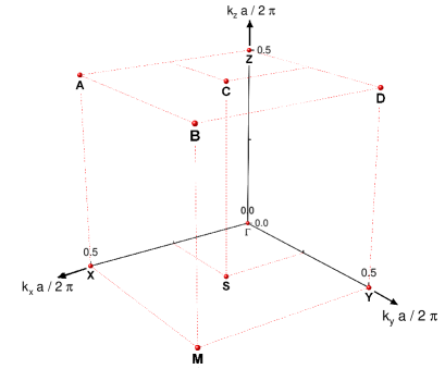
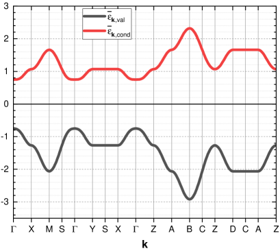
Figure 1: (top) High-symmetry points in the first Brillouin zone. (bottom) Equilibrium energy bands, $\bar{\varepsilon}_{\mathbf{k},\mathrm{val}}$ and $\bar{\varepsilon}_{\mathbf{k},\mathrm{cond}}$, along the main path.

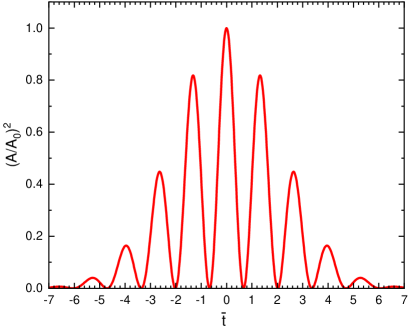
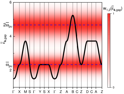
Figure 2: (top) The square of the pumping vector potential as a function of time. (bottom) The energy gaps, $\bar{\varepsilon}_{\mathbf{k},\mathrm{gap}}$, along the main path. The colored map shows $w_{l=1,2}\left(\bar{\varepsilon}_{\mathbf{k},\mathrm{gap}}\right)$ for one- and two-photon resonances.

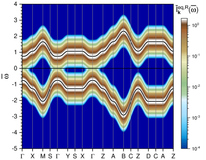
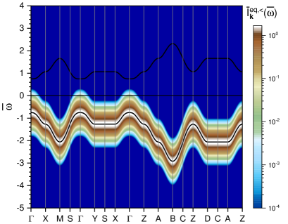
Figure 3: TR-ARPES signals at equilibrium, (top) $\bar{I}_{\mathbf{k}}^{\mathrm{eq},R}\left(\bar{\omega}\right)$ and (bottom) $\bar{I}_{\mathbf{k}}^{\mathrm{eq},<}\left(\bar{\omega}\right)$. The solid black curves show the equilibrium energy bands.

III A two-band lattice system: a noteworthy application

Very recently, we have proved the capabilities of DPOA in investigating real materials by exploiting it to analyze the actual photo-injection mechanisms in germanium within an ultrafast (attosecond) pump-probe setup [30]. To discuss the variety of possible physical phenomena without being limited by the characteristics of a single particular real material, here we choose to study a cubic lattice system, of lattice constant $a$, with two bands corresponding to the main valence and conduction bands in a semiconductor. We consider two states (MLWFs) with the onsite energies $\tilde{T}_{\mathbf{R}=\boldsymbol{0},1,1}=-1.65\Delta$ and $\tilde{T}_{\mathbf{R}=\boldsymbol{0},2,2}=1.35\Delta$, respectively, diagonal first-neighbor hoppings $\tilde{T}_{\mathbf{R}=\boldsymbol{\delta},1,1}=0.2\Delta$ and $\tilde{T}_{\mathbf{R}=\boldsymbol{\delta},2,2}=-0.15\Delta$, and off-diagonal first-neighbor hoppings $\tilde{T}_{\mathbf{R}=\boldsymbol{\delta},1,2}=\tilde{T}_{\mathbf{R}=\boldsymbol{\delta},2,1}=-0.1\Delta$, where $\tilde{T}_{\boldsymbol{R},\nu,\nu^{\prime}}$ is the hopping matrix between two sites at distance $\boldsymbol{R}$ and states $\nu$ and $\nu^{\prime}$, respectively, $\boldsymbol{\delta}\in\left\{a\left(\pm 1,0,0\right),a\left(0,\pm 1,0\right),a\left(0,0,\pm 1\right)\right\}$ and $\Delta$ is the unit of energy that can be adjusted to obtain the desired band gap energy at $\Gamma=\left(0,0,0\right)$. With our parameters, the band gap at $\Gamma$ is $1.5\Delta$, so that in order to have a gap of $0.75\,\mathrm{eV}$ for instance, one should set $\Delta=0.5\,\mathrm{eV}$. For the cases that we analyze with a finite dipole, we consider an on-site (local) and off-diagonal dipole moment: $\tilde{\mathbf{D}}_{\mathbf{R}=\boldsymbol{0},1,2}=\tilde{\mathbf{D}}_{\mathbf{R}=\boldsymbol{0},2,1}^{*}=\mathrm{i}0.05a\hat{\mathbf{j}}$, which will lead only to a $0$-th term in its Peierls expansion.

In Fig. 1, top panel, we show the high-symmetry points of the first Brillouin zone, while in the bottom panel we show the equilibrium energy bands, $\bar{\varepsilon}_{\mathbf{k},\mathrm{val}}=\varepsilon_{\mathbf{k},1}/\Delta$ and $\bar{\varepsilon}_{\mathbf{k},\mathrm{cond}}=\varepsilon_{\mathbf{k},2}/\Delta$, for a path which connects these high-symmetry points (the main path hereafter). All energies denoted with a bar on top are divided by $\Delta$ and hence dimensionless. Having $\Delta$ as the unit of energy, the unit of time is simply chosen to be $\hbar/\Delta$, which results in the dimensionless time $\bar{t}=t\Delta/\hbar$ for each time $t$.

We apply a pump pulse in the form $\boldsymbol{A}\left(\bar{t}\right)=A\left(\bar{t}\right)\hat{\mathbf{j}}$ where $A\left(\bar{t}\right)$ is a wave packet given by

$$A\left(\bar{t}\right)=\frac{2\pi\hbar}{a\mathrm{e}}\bar{A}_{0}e^{-\left(4\ln 2\right)\bar{t}^{2}/\bar{\tau}_{\mathrm{pu}}^{2}}\cos\left(\bar{\omega}_{\mathrm{pu}}\bar{t}\right),$$ (54)

in which the center of the pump pulse is taken as the origin of time axis. The dimensionless frequency of the pump pulse is chosen to be $\bar{\omega}_{\mathrm{pu}}=\omega_{\mathrm{pu}}\hbar/\Delta=2.33$ and, unless otherwise explicitly stated, the FWHM is chosen to be $\bar{\tau}_{\mathrm{pu}}=7$ and the dimensionless pump-pulse amplitude $\bar{A}_{0}=0.2$.

The square of the pumping vector potential as a function of time is plotted in Fig. 2, top panel. Fig. 2 bottom panel shows the energy gaps, $\bar{\varepsilon}_{\mathbf{k},\mathrm{gap}}=\bar{\varepsilon}_{\mathbf{k},\mathrm{cond}}-\bar{\varepsilon}_{\mathbf{k},\mathrm{val}}$, at the k points along the main path, while the colored map shows $w_{l=1,2}\left(\bar{\varepsilon}_{\mathbf{k},\mathrm{gap}}\right)$, which indicates the strength of $l$-photon resonance for each energy gap.

For TR-ARPES signal, we apply a probe pulse with FWHM of $\bar{\tau}_{\mathrm{pr}}=\bar{\tau}_{\mathrm{pu}}=7$, unless otherwise explicitly stated. We study the dimensionless signals that are obtained as $\bar{I}_{\mathbf{k}}^{R,<}=\nicefrac{{\Delta}}{{\hbar}}I_{\mathbf{k}}^{R,<}$. In Fig. 3, we show $\bar{I}_{\mathbf{k}}^{\mathrm{eq},R}\left(\bar{\omega}\right)$ and $\bar{I}_{\mathbf{k}}^{\mathrm{eq},<}\left(\bar{\omega}\right)$ at equilibrium, that is when no pump pulse is applied to the system. The finite width of the probe pulse results in a broadening of the levels, which is intrinsic to quantum mechanics and unavoidable. Increasing the FWHM of the probe pulse, one can decrease this broadening, but we are not interested in probe pulses much wider than the pump-pulse envelope. The retarded signal, $\bar{I}_{\mathbf{k}}^{\mathrm{eq},R}\left(\bar{\omega}\right)$, is peaked around both valence and conduction band energies and shows the spectrum of the system, while the lesser signal, $\bar{I}_{\mathbf{k}}^{\mathrm{eq},<}\left(\bar{\omega}\right)$, shows the occupied valence-band levels only, which is the signal measured in experiments.

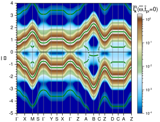
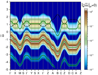
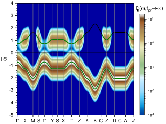
Figure 4: TR-ARPES signals for the case of local dipole coupling. (left) $\bar{I}_{\mathbf{k}}^{R}\left(\bar{\omega},\bar{t}_{\mathrm{pr}}=0\right)$ and (middle) $\bar{I}_{\mathbf{k}}^{<}\left(\bar{\omega},\bar{t}_{\mathrm{pr}}=0\right)$: the center of the probe pulse coincides with the center of the pump pulse. (right) $\bar{I}_{\mathbf{k}}^{<}\left(\bar{\omega},\bar{t}_{\mathrm{pr}}\rightarrow\infty\right)$: after the pump pulse is turned off. The black solid curves mark the equilibrium band energies. The green dots indicate the local maxima in energy of the signals for each $\mathbf{k}$: the (out-of-equilibrium) bands of TR-ARPES.

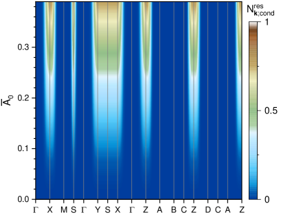
Figure 5: Local dipole coupling case: (top) Residual excited electronic population along the main path as a function of the pump-pulse amplitude. (bottom) Residual excited electronic population at S as a function of the amplitude and of the FWHM of the pump pulse.

III.1 Local dipole coupling (no Peierls substitution)

As first case, we consider a Hamiltonian in which the coupling to the pumping field comes only through a local dipole moment, i.e., we neglect the Peierls substitution in the hopping term and in the dipole one (in Eq. 18 we set $\mathbf{k}+\frac{e}{\hbar}\boldsymbol{A}\left(t\right)\rightarrow\mathbf{k}$), to focus only on the effects of such a coupling on the system and analyze them in detail. This case is relevant to systems such as quantum dots and molecules, and low-dimensional systems with transverse pumps.

In Fig. 4, we show the maps of TR-ARPES signals along the main path. The left panel shows the retarded signal, $\bar{I}_{\mathbf{k}}^{R}\left(\bar{\omega},\bar{t}_{\mathrm{pr}}=0\right)$, for the case where the center of the probe pulse coincides with the center of the pump pulse. The valence and conduction bands are more broad than at equilibrium (Fig. 3) because the electrons get excited to the conduction band and cannot be assigned to a specific band anymore, inducing a quantum-mechanical uncertainty in the energy of the bands themselves.

The photon-side-bands (PSBs) emerge at energies that differ from the main-band energies of integer multiples of the (dressed) pump-pulse photon energy. Some PSBs overlap in energy with the conduction and the valence bands and, therefore, are not distinguishable in the map of the retarded signal.

On top of the maps, we reported both the equilibrium band energies (black solid curves) and the local maxima in energy of the signals at each $\mathbf{k}$ (green dots), that indicate the (out-of-equilibrium) bands of TR-ARPES. As the retarded signal shows, the equilibrium valence and conduction bands coincide with TR-ARPES ones: a local dipole, for realistic intensities, has negligible effects on the TR-ARPES bands of the system.

Since in equilibrium only the valence band is occupied, the lesser signal, $\bar{I}_{\mathbf{k}}^{<}\left(\bar{\omega},\bar{t}_{\mathrm{pr}}=0\right)$, which is reported in the middle panel of Fig. 4, shows only the valence band and its corresponding PSBs. Wherever (in $\mathbf{k}$ space) we have a one-photon resonance, the related resonant one-photon PSB is definitely stronger than other PSBs as it coincides with the conduction band in this case. The two-photon PSBs are some orders of magnitude weaker than the one-photon ones and, in the scale we have chosen for the maps, it is not possible to see them.

If we probe the system after the pump pulse is turned off, i.e., by setting a large $\bar{t}_{\mathrm{pr}}\rightarrow+\infty$, but still much shorter than the time scale of other decoherence and recombination processes like spontaneous emission or electron-phonon interaction, the spectrum of the system goes back to equilibrium, so that we have $\bar{I}_{\mathbf{k}}^{R}\left(\bar{\omega},\bar{t}_{\mathrm{pr}}\rightarrow+\infty\right)=\bar{I}_{\mathbf{k}}^{R}\left(\bar{\omega},\bar{t}_{\mathrm{pr}}\rightarrow-\infty\right)$, which is already shown in Fig. 3 and we do not repeat here.

In Fig. 4, right panel, we report $\bar{I}_{\mathbf{k}}^{<}\left(\bar{\omega},\bar{t}_{\mathrm{pr}}\rightarrow+\infty\right)$: contrarily to what happens for the retarded signal, the lesser signal shows residual effects at the k points for which the pump-pulse frequency is in one-photon resonance with the equilibrium gap energy. The more-than-one-photon PSBs do not show any residual signal even though at $\bar{t}_{\mathrm{pr}}=0$ they are non-vanishing. This is because we have only a local dipole in the interaction Hamiltonian and such a term have no $\cos\left(l\bar{\omega}_{\mathrm{pu}}\bar{t}\right)$ term for $l>1$, hence no more-than-one-photon Rabi-like resonances. According to our experience, this can be overcome having more than two bands in the system (not shown).

In Fig. 5, top panel, we plot the residual excited electronic population in the conduction band, $N_{\mathbf{k},\mathrm{cond}}^{\mathrm{res}}$, for the k points along the main path as a function of the pump-pulse amplitude. Rabi-like oscillations induce residual excited populations at the k points for which a one-photon resonance condition is realized. The finite width of the pump pulse broadens the resonant energies so that, in addition to the exact resonances, also the k points in the proximity of resonant ones have some residual excited population (compare with Fig. 2).

In Fig. 5, bottom panel, we plot the residual excited population in the conduction band at S as a function of the amplitude and of the FWHM of the pump pulse. Being (i) the Rabi frequency, $\Omega_{R}$, proportional to the pump-pulse amplitude and (ii) the overall oscillation time roughly proportional to the FWHM of the pump pulse, the residual excited population is almost constant wherever $\bar{A}_{0}\bar{\tau}_{\mathrm{pu}}$ is constant, that yields the hyperbolic shape of the color contours in the figure. For the very same reason, on both cuts at fixed $\bar{A}_{0}$ and at fixed $\bar{\tau}_{\mathrm{pu}}$, one clearly sees the signature of the Rabi-like oscillations. For instance, at fixed $\bar{A}_{0}$, that is at fixed $\Omega_{R}$, the end tail (in time) of the pump-pulse envelope determines the residual excited population and on changing $\bar{\tau}_{\mathrm{pu}}$ one can scan the Rabi-like oscillating behavior of the population (roughly $N_{\mathbf{k};\mathrm{cond}}^{\mathrm{res}}\propto\sin^{2}\left(\Omega_{R}\tau_{\mathrm{pu}}\right)$). It is worth reminding that, for smaller pump-pulse amplitudes, which are those experimentally more relevant, one can approximate $\sin\left(\Omega_{R}\tau_{\mathrm{pu}}\right)\simeq\Omega_{R}\tau_{\mathrm{pu}}$, which results in $N_{\mathbf{k};\mathrm{cond}}^{\mathrm{res}}\propto\bar{A}_{0}^{2}\bar{\tau}_{\mathrm{pu}}^{2}$.

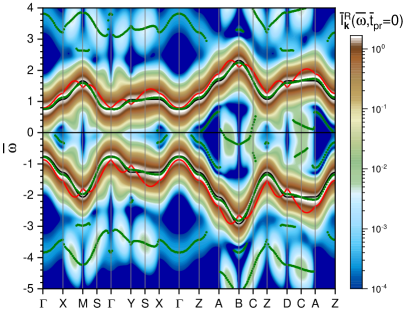
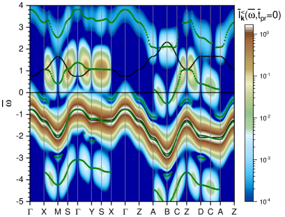
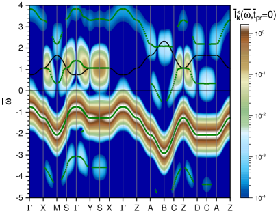
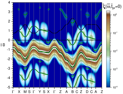
Figure 6: TR-ARPES signals along the main path for Peierls substitution in the hopping term and no dipole, with the center of probe pulse coinciding with the one of pump pulse ($\bar{t}_{\mathrm{pr}}=0$ ). (top-left) $\bar{I}_{\mathbf{k}}^{R}\left(\bar{\omega},\bar{t}_{\mathrm{pr}}=0\right)$ and (top-right) $\bar{I}_{\mathbf{k}}^{<}\left(\bar{\omega},\bar{t}_{\mathrm{pr}}=0\right)$ for the full dynamics, (bottom-left) $\bar{I}_{\mathbf{k}}^{R}\left(\bar{\omega},\bar{t}_{\mathrm{pr}}=0\right)$ for the dynamics with inter-band-only transitions, and (bottom-right) $\bar{I}_{\mathbf{k}}^{<}\left(\bar{\omega},\bar{t}_{\mathrm{pr}}=0\right)$ for the dynamics with intra-band-only transitions. The black-solid curves show the equilibrium band energies while the green dots indicate the local maximum of the signals for each k point, which are the (out-of-equilibrium) bands of TR-ARPES. The red-solid curves show the instantaneous eigenenergies at time zero.

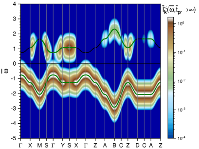
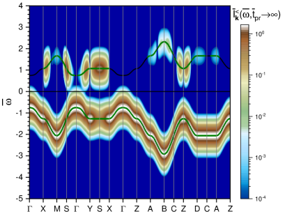
Figure 7: Residual lesser TR-ARPES signal along the main path for only Peierls substitution with zero dipole, considering (top) full dynamics, and (bottom) inter-band-only dynamics. The black-solid curves show the equilibrium band energies while the green dots show the local maximum of the signals for a fixed k point.

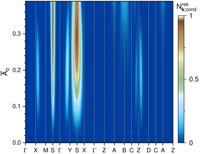
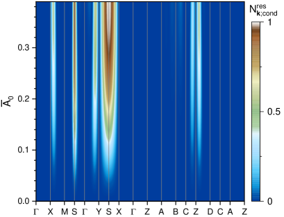
Figure 8: Residual excitations along the main path as a function of the pump-pulse amplitude for the case of Peierls substitution in the hopping term and zero dipole. (top) The full dynamics. (bottom) The dynamics considering inter-band transitions only.

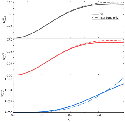
Figure 9: Residual excited population per unit cell as a function of the pump-pulse amplitude for a $8\times 8\times 8$ k grid over the first Brillouin zone, considering Peierls substitution in the hopping term and no dipole. (top) all (any-photon) resonant contributions, (middle) only one-photon resonant contributions and (bottom) only two-photon resonant contributions. In all panels, we report the two cases of the full original Hamiltonian (solid) and inter-band-only Hamiltonians (dots).

III.2 Peierls substitution in hopping (no dipole)

In this case, we consider an interaction with the pump pulse via the Peierls substitution in the hopping term and set the dipole to zero. This is very relevant as the dipole term is often negligible in many realistic cases. Moreover, neglecting the dipole we can focus on the effects of band symmetries on TR-ARPES signal and electronic excitations and analyze them in detail.

In Fig. 6 top-left (top-right), we show the map of $\bar{I}_{\mathbf{k}}^{R}\left(\bar{\omega},\bar{t}_{\mathrm{pr}}=0\right)$ ($\bar{I}_{\mathbf{k}}^{<}\left(\bar{\omega},\bar{t}_{\mathrm{pr}}=0\right)$). The higher local maxima of the TR-ARPES signal, that one can consider the main TR-ARPES bands, are slightly shifted with respect to the equilibrium valence and conduction bands and show almost no correspondence to the instantaneous eigenenergies at time zero. This is expected since TR-ARPES measures the system over a time period and not at a specific instant of time. We will shed more light on this issue later on (Fig. 14 and related discussion). For the retarded signal, which shows the full TR-ARPES spectrum of the system, we can see both valence and conduction bands and all of their sidebands. Because of the finite broadening of the bands, they overlap and distinguishing them in the case of retarded signal can be very difficult. Obviously, in the lesser signal, we see only the valence band and its sidebands.

The one-photon PSBs originate from the velocity term in the Peierls expansion, which is proportional to $\sin\left(ak_{y}\right)$ and, therefore, identically vanishes on the planes $\boldsymbol{\Gamma}$-X-A-Z and Y-M-B-D, yielding no one-photon PSB there. Instead, on S, C, middle points of the lines X-M, A-B, Z-D and $\boldsymbol{\Gamma}$-Y, the second order (inverse-mass) term – as well as all other even terms – of the Peierls expansion vanishes as it is proportional to $\cos\left(ak_{y}\right)$. Recall that the polarization of the pump-pulse has been chosen along the $y$ direction.

However, even though at some of these points the two-photon PSBs are very weak, at some others (such as S), where we have a strong one-photon PSB, the two-photon PSB is also strong, which shows that the second order signal is assisted by multiple actions of the first order terms of the Hamiltonian. At the k points where the band gap is at either one- or two-photon resonance with the pump pulse, the corresponding PSB is much stronger than non resonant ones, provided that it is not zero by symmetry.

At the k points where the inverse-mass vanishes, we have practically no shift of the TR-ARPES bands with respect to the equilibrium ones. The shift in the bands is mainly due to the non-oscillating components that appear in the even order terms of Peierls expansion ($\sum_{m=1}^{\infty}\Theta_{0,m}\left(t\right)$ in Eq. 28), which identically vanish when the inverse-mass vanishes by symmetry. Moreover, the higher order effects of the same term results in some weak side-bands near the main bands as it is more clear in the map of $\bar{I}_{\mathbf{k}}^{<}\left(\bar{\omega},\bar{t}_{\mathrm{pr}}=0\right)$ (top-right panel). It is worth noting that if we had an infinitely oscillating pump pulse without an envelope (that is, a pump-pulse FWHM extremely longer than the probe-pulse FWHM), there would have been no higher order effects and the non-oscillating components would have just resulted in rigid shifts of the bands. Therefore, we dub these new side-bands as envelope-Peierls side-bands (EPSBs): they are due to both the envelope and the even terms of Peierls expansion.

In Fig. 6, bottom-left (bottom-right) panel, we show the map of $\bar{I}_{\mathbf{k}}^{<}\left(\bar{\omega},\bar{t}_{\mathrm{pr}}=0\right)$ for the dynamics with inter-band-only (intra-band-only) transitions. Interestingly, the main TR-ARPES bands are practically on top of the equilibrium ones in the case of inter-band-only dynamics. On the other hand, for the case of intra-band-only dynamics, we see the same shift as for the full dynamics. This is consistent with the inter-band transitions governing the electronic transitions between the bands and not altering the bands noticeably, while the intra-band transitions change the band energies dynamically. As we already mentioned above, the shift in the main bands have the same origin as the EPSBs and since we do not have band shifts for inter-band-only transitions, the EPSBs disappear as well.

PSBs have different behaviors depending on being one-photon or two-photon, and in resonance or off resonance. The resonant one-photon PSBs are much stronger in the inter-band-only case (bottom-left panel) than in the intra-band-only case (bottom-right panel), because in order to differentiate between in resonance and off resonance, one needs the inter-band transitions. On the contrary, the off-resonant one-photon PSBs are stronger in the intra-band-only case than in the inter-band-only one, which shows that for the system parameters that we have chosen, out of resonance, the inter-band transitions have very negligible effects on the system, while intra-band transitions obviously still induce one-photon PSBs. In fact, in the intra-band-only case, our system is equivalent to a single-band (the valence band) Floquet one as the conduction band is obviously empty and not coupled to the valence band. However, in our system, in the inter-band-only case (bottom-left panel), two-photon off-resonance PSBs can be noticeable in comparison to the case of full dynamics (top-right panel).

The resonant one-photon (two-photon) PSBs are stronger (weaker) in the case of full dynamics than in the case of the inter-band-only dynamics. This can be understood by noticing that removing intra-band transitions pins down the electrons at one-photon resonant k points and helps them to get more and more excited, while lack of the inter-play between first-order inter- and intra-band transitions reduces the two-photon resonant PSBs. In fact, considering a Hamiltonian with even terms only in the Peierls expansion (no first – velocity – and higher-order odd terms) and removing the intra-band transitions, one obtains stronger PSBs at the two-photon resonances (not shown).

Another important property to be studied is the residual signal of TR-ARPES. As we already mentioned, after the action of pump pulse, the spectrum which is given by the retarded signal is exactly the one of equilibrium (Fig. 3), while the lesser signal is different. As shown in Fig. 7 top panel, where we plot $\bar{I}_{\mathbf{k}}^{<}\left(\bar{\omega},\bar{t}_{\mathrm{pr}}\rightarrow\infty\right)$, at the one- or two-photon resonant k points we have the corresponding residual signals at PSBs, unless the PSB is prohibited by symmetry. For instance, this condition realizes for one-photon PSBs at X, Y, and Z, where we have exact one-photon resonances, and for two-photon PSBs at the middle of A-B and at C, where we have non-exact two-photon resonances.

Fig. 7 bottom panel, shows the residual lesser signal for the dynamics given by inter-band-only transitions. The one-photon (two-photon) residual PSBs are stronger (weaker) for the inter-band-only dynamics than for the full one according to the very same reasoning reported above. It is noteworthy that even though the intra-band-only transitions induce PSBs within the pump-pulse envelope (see Fig. 6, bottom-right panel), they yield no residual in the TR-ARPES signal, which return to equilibrium after the pump pulse is turned off (Fig. 3).

In Fig.␣8, top panel, we plot the residual excited populations along the main path as a function of the pump-pulse amplitude. One- and two-photon resonances have residual excited populations that show Rabi-like oscillations with respect to changing the pump-pulse amplitude. Moreover, unlike in the former case (only local dipole), k points with the same gap energies (for example those along the path Y-S-X) have different behaviors as their velocities and inverse-masses are different, which yields different couplings to the pumping field. In particular, at the $\mathbf{k}$ points where we have one-/two-photon resonances, but the velocity/inverse mass vanishes (see the related discussion above on the TR-ARPES signal regarding the relevant regions of first Brillouin zone), there are no residual excitations. However, the points at their immediate proximities with non-exact resonant gaps, but non-zero velocities/inverse masses, host some residual excited populations.

In Fig.␣8, bottom panel, we see that for the case of a dynamics with just the inter-band transitions, the residual excited population coming from one-photon resonances gets larger (on the contrary, if one keeps only the intra-band transitions there would be no excitations at all). In this case, one-photon resonances get stronger because we have removed the intra-band transitions that drive them transiently out of resonance and leads to a smaller residual excited population. However, there are some weak one-photon resonances that benefit from intra-band transitions since they are far from the exact resonant points and by the intra-band transitions they can get transiently closer to resonance. The net effect for them is to gain some residual excited population so that the related resonant region in $\mathbf{k}$-space appears wider. An example can be the proximities of the S point on the path M-S-$\boldsymbol{\Gamma}$. On the other hand, for the two-photon resonances this will result in smaller residual excited populations. The two-photon resonances are assisted by the inter-play between the inter-band and intra-band contributions of the first term of the Peierls expansion, which is removed by removing the intra-band transitions altogether (similar to TR-ARPES signal). In fact, also in this case, considering a Hamiltonian with even terms only in the Peierls expansion and removing the intra-band transitions, one obtains larger and sharper in k-space residual excitations at the two-photon resonances (not shown).

In Fig. 9, top panel, we plot the total residual excited population per unit cell, Eq. 37, as a function of the pump-pulse amplitude. We have considered a $8\times 8\times 8$ k-grid to sample the first Brillouin zone, even though we checked the robustness of the results with respect to the size of the grid by using also $16\times 16\times 16$ and $32\times 32\times 32$ k-grids for a larger step in the pump-pulse amplitude (not shown). We compare the two cases: the full Hamiltonian and the one with inter-band transitions only. For all values of the pump-pulse amplitude, the total residual excited population with only inter-band transitions is larger. The middle (bottom) panel of Fig. 9, shows the contribution from one-photon (two-photon) resonances, i.e., Eq. 36 with $l=1$ ($l=2$). In our system, the largest contribution comes from the one-photon resonances (middle panel). Computing the relative multi-photon resonance strengths (see Eq. 31) in our grid, we find out that the relative strength of one-photon ($l=1$) resonances is 64%, while for two-photon ($l=2$) resonances is 36% ($W_{l}/\left(W_{1}+W_{2}\right)$, see Eq. 31). Clearly, these numbers do not take into account the actual strength of the system-pump couplings at these resonant $\mathbf{k}$ points and that the second order transitions are generally weaker than the first order ones.

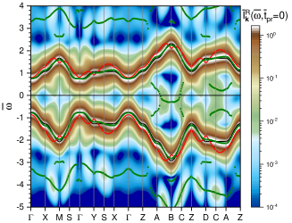
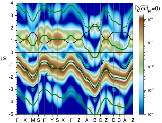
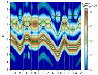
Figure 10: The TR-ARPES signal considering both Peierls substitution and local dipole in the Hamiltonian, with the probe and pump pulses having the same center, i.e., $\bar{t}_{\mathrm{pr}}=0$. (right) the retarded signal, (middle) the lesser signal, and (left) the lesser signal for inter-band-only transitions. The black-solid curves show the equilibrium band energies while the green dots show the local maxima of the signals for a fixed k point. The red-solid curves show the instantaneous eigenenergies at time zero.

As we already explained above in detail, for the one-photon resonances (middle panel), the removal of intra-band transitions increases the residual excited populations, while for the two-photon resonances (bottom panel), the residual excited populations get reduced by removal of the intra-band transitions. In the latter case, increasing the pump-pulse amplitude to high values, the behavior changes and the results of inter-band-only Hamiltonian overcome the full Hamiltonian ones. This can be understood by noting that, upon removing intra-band transitions, the Rabi-like oscillations become in average slower over all of the two-photon resonant k points and of the sin-like shape we see only the monotonously increasing behavior that eventually manages to overcome the usual bending-over sin-like behavior in the case of the full Hamiltonian. This results in a higher residual excitation for very high amplitudes of the pump pulse in the case of inter-band-only and two-photon resonances. It is noteworthy that such very high pump-pulse intensities are not affordable in realistic setups as they would damage the sample.

III.3 Both Peierls substitution and local dipole

In this section, we consider both local dipole and Peierls substitution with the related Hamiltonian parameter values given in the former two cases. In this case, even though some of the effects can be explained by simply considering the mere addition of the effects yielded by the individual coupling terms, we clearly see that the interplay between the two interaction terms is very important.

The retarded TR-ARPES signal along the main path at $\bar{t}_{\mathrm{pr}}=0$ is shown in Fig. 10, left panel, while the lesser TR-ARPES signal is shown in the middle panel. The local dipole strengthens both one-photon and two-photon PSBs. In this case, the k points with zero velocity do have one-photon PSBs, because of the local dipole which does not follow the symmetry of the bands. The TR-ARPES bands are definitely closer to the equilibrium bands rather than to the instantaneous eigenenergies. The presence of both coupling terms augments the broadening of the signals as it increases the excited population overall and, in particular, at the main resonant k point, S.

Looking at the inter-band-only lesser TR-ARPES signal, which is shown in the right panel, we see similar behaviors to the case of zero dipole, except for one main difference: the reduction in the two-photon resonant signal is much stronger. As a matter of fact, the inter-play between inter-band and intra-band first-order terms assists the second-order two-photon resonance and is strengthened by the cooperation of Peierls substitution and dipole. It is worth noticing that we considered the local dipole to be just of inter-band form, therefore, the intra-band-only results are exactly the same as the case of zero dipole, which were presented in Fig. 6, bottom-right panel.

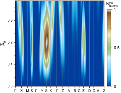
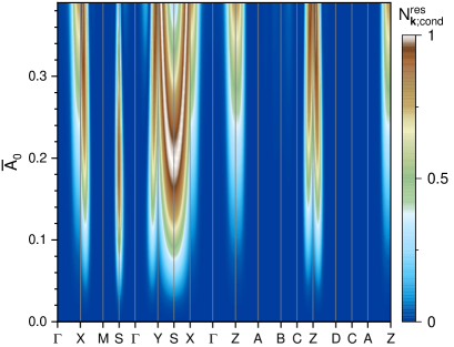
Figure 11: Residual excitation along the main path as a function of the pump-pulse amplitude for the case of both Peierls substitution and local dipole. (top) Full dynamics, (bottom) dynamics with inter-band transitions only.

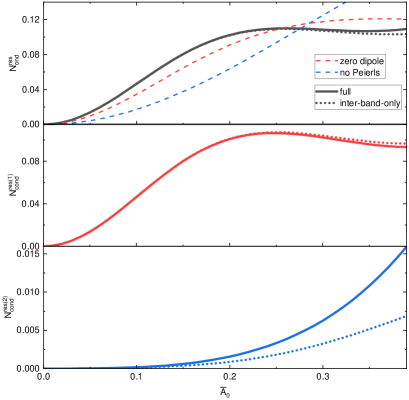
Figure 12: Residual excitation per unit cell as a function of the pump-pulse amplitude for a $8\times 8\times 8$ k grid over the first Brillouin zone, considering both Peierls substitution and local dipole. (top) All (any-photon) resonant contributions, (middle) one-photon and (bottom) two-photon resonance contributions. In all panels, we report the two cases of the full original Hamiltonian (solid) and inter-band-only Hamiltonians (dots). In the top panel, the results of zero dipole (red dashed) and Peierls-substitution-only (blue dashed) cases are also reported.

In Fig. 11 top panel, we plot the residual excited population along the main path vs the pump-pulse amplitude. The first important change with respect to the zero dipole case is that the one-photon resonant k points with zero velocity (X, Y, and Z) do have residual excited population now: the symmetry protection is lost in the presence of the dipole term (as discussed for the TR-ARPES signal). Moreover, having both local dipole and Peierls substitution increases the Rabi frequency on the line X-S-Y which yields the residual excited population at S to have a maximum at around the pump-pulse peak amplitude of $\bar{A}_{0}\simeq 0.19$, showing more clearly the Rabi-like behavior.

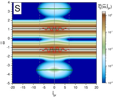
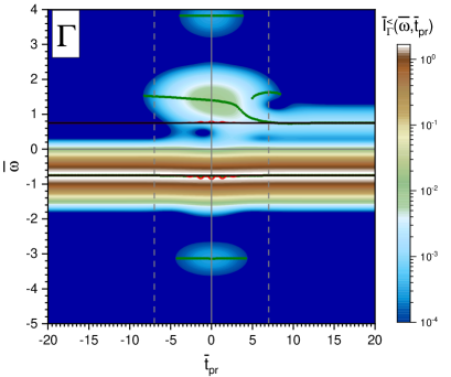
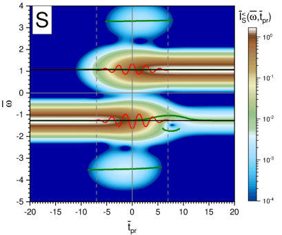
Figure 13: (top) The retarded and (bottom) the lesser TR-ARPES signals vs the center of probe-pulse envelope, $\bar{t}_{\mathrm{pr}}$, for the high-symmetry points (left) $\boldsymbol{\Gamma}$ and (right) S. The vertical dashed gray lines determine $\pm\bar{\tau}_{\mathrm{pu}}$. The black-solid lines show the equilibrium band energies while the green dots show the local maximum of the signals for a fixed k point. The red-solid curves show the instantaneous eigenenergies as functions of $\bar{t}_{\mathrm{pr}}$.

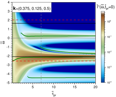
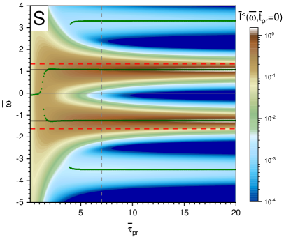
Figure 14: The lesser TR-ARPES signals vs the FWHM of probe-pulse envelope, $\bar{\tau}_{\mathrm{pr}}$, while the center of probe pulse is kept at $\bar{t}_{\mathrm{pr}}=0$, for (top) the k point $\mathbf{k}=\left(0.375,0.125,0.5\right)$ and (bottom) the high-symmetry point S. The vertical dashed gray lines determine $\bar{\tau}_{\mathrm{pu}}$. The black-solid lines show the equilibrium band energies while the green dots show the local maximum of the signals for a fixed k point. The red-solid lines show the instantaneous eigenenergies at time zero.

In Fig. 11 bottom panel, we plot the residual excited population keeping only inter-band transitions in the dynamics. Removing the intra-band transitions, noticeably increases the residual excited population at the resonance points near X and Y, so that they can also reach the maximum of full population inversion. Moreover, for the two-photon resonant k points, the difference between full and inter-band-only dynamics is much larger than in the case of zero dipole (as discussed for TR-ARPES signal).

After investigating the residual excitation on the main path, we discuss the excitation per unit cell, which is obtained using a $8\times 8\times 8$ k grid to sample the first Brillouin zone and plotted in the top panel of Fig. 12. Comparison with the two former cases of considering no Peierls substitution and having zero dipole (both shown in the same panel), we see the maximum occurs at a smaller pump-pulse amplitude, as the local dipole adds up to the Peierls substitution which increases the Rabi frequencies at one-photon resonant k points. Another relevant feature is related to only-inter-band transitions in the dynamics that seem to reduce the residual excited population, which is apparently in contradiction with the result of Fig. 9. However, the behavior of one-photon and two-photon resonance contributions, as plotted in the middle and bottom panels of Fig. 12, reveals that similar to the case of zero dipole, the inter-band-only dynamics gives more (less) residual excited population for the one-photon (two-photon) resonance contributions, but the difference between the inter-band-only and full dynamics of the two-photon resonances are much larger in this case, as we explained in the discussion of Fig. 10.

III.4 More on the characteristics of the TR-ARPES signal

In this section, we get more insights about the behavior of the system out of equilibrium by changing the probe-pulse parameters. For the coupling Hamiltonian, we consider both local dipole and Peierls substitution, but the general conclusions we will draw are independent of this choice.

First, we study how the TR-ARPES signal changes on varying the center of probe pulse, $\bar{t}_{\mathrm{pr}}$, from before (equilibrium) to after (possible residual excitations) the pump-pulse envelope. The retarded and lesser TR-ARPES signals for two high-symmetry k points, $\boldsymbol{\Gamma}$ and S, are reported in Fig. 13, top panels. For both k points, the PSBs are detected as soon as the probe-pulse center enters the pump-pulse envelope, that is when the instantaneous eigenenergies become different from the equilibrium band energies.

At equilibrium, as expected, the lesser signal (bottom panels) shows that the electrons reside in the valence band, while they get excited into the conduction band during the pump-pulse application. At S, which is exactly one-photon resonant, we register an almost complete population inversion as the electron excitation process is really very efficient.

After the pump pulse is turned off, the residual signal at $\boldsymbol{\Gamma}$ is very weak ($\boldsymbol{\Gamma}$ is not in resonance), while at S we have a very strong residual signal because of the resonance condition. Having both local dipole and Peierls substitution, yields slightly more residual signal compared to the cases of removing one of the two coupling terms.

Moreover, at S we have the splitting of the valence band. Such a splitting is not visible at time $\bar{t}_{\mathrm{pr}}=0$, because the two wide split bands overlap with each other. Increasing either the local dipole or the pump-pulse amplitude one can see the splitting even at time $\bar{t}_{\mathrm{pr}}=0$ (not shown). The splitting can be seen only in the lesser signal, which is the actual signal measured in the experiments, and not in the retarded one, and, accordingly, is due to the holes photo-injected in the system by resonant pumping of the valence electrons into the conduction band (photo doping).

So far, the FWHM of the probe pulse was kept constant and equal to the one of the pump pulse, $\bar{\tau}_{\mathrm{pu}}=\bar{\tau}_{\mathrm{pr}}=7$. Now, we study the effect of varying $\bar{\tau}_{\mathrm{pu}}$ while keeping $\bar{t}_{\mathrm{pr}}=0$. In Fig. 14, the lesser signal is reported at an off-resonant k point $\left(0.375,0.125,0.5\right)$ (top panel) and at the resonant k point S (bottom panel). The former point is chosen in order to have an energy difference between the instantaneous eigenenergies at time zero and the equilibrium-band energies quite noticeable to better illustrate the phenomenology we are going to discuss.

First, we analyze the behavior at the off-resonant k point (top panel). For very narrow probes, that is small $\bar{\tau}_{\mathrm{pr}}$ with respect to $\bar{\tau}_{\mathrm{pu}}$, by decreasing $\bar{\tau}_{\mathrm{pr}}$, the signal gets wider and its peaks tend to the instantaneous eigenenergies. This indicates that the system is practically in the lower eigenstate, which is predominantly valence-band-like as there is no excitation to the higher eigenstate. At any rate, the peaks will never exactly coincide with the instantaneous eigenenergies (even though they are very close to them) as the process is not adiabatic. We expect this also in real semiconductors and insulators as there the off-diagonal terms of the coupling Hamiltonian are usually much smaller than the energy gaps determined by the total Hamiltonian.

Instead, increasing the width of the probe-pulse envelope, $\bar{\tau}_{\mathrm{pr}}$, corresponds to measuring the system over a finite time interval and, practically, to performing a time average over such an interval. This averaging process results in the emergence of side-bands while the main peaks tend to the equilibrium bands. The shifts of the bands are due to the high non-linearity of the processes and to the non-zero average of the oscillating pump pulse. The PSBs remain at almost fixed energies after they emerge because they are related to the oscillating component of the pumping field and, if the probe pulse is wide enough to see the oscillations, it does not matter how much wider it becomes. On the other hand, EPSBs change their energies by changing the width of the probe-pulse envelope, because they are driven by the non-oscillating component of the pumping field.

By increasing the width of the probe pulse to very high values, the resolution in energy increases and the peaks become very sharp. However, having such a large probe-pulse FWHM corresponds to (i) reduce more and more the time resolution of the measurement and (ii) include more and more equilibrium behavior (before pump-pulse envelope) and residual effects (after pump-pulse envelope) into the measurement. Therefore, we cannot obtain enough information about the real-time out-of-equilibrium dynamics of the system. On the other hand, on decreasing the width of the probe pulse, the signals become very wide in energy. This requires more and more experimental resolution in energy to determine the position of the peaks and understand the physics. Consequently, one needs to choose some intermediate value in order to cope with the unavoidable intrinsic time-energy uncertainty relationship of the underlying quantum mechanical system.

The situation at resonance is quite different. As it is shown in the bottom panel of Fig. 14, even for the smallest values of $\bar{\tau}_{\mathrm{pu}}$, the peak of lesser TR-ARPES signal does not coincide with the lower eigenenergy as the resonant dynamics forces the electrons to evolve in a superposition of valence and conduction band states. The superposition of two eigenstates results in the overlap of the TR-ARPES signals and, consequently, gives a peak somewhere in the middle of the two eigenenergies. Increasing the width of probe pulse, again the PSBs emerge and the one-photon PSB is highly populated. It is noteworthy that the inverse mass at S is zero and this is why we do not have any shifting of the bands and no EPSB emerges.

IV Summary and perspectives

In this manuscript, we have reported on a novel model-Hamiltonian approach that we have recently devised and developed to study out-of-equilibrium real materials, the dynamical projective operatorial approach (DPOA). Its internals have been illustrated in detail and a noteworthy prototypical application, a pumped two-band (valence-conduction) system, is discussed extensively. DPOA naturally endorses the current need to overcome the limitations and the drawbacks of current publicly available ab-initio softwares and also of too simplistic approaches such as the Houston method. DPOA relies on many-body second-quantization formalism and composite operators in order to be capable of handling both weakly and strongly correlated systems. DPOA exploits the tight-binding approach and the wannierization of DFT band structures in order to cope with the complexity and the very many degrees of freedom of real materials. DPOA uses the dipole gauge and the Peierls substitution in order to seamlessly address pumped systems and, in particular, pump-probe setups. We have devised an ad hoc Peierls expansion in order to make DPOA numerically extremely efficient and fast. This expansion makes clear how multi-photon resonances, rigid shifts, band dressings and different types of sidebands naturally emerge and allows to understand deeply the related phenomenologies.

We have defined a protocol for evaluating the strength of multi-photon resonances and for assigning the residual excited electronic population at each k point and band to a specific multi-photon process. Comparing DPOA to the single-particle density-matrix approach and the Houston method, which we have generalized to second-quantization formalism and rephrased in the DPOA framework to compute exactly its dynamics, we have shown that DPOA goes much beyond both of them in terms of computing capabilities (multi-particle, multi-time correlators) and complexity handling (all relevant bands of real materials). To study the injection processes and the out-of-equilibrium electronic dynamics, we have expressed the relevant out-of-equilibrium Green’s functions and the (lesser) TR-ARPES signal within the DPOA framework. Then, defining a retarded TR-ARPES signal, which allows to analyze the behavior of the dynamical bands independently from their occupation, we have shown that it is possible to obtain an out-of-equilibrium version of the fluctuation-dissipation theorem. Another very relevant aspect that we have thoroughly considered resides in the possibility to analyze intra- and inter-band transitions in the TR-ARPES signal and in the residual electronic excited population by selectively inhibiting them in the model Hamiltonian.

We have studied the most three relevant cases of light-matter coupling within the dipole gauge, which has been derived in the second-quantization formalism: only a local dipole (relevant to systems such as quantum dots and molecules, and low-dimensional systems with transverse pumps), only the Peierls substitution in the hopping term (relevant to many real materials), and both terms at once. Within the framework of a pumped two-band system, we have analyzed in detail the TR-ARPES signal and the residual electronic excited population with respect to the band energies and their symmetries as well as their dependence on the pump/probe-pulse characteristics. We have studied: (i) how the first-order (in the pump-pulse amplitude) terms of the two types of light-matter couplings assist the higher-order ones; (ii) how their decomposition in terms of intra- and inter-band components can allow to understand the actual photo-injection process; (iii) how the symmetries of the system rule the actual behavior of the lesser and the retarded TR-ARPES signals as well as of the residual excited populations; (iv) how the (dynamical) bands broaden out-of-equilibrium and shift with respect to the equilibrium ones; (v) how different kinds of photon (resonant, non resonant) and envelope-Peierls sidebands emerge and vanish in relation to band symmetries and how dipole term breaks this symmetry protection; (vi) how residual electronic excited population accumulate in the conduction band induced by Rabi-like oscillations at the multi-photon resonant non-symmetry-protected k points and the characteristics of such oscillations in terms of the pump-pulse features; (vi) how the width and the delay of the probe pulse affect the TR-ARPES signal.

Very recently, we applied DPOA to unveil the different charge-injection mechanisms in ultrafast (attosecond) pumped germanium [30] proving its efficiency and relevance to real experimental setups. In the near future, we will obtain, within DPOA, the expressions for the time-dependent optical response (transient reflectivity and absorption) in pump-probe setups and we will use them, as well as those for the TR-ARPES signals, for germanium and other real materials. This kind of analyses is fundamental to advance the physical understanding of complex materials and the capability to eventually turn this knowledge into actual industrial and commercial applications, such as the recently proposed novel types of electronics.

Appendix A Velocity and dipole gauges:
Hamiltonian, density and current operators

A.1 System

Let us start from the single-particle Hamiltonian operator in first quantization, $\hat{H}_{0}$, for an electron of charge $-e$ and mass $m$ in the periodic potential $V\left(\mathbf{r}+\mathbf{R}_{\mathbf{i}}\right)=V\left(\mathbf{r}\right)$ generated by the Bravais lattice $\left\{\mathbf{R}_{\mathbf{i}}\right\}$ of ions of a solid state system [$\mathbf{R}_{\mathbf{i}}=\sum_{\lambda=1}^{3}i_{\lambda}\mathbf{a}_{\lambda}$ where $\mathbf{i}=\left(i_{1},i_{2},i_{3}\right)$, $i_{\lambda}\in\mathbb{Z}$ and $\mathbf{a}_{\lambda}$ are the lattice vectors]:

$$\hat{H}_{0}=\frac{\hat{p}^{2}}{2m}+V\left(\hat{\mathbf{r}}\right),$$ (55)

where $\hat{\mathbf{p}}$ and $\hat{\mathbf{r}}$ are the momentum and the position operators of the electron, respectively, that satisfy the canonical commutation relation $\left[\hat{r}_{\eta},\hat{p}_{\eta^{\prime}}\right]=\mathrm{i}\hbar\delta_{\eta\eta^{\prime}}$, where $\eta,\eta^{\prime}\in\left\{x,y,z\right\}$. In this appendix, we denote the operators in first-quantization formulation by the hat (^) over-script. The Bloch theorem states that we can find a solution $\ket{\phi_{\mathbf{k},n}}=\mathrm{e}^{\mathrm{i}\mathbf{k}\cdot\hat{\mathbf{r}}}\ket{u_{\mathbf{k},n}}$, parametrized by the band index $n$ and the momentum $\mathbf{k}$, of the Schrödinger equation, $\hat{H}_{0}\ket{\phi_{\mathbf{k},n}}=\varepsilon_{\mathbf{k},n}\ket{\phi_{\mathbf{k},n}}$, where $u_{\mathbf{k},n}\left(\mathbf{r}\right)=\innerproduct{\mathbf{r}}{u_{\mathbf{k},n}}$ has the periodicity of the Bravais lattice and $\varepsilon_{\mathbf{k},n}$ is the $n$-th band-energy dispersion. We also have $\hat{H}_{0,\mathbf{k}}\ket{u_{\mathbf{k},n}}=\varepsilon_{\mathbf{k},n}\ket{u_{\mathbf{k},n}}$, where $\hat{H}_{0,\mathbf{k}}=\mathrm{e}^{-\mathrm{i}\mathbf{k}\cdot\hat{\mathbf{r}}}\hat{H}_{0}\mathrm{e}^{\mathrm{i}\mathbf{k}\cdot\hat{\mathbf{r}}}$, and $\phi_{\mathbf{k},n}\left(\mathbf{r}\right)=\innerproduct{\mathbf{r}}{\phi_{\mathbf{k},n}}$.

A.2 Velocity gauge

In the dipole approximation (i.e., for wavelengths much larger than the unit cell extent in the direction of propagation), an electromagnetic wave interacting with the system (the electrons) can be described by a homogeneous vector potential $\mathbf{A}\left(t\right)$. Then, according to the minimal coupling protocol $\hat{\mathbf{p}}\rightarrow\hat{\boldsymbol{\pi}}=\hat{\mathbf{p}}+e\mathbf{A}\left(t\right)$, the Hamiltonian operator reads as

$$\hat{H}=\frac{\hat{\pi}^{2}}{2m}+V\left(\hat{\mathbf{r}}\right)=\hat{H}_{0}+\frac{e}{m}\mathbf{A}\left(t\right)\cdot\hat{\mathbf{p}}+\frac{e^{2}}{2m}A^{2}\left(t\right),$$ (56)

where $\cdot$ is the scalar product in direct space. This scenario is known as velocity gauge after the electron-field interaction term in the Hamiltonian: $e\mathbf{A}\left(\hat{\mathbf{r}},t\right)\cdot\frac{\hat{\mathbf{p}}}{m}$. Let us suppose that $\ket{\psi}$ is the solution of the time-dependent Schrödinger equation, $\mathrm{i}\hbar\frac{\partial}{\partial t}\ket{\psi}=\hat{H}\ket{\psi}$. Then, the dynamics of the charge density operator $\hat{\rho}=-e\outerproduct{\mathbf{r}}{\mathbf{r}}$ and, in particular, of its average $\expectationvalue{\hat{\rho}}=\expectationvalue{\hat{\rho}}{\psi}=-e\left|\psi\left(\mathbf{r},t\right)\right|^{2}$ (recall that $\psi\left(\mathbf{r},t\right)=\innerproduct{\mathbf{r}}{\psi}$) is given by

$$\frac{\partial}{\partial t}\expectationvalue{\hat{\rho}}=-\frac{\mathrm{i}}{\hbar}\expectationvalue{\left[\hat{\rho},\hat{H}\right]}=-\frac{1}{2m}\sum_{\eta=x,y,z}\nabla_{\eta}\expectationvalue{\left[\hat{\rho}\hat{\pi}_{\eta}+\hat{\pi}_{\eta}\hat{\rho}\right]}.$$ (57)

Next, the continuity equation, $\frac{\partial}{\partial t}\expectationvalue{\hat{\rho}}+\boldsymbol{\nabla}\cdot\expectationvalue{\hat{\mathbf{J}}}=0$, calls for the following definition for the current operator

$$\hat{\mathbf{J}}=\frac{1}{2m}\left(\hat{\rho}\hat{\boldsymbol{\pi}}+\hat{\boldsymbol{\pi}}\hat{\rho}\right)=\frac{1}{2m}\left(\hat{\rho}\hat{\mathbf{p}}+\hat{\mathbf{p}}\hat{\rho}\right)+\frac{e}{m}\mathbf{A}\left(t\right)\hat{\rho},$$ (58)

where we can distinguish the paramagnetic (first) and the diamagnetic (second) terms. It is worth noticing that the continuity equation can be equivalently written as follows:

$$\frac{\partial}{\partial t}\expectationvalue{\hat{\rho}}=\frac{\mathrm{i}}{\hbar}\sum_{\eta=x,y,z}\expectationvalue{\left[\hat{\pi}_{\eta},\hat{J}_{\eta}\right]}.$$ (59)

In order to move to second quantization in the Bloch basis, we need

$$\mathbf{v}_{n,n^{\prime}}\left(\mathbf{k}\right)=\frac{1}{m}\matrixelement{\phi_{\mathbf{k},n}}{\hat{\mathbf{p}}}{\phi_{\mathbf{k},n^{\prime}}}\\ =\frac{1}{\hbar}\matrixelement{u_{\mathbf{k},n}}{\boldsymbol{\nabla}_{\mathbf{k}}\hat{H}_{0,\mathbf{k}}}{u_{\mathbf{k},n^{\prime}}}\\ =\delta_{nn^{\prime}}\frac{1}{\hbar}\boldsymbol{\nabla}_{\mathbf{k}}\varepsilon_{\mathbf{k},n}-\frac{\mathrm{i}}{\hbar}\left(\varepsilon_{\mathbf{k},n^{\prime}}-\varepsilon_{\mathbf{k},n}\right)\mathbf{B}_{n,n^{\prime}}\left(\mathbf{k}\right),$$ (60)

where we have used the relation $\hat{\mathbf{p}}=-\mathrm{i}\frac{m}{\hbar}\left[\hat{\mathbf{r}},\hat{H}_{0}\right]$ and $\mathbf{B}_{n,n^{\prime}}\left(\mathbf{k}\right)=\innerproduct{u_{\mathbf{k},n}}{\boldsymbol{\nabla}_{\mathbf{k}}u_{\mathbf{k},n^{\prime}}}$ is the Berry connection. It is worth noticing that the last expression requires that the Bloch basis used in the actual numerical calculations is complete. Then, we have

$$\mathcal{H}=\sum_{\mathbf{k},n,n^{\prime}}\matrixelement{\phi_{\mathbf{k},n}}{\hat{H}}{\phi_{\mathbf{k},n^{\prime}}}c_{\mathbf{k},n}^{\dagger}c_{\mathbf{k},n^{\prime}}=\sum_{\mathbf{k},n}\varepsilon_{\mathbf{k},n}c_{\mathbf{k},n}^{\dagger}c_{\mathbf{k},n}\\ +\sum_{\mathbf{k},n,n^{\prime}}\left(e\mathbf{A}\left(t\right)\cdot\mathbf{v}_{n,n^{\prime}}\left(\mathbf{k}\right)+\delta_{nn^{\prime}}\frac{e^{2}}{2m}A^{2}\left(t\right)\right)c_{\mathbf{k},n}^{\dagger}c_{\mathbf{k},n^{\prime}},$$ (61)

where $c_{\mathbf{k},n}$ is the annihilation operator related to the single-particle state $\ket{\phi_{\mathbf{k},n}}$. We also have

$$\mathcal{\rho}\left(\mathbf{r}\right)=-e\sum_{\mathbf{k},n}\left|\phi_{\mathbf{k},n}\left(\mathbf{r}\right)\right|^{2}c_{\mathbf{k},n}^{\dagger}c_{\mathbf{k},n},$$ (62)

$$\mathbf{J}\left(\mathbf{r},t\right)=\frac{1}{2}\sum_{\mathbf{k},n,n^{\prime}}\left|\phi_{\mathbf{k},n}\left(\mathbf{r}\right)\right|^{2}\mathbf{v}_{n,n^{\prime}}\left(\mathbf{k}\right)c_{\mathbf{k},n}^{\dagger}c_{\mathbf{k},n^{\prime}}$$

$$+\frac{1}{2}\sum_{\mathbf{k},n,n^{\prime}}\left|\phi_{\mathbf{k},n^{\prime}}\left(\mathbf{r}\right)\right|^{2}\mathbf{v}_{n,n^{\prime}}\left(\mathbf{k}\right)c_{\mathbf{k},n}^{\dagger}c_{\mathbf{k},n^{\prime}}$$

$$+\frac{e}{m}\mathbf{A}\left(t\right)\mathcal{\rho}\left(\mathbf{r}\right).$$ (63)

It is worth noting that, in principle, for any real material, $\mathbf{v}_{n,n^{\prime}}\left(\mathbf{k}\right)$ can be obtained through the outputs of the majority of the available DFT codes.

A.3 Dipole gauge

Now, we can move from computing the average of the velocity operator $\frac{1}{m}\hat{\mathbf{p}}$ and, consequently, the Berry connection, to computing the average of the operator $\hat{\mathbf{r}}$ and, therefore, the dipole operator $\hat{\mathbf{D}}$. In order to do that, one can apply the following unitary transformation:

$$\hat{U}=\mathrm{e}^{-\mathrm{i}\hat{S}}\quad\textrm{where}\quad\hat{S}=-\frac{e}{\hbar}\mathbf{A}\left(t\right)\cdot\hat{\mathbf{r}}.$$ (64)

Let us recall the following general relations:

$$\hat{\underline{O}}=\hat{U}\hat{O}\hat{U}^{\dagger}$$ (65)

$$=\sum_{n=0}^{\infty}\frac{\left(-\mathrm{i}\right)^{n}}{n!}\left[\hat{S},\left[\hat{S},\ldots,\left[\hat{S},\left[\hat{O}\right]_{0}\right]_{1}\ldots\right]_{n-1}\right]_{n},$$ (66)

$$\ket{\underline{\psi}}=\hat{U}\ket{\psi},\quad\mathrm{i}\hbar\frac{\partial}{\partial t}\ket{\underline{\psi}}=\overline{\hat{H}}\ket{\underline{\psi}},$$ (67)

$$\overline{\hat{H}}=\hat{\underline{H}}+\left(\mathrm{i}\hbar\frac{\partial}{\partial t}\hat{U}\right)\hat{U}^{\dagger}.$$ (68)

Accordingly, we have

$$\hat{\underline{\mathbf{r}}}=\hat{\mathbf{r}},$$ (69)

$$\hat{\underline{\mathbf{p}}}=\hat{\mathbf{p}}-e\mathbf{A}\left(t\right),$$ (70)

$$\hat{\underline{\boldsymbol{\pi}}}=\hat{\boldsymbol{\pi}}-e\mathbf{A}\left(t\right)=\hat{\mathbf{p}},$$ (71)

$$\hat{\underline{H}}=\hat{H}_{0},$$ (72)

$$\frac{\partial}{\partial t}\hat{U}=-\mathrm{i}\frac{e}{\hbar}\left(\mathbf{E}\left(t\right)\cdot\hat{\mathbf{r}}\right)\hat{U},$$ (73)

$$\overline{\hat{H}}=\hat{H}_{0}+e\mathbf{E}\left(t\right)\cdot\hat{\mathbf{r}},$$ (74)

$$\hat{\underline{\rho}}=\hat{\rho},$$ (75)

$$\hat{\underline{\mathbf{J}}}=\hat{\mathbf{J}}-\frac{e}{m}\mathbf{A}\left(t\right)\hat{\rho}=\frac{1}{2m}\left(\hat{\rho}\hat{\mathbf{p}}+\hat{\mathbf{p}}\hat{\rho}\right),$$ (76)

$$\frac{\partial}{\partial t}\expectationvalue{\hat{\underline{\rho}}}=-\frac{\mathrm{i}}{\hbar}\expectationvalue{\left[\hat{\underline{\rho}},\overline{\hat{H}}\right]}=-\boldsymbol{\nabla}\cdot\expectationvalue{\hat{\underline{\mathbf{J}}}}$$ (77)

$$=\frac{\mathrm{i}}{\hbar}\sum_{\eta=x,y,z}\expectationvalue{\left[\hat{\underline{\pi}}_{\eta},\hat{\underline{J}}_{\eta}\right]},$$ (78)

where $\mathbf{E}\left(t\right)=-\frac{\partial}{\partial t}\mathbf{A}\left(t\right)$ is the electric field applied to the system. It is just Eq. 72, as sought outcome, that inspired the transformation. This scenario is known as dipole gauge after the electron-field interaction term in the Hamiltonian: $e\mathbf{E}\left(t\right)\cdot\hat{\mathbf{r}}$.

Moving from the Bloch states to the Wannier ones,

$$\ket{\varphi_{\mathbf{i},\nu}}=\frac{1}{\sqrt{N}}\sum_{\mathbf{k},n}a_{\mathbf{k},\nu,n}\mathrm{e}^{-\mathrm{i}\mathbf{k}\cdot\mathbf{R}_{\mathbf{i}}}\ket{\phi_{\mathbf{k},n}},$$ (79)

where $N$ is generically the number of lattice sites and $a_{\mathbf{k},\nu,n}$ can be chosen, for instance, to get the maximally localized Wannier functions (MLWFs), $\varphi_{\mathbf{i},\nu}\left(\mathbf{r}-\mathbf{R}_{\mathbf{i}}\right)=\innerproduct{\mathbf{r}}{\varphi_{\mathbf{i},\nu}}$, around the specific Bravais lattice site $\mathbf{R}_{\mathbf{i}}$. We will assume hereafter that this is the choice that has been made in order to properly compute the dipole term of the Hamiltonian as we will see in the following. It is easy to demonstrate that the $\hat{\mathbf{r}}$ operator has an ill-defined average on a Bravais lattice,

$$\matrixelement{\varphi_{\mathbf{i},\nu}}{\hat{\mathbf{r}}}{\varphi_{\mathbf{i},\nu}}=\int d\mathbf{r}\mathbf{r}\left|\varphi_{\mathbf{i},\nu}\left(\mathbf{r}-\mathbf{R}_{\mathbf{i}}\right)\right|^{2}\underset{\left|\mathbf{R}_{\mathbf{i}}\right|\rightarrow\infty}{\rightarrow}\infty,$$ (80)

implying that the Hamiltonian is also ill defined. $\matrixelement{\varphi_{\mathbf{i},\nu}}{\hat{\mathbf{r}}-\hat{\mathbf{R}}}{\varphi_{\mathbf{i},\nu}}$ can be instead always finite ($\hat{\mathbf{R}}\ket{\varphi_{\mathbf{i},\nu}}=\mathbf{R}_{\mathbf{i}}\ket{\varphi_{\mathbf{i},\nu}}$) if the MLWFs of the system are localized enough; actually, if it is not so, the following procedure cannot be adopted.

This problem calls for the application of one more unitary transformation,

$$\hat{U}=\mathrm{e}^{-\mathrm{i}\hat{S}}\quad\textrm{where}\quad\hat{S}=+\frac{e}{\hbar}\mathbf{A}\left(t\right)\cdot\hat{\mathbf{R}}.$$ (81)

We can exploit the following relation to apply this transformation to the relevant operators:

$$\underline{\underline{\hat{O}}}_{\mathbf{i},\nu;\mathbf{j},\nu^{\prime}}=\matrixelement{\varphi_{\mathbf{i},\nu}}{\underline{\underline{\hat{O}}}}{\varphi_{\mathbf{j},\nu^{\prime}}}=\mathrm{e}^{-\mathrm{i}\frac{e}{\hbar}\mathbf{A}\left(t\right)\cdot\mathbf{R}_{\mathbf{ij}}}\underline{\hat{O}}_{\mathbf{i},\nu;\mathbf{j},\nu^{\prime}},$$ (82)

and get

$$\underline{\underline{\mathbf{r}}}_{\mathbf{i},\nu;\mathbf{j},\nu^{\prime}}=\mathrm{e}^{-\mathrm{i}\frac{e}{\hbar}\mathbf{A}\left(t\right)\cdot\mathbf{R}_{\mathbf{ij}}}\mathbf{r}_{\mathbf{i},\nu;\mathbf{j},\nu^{\prime}},$$ (83)

$$\underline{\underline{\mathbf{p}}}_{\mathbf{i},\nu;\mathbf{j},\nu^{\prime}}=\mathrm{e}^{-\mathrm{i}\frac{e}{\hbar}\mathbf{A}\left(t\right)\cdot\mathbf{R}_{\mathbf{ij}}}\left[\mathbf{p}_{\mathbf{i},\nu;\mathbf{j},\nu^{\prime}}-e\mathbf{A}\left(t\right)\delta_{\mathbf{i},\nu;\mathbf{j},\nu^{\prime}}\right],$$ (84)

$$\underline{\underline{\boldsymbol{\pi}}}_{\mathbf{i},\nu;\mathbf{j},\nu^{\prime}}=\mathrm{e}^{-\mathrm{i}\frac{e}{\hbar}\mathbf{A}\left(t\right)\cdot\mathbf{R}_{\mathbf{ij}}}\mathbf{p}_{\mathbf{i},\nu;\mathbf{j},\nu^{\prime}},$$ (85)

$$\underline{\overline{\hat{H}}}_{\mathbf{i},\nu;\mathbf{j},\nu^{\prime}}=\mathrm{e}^{-\mathrm{i}\frac{e}{\hbar}\mathbf{A}\left(t\right)\cdot\mathbf{R}_{\mathbf{ij}}}\left[\hat{H}_{0}+e\mathbf{E}\left(t\right)\cdot\hat{\mathbf{r}}\right]_{\mathbf{i},\nu;\mathbf{j},\nu^{\prime}},$$ (86)

$$\frac{\partial}{\partial t}\hat{U}=+\mathrm{i}\frac{e}{\hbar}\left(\mathbf{E}\left(t\right)\cdot\hat{\mathbf{R}}\right)\hat{U},$$ (87)

$$\overline{\overline{\hat{H}}}=\underline{\overline{\hat{H}}}+\mathrm{i}\frac{e}{\hbar}\mathbf{E}\left(t\right)\cdot\hat{\mathbf{R}},$$ (88)

$$\overline{\overline{\hat{H}}}_{\mathbf{i},\nu;\mathbf{j},\nu^{\prime}}=\mathrm{e}^{-\mathrm{i}\frac{e}{\hbar}\mathbf{A}\left(t\right)\cdot\mathbf{R}_{\mathbf{ij}}}\left[\hat{H}_{0}+e\mathbf{E}\left(t\right)\cdot\hat{\mathbf{D}}\right]_{\mathbf{i},\nu;\mathbf{j},\nu^{\prime}},$$ (89)

$$\underline{\underline{\rho}}_{\mathbf{i},\nu;\mathbf{j},\nu^{\prime}}=\mathrm{e}^{-\mathrm{i}\frac{e}{\hbar}\mathbf{A}\left(t\right)\cdot\mathbf{R}_{\mathbf{ij}}}\rho_{\mathbf{i},\nu;\mathbf{j},\nu^{\prime}},$$ (91)

$$\underline{\underline{\mathbf{J}}}_{\mathbf{i},\nu;\mathbf{j},\nu^{\prime}}=\mathrm{e}^{-\mathrm{i}\frac{e}{\hbar}\mathbf{A}\left(t\right)\cdot\mathbf{R}_{\mathbf{ij}}}\underline{\mathbf{J}}_{\mathbf{i},\nu;\mathbf{j},\nu^{\prime}},$$ (92)

$$\frac{\partial}{\partial t}\expectationvalue{\underline{\underline{\hat{\rho}}}}=-\frac{\mathrm{i}}{\hbar}\expectationvalue{\left[\underline{\underline{\hat{\rho}}},\overline{\overline{\hat{H}}}\right]}=-\boldsymbol{\nabla}\cdot\expectationvalue{\underline{\underline{\mathbf{J}}}}$$ (93)

$$=\frac{\mathrm{i}}{\hbar}\expectationvalue{\sum_{\eta=x,y,z}\left[\underline{\underline{\pi_{\eta}}},\underline{\underline{J_{\eta}}}\right]},$$ (94)

where $\mathbf{R}_{\mathbf{ij}}=\mathbf{R}_{\mathbf{i}}-\mathbf{R}_{\mathbf{j}}$ and $\hat{\mathbf{D}}=\hat{\mathbf{r}}-\hat{\mathbf{R}}$. Accordingly, in the dipole gauge we have

$$\mathcal{H}=\frac{1}{M}\sum_{\mathbf{i},\nu;\mathbf{j},\nu^{\prime}}\mathrm{e}^{-\mathrm{i}\frac{e}{\hbar}\mathbf{A}\left(t\right)\cdot\mathbf{R}_{\mathbf{ij}}}\tilde{T}_{\mathbf{R}_{\mathbf{ij}},\nu,\nu^{\prime}}\tilde{c}_{\mathbf{i},\nu}^{\dagger}\tilde{c}_{\mathbf{j},\nu^{\prime}}$$

$$+\frac{1}{M}\sum_{\mathbf{i},\nu;\mathbf{j},\nu^{\prime}}\mathrm{e}^{-\mathrm{i}\frac{e}{\hbar}\mathbf{A}\left(t\right)\cdot\mathbf{R}_{\mathbf{ij}}}e\mathbf{E}\left(t\right)\cdot\tilde{\mathbf{D}}_{\mathbf{R}_{\mathbf{ij}},\nu,\nu^{\prime}}\tilde{c}_{\mathbf{i},\nu}^{\dagger}\tilde{c}_{\mathbf{j},\nu^{\prime}},$$ (95)

$$\hat{\mathcal{\rho}}\left(\mathbf{q}=\mathbf{0}\right)=-e\frac{1}{M}\sum_{\mathbf{i},\nu}c_{\mathbf{i},\nu}^{\dagger}c_{\mathbf{i},\nu}=-e\frac{N}{M},$$ (96)

$$\hat{\mathbf{J}}\left(\mathbf{q}=\mathbf{0},t\right)=$$

$$=\mathrm{i}\frac{e}{\hbar}\frac{1}{M}\sum_{\mathbf{i},\nu;\mathbf{j},\nu^{\prime}}\mathrm{e}^{-\mathrm{i}\frac{e}{\hbar}\mathbf{A}\left(t\right)\cdot\mathbf{R}_{\mathbf{ij}}}\mathbf{R}_{\mathbf{ij}}\tilde{T}_{\mathbf{R}_{\mathbf{ij}},\nu,\nu^{\prime}}\tilde{c}_{\mathbf{i},\nu}^{\dagger}\tilde{c}_{\mathbf{j},\nu^{\prime}}$$

$$+\mathrm{i}\frac{e}{\hbar}\frac{1}{M}\sum_{\mathbf{i},\nu;\mathbf{j},\nu^{\prime}}\mathrm{e}^{-\mathrm{i}\frac{e}{\hbar}\mathbf{A}\left(t\right)\cdot\mathbf{R}_{\mathbf{ij}}}\left[\hat{\mathbf{D}},\hat{H}_{0}\right]_{\mathbf{i},\nu;\mathbf{j},\nu^{\prime}}\tilde{c}_{\mathbf{i},\nu}^{\dagger}\tilde{c}_{\mathbf{j},\nu^{\prime}},$$ (97)

where

$$\left[\hat{\mathbf{D}},\hat{H}_{0}\right]_{\mathbf{i},\nu;\mathbf{j},\nu^{\prime}}=\sum_{\mathbf{i^{\prime}},\nu^{\prime\prime}}\tilde{\mathbf{D}}_{\mathbf{R}_{\mathbf{ii^{\prime}}},\nu,\nu^{\prime\prime}}\tilde{T}_{\mathbf{R}_{\mathbf{i^{\prime}j}},\nu^{\prime\prime},\nu^{\prime}}$$

$$-\sum_{\mathbf{i^{\prime}},\nu^{\prime\prime}}\tilde{T}_{\mathbf{R}_{\mathbf{ii^{\prime}}},\nu,\nu^{\prime\prime}}\tilde{\mathbf{D}}_{\mathbf{R}_{\mathbf{i^{\prime}j}},\nu^{\prime\prime},\nu^{\prime}},$$ (98)

$\tilde{T}_{\mathbf{R}_{\mathbf{ij}},\nu,\nu^{\prime}}=\left(\hat{H}_{0}\right)_{\mathbf{i},\nu;\mathbf{j},\nu^{\prime}}$ is known as the hopping matrix, and $\tilde{\mathbf{D}}_{\mathbf{R}_{\mathbf{ij}},\nu,\nu^{\prime}}=\left(\hat{\mathbf{D}}\right)_{\mathbf{i},\nu;\mathbf{j},\nu^{\prime}}$ is the dipole matrix. We have considered a homogeneous lattice so that both the hoping and the dipole matrices depend on the difference $\mathbf{R}_{\mathbf{ij}}$. $\tilde{c}_{\mathbf{i},\nu}$ is the annihilation operator related to the single-particle state $\ket{\varphi_{\mathbf{i},\nu}}$, $M$ is the number of lattice sites, $N$ is the total number of electrons in the system, and we have used the relations $\hat{\mathbf{p}}=-\mathrm{i}\frac{m}{\hbar}\left[\hat{\mathbf{r}},\hat{H}_{0}\right]$ and $\matrixelement{\varphi_{\mathbf{i},\nu}}{\left[\hat{\mathbf{R}},\hat{O}\right]}{\varphi_{\mathbf{j},\nu^{\prime}}}=\mathbf{R}_{\mathbf{ij}}\hat{O}_{\mathbf{i},\nu;\mathbf{j},\nu^{\prime}}$.

Then, we move to the momentum space using Fourier transformation,

$$\tilde{c}_{\mathbf{k},\nu}=\frac{1}{\sqrt{M}}\sum_{\mathbf{R}}\mathrm{e}^{\mathrm{i}\mathbf{k}\cdot\mathbf{R}}\tilde{c}_{\mathbf{i},\nu},$$ (99)

and obtain

$$\mathcal{H}=\sum_{\mathbf{k},\nu,\nu^{\prime}}\tilde{T}_{\mathbf{k}+\frac{e}{\hbar}\mathbf{A}\left(t\right),\nu,\nu^{\prime}}\tilde{c}_{\mathbf{k},\nu}^{\dagger}\tilde{c}_{\mathbf{k},\nu^{\prime}}$$

$$+e\mathbf{E}\left(t\right)\cdot\sum_{\mathbf{k},\nu,\nu^{\prime}}\tilde{\mathbf{D}}_{\mathbf{k}+\frac{e}{\hbar}\mathbf{A}\left(t\right),\nu,\nu^{\prime}}\tilde{c}_{\mathbf{k},\nu}^{\dagger}\tilde{c}_{\mathbf{k},\nu^{\prime}},$$ (100)

$$\rho\left(\mathbf{q}=\mathbf{0}\right)=-e\frac{1}{M}\sum_{\mathbf{k},\nu}\tilde{c}_{\mathbf{k},\nu}^{\dagger}\tilde{c}_{\mathbf{k},\nu^{\prime}}=-e\frac{N}{M},$$ (101)

$$\mathbf{J}\left(\mathbf{q}=\mathbf{0},t\right)=-\frac{e}{\hbar}\sum_{\mathbf{k},\nu^{\prime},\nu}\left[\boldsymbol{\nabla}_{\mathbf{k}}\tilde{T}_{\mathbf{k}+\frac{e}{\hbar}\mathbf{A}\left(t\right),\nu,\nu^{\prime}}\right]\tilde{c}_{\mathbf{k},\nu}^{\dagger}\tilde{c}_{\mathbf{k},\nu^{\prime}}$$

$$+\mathrm{i}\frac{e}{\hbar}\sum_{\mathbf{k},\nu,\nu^{\prime},\nu^{\prime\prime}}\left[\tilde{\mathbf{D}}_{\mathbf{k}+\frac{e}{\hbar}\mathbf{A}\left(t\right),\nu,\nu^{\prime\prime}}\tilde{T}_{\mathbf{k}+\frac{e}{\hbar}\mathbf{A}\left(t\right),\nu^{\prime\prime},\nu^{\prime}}\right]\tilde{c}_{\mathbf{k},\nu}^{\dagger}\tilde{c}_{\mathbf{k},\nu^{\prime}}$$

$$-\mathrm{i}\frac{e}{\hbar}\sum_{\mathbf{k},\nu,\nu^{\prime},\nu^{\prime\prime}}\left[\tilde{T}_{\mathbf{k}+\frac{e}{\hbar}\mathbf{A}\left(t\right),\nu,\nu^{\prime\prime}}\tilde{\mathbf{D}}_{\mathbf{k}+\frac{e}{\hbar}\mathbf{A}\left(t\right),\nu^{\prime\prime},\nu^{\prime}}\right]\tilde{c}_{\mathbf{k},\nu}^{\dagger}\tilde{c}_{\mathbf{k},\nu^{\prime}},$$ (102)

where

$$\tilde{T}_{\mathbf{k},\nu,\nu^{\prime}}=\frac{1}{M}\sum_{\mathbf{i},\mathbf{j}}\mathrm{e}^{-\mathrm{i}\mathbf{k}\cdot\mathbf{R}_{\mathbf{ij}}}\tilde{T}_{\mathbf{R}_{\mathbf{ij}},\nu,\nu^{\prime}},$$ (103)

$$\tilde{\mathbf{D}}_{\mathbf{k},\nu,\nu^{\prime}}=\frac{1}{M}\sum_{\mathbf{i},\mathbf{j}}\mathrm{e}^{-\mathrm{i}\mathbf{k}\cdot\mathbf{R}_{\mathbf{ij}}}\tilde{\mathbf{D}}_{\mathbf{R}_{\mathbf{ij}},\nu,\nu^{\prime}}.$$ (104)

Again, it is worth noting that, in principle, for any real material, $\tilde{T}_{\mathbf{R}_{\mathbf{ij}},\nu,\nu^{\prime}}$ and $\tilde{\mathbf{D}}_{\mathbf{R}_{\mathbf{ij}},\nu,\nu^{\prime}}$ can be obtained as standard outputs of Wannier90 code [77], given its interfaces to a certain number of available DFT codes.

Appendix B The Houston approach

One of the methods used to simulate the behavior of pumped semiconductors is the Houston approach [27, 70]. Such an approach is usually formulated in the velocity gauge and first quantization, just for the reason that will become clear in the following. Let us start from the time-independent single-particle Hamiltonian of the Bloch system under analysis,

$$\hat{H}_{0}=\frac{\hat{p}^{2}}{2m}+V\left(\hat{\mathbf{r}}\right),$$ (105)

where $\hat{\mathbf{p}}$ and $\hat{\mathbf{r}}$ are the momentum and position operators, respectively, $m$ is the electron mass, and $V\left(\hat{\mathbf{r}}\right)$ is the periodic potential of the system under analysis. The related time-independent Schrödinger equation $\hat{H}_{0}\left|\psi_{\emph{$\boldsymbol{k}$,n}}\right\rangle=\varepsilon_{\emph{$\boldsymbol{k}$,n}}\left|\psi_{\emph{$\boldsymbol{k}$,n}}\right\rangle$ is solved in terms of the Bloch bands $\varepsilon_{\emph{$\boldsymbol{k}$,n}}$ and of the Bloch functions $\left|\psi_{\emph{$\boldsymbol{k}$,n}}\right\rangle=\mathrm{e}^{-\mathrm{i}\boldsymbol{k}\cdot\hat{\mathbf{r}}}\left|u_{\emph{$\boldsymbol{k}$,n}}\right\rangle$ where $\left|u_{\emph{$\boldsymbol{k}$,n}}\right\rangle$ displays the same periodicity of the potential. Accordingly, we have the following reduced equation $\hat{H}_{0,\boldsymbol{k}}\left|u_{\emph{$\boldsymbol{k}$,n}}\right\rangle=\varepsilon_{\emph{$\boldsymbol{k}$,n}}\left|u_{\emph{$\boldsymbol{k}$,n}}\right\rangle$ where $\hat{H}_{0,\boldsymbol{k}}=\mathrm{e}^{\mathrm{i}\boldsymbol{k}\cdot\hat{\mathbf{r}}}\hat{H}_{0}\mathrm{e}^{-\mathrm{i}\boldsymbol{k}\cdot\hat{\mathbf{r}}}=\frac{\left(\hat{\mathbf{p}}-\hbar\boldsymbol{k}\right)^{2}}{2m}+V\left(\hat{\mathbf{r}}\right)$. Now, if we have a pump pulse described by the vector potential $\mathbf{A}\left(t\right)$ impinging on the system, the related time-dependent minimal-coupling Hamiltonian in the velocity gauge reads as

$$\hat{H}\left(t\right)=\frac{\left(\hat{\mathbf{p}}+e\mathbf{A}\left(t\right)\right)^{2}}{2m}+V\left(\hat{\mathbf{r}}\right),$$ (106)

where $e>0$ is the electronic charge. It is straightforward to demonstrate that the eigenfunctions and the eigenvalues of this Hamiltonian are simply $\left|\varphi{}_{\emph{$\boldsymbol{k}$,n}}\left(t\right)\right\rangle=\mathrm{e}^{-\mathrm{i}\boldsymbol{k}\cdot\hat{\mathbf{r}}}\left|u_{\emph{$\boldsymbol{k}$+$\frac{e}{\hbar}$$\mathbf{A}\left(t\right)$,n}}\right\rangle$ and $\varepsilon_{\emph{$\boldsymbol{k}$+$\frac{e}{\hbar}$$\mathbf{A}\left(t\right)$,n}}$, respectively. The set of such eigenfunctions is usually named the instantaneous or the adiabatic basis because these states would exactly describe the behavior of the system only if the pump pulse would be so slowly varying on the characteristic timescales (energies) of the system to allow it to adjust to the pump pulse at each instant of time (i.e., adiabatically). Accordingly, they do not solve the general time-dependent Schrödinger equation $\hat{H}\left(t\right)\left|\phi{}_{\boldsymbol{k}}\left(t\right)\right\rangle=\mathrm{i}\hbar\frac{\partial}{\partial t}\left|\phi{}_{\boldsymbol{k}}\left(t\right)\right\rangle$, but they can be used as a basis for expanding $\left|\phi{}_{\boldsymbol{k}}\left(t\right)\right\rangle=\sum_{n}\lambda{}_{\emph{$\boldsymbol{k}$,n}}\left(t\right)\left|\varphi{}_{\emph{$\boldsymbol{k}$,n}}\left(t\right)\right\rangle$. The projection coefficients $\lambda{}_{\emph{$\boldsymbol{k}$,n}}\left(t\right)$ are determined via the following equation of motion,

$$\mathrm{i}\hbar\frac{\partial}{\partial t}\lambda{}_{\emph{$\boldsymbol{k}$,n}}\left(t\right)=\left(\varepsilon_{\emph{$\boldsymbol{k}$+$\frac{e}{\hbar}$$\mathbf{A}\left(t\right)$,n}}-\theta{}_{\emph{$\boldsymbol{k}$,n}}\left(t\right)\right)\lambda{}_{\emph{$\boldsymbol{k}$,n}}\left(t\right)\\ +\mathrm{i}\hbar\frac{e}{m}\sum_{n^{\prime}\left(\neq n\right)}\frac{\mathbf{E}\left(t\right)\cdot\mathbf{p}{}_{\boldsymbol{k},n,n^{\prime}}\left(t\right)}{\Delta\varepsilon_{\boldsymbol{k},n,n^{\prime}}\left(t\right)}\lambda{}_{\boldsymbol{k},n^{\prime}}\left(t\right),$$ (107)

where $\theta{}_{\emph{$\boldsymbol{k}$,n}}\left(t\right)=\left\langle\varphi{}_{\emph{$\boldsymbol{k}$,n}}\left(t\right)\right|\mathrm{i}\hbar\frac{\partial}{\partial t}\left|\varphi{}_{\emph{$\boldsymbol{k}$,n}}\left(t\right)\right\rangle$ is connected to the Berry phase of the system and can be neglected if there is no degeneracy, $\mathbf{p}{}_{\boldsymbol{k},n,n^{\prime}}\left(t\right)=\left\langle\varphi{}_{\emph{$\boldsymbol{k}$,n}}\left(t\right)\right|\hat{\mathbf{p}}\left|\varphi{}_{\boldsymbol{k},n^{\prime}}\left(t\right)\right\rangle$ is the matrix element of the momentum in the instantaneous basis, $\Delta\varepsilon_{\boldsymbol{k},n,n^{\prime}}\left(t\right)=\varepsilon_{\emph{$\boldsymbol{k}$+$\frac{e}{\hbar}$$\mathbf{A}\left(t\right)$,n}}-\varepsilon_{\boldsymbol{k}+\frac{e}{\hbar}\mathbf{A}\left(t\right),n^{\prime}}$ and $\mathbf{E}\left(t\right)=-\frac{\partial}{\partial t}\mathbf{A}\left(t\right)$ is the applied electric field. Defining new coefficients $\beta{}_{\boldsymbol{k},n}\left(t\right)$ such that $\lambda{}_{\emph{$\boldsymbol{k}$,n}}\left(t\right)=\beta{}_{\emph{$\boldsymbol{k}$,n}}\left(t\right)\mathrm{e}^{-\frac{\mathrm{i}}{\hbar}\int_{-\infty}^{t}\varepsilon_{\emph{$\boldsymbol{k}$+$\frac{e}{\hbar}$$\mathbf{A}\left(t^{\prime}\right)$,n}}dt^{\prime}}$, the projection-coefficient equation further simplifies to,

$$\mathrm{i}\hbar\frac{\partial}{\partial t}\beta{}_{\emph{$\boldsymbol{k}$,n}}\left(t\right)=-\theta{}_{\emph{$\boldsymbol{k}$,n}}\left(t\right)\beta{}_{\emph{$\boldsymbol{k}$,n}}\left(t\right)\\ +\mathrm{i}\hbar\frac{e}{m}\sum_{n^{\prime}\left(\neq n\right)}\frac{\mathbf{E}\left(t\right)\cdot\mathbf{p}{}_{\boldsymbol{k},n,n^{\prime}}\left(t\right)}{\Delta\varepsilon_{\boldsymbol{k},n,n^{\prime}}\left(t\right)}\mathrm{e}^{\frac{\mathrm{i}}{\hbar}\int_{-\infty}^{t}\Delta\varepsilon_{\boldsymbol{k},n,n^{\prime}}\left(t^{\prime}\right)dt^{\prime}}\beta{}_{\boldsymbol{k},n^{\prime}}\left(t\right)$$ (108)

and the corresponding basis $\left\{\mathrm{e}^{-\frac{\mathrm{i}}{\hbar}\int_{-\infty}^{t}\varepsilon_{\emph{$\boldsymbol{k}$+$\frac{e}{\hbar}$$\mathbf{A}\left(t^{\prime}\right)$,n}}dt^{\prime}}\left|\varphi{}_{\emph{$\boldsymbol{k}$,n}}\left(t\right)\right\rangle\right\}$ is the Houston basis, which differs just by a time-dependent phase factor from the instantaneous basis (actually, both basis are often dubbed in the literature as Houston basis).

The main appeal of such a procedure resides in the possibility of obtaining sensible results even if one: (i) focuses only on few bands (e.g., one valence, one conduction and, if needed, one core band), (ii) supposes that $\mathbf{p}{}_{\boldsymbol{k},n,n^{\prime}}\left(t\right)$ is approximately $\boldsymbol{k}$ independent so that $\mathbf{p}{}_{\boldsymbol{k},n,n^{\prime}}\left(t\right)\approx\mathbf{p}{}_{n,n^{\prime}}$ (the time dependence gets cancelled as well), and (iii) uses the parabolic approximation $\varepsilon_{\emph{$\boldsymbol{k}$,n}}\approx\varepsilon_{n}+\frac{\hbar^{2}k^{2}}{2m_{n}}$, that is, retains only relevant gaps $\left|\varepsilon_{n}-\varepsilon_{n^{\prime}}\right|$ and effective masses $m_{n}$ in the proximity of few selected $\boldsymbol{k}$ points.

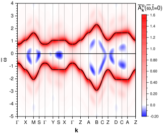
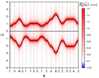
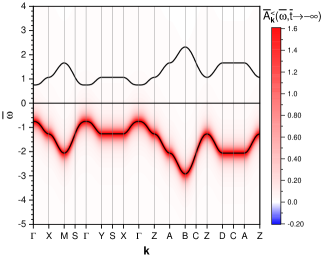
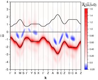
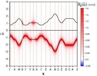
Figure 15: Top and bottom panels: the dimensionless spectral function,$\bar{A}_{\mathbf{k}}^{R}\left(\bar{\omega},t\right)$, and occupied spectral function, $\bar{A}_{\mathbf{k}}^{<}\left(\bar{\omega},t\right)$, respectively, as function of $\omega$ along the main path, for the same pump-pulse and system parameters as the one of Fig. 6. In the left, middle and right panels, the time $t$ is chosen to be well before the application of pump pulse, in the center of the pump pulse ($t=0$), and well after the application of pump pulse, respectively. The black solid curves show the equilibrium bands. The numerical value of $0^{+}$ has been chosen to be $0.2\Delta/\hbar$.

Appendix C Out-of-Equilibrium Spectral Functions

To obtain the spectral functions, we need the Fourier transformation of the GFs with respect to time, which we perform as follows,

$$G_{\mathbf{k}}^{R,<}\left(\omega,t\right) =\int_{-\infty}^{+\infty}d\tau e^{i\omega\tau-0^{+}\left|\tau\right|}G_{\mathbf{k}}^{R,<}\left(t+\frac{\tau}{2},t-\frac{\tau}{2}\right),$$ (109)

where $0^{+}$ is an infinitesimal convergence factor. Then, the retarded spectral function is given by

$$A_{\mathbf{k}}^{R}\left(\omega,t\right)=-\frac{1}{\pi}\imaginary\left[\Tr G_{\mathbf{k}}^{R}\left(\omega,t\right)\right],$$ (110)

while the lesser spectral function is defined as

$$A_{\mathbf{k}}^{<}\left(\omega,t\right)=\frac{1}{2\pi}\imaginary\left[\Tr G_{\mathbf{k}}^{<}\left(\omega,t\right)\right].$$ (111)

In Fig. 15 top and bottom panels, we report the dimensionless retarded and lesser functions, $\bar{A}_{\mathbf{k}}^{R,<}\left(\bar{\omega},t\right)=A_{\mathbf{k}}^{R,<}\left(\bar{\omega},t\right)\Delta/\hbar$ , respectively, as function of $\bar{\omega}$ along the main path, for the same pump-pulse and system parameters as the ones of Fig. 6. In the left, middle and right panels, the time $t$ is chosen to be well before the application of the pump pulse, in the center of the pump pulse ($t=0$), and well after the application of pump pulse, respectively. Clearly, during the application of the pump pulse, the spectral functions, $\bar{A}_{\mathbf{k}}^{R,<}\left(\bar{\omega},t\right)$, become negative and lose their original physical interpretations.

Obviously, in the absence of the pump pulse (both before and after its application), the spectral function gives correct information about the energy bands of the system. The left panel of Fig. 15 can be directly compared to Fig. 3 and the only difference to be acknowledged is that, in the former, the band broadening originates from the finite numerical value of $0^{+}$, while, in the latter, it originates from the finite FWHM of the probe pulse. After the application of the pump pulse, the bands recover their equilibrium shape as it can be seen by comparing the top-right panel of Fig. 15 to its top-left panel. On the other hand, the occupied spectral function (see bottom-right panel of Fig. 15) shows that at some k points we have residual excitations similarly to what is reported in the top panel of Fig. 7.

References

- Brabec and Krausz [2000] T. Brabec and F. Krausz, Reviews of Modern Physics 72, 545 (2000).
- Krausz and Ivanov [2009] F. Krausz and M. Ivanov, Reviews of modern physics 81, 163 (2009).
- Krausz and Stockman [2014] F. Krausz and M. I. Stockman, Nature Photonics 8, 205 (2014).
- Calegari et al. [2016] F. Calegari, G. Sansone, S. Stagira, C. Vozzi, and M. Nisoli, Journal of Physics B: Atomic, Molecular and Optical Physics 49, 062001 (2016).
- Borrego-Varillas et al. [2022] R. Borrego-Varillas, M. Lucchini, and M. Nisoli, Reports on Progress in Physics 85, 066401 (2022).
- Zürch et al. [2017a] M. Zürch, H.-T. Chang, L. J. Borja, P. M. Kraus, S. K. Cushing, A. Gandman, C. J. Kaplan, M. H. Oh, J. S. Prell, D. Prendergast, C. D. Pemmaraju, D. M. Neumark, and S. R. Leone, Nature Communications 8, 15734 (2017a).
- Zürch et al. [2017b] M. Zürch, H.-T. Chang, P. M. Kraus, S. K. Cushing, L. J. Borja, A. Gandman, C. J. Kaplan, M. H. Oh, J. S. Prell, D. Prendergast, C. D. Pemmaraju, D. M. Neumark, and S. R. Leone, Structural Dynamics 4, 044029 (2017b).
- Kaplan et al. [2018] C. J. Kaplan, P. M. Kraus, A. D. Ross, M. Zürch, S. K. Cushing, M. F. Jager, H.-T. Chang, E. M. Gullikson, D. M. Neumark, and S. R. Leone, Phys. Rev. B 97, 205202 (2018).
- Perfetti et al. [2008] L. Perfetti, P. A. Loukakos, M. Lisowski, U. Bovensiepen, M. Wolf, H. Berger, S. Biermann, and A. Georges, New Journal of Physics 10, 053019 (2008).
- Schmitt et al. [2008] F. Schmitt, P. S. Kirchmann, U. Bovensiepen, R. G. Moore, L. Rettig, M. Krenz, J.-H. Chu, N. Ru, L. Perfetti, D. Lu, et al., Science 321, 1649 (2008).
- von der Linde et al. [1995] D. von der Linde, T. Engers, G. Jenke, P. Agostini, G. Grillon, E. Nibbering, A. Mysyrowicz, and A. Antonetti, Physical Review A 52, R25 (1995).
- Norreys et al. [1996] P. A. Norreys, M. Zepf, S. Moustaizis, A. P. Fews, J. Zhang, P. Lee, M. Bakarezos, C. N. Danson, A. Dyson, P. Gibbon, P. Loukakos, D. Neely, F. N. Walsh, J. S. Wark, and A. E. Dangor, Phys. Rev. Lett. 76, 1832 (1996).
- Chin et al. [2001] A. H. Chin, O. G. Calderón, and J. Kono, Physical Review Letters 86, 3292 (2001).
- Ghimire et al. [2011] S. Ghimire, A. D. DiChiara, E. Sistrunk, P. Agostini, L. F. DiMauro, and D. A. Reis, Nature physics 7, 138 (2011).
- Luu et al. [2015] T. T. Luu, M. Garg, S. Y. Kruchinin, A. Moulet, M. T. Hassan, and E. Goulielmakis, Nature 521, 498 (2015).
- Han et al. [2016] S. Han, H. Kim, Y. W. Kim, Y.-J. Kim, S. Kim, I.-Y. Park, and S.-W. Kim, Nature communications 7, 13105 (2016).
- Borja et al. [2016] L. J. Borja, M. Zürch, C. D. Pemmaraju, M. Schultze, K. Ramasesha, A. Gandman, J. S. Prell, D. Prendergast, D. M. Neumark, and S. R. Leone, J. Opt. Soc. Am. B 33, C57 (2016).
- You et al. [2017] Y. S. You, D. A. Reis, and S. Ghimire, Nature physics 13, 345 (2017).
- Liu et al. [2017] H. Liu, Y. Li, Y. S. You, S. Ghimire, T. F. Heinz, and D. A. Reis, Nature Physics 13, 262 (2017).
- Jiang et al. [2019] S. Jiang, S. Gholam-Mirzaei, E. Crites, J. E. Beetar, M. Singh, R. Lu, M. Chini, and C. Lin, Journal of Physics B: Atomic, Molecular and Optical Physics 52, 225601 (2019).
- Schultze et al. [2013] M. Schultze, E. M. Bothschafter, A. Sommer, S. Holzner, W. Schweinberger, M. Fiess, M. Hofstetter, R. Kienberger, V. Apalkov, V. S. Yakovlev, et al., Nature 493, 75 (2013).
- Stojchevska et al. [2014] L. Stojchevska, I. Vaskivskyi, T. Mertelj, P. Kusar, D. Svetin, S. Brazovskii, and D. Mihailovic, Science 344, 177 (2014).
- Schultze et al. [2014] M. Schultze, K. Ramasesha, C. Pemmaraju, S. Sato, D. Whitmore, A. Gandman, J. S. Prell, L. Borja, D. Prendergast, K. Yabana, et al., Science 346, 1348 (2014).
- Lucchini et al. [2016] M. Lucchini, S. A. Sato, A. Ludwig, J. Herrmann, M. Volkov, L. Kasmi, Y. Shinohara, K. Yabana, L. Gallmann, and U. Keller, Science 353, 916 (2016).
- Mashiko et al. [2016] H. Mashiko, K. Oguri, T. Yamaguchi, A. Suda, and H. Gotoh, Nature physics 12, 741 (2016).
- Zürch et al. [2017] M. Zürch, H.-T. Chang, P. M. Kraus, S. K. Cushing, L. J. Borja, A. Gandman, C. J. Kaplan, M. H. Oh, J. S. Prell, D. Prendergast, et al., Structural Dynamics 4, 044029 (2017).
- Schlaepfer et al. [2018] F. Schlaepfer, M. Lucchini, S. A. Sato, M. Volkov, L. Kasmi, N. Hartmann, A. Rubio, L. Gallmann, and U. Keller, Nature Physics 14, 560 (2018).
- Kaplan et al. [2019] C. J. Kaplan, P. M. Kraus, E. M. Gullikson, L. J. Borja, S. K. Cushing, M. Zürch, H.-T. Chang, D. M. Neumark, and S. R. Leone, J. Opt. Soc. Am. B 36, 1716 (2019).
- Geneaux et al. [2019] R. Geneaux, H. J. Marroux, A. Guggenmos, D. M. Neumark, and S. R. Leone, Philosophical Transactions of the Royal Society A 377, 20170463 (2019).
- Inzani et al. [2022] G. Inzani, L. Adamska, A. Eskandari-asl, N. D. Palo, G. L. Dolso, B. Moio, L. J. D’Onofrio, A. Lamperti, A. Molle, R. Borrego-Varillas, M. Nisoli, S. Pittalis, C. A. Rozzi, A. Avella, and M. Lucchini, arXiv preprint arXiv:2212.02157 (2022).
- Neufeld et al. [2023] O. Neufeld, N. Tancogne-Dejean, U. De Giovannini, H. Hübener, and A. Rubio, npj Computational Materials 9, 39 (2023).
- Rohwer et al. [2011] T. Rohwer, S. Hellmann, M. Wiesenmayer, C. Sohrt, A. Stange, B. Slomski, A. Carr, Y. Liu, L. M. Avila, M. Kalläne, et al., Nature 471, 490 (2011).
- Smallwood et al. [2012] C. L. Smallwood, J. P. Hinton, C. Jozwiak, W. Zhang, J. D. Koralek, H. Eisaki, D.-H. Lee, J. Orenstein, and A. Lanzara, Science 336, 1137 (2012).
- Hellmann et al. [2012] S. Hellmann, T. Rohwer, M. Kalläne, K. Hanff, C. Sohrt, A. Stange, A. Carr, M. Murnane, H. Kapteyn, L. Kipp, et al., Nature communications 3, 1069 (2012).
- Papalazarou et al. [2012] E. Papalazarou, J. Faure, J. Mauchain, M. Marsi, A. Taleb-Ibrahimi, I. Reshetnyak, A. van Roekeghem, I. Timrov, N. Vast, B. Arnaud, and L. Perfetti, Phys. Rev. Lett. 108, 256808 (2012).
- Wang et al. [2013] Y. Wang, H. Steinberg, P. Jarillo-Herrero, and N. Gedik, Science 342, 453 (2013).
- Johannsen et al. [2013] J. C. Johannsen, S. Ulstrup, F. Cilento, A. Crepaldi, M. Zacchigna, C. Cacho, I. C. E. Turcu, E. Springate, F. Fromm, C. Raidel, T. Seyller, F. Parmigiani, M. Grioni, and P. Hofmann, Phys. Rev. Lett. 111, 027403 (2013).
- Rameau et al. [2016] J. Rameau, S. Freutel, A. Kemper, M. A. Sentef, J. Freericks, I. Avigo, M. Ligges, L. Rettig, Y. Yoshida, H. Eisaki, et al., Nature communications 7, 13761 (2016).
- Reimann et al. [2018] J. Reimann, S. Schlauderer, C. Schmid, F. Langer, S. Baierl, K. Kokh, O. Tereshchenko, A. Kimura, C. Lange, J. Güdde, et al., Nature 562, 396 (2018).
- Smith and Traum [1975] N. Smith and M. Traum, Physical Review B 11, 2087 (1975).
- Himpsel and Eastman [1978] F. J. Himpsel and D. E. Eastman, Phys. Rev. B 18, 5236 (1978).
- Kampf and Schrieffer [1990] A. P. Kampf and J. R. Schrieffer, Phys. Rev. B 42, 7967 (1990).
- Smith and Kevan [1991] K. E. Smith and S. D. Kevan, Progress in solid state chemistry 21, 49 (1991).
- Damascelli et al. [2003] A. Damascelli, Z. Hussain, and Z.-X. Shen, Reviews of modern physics 75, 473 (2003).
- Hüfner [2013] S. Hüfner, Photoelectron spectroscopy: principles and applications (Springer Science & Business Media, 2013).
- Sobota et al. [2021] J. A. Sobota, Y. He, and Z.-X. Shen, Reviews of Modern Physics 93, 025006 (2021).
- Bovensiepen and Kirchmann [2012] U. Bovensiepen and P. S. Kirchmann, Laser & Photonics Reviews 6, 589 (2012).
- Smallwood et al. [2016] C. L. Smallwood, R. A. Kaindl, and A. Lanzara, EPL (Europhysics Letters) 115, 27001 (2016).
- Zhou et al. [2018] X. Zhou, S. He, G. Liu, L. Zhao, L. Yu, and W. Zhang, Reports on Progress in Physics 81, 062101 (2018).
- Weinelt [2002] M. Weinelt, Journal of Physics: Condensed Matter 14, R1099 (2002).
- Echenique et al. [2004] P. M. Echenique, R. Berndt, E. V. Chulkov, T. Fauster, A. Goldmann, and U. Höfer, Surface Science Reports 52, 219 (2004).
- Sobota et al. [2013] J. A. Sobota, S.-L. Yang, A. F. Kemper, J. J. Lee, F. T. Schmitt, W. Li, R. G. Moore, J. G. Analytis, I. R. Fisher, P. S. Kirchmann, T. P. Devereaux, and Z.-X. Shen, Phys. Rev. Lett. 111, 136802 (2013).
- Broers and Mathey [2022] L. Broers and L. Mathey, Physical Review Research 4, 013057 (2022).
- Avigo et al. [2013] I. Avigo, R. Cortés, L. Rettig, S. Thirupathaiah, H. S. Jeevan, P. Gegenwart, T. Wolf, M. Ligges, M. Wolf, J. Fink, et al., Journal of Physics: Condensed Matter 25, 094003 (2013).
- Yang et al. [2015] S.-L. Yang, J. A. Sobota, D. Leuenberger, Y. He, M. Hashimoto, D. H. Lu, H. Eisaki, P. S. Kirchmann, and Z.-X. Shen, Phys. Rev. Lett. 114, 247001 (2015).
- De Giovannini et al. [2013] U. De Giovannini, G. Brunetto, A. Castro, J. Walkenhorst, and A. Rubio, ChemPhysChem 14, 1298 (2013).
- De Giovannini et al. [2016] U. De Giovannini, H. Hubener, and A. Rubio, Nano letters 16, 7993 (2016).
- Wopperer et al. [2017] P. Wopperer, U. De Giovannini, and A. Rubio, The European Physical Journal B 90, 1 (2017).
- De Giovannini et al. [2017] U. De Giovannini, H. Hübener, and A. Rubio, Journal of chemical theory and computation 13, 265 (2017).
- Pemmaraju et al. [2018] C. D. Pemmaraju, F. D. Vila, J. J. Kas, S. A. Sato, J. J. Rehr, K. Yabana, and D. Prendergast, Computer Physics Communications 226, 30 (2018).
- Tancogne-Dejean and Rubio [2018] N. Tancogne-Dejean and A. Rubio, Science advances 4, eaao5207 (2018).
- De Giovannini et al. [2018] U. De Giovannini, A. Castro, et al., Attosecond Molecular Dynamics 13, 424 (2018).
- Armstrong et al. [2021] G. S. Armstrong, M. A. Khokhlova, M. Labeye, A. S. Maxwell, E. Pisanty, and M. Ruberti, The European Physical Journal D 75, 209 (2021).
- Schüler et al. [2021] M. Schüler, J. A. Marks, Y. Murakami, C. Jia, and T. P. Devereaux, Physical Review B 103, 155409 (2021).
- Freericks et al. [2006] J. K. Freericks, V. M. Turkowski, and V. Zlatić, Phys. Rev. Lett. 97, 266408 (2006).
- Aoki et al. [2014] H. Aoki, N. Tsuji, M. Eckstein, M. Kollar, T. Oka, and P. Werner, Reviews of Modern Physics 86, 779 (2014).
- Golež et al. [2019] D. Golež, L. Boehnke, M. Eckstein, and P. Werner, Physical Review B 100, 041111(R) (2019).
- Eckstein [2021] M. Eckstein, Journal of Electron Spectroscopy and Related Phenomena 253, 147108 (2021).
- DÓnofrio et al. [2022] L. J. DÓnofrio, A. Eskandari-asl, and A. Avella, Journal of Magnetism and Magnetic Materials 546, 168785 (2022).
- Sato et al. [2018] S. A. Sato, M. Lucchini, M. Volkov, F. Schlaepfer, L. Gallmann, U. Keller, and A. Rubio, Physical Review B 98, 035202 (2018).
- Mancini and Avella [2004] F. Mancini and A. Avella, Advances in Physics 53, 537 (2004).
- Avella and Mancini [2007] A. Avella and F. Mancini, Phys. Rev. B 75, 134518 (2007).
- Avella and Mancini [2012] A. Avella and F. Mancini, The composite operator method (com), in Strongly Correlated Systems: Theoretical Methods, edited by A. Avella and F. Mancini (Springer Berlin Heidelberg, Berlin, Heidelberg, 2012) pp. 103–141.
- Avella [2014a] A. Avella, The European Physical Journal B 87, 1 (2014a).
- Avella [2014b] A. Avella, Advances in Condensed Matter Physics 2014, 515698 (2014b).
- Di Ciolo and Avella [2018] A. Di Ciolo and A. Avella, Condensed Matter Physics 21 (2018).
- Mostofi et al. [2014] A. A. Mostofi, J. R. Yates, G. Pizzi, Y.-S. Lee, I. Souza, D. Vanderbilt, and N. Marzari, Computer Physics Communications 185, 2309 (2014).
- Peierls [1933] R. Peierls, Zeitschrift für Physik 80, 763 (1933).
- Ismail-Beigi et al. [2001] S. Ismail-Beigi, E. K. Chang, and S. G. Louie, Physical Review Letters 87, 087402 (2001).
- Yue and Gaarde [2022] L. Yue and M. B. Gaarde, JOSA B 39, 535 (2022).
- Freericks et al. [2009] J. K. Freericks, H. R. Krishnamurthy, and T. Pruschke, Phys. Rev. Lett. 102, 136401 (2009).
- Sentef et al. [2013] M. Sentef, A. F. Kemper, B. Moritz, J. K. Freericks, Z.-X. Shen, and T. P. Devereaux, Physical Review X 3, 041033 (2013).
- Freericks et al. [2015] J. Freericks, H. Krishnamurthy, M. Sentef, and T. Devereaux, Physica Scripta 2015, 014012 (2015).
- Schüler and Sentef [2021] M. Schüler and M. A. Sentef, Journal of Electron Spectroscopy and Related Phenomena 253, 147121 (2021).