Data-driven decoding of quantum error correcting codes using graph neural networks

Abstract

To leverage the full potential of quantum error-correcting stabilizer codes it is crucial to have an efficient and accurate decoder. Accurate, maximum likelihood, decoders are computationally very expensive whereas decoders based on more efficient algorithms give sub-optimal performance. In addition, the accuracy will depend on the quality of models and estimates of error rates for idling qubits, gates, measurements, and resets, and will typically assume symmetric error channels. In this work, instead, we explore a model-free, data-driven, approach to decoding, using a graph neural network (GNN). The decoding problem is formulated as a graph classification task in which a set of stabilizer measurements is mapped to an annotated detector graph for which the neural network predicts the most likely logical error class. We show that the GNN-based decoder can outperform a matching decoder for circuit level noise on the surface code given only simulated experimental data, even if the matching decoder is given full information of the underlying error model. Although training is computationally demanding, inference is fast and scales approximately linearly with the space-time volume of the code. We also find that we can use large, but more limited, datasets of real experimental data [Google Quantum AI, Nature 614, 676 (2023)] for the repetition code, giving decoding accuracies that are on par with minimum weight perfect matching. The results show that a purely data-driven approach to decoding may be a viable future option for practical quantum error correction, which is competitive in terms of speed, accuracy, and versatility.

I Introduction

Quantum Error Correction (QEC) is foreseen to be a vital component in the development of practical quantum computing Shor (1995); Steane (1996); Gottesman (1997); Terhal (2015); Girvin (2021). The need for QEC arises due to the susceptibility of quantum information to noise, which can rapidly accumulate and corrupt the final output. Unlike noise mitigation schemes where errors are reduced by classical post-processing Kim et al. (2023); Temme et al. (2017); Li and Benjamin (2017), QEC methods encode quantum information in a way that allows for the detection and correction of errors without destroying the information itself. A prominent framework for this are topological stabilizer codes, such as the surface code, for which the logical failure rates can be systematically suppressed by increasing the size of the code if the intrinsic error rates are below some threshold value Bravyi and Kitaev (1998); Dennis et al. (2002a); Kitaev (2003); Raussendorf and Harrington (2007); Fowler et al. (2012).

Stabilizer codes are based on a set of commutative, typically local, measurements that project an $n$-qubit state to a lower dimensional code space representing one or more logical qubits. Errors take the state out of the code space and are then indicated by a syndrome, corresponding to stabilizer violations. The syndrome needs to be interpreted in order to gauge whether a logical bit or phase flip may have been incurred on the logical qubit. Interpreting the syndrome, to predict the most likely logical error, requires both a decoder algorithm and, traditionally, a model of the qubit error channels. The fact that measurements may themselves be noisy, makes this interpretation additionally challenging Dennis et al. (2002a); Fowler et al. (2012).

Efforts are under way to realize stabilizer codes experimentally using various qubit architectures Kelly et al. (2015); Takita et al. (2017); Wootton and Loss (2018); Wootton (2020); Andersen et al. (2020); Satzinger et al. (2021); Egan et al. (2021); Chen et al. (2021); Erhard et al. (2021); Ryan-Anderson et al. (2021); Marques et al. (2021); Postler et al. (2022); Krinner et al. (2022); Bluvstein et al. (2022); Google Quantum AI (2023); Moses et al. (2023); Sundaresan et al. (2023). In Google Quantum AI (2023), code distance 3 and 5 surface codes were implemented, using 17 and 49 superconducting qubits, respectively. After initialization of the qubits, repeated stabilizer measurements are performed over a given number of cycles capped by a final round of single qubit measurements. The results are then compared with the initial state to determine whether errors have caused a logical bit- (or phase-) error. The decoder analyses the collected sets of syndrome measurements in post-processing, where the fraction of correct predictions gives a measure of the logical accuracy. The better the decoder, the higher the coherence time of the logical qubit, and in Google Quantum AI (2023) a computationally costly tensor network based decoder was used to maximize the logical fidelity of the distance 5 code compared to the distance 3 code. However, with the objective of moving from running and benchmarking a quantum memory to using it for universal quantum computation, it will be necessary to do error correction both with high accuracy and in real time.

In the present work, we explore the viability of using a purely data-driven approach to decoding, based on the potential of generating large amounts of experimental data. We use a graph neural network (GNN) which is well suited for addressing this type of data. Namely, a single data point, as in Google Quantum AI (2023), consists of a set of “detectors”, i.e., changes in stabilizer measurements from one cycle to the next, together with a label indicating the measured logical bit- or phase-flip error. This can be represented as a labeled graph with nodes that are annotated by the information on the type of stabilizer and the space-time position of the detector, as shown in Figure 1. The maximum degree of the graph can be capped based on removing edges between distant detectors, keeping only a fixed maximum number of neighboring nodes. The latter ensures that each network layer in the GNN (see Figure 2) performs a number of matrix multiplications that scales linearly with the number of nodes, i.e., linearly with the number of stabilizer measurements and the overall error rate. We have trained this decoder on simulated experimental data for the surface code using Stim Gidney (2021) as well as real experimental data on the repetition code Google Quantum AI (2023). For both of these, the decoder is on par with, or outperforms, the state-of-the-art matching decoder Higgott (2021), suggesting that with sufficient data and a suitable neural network architecture, model-free machine learning based decoders trained on experimental data can be competitive for future implementations of quantum error-correcting stabilizer codes.

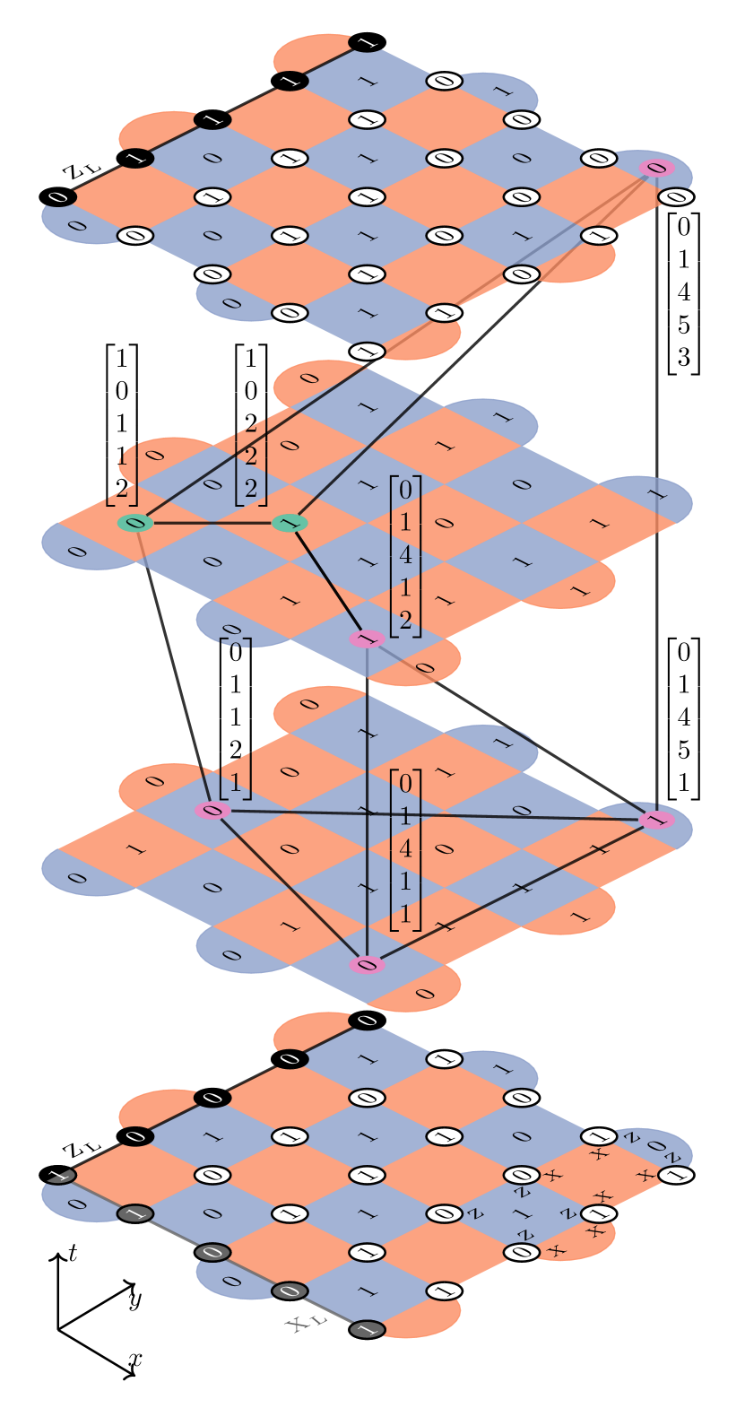
Figure 1: Memory experiment on the distance $d=5$ surface code. Data qubit initialization is followed by $d_{t}=2$ stabilizer measurement rounds and a final data qubit measurement round. Data qubits are on the vertices of plaquettes (circles, shown in the bottom and top planes). Ancilla qubits (not shown) at the center of plaquettes provide stabilizer measurements outcomes. The detector graph has nodes corresponding to changes in stabilizers from the previous time step. (Not all edges shown.) Nodes are annotated by the type of stabilizer and the space-time coordinate. The label, here $\lambda_{Z}=1$, corresponding to a change of $\langle Z_{L}\rangle$, measured along the northwest edge. Also shown, bottom layer, are some example stabilizers, and the logical $X_{L}$ (not measured).

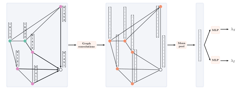
Figure 2: Schematic of the GNN decoder. It takes as input an annotated detector graph, c.f. Figure 1. Several layers of graph convolutional operations (following Eqn. 3) transform each node feature vector. (The empty circle shows the message passing to this particular node from neighboring nodes on the graph.) Next, a mean-pooling operation averages all the node feature vectors into a single graph embedding, which is independent of the size of the graph. Finally, the latter is passed through two separate dense networks to give two binary class predictors, corresponding to the logical $X$ and $Z$ labels, respectively. (For details see Appendix A.)

II Stabilizer codes and decoding

A stabilizer code is defined through a set of commuting operators constructed from products of Pauli operators acting on a Hilbert space of $n$ data qubits Gottesman (1997). With $n_{S}$ independent stabilizers the Hilbert space is split into sectors of dimension $2^{n-n_{S}}$, specified by the parity under each stabilizer. For concreteness we will consider the case $n_{S}=n-1$, such that each of the sectors represent a single qubit degree of freedom. Each syndrome measurement is performed with the help of an ancilla qubit following a small entangling circuit with the relevant data qubits. The measured state of the ancilla qubits provide a syndrome $S=\{s_{i},i=1,...,n_{S}\,|\in 0,1\}$, and projects the density matrix of the $n$ qubit state into a single 2-dimensional block, a Pauli frame Knill (2005); de Beaudrap and Horsman (2020). Given uncertainties in the measurements, a number of rounds are typically performed before the information is interpreted by means of a decoder.

Defining a pair of anticommuting operators $Z_{L}$ and $X_{L}$ that commute with the stabilizer group, provides the logical computational space through $Z_{L}|0\rangle_{L}=|0\rangle_{L}$ and $|1\rangle_{L}=X_{L}|0\rangle_{L}$. Assuming a fixed pair of logical operators for a given code defines the corresponding logical states in each Pauli frame. Thus, a number of subsequent rounds of stabilizer measurements, during which the code is affected by decoherence, transforms the density matrix from the initial state $\rho=\sum_{i,j\in\{0,1\}}\rho_{ij}|i\rangle_{L}\langle j|_{L}$ to the final state $\rho^{\prime}=\sum_{i,j\in\{0,1\}}\rho^{\prime}_{ij}|i\rangle^{\prime}_{L}\langle j|^{\prime}_{L}$, where $|0/1\rangle_{L}$ ($|0/1\rangle^{\prime}_{L}$) are the logical qubit states in the initial (final) Pauli frame. The logical error channels are approximated by

$$\rho \rightarrow\rho^{\prime}=\epsilon_{L}(\rho_{L})$$

$$= (1-P)\rho+P_{X}X_{L}\rho X_{L}+P_{Z}Z_{L}\rho Z_{L}+P_{Y}Y_{L}\rho Y_{L}\,,$$

with $Y_{L}=-iZ_{L}X_{L}$ and $P=\sum_{i=X,Y,Z}P_{i}$. In general there may be additional non-symmetric channels (see for example Satzinger et al. (2021)), but we will assume that the data (as in Google Quantum AI (2023)) does not resolve such channels.

The probabilities of logical error, $P_{i}$, will be quantified by the complete set of syndrome measurements and depend on single and multi-qubit error channels as well as measurement and reset errors. It is the task of the decoder to quantify these in order to maximize the effectiveness of the error correction. Traditionally this is done through computational algorithms that use a specific error model. The framework that most decoders are based on uses independent and identically distributed symmetric noise acting on individual qubits, possibly, for circuit-level noise, complemented by two-qubit gate errors, faulty measurements and ancilla qubit reset errors. Maximum-likelihood decoders Wootton and Loss (2012); Hutter et al. (2014); Bravyi et al. (2014); Hammar et al. (2022); Pryadko (2020); Chubb (2021) aim to explicitly account for all possible error configurations that are consistent with the measured syndromes, with their respective probabilities given by the assumed error model. The full set of error configurations fall in four different cosets that map to each other by the logical operators of the code, thus directly providing an estimate of the probabilities $P_{i}$ that is limited only by the approximations involved in the calculation and the error model. Even though such decoders may be useful for benchmarking and optimizing the theoretical performance of stabilizer codes Google Quantum AI (2023), they are computationally too demanding for real time operation, even for small codes.

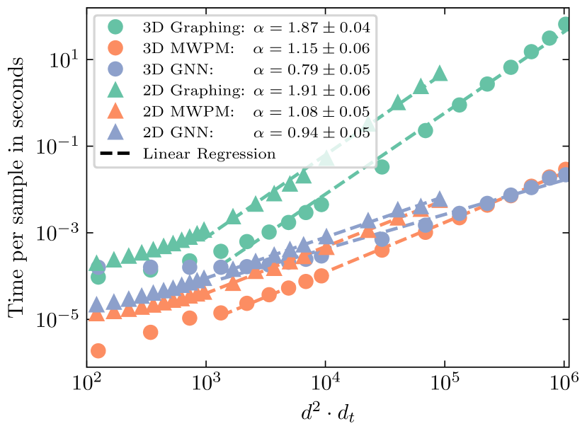
Figure 8: Scaling of average decoding time per syndrome versus code volume $d^{2}d_{t}$ for GNN and MWPM. Perfect stabilizer measurements sampled at $p=0.05$ (labeled 2D) and circuit level noise sampled at $p=10^{-3}$ (labeled 3D). Dotted lines show a regression for $d\geq 31$ and $d\geq 11$ for 2D and 3D, respectively, according to the ansatz: $T=C\cdot(d^{2}\cdot d_{t})^{\alpha}$, with the GNN showing sub-linear scaling. The average graph construction time per sample is shown in green.

The more standard decoders instead are based on the minimum weight perfect matching (MWPM) algorithm Edmonds (1965); Dennis et al. (2002b); Wang et al. (2010, 2011); Fowler (2015); Brown (2022). Such a decoder aims to find the single, most likely, configuration of single qubit errors consistent with the set of measured stabilizers. Detectors are mapped to nodes of a graph with edges that are weighted by the probability of the pair of nodes. For codes where nodes appear in pairs (such as the repetition or surface code), the most likely error corresponds to pairwise matching such that the total weight of the edges is minimized. This algorithm is fast, in practice scaling approximately linearly with the size of the graph (see Figure 8). Nevertheless, it has several short-comings that limits accuracy and applicability: 1) Approximate handling of crossing edges (such as coinciding X and Z errors) means that the effective error model is oversimplified. 2) Except at very low error rates, degeneracies of less likely error configurations are ignored. 3) For models where a single error may give rise to more than two detector events, more sophisticated algorithms are needed Delfosse (2014); Stephens (2014); Delfosse and Nickerson (2021); Tuckett et al. (2020); Sahay and Brown (2022); Berent et al. (2023); Benhemou et al. (2023). These shortcomings can be partially addressed by more sophisticated approaches such as counting multiplicity or using belief propagation Delfosse and Tillich (2014); Criger and Ashraf (2018); Higgott et al. (2022); Caune et al. (2023), but often at the cost of added computational complexity. Other examples of decoder algorithms are based on decoding from small to large scale, such as cellular-automata Herold et al. (2015); Kubica and Preskill (2019); Miguel et al. (2023), renormalization group Duclos-Cianci and Poulin (2010), or union-find Delfosse and Nickerson (2021); Huang et al. (2020). The latter, in particular, is very efficient, but at the cost of sub-optimal performance.

II.1 Related work

A number of different deep learning based decoder algorithms have also been formulated, based on supervised learning, reinforcement learning, and genetic neural algorithms Torlai and Melko (2017); Krastanov and Jiang (2017); Varsamopoulos et al. (2017); Baireuther et al. (2018); Breuckmann and Ni (2018); Baireuther et al. (2019); Chamberland and Ronagh (2018); Nautrup et al. (2019); Maskara et al. (2019); Ni (2020); Sweke et al. (2020); Andreasson et al. (2019); Colomer et al. (2020); Fitzek et al. (2020); Gicev et al. (2021); Bhoumik et al. (2021); Théveniaut and van Nieuwenburg (2021); Meinerz et al. (2022); Overwater et al. (2022); Chamberland et al. (2022); Zhang et al. (2023). Focusing on the works on the surface code and based on supervised learning, these can roughly be separated according to whether they primarily consider perfect stabilizers Torlai and Melko (2017); Krastanov and Jiang (2017); Varsamopoulos et al. (2017); Ni (2020); Gicev et al. (2021); Bhoumik et al. (2021); Overwater et al. (2022), or include measurement noise or circuit-level noise Baireuther et al. (2018); Chamberland and Ronagh (2018); Meinerz et al. (2022); Chamberland et al. (2022); Zhang et al. (2023), and whether they are purely data-driven Torlai and Melko (2017); Varsamopoulos et al. (2017); Baireuther et al. (2018); Chamberland and Ronagh (2018); Overwater et al. (2022); Zhang et al. (2023) or involve some auxiliary, model-informed, algorithm or multi-step reduction of decoding Krastanov and Jiang (2017); Chamberland et al. (2022); Ni (2020); Gicev et al. (2021); Bhoumik et al. (2021); Meinerz et al. (2022).

The present work is in the category, realistic (circuit-level) noise, and purely data-driven. It is distinguished primarily in that we 1) Use graph neural networks and graph structured data, and 2) Train and test the neural network decoder on real experimental data. In addition, as in several of the earlier works Chamberland and Ronagh (2018); Baireuther et al. (2018, 2019), we emphasize the use of a model-free, purely data-driven, approach. By using experimental stabilizer data, the approximations of traditional model-based decoder algorithms can be avoided. The fact that the real error channels at the qubit level may be asymmetric, due to amplitude damping, have long-range correlations, or involve leakage outside the computational space, is intrinsic to the data. This is also in contrast to other data-driven approaches Wagner et al. (2022); Chen et al. (2022); Wagner et al. (2023); Google Quantum AI (2023); Chen et al. (2021) that use stabilizer data to learn the detailed Pauli channels, optimize a decoder algorithm through the edge weights of a matching decoder, or the individual qubit and measure error rates of a tensor network based decoder, as these are all constrained by a specific error model.

II.2 Repetition code and surface code

The decoder formalism that we present in this work can be applied to any stabilizer code, requiring only a dataset of measured (or simulated) stabilizers, together with the logical outcomes. Nevertheless, to keep to the core issues of training and performance we consider only two standard scalable stabilizer codes: the repetition code and the surface code.

The repetition code is defined on a one-dimensional grid of qubits with neighboring pair-wise $Z_{i}\otimes Z_{i+1}$ stabilizers. In the Pauli frame with all $+1$ stabilizers, the code words are $|0\rangle_{L}=|0\rangle^{\otimes n}$ and $|1\rangle_{L}=|1\rangle^{\otimes n}$. Consider a logical qubit state $|\psi\rangle=\alpha|0\rangle_{L}+\beta|1\rangle_{L}$, with complex amplitudes $|\alpha|^{2}+|\beta|^{2}=1$. The logical bit-flip operator is given by $X_{L}=\bigotimes_{i}X_{i}$, which sets the code distance $d_{X}=n$. Assuming perfect stabilizer measurements and independent and identically distributed single qubit bit-flip error probabilities, decoding the repetition code is trivial. For any set of stabilizer violations, i.e., odd parity outcomes, there are only two consistent configurations of errors that map to each other by acting with $X_{L}$. A decoder (maximum-likelihood in the case of this simple error model) would suggest the one with fewer errors. The repetition code, set up to detect bit-flip errors, is insensitive to phase flip errors, as is clear from the fact that a phase-flip ($Z$) error on a single qubit also gives a phase-flip error ($\beta\rightarrow-\beta$) on the logical qubit, corresponding to a code distance $d_{Z}=1$. To detect and correct both bit- and phase-flip errors we need a more potent code, the most promising of which may be the surface code.

We consider the qubit-efficient “rotated” surface code Bombin and Martin-Delgado (2007); Tomita and Svore (2014); Tuckett et al. (2019) (see Figure 1), constructed from weight-4, $Z^{\otimes 4}$ and $X^{\otimes 4}$, stabilizers (formally stabilizer generators), with complementary weight-2 stabilizers on the boundary. On a square grid of $d\times d$ data qubits, the $d^{2}-1$ stabilizers give one logical qubit. We define the logical operator $X_{L}$ as a string of $X$’s on the southwest edge, and a string of $Z$’s on the northwest edge, as shown in Figure 1. These are the two (unique up to products of stabilizers) lowest weight operators that commute with the stabilizer group, without being part of said group.

Stabilizer measurements are performed by means of entangling circuits between the data qubits and an ancilla qubit. Assuming hardware with one ancilla qubit per stabilizer, and the appropriate gate schedule, these can all be measured simultaneously, corresponding to one round of stabilizer measurements.

II.3 Memory experiments on the surface code

To train and test our decoder we consider a real or simulated experiment, illustrated schematically in Figure 1, to benchmark a surface code as a quantum memory. The following procedure can be used for any stabilizer code:

• Initialize the individual qubits: Data qubits in a fixed or random configuration in the computational basis $|0\rangle$ and $|1\rangle$. Ancilla qubits in $|0\rangle$. The initial data qubit configuration is viewed as a 0’th round of measurements that initialize the $Z$-stabilizers. This also corresponds to an effective measurement $\langle Z_{L}\rangle_{t=0}=\prod_{i\in Z_{L}}Z_{i}=\pm 1$. (Northwest row of qubits in Figure 1.)

• A first round, $t=1$, of actual stabilizer measurements is performed. The Z-stabilizers are determined, up to bit-flip errors, by the 0’th round. Hence, the difference between the two provides the first round of Z-detectors. The X-stabilizers have randomized outcome, projecting to an even or odd parity state over the four (or two) qubits in the Hadamard ($|+\rangle$, $|-\rangle$) basis. The value of these stabilizers form the reference for subsequent error detecting measurements of the X-stabilizers. Ancilla qubits are reset to 0 after this and subsequent rounds.

• Subsequent rounds $t=2,...,d_{t}$ of Z and X stabilizer measurements provide the input for corresponding detectors based on changes from the previous round.

• Finally, data qubits are measured individually in the Z-basis, which provides a final measurement, $\langle Z_{L}\rangle_{t=d_{t}+1}$. These also provide a final round of Z-stabilizers, which, since they are provided by the actual qubit outcomes rather than by measuring an ancilla, are perfect stabilizers by definition.

The outlined experiment provides a single data point $D=(\{V_{Z}\},\{V_{X}\},\lambda_{Z})$ consisting of set of Z-detectors $\{V_{Z}\}$, over $d_{t}+1$ cycles and a set of X-detectors $\{V_{X}\}$ over $d_{t}-1$ cycles. In addition to the stabilizer type, each detector is tagged with its space-time coordinate, $(x,y,t)$, with $0\leq x,y\leq d$ and $1\leq t\leq d_{t}\pm 1$ for $Z$ and $X$ detectors respectively. The logical label is given by

$$\lambda_{Z}=\frac{1}{2}|\langle Z_{L}\rangle_{t=0}-\langle Z_{L}\rangle_{t=d_{t}+1}|\in\{0,1\}\,.$$ (2)

The probability of $\lambda_{Z}=1$ is, according to Eqn. II, given by $P_{X}+P_{Y}$, and the probability of $\lambda_{Z}=0$ by $P_{I}+P_{Z}$, corresponding to a logical bit-flip or not.

What has been described is a “memory-Z” experiment Gidney (2021), i.e., one in which we detect logical bit-flips. Qubits are initialized in the computational basis $|0\rangle$ and $|1\rangle$. A “memory-X” experiment prepares the qubits in the Hadamard basis, with the role of X- and Z-stabilizers reversed. Physically, in the lab, one cannot do both experiments in the same run, as $Z_{L}$ and $X_{L}$ do not commute. This also implies that each data point only has one of the two binary labels, $\lambda_{Z}$ or $\lambda_{X}$, even though there is information in the detectors about both labels. The neural network will be constructed to predict both labels for a given set of detectors, which implies that the learning framework is effectively that of semi-supervised learning, with partially labeled data. Thus, in contrast to a matching based decoder, which breaks the surface code detectors into two independent sets with a corresponding graph for each, the GNN decoder can make use of the complete information. This, in addition to the fact that it is not constrained by the limitations of the matching algorithm itself, provides a possible advantage in terms of prediction accuracy.

Additionally, some fraction of the data is incorrectly labeled. This follows from the fact that measured labels will not always be the most likely. In fact, the fraction of incorrectly labeled data corresponds to the logical failure rate that an optimal decoder would provide. For the data that we use, this fraction ranges from marginal (see Figure 4) to quite substantial (see Figure 6), depending in particular on the number of cycles that are decoded, as the logical failure rate grows exponentially with the number of cycles.

We have also assumed that there is no post-processing to remove leakage. Assuming there is some mechanism of relaxation back to the computational qubit subspace, including the last round of measurements, leakage events will be be handled automatically by the neural network decoder, based on the signature they leave in the detector data.

III Graph neural network decoder

A graph neural network (GNN) can be viewed as a trainable message passing algorithm, where information is passed between the nodes through the edges of the graph and processed through a neural network Kipf and Welling (2016); Wu et al. (2020); Dwivedi et al. (2020). The input is data in the form of a graph $G=(V,E)$, with a set of nodes $V=\{i\,|\,i=1,..,N\}$ and edges $E=\{(i,j)\,|\,i\neq j\in V\}$, which is annotated by $n$-dimensional node feature vectors $\vec{X}_{i}$ and edge weights (or vectors) $e_{ij}$. The basic building blocks are the message passing graph convolutional layers, which take a graph as input and outputs an isomorphic graph with transformed feature vectors. Specifically, in this work we have used a standard graph convolution Morris et al. (2021) where for each node the $d_{in}$-dimensional feature vector $\vec{X}_{i}$ is transformed to new feature vector $\vec{X}^{\prime}_{i}$ with dimension $d_{out}$ according to

$$\vec{X}^{\prime}_{i}=\sigma\left(W_{1}\vec{X}_{i}+\sum_{j}e_{ij}W_{2}\vec{X}_{i}\right)\,,$$ (3)

where non-existent edges are indicated by $e_{ij}=0$. Here $W_{1}$ and $W_{2}$ are $d_{out}\times d_{in}$ dimensional trainable weight matrices and $\sigma$ is an element-wise non-linear activation function which includes a $d_{out}$-dimensional trainable bias vector.

For the task at hand, which is graph classification, graph convolutions are followed by a pooling layer that contracts the information to a single vector, a graph embedding, which is independent of the dimension of the graph. We use a simple mean-pooling layer $\vec{X}^{\prime}=N^{-1}\sum_{i}\vec{X}_{i}$. For the classification we use two structurally identical, but independent, standard multi-layer feedforward networks that each end with a single node with sigmoid activation that acts as a binary classifier. The weights and biases of the complete network are trained using stochastic gradient descent with a loss function which is a sum of the binary cross entropy loss of the network output with respect to the binary labels. Since the experimental data, or simulated experimental data, only has one of the two binary labels ($\lambda_{Z}$, $\lambda_{X}$) for each complete detector graph, gradients are only calculated for the provided label.

To avoid overfitting to the training data we employ two different approaches depending on the amount of available data. In using experimental data from Google Quantum AI (2023), we use a two-way split into a training set and a test set. To avoid diminishing the training data further, we do not use a validation set, and instead train for a fixed number of epochs. We observe (see Figure 6) that the test accuracy does not change significantly over a large number of epochs, even though the network continues to overfits.

For the case with simulated experimental data (Figure 4), we avoid overfitting by replacing a substantial fraction (25%) of the data with new data, generated within the training cycle, after each epoch of training. This effectively emulates a much larger dataset, while keeping with the memory limits set by the available hardware. Since the training set is effectively unbounded, the number of unique detector graphs scales as $2^{d_{t}d^{2}}$ and the network cannot overfit. Also here, a fixed test set is used to gauge the performance.

The GNN training and testing is implemented in PyTorch Geometric Fey and Lenssen (2019), simulated data is generated using Stim Gidney (2021), and the MWPM decoding results use Pymatching Higgott (2021). The Adam optimizer is used for stochastic gradient descent, using manual learning rate decrements when the training accuracy has leveled out. Details on the training procedure can be found in Appendix A. Several other graph layers were experimented with, including graph attention for both convolutions Veličković et al. (2017) and pooling Lee et al. (2019); Knyazev et al. (2019), as well as top_k pooling Gao and Ji (2019); Cangea et al. (2018). These were found not to improve results. The width and depth of the final network was arrived at after several rounds of iterations. Naturally, we expect that larger code distances, i.e., larger graphs, will require scaling up the network size. (See also Sec. IV.4)

III.1 Data structure

As discussed previously the data is in a form $D=(\{V_{Z}\},\{V_{X}\},\lambda_{Z/X})$, consisting of a set of detectors $V_{Z/X}$, specified by a space-time coordinate, together with a binary label. Based on this we construct a single graph. Each node corresponds to a detector event, and is annotated by a 5-vector (for the surface code with circuit-level noise) $\vec{X}=(b_{1},b_{2},x,y,t)$ containing the space-time coordinate $(x,y,t)$ and two exclusive binary (one-hot encoded) labels with $\vec{b}=(1,0)$ for an X-stabilizer and $\vec{b}=(0,1)$ for a Z-stabilizer. (The encoding of the type of stabilizer may be superfluous, as it can be deduced from the coordinate.) We initially consider a complete graph, with edge weights given by the inverse square supremum norm between the vertices, $e_{ij}=(\max\{|x_{i}-x_{j}|,|y_{i}-y_{j}|,|t_{i}-t_{j}|\})^{-2}$. This form of the edge weights is motivated by a naive picture of the minimum number of single data qubit measurement errors that would cause a pair of detectors. The main purpose of the weights is to give some measure of locality, in order to prune the graph. Smaller weight edges are removed, leaving only a fixed maximal node degree, which for the results presented in this work was capped at six.

IV Results

The GNN based decoder has been implemented, trained, and tested on the surface code and the repetition code. The main focus is on using simulated or real experimental data, presented in IV.1 and IV.2, respectively. We also present some results on the surface code with perfect stabilizers, IV.3, where we are able to train the network for larger code distances.

IV.1 Surface code with circuit-level noise

We use Stim to generate data with circuit-level noise. Simulated circuits use standard settings for the surface code, containing Hadamard single qubit gates, controlled-Z (CZ) entangling gates, and measure and reset operations. All of these operations, and the idling, contain Pauli noise, scaled by an overall error rate $p$. (See Appendix B.) Datasets of several million graphs are generated, with partial replacement after each epoch of training to avoid overfitting. Figure 3 shows test results evaluated at $p=1.0\cdot 10^{-3}$ for decoders trained with data using an even mix of error rates $p=\{1.0,2.0,3.0,4.0,5.0\}\cdot 10^{-3}$ and memory-Z experiments. The logical failure rate is thus approximately 50% of the true failure rate (up to correlations between failures in $X_{L}$ and $Z_{L}$), but consistent with the type of data that would be experimentally accessible. (We have also tried training and testing with a mix of memory-Z and memory-X experiments, which works as well but takes longer to train to the same accuracy.) The MWPM decoder uses the information provided by the simulated error model to optimize edge weights on the decoding graph, whereas the GNN decoder uses only the data provided by the simulated measurements. Despite this, we find that with sufficient training the GNN decoder outperforms the matching decoder.

A different network is trained for each code distance $d$ and for each number of rounds of stabilizer measurements $d_{t}$. Figure 4 shows a representative plot of the training and validation accuracy, evaluated on the mixed error rate dataset. With an active (in-memory) dataset containing $5\cdot 10^{6}$ and given that 25% is replaced in each epoch, 1000 epochs corresponds to a total of $1.25\,10^{9}$ data points .

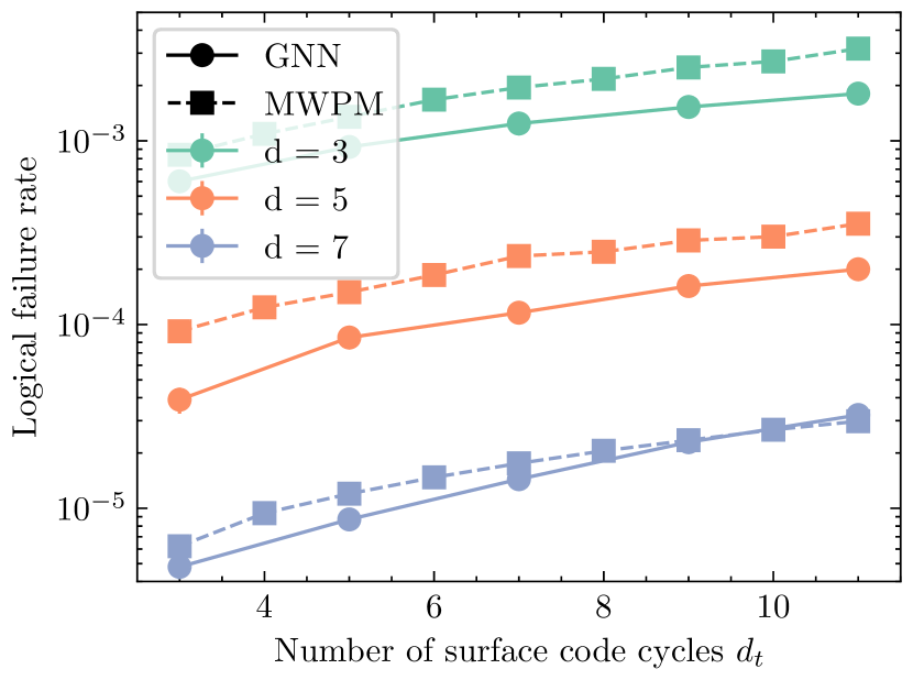
Figure 3: Decoding simulated experimental data Gidney (2021), with circuit-level noise, on the rotated surface code with code distance $d$. Logical failure rate versus number of rounds of stabilizer measurements $d_{t}$. Comparing GNN decoder trained on the detector data with MWPM decoder Higgott (2021) that has full information of the data-generating error model. Each data point is evaluated over $10^{8}$ samples ($10^{7}$ for $d<7$), memory-Z, at a reference error rate of $p=1\cdot 10^{-3}$.

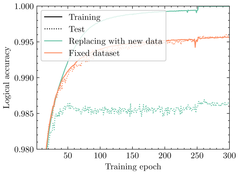
Figure 4: GNN training and test accuracy versus number of training epochs for circuit-level noise, comparing training using a fixed dataset to replacing 25% of the data after each epoch. We see that the latter setup is crucial to avoid overfitting, allowing the test accuracy to closely follow the training accuracy. Code distance $d=5$, with $d_{t}=5$ cycles, dataset size $5\cdot 10^{6}$ samples using an error rate randomly selected from $p=[0.001,0.002,...,0.005]$. The test set is a fixed dataset of the same type containing $5\cdot 10^{4}$ data points. (Sharp kink at 250 epochs correspond to a decrement of the learning rate.)

IV.2 Repetition code using experimental data

Having trained GNN based decoders on simulated experimental data in the previous section, we now turn to real experimental data. We use the public data provided together with Google Quantum AI (2023). This contains data on both the $d=3$ and $d=5$ surface codes as well as the $d=25$ bit-error correcting repetition code. All datasets are of the form described in II.3, thus readily transferred to the annotated and labeled graphs used to train the GNN, as described in III.1. The datasets contain approximately $10^{6}$ data points for the different codes, code distances, and varying number of stabilizer rounds.

Our attempts to train a GNN on the data provided for the various implementations of surface code were generally unsuccessful. While it gave good results on the training data, the logical failure rate on the test set was poor. Given the fact that on the order of $10^{9}$ data points were used for the simulated circuit-level noise on the surface code (IV.1), it is not surprising that the significantly smaller dataset turned out to be insufficient. The network cannot achieve high accuracy without overfitting to the training data given the relatively small dataset.

For the repetition code, the data which is provided is of a single type, for a $d=25$ code measured over $d_{t}=50$ rounds. Each round thus contains the measurement of 24 ancilla qubits for the $ZZ$ stabilizers of the two neighboring data qubits along a one-dimensional path. As done in Google Quantum AI (2023) this data can be split up into data for smaller repetition codes, by simply restricting to stabilizers over a subset of $d$ subsequent data qubits. In this way the dataset can be increased by a factor $25-(d-1)$, and used to train a single GNN for each code distance. It should be noted that this is suboptimal, compared to generating the same amount of data on single distance $d$ device, as variations in the performance of the constituent qubits and gates will be averaged out in the dataset. Nevertheless, using this scheme we successfully trained GNN decoders for short distance repetition codes, with test accuracies shown in Figure 5. Results for (what we refer to as) “Device-optimized MWPM” is taken from Google Quantum AI (2023). The GNN decoder performs almost on par with this sophisticated matching decoder for $d=3$. As expected, the relative performance deteriorates with increased code distance. We expect that we would need more training data for larger code distance, but instead we have access to less.

As the comparison with the matching decoder that uses a device specific error model may be biased compared to using training data from different devices, as mentioned above, we also give results for an “uniformed” matching decoder with edge weights based on the 1-norm distance between space-time coordinates. It may also be noted that using MWPM corresponds to a near optimal decoder for the repetition code, at least for the case of phenomenological measurement noise where it is equivalent to bit-flip error surface code. This is in contrast to the surface code, for which MWPM is suboptimal, even in the case of perfect stabilizers. Thus, outperforming MWPM for the repetition code may be more challenging than for the surface code.

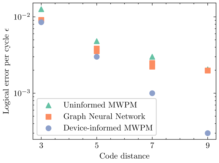
Figure 5: Decoding experimental data Google Quantum AI (2023) on the repetition code with code distance $d$, over 50 rounds of stabilizer measurements. Comparing GNN decoder, using a dataset containing $(26-d)\cdot 5\cdot 10^{7}$ graphs, with a MWPM decoder with “device-optimized” edge weights (Google Quantum AI (2023)) and a simple model-free MWPM decoder with 1-norm edge weights. The training-test split of the dataset is 99 to 1, and the logical failure rate is mapped to an error rate per round. Results for two different random training-test splits are shown.

Figure 6: Training curves for the GNN decoder on repetition code, following Figure 5. Each epoch trains through the whole training set, which eventually leads to overfitting, where the training accuracy starts to significantly surpass the test accuracy. To maximize the amount of training data, no validation set was used. No early stopping was implemented in order to avoid optimizing results to the test set.

IV.3 Surface code with perfect stabilizers

To complement the results on simulated and real experimental data we have also trained the GNN decoder on the surface code with perfect stabilizers under depolarizing noise. The same network (see Appendix A) is used as for circuit-level noise, but trained at $p=[0.01,0.05,0.1,0.15]$. Results up to code distance $d=15$ are shown in Figure 7 and found to significantly outperform MWPM. We also compare to a tensor network based Tuckett (2020) maximum likelihood decoder (MLD), showing that for code distance $d=5$ the GNN decoder has converged to the level of being an approximate MLD.

We do not attempt to derive any threshold for the GNN decoder. Given a sufficiently expressive network we expect that the decoder would eventually converge to a maximum likelihood decoder, but in practice the accuracy is limited by the training time. It gets progressively more difficult to converge the training for larger code distances, which means that any threshold estimate will be a function of the training time versus code distance. In fact, in principle, since the threshold is a $d\rightarrow\infty$ quantity, we would not expect that a supervised learning algorithm can give a proper threshold if trained separately for each code distance. Nevertheless, through GNN’s it is quite natural to use the same network to decode any distance code, as the data objects (detector graphs) have the same structure. We have investigated training the same network for different code distances and different number of rounds. This shows some promise, but so far does not achieve accuracy levels that can match MWPM.

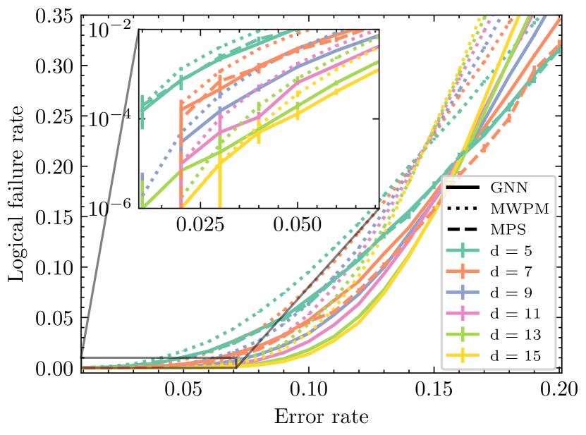
Figure 7: Decoding the rotated surface code with perfect stabilizers and code distance $d$. Logical failure rate versus error rate $p$, for depolarizing noise, evaluated over failures with respect to both $X_{L}(\lambda_{X})$ and $Z_{L}(\lambda_{Z})$. Comparing the GNN decoder with MWPM decoder that has full information of the data-generating error model. Each data point is evaluated over $10^{5}$ data points. Dashed lines is the accuracy using a matrix product state (MPS) decoder Tuckett (2020) at code distances 5 and 7, evaluated over $10^{4}$ data points.

IV.4 Scalability

We are limited to relatively small codes in this work. For the repetition code using experimental data, it is quite clear that main limitation to scaling up the code distance is the size of the available dataset. For the surface code using simulated data it is challenging to increase the code distance while still surpassing MWPM. As the logical failure rates decrease exponentially with code distance, the test accuracy of the supervised training needs to follow. One way to counter this is to increase the number of stabilizer cycles, $d_{t}$, but this also increases the graph size, making the training more challenging from the perspective of increased memory requirements as well as the increased complexity of the data.

Nevertheless, it is interesting to explore the intrinsic scalability of the algorithm, by quantifying how the decoding time using a fixed size GNN scales with the code size. Here we present results on the decoding time per syndrome for the surface code, as a function of code volume $d^{2}d_{t}$, at fixed error rate. The network architecture is the same as used for all the results in this paper, as described in Appendix A. In line with expectations, the GNN inference scales approximately linearly with the code volume, i.e. average graph size, $T\sim d^{2}d_{t}$ (with $d_{t}=1$ for perfect stabilizers). The number of matrix operations per graph convolutional layer, following Equation 3, is proportional to the number of nodes times the number of edges. The number of layers is fixed, multiplying this by a constant factor. The feature vector pooling is proportional to the number of nodes, whereas the subsequent dense network classifiers are independent of the graph size. We find that inference scales slightly better than the highly optimized matching decoder. However, several caveats are in order. 1) The size of the GNN is fixed. Larger code sizes may eventually require scaled up networks, unless the error rate is scaled down accordingly 2) The network has not been trained on code distances larger than $d=15$ (2D). It is only a test of the decoding time, not the accuracy. 3) For GNN inference, the data is batched in order to eliminate a fixed loading time to the GPU. Treating batched data doesn’t seem viable for real time decoding. Similarly our graph construction algorithm is slower, scaling quadratically with code volume, and this time has also been removed to get decoding time per graph. These are both issues that most likely can be improved significantly with more hardware efficient algorithms, and, in the longer term, special purpose hardware.

V Conclusion and Outlook

In this paper we develop a model-free, data-driven, approach to decoding quantum error correcting stabilizer codes, using graph neural networks. A real or simulated memory experiment is represented as a single detector graph, with annotated nodes corresponding to the type of stabilizer and its space-time coordinate, and labeled by the measured logical operation on the encoded qubit. The maximal node degree is capped by cropping edges between distant nodes. The data is used to train a convolutional GNN for graph classification, with classes corresponding to logical Pauli operations, and used for decoding. We show that we can use real and simulated experimental data,for the repetition code and surface code respectively, to train a decoder with logical failure rates on par with minimum weight perfect matching, despite the latter having detailed information about the underlying real or simulated error channels. The use of a graph structure provides an efficient way to store and process the syndrome data. To train the GNN requires significant amounts of training data, but as shown in the case of simulated experiments, data can be produced in parallel with training. Network inference, i.e., using the network as a decoder, is fast, scaling approximately linearly with the space-time dimension of the code.

As an extension of this work there are several interesting possibilities to explore. One example is to use a GNN for edge weight generation within a hybrid algorithm with a matching decoder (similarly to Chen et al. (2021)). This would depart from the pure data-driven approach pursued in this paper, with peak performance limited by the matching decoder, but with the potential advantage of requiring less data to train. An alternative to this, to potentially improve performance and lower data requirements, is to use device specific input into edge weights, or encode soft information on measurement fidelities into edge or node features.

Going beyond the most standard codes considered in this paper, we expect that any error correcting code for which labeled detector data can be generated can also be decoded with a GNN. This includes Clifford-deformed stabilizer codes Tuckett et al. (2018); Bonilla Ataides et al. (2021); Dua et al. (2022); Tiurev et al. (2022); Huang et al. (2022), color codes Bombin and Martin-Delgado (2006); Bombín (2015) or hexagonal stabilizer codes Wootton (2015, 2021); Srivastava et al. (2022); Hetényi and Wootton (2023), where syndrome defects are not created in pairs, but potentially also Floquet type codes Haah and Hastings (2021); Kesselring et al. (2022). In addition, heterogeneous and correlated noise models deMarti iOlius et al. (2022); Tiurev et al. (2023) would also be interesting to explore, where in particular the latter is difficult to handle with most standard decoders.

The software code for the project can be found at git .

Appendix A GNN architecture and training

Figure 9 displays the architecture of the GNN decoder. The node features are sent through 7 subsequent graph convolutional layers (Equation 3). The node features are passed through a rectified linear unit (ReLU) activation function (which corresponds to chopping negative values) after each layer. After the graph convolutional layers, the node features from all nodes are pooled into one high-dimensional vector by computing the mean across all nodes. This vector is then cloned and sent to two identical fully connected neural networks. Both heads consist of 4 dense layers which map the pooled node feature vector down to one real-valued number which is output in the range 0 to 1 through a sigmoid function. The input and output dimension $d_{in}$ and $d_{out}$ of the graph convolutional and dense layers can be found in Table 1.

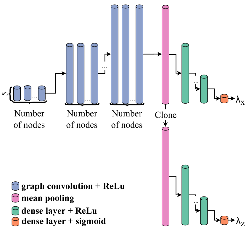
Figure 9: Schematic of the GNN architecture, with details in Table 1. The same architecture is used for all the results, except that for the repetition code there is only one output head. Also the input dimension is two (2D space-time coordinate) for the repetition code and four (two types of stabilizers, and 2D spatial coordinate) for the surface code with perfect stabilizers.

Layer	$d_{in}$	$d_{out}$
GraphConv1	5	32
GraphConv2	32	128
GraphConv3	128	256
GraphConv4	256	512
GraphConv5	512	512
GraphConv6	512	256
GraphConv7	256	256
Dense1 X	256	128
Dense2 X	128	181
Dense3 X	128	32
Dense4 X	32	1
Dense1 Z	256	128
Dense2 Z	128	181
Dense3 Z	128	32
Dense4 Z	32	1

Table 1: Overview over the input and output dimension of the graph convolutional and dense layers of the GNN decoder.

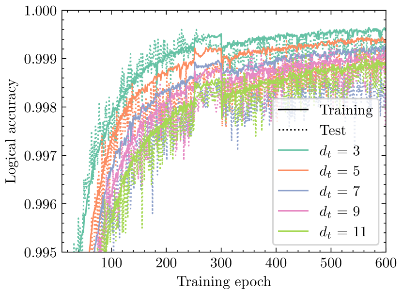
Figure 10: Example of training and validation accuracy versus the number of epochs of training for code distance 5. One epoch corresponds to training with a dataset containing $5\cdot 10^{6}$ detector graphs of different error rates, as in Figure 4. The test set is a fixed dataset of the same type containing $5\cdot 10^{4}$ data points. After each epoch the oldest 25% of the dataset is replaced with new data to avoid overfitting to the training data. Kink at 300 epochs correspond to decrement of the learning rate, whereas the spikes are due to network fluctuations.

Networks are trained on NVIDIA Tesla A100 HGX GPU’s using the python multiprocessing module to generate data in parallel on a CPU. For gradient descent, samples are batched in batches of size $10^{3}$. The learning rate is set to $10^{-4}$ and decreased manually to $10^{-5}$, whenever the validation accuracy reached a plateau. An example of a training history for $d=5$ and varying number of surface code cycles $d_{t}$ is shown in Figure 10. For this example, with $d_{t}=5$, 100 epochs of training takes approximately 10 hours. The code is available at git .

Appendix B Stabilizer circuits and error model for circuit-level noise

Quantum circuits for weight-four $Z$- ($X$-) stabilizers of the surface code are displayed in Figure 11 (12). The gate set used for the stabilizer measurements consists of the Hadamard gate $(H)$, and the $CNOT$ gate. Under circuit-level noise, single-qubit depolarizing noise gate $D_{p}$ (which applies gate $\sigma_{i},i\in\{X,Y,Z\}$ where any of the gates is applied with probability $p/3$, and $I$ with probability $1-p$) acts on the data qubits before each stabilizer measurement cycle and on each target qubit after single-qubit gates. Two-qubit depolarizing noise gates (which apply gate $\sigma_{i}\sigma_{j},i,j\in\{I,X,Y,Z\}$, where $II$ is acted on with probability $1-p$, and the rest with probability $p/15$) act on the two qubits involved after every two-qubit gate. Furthermore, each qubit suffers from reset- and measurement-error with probability $p$, displayed by operators $X_{p}$ when measuring and resetting in the computational basis.

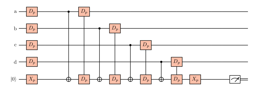
Figure 11: Quantum circuit for measuring the weight-four stabilizer $Z_{\text{abcd}}$ under circuit-level noise.

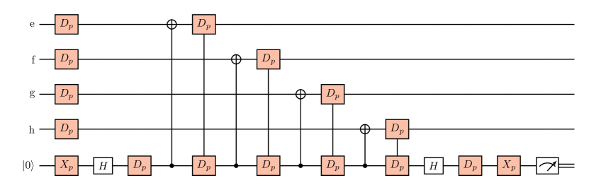
Figure 12: Quantum circuit for measuring the weight-four stabilizer $X_{\text{efgh}}$ under circuit-level noise.

References

- Shor (1995) Peter W. Shor, “Scheme for reducing decoherence in quantum computer memory,” Physical Review A 52, R2493–R2496 (1995).
- Steane (1996) A. M. Steane, “Error Correcting Codes in Quantum Theory,” Physical Review Letters 77, 793–797 (1996).
- Gottesman (1997) Daniel Gottesman, “Stabilizer Codes and Quantum Error Correction,” (1997), arXiv:quant-ph/9705052 .
- Terhal (2015) Barbara M. Terhal, “Quantum error correction for quantum memories,” Reviews of Modern Physics 87, 307–346 (2015).
- Girvin (2021) Steven M. Girvin, “Introduction to quantum error correction and fault tolerance,” (2021), arXiv:2111.08894 .
- Kim et al. (2023) Youngseok Kim, Andrew Eddins, Sajant Anand, Ken Xuan Wei, Ewout van den Berg, Sami Rosenblatt, Hasan Nayfeh, Yantao Wu, Michael Zaletel, Kristan Temme, and Abhinav Kandala, “Evidence for the utility of quantum computing before fault tolerance,” Nature 618, 500–505 (2023).
- Temme et al. (2017) Kristan Temme, Sergey Bravyi, and Jay M Gambetta, “Error mitigation for short-depth quantum circuits,” Physical review letters 119, 180509 (2017).
- Li and Benjamin (2017) Ying Li and Simon C Benjamin, “Efficient variational quantum simulator incorporating active error minimization,” Physical Review X 7, 021050 (2017).
- Bravyi and Kitaev (1998) S. B. Bravyi and A. Yu. Kitaev, “Quantum codes on a lattice with boundary,” (1998), arXiv:quant-ph/9811052 .
- Dennis et al. (2002a) Eric Dennis, Alexei Kitaev, Andrew Landahl, and John Preskill, “Topological quantum memory,” Journal of Mathematical Physics 43, 4452–4505 (2002a).
- Kitaev (2003) A.Yu. Kitaev, “Fault-tolerant quantum computation by anyons,” Annals of Physics 303, 2–30 (2003).
- Raussendorf and Harrington (2007) Robert Raussendorf and Jim Harrington, “Fault-Tolerant Quantum Computation with High Threshold in Two Dimensions,” Physical Review Letters 98, 190504 (2007).
- Fowler et al. (2012) Austin G. Fowler, Matteo Mariantoni, John M. Martinis, and Andrew N. Cleland, “Surface codes: Towards practical large-scale quantum computation,” Physical Review A 86, 032324 (2012).
- Kelly et al. (2015) J. Kelly, R. Barends, A. G. Fowler, A. Megrant, E. Jeffrey, T. C. White, D. Sank, J. Y. Mutus, B. Campbell, Yu Chen, Z. Chen, B. Chiaro, A. Dunsworth, I.-C. Hoi, C. Neill, P. J. J. O’Malley, C. Quintana, P. Roushan, A. Vainsencher, J. Wenner, A. N. Cleland, and John M. Martinis, “State preservation by repetitive error detection in a superconducting quantum circuit,” Nature 519, 66–69 (2015).
- Takita et al. (2017) Maika Takita, Andrew W. Cross, A. D. Córcoles, Jerry M. Chow, and Jay M. Gambetta, “Experimental Demonstration of Fault-Tolerant State Preparation with Superconducting Qubits,” Physical Review Letters 119, 180501 (2017).
- Wootton and Loss (2018) James R. Wootton and Daniel Loss, “Repetition code of 15 qubits,” Phys. Rev. A 97, 052313 (2018).
- Wootton (2020) James R Wootton, “Benchmarking near-term devices with quantum error correction,” Quantum Science and Technology 5, 044004 (2020).
- Andersen et al. (2020) Christian Kraglund Andersen, Ants Remm, Stefania Lazar, Sebastian Krinner, Nathan Lacroix, Graham J. Norris, Mihai Gabureac, Christopher Eichler, and Andreas Wallraff, “Repeated quantum error detection in a surface code,” Nature Physics 16, 875–880 (2020).
- Satzinger et al. (2021) K. J. Satzinger et al., “Realizing topologically ordered states on a quantum processor,” Science 374, 1237 (2021).
- Egan et al. (2021) Laird Egan, Dripto M. Debroy, Crystal Noel, Andrew Risinger, Daiwei Zhu, Debopriyo Biswas, Michael Newman, Muyuan Li, Kenneth R. Brown, Marko Cetina, and Christopher Monroe, “Fault-tolerant control of an error-corrected qubit,” Nature 598, 281–286 (2021).
- Chen et al. (2021) Zijun Chen et al., “Exponential suppression of bit or phase errors with cyclic error correction,” Nature 595, 383–387 (2021).
- Erhard et al. (2021) Alexander Erhard, Hendrik Poulsen Nautrup, Michael Meth, Lukas Postler, Roman Stricker, Martin Stadler, Vlad Negnevitsky, Martin Ringbauer, Philipp Schindler, Hans J. Briegel, Rainer Blatt, Nicolai Friis, and Thomas Monz, “Entangling logical qubits with lattice surgery,” Nature 589, 220–224 (2021).
- Ryan-Anderson et al. (2021) C. Ryan-Anderson, J. G. Bohnet, K. Lee, D. Gresh, A. Hankin, J. P. Gaebler, D. Francois, A. Chernoguzov, D. Lucchetti, N. C. Brown, T. M. Gatterman, S. K. Halit, K. Gilmore, J. A. Gerber, B. Neyenhuis, D. Hayes, and R. P. Stutz, “Realization of real-time fault-tolerant quantum error correction,” Phys. Rev. X 11, 041058 (2021).
- Marques et al. (2021) J. F. Marques, B. M. Varbanov, M. S. Moreira, H. Ali, N. Muthusubramanian, C. Zachariadis, F. Battistel, M. Beekman, N. Haider, W. Vlothuizen, A. Bruno, B. M. Terhal, and L. DiCarlo, “Logical-qubit operations in an error-detecting surface code,” Nature Physics 18, 80–86 (2021).
- Postler et al. (2022) Lukas Postler, Sascha Heussen, Ivan Pogorelov, Manuel Rispler, Thomas Feldker, Michael Meth, Christian D. Marciniak, Roman Stricker, Martin Ringbauer, Rainer Blatt, Philipp Schindler, Markus Müller, and Thomas Monz, “Demonstration of fault-tolerant universal quantum gate operations,” Nature 605, 675–680 (2022).
- Krinner et al. (2022) Sebastian Krinner, Nathan Lacroix, Ants Remm, Agustin Di Paolo, Elie Genois, Catherine Leroux, Christoph Hellings, Stefania Lazar, Christian Kraglund Andersen, et al., “Realizing repeated quantum error correction in a distance-three surface code,” Nature 605, 669–674 (2022).
- Bluvstein et al. (2022) Dolev Bluvstein, Harry Levine, Giulia Semeghini, Tout T. Wang, Sepehr Ebadi, Marcin Kalinowski, Alexander Keesling, Nishad Maskara, Hannes Pichler, Markus Greiner, Vladan Vuletić, and Mikhail D. Lukin, “A quantum processor based on coherent transport of entangled atom arrays,” Nature 604, 451–456 (2022).
- Google Quantum AI (2023) Google Quantum AI, “Suppressing quantum errors by scaling a surface code logical qubit,” Nature 614, 676–681 (2023).
- Moses et al. (2023) S. A. Moses, C. H. Baldwin, M. S. Allman, R. Ancona, L. Ascarrunz, C. Barnes, J. Bartolotta, B. Bjork, P. Blanchard, M. Bohn, J. G. Bohnet, N. C. Brown, N. Q. Burdick, W. C. Burton, S. L. Campbell, J. P. Campora III au2, C. Carron, J. Chambers, J. W. Chan, Y. H. Chen, A. Chernoguzov, E. Chertkov, J. Colina, J. P. Curtis, R. Daniel, M. DeCross, D. Deen, C. Delaney, J. M. Dreiling, C. T. Ertsgaard, J. Esposito, B. Estey, M. Fabrikant, C. Figgatt, C. Foltz, M. Foss-Feig, D. Francois, J. P. Gaebler, T. M. Gatterman, C. N. Gilbreth, J. Giles, E. Glynn, A. Hall, A. M. Hankin, A. Hansen, D. Hayes, B. Higashi, I. M. Hoffman, B. Horning, J. J. Hout, R. Jacobs, J. Johansen, L. Jones, J. Karcz, T. Klein, P. Lauria, P. Lee, D. Liefer, C. Lytle, S. T. Lu, D. Lucchetti, A. Malm, M. Matheny, B. Mathewson, K. Mayer, D. B. Miller, M. Mills, B. Neyenhuis, L. Nugent, S. Olson, J. Parks, G. N. Price, Z. Price, M. Pugh, A. Ransford, A. P. Reed, C. Roman, M. Rowe, C. Ryan-Anderson, S. Sanders, J. Sedlacek, P. Shevchuk, P. Siegfried, T. Skripka, B. Spaun, R. T. Sprenkle, R. P. Stutz, M. Swallows, R. I. Tobey, A. Tran, T. Tran, E. Vogt, C. Volin, J. Walker, A. M. Zolot, and J. M. Pino, “A race track trapped-ion quantum processor,” (2023), arXiv:2305.03828 [quant-ph] .
- Sundaresan et al. (2023) Neereja Sundaresan, Theodore J Yoder, Youngseok Kim, Muyuan Li, Edward H Chen, Grace Harper, Ted Thorbeck, Andrew W Cross, Antonio D Córcoles, and Maika Takita, “Demonstrating multi-round subsystem quantum error correction using matching and maximum likelihood decoders,” Nature Communications 14, 2852 (2023).
- Gidney (2021) Craig Gidney, “Stim: a fast stabilizer circuit simulator,” Quantum 5, 497 (2021).
- Higgott (2021) Oscar Higgott, “Pymatching: A python package for decoding quantum codes with minimum-weight perfect matching,” arXiv preprint arXiv:2105.13082 (2021).
- Knill (2005) Emanuel Knill, “Quantum computing with realistically noisy devices,” Nature 434, 39–44 (2005).
- de Beaudrap and Horsman (2020) Niel de Beaudrap and Dominic Horsman, “The ZX calculus is a language for surface code lattice surgery,” Quantum 4, 218 (2020).
- Wootton and Loss (2012) James R. Wootton and Daniel Loss, “High Threshold Error Correction for the Surface Code,” Physical Review Letters 109, 160503 (2012).
- Hutter et al. (2014) Adrian Hutter, James R. Wootton, and Daniel Loss, “Efficient Markov chain Monte Carlo algorithm for the surface code,” Physical Review A 89, 022326 (2014).
- Bravyi et al. (2014) Sergey Bravyi, Martin Suchara, and Alexander Vargo, “Efficient algorithms for maximum likelihood decoding in the surface code,” Physical Review A 90, 032326 (2014).
- Hammar et al. (2022) Karl Hammar, Alexei Orekhov, Patrik Wallin Hybelius, Anna Katariina Wisakanto, Basudha Srivastava, Anton Frisk Kockum, and Mats Granath, “Error-rate-agnostic decoding of topological stabilizer codes,” Phys. Rev. A 105, 042616 (2022).
- Pryadko (2020) Leonid P Pryadko, “On maximum-likelihood decoding with circuit-level errors,” Quantum 4, 304 (2020).
- Chubb (2021) Christopher T. Chubb, “General tensor network decoding of 2d pauli codes,” (2021).
- Edmonds (1965) Jack Edmonds, “Paths, trees, and flowers,” Canadian Journal of Mathematics 17, 449 (1965).
- Dennis et al. (2002b) Eric Dennis, Alexei Kitaev, Andrew Landahl, and John Preskill, “Topological quantum memory,” Journal of Mathematical Physics 43, 4452 (2002b).
- Wang et al. (2010) D. S. Wang, A. G. Fowler, A. M. Stephens, and L. C. L. Hollenberg, “Threshold Error Rates for the Toric and Planar Codes,” Quantum Information & Computation 10, 456 (2010).
- Wang et al. (2011) David S. Wang, Austin G. Fowler, and Lloyd C. L. Hollenberg, “Surface code quantum computing with error rates over 1%,” Physical Review A 83, 020302 (2011).
- Fowler (2015) Austin G Fowler, “Minimum weight perfect matching of fault-tolerant topological quantum error correction in average O(1) parallel time,” Quantum Information and Computation 15, 145 (2015).
- Brown (2022) Benjamin J. Brown, “Conservation laws and quantum error correction: towards a generalised matching decoder,” (2022).
- Delfosse (2014) Nicolas Delfosse, “Decoding color codes by projection onto surface codes,” Physical Review A 89 (2014), 10.1103/physreva.89.012317.
- Stephens (2014) Ashley M. Stephens, “Efficient fault-tolerant decoding of topological color codes,” (2014).
- Delfosse and Nickerson (2021) Nicolas Delfosse and Naomi H. Nickerson, “Almost-linear time decoding algorithm for topological codes,” Quantum 5, 595 (2021).
- Tuckett et al. (2020) David K. Tuckett, Stephen D. Bartlett, Steven T. Flammia, and Benjamin J. Brown, “Fault-tolerant thresholds for the surface code in excess of 5% under biased noise,” Physical Review Letters 124 (2020), 10.1103/physrevlett.124.130501.
- Sahay and Brown (2022) Kaavya Sahay and Benjamin J. Brown, “Decoder for the triangular color code by matching on a möbius strip,” PRX Quantum 3 (2022), 10.1103/prxquantum.3.010310.
- Berent et al. (2023) Lucas Berent, Lukas Burgholzer, Peter-Jan H. S. Derks, Jens Eisert, and Robert Wille, “Decoding quantum color codes with maxsat,” (2023).
- Benhemou et al. (2023) Asmae Benhemou, Kaavya Sahay, Lingling Lao, and Benjamin J. Brown, “Minimising surface-code failures using a color-code decoder,” (2023).
- Delfosse and Tillich (2014) Nicolas Delfosse and Jean-Pierre Tillich, “A decoding algorithm for CSS codes using the X/Z correlations,” in 2014 IEEE International Symposium on Information Theory (IEEE, 2014) pp. 1071–1075.
- Criger and Ashraf (2018) Ben Criger and Imran Ashraf, “Multi-path summation for decoding 2D topological codes,” Quantum 2, 102 (2018).
- Higgott et al. (2022) Oscar Higgott, Thomas C. Bohdanowicz, Aleksander Kubica, Steven T. Flammia, and Earl T. Campbell, “Fragile boundaries of tailored surface codes and improved decoding of circuit-level noise,” (2022).
- Caune et al. (2023) Laura Caune, Joan Camps, Brendan Reid, and Earl Campbell, “Belief propagation as a partial decoder,” (2023).
- Herold et al. (2015) Michael Herold, Earl T Campbell, Jens Eisert, and Michael J Kastoryano, “Cellular-automaton decoders for topological quantum memories,” npj Quantum Information 1, 15010 (2015).
- Kubica and Preskill (2019) Aleksander Kubica and John Preskill, “Cellular-Automaton Decoders with Provable Thresholds for Topological Codes,” Physical Review Letters 123, 020501 (2019).
- Miguel et al. (2023) Jonathan F. San Miguel, Dominic J. Williamson, and Benjamin J. Brown, “A cellular automaton decoder for a noise-bias tailored color code,” Quantum 7, 940 (2023).
- Duclos-Cianci and Poulin (2010) Guillaume Duclos-Cianci and David Poulin, “Fast Decoders for Topological Quantum Codes,” Physical Review Letters 104, 050504 (2010).
- Huang et al. (2020) Shilin Huang, Michael Newman, and Kenneth R. Brown, “Fault-tolerant weighted union-find decoding on the toric code,” Physical Review A 102, 012419 (2020).
- Torlai and Melko (2017) Giacomo Torlai and Roger G. Melko, “Neural Decoder for Topological Codes,” Physical Review Letters 119, 030501 (2017).
- Krastanov and Jiang (2017) Stefan Krastanov and Liang Jiang, “Deep neural network probabilistic decoder for stabilizer codes,” Scientific Reports 7, 11003 (2017).
- Varsamopoulos et al. (2017) Savvas Varsamopoulos, Ben Criger, and Koen Bertels, “Decoding small surface codes with feedforward neural networks,” Quantum Science and Technology 3, 015004 (2017).
- Baireuther et al. (2018) Paul Baireuther, Thomas E O’Brien, Brian Tarasinski, and Carlo WJ Beenakker, “Machine-learning-assisted correction of correlated qubit errors in a topological code,” Quantum 2, 48 (2018).
- Breuckmann and Ni (2018) Nikolas P Breuckmann and Xiaotong Ni, “Scalable Neural Network Decoders for Higher Dimensional Quantum Codes,” Quantum 2, 68 (2018).
- Baireuther et al. (2019) P Baireuther, M D Caio, B Criger, C W J Beenakker, and T E O’Brien, “Neural network decoder for topological color codes with circuit level noise,” New Journal of Physics 21, 013003 (2019).
- Chamberland and Ronagh (2018) Christopher Chamberland and Pooya Ronagh, “Deep neural decoders for near term fault-tolerant experiments,” Quantum Science and Technology 3, 044002 (2018).
- Nautrup et al. (2019) Hendrik Poulsen Nautrup, Nicolas Delfosse, Vedran Dunjko, Hans J Briegel, and Nicolai Friis, “Optimizing Quantum Error Correction Codes with Reinforcement Learning,” Quantum 3, 215 (2019).
- Maskara et al. (2019) Nishad Maskara, Aleksander Kubica, and Tomas Jochym-O’Connor, “Advantages of versatile neural-network decoding for topological codes,” Physical Review A 99, 052351 (2019).
- Ni (2020) Xiaotong Ni, “Neural Network Decoders for Large-Distance 2D Toric Codes,” Quantum 4, 310 (2020).
- Sweke et al. (2020) Ryan Sweke, Markus S Kesselring, Evert PL van Nieuwenburg, and Jens Eisert, “Reinforcement learning decoders for fault-tolerant quantum computation,” Machine Learning: Science and Technology 2, 025005 (2020).
- Andreasson et al. (2019) Philip Andreasson, Joel Johansson, Simon Liljestrand, and Mats Granath, “Quantum error correction for the toric code using deep reinforcement learning,” Quantum 3, 183 (2019).
- Colomer et al. (2020) Laia Domingo Colomer, Michalis Skotiniotis, and Ramon Muñoz-Tapia, “Reinforcement learning for optimal error correction of toric codes,” Physics Letters A 384, 126353 (2020).
- Fitzek et al. (2020) David Fitzek, Mattias Eliasson, Anton Frisk Kockum, and Mats Granath, “Deep Q-learning decoder for depolarizing noise on the toric code,” Physical Review Research 2, 023230 (2020).
- Gicev et al. (2021) Spiro Gicev, Lloyd CL Hollenberg, and Muhammad Usman, “A scalable and fast artificial neural network syndrome decoder for surface codes,” (2021), arXiv:2110.05854 .
- Bhoumik et al. (2021) Debasmita Bhoumik, Pinaki Sen, Ritajit Majumdar, Susmita Sur-Kolay, Latesh Kumar K J, and Sundaraja Sitharama Iyengar, “Efficient decoding of surface code syndromes for error correction in quantum computing,” (2021), arXiv:2110.10896 [quant-ph] .
- Théveniaut and van Nieuwenburg (2021) Hugo Théveniaut and Evert van Nieuwenburg, “A NEAT Quantum Error Decoder,” SciPost Physics 11, 5 (2021).
- Meinerz et al. (2022) Kai Meinerz, Chae-Yeun Park, and Simon Trebst, “Scalable neural decoder for topological surface codes,” Physical Review Letters 128 (2022), 10.1103/physrevlett.128.080505.
- Overwater et al. (2022) Ramon W. J. Overwater, Masoud Babaie, and Fabio Sebastiano, “Neural-network decoders for quantum error correction using surface codes: A space exploration of the hardware cost-performance tradeoffs,” IEEE Transactions on Quantum Engineering 3, 1–19 (2022).
- Chamberland et al. (2022) Christopher Chamberland, Luis Goncalves, Prasahnt Sivarajah, Eric Peterson, and Sebastian Grimberg, “Techniques for combining fast local decoders with global decoders under circuit-level noise,” (2022), arXiv:2208.01178 [quant-ph] .
- Zhang et al. (2023) Mengyu Zhang, Xiangyu Ren, Guanglei Xi, Zhenxing Zhang, Qiaonian Yu, Fuming Liu, Hualiang Zhang, Shengyu Zhang, and Yi-Cong Zheng, “A scalable, fast and programmable neural decoder for fault-tolerant quantum computation using surface codes,” (2023), arXiv:2305.15767 [quant-ph] .
- Wagner et al. (2022) Thomas Wagner, Hermann Kampermann, Dagmar Bruß, and Martin Kliesch, “Pauli channels can be estimated from syndrome measurements in quantum error correction,” Quantum 6, 809 (2022).
- Chen et al. (2022) Edward H. Chen, Theodore J. Yoder, Youngseok Kim, Neereja Sundaresan, Srikanth Srinivasan, Muyuan Li, Antonio D. Córcoles, Andrew W. Cross, and Maika Takita, “Calibrated decoders for experimental quantum error correction,” Phys. Rev. Lett. 128, 110504 (2022).
- Wagner et al. (2023) Thomas Wagner, Hermann Kampermann, Dagmar Bruß, and Martin Kliesch, “Learning logical pauli noise in quantum error correction,” Phys. Rev. Lett. 130, 200601 (2023).
- Bombin and Martin-Delgado (2007) H. Bombin and M. A. Martin-Delgado, “Optimal resources for topological two-dimensional stabilizer codes: Comparative study,” Physical Review A 76, 012305 (2007).
- Tomita and Svore (2014) Yu Tomita and Krysta M. Svore, “Low-distance surface codes under realistic quantum noise,” Physical Review A 90, 062320 (2014).
- Tuckett et al. (2019) David K. Tuckett, Andrew S. Darmawan, Christopher T. Chubb, Sergey Bravyi, Stephen D. Bartlett, and Steven T. Flammia, “Tailoring Surface Codes for Highly Biased Noise,” Physical Review X 9, 041031 (2019).
- Kipf and Welling (2016) Thomas N Kipf and Max Welling, “Semi-supervised classification with graph convolutional networks,” arXiv preprint arXiv:1609.02907 (2016).
- Wu et al. (2020) Zonghan Wu, Shirui Pan, Fengwen Chen, Guodong Long, Chengqi Zhang, and S Yu Philip, “A comprehensive survey on graph neural networks,” IEEE transactions on neural networks and learning systems (2020).
- Dwivedi et al. (2020) Vijay Prakash Dwivedi, Chaitanya K Joshi, Thomas Laurent, Yoshua Bengio, and Xavier Bresson, “Benchmarking graph neural networks,” arXiv preprint arXiv:2003.00982 (2020).
- Morris et al. (2021) Christopher Morris, Martin Ritzert, Matthias Fey, William L. Hamilton, Jan Eric Lenssen, Gaurav Rattan, and Martin Grohe, “Weisfeiler and leman go neural: Higher-order graph neural networks,” (2021), arXiv:1810.02244 [cs.LG] .
- Fey and Lenssen (2019) Matthias Fey and Jan Eric Lenssen, “Fast graph representation learning with pytorch geometric,” (2019), arXiv:1903.02428 [cs.LG] .
- Veličković et al. (2017) Petar Veličković, Guillem Cucurull, Arantxa Casanova, Adriana Romero, Pietro Lio, and Yoshua Bengio, “Graph attention networks,” arXiv preprint arXiv:1710.10903 (2017).
- Lee et al. (2019) Junhyun Lee, Inyeop Lee, and Jaewoo Kang, “Self-attention graph pooling,” (2019), arXiv:1904.08082 [cs.LG] .
- Knyazev et al. (2019) Boris Knyazev, Graham W. Taylor, and Mohamed R. Amer, “Understanding attention and generalization in graph neural networks,” (2019), arXiv:1905.02850 [cs.LG] .
- Gao and Ji (2019) Hongyang Gao and Shuiwang Ji, “Graph u-nets,” (2019), arXiv:1905.05178 [cs.LG] .
- Cangea et al. (2018) Cătălina Cangea, Petar Veličković, Nikola Jovanović, Thomas Kipf, and Pietro Liò, “Towards sparse hierarchical graph classifiers,” (2018), arXiv:1811.01287 [stat.ML] .
- Tuckett (2020) David Kingsley Tuckett, Tailoring surface codes: Improvements in quantum error correction with biased noise, Ph.D. thesis, University of Sydney (2020), (qecsim: https://github.com/qecsim/qecsim).
- Tuckett et al. (2018) David K. Tuckett, Stephen D. Bartlett, and Steven T. Flammia, “Ultrahigh error threshold for surface codes with biased noise,” Physical Review Letters 120 (2018), 10.1103/physrevlett.120.050505.
- Bonilla Ataides et al. (2021) J. Pablo Bonilla Ataides, David K. Tuckett, Stephen D. Bartlett, Steven T. Flammia, and Benjamin J. Brown, “The XZZX surface code,” Nature Communications 12, 2172 (2021).
- Dua et al. (2022) Arpit Dua, Aleksander Kubica, Liang Jiang, Steven T. Flammia, and Michael J. Gullans, “Clifford-deformed surface codes,” (2022).
- Tiurev et al. (2022) Konstantin Tiurev, Peter-Jan H. S. Derks, Joschka Roffe, Jens Eisert, and Jan-Michael Reiner, “Correcting non-independent and non-identically distributed errors with surface codes,” (2022).
- Huang et al. (2022) Eric Huang, Arthur Pesah, Christopher T. Chubb, Michael Vasmer, and Arpit Dua, “Tailoring three-dimensional topological codes for biased noise,” (2022).
- Bombin and Martin-Delgado (2006) H. Bombin and M. A. Martin-Delgado, “Topological quantum distillation,” Physical Review Letters 97 (2006), 10.1103/physrevlett.97.180501.
- Bombín (2015) Héctor Bombín, “Gauge color codes: optimal transversal gates and gauge fixing in topological stabilizer codes,” New Journal of Physics 17, 083002 (2015).
- Wootton (2015) James R Wootton, “A family of stabilizer codes for anyons and majorana modes,” Journal of Physics A: Mathematical and Theoretical 48, 215302 (2015).
- Wootton (2021) James R. Wootton, “Hexagonal matching codes with 2-body measurements,” (2021), arXiv:2109.13308 .
- Srivastava et al. (2022) Basudha Srivastava, Anton Frisk Kockum, and Mats Granath, “The XYZ2 hexagonal stabilizer code,” Quantum 6, 698 (2022).
- Hetényi and Wootton (2023) Bence Hetényi and James R. Wootton, “Tailoring quantum error correction to spin qubits,” (2023).
- Haah and Hastings (2021) Jeongwan Haah and Matthew B. Hastings, “Boundaries for the Honeycomb Code,” (2021), arXiv:2110.09545 .
- Kesselring et al. (2022) Markus S. Kesselring, Julio C. Magdalena de la Fuente, Felix Thomsen, Jens Eisert, Stephen D. Bartlett, and Benjamin J. Brown, “Anyon condensation and the color code,” (2022).
- deMarti iOlius et al. (2022) Antonio deMarti iOlius, Josu Etxezarreta Martinez, Patricio Fuentes, Pedro M. Crespo, and Javier Garcia-Frias, “Performance of surface codes in realistic quantum hardware,” Physical Review A 106 (2022), 10.1103/physreva.106.062428.
- Tiurev et al. (2023) Konstantin Tiurev, Peter-Jan H. S. Derks, Joschka Roffe, Jens Eisert, and Jan-Michael Reiner, “Correcting non-independent and non-identically distributed errors with surface codes,” (2023), arXiv:2208.02191 [quant-ph] .
- (116) https://github.com/LangeMoritz/GNN_decoder .