Learning Difference Equations with Structured Grammatical Evolution for Postprandial Glycaemia Prediction

Abstract

People with diabetes must carefully monitor their blood glucose levels, especially after eating. Blood glucose regulation requires a proper combination of food intake and insulin boluses. Glucose prediction is vital to avoid dangerous post-meal complications in treating individuals with diabetes. Although traditional methods, such as artificial neural networks, have shown high accuracy rates, sometimes they are not suitable for developing personalised treatments by physicians due to their lack of interpretability. In this study, we propose a novel glucose prediction method emphasising interpretability: Interpretable Sparse Identification by Grammatical Evolution. Combined with a previous clustering stage, our approach provides finite difference equations to predict postprandial glucose levels up to two hours after meals. We divide the dataset into four-hour segments and perform clustering based on blood glucose values for the two-hour window before the meal. Prediction models are trained for each cluster for the two-hour windows after meals, allowing predictions in 15-minute steps, yielding up to eight predictions at different time horizons. Prediction safety was evaluated based on Parkes Error Grid regions. Our technique produces safe predictions through explainable expressions, avoiding zones D (0.2% average) and E (0%) and reducing predictions on zone C (6.2%). In addition, our proposal has slightly better accuracy than other techniques, including sparse identification of non-linear dynamics and artificial neural networks. The results demonstrate that our proposal provides interpretable solutions without sacrificing prediction accuracy, offering a promising approach to glucose prediction in diabetes management that balances accuracy, interpretability, and computational efficiency.

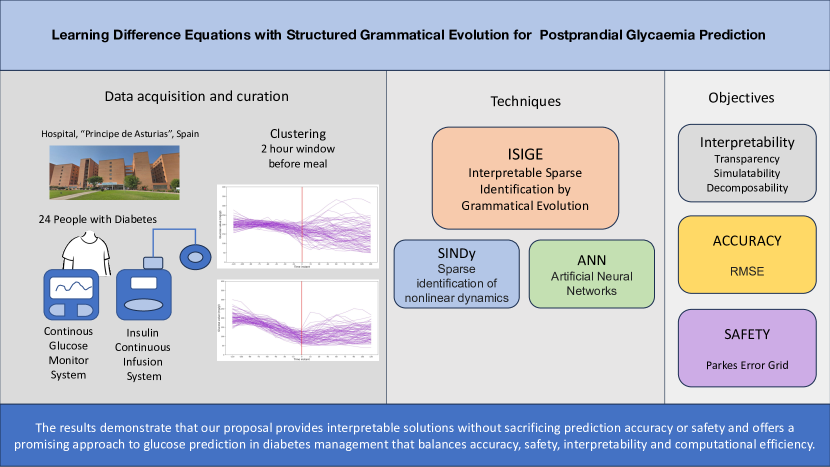
Figure 1: Graphical Abstract

This paper proposes a novel approach to glucose prediction in diabetes management that emphasises interpretability: Interpretable Sparse Identification by Grammatical Evolution (ISIGE)

The proposed technique combines clustering with ISIGE to obtain finite difference equations that predict postprandial glucose levels up to two hours after meals.

We have employed data from 24 different participants with diabetes mellitus type-I that was clustered based on blood glucose values for the two-hour window before the meal

Although ANN is one of the best-performing techniques for glucose prediction and one of the most commonly used methods in this field, in our study, both SINDy and ISIGE obtained better results in most clusters.

1 Introduction

More than 450 million people suffer from diabetes. There are two main types of diabetes: type I is an autoimmune disease that causes the destruction of insulin-producing cells (beta cells) of the pancreas, while type II appears when there is resistance to insulin action.

Insulin-dependent diabetes patients need to estimate, or even better to predict their blood glucose levels in the near term to manage their condition and prevent complications. Predicting glucose levels can help individuals make informed decisions about their diet, exercise, and especially the insulin and medication they use to maintain their blood glucose within a healthy range. The last decade has seen the rapid spread of new and reliable continuous glucose monitoring systems (CGM), which provide real-time glucose readings and trend data to help individuals adjust their treatment plan accordingly.

The availability of data from CGMs has lead the research in the field. Great efforts have been made in the search for accurate glucose prediction models. Some of them are black-box models [1], others are based on analytical models [2], and most of them provide predictions for a time horizon from 15 to 120 minutes [3]. Among them, symbolic regression (SR) [4] techniques and artificial neural networks (ANNs) obtained very good performance [5].

ANNs have become a popular tool for glucose prediction in the management of diabetes due to their ability to capture complex, non-linear relationships between input variables and glucose levels. However, one of the key challenges in using ANNs for glucose prediction is the lack of interpretability of the solutions they provide. ANNs can be viewed as black-box models, making it difficult to understand how they arrive at their predictions and limiting their usefulness in clinical decision making. This problem of interpretability has led researchers to explore alternative explainable AI techniques to provide both accurate forecasts and insight for clinicians.

This work aims to explore techniques for deriving finite difference equations that accurately represent the dynamics of blood glucose levels, with the benefit of obtaining interpretable models that can serve to aid the work not only of people with diabetes, but also of diabetes clinicians. To achieve this interpretability, we have developed a variant of grammatical evolution (GE) that produces sparse solutions: Interpretable Sparse Identification by Grammatical Evolution (ISIGE). This technique seeks to integrate the good results in the last years of Grammatical Evolution for blood glucose prediction,[6] and the advantages of a recently proposed method: sparse identification of non-linear dynamics (SINDy).

SINDy is an optimization-based method that constructs a sparse model of the dynamics of a system as a linear model with a set of non-linear base functions. To achieve sparsity, SINDy adds a sparsity-promoting regularization term which penalizes models with too many non-zero coefficients, forcing the algorithm to select a smaller subset of variables and interactions most relevant to the dynamics of the system. This helps to avoid overfitting, improve the interpretability of the model, and reduce computational complexity [7]. Conceptually, the approach is similar to fast function extraction (FFX) [8] but focuses on system dynamics.

In addition, to refine the models and predictions, we employ a clustering approach to group the glucose time series before meals which give us several scenarios for prediction. Due to the complexity of this situation and the need for a technique with good performance characteristics, we have implemented ISIGE using Dynamic Structured GE (DSGE). In addition, to reduce the risk of premature convergence and to improve the diversity of the generated solutions, we have applied the $\epsilon$-lexicase selection technique [9].

In this paper, we describe our technique and analyze the experimental results against SINDy and ANNs, in terms of precision, suitability for diabetes care and interpretability.

The results of this study are significant in several ways:

• The results demonstrate that the proposed ISIGE approach, together with SINDy, outperforms well tested ANNs in terms of prediction accuracy.

• ISIGE is the technique that provides the most accurate predictions. This is particularly important for glucose prediction in diabetes treatment, where accurate and safe predictions are crucial for clinical decision-making.

• The fact that ISIGE and SINDy show similar interpretability suggests that ISIGE can provide interpretable solutions without sacrificing prediction performance and safety.

These results offer a promising new approach to glucose prediction in diabetes management that balances accuracy, interpretability and computational efficiency.

The subsequent sections of this article are structured as follows: Section 2 presents an overview of the existing literature on utilizing machine learning (ML) techniques for hypoglycemia prediction. In Section 3, our approach is elucidated, encompassing the specific features of the grammar used in our version of DSGE, together with the iterative numerical evaluation algorithm used for the fitness computation. Section 4 outlines the workflow and primary techniques employed in this research as a point of reference. The experimental setup, data utilized, and the resulting outcomes obtained from our proposed approach are detailed in Section 5. Finally, Section 6 provides the concluding remarks of this study.

2 Related work

Dynamic models for glucose prediction are mathematical models that can simulate and predict behavior of blood glucose levels over time. They have been used in a variety of applications, such as personalized glucose control algorithms, prediction of hypoglycemia events, and optimization of insulin therapy.

There are three types of dynamic models for glucose prediction:

• Physiological models [2, 10, 11]: These models use a set of differential equations to simulate the dynamics of glucose and insulin in the body. Physiological models are based on our current understanding of the complex interactions between glucose and insulin in the body.

• Data-driven models [12, 13, 14, 15, 16, 17]: These are mathematical models that are constructed based on data obtained from individuals with diabetes. These models use statistical and machine learning techniques, to analyze the data and identify patterns that can be used to predict future glucose levels. Different models have been developed in conjunction with CGM systems to make short-term or long-term predictions.

• Hybrid models [18, 19, 20]: These models combine physiological and data-driven models to take advantage of the strengths of both types of models to improve the accuracy of glucose predictions.

As we can see, blood glucose prediction is a very active field of research, and although significant progress has been made, several challenges remain to be overcome, including:

• Individual differences: the metabolism of each person is unique, and blood glucose dynamics can vary significantly from individual to individual and from the situation of each person (e.g., changes during pregnancy, illness requiring medication administration, etc.).

• Delayed response: There is always a variable delayed response between insulin administration or carbohydrate intake and blood glucose value.

• Sensor limitations: The accuracy and reliability of glucose sensors can vary over their lifetime, so that the resulting noise can affect the data quality used for training and model prediction.

• Complex dynamics: Blood glucose dynamics are influenced by many factors that can interact in complex ways, such as food intake, physical activity, medication, sleep, and stress.

This paper addresses these challenges using two techniques that we consider particularly suitable for glucose prediction: structured grammatical evolution (SGE) and SINDy. These two approaches can handle large and complex datasets with noisy and incomplete data, automatically extract the most relevant inputs, and identify the main mathematical functions to describe glucose dynamics. Additionally, they generate interpretable models that provide the opportunity to be analyzed, allowing researchers better to understand the underlying dynamics of blood glucose regulation.

SINDy [21, 7] is a data-driven approach used to discover governing equations that describe the dynamics of a system. Although it is a relatively new approach several research papers have been published addressing problems on different fields including physics [22], network biology [23] or chemical kinetics [24].

The primary reference for GE applied to glucose forecasting is the book chapter from Hidalgo et al. [6], where a new approach for identifying mathematical models that can predict blood glucose levels in people with diabetes using GE is proposed. The approach was evaluated using data from the OhioT1DM dataset [25] containing glucose and physiological data from 43 people with diabetes. The results showed that the proposed system outperformed several baseline approaches regarding accuracy and interpretability, including linear regression, ARIMA models, and ANNs.

The lead article in the field of SGE is [26]. This paper presents a novel approach to predict glucose levels in people with diabetes using SGE, a variant of GE that encodes the chromosomes of individuals using a list of values corresponding to the productions of each non-terminal symbol to increase the locality of genetic operators. Different selection schemes can be used for SGE.

Spector [27] presented a preliminary report with a novel idea: lexicase selection. Lexicase selection has been applied to many optimisation problems. Helmuth et al. [28, 29] used lexicase selection to evolve models for several problems, being one of them predicting blood pressure based on a set of physiological features. LaCava and Spector (2016) [30], propose a variant (called Epsilon-lexicase) focused on continuous fitness landscapes that produces better results for symbolic regression problems. Spector et al. (2018) [31] used lexicase selection to evolve models for predicting protein-ligand binding affinity. The work from Stanton et al. [32] used lexicase selection to evolve robot controllers for tasks such as navigation and object manipulation.

3 Methods and techniques

A finite difference equation (FDE) is a mathematical expression that describes the difference between a variable $y$ at two discrete time points [33]. A FDE takes the form of Equation 1, where $\vec{x}$ represents a set of input variables involved in the equation, $y$ represents the target variable, and $\theta$ are optional calibration parameters.

$$\Delta y(t)=y(t+\Delta{t})-y(t)=f(\vec{x}(t),y(t),\theta)$$ (1)

FDEs are classified based on their properties, such as linearity, nonlinearity, and order, which is the highest difference in time steps that explicitly appear in the equation. For example, Equation 1 is a first-order equation, while Equation 2 is a second-order equation as it involves the difference between $y(t+2)$ and $y(t)$.

$$y(t+2\Delta{t})-y(t)=f(\vec{x}(t))$$ (2)

Variable	Description
$B_{I}$	Basal insulin
$I_{B}$	Insulin bolus.
$F_{\text{ch}}$	Carbohydrate intake.
HR	Heart rate
$G$	Glucose concentration.
$C$	Calories burned
$S$	Steps.

Table 1: Input variables in this study

Due to their simplicity, finite difference equations are handy for modelling dynamic processes which are measured with constant frequency (equidistant time steps), such as blood glucose levels measured by CGM. Equation 3, express the dynamics of glucose values as a finite difference equation problem. The description of the input variables is given in Table 1.

$$\Delta G(t)=G(t+\Delta_{t})-G(t)=f(G(t),B_{I}(t),I_{B}(t),F_{ch}(t),HR(t),C(t),S(t))$$ (3)

As is often the case in physical systems, we assume that in the glucose regulation system, only a few terms are relevant in defining its dynamics. Therefore, we can consider the governing equations are scattered in a high-dimensional non-linear function space. In this way, we aim to create a simplified model that accurately captures the essential dynamics of the system while minimising complexity. The SINDy algorithm is particularly suitable for this purpose. In subsection 3.1, we briefly explain how SINDy works. Then, in subsection 3.2, we present our proposal, ISIGE, which seeks to incorporate the benefits of SINDy within the paradigm of GE.

3.1 Sparse Identification of Nonlinear Dynamics (SINDy)

Algorithm 1 SINDy algorithm for Finite Difference Equations

1:procedure SINDy($\mathbf{X},\Delta(t),\lambda$)

2:     $\mathbf{X},\mathbf{\dot{X}}\leftarrow$ History States Variables

3:     $\mathbf{\Theta}(\mathbf{X})\leftarrow$ candidate nonlinear functions library matrix

4:     $\mathbf{\Theta}(\mathbf{x}^{T})\leftarrow$ vector of symbolic functions

5:     $\mathbf{x}^{P_{2}}\leftarrow$ quadratic non-linearities in the state x

6:     $\mathbf{\Theta}\lambda\leftarrow$ add regularization term to $\mathbf{\Theta}$ (LASSO)

7:     $\boldsymbol{\Xi}\leftarrow\boldsymbol{\xi}_{1},\boldsymbol{\xi}_{2},\boldsymbol{\xi}_{3},...$ sparse vectors of coefficients

8:     $\boldsymbol{\xi}k\leftarrow$ $\mathbf{\dot{X}}=\mathbf{\Theta}(\mathbf{X})\boldsymbol{\Xi}$, solve sparse regression

9:     Return $\mathbf{\dot{x}}_{k}=\mathbf{f}_{k}(\mathbf{x})=\mathbf{\Theta}(\mathbf{x}^{P_{2}})\boldsymbol{\xi}_{k}$

SINDy is a data-driven method for discovering the governing equations of a dynamical system from time series data [21, 7]. In Algorithm 1, we have summarized the main steps for SINDy.

• Data gathering (line 2): The first step is to collect data from the system that we want to model. The data are time-series measurements of the state variables of the system (Table 1).

• Construct a library of candidate functions (line 3): The next step is to construct a library of candidate functions that could potentially be part of the governing equations. In the general SINDy algorithm, these functions could include polynomials, trigonometric functions, exponentials, etc, depending on the system being modeled. In this work and based in our prior knowledge of the system, we have chosen up to $X^{P_{2}}$, quadratic non-linearities of $X$ (Equation 4).

  $$\textbf{$\Theta$}(X)=\left[\begin{array}[]{cccccccc}\vdots&\vdots&\vdots&\vdots&\\ 1&X&\vdots&X^{P_{2}}\\ \vdots&\vdots&\vdots&\vdots&\\ \end{array}\right]$$ (4)

• The development of all the linear combinations (line 5), are grouped in Equation 5, where $t_{0}$ represents the first time step, $t_{1}$ the subsequent time step, and so on.

  $$\textbf{$X^{P_{2}}$}=\left[\begin{array}[]{ccccc}G(t_{0})\cdot B_{I}(t_{0})&G(t_{0})\cdot I_{B}(t_{0})&G(t_{0})\cdot F_{C}H(t_{0})&\cdot\cdot\cdot&F_{C}H^{2}(t_{0})\\ G(t_{1})\cdot B_{I}(t_{1})&G(t_{1})\cdot I_{B}(t_{1})&G(t_{1})\cdot F_{C}H(t_{1})&\cdot\cdot\cdot&F_{C}H^{2}(t_{1})\\ \vdots&\vdots&\vdots&\vdots&\vdots\\ G(t_{n})\cdot B_{I}(t_{n})&G(t_{n})\cdot I_{B}(t_{n})&G(t_{n})\cdot F_{C}H(t_{n})&\cdot\cdot\cdot&F_{C}H^{2}(t_{n})\\ \end{array}\right]$$ (5)

• Add regularization (line 6): SINDy uses sequential threshold ridge regression as a regularization. The objective function $||\Theta\xi-\dot{X}_{t}||^{2}_{2}+\lambda||\xi||^{2}_{2}$ is minimized by iteratively performing least squares and masking out elements of the weight array $\xi$ that are below a given threshold $\lambda$. In this paper we used $\lambda=0.5$ which tests have shown to produce the best results.

• Solving the optimization problem (lines 7-8): through a sparse regression algorithm, we identify the combination of terms that best describes the observed dynamics of the system.

• Once the sparse coefficients have been found (line 9), we have the governing equations of the system.

3.2 Interpretable Sparse Identification by Grammatical Evolution

This study introduces a novel approach, ISIGE, to model blood glucose dynamics using FDEs. Specifically, we utilize DSGE, a variant of GE, to obtain $\hat{G}(t+\Delta(t))$ as expressed in equation 6 which comes from the expression 3.

$$\hat{G}(t+\Delta(t))=G(t)+\Delta G(t)=G(t)+f(\vec{x}(t))$$ (6)

One of the benefits of using DSGE is the ability to obtain explainable expressions, which enables us to analyze the impact and significance of different components in the system. Therefore, our proposed approach is expected to provide interpretable and efficient models for blood glucose dynamics. DSGE addresses two limitations of GE. First, it overcomes the low locality problem by ensuring that a slight change in the genotype results in a corresponding small change in the phenotype, thus ensuring high locality. Second, it eliminates redundancy, which occurs when different genotypes produce the same phenotype, by creating a one-to-one mapping between the genotype and the non-terminal. To achieve this, DSGE employs variable-size lists instead of the fixed-size lists used in GE.

3.2.1 $\epsilon$-Lexicase selection

The characteristics of our data are explained in depth in Section 4.3. Broadly speaking, we have grouped the data into clusters comprising multiple 4-hour glucose time series segments. The behaviour of these segments is highly varied (Figure 6), and if the selection mechanism of the evolutionary algorithm fails to take this into account, many individuals who do not achieve high fitness in all cases will be rejected. Because of this, we think of lexicase (and, more specifically, $\epsilon$-Lexicase) as a selection mechanism.

Lexicase selection [34] is a powerful search strategy used in evolutionary computation to overcome the problem of premature convergence. It works by selecting individuals that perform well in a randomly chosen subset of the fitness cases and repeating the process with the remaining fitness cases until only one individual is left. However, this method may become too selective, leading to limited search space exploration and the loss of diversity. To address this issue, $\epsilon$-Lexicase [9] selection was proposed, introducing a tolerance parameter, $\epsilon$. This parameter selects individuals that perform well within a certain threshold of the best-performing individuals in each subset. This approach allows for a more comprehensive search space exploration while preserving good individuals.

Algorithm 2 outlines the process of obtaining difference equations using ISIGE. We load the datasets and problem properties, then create an initial population and start the evolutionary process. We obtain the phenotypes (expressions) of each generation by decoding the population with the grammar. Using $\epsilon$-Lexicase selection, we determine the parents for the next population. We generate a new population by crossing and mutating the selected parents.

Algorithm 2 ISIGE

1:procedure  ISIGE($grammar,datasets,properties$)

2:     Load properties

3:     Load Datasets

4:     pop = Generate population(len_pop)

5:     for $i\leftarrow 0$ to ($N\_generations$ - 1) do

6:         for $j\leftarrow 0$ to ($len\_pop$ - 1) do

7:              $\hat{G}(t+\Delta{t})_{j}$ = decode(grammar, $pop_{j}$)          

8:         pop= $\epsilon$-Lexicase selection (datasets, pop , $f_{j}(\vec{x}(t)))$

9:         pop = Crossover(pop)

10:         pop = Mutation(pop)      

Where $\hat{G}(t+\Delta{t})_{j}$ comes from Equation 6

3.2.2 Iterative Numerical Evaluation

During the $\epsilon$-Lexicase selection process, we evaluate individuals from the current subpopulation using a specific dataset for each iteration. One difference in our approach is the application of an iterative numerical method to solve Equation 6. This equation calculates the glucose concentration for the next time step ($\hat{G}(t+\Delta t)$). We have developed algorithm 3, named Iterative Numerical Evaluation (INE), to implement this iterative numerical method. In our study, each time step ($t_{i}$) represents samples taken every 15 minutes within two hours after a meal. We evaluate the predicted glucose value at the next time step ($\hat{G}(t_{i+1})$) using various variables of the system ($\vec{x_{k}}(t_{i})$.) from the data set, in the case of glucose, only the first value is taken, and for the remaining iterations, the predicted value obtained in the previous step is used. Once predictions are made for all time instances, we calculate the Root Mean Square Error (RMSE) by comparing the predicted glucose values with the actual values using Equation 7. The resulting RMSE serves as the fitness measure for that individual on the specific dataset, indicating its performance for that dataset.

$$\text{RMSE}=\sqrt{\frac{1}{N}\sum_{t=1}^{N}\left(\hat{G}_{t}-G_{t}\right)^{2}}$$ (7)

In Equation 7, $N$ represents the total number of time instances, $\hat{G}_{t}$ denotes the predicted glucose value at time $t$, and $G_{t}$ represents the actual glucose value at time $t$.

The iterative numerical evaluation, algorithm 3, takes as input a function $f_{j}$ and a dataset $D_{k}$. It proceeds as follows:

1. Initialize the predicted glucose value at the starting time ($t_{0}$) as the actual glucose value from the dataset ($G_{k}(t_{0})$).

2. Iterate through each time step ($t_{i}$) from 0 to the total number of points in the dataset minus one.

3. Update the predicted glucose value at the next time step ($t_{i+1}$) by adding the function $f_{j}$ applied to the variables $\vec{x_{k}}(t_{i})$.

4. Calculate the fitness $F_{j}$ of individual $j$ for the dataset $k$ by comparing the predicted glucose values ($\hat{G}$) with the actual glucose values ($G_{k}$) using the Root Mean Square Error (RMSE) measure, equation 7.

5. Return the fitness $F_{j}$.

Algorithm 3 Iterative numerical evaluation

1:procedure Iterative_numerical_evaluation($f_{j}$,$D_{k}$)

2:     $\hat{G}(t_{0})=G_{k}(t_{0})$

3:     for $i\leftarrow 0$ to ($num\_points$ - 1) do

4:         $\hat{G}(t_{i+1})$ = $\hat{G}(t_{i})+f_{j}(\vec{x_{k}}(t_{i}))$      

5:     $F_{j}$=RMSE($\hat{G}$, $G_{k}$)

6:     return $F_{j}$

Where $G_{k}$ is the set of actual glucose values of $D_{k}$, $\hat{G}$ is the set of predicted values for the same points of $D_{k}$, $\vec{x_{k}}(t_{i})$ the set of variables of $D_{k}$ for time i and $F_{j}$ is the fitness of individual j for $D_{k}$.

This process is repeated for each individual in the subpopulation of this $\epsilon$-Lexicase selection iteration.

3.2.3 Grammar

Creating a grammar to define the search space is essential in DSGE. This involves establishing how to generate constants, which operations to use, which structures to generate expressions and which variables to incorporate. In Figure 2, we can see that the set of base functions used in the SINDy algorithm (subsection 3.1) is equivalent to the ISIGE grammar, but there is an important consideration here. Due to the method used to evaluate the numerical expressions, it is only possible to calculate the values of the variables for one time step at each iteration.

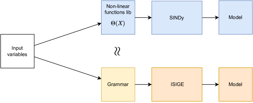
Figure 2: Common steps between SINDy and ISIGE, our proposal

In Figure 3, we present the grammar used in this work in Backus Naur Form (BNF), which is crucial for obtaining the desired FDEs. One of the essential elements of this grammar is the initial definition of the $<$func$>$ expression, which establishes that all expressions must follow the form G + $<$ expr$>$, ensuring that the resulting expressions are in the FDE form. Another critical element is the $<$var$>$ field, which includes individual variables (excluding G, which has already been included), first-order non-linearities, and second-order non-linearities. This approach allows us to mimic the set of base functions used in the SINDy algorithm. Using this grammar, we can effectively generate diverse FDEs that describe the system behaviour and make accurate predictions.

⬇

# Model expression

<func> ::= G + <expr>

<expr> ::= (<expr> <op> <expr>) | (<cte> <op> <var> <op> <expr>)

| <var> | (-<var>)

| pow(<var>,<sign><exponent>)

| (-pow(<var>,<sign><exponent>))

<var> ::= $B_{I}|I_{B}|F_{ch}|\text{HR}|C|S|$

# First order

$G\cdot B_{I}|G\cdot I_{B}|G\cdot F_{ch}|G\cdot\text{HR}|G\cdot C|G\cdot S|$

$B_{I}\cdot I_{B}|B_{I}\cdot F_{ch}|B_{I}\cdot\text{HR}|B_{I}\cdot C|B_{I}\cdot S|$

$I_{B}\cdot F_{ch}|I_{B}\cdot\text{HR}|I_{B}\cdot C|I_{B}\cdot S|$

$F_{ch}\cdot\text{HR}|F_{ch}\cdot C|F_{ch}\cdot S|$

$\text{HR}\cdot C|\text{HR}\cdot S|$

$C\cdot S|$

# Second order

$G\cdot G|B_{I}\cdot B_{I}|I_{B}\cdot I_{B}|F_{ch}\cdot F_{ch}|\text{HR}\cdot\text{HR}|C\cdot C|S\cdot S$

<op> ::= +|-|$\cdot$

<cte> ::= <base> $\cdot$ pow(10,<sign><exponent>)

<base> ::= 1|2|3|4| $\cdot\cdot\cdot$ |99

<exponent> ::= 1|2|3|4|5|6|8|9

<sign> ::= +|-

Figure 3: Grammars used for ISIGE in BNF.

4 Workflow

Figure 4 summarizes the workflow of the methodology applied in this work. It consists on several steps, further described in this section: data acquisition, data preprocessing, data partitioning, clustering, modelling, testing and results comparison.

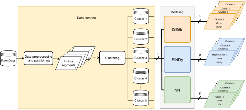
Figure 4: Workflow diagram of our methodology. The stages represented are: data acquisition, data preprocessing, data partitioning, clustering, modelling.

4.1 Data acquisition

For this study, we used data from 24 participants of the Hospital Universitario Príncipe de Asturias, Madrid, Spain. Two different devices were used to obtain the raw data: A continuous glucose monitor (CGM) system (Free Style Libre sensor) and an activity monitoring wristband (Fitbit Ionic). The CGM measures interstitial glucose levels every 15 minutes, while the wristband records data on calories, steps and heart rate at different time frequencies.

In addition, information about insulin and carbohydrate intakes was recorded by two different methods depending on the insulin administration mode. Participants wearing an automatic insulin continuous infusion system (insulin pumps) obtain this information directly from the device (Medtronic or Roche systems). Participants under multiple doses of insulin (MDI) therapy recorded the information about basal insulin, insulin boluses, and carbohydrate intakes using a mobile application.

The studies involving human participants were reviewed and approved by Hospital Universitario Príncipe de Asturias (Spain). The patients/participants provided their written informed consent to participate in this study.

4.2 Data Preprocessing

To use the recorded data for the modelling of the blood glucose level several preprocessing steps had to be performed. This includes both cleaning as well as feature engineering.

4.2.1 Features for the absorption of carbohydrates and insulin

Since the dissolution of substances in the body occurs gradually, we preprocessed both the reported insulin bolus and carbohydrate values using two functions to spread the uptake over multiple observations: the Berger function (Equation 8 and Figure 5(a)) [35] and the Bateman function (Equation 9 and Figure 5(b)) [36].

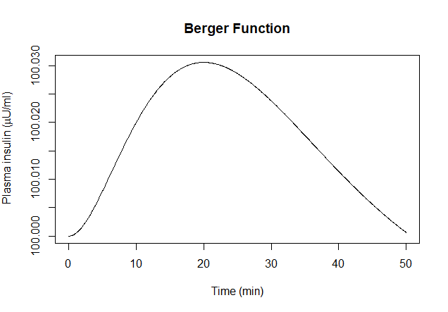
(a) Possible plasma insulin evolution based on Berger equation

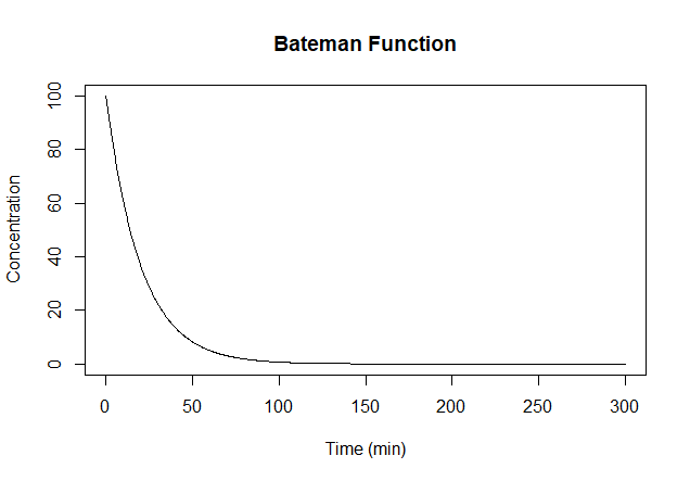
(b) Possible insulin concentration evolution based on Bateman Function

Figure 5: Representation of Berger and Bateman function

The Berger function is

$$\frac{dA}{dt}=\frac{s\cdot t^{s}\cdot{(a\cdot D\cdot b)}^{s}\cdot D}{t\cdot({(a\cdot D\cdot b)}^{s}+t^{s})^{2}}-A$$ (8)

where $A$ is the plasma insulin, $D$ the dose, $t$ the time after the consumption, $s$ the mean absorption rate and $a$ and $b$ are parameters to characterize dependency on $D$. We use the parameter values $s=1.6$, $a=5.2$ and $b=41$ [35].

The Bateman function is

$$c(t)=f\cdot\frac{D}{V}\cdot\frac{k_{a}}{k_{a}-k_{e}}\cdot(e^{-k_{a}\cdot t}-e^{-k_{e}\cdot t})$$ (9)

where $k_{a}$ is the absorption rate, $k_{e}$ the elimination rate, $D$ the dose, $t$ the time since consumption, $V$ the volume of distribution and $f$ the bioavailabilty. We used the parameter values $k_{a}=0.1$, $k_{e}=0.2$, $V=0.5$ and $f=0.5$ [36].

Both functions convert an instant input such as the insulin bolus as well as reported meals that the uptake of the substance into the body does not take place abruptly but is distributed over a longer period of time.

4.2.2 Time-Shifts

We added time-shifted features for the carbohydrates and the bolus values. The observations have a time shift of thirty minutes to the past, and the data points are recorded at fifteen-minute intervals.

4.2.3 Mean Values

Since the heart rate and steps measurements every 15 minutes can change quickly, we smoothed them using a moving average with a window size of 30 minutes (two observations).

4.2.4 Creation of Segments

We define a segment as the period of 2 hours before and after a reported meal (i.e. carbohydrate input). Segments may overlap if two meals are taken within a time span of two hours. For each of those segments we check for the following constraints:

1. Each of the parameter values for each time-step has to be greater than 0.

2. We only allow interpolated data up to one hour.

3. A change between time steps must not be more than 25% of the previous value.

4.3 Clustering

We used k-means clustering to cluster segments based on the 2-hour window of glucose measurements before the meal. We tried $k\in{3,5,7,9,11,13,15,17,19}$ and selected $k=15$ clusters where the intra-distance leveled off, and improved only slightly for higher values of $k$. 100 random restarts where executed and the cluster assignment with the best intra-distance was used. To give an example of the clusters obtained, Figure 6 shows the blood glucose concentration for the segments in Clusters 4 and 10. Each graph shows the glucose value over time. We can see how the behavior of the segments is similar for the first two hours between the segments of the respective clusters, and it is not until food intake, the red vertical line, that they begin to vary to a greater extent.

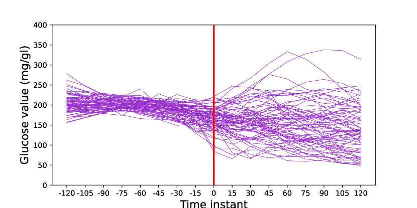
(a) Cluster 4

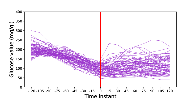
(b) Cluster 10

Figure 6: Representation of glucose over time for clusters 4 and 10.

4.4 Training, validation and Test Split

For each one of the k clusters, a first division is made into two groups, test with one-third of the cases and, on the other hand, validation-training with the remaining two-thirds. This division will be performed only once, and the same for all the techniques in this article. The validation-training set is then divided into validation, with one-third of the cases in the subgroup and the rest for training.

In Table 2, we show the total number of cases for each cluster and the division for training and testing.

Cluster	Total	Training-validation	Test
1	99	66	33
2	92	61	31
3	21	14	7
4	75	50	25
5	143	95	48
6	137	91	46
7	44	29	15
8	162	108	54
9	16	10	6
10	75	50	25
11	23	15	8
12	108	72	36
13	183	122	61
14	171	114	57
15	95	63	32

Table 2: Division of the cases of each cluster between training and test

4.5 Modeling

The process for obtaining the results is similar to the other two techniques.

In Figure 7, cluster N is divided into subsets to obtain the results for ISIGE. The process consists of three stages: training, validation, and testing. During the training phase, 30 runs are performed, and the best model for each run is selected based on the mean RMSE (MRMSE) for different segments. In the validation stage, a single model is chosen, and in the testing phase, we obtain the results of the technique for cluster N. This process is repeated for all clusters to obtain a model for each cluster.

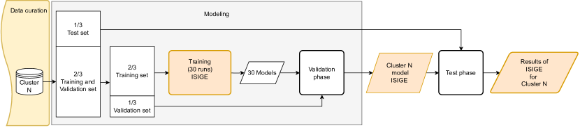
Figure 7: Generation of the results $\epsilon\text{-Lexicase ISIGE}$ for cluster N. Division of cluster N into training, validation and test sets used in the homonymous phases.

In addition to our proposal (ISIGE) and SINDy, we have experimented ANNs. As we have already stated, blood glucose prediction is an important and complex task, and ANNs have been proven valuable tools in the last years. In a recent literature review on glucose and hypoglycemia prediction methods using data from real patients [3], the authors found that ANNs, particularly recurrent neural networks (RNN) and hybrid models, performed well in predicting glucose levels. Moreover, many software tools in different languages are available on the market, and their use is increasingly ubiquitous in all kinds of problems, making them a recommendable option for the problem of blood glucose level prediction. In another study [5], the performances of several neural network models were compared for predicting blood glucose in patients with diabetes. Following the findings of the previous study, we have chosen, for this work, three ANNS models: Meijner [37], Mirshekarian [38], and Sun [39].

Based on our experimental findings and comparative analysis, it was determined that the ANN version developed by Mirshekarian exhibited superior performance. Therefore, to clearly represent ANNs, only the outcomes for the model of Mirshekarian will be showcased for comparison with SINDy and ISIGE.

5 Experimental Results

The methods studied in this work are ANNs, particularly of the Mirshekarian type, SINDy, and ISIGE, and their performance is compared with a simple baseline that is calculated by taking the mean of the glucose values at each time step over the segments of the training set.

5.1 MRMSE Results

Table 3 shows the MRMSE in the test for each method and all clusters.

The MRMSE values of SINDy and SGE are lower than the values for the mean prediction in most cases. The average MRMSE in all clusters is 38.96 [mg/L] and 37.79 [mg/L], respectively. The best values for each cluster and the best mean are marked.

Cluster ID	# Segments	Mean pred.	ANN	SINDy	ISIGE
$1$	$99$	$42.14$	$45.67$	$52.52$	41.17
$2$	$92$	$38.85$	$43.56$	$35.45$	32.81
$3$	$21$	50.25	$52.58$	$55.65$	$55.03$
$4$	$75$	$43.63$	$47.05$	$44.42$	42.87
$5$	$143$	$30.15$	$32.14$	$28.73$	26.43
$6$	$137$	$24.75$	$26.96$	22.42	23.04
$7$	$44$	$53.84$	$62.53$	44.52	48.14
$8$	$162$	$37.20$	$38.73$	30.78	32.44
$9$	$16$	$71.29$	$81.12$	44.82	45.98
$10$	$75$	$36.34$	$36.44$	$30.22$	29.92
$11$	$23$	43.50	$46.08$	$45.87$	50.48
$12$	$108$	$53.33$	$53.17$	$50.27$	48.65
$13$	$183$	$36.17$	$37.39$	$34.81$	34.18
$14$	$171$	$32.95$	$34.94$	$31.50$	30.97
$15$	$95$	$27.08$	$30.34$	$32.41$	24.72
Avg.	$96.27$	$41.43$	$44.58$	$38.96$	$37.79$

Table 3: MRMSE (mg/L) for the test set for all methods and clusters.

5.2 Parkes Error Grid Analysis

To measure the error of these techniques, we should not only look at the MRMSE. Since we are dealing with a clinical problem, it is necessary to take into account the clinical consequences. An established method for assessing errors made by blood glucose estimation or prediction systems is the Parkes Error Grid (PEG), [40]. In the PEG the actual value of blood glucose and the predicted values are plotted on a grid and associated with risk levels. These levels go from A to E and are described in Table 4.

Zone	Description
A	The actual value and the predicted value are similar.
B	Does not lead to any action by the patient or leads to benign treatment.
C	Overcorrection of acceptable blood glucose levels
D	Dangerous failure to detect and treat errors
E	Erroneous treatment, contradictory to that actually needed

Table 4: Parkes error grid zones.

For this work we use the version of PEG designed for type-I diabetes [40].

Table 5 shows the percentage of cases in each of the zones of the PEG, for each method and divided by clusters. Zone E has been omitted, since its value was zero for all methods in all clusters. Analyzing the results, most of the points are in zones A and B in all the methods, with SINDy standing out as the method with the highest mean number of points in zone A, 59.0%, and with a total of 92.4% when adding the means of zones A and B. In addition, we must also highlight the results obtained by ISIGE, achieving 93.6 % in total for the sum of the averages of zones A and B. As we move away from zones A and B, the predictions made put the patient at greater risk, with C being not very recommendable, D potentially dangerous, and E leading to an erroneous and extremely dangerous treatment. In this aspect, the models have an average percentage below 10% in zone C, with SGE standing out with only 6.2%. In the case of zone D, SINDy and ISIGE, are below 1.0%, with the lowest being ISIGE, with an average of only 0.2% of the points in this zone.

		Mean prediction				Mirshekarian (ANN)				SINDy				ISIGE
Cluster	Test segments	A	B	C	D	A	B	C	D	A	B	C	D	A	B	C	D
1	33	48.5	42.4	8.1	1	43.2	46.6	9.1	1.1	45.5	39.8	14.8	0	48.5	42.8	8.7	0
2	31	55.2	40.9	2.9	1.1	48.8	45.6	3.6	2.0	58.1	38.3	3.2	0.4	59.7	35.9	4.4	0
3	7	76.2	23.8	0	0	60.7	35.7	3.6	0	76.8	14.3	8.9	0	60.7	39.3	0	0
4	25	51.6	36.9	8.9	2.7	43.0	43.5	11.0	2.5	43.0	42.5	13.0	1.5	50.5	38.0	10.5	1
5	48	57.2	30.3	12.5	0	50.0	34.9	14.6	0.5	60.7	35.4	3.9	0	64.1	31.0	4.9	0
6	46	61.6	33.1	5.3	0	61.7	33.7	4.6	0	70.1	25.5	4.3	0	71.2	26.9	1.9	0
7	15	67.4	28.1	3.7	0.7	52.5	40.8	5.8	0.8	70.8	25.0	3.3	0.8	66.7	27.5	5.0	0.8
8	54	51	40.1	8.8	0	47.2	43.3	9.5	0	59.3	36.3	4.4	0	56.7	36.3	6.9	0
9	6	59.3	27.8	7.4	5.6	41.7	45.8	6.2	6.2	62.5	31.3	2.1	4.2	62.5	31.2	6.2	0
10	25	42.2	45.8	11.1	0.9	44.0	42.5	13.0	0.5	63.5	27.0	8.0	1.5	56.5	35.0	8.5	0
11	8	52.8	38.9	6.9	1.4	42.2	51.6	4.7	1.6	54.7	40.6	4.7	0	50.0	34.4	15.6	0
12	36	46.9	40.1	9.6	3.4	43.8	39.9	12.5	3.8	46.9	43.8	7.3	2.1	48.6	41.7	8.0	1.7
13	61	56.8	34.6	8.6	0	52.3	38.3	9.4	0	55.3	36.1	8.4	0.2	59.2	33.4	7.2	0.2
14	57	59.8	36.1	4.1	0	55.9	39.3	4.6	0.2	63.2	33.3	3.5	0	62.9	34.2	2.9	0
15	32	61.1	30.2	8.7	0	57.8	30.9	11.3	0	55.1	32.0	11.3	1.6	65.2	32.8	2.0	0
Mean	32.3	56.5	35.3	7.1	1.1	49.7	40.8	8.2	1.3	59.0	33.4	6.7	0.8	58.9	34.7	6.2	0.2

Table 5: Percentage of prediction / measurement pairs in the Parkes error zones by cluster and method

Figure 8 shows the PEG error zones for all the clusters and all methods. We can see that most of the points are located between zones A and B. To a minor amount, we can find points in zones C and D, particularly in the left zone of the grid. This zone is related to the actual values associated with hypoglycemia (values below 70), those predictions that give a high glucose value being in this zone are potentially dangerous, so it is of great interest to avoid these situations. On the other hand, it is easier to detect hypoglycemic values compared to hyperglycemic ones.

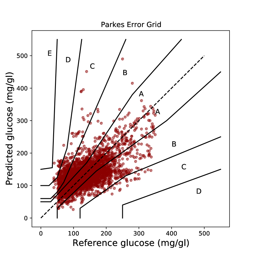
(a) SINDy

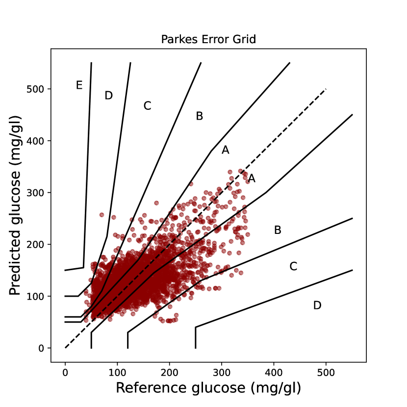
(b) ISIGE

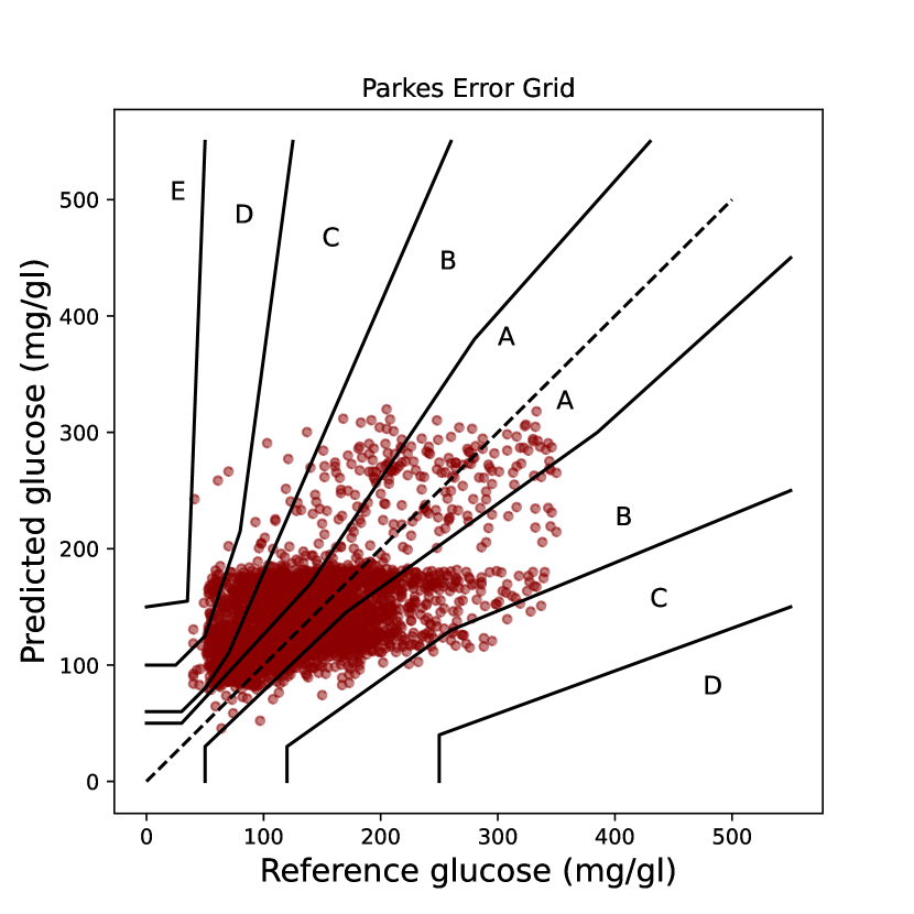
(c) Mirshekarian

Figure 8: Plot showing the PEG for each method and all clusters.

One of the advantages of using FDEs is that we can obtain forecasting for several time steps. In this work, eight steps predictions are made for each segment,(i.e. forecast horizon of 2 hours in 15-minute steps). In Figure 9 we show the distribution of points in the different zones of the PEG. Three divisions have been made by joining zones of the PEG, A + B (green), C (orange), and D + E (dark red). The x-axis shows the time horizon, and the y-axis shows the percentage of glucose prediction and measurement pairs in each zone.

By comparing the percentage of cases in zones A and B obtained by each of the techniques for each time horizon, we can see that the lowest value is around 80% for our proposal, 70% for SYNDy and 60% for Mirshekarian.

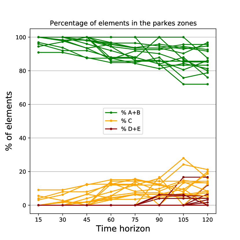
(a) SINDy

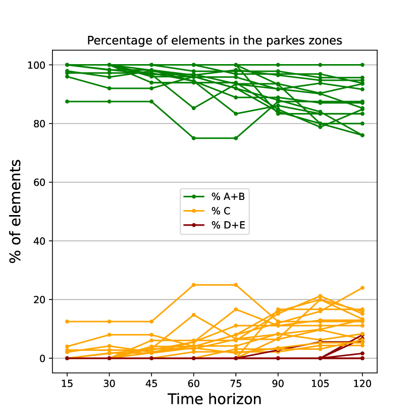
(b) ISIGE

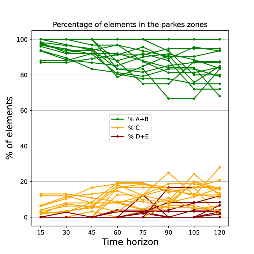
(c) Mirshekarian

Figure 9: Plot showing the percentage of elements in the different Parkes Error Grid zones for each method and all clusters.

In Figure 9(b) for SGE, most points are concentrated in zones A and B at the beginning. The further we move away from the initial time instant, the more points appear in zone C and finally reach zone D. This behavior can be explained due to the increasing difficulty of the prediction for longer forecast periods.

Currently, predictions are made at 15 minutes step, but applying the same methodology makes it possible to modify this interval depending on the frequency with which the data have been collected on CGM system. The Parkes error Grid of each time step for all methods is attached in A.

5.3 Expressions and interpretability

The interpretability of machine learning models is a topic of significant interest, yet a consensus on its definition, quantification, and measurement remains elusive. Complexity, transparency, and the ability to be simulated are among the key characteristics often associated with interpretability. However, interpretations may vary depending on the perspective of the evaluator, with mathematicians and healthcare professionals likely to have differing opinions on the same model. In this study, focusing on the healthcare domain, we specifically examine the transparency of models as a crucial aspect of interpretability. Based on the work of Lipton (2018)[41] and Belle (2021) [42], three dimensions are proposed to analyze model transparency: simulatability, decomposability, and algorithmic transparency.

• Simulatability refers to the capacity of the model to be simulated by a human, with simplicity and compactness being key attributes. Simple and compact models are more likely to fall into this category. However, it is essential to note that more than simplicity alone is required, as an excessive number of simple rules can hinder the ability of a human to mentally calculate the decisions of the model. Conversely, some complex models, such as neural networks without hidden layers, may still exhibit simulatability.

• Decomposability entails breaking down the model into interpretable parts, including inputs, parameters, and computations, and subsequently explaining each component. Unfortunately, not all models satisfy this property, making it challenging to explain their inner workings comprehensively.

• Algorithmic transparency focuses on understanding the procedural steps employed by the model to generate its outputs. Models that employ clear procedures, such as similarity-based classifiers like K-nearest neighbours, exhibit algorithmic transparency. On the other hand, complex models like neural networks construct elusive loss functions, and the solution to the training objective often requires approximation. Inspecting the model through mathematical analysis is the primary requirement for it to fall into this category.

Some models inherently possess one or more of these qualities, making them candidates for transparent models. For example, logistic/linear regression models used to predict continuous and categorical targets, where the target is a linear combination of variables, can be considered transparent due to their clear modelling choices. However, to maintain transparency, such models must be limited, and the variables used should be understandable to the intended users. The complexity of the model is directly linked to its transparency. Even if a model satisfies several transparency dimensions, a highly complex procedure or a large number of dimensions can render the model less interpretable.

The definition of transparency by Lipton and Belle aligns with the models obtained by SINDy and ISIGE, suggesting their transparency and explainability. Evaluating the complexity of these models confirms their interpretability, although SINDy models with numerous terms may pose challenges in interpretation due to the increased complexity introduced.

Table 6 presents the expressions obtained by ISIGE for the different clusters. Notably, a consistent element observed across all expressions is the inclusion of $G(t_{n})$ at the beginning. This common occurrence arises from the grammar utilized during the expression generation process, ensuring that all the expressions obtained conform to the form of FDEs. By imposing this starting point, the resulting expressions adhere to the desired mathematical structure.

To facilitate comprehension of the expressions, they have been simplified using the Python sympy library [43], which enables a more accessible understanding of the obtained mathematical representations. The employment of this library aids in unraveling the complexity of the expressions and enhances their interpretability.

The recurrent occurrence of the variable HR in the expressions is interesting. Previous studies (Rothberg et al., 2016) [44], have extensively investigated the correlation between heart rate and blood glucose levels, establishing a solid connection between these variables. Therefore, the presence of HR in the expressions is justified, considering its established relationship with the target variable. Additionally, it is worth noting that HR often co-occurs with carbohydrate intake in the expressions. This frequent association suggests a potential connection between heart rate, carbohydrate intake, and the target variable. This observation raises intriguing possibilities for future research, as it could provide valuable insights into the relationship among these variables. Further investigations in this direction may be warranted to explore and uncover the significance of this relationship. Furthermore, it is interesting to highlight that in the solution of cluster number 8, the expression includes terms for carbohydrate intake and HR, while the term for insulin bolus is absent. This solution demonstrates satisfactory performance due to the time series behaviour of the cluster. Nevertheless, this finding calls for specialized clinicians to conduct in-depth studies and assess the validity and applicability of such a solution. However, thanks to the transparency of the model, a healthcare specialist could choose to replace this expression with another one that obtained a good result in the validation phase.

Cluster	Expression
1	$G(t_{n+1})=G(t_{n})-I_{B}(t_{n})\cdot C(t_{n})+I_{B}(t_{n})-F_{ch}(t_{n})\cdot G(t_{n})+4.6$
2	$G(t_{n+1})=G(t_{n})+I_{B}(t_{n})\cdot\text{HR}(t_{n})-G(t_{n})^{2}/4000+1/(I_{B}(t_{n})\cdot\text{HR}(t_{n}))$
3	$G(t_{n+1})=G(t_{n})-49\cdot I_{B}(t_{n})\cdot\text{HR}(t_{n})/10+F_{ch}(t_{n})\cdot G(t_{n})-F_{ch}(t_{n})\cdot S(t_{n})+1/(F_{ch}(t_{n})^{2}\cdot G(t_{n})^{2})$
4	$G(t_{n+1})=G(t_{n})-B_{I}(t_{n})\cdot C(t_{n})-2\cdot F_{ch}(t_{n})\cdot G(t_{n})+F_{ch}(t_{n})\cdot\text{HR}(t_{n})+7.8$
5	$G(t_{n+1})=G(t_{n})-B_{I}(t_{n})\cdot G(t_{n})+B_{I}(t_{n})\cdot\text{HR}(t_{n})-I_{B}(t_{n})\cdot\text{HR}(t_{n})+9.9$
6	$G(t_{n+1})=G(t_{n})+2\cdot I_{B}(t_{n})\cdot C(t_{n})-I_{B}(t_{n})\cdot G(t_{n})-F_{ch}(t_{n})\cdot G(t_{n})+8$
7	$G(t_{n+1})=G(t_{n})-I_{B}(t_{n})\cdot S(t_{n})+49/5-G(t_{n})/C(t_{n})$
8	$G(t_{n+1})=G(t_{n})-F_{ch}(t_{n})\cdot\text{HR}(t_{n})+3.6$
9	$G(t_{n+1})=G(t_{n})-C(t_{n})\cdot F_{ch}(t_{n})\cdot(-5\cdot I_{B}(t_{n})\cdot F_{ch}(t_{n})\cdot\text{HR}(t_{n})^{2}+5\cdot F_{ch}(t_{n})+91)/5$
10	$G(t_{n+1})=G(t_{n})-I_{B}(t_{n})\cdot G(t_{n})+F_{ch}(t_{n})\cdot\text{HR}(t_{n})+3.9$
11	$G(t_{n+1})=G(t_{n})+B_{I}(t_{n})\cdot C(t_{n})-I_{B}(t_{n})\cdot C(t_{n})-I_{B}(t_{n})\cdot G(t_{n})-1/(I_{B}(t_{n})\cdot\text{HR}(t_{n}))$
12	$G(t_{n+1})=G(t_{n})+B_{I}(t_{n})\cdot C(t_{n})-I_{B}(t_{n})\cdot C(t_{n})-I_{B}(t_{n})\cdot G(t_{n})-F_{ch}(t_{n})\cdot G(t_{n})+2.4$
13	$G(t_{n+1})=G(t_{n})-I_{B}(t_{n})\cdot G(t_{n})-F_{ch}(t_{n})\cdot G(t_{n})+F_{ch}(t_{n})\cdot\text{HR}(t_{n})+9.49989$
14	$G(t_{n+1})=G(t_{n})-I_{B}(t_{n})\cdot C(t_{n})+C(t_{n})\cdot F_{ch}(t_{n})-F_{ch}(t_{n})\cdot G(t_{n})+5.9$
15	$G(t_{n+1})=G(t_{n})-B_{I}(t_{n})\cdot G(t_{n})+B_{I}(t_{n})\cdot\text{HR}(t_{n})-I_{B}(t_{n})\cdot\text{HR}(t_{n})+7.3027$

Table 6: Expressions for each cluster using ISIGE

In this section we only discuss the expressions obtained by ISIGE, but in Appendix 7 we attach those obtained by SINDy.

6 Conclusion and future work

In conclusion, this paper proposes a novel approach to glucose prediction in diabetes management that emphasises interpretability: Interpretable Sparse Identification by Grammatical Evolution (ISIGE). The proposed technique combines clustering with ISIGE to obtain finite difference equations that predict postprandial glucose levels up to two hours after meals.

In this study, we have employed data from 24 different participants with diabetes mellitus type-I. The data were divided into four-hour segments with two hours before and two hours after a meal, i.e. carbohydrate intake. Clustering was performed based on the blood glucose values for the two-hour window before the meal, dividing the cases into 15 clusters. Forecasts were calculated for the two-hour window after the meal. The results of the newly proposed method are compared to SINDy and artificial neural networks (ANN).

Using Parkes Error Grid to quantify the safety and robustness of the predictions, the essential conclusions of this work are:

• Predictions produced by comparison methods (SINDy and ANNs) are in zones A and B, indicating that the predictions of these models are generally safe. ISIGE achieves 93.6 % predictions in zones A and B, which is the highest among all methods.

• SINDy has the highest number of predictions (59 %) in zone A, and 92.4 % in either zone A or B.

• All models have fewer than 10 % of predictions in zone C, with ISIGE standing out with only 6.2 %. SINDy and ISIGE have below 1.0 % of predictions in zone D, with the lowest being ISIGE, with an average of only 0.2 %. None of the studied methods has predictions in zone E.

• Although only few predictions are in zones C and D, they represent a risk for participants and should be monitored.

We have used the Mean root mean square error (MRMSE) to quantify the accuracy of the predictions. In this sense, the conclusions are:

• The average MRMSE over all clusters is 38.96 [mg/L] for SINDy and 37.79 [mg/L] ISIGE. The results indicate that the models have different performance levels across different clusters.

• Although ANN is one of the best-performing techniques for glucose prediction and one of the most commonly used methods in this field, in our study, both SINDy and ISIGE obtained better results in most clusters.

Transparency plays a pivotal role in enhancing the interpretability of machine learning models in the healthcare domain. By focusing on the dimensions of simulatability, decomposability, and algorithmic transparency, we can assess and analyze the transparency of models. Transparent models exhibit simplicity, compactness, and transparent procedures, making them more amenable to human understanding. The insights gained from this study provide valuable guidance for future developments in interpretability, helping to advance the explainability of machine learning models in healthcare and beyond. We conclude that ISIGE can potentially assist diabetes clinicians in developing personalised treatment plans for their patients, offering a promising alternative to traditional black-box models like ANNs.

Appendix A Parkes Error Grid per time horizon

Parkes Errors Grid by Time Horizon for $\epsilon$Lexicase ISIGE, all clusters, figures 10 and 11.

(a) Time horizon 15

(b) Time horizon 30

(c) Time horizon 45

(d) Time horizon 60

Figure 10: Parkes Errors Grid by Time Horizon for ISIGE, all clusters (part 1).

(a) Time horizon 75

(b) Time horizon 90

(c) Time horizon 105

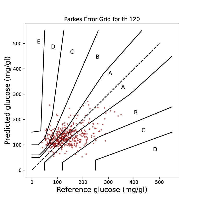
(d) Time horizon 120

Figure 11: Parkes Errors Grid by Time Horizon for ISIGE, all clusters (part 2).

Parkes Errors Grid by Time Horizon for SINDy, all clusters, figures 12 and 13.

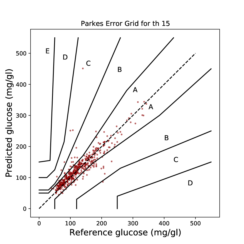
(a) Time horizon 15

(b) Time horizon 30

(c) Time horizon 45

(d) Time horizon 60

Figure 12: Parkes Errors Grid by Time Horizon for SINDy, all clusters (part 1).

(a) Time horizon 75

(b) Time horizon 90

(c) Time horizon 105

(d) Time horizon 120

Figure 13: Parkes Errors Grid by Time Horizon for SINDy, all clusters (part 2).

Parkes Errors Grid by Time Horizon for SINDy, all clusters, figures 14 and 15.

(a) Time horizon 15

(b) Time horizon 30

(c) Time horizon 45

(d) Time horizon 60

Figure 14: Parkes Errors Grid by Time Horizon for Mirshekarian, all clusters (part 1).

(a) Time horizon 75

(b) Time horizon 90

(c) Time horizon 105

(d) Time horizon 120

Figure 15: Parkes Errors Grid by Time Horizon for Mirshekarian, all clusters (part 2).

Appendix B Expressions per cluster

Table 7 shows the expressions obtained by SINDy for each cluster.

Cluster	Expression
1	$G^{\prime}(t)=181.854-2706.076\cdot I_{Bg}(t)+3814.515\cdot C_{Bg}(t)-637.866\cdot B_{I}(t)-152.312\cdot T_{M}(t)\cdot I_{Bg}(t)+19.558\cdot T_{M}(t)\cdot C_{Bg}(t)$
	$+10.907\cdot T_{M}(t)\cdot B_{I}(t)+37.952\cdot I_{Bg}(t)\cdot c_{60}(t)+25.308\cdot I_{Bg}(t)\cdot H_{60}(t)-3423.206\cdot C_{Bg}(t)^{2}$
	$-73.652\cdot C_{Bg}(t)\cdot c_{60}(t)-26.789\cdot C_{Bg}(t)\cdot H_{60}(t)+2.087\cdot C_{Bg}(t)\cdot S_{60}(t)+2319.862\cdot C_{Bg}(t)\cdot B_{I}(t)$
	$+2010.550\cdot B_{I}(t)^{2}$
2	$G^{\prime}(t)=-23.920+1.026\cdot G(t-1)+4.753\cdot T_{M}(t)+4.167\cdot I_{Bm}(t)+59.537\cdot B_{I}(t)-14.457\cdot T_{M}(t)\cdot B_{I}(t)$
	$-9.834\cdot I_{Bm}(t)\cdot B_{I}(t)-14.297\cdot B_{I}(t)^{2}$
3	$G^{\prime}(t)=0.980\cdot G(t-1)+0.135\cdot T_{M}(t)\cdot G^{\prime\prime}(t-1)$
4	$G^{\prime}(t)=1.042\cdot G(t-1)-0.106\cdot H_{30}(t)$
5	$G^{\prime}(t)=9.332+1.014\cdot G(t-1)-2.449\cdot T_{M}(t)-7.165\cdot B_{I}(t)+10.019\cdot T_{M}(t)\cdot B_{I}(t)+2.430\cdot I_{Bm}(t)\cdot B_{I}(t)$
	$-70.013\cdot B_{I}(t)^{2}$
6	$G^{\prime}(t)=24.734+0.905\cdot G(t-1)-1.596\cdot T_{M}(t)+1.219\cdot I_{Bm}(t)-47.738\cdot B_{I}(t)+0.362\cdot G(t-1)\cdot B_{I}(t)$
	$-0.497\cdot T_{M}(t)\cdot I_{Bm}(t)+0.115\cdot T_{M}(t)\cdot C_{BM}(t)+1.851\cdot T_{M}(t)\cdot B_{I}(t)-0.231\cdot I_{Bm}(t)^{2}$
	$+9.336\cdot I_{Bm}(t)\cdot B_{I}(t)-0.662\cdot C_{BM}(t)\cdot B_{I}(t)+0.476\cdot c_{30}(t)\cdot B_{I}(t)-0.540\cdot H_{30}(t)\cdot B_{I}(t)$
	$-16.124\cdot B_{I}(t)^{2}$
7	$G^{\prime}(t)=0.995\cdot G(t-1)-0.243\cdot G(t-1)\cdot I_{Bg}(t)+0.130\cdot T_{M}(t)\cdot G^{\prime}(t-1)$
8	$G^{\prime}(t)=1.023\cdot G(t-1)-4.029\cdot G(t-1)\cdot C_{Bg}(t-30)+1.978\cdot G(t-1)\cdot I_{Bg}(t-45)-1.251\cdot G(t-1)\cdot C_{Bg}(t-45)+7.035\cdot H_{30}(t)\cdot C_{Bg}(t-30)$
	$-3.142\cdot H_{30}(t)\cdot I_{Bg}(t-45)$
9	$G^{\prime}(t)=1.032\cdot G(t-1)-2.572\cdot G(t-1)\cdot C_{Bg}(t)$
10	$G^{\prime}(t)=1.050\cdot G(t-1)+4.970\cdot G(t-1)\cdot I_{Bg}(t-15)-5.794\cdot G(t-1)\cdot I_{Bg}(t-30)-1.373\cdot G(t-1)\cdot I_{Bg}(t-45)$
	$-7.067\cdot H_{30}(t)\cdot I_{Bg}(t-15)+2.505\cdot H_{30}(t)\cdot C_{Bg}(t-15)+7.262\cdot H_{30}(t)\cdot I_{Bg}(t-30)$
11	$G^{\prime}(t)=1.556\cdot G(t-1)-0.916\cdot H_{30}(t)-1.497\cdot G^{\prime}(t-1)-0.218\cdot G^{\prime\prime}(t-1)-0.165\cdot G(t-1)\cdot T_{M}(t)-10.700\cdot G(t-1)\cdot I_{Bg}(t)$
	$+4.396\cdot G(t-1)\cdot C_{Bg}(t)+0.377\cdot G(t-1)\cdot B_{I}(t)+0.745\cdot T_{M}(t)^{2}+0.204\cdot T_{M}(t)\cdot H_{30}(t)+0.198\cdot T_{M}(t)\cdot G^{\prime\prime}(t-1)$
	$-9.179\cdot I_{Bg}(t)\cdot c_{30}(t)+16.677\cdot I_{Bg}(t)\cdot H_{30}(t)+2.197\cdot I_{Bg}(t)\cdot S_{30}(t)+9.326\cdot I_{Bg}(t)\cdot G^{\prime}(t-1)$
	$+4.338\cdot I_{Bg}(t)\cdot G^{\prime\prime}(t-1)-4.349\cdot C_{Bg}(t)\cdot H_{30}(t)-1.192\cdot C_{Bg}(t)\cdot S_{30}(t)-0.183\cdot S_{30}(t)\cdot B_{I}(t)$
12	$G^{\prime}(t)=1.349\cdot G(t-1)-0.644\cdot H_{30}(t)-4.321\cdot G(t-1)\cdot C_{Bg}(t)-5.870\cdot G(t-1)\cdot I_{Bg}(t-15)+1.481\cdot G(t-1)\cdot C_{Bg}(t-15)$
	$+3.010\cdot G(t-1)\cdot I_{Bg}(t-30)-2.549\cdot G(t-1)\cdot C_{Bg}(t-30)-0.995\cdot G(t-1)\cdot I_{Bg}(t-45)+0.152\cdot G(t-1)\cdot I_{Bg}(t-60)$
	$-6.401\cdot G(t-1)\cdot C_{Bg}(t-60)+5.004\cdot C_{Bg}(t)\cdot H_{30}(t)+8.597\cdot H_{30}(t)\cdot I_{Bg}(t-15)+1.356\cdot H_{30}(t)\cdot C_{Bg}(t-15)$
	$-1.164\cdot H_{30}(t)\cdot I_{Bg}(t-45)+12.415\cdot H_{30}(t)\cdot C_{Bg}(t-60)$
13	$G^{\prime}(t)=6.897+1.041\cdot G(t-1)-0.743\cdot T_{M}(t)-0.270\cdot C_{BM}(t)-0.276\cdot G(t-1)\cdot B_{I}(t)+0.235\cdot T_{M}(t)\cdot I_{Bm}(t)$
	$-1.196\cdot I_{Bm}(t)\cdot B_{I}(t)+0.845\cdot C_{BM}(t)\cdot B_{I}(t)+25.383\cdot B_{I}(t)^{2}$
14	$G^{\prime}(t)=43.211+0.968\cdot G(t-1)-1.323\cdot T_{M}(t)+8.345\cdot I_{Bm}(t)-0.442\cdot C_{BM}(t)+0.191\cdot c_{30}(t)-0.613\cdot H_{30}(t)$
	$-29.836\cdot B_{I}(t)+0.280\cdot T_{M}(t)\cdot B_{I}(t)-47.855\cdot I_{Bm}(t)\cdot B_{I}(t)+3.367\cdot C_{BM}(t)\cdot B_{I}(t)-0.426\cdot c_{30}(t)\cdot B_{I}(t)$
	$+1.669\cdot H_{30}(t)\cdot B_{I}(t)-181.578\cdot B_{I}(t)^{2}$
15	$G^{\prime}(t)=2.064+0.906\cdot G(t-1)-6.279\cdot T_{M}(t)-404.138I_{Bm}(t)+59.925\cdot C_{Bg}(t)-0.257\cdot c_{30}(t)+0.446\cdot h_{30}(t)$
	$+205.460\cdot B_{I}(t)+1.041\cdot G^{\prime}(t-1)+3.971G(t-1)\cdot I_{Bm}(t)-0.275\cdot G(t-1)\cdot C_{Bg}(t)-0.650\cdot G(t-1)\cdot B_{I}(t)$
	$+0.527\cdot T_{M}(t)^{2}+67.439\cdot T_{M}(t)\cdot I_{Bm}(t)-27.930\cdot T_{M}(t)\cdot C_{Bg}(t)+0.862\cdot T_{M}(t)\cdot B_{I}(t)+2600.891\cdot I_{Bm}(t)^{2}$
	$+3515.204\cdot I_{Bm}(t)\cdot C_{Bg}(t)+9.307I_{Bm}(t)\cdot c_{30}(t)-10.954\cdot I_{Bm}(t)\cdot h_{30}(t)-0.281I_{Bm}(t)\cdot S_{30}(t)$
	$-7.904I_{Bm}(t)\cdot B_{I}(t)+4.365I_{Bm}(t)\cdot G^{\prime}(t-1)-6.653\cdot I_{Bm}(t)\cdot G^{\prime\prime}(t-1)-1085.326\cdot C_{Bg}(t)^{2}-8.024\cdot C_{Bg}(t)\cdot c_{30}(t)$
	$+3.287\cdot C_{Bg}(t)\cdot h_{30}(t)+0.523\cdot C_{Bg}(t)\cdot S_{30}(t)-15.630\cdot C_{Bg}(t)\cdot G^{\prime}(t-1)+7.066\cdot C_{Bg}(t)\cdot G^{\prime\prime}(t-1)$
	$+1.109\cdot c_{30}(t)\cdot B_{I}(t)-1.826\cdot h_{30}(t)\cdot B_{I}(t)-128.624\cdot B_{I}(t)^{2}-1.342\cdot B_{I}(t)\cdot G^{\prime}(t-1)$

Table 7: Expressions for each cluster using SINDy

References

- [1] S. Mirshekarian, H. Shen, R. Bunescu, C. Marling, Lstms and neural attention models for blood glucose prediction: Comparative experiments on real and synthetic data, in: 2019 41st annual international conference of the IEEE engineering in medicine and biology society (EMBC), IEEE, 2019, pp. 706–712.
- [2] C. Cobelli, A. Mari, Validation of mathematical models of complex endocrine-metabolic systems. a case study on a model of glucose regulation, Med. Biol. Eng. Comput. 21 (4) (1983) 390–399.
-
[3]
V. Felizardo, N. M. Garcia, N. Pombo, I. Megdiche,
Data-based
algorithms and models using diabetics real data for blood glucose and
hypoglycaemia prediction – a systematic literature review, Artificial
Intelligence in Medicine 118 (2021) 102120.
doi:https://doi.org/10.1016/j.artmed.2021.102120.
URL https://www.sciencedirect.com/science/article/pii/S0933365721001135 -
[4]
S. Contador, J. M. Velasco, O. Garnica, J. I. Hidalgo,