Rockmate: an Efficient, Fast, Automatic and Generic Tool
for Re-materialization in PyTorch

Abstract

We propose Rockmate to control the memory requirements when training PyTorch DNN models. Rockmate is an automatic tool that starts from the model code and generates an equivalent model, using a predefined amount of memory for activations, at the cost of a few re-computations. Rockmate automatically detects the structure of computational and data dependencies and rewrites the initial model as a sequence of complex blocks. We show that such a structure is widespread and can be found in many models in the literature (Transformer based models, ResNet, RegNets,…). This structure allows us to solve the problem in a fast and efficient way, using an adaptation of Checkmate (too slow on the whole model but general) at the level of individual blocks and an adaptation of Rotor (fast but limited to sequential models) at the level of the sequence itself. We show through experiments on many models that Rockmate is as fast as Rotor and as efficient as Checkmate, and that it allows in many cases to obtain a significantly lower memory consumption for activations (by a factor of 2 to 5) for a rather negligible overhead (of the order of 10% to 20%). Rockmate is open source and available at https://github.com/topal-team/rockmate.

1 Introduction

In recent years, very large networks have emerged. These networks induce huge memory requirements both because of the number of parameters and the size of the activations that must be kept in memory to perform back-propagation. Memory issues for training have been identified for a long time. Indeed, training is usually performed on computing resources such as GPUs or TPUs, on which memory is limited. Therefore, different approaches have been proposed.

The first category of solutions consists in relying on parallelism. Data parallelism allows to distribute the memory related to the activations, at the cost of exchanging the network weights between the different resources using collective communications such as MPI_AllReduce which can be expensive for networks such as those of the GPT2 class. On the contrary, model parallelism allows to distribute the weights of the network, at the cost of the communication of activations and memory overheads in case it is used in a pipelined way, and its scalability is limited by nature.

The second category of solutions is purely sequential. Offloading makes it possible to move some activations computed during the forward phase from the memory of the accelerator (GPU or TPU) to the memory of the CPU, and then to prefetch them back at the appropriate moment into the memory of the GPU during the backward phase. This solution therefore consumes bandwidth on the PCI-e bus between the CPU and the accelerator, which is also used to load training data. Another solution, called re-materialization, consists in deleting from accelerator memory some activations computed during the forward phase and then recomputing them during the backward phase. This approach does not consume communication resources, but it does induce a computational overhead.

In the present paper, we focus on the latter re-materialization approach on a single GPU or TPU, which is sufficient in practice for the size of the networks we consider in the experiments and which can be trivially combined with data parallelism to accelerate training. In this framework, for a given memory constraint, the optimization problem consists in finding a sequence of computing, forgetting and recomputing actions which allows to perform the training for given inputs and batch sizes, while fulfilling the memory constraint and minimizing the computational overhead.

To find the optimal sequence, different approaches have been proposed. In the first approach, like in Rotor (Beaumont et al., 2019b), it is assumed that the dependencies within the model have a particular structure, typically a sequence of operations. In this case, using dynamic programming, it is possible to find the optimal order of computations in reasonable time. On the other hand, in the case where the computations performed by the model do not naturally consist in a sequence of operations, this approach requires to aggregate elementary operations into complex blocks to make the chain structure emerge. In this case, re-materialization decisions have to be made at the level of blocks, which reduces optimization opportunities. The left of Figure 1 shows the graph of a GPT-like model, where each block corresponds to one half of a transformer block. On such a graph, this approach has to decide during the forward phase whether to keep all internal activations or to delete all of them (and to recompute them during the backward phase).

Figure 1: Simplified example of running Rockmate on a GPT model. Left: Dependency graph of the first part of the model, where transformer blocks are shown in gray, and Rockmate blocks are identified in red. Right: (top) a schedule corresponding to the first three blocks; (bottom) indication of which activations are saved (green) or not (white) for each block, and the intervals during which they are present in memory. Saving fewer activations leads to more recomputation and thus longer backward time.

In the case of general graphs that are not structured as a sequence of elementary operations, another approach has been proposed in Checkmate (Jain et al., 2020). It consists in describing the operations corresponding to both forward and backward phases as a Directed Acyclic Graph (DAG) and to find the optimal solution through solving an Integer Linear Program (ILP). The number of integer variables is proportional to $V\times E$, where $V$ is the number of operations and $E$ is the number of arcs of the DAG. Hence, a major shortcoming of this approach is the computational time induced by solving the ILP. Typically, even using commercial solvers such as CPLEX or Gurobi, it is not possible (in one day of computation) to consider GPT2 models with more than 10 transformer blocks (see Figure 2), while classical instances include several dozens.

In the present paper we propose Rockmate, a new re-materialization strategy, in which models are seen as a sequence of blocks (in the sense of Rotor), but where several optimal strategies are pre-computed for each block (using a Checkmate-like approach). A simple example of the resulting execution is shown on the right of Figure 1, where in each block, a different set of activations is saved, resulting in different backward execution times. In reality, for a GPT model, Rockmate divides each block into 9 or 6 operations for the first or second half of the transformer block respectively, and the execution can also contain re-executions of some blocks.

As our experimental results demonstrate, for a large variety of networks Rockmate can compute near-optimal solutions (close to Checkmate quality in terms of throughput) in a reasonable time (close to Rotor runtime, faster than Checkmate), by combining the advantages of both approaches. A preview shown on Figure 2 presents the throughput and solving time of all three solutions for GPT neural networks with varying number of transformer blocks.

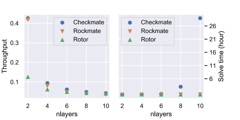
Figure 2: Efficiency comparison between Rockmate, Rotor and Checkmate for GPT2 networks with $nlayers$ transformer blocks. Rockmate finds an optimized re-materialization solution as quickly as Rotor while keeping a similar performance as Checkmate in terms of resulting throughput. Throughput is defined as the number of samples processed per time unit (ms).

Another contribution is that we have built a framework, which can be easily applied on any PyTorch nn.Module. It contains complete implementation of our algorithm (Algorithm 1), including main phases with newly proposed computation-data graph builder, integer linear programming, and dynamic programming techniques described in section 3. Rockmate takes the model as input and automatically builds the data-flow graph with measurements (computation time, output size and peak memory of each operation, etc.). The optimal schedule is then determined based on the graph and used to build a new nn.Module which runs forward and backward phases within a given memory constraint. In Section 4, we demonstrate that the resulting new GPT2 models can achieve the same result as the original ones with 25% computational overhead, while using only 25% of the original memory needs to store the activations.

Note that all the benefits of Rockmate do not induce any accuracy loss for the model: given the same batch of training data, the Rockmate model will compute exactly the same gradient values for every trainable parameter compared to the original model. Hence, both models achieve the same accuracy after the same number of training epochs.

2 Related works

During training, memory requirements are very demanding. On the one hand, they come from the storage of the network weights, and the associated intermediate data, such as gradients and optimizer states. On the other hand, memory requirements also come from the storage of the activations associated with gradient descent, since (almost) all the results computed during the forward phase must be kept in memory until they are used by the gradient computation during the backward phase.

There are different strategies for saving memory when training Deep Neural Networks (DNNs), adapted to these different memory requirements. We can differentiate between strategies that rely on the use of parallelism (data parallelism, model parallelism), those that use the possibility of transferring data to another device than the memory of the accelerator (denoted as offloading or paging in the literature), and those that rely on the redundant computation of activations deleted from the memory (denoted as checkpointing or re-materialization in the literature). Of course, these strategies can naturally be combined since they rely on different resource consumption (use of several computing resources for parallelism, external storage for offloading or re-computations for re-materialization). This combination is more or less difficult because some resources are consumed by several approaches (computations on the GPU or the TPU of course, but also communications on the PCI-e bus or on the NVLink). In the rest of this section, we will focus mainly on re-materialization strategies after having briefly discussed the other approaches.

Among the most popular parallel strategies for DNN training are data parallelism and model parallelism. Data parallelism is based on the idea of performing forward and backward phases in parallel on different data and on several GPUs. The gradients computed on the different GPUs must then be reduced, which requires collective communication of all the weights. This approach used in isolation was very popular in more or less synchronous (Zinkevich et al., 2010; Das et al., 2016) or asynchronous (Zhang et al., 2013) variants for convolutional networks in which the network weights were small compared to the activations, but is nowadays mainly used in combination with model parallelism. Model parallelism consists in distributing layers and weights over different resources and communicating forward activations and their gradients between GPUs. This approach has been popularized in frameworks like GPipe (Huang et al., 2019), Pipedream (Narayanan et al., 2019) or Varuna (Athlur et al., 2022) and its complexity has been studied in (Beaumont et al., 2021b). It is often combined with systematic re-materialization such as in GPipe (Huang et al., 2019).

Offloading (sometimes denoted as paging) can be applied to both network weights and activations. The idea is simply to remove the memory load from the GPU and store data in CPU memory, that is typically much larger than GPU memory. This idea is relevant both for activations, computed during the forward phase but which will not be used for a long time by the backward phase (Rhu et al., 2016; Le et al., 2018; Beaumont et al., 2020a) and for network weights (Beaumont et al., 2022), which are also used only once during the forward phase and once during the backward. Offloading can also be combined with re-materialization (Beaumont et al., 2021a), which is particularly relevant for decentralized training on tiny devices (Patil et al., 2022).

Historically, re-materialization strategies have their origins in the checkpointing techniques developed in the context of automatic differentiation (AD). Because of this application context, these works have focused mainly on the case of homogeneous chains, i.e. models consisting of a sequence of identical blocks. In this context, it is possible to rely on dynamic programming to find optimal solutions and even closed form formulas can be derived to automatically find the activations to keep and the ones to delete. From the complexity point of view, it has been shown that the problem is NP-complete as soon as one considers graphs more general than chains in (Naumann, 2008). In the re-materialization literature dedicated to DNN training, we can distinguish approaches that focus on the case of sequential models and those that consider more general graphs.

In the case of sequences, in (Chen et al., 2016), the sequence on length $N$ is divided into $\sqrt{N}$ equal-length segments of length $\sqrt{N}$, and only the input of each segment is materialized during the forward phase. This strategy is implemented in PyTorch in torch.utils.checkpoint.

Rotor (Beaumont et al., 2019b, a) provides optimal solutions in the case of fully heterogeneous sequential models. Rotor is based on the evaluation of the parameters of each block the sequence (computational and memory costs), on the resolution of the re-materialization problem using dynamic programming and on the implementation of the resulting computation sequence. Rotor is fast, but it is limited to sequential models. It is one of the two ingredients (with Checkmate (Jain et al., 2020) described below) of the present contribution.

Other contributions target more general graphs. For example, the approach described in (Kumar et al., 2019) is based on the computation of a tree-width decomposition of the graph to determine the minimum computational cost associated with the minimum possible memory footprint. In (Kusumoto et al., 2019), an enumeration of subgraphs is required to design efficient re-materialization strategies. In general, finding the evaluation order of the graph that minimizes the memory consumption is a hard problem, independently of any re-materialization strategy, as demonstrated in (Steiner et al., 2022). The case of (non-optimal) dynamic re-materialization, especially in the case where the input size in unknown in advance, has been addressed in (Kirisame et al., 2020; Liao et al., 2022). An important contribution in the case of general graphs has been provided in Checkmate (Jain et al., 2020), which proposes an Integer Linear Program (ILP) to find the optimal re-materialization sequence for general graphs, which is consistent with the NP-Completeness results of (Naumann, 2008). An important limitation of Checkmate (see Section 3) is the long solving time of the ILP solver, which limits its use to relatively small graphs. This paper addresses this limitation of Checkmate by proposing to combine it with Rotor.

3 Rockmate

3.1 Sketch of the Algorithm

As explained in Section 1, the main idea of this paper is to combine the ideas of (i) Checkmate, which finds good solutions in the case of general graphs but is slow, and (ii) Rotor, which finds the optimal solution only in the case of sequential networks, but is fast.

The GPT neural networks used as motivational example above is not completely sequential, but it can be decomposed in a sequence of blocks, where each block contains several operations. It is a typical example where, in order to use Rotor, it is necessary to aggregate all the operations of the same block together. Rotor therefore decides at the scale of the whole block whether to keep all the data or to delete them all during the forward phase. Checkmate, on the other hand, sees the whole graph describing the model and can therefore decide, independently and at the level of each operation, whether to keep its data or not.

The solution we propose is called Rockmate; a pseudo-code is provided in Algorithm 1 and explained below. The main idea is to apply Checkmate inside each block and to apply Rotor on the complete sequence of blocks. For this purpose, it is necessary to obtain the complete graph of all operations of the neural network, and to adapt both Checkmate and Rotor to this new setting.

Algorithm 1 Rockmate

1:  Input: $module$, $input$, $M_{GPU}$

2:  $[blocks]$ = rk-GB($module$, $input$)

3:  $budgets$ = $[(M_{peak},M_{save})]$ (quantized)

4:  $sols$ = []

5:  for all $b\in[blocks]$ do

6:     for all  $(M_{peak},M_{save})\in budgets$ do

7:        $sols[b]$.add(rk-Checkmate($b$, $M_{peak}$, $M_{save}$))

8:     end for

9:  end for

10:  $Sequence$ = rk-Rotor($sols$, $M_{GPU}$)

11:  $rkMod$.forward = rk-Exec($Sequence.fwd$)

12:  $rkMod$.backward = rk-Exec($Sequence.bwd$)

13:  Output: $rkMod$

The first phase is called rk-GB (for GraphBuilder). It occurs on line 2 of Algorithm 1 and is described in more details in Section 3.2. rk-GB takes as input a model expressed as a PyTorch nn.Module and automatically (i) extracts the Directed Acyclic Graph (DAG) of all the operations performed in the model, (ii) divides it into a sequence of blocks and (iii) detects all the blocks which have identical structures. For each unique block, the processing times of all operations and the sizes of all intermediate data that are produced by these operations are measured. These measurement (graphs of each block, labeled with the execution times and memory footprints of the produced data) contain all the necessary information to find the re-materialization sequence.

In the second phase of Rockmate (line 3-8 of Algorithm 1), we consider each single block independently. As we saw in the example in Figure 2, Rotor fails to compute very good re-materialization strategies because it can only choose between two options: keep all or delete all activations in the block. In Rockmate, we use a refined version of Checkmate to generate a larger set of re-materialization strategies. This refined version is denoted as rk-Checkmate and described in Section 3.3.

A re-materialization strategy is characterized by (i) the memory peak during the execution of the block (either during forward or backward) and (ii) the total size of the internal activations of the block that are kept between the forward phase and the backward phase. The first one ensures that this strategy can be executed within a given memory limit. The second one allows the dynamic program to know how much memory will be left for the next blocks. The number of different options to consider is a parameter of Rockmate. We analyze its effect on performance in Section 4 and show that quantizing each parameter into 20 different thresholds is enough to get good solutions in practice. This leads to at most 400 different strategies in total for each block. Since rk-Checkmate is applied at the level of a block (and not on the whole network), the corresponding graph is small enough that the runtime remains small, even for generating the whole family of strategies. Moreover, as rk-GB automatically detects identical blocks, rk-Checkmate is performed only on unique types of blocks (for instance, GPT2 models only involve five unique types of blocks). In practice, it takes less than 2 minutes to solve rk-Checkmate 400 times for a rk-block in GPT2, while it’s impossible to solve the entire network with the ILP method because of its exponential complexity.

The third phase of Rockmate (line 9 of Algorithm 1, described in Section 3.4) is called rk-Rotor and computes the global re-materialization strategy. rk-Rotor features an adapted dynamic program of Rotor that, instead of having two solutions per block, can exploit the different re-materialization strategies computed during the second phase. The output of rk-Rotor therefore consists in a schedule which describes which block should be computed, in which order, and with which re-materialization strategy. If necessary, some blocks can be computed without keeping any data at all, and thus be recomputed later (possibly several times).

Finally, the fourth phase (line 10 of Algorithm 1, described in Section 3.5) is called rk-Exec. It transforms this schedule into a new PyTorch nn.Module, which performs all the corresponding elementary operations in the correct order. The resulting module computes exactly the same gradients as the original version while respecting a global constraint on the memory usage of activations, at the cost of duplicating some computations.

3.2 Phase 1: rk-GB, Graph Builder

A typical training iteration of neural networks can be separated as forward and backward phases. Both phases can be represented by a data-flow graph. The computational graph is explicit in TensorFlow, for which Checkmate was originally implemented. In PyTorch, however, graphs need to be obtained by certain tools. We developed a tool named rk-GraphBuilder (rk-GB) which takes as input a nn.Module and an example input for it, and builds the data-flow graph of the module. Having an example input is necessary to inspect the time and memory cost of all the operations used during forward and backward phases.

Obtaining the graph

rk-GB does not require any modification or annotation of the module source code, instead it uses torch.jit to trace the forward execution of the module on the example input. This function executes the forward code and provides the list of all primitive operations used. Based on this list, we build a forward graph where each node represents one assignment. However, multiple variables may share the same memory space due to view and in-place operations in PyTorch. Such variables would thus be kept or removed together when performing re-materialization. Therefore, rk-GB merges all the nodes sharing the same memory space to obtain a simplified forward graph. For a 12-layer GPT model, the number of nodes decreases from 934 to 185 after simplification. The simplified forward graph is further cut around 1-separators: a node is a 1-separator if by removing it, we obtain a disconnected graph (1 node to separate the graph). This produces a sequence of blocks, as required by rk-Rotor. For a 12-layer GPT model, this results in 26 blocks, where each Transformer layer is separated to an Multi-Head Attention block and an MLP block.

Identical blocks

Afterwards, rk-GB goes through all the blocks to recognize identical blocks, i.e. blocks whose computational graphs are the same. Since rk-GB is deterministic, two blocks representing the same function share the same graph structure, including the same topological ordering of nodes. Following this ordering, rk-GB checks equivalency node by node. A group of identical blocks can be measured and solved together to improve the solving time. Identifying identical blocks is an optimization of the Rockmate solving time but does not change its solution quality. So even if some blocks are wrongly declared as different by Rockmate, this would not change the memory gains or the computational overhead. For a 12-layer GPT model, this procedure identifies only 5 identical blocks from the 26 rk-blocks produced after separation.

CD_graphs

One underlying assumption in the original Checkmate graph model is that each operation has exactly one output data. However, when several forward operations share the same input, the corresponding backward operations contribute to the same data (by summing all the contributions). This means that removing the result of one of these backward operations has an impact on the other operations, which can not be taken into account in the graph model of Checkmate. Additionally, some elementary operations in PyTorch actually create intermediate data (they are called saved_tensors), which can be deleted independently of the output of the operation.

For these reasons, we introduce a new graph called CD_graphs, which contain two categories of nodes: Computation and Data. A C_node represents an operation, labeled with the time it takes and the temporary memory overhead during execution. A D_node represents a data tensor stored in the memory. A D_node can be forgotten to free memory, and restored by recomputing the corresponding C_nodes. An edge between a C_node and a D_node represents the execution dependency between the operation and its output data tensors. The benefits of considering such a CD_graph is to enable finer rematerializations, such as releasing memory from a subset of outputs of one operation. The final product of rk-GB is a sequence of CD_graphs. More details about rk-GB can be found in Section A of the Appendix.

3.3 Phase 2: rk-Checkmate, Options at Block Level

Given a CD_graph, it is a non-trivial problem to find the optimal execution schedule of all the operations within a given memory limitation. To solve this problem, we use rk-Checkmate, an Integer Linear Programming (ILP) adapted from Checkmate (Jain et al., 2020). Just like Checkmate, rk-Checkmate requires a topological order of all the operations, which is provided by rk-GraphBuilder. rk-Checkmate provides several improvements over the original Checkmate formulation.

First, additional variables are introduced to represent the execution of each C_node separately from the memory allocation of each D_node. Constraints are also adapted to ensure that the execution order follows the dependencies between computational nodes and data nodes. In the case where one operation generates multiple outputs, there are multiple D_nodes depending on the same C_node. Deleting these outputs is considered separately in rk-Checkmate, whereas they are grouped together in the Checkmate formulation. For example, this improvement is useful for an operation which produces two large outputs, each required by a different operation: with rk-Checkmate, it is possible to delete the second output before performing the operation that requires the first output, which reduces the memory usage.

Second, rk-Checkmate takes into account the temporary memory usage of all operations: because of temporary data allocated and deleted during the operation, the peak memory might be higher than the size of input and output. Checkmate ignores this possibility, and thus may produce solutions whose actual peak memory is higher than the budget.

Finally, since rk-Checkmate is aware of the separation between forward and backward phases, it is possible to include a constraint on the memory usage when going from the forward to the backward phase. This constraint expresses the limit $M_{save}$ on the size of the activations which are kept in memory between both phases of a block (and thus, during the execution of the following blocks). This memory occupancy is necessary to control the overall memory cost of all the blocks. More details about rk-Checkmate can be found in Section B of the Appendix.

For each block, rk-Checkmate will be applied with different values for the memory budgets $M_{peak}$ and $M_{save}$, as explained in Section 3.1. We first compute the minimum and maximum possible values for $M_{peak}$, by analyzing the memory usage of the schedule which deletes activations as soon as possible, and of the schedule which performs no recomputation, respectively. The number of budgets is a hyperparameter of Rockmate whose effect is analyzed in Section 4.2. The values of $M_{peak}$ are evenly spaced within $[min\_peak;max\_peak]$. Given one value for $M_{peak}$, the values of $M_{save}$ are evenly spaced within $[output\_size;M_{peak}]$. This ensures that all pairs $(M_{peak},M_{save})$ given to rk-Checkmate are relevant. Note that different budgets may lead to the same optimal solution. In practice, when we apply the number of $M_{peak}$ and $M_{save}$ as (20, 20) for GPT2, there are less than 30 unique solutions per rk-block.

Note that identical blocks are solved only once with the same budgets, so that all identical blocks have the same set of block-level execution options provided to rk-Rotor. However, rk-Rotor sees all of these blocks as different parts of the sequence, which just happen to have the same set of options In the resulting sequence, each of these identical blocks may be executed with a different option in the output of rk-Rotor.

3.4 Phase 3: rk-Rotor, Global Sequence Generation.

Figure 3: Diagram representing the different cases for the dynamic program. Green arrows represent materialized activations. Green, yellow and red blocks represent internal activations to the blocks, which are respectively completely, partially, or not saved. Colored backgrounds on the subproblems represent how much memory is occupied by these activations.

Principle of Rotor

The main idea of the dynamic programming algorithm of Rotor is as follows. An optimal solution for the forward-backward computation from block $s$ to $t$ with memory $m$ can be of two different types: either the first block $s$ is computed only once, or more than once. In the first case, the computation starts with computing block $s$ and keeping all intermediate data, and continues with an optimal solution for blocks $s+1$ to $t$ (with less memory available). In the second case, the computation starts with computing blocks $s$ to $s+i$ for some $i$, stores the result of $s+i$, continues with an optimal solution for blocks $s+i$ to $t$, and finally recomputes from $s$ to $s+i$ with an optimal solution for this part. Note that no intermediate data is saved for blocks $s$ to $s+i$. An illustration of each case is represented on Figure 3.

In each case, the subproblems that need to be solved have a smaller value of $t-s$. Assuming that the solutions to these smaller problems are known, the algorithm can make the choice which leads to the smallest overhead among all valid choices, ie those for which the memory usage is not higher than the budget $m$. We can thus iteratively compute optimal solutions until we find the solution for the complete model.

rk-Rotor

In the Rockmate context, we have several different options for the first case: we can choose to keep more or less intermediate data for the first block $s$. Each of these options leads to a different memory usage for storing the intermediate data and for computing the backward operation. There is thus a larger set of choices to choose from, but the main idea is still there: assuming that solutions to all smaller problems are known, we can select the option that yields the lowest overhead among all options which respect the memory budget. This improved case is represented at the bottom of Figure 3.

Complexity analysis

With a model that contains $L$ blocks, and a memory of size $M$, the Rotor algorithm has a complexity in $O(L^{3}M)$: for each value of $s$, $t$ and $m$, there are $O(L)$ choices to consider. In the Rockmate case, with $B$ budget options, the dynamic programming algorithm considers $O(L+B)$ choices at each step, and thus has a complexity in $O(L^{2}M(L+B))$. More details about the rk-Rotor algorithm can be found in Section C of the Appendix.

Sub-optimality of the solution

Although both rk-Checkmate and rk-Rotor obtain optimal solutions for the given sub-tasks, the final Rockmate solution is not always optimal on the overall network. Two reasons can lead to sub-optimality in Rockmate: (i) since the number of memory budgets is finite, only a limited number of execution schedules are produced by rk-Checkmate. (ii) in rk-Rotor, intermediate data is only used to improve the execution time of the backward phase. However, if the forward phase of a block is executed several times, it might be beneficial to save some intermediate tensor on the first pass, and use it to compute the output faster on subsequent passes. This possibility is not considered in rk-Rotor: forward passes in case 2 do not save intermediate data.

3.5 Phase 4: rk-Exec

Rockmate creates a PyTorch nn.Module that performs a forward-backward computation based on the optimal schedule solved by the algorithm described above. The execution of the forward phase is based on the Python code obtained via jit.trace. For backward, the PyTorch autograd engine stores the “computational graph” during the forward phase, which allows backward computation from the output back to the input. For the sake of clarity, we call this an autograd graph. In Rockmate, we detach the operations during the forward phase, so that the full network is represented as many small autograd graphs. This allows the backward operations to be performed separately, thus deletions of tensors can be easily inserted between two backward operations. Specifically, rk-Exec creates one autograd graph for each C_node defined in Section 3.2. Every autograd graph contains all the operation which create tensors sharing the same memory space, such as torch.Tensor.view operations. During the backward phase, the gradient of each tensor is automatically supplied to the previous backward function. Furthermore, the recomputation of the operations have to be performed in different ways, so that the existing autograd graph will not be rebuilt. Also, when one operation will be recomputed before the backward, the execution will be with torch.no_grad mode so that saved_tensors will not be created. More details about the rk-Rotor algorithm can be found in Section D of the Appendix.

4 Experiments

4.1 Experimental Settings

All experiments presented in this paper are performed using Python 3.9.12 and PyTorch 1.13.0. Rockmate, Rotor, and Checkmate compute their solutions on a 40-core Intel Xeon Gold 6148, while training is performed on an Nvidia Tesla V100 GPU with 15.75 GB of memory. For comparison with Rotor on ResNet and GPT2, both networks are implemented as a nn.Sequential module of PyTorch. For RegNet, we do not provide a comparison with Rotor due to the lack of a Rotor-compatible implementation. All experiments use the version of Rockmate available at: https://github.com/topal-team/rockmate/releases/tag/v1.0.

Rockmate is used to reduce peak memory usage due to storage of activations. We measure and control the memory footprint of activations during the experiments. The memory used by the model parameters is excluded from our peak memory budget, as it remains constant during training. In practice, we adjust the maximum peak memory for activations by subtracting the size of the model from the total memory.

4.2 Precision

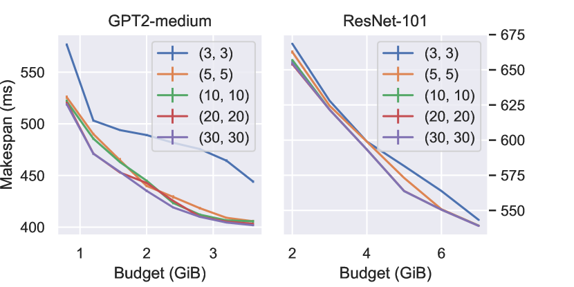
Figure 4: Experiments on GPT2-medium and ResNet-101. Number of $(M_{peak},M_{save})$ budgets are chosen from (3,3) to (30,30). Makespan is the time of one training iteration (including forward and backward).

As discussed in Section 3.3, the same number of budget options are used to solve each block in rk-Checkmate. Increasing the number of options increases the time to run Rockmate, since it is directly related to the number of times rk-Checkmate is called for each block. However, it provides finer re-materialization strategies for rk-Rotor. Figure 4 shows how the number of budget options affects the quality of the Rockmate solution. Budget options range from (3,3) to (30,30) for GPT2-medium and ResNet-101. Overall, increasing the number of budget options improves Rockmate performance up to a point. Specifically, the improvement in the Rockmate solution is stronger on GPT2-medium than on ResNet when more budget options are allowed. This is because a GPT2 block contains more complicated structures (more nodes in block), while a ResNet block is too small to apply sophisticated re-materialization strategies. In the following experiments, we use the number of $(M_{peak},M_{save})=(20,20)$ for rk-Checkmate.

4.3 Efficiency

In Figure 5, we compare the solving time and performance of Rockmate, Checkmate (Jain et al., 2020), and Rotor (Beaumont et al., 2020b) on GPT networks with 2 to 10 Transformer blocks. For each network, we choose the smallest memory budget for which we obtain feasible solutions. Checkmate is solved until convergence. Rockmate achieves very similar throughput to Checkmate, while Rotor can be significantly worse if the network is not deep enough. Since Rotor has only the option to recompute a whole block, it is more effective when the network is deep.

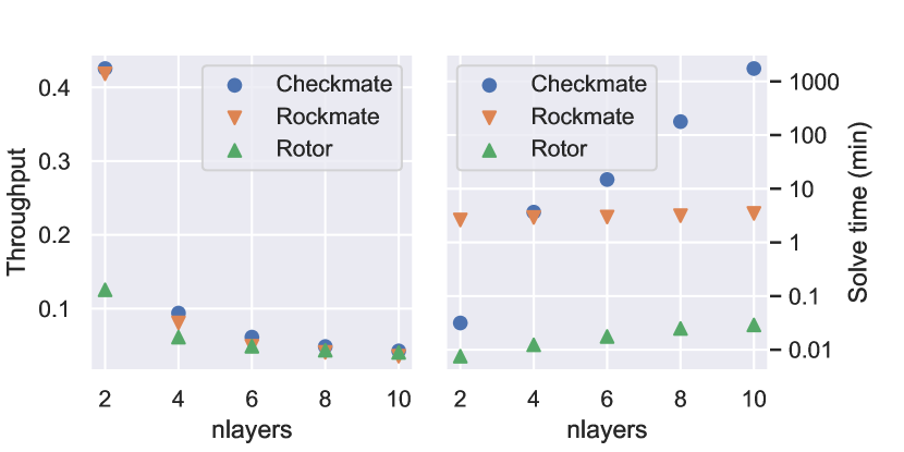
Figure 5: Experiments on solving GPT2 with 2-10 Transformer blocks with given budgets. Simulation solving time is in log scale. Throughput is defined as the number of samples processed per time unit (ms).

The time to solution of Rockmate remains nearly the same as the network gets deeper. The processing time of Rockmate consists of three parts: 1. inspection time during graph building; 2. rk-Checkmate processing time; 3. rk-Rotor processing time. As described in Section 3.2, rk-GB automatically detects identical blocks. Only one inspection is performed for a class of identical blocks, and they are solved by the same rk-Checkmate models. Therefore, the inspection time and the rk-Checkmate time remain the same when the number of identical transformer blocks increases. The rk-Rotor solving time is similar to Rotor’s, which is much faster than the total Rockmate solving time.

The complexity of Checkmate’s ILP model grows exponentially with the size of the network, making it infeasible on modern neural networks with thousands of nodes. In Figure 5 we compare the solving time and performance of Checkmate and Rockmate on GPT2 with 2 to 10 Transformer blocks. The memory budgets are chosen as the minimum achievable budgets for both models. The solving time of Checkmate is exponential in the number of blocks, exceeding 30 hours on the 10-blocks GPT2. On the other hand, the solution time of Rockmate remains almost constant because the same rk-Checkmate models are applied to all identical Transformer blocks. Despite the significant difference in solution time, Rockmate achieves similar or better overhead than Checkmate within the same budget.

4.4 Performance

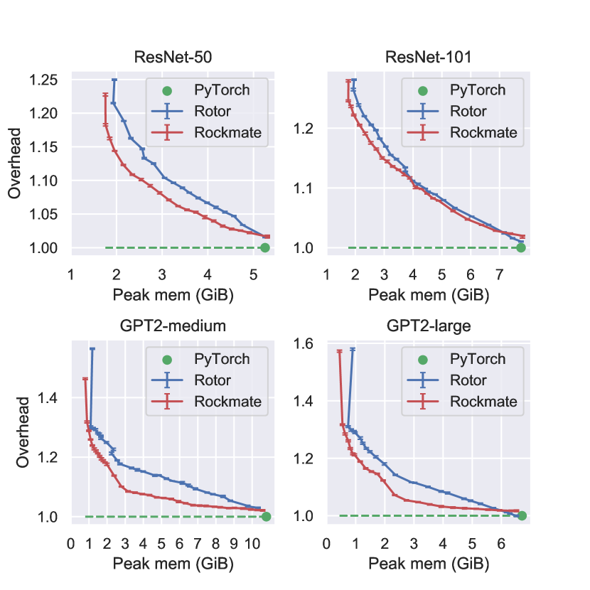
Figure 6: Computational overhead versus peak memory usage on different networks. Within the same memory usage, Rockmate is faster than Rotor in most cases. On GPT-like models, Rockmate significantly outperforms Rotor.

We compare Rockmate with Rotor on ResNet and GPT2 models over a range of memory budgets. Figure 6 shows the computational overhead in terms of peak memory usage during the forward-backward computations. For the same memory peak, Rockmate has a lower overhead than Rotor in most cases. For ResNet models, Rockmate does not show a significant improvement over Rotor, especially when the neural networks are deep enough, in which cases Rotor has more re-materialization options. On the other hand, Rockmate shows much better performance than Rotor on GPT2 networks. For GPT2-large it is noteworthy that Rockmate saves 50% memory by introducing only 5% overhead, while Rotor has more than 10% overhead for the same budget. In addition, Rockmate allows training with a smaller memory budget. To train GPT2-large, Rotor requires at least 720 MB memory budget, while Rockmate only requires 440 MB.

The reason why Rockmate significantly outperforms Rotor is that there are ”cheap” operations inside a Transformer block, such as dropout and gelu. The tensors generated by these operations consume a lot of memory, but there is almost no cost to recompute these operations. Because Rotor rematerializes one block at a time, it cannot take advantage of the ”cheap” operations to optimize performance. Rockmate works particularly well on models with a sequential-like structure, where each part contains a complicated structure.

While Rotor can only handle nn.Sequential-type models as input, Rockmate can be applied to more general types of neural networks. In Figure 7 we show the results of using Rockmate directly on the RegNet model imported directly from torchvision, whereas using it in Rotor would require to rewrite the code to highlight the sequential part. Although performance may vary depending on the structure of the neural networks, Rockmate can be used to save memory on general PyTorch models.

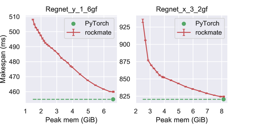
Figure 7: RegNet imported from torchvision is tested by Rockmate. Makespan is the time of one training iteration (including forward and backward).

5 Conclusion and Perspectives

In this paper, we propose Rockmate, a fully automatic tool that takes as input a PyTorch model in the form of a nn.Module and a memory limit for activations and automatically generates another nn.Module, perfectly equivalent from the numerical point of view, but that fulfills the memory limit for activations at the cost of a small computational overhead. Through experiments on various models, we show that the computation time of the resulting nn.Module is negligible in practice and that the computational overhead is acceptable, even for drastic reductions in memory footprint. Rockmate is therefore a tool that can transparently allow increasing model size, data resolution and batch size without having to upgrade GPUs. This work opens several new scientific questions. First, Rockmate is very efficient for graphs that can be written as a sequence of blocks, which corresponds to numerous models in practice but not to all of them, which raises the question of its extension to any type of graph. Then, the combination of Rockmate with data parallelism is trivial, but the question of finding a partition of the model adapted to model parallelism that balances well the computational load and the memory footprint on the different nodes is also an open problem.

Acknowledgements

This work has been partially funded by the Inria DFKI ENGAGE Project: nExt geNeration computinG environments for Artificial intelliGEnce.

Appendix A rk-GraphBuilder

A.1 Outline

We have developed the Rockmate Graph Builder (rk-GB) as a tool for producing the graphs required for Rockmate. Although it was developed for this specific purpose, it can also be used independently. Given a torch.nn.Module and a given input for that module, our goal is to generate a graph showing all the operations that occur during the forward and backward of the module on that given input. Having a specific input is important for both the resolution of if statements in the forward code and the inspection of each operation. Indeed, since our goal is to identify recomputations, we have to know the time spent and the memory footprint for each operation, that both depend on the input.

rk-GB relies on torch.jit.trace to trace the execution of the forward module on the input. This function runs the forward code and returns the list of all performed operations. Based on this list, we build the forward graph and transform it through several steps to generate what is needed by Rockmate. Note that currently rk-GB may fail due to limitations of torch.jit.trace, for instance it does not work properly on the GPT model from HuggingFace. However, PyTorch 2.0 was recently announced with a new way to capture graphs: TorchDynamo. According to its authors, TorchDynamo is expected to work with almost all modules. We plan to try changing from jit.trace to TorchDynamo.

rk-GB consists of five steps. First, we build the forward graph based on jit.trace, also collecting some information about each node. Then we simplify the graph. This part significantly reduces the number of nodes, which is a nice feature for the ILP used in rk-Checkmate. This is more than just an optimization, it’s a requirement for correct re-materialization. Next, we split the simplified forward graph into blocks using the 1-separator list. This produces a sequence of forward graphs, which we refer to as blocks. Rockmate will process each block with rk-Checkmate, and then process the whole chain with rk-Rotor. At this point, similar blocks are detected to avoid solving the same problem multiple times. Finally, for each unique forward block, we build the forward + backward graph and monitor the time and memory usage of each node during this step.

A.2 The forward graph

First, we call torch.jit.trace_module to get the forward code of any given torch.nn.Module. Specifically, we use the code_with_constants attribute of the output object, which is a code string of the assignments made during the forward phase. In Rockmate, a list of assignments is required, where each line consists of exactly one target and one operation.

Therefore,
a,b = torch.chunk(torch.relu(M),2)
becomes
fv_1 = torch.relu(M) ;
fv_2 = torch.chunk(fv_1,2) ;
a = fv_2[0] ; b = fv_2[1]

We also need to inline submodules code, so that
b = self.layer1(input) ;
output = self.layer2(b)
becomes
# layer1 part :
fv1 = torch.linear(input, ...) ;
fv2 = torch.relu(fv1) ;
fv3 = torch.linear(fv2, ...) ;
# layer2 part :
fv4 = torch.dropout(fv3,0.1)
output = torch.layer_norm(fv4,...)

We can access the code of the submodules through the object returned by jit.trace_module with :
<jit_output>.<submodule name>.code
We assign a unique number to each target to avoid name collisions when building the submodule code.

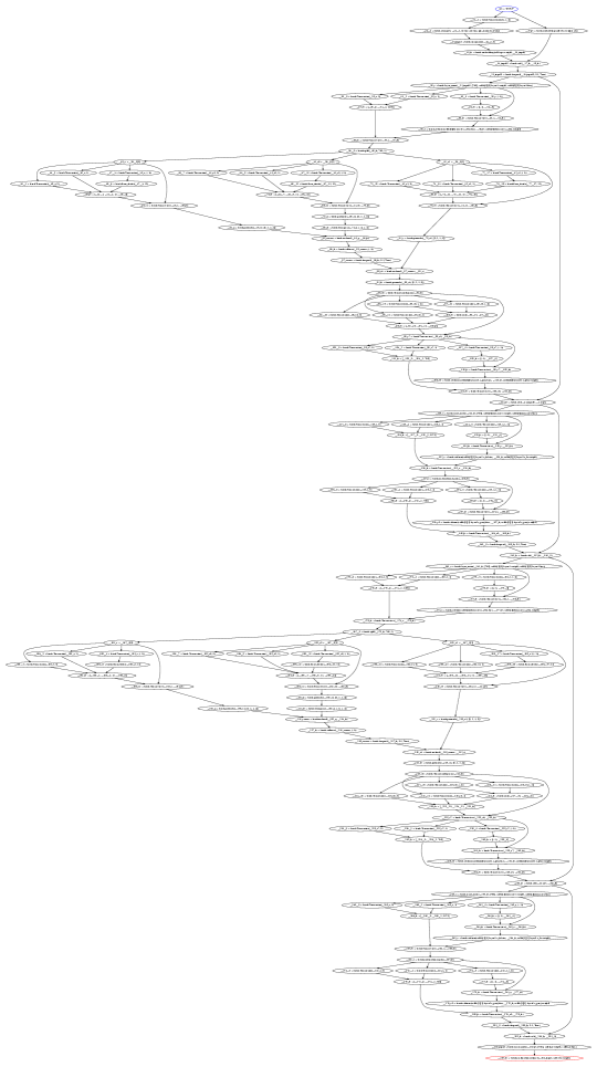
Figure 8: Forward graph of a GPT2 with 2 transformer blocks.
All the figures are generated using rk-GB print_graph function, which relies on Graphviz.

A.3 Simplification

In Rockmate, we want to perform both forward and backward operations on nodes, with the ability to delete and recompute tensors. Both view and in-place operations share their data with their input, so that deleting a node without also deleting its views is not allowed. All nodes related to the same data must be merged. After the simplification part, each node consists of exactly one primary allocation, which creates a data item, and some secondary allocations associated with that data, that do not allocate new memory.

First, we need to run each node to analyze it, since the name of the function might not be enough to determine whether the operation creates a new data item or not. For example, the function torch.contiguous may create a new data item depending on whether the input data is contiguously stored in memory or not. Another common example is torch.reshape, which is a visualization function if and only if the input and the requested shape have compatible strides. A robust way to check if two tensors refer to the same data is to compare their attribute data_ptr. To do this, we must create each variable, determine its type, and, if it is a tensor, check whether its data_ptr is new or not.

Analysis of each node

Note that we cannot analyze all of the code at once, as this would result in all intermediate activations being stored in memory, which is inconsistent with Rockmate’s goal of using as little memory as possible. We will analyze each node separately, without storing any tensor. We proceed as follows

• First, we randomly generate its inputs. Since we traverse the nodes in a topological order, the inputs have already been analyzed. For the reasons mentioned earlier, the tensors have not been stored, but their data type and shape have been recorded. Therefore, we can randomly generate the inputs based on this information. . For example, as mentioned earlier, the behavior of torch.reshape depends on whether the input and the required shape have compatible strides. Therefore, to generate the inputs correctly, we regenerate the data and perform all view operations on it before analyzing the node.

• Then we run the code to analyze, which consists of an assignment, so that we get a value. If it is a torch.Size (or something similar), we store it and mark it as a node of type size. Otherwise it consists of either a tensor or a list of tensors. In both cases it has a data_ptr. First we check if the value already exists in the local directory, in which case it is an in-place operation. Consider the following example:
  A = torch.linear(M,...) ;
  A += M
  It appears in the forward graph as
  A = torch.linear(M,...) ;
  fv1 = torch.Tensor.add_(A,M)
  When analyzing the node of fv1, we must recognize that it is the result of an in-place operation on A. In this case, fv1 refers to the same Python object as A. So to detect an in-place operation, we compare the address of the object fv1 with its inputs (using the Python keyword is). If we find a match, we mark the node as in-place and record the name of its data owner (in the example above, the data owner of fv1 is A). Otherwise, we check if the value shares its data_ptr with one of its inputs, in which case it is a node of type view, and we record the name of its data owner. Finally, by default, the tensor is an original data and its data owner is itself. We call this case by default the operation real.

• Finally, we store information such as the type and shape of the data so that we can randomly regenerate data when analyzing upcoming nodes. Note that we also need to store the requires_grad information. It is essential for building the backward graph, and we need to use it when regenerating tensors.

Simplification process

Once the analysis has been performed, the simplification of the graph can be started. The simplification is done in three steps:

• First, we process so-called cheap operations, such as list and tuple constructors. In contrast to the following simplification steps, here we insert the code to be simplified directly into the user code, for example
  fv1 = [s1,s2] ;
  B = torch.reshape(A,fv1)
  becomes
  B = torch.reshape(A, [s1,s2])
  Simplifying the list and tuple constructors is mandatory to ensure each node represents only one tensor, it also makes the code easier to read. cheap operations also include torch.add, sub, mul, and div. This is due to the way autograd handles intermediate results. Normally, nested operations (neither primary nor inline) create intermediate variables that are stored in grad_fn. Therefore, we repeat the submodules until we reach primary operations. But these specific operations do not create intermediate data in grad_fn (because we do not need them during backward). Therefore, it is preferable not to inline them, as otherwise they would explicitly create intermediate variables and thus use more memory. Note that we could duplicate the code:
  A = torch.add(B, C) ;
  D = torch.linear(A,...) ;
  E = torch.relu(A)
  becomes
  D = torch.linear(
  D = torchtorch.add(B, C),...) ;
  E = torch.relu(torch.add(B, C))
  Since these operations are fast enough (e.g. compared to torch.matmul), it will not take too much time. However, these simplifications represent a trade-off between the number of intermediate variables and the number of dependencies. In the example above, D now depends on both B and C. Therefore, it is optional to consider Add, Sub, Mul and Div as cheap operations.

• The second step in the simplification process concerns nodes of type size. Since these operations do not create data, we move them as secondary assignments of the node they refer to, which we call the body_code. To avoid creating new dependencies, for example in the case where a node depends only on the shape of a tensor and not on the tensor itself:
  s = torch.Tensor.size(A,0) ;
  ...
  C = torch.reshape(B, [s])
  

  In this example, we are not yet sure whether C depends directly on A, but merging s into A would actually enforce the dependency. That would be wrong because it would cause Rockmate to conclude that A cannot be forgotten before computing C. To avoid this, even though the assignment of s is inserted into the body code of A, we do not delete the node of s, but simply mark it as artifact. Artifacts are nodes concerning size-type operations that are needed to avoid creating dependencies between real nodes. After each simplification, we perform a test to determine if any of the artifact nodes can be removed. In the example above, if it turns out that B is a view of A, in the third simplification step, the assignment of B is moved to the body code of A, after which C depends directly on the node of A, so we can remove the artifact node of s.

• Finally, the view and insert operations are simplified. View nodes are merged with the node of their data owner by inserting their assignment into the body code of the data owner. The same idea applies to in-place operations, i.e. we insert them into the node of their data owner. However, since Rockmate wants to control the backward execution, after each main operation we detach the tensor to split the backward graph. This detach operation must be performed before creating different independent views, otherwise we would have to detach each view independently, which is impossible in PyTorch. On the other hand, the detach operation must be performed after in-place operations because they impact the data, even though these in-place operations can be applied to views and not directly to the original tensor. PyTorch is aware of that, so it ensures it’s impossible to have in-place operations over different independent views, therefore we always have a valid way to run the code and detach at the right position. An attribute in-place_code is provided to handle the detach operation.

Artifact nodes which survived until the end of simplification will be considered as soft-dependencies when at the moment we generate a topological order for the final forward-backward graph, only to ensure the owner of an artifact always comes before any of its users. Apart from that they are removed. Thus, we do not create explicit dependencies, but since ILP follows the topological order for the first computation of each node, the size information is computed before it is used and is not forgotten.

At the end of the simplification, we end up with a forward graph, where each node consists of exactly one real operation that creates a data, and some secondary operations on it. As for the topological order, we follow the original order by using the unique number we assigned to each variable. Thus, we keep the order in which jit performed the forward code of the original module. Finally, although we will not discuss it in detail, we also handle random operations.

Figure 9: Number of nodes in the basic forward graph compared to the simplified one.

	Basic graph	Simplified graph
GPT2(nlayers=2)	164	35
Resnet101	346	211
Regnet_x_32gf	245	173
MLP Mixer	203	124
nn.Transformer	161	51

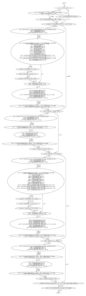
Figure 10: Simplified forward graph of a GPT2 with 2 transformer blocks, generated by PGB.

A.4 Cut the forward graph

The subsequent steps of Rockmate rely on a list of blocks in order to apply rk-Checkmate to each block independently. We cut the simplified forward graph into a sequence of blocks. The cuts are made along the 1-separators of the graph: these are nodes whose removal result in a disconnected graph. We obtain the list of separators by using a variant of Breadth First Search (BFS). Note that although we cut the simplified graph, a first draft of the separators list is computed before we perform the simplifications. We mark potential separators as protected to avoid oversimplifying the graph, which could break its overall structure. Since torch.add operations are simplified by default, without this protection, all residual edges would traverse the entire graph from input directly to output. As a result, the simplified graph would consist of a single large block with many undesirable dependencies. The protected nodes, which are potential separators, bypass the cheap simplification step. At the end of the simplification step, the list of separators is recomputed, as it may have changed due to other simplifications.

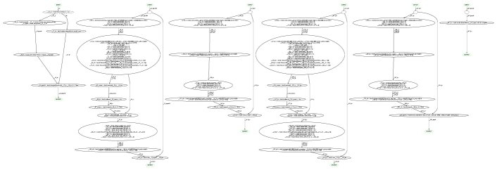
Figure 11: Cut simplified forward graph of a GPT2 with 2 transformer blocks, generated by PGB.

A.5 Recognition of Similar Blocks

To reduce solving time, we would like to avoid solving the same ILP multiple times on identical blocks. For example, GPT2 consists of $n$ attention blocks interleaved with $n$ feedforward blocks, and the resolution of this ILP $n$ times on identical instances should be avoided. We developed a tool to generate classes of identical blocks.

• First, we provide a function to anonymize simplified graphs. Given a simplified graph, we build a parser that maps all target names to numbers starting with 1 and also anonymizes the parameter names.

• To test if two blocks are identical, we compare their anonymized versions. This is done by visiting each node in turn, following some topological order (which should be the same if the blocks are identical). For each pair of nodes, we compare their attributes: the code, but also the information about each variable, including its type and shape. The lists of parameters should also have the same anonymized names (i.e. they are used in the same nodes), but also the same data types and shapes.

• After building the equivalence classes, we directly build the forward+backward graph for each unique anonymous graph, and translate it back to un-anonymize and get the forward+backward of each block. In Rockmate, we solve the ILP once for each equivalence class, and the resulting R and S matrices can be shared across identical blocks.

Figure 12: Total number of blocks in the cut simplified graph compared to the number of unique blocks.

	Chain length	Unique blocks
GPT2	nlayers$>1$	5
Resnet101	38	13
Regnet_x_32gf	27	11
MLP Mixer	27	6
nn.Transformer	3	3

In the GPT2 implementation used in the experiments, there are only five unique blocks. Each transformer layer is automatically divided into two blocks, corresponding to a attention part and a MLP part. The five unique blocks are: the input pre-processing, a typical attention block, a typical MLP block, the last MLP block which is slightly different due to simplification, and the final output post-processing. Therefore, regardless of the number of transformer blocks, the overall solving time for rk-Checkmate is constant.

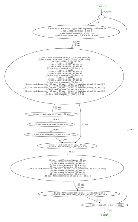
Figure 13: An anonymized version of an attention block from GPT2

A.6 Inspection and backward nodes

Since we now have exactly one data defined per node, we can associate one backward operation with each forward node, whose code is given by _<target>.backward(<target>.grad)

In rk-Checkmate two categories of nodes are introduced: Computation nodes (C_nodes) and Data nodes (D_nodes). A C_node represents an operation that takes a certain amount of time to execute with a certain amount of memory overhead. It is either a Forward or a Backward node. A D_node represents an item stored in memory. D_nodes can be deleted to free memory, and C_nodes can be recomputed to restore D_nodes, although it takes some time. . There are three types of D_nodes: tensor.data attribute, tensor.grad attribute, and what we call phantoms, which are intermediate results (saved_tensors) stored in the grad_fn attribute.

We consider each node of the simplified forward graph one at a time in topological order. To create the C and D_nodes we need to do an inspection, i.e. to run the code several times to measure time and memory usage. First we run the forward code (including the body part) and measure how much memory has been allocated, then we set the .data attribute to torch.empty(0) to free the memory.

The memory successfully freed is the memory used by the tensor.data’s D_node. If some memory was not freed, it means that the node has phantoms. Phantoms are intermediate values stored in tensor.grad_fn in preparation for backward.

To handle phantoms properly, we handle any ._saved_tensors or .variable attributes. We use the grad_fn.next_functions attribute to recursively open the grad_fn graph. The .variable attribute is an explicit reference to a variable (e.g. the input of the forward operation), while _saved_tensors are either views of known tensors or original tensors. The opening of grad_fn is crucial for three reasons:

• First, we need to open grad_fn to properly build backward C_nodes dependencies. Indeed, an input of the forward operation is needed to perform the backward operation if and only if there is a reference to it in the grad_fn. Consider a first example: B = torch.addmm(bias,A,weight)
  In such a case, A.data is indeed necessary to run B.backward and a reference to it can be found in B.grad_fn. Therefore, B’s backward C_node depends on A’s data D_node. Now consider a second example:
  C = torch.add(A,B)

  Here, given C.grad, both A.grad and B.grad can be computed without A.data or B.data, so that we do not want backward C_node of C to depend on A and B’s data D_nodes. Note that autograd always checks the shape of the .data attribute of inputs, even if they are not used. To solve this problem, we introduce two types of dependencies (i.e. edges of the graph): actual and fake. fake edges do not appear in the ILP, we do not want to force the data to be alive if it is not used. fake edges are only used in Rockmate’s final code generator: in the example above, C’s backward fakely depends on A and B’s data, so by the time we want to run C’s backward, A.data may already be forgotten. To pass the autograd shape equality check, we need to assign an empty tensor with the correct shape to A.data. To avoid wasting memory for this, we use A.data = torch.ones(1)
  A.data = torc .expand(<numel(A)>)
  A.data = torc .view(<shape(a)>)
  

  Using this trick we allocate only 512 octets, whereas: A.data = torch.empty(<shape(a)>)
  would allocate as much memory as the original A.data and cancel our efforts to let the solver free A’s data to reduce memory footprint.

• In the previous paragraph we explained the user’s viewpoint: given a tensor, we want to find its dependencies. Let us now take the input perspective. If a _saved_tensor is a view of the input, it means that input.data = torch.empty(0) will not free anything. To free a data we must put the data attribute of all the tensors having the same data_ptr to torch.empty(0), including the _saved_tensors which refer to it. The correct way to forget a data is therefore input.data = torch.empty(0) ;
  input_view.data = torch.empty(0) ;
  user.grad_fn.next_functions[0][0]._saved_mat1.data= torch.empty(0)

  Similarly, after recomputing input’s data, all _saved_tensors that refer to it are rebuilt. Even if it is not directly the same data, but a view of it, we take care to rebuild it properly, including operations that affect the strides. autograd can store any view of the data, but there is no way to guess if the stride will be affected. However, we use all known views of the data that are not phantoms, and we find one that is compatible with the _saved_tensor. Therefore, for a node, we need the names of the phantoms that are views of it.

• As mentioned before, phantoms can be either references to existing tensors or original tensors. If original tensors are found in grad_fn, there will be a difference between the memory generated during forward and the memory freed when forgetting .data. In this case we create a phantom D_node. This node has exactly one dependency (to the forward C_node) and one user (the backward C_node).

By inspecting forward execution and backward when requires_grad is set, we obtain the memory and time attributes of all the mentioned nodes. Finally, there is another special C_node . It applies to everything related to loss. The special loss C_node depends on the model’s output data D_node and is required by the model’s output grad D_node. This node has no code attribute, it is a placeholder to split the final schedule into forward and backward phases. In the rk-Checkmate generated schedule, the backward part starts as soon as this C_node is computed. Furthermore, in rk-Checkmate’s ILP, in addition to the generation constraint: $memory\_allocated<M_{peak}$, we can control that at the moment when the special loss_node is computed, $memory\_allocated<M_{save}$.

Let us conclude with two final remarks

• In addition to actual and fake edges, we introduce global edges. For example, the first C_nodes of a block global depend on the data D_node of the previous block. These edges assist the final code generator. Using these edges, we have the entire forward +backward graph.

• Measuring GPU memory usage with cuda is accurate, but running the same operation twice in different contexts can result in different amounts of memory being allocated. Therefore, the final execution may allocate more or less memory than we predicted. This is due to the way cuda allocates memory, trying to minimize memory fragmentation. But it’s usually very small.

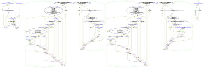
Figure 14: Final product of rk-GB for a GPT2 with 2 transformer blocks.
Forward C_nodes are in blue, backward ones in violet, D_nodes in gold, special nodes in green.

Appendix B rk-Checkmate: ILP details

B.1 Graph and objective

As it was discussed in section 3.3, at block level we find an optimal re-materialization strategy given memory budget via proposed rk-Checkmate algorithm.

Note that in Checkmate paper, they assume only one output is generated from each operation across the forward and backward graph. In PyTorch, such an assumption is not feasible in general cases: tensor.grad_fn tends to generate the gradients of all relevant input tensors. Therefore, our rk-Checkmate is based on a graph where each computation node can produce multiple data nodes. Moreover, if tensor is used in computation of different target’s, tensor.grad may be generated in any backward node of target.

Input to the rk-Checkmate is a CD_graph built by rk-GB. CD_graph is a directed acyclic graph, which containts:

• $D$ data nodes $\{v_{1},\dots,v_{D}\}$ and $T$ computational nodes $\{w_{1},\dots,w_{T}\}$,

• edges of type $v_{d}\rightarrow w_{t}$ and $w_{t}\rightarrow v_{d}$ that show dependencies between computational operations and data. For example, $v_{d}$ is used to perform computation $w_{t}$, and computation $w_{t}$ outputs data $v_{d}$ as a result. One computational node can have several incoming data nodes and vice versa.

To find an optimal re-materialization strategy for one block given memory budget and computation-data dependencies described with CD_graph, we solve an integer linear programming (ILP) problem, which minimizes computational costs required for propagation through the block given feasibility and memory constraints.

Denote by $stage_{t-1\rightarrow t}$ a period, which starts after the result of computation $w_{t-1}$ is obtained for the first time and ends when the computation $w_{t}$ is firstly performed. During one stage several computations from $\{w_{t^{\prime}}\}_{t^{\prime}\leq t}$ and deletions might happen.

The solution of ILP provides a schedule $\mathbf{R}$ (low-triangular binary matrix $T\times T$) that determines which computations should be performed during each stage.

$$R_{t,t^{\prime}}=\begin{cases}1,\quad\text{if we compute $w_{t^{\prime}}$ during the $stage_{t-1\rightarrow t}$}\\ 0,\quad\text{otherwise}\end{cases}\,.$$

Each stage can be seen as a sequence of steps, such that during one $step_{t^{\prime}-1\rightarrow t^{\prime}}$ one computation $w_{t^{\prime}}$ is done (or not if the schedule doesn’t require that, i.e. if $R_{t,t^{\prime}}=0$) and some tensors are deleted.

Also, the solution of ILP provides an information $\mathbf{S}$ about data nodes saved during each stage.

$$S_{t,(t^{\prime},d)}=\begin{cases}1,\quad\text{if during $stage_{t-1\rightarrow t}$ an output data tensor $v_{d}$ of computation $w_{t^{\prime}}$ is saved}\\ 0,\quad\text{otherwise}\end{cases}\,.$$

Consider all edges in CD_graph that connect computation nodes with their children data nodes,

$${ChildrenOfComp:=\{(t^{\prime},d)|\ v_{d}\in children(w_{t^{\prime}}),t^{\prime}=1,\dots,T\}},$$

and let their number equals $|ChildrenOfComp|=E^{t\rightarrow d}$. Then $S$ can be seen as binary matrix of size $T\times E^{t\rightarrow d}$.

Thus, given memory budget, ILP finds schedule $R,S$ such that computational costs

$$\sum_{1\leq t^{\prime}<t\leq T}C_{t^{\prime}}R_{t,t^{\prime}}$$

are minimized given feasibility and memory constraints (where $C_{t^{\prime}}$ is a cost of computation $w_{t^{\prime}}$). Now let us take a closer look to the constraints.

B.2 Feasibility constraints

Consider all edges in CD_graph that connect data nodes with their parent computation nodes

$$ParentsOfData:=\{(t^{\prime},d)|\ w_{t^{\prime}}\in parents(v_{d}),d=1,\dots,D\}$$

$$ChildrenOfData:=\{(t^{\prime},d)|\ w_{t^{\prime}}\in children(v_{d}),d=1,\dots,D\}$$

then a set of edges, which connects each data node with its children and parent computation nodes, can be expressed as

$${ChildrenParentsOfData:=ChildrenOfData\cup ParentsOfData}$$

and let their number equals $|ChildrenParentsOfData|=E^{t\rightarrow d\rightarrow t}$.

Let also introduce a binary matrix $P$ of size $T\times D$, where

$$P_{t,d}=\begin{cases}1,\quad\text{if we have data tensor $v_{d}$ in memory after the end of $stage_{t-1\rightarrow t}$}\\ 0,\quad\text{otherwise}\end{cases}\,.$$

Note that $P_{t,d}\geq S_{t,(t^{\prime},d)}/|parents(v_{d})|$.

The following constraints for ILP should be hold

• $\sum\limits_{t=1}^{T}\sum\limits_{t^{\prime}=t+1}^{T}R_{t,t^{\prime}}=0$: ensures that we can recompute only operations that have been executed during previous stages.

• $\sum\limits_{e}\sum\limits_{t=1}^{t^{\prime\prime}-1}S_{t,e}=0$, where $e=(t^{\prime\prime},d),e\in ChildrenOfComp$: ensures that before the first computation, data cannot be saved.

• $\sum\limits_{d=1}^{D}\sum\limits_{t=1}^{t^{\prime}}P_{t,d}=0,$ where $t^{\prime}=\min\{t^{\prime\prime}|w_{t^{\prime\prime}}\in parents(v_{d})\}$: ensures data tensor $v_{d}$ isn’t stored before the execution of first coputation that contributes to its value.

• $\sum\limits_{t=1}^{T}R_{t,t}=T$: ensures that $w_{t}$ is executed at the end of $stage_{t-1->t}$.

• $\sum\limits_{t=1}^{T}R_{t,t_{loss}}=1,$ where $t_{loss}$ is an index of node that computes the loss: ensures that the loss is computed only once during the forward-backward phase.

• $S_{t,e}\leq P_{t,d},$ where $e=(t^{\prime},d)\in ChildrenOfComp$ and $t,t^{\prime}=1,\dots,T$

• $S_{t+1,e}\leq S_{t,e}+R_{t,t^{\prime}},$ where $e=(t^{\prime},d)\in ChildrenOfComp$ and $t=1,\dots,T-1$

• $R_{t,t^{\prime}}\leq R_{t,t^{\prime\prime}}+S_{t,e},$ where $t^{\prime}\in children(d),e=(t^{\prime\prime},d),e\in ChildrenOfComp$, and $t=1,\dots T$: ensures that all computations $w_{t^{\prime}}$ which are required for generation of data $v_{d}$ are present, where $v_{d}$ is an input data for computation $w_{t}$.

B.3 Memory constraints

Let $ChildrenOfData[d]$ denotes a set of indices of computation nodes $w_{t}$, which requires tensor $d$.

And let $ParentsOfData[d]$ returns a set of indices of computation nodes $w_{t}$, which generates tensor $d$.

We remind that each stage can be seen as a sequence of steps, such that during one step one computation (or not if the schedule doesn’t require that) and some tensors are deleted.

To represent the presence of certain tensors at different steps $step_{t^{\prime}-1\rightarrow t^{\prime}}$ of each stage $stage_{t-1\rightarrow t}$, we introduce the following variables:

$create_{t,d,t^{\prime}}\in\{0,1\},\forall t^{\prime}\in ParentsOfData[d]$: whether tensor $v_{d}$ is created during $step_{t^{\prime}-1\rightarrow t^{\prime}}$ at stage $stage_{t-1\rightarrow t}$.

$delete_{t,d,t^{\prime}}\in\{0,1\},\forall t^{\prime}\in(ParentsOfData[d]+ChildrenOfData[d])$: whether tensor $d$ is deleted during $step_{t^{\prime}-1\rightarrow t^{\prime}}$ at stage $stage_{t-1\rightarrow t}$.

Let us define expression for $t=1,\dots,T$ and $(t^{\prime},d)\in ChildrenParentsOfData$:

$$alive[t,d,t^{\prime}]=P_{t,d}+\sum_{t^{\prime\prime}\leq t^{\prime}}create_{t,d,t^{\prime\prime}}-\sum_{t^{\prime\prime}\leq t^{\prime}}delete_{t,d,t^{\prime\prime}}\in\{0,1\}.$$

A tensor $v_{d}$ is either alive or deleted immediately after the computation of parent nodes:

$$alive[t,d,t^{\prime}]+delete_{t,d,t^{\prime}}\geq R_{t,t^{\prime}},$$

A tensor $v_{d}$ is retained during $stage_{t-1\rightarrow t}$ if it is alive during the last posssible step of $stage_{t-2\rightarrow t-1}$:

$$alive[t,d,t^{\prime}]=P_{t,d},t^{\prime}=max(ParentsOfData[d],ChildrenOfData[d])$$

A tensor can only be created from the parent computation:

$$create_{t,d,t^{\prime}}\leq R_{t,t^{\prime}}$$

A tensor should be deleted if it would not be needed or saved in the current stage:

$$delete_{t,d,t^{\prime}}=R_{t,t^{\prime}}*\prod_{d^{\prime}\in att(d)}(1-P_{t+1,d^{\prime}})*\prod_{t^{\prime\prime}\in children(v_{d})|t^{\prime\prime}>t^{\prime}}(1-R_{t,t^{\prime\prime}})$$

No tensor should be alive after the final stage:

$$alive[T,d,t^{\prime}]=0,\ t^{\prime}=max(ParentsOfData[d]+ChildrenOfData[d])$$

‘’ Let $U_{t,t^{\prime}}$ denotes the memory saved at the end of $step_{t^{\prime}-1\rightarrow t^{\prime}}$ during $stage_{t-1\rightarrow t}$ and $M_{d}$ is the memory required to store tensor $v_{d}$, then

$$U_{t,1}=\sum_{d=1}^{D}M_{d}P_{t,d}+\sum_{d=1}^{D}{M_{d}\ create_{t,d,1}}-\sum_{d=1}^{D}{M_{d}\ delete_{t,d,1}}$$

$$U_{t,t^{\prime}}=U_{t,t^{\prime}-1}+\sum_{d=1}^{D}{M_{d}\ create_{t,d,t^{\prime}}}-\sum_{d=1}^{D}{M_{d}\ delete_{t,d,t^{\prime}}}$$

The peak memory at $step_{t^{\prime}-1\rightarrow t^{\prime}}$ during $stage_{t-1\rightarrow t}$ is within memory budget:

$$tmpM_{t^{\prime}}R_{t,t^{\prime}}+U_{t,t^{\prime}}+\sum_{\forall i}{M_{d}delete_{t,d,t^{\prime}}}\leq M_{budget}$$

where $tmpM_{t^{\prime}}$ is the temporary memory overhead needed in the computation node $w_{t^{\prime}}$.

Appendix C rk-Rotor

C.1 Notations

Assume our model is a sequence of $L$ blocks, numbered from $0$ to $L-1$. For each block, we have $1+B$ budget options, where option $0$ does not save any intermediate data, and each of the other $B$ options saves a different amount of data. We denote by $F_{i}^{o}$ the forward computation of block $i$ with option $o$, and if $o>0$, $B_{i}^{o}$ is the corresponding backward computation. Since $F_{i}^{0}$ does not store any intermediate data, we consider that it does not have a corresponding backward computation.

The input activation of $F_{i}$ is $x_{i}$, and its output is $x_{i+1}$. Similar to the Rotor paper (Beaumont et al., 2019b), for each option $o>0$, we denote by $\bar{x}_{i}^{o}$ the union of $x_{i}$ and of all the intermediate data generated by $F_{i}^{o}$. For ease of notation, we will also use $x_{i}$ and $\bar{x}_{i}^{o}$ to denote the size of the corresponding data.

For any computation, we use $tmp(\cdot)$ to denote the temporary memory usage of this computation: this is the amount of memory that needs to be available for this computation to succeed, and that is released afterwards. We also use $r(\cdot)$ to denote the running time of an computation. As an example, since the input and output data need to be in memory, the memory usage for running $F_{i}^{0}$ is $x_{i}+x_{i+1}+tmp(F_{i}^{0})$, and this takes time $r(F_{i}^{0})$.

C.2 Formulation

We denote by $\text{Opt}(s,t,m)$ the optimal execution time for computing the sequence from block $s$ to block $t$, assuming that the input $x_{s}$ will be kept in memory. There are two possible cases for the start of this computation:

• If block $s$ is only computed once in this sequence, then it is computed with one of the $F_{i}^{o}$ options for $o>0$ so that it is possible to perform the backward computation. This requires to have at least $tmp(F_{i}^{o})$ available memory for the forward and at least $tmp(B_{i}^{o})$ available for the backward. The corresponding execution time is $r(F_{i}^{o})+r(B_{i}^{o})$, and the memory available for the rest of the computation is $m-\bar{x}_{i}^{o}$. The best choice is given by:

  $$\text{Opt}_{1}(s,t,m)=\min_{\text{valid option $o$}}r(F_{i}^{o})+r(B_{i}^{o})+\text{Opt}(s,t,m-\bar{x}_{i}^{o})$$ (1)

  In this equation, an option is considered valid if the temporary memory requirements for the forward and backward computations are satisfied.

• If block $s$ is computed more than once, then its first computation does not need to keep any intermediate data. It is thus computed with $F_{s}^{0}$, and the choice now is about which is the next activation to be kept in memory. Let us denote by $i$ the index activation kept in memory, so that activations $x_{s+1},x_{s+2},\dots,x_{i-1}$ are discarded just after being used. It is possible to compute $x_{i}$ by performing $F_{s}^{0},F_{s+1}^{0},\dots,F_{i-1}^{0}$. Once this activation is computed and stored in memory, optimizing the rest of the computation becomes a subproblem: we need to compute the optimal execution time from block $i$ to $t$. Afterwards, since no activation was stored between blocks $s$ and $i$, this corresponds to another subproblem, from $s$ to $i$. The best choice is given by:

  $$\text{Opt}_{2}(s,t,m)=\min_{\text{valid choice $i$ with $s<i<t$}}r(F_{s}^{0})+r(F_{s+1}^{0})+\cdots+r(F_{i-1}^{0})+\text{Opt}(i,t,m-x_{i})+\text{Opt}(s,i,m)$$ (2)

  In this equation, a choice is considered valid if the temporary memory requirements for all computations $F_{s}^{0},F_{s+1}^{0},\dots,F_{i-1}^{0}$ are satisfied.

In both cases, if there is no valid choice, the corresponding $\min$ value is considered to be $+\infty$. Finally, the optimal decision for our problem is computed with:

$$\text{Opt}(s,t,m)=\min\big{(}\text{Opt}_{1}(s,t,m),\text{Opt}_{2}(s,t,m)\big{)}$$ (3)

Additionally, if $s=t+1$, only the first case can be considered, but this time the rest of the computation is empty. We can thus compute $\text{Opt}(s,s+1,m)$ for all $s$ and all $m$. The resulting algorithm is close to the Rotor algorithm, using the updated equation (1), and is provided in Algorithm 2.

Algorithm 2 rk-Rotor for $L$ blocks with memory $m$.

1:  for $m=1,\dots,M$ do

2:     for $k=1,\dots,L$ do

3:        for $s=1,\dots,L+1-d$ do

4:           Compute $\text{Opt}(s,s+k,m)$ with equation (3)

5:        end for

6:     end for

7:  end for

8:  return $\text{rk-Rotor-Build}(\text{Opt},1,L+1,m-x_{0})$ {Alg. 3}

Algorithm 3 $\text{rk-Rotor-Build}(\text{Opt},s,t,m)$ – Computation of the schedule

  if $\text{Opt}(s,t,m)=\infty$ then

     return Infeasible

  else if $s=t+1$ and $\text{Opt}(s,t,m)=\text{Opt}_{1}(s,t,m)$ with option $o$ then

     return $(F_{s}^{o},B_{s}^{o})$

  else if $\text{Opt}(s,t,m)=\text{Opt}_{2}(s,t,m)$ with choice $i$ (equation (2)) then

     return $(F_{s}^{0},F_{s+1}^{0},\dots,F_{i-1}^{0},\text{rk-Rotor-Build}(\text{Opt},i,t,m-x_{i}),\text{rk-Rotor-Build}(\text{Opt},s,i,m))$

  else

     $o\leftarrow$ option such that $\text{Opt}(s,t,m)=\text{Opt}_{1}(s,t,m)$ (equation (1))

     return $(F_{s}^{o},\text{rk-Rotor-Build}(\text{Opt},s+1,t,m-\bar{x}_{s}^{o}),B_{s}^{o})$

  end if

Appendix D rk-Exec

Rockmate’s final re-materialization schedule is a list of operations, either compute or forget. rk-Exec takes care of executing this schedule properly. It creates a new nn.Module that produces exactly the same results (both data and gradients) while respecting the requested budget. The schedule given to rk-Exec refers to C_nodes and D_nodes.

D.1 Computation

Remember that a C_node consists of a main assignment that creates the .data, and a body_code that contains secondary statements about shapes, views, and in-place operations. By default in PyTorch, during forward execution, autograd puts in output’s grad_fn all the information needed to go back directly from the loss to input’s gradients. The principle of memory saving is to control the backward and how intermediate activations are saved. To prevent autograd from creating the whole computational graph in output’s grad_fn, rk-Exec detach each tensor after computing it, so that grad_fn only keeps track of the last operation. Consider the following example

a = torch.linear(input,...) ;
b = torch.relu(a) ;
c = b.view(...) ;
d = torch.linear(c,...) ;
d.relu(inplace=True) ;
e = d.view(...)
output = torch.add(c,e) ;
For the forward we have :

• For C_node a
  _a = torch.linear(input,...) ;
  a = _a.detach().requires_grad_() ;

• For C_node b, viewing operations are done after detach
  _b = torch.relu(a) ;
  b = _b.detach().requires_grad_() ;
  c = torch.Tensor.view(b,...)

• For C_node d, in-place operations are done before detach
  _d = torch.linear(c) ;
  _fv1 = torch.relu_(_d) ;
  d = _d.detach().requires_grad_() ;
  fv1 = d ;
  e = torch.Tensor.view(fv1,...)

• For C_node output
  output = torch.add(c,e)

We always name with an underscore the variable before detaching, we call it the proxy. Based on this the backward computation is:
_<var_name>.backward(<var_name>.grad)

D.2 Deletions

Remember that there are three types of D_nodes:

• To free a tensor.data, we assign all views that refer to it to torch.empty(0). In the example above, to free d’s data D_node we set d.data, fv1.data and e.data to 0. But as mentioned in the rk-GB appendix, this also includes views that are stored in users’ grad_fn as _saved_tensors. For example, to free b’s data D_node you must perform
  _d.grad_fn.next_functions[0][0]._saved_mat1 = torch.empty(0)

• To free a phantoms D_node we just need to perform
  del _<var_name>
  It will delete the grad_fn, but the variable defined by the detach operation (<var_name>, without the underscore) will keep the tensor.data alive. So we just forget about the phantoms.

• To release a grad D_node, all we need is
  <var_name>.grad = None

D.3 Recomputation

To recompute a C_node rk-Exec reassign the proxy, but we do not detach again. Since the variable post-detach could be mentioned directly in its user grad_fn. We simply reassign the data attribute. In the example above, to recompute C_node we do:
_d = torch.linear(c) ;
_fv1 = torch.relu_(_d) ;
d.data = _d.data ;
fv1.data = d.data ;
e.data = torch.Tensor.view(fv1,...)
Furthermore, since re-materialization is the opposite of forgetting, we need to reassign the data attribute of all views, including the _saved_tensors that refer to them. Recomputing the phantoms and grad is trivial.

Last issues

• In the graph produced by rk-GB we introduced the notion of real and fake dependencies, they imply several tricks in rk-Exec. See the last part of the rk-GB appendix for explanations.

• To generate the code correctly, we compile the list of operations described in the schedule. That is, we generate the code one by one, but we keep track of which tensors are alive to avoid any if statements if the final code. For example, when we need to reassign all the views of a tensor in users grad_fn, we know which users are alive.

• Rockmate manipulates code that are either string or Python AST object we can execute. Therefore, rk-Exec generate a list of strings to execute. Then we can generate a big string code for the forward, and one for the backward, finally we use Python compile function to execute these functions without wasting time on parsing the string.

• We take care of random operations, in particular to be able to recompute a random function deterministically, we store random states on the first computation and restore them when needed.

• Note that sometimes, due to the float approximation precision, the results obtained from the original module and the new one may be a little different. But they are as close as running the original module twice. With torch.float64 precision there are always strictly equal on the model we tested.

Appendix E Detailed experiments on GPT2

Model	Input size	Algorithm	Budget (GiB)	Peak mem	Makespan	Makespan
				(GiB)	mean (ms)	std (ms)
GPT2-large	(2, 512)	PyTorch	$M_{GPU}$	6.708	457.173	1.207
GPT2-large	(2, 512)	Rotor	0.850	0.846	593.507	1.789
GPT2-large	(2, 512)	Rockmate	0.850	0.816	564.041	1.378
GPT2-large	(2, 512)	Rotor	2.800	2.360	522.163	0.889
GPT2-large	(2, 512)	Rockmate	2.800	2.741	481.650	0.992
GPT2-large	(2, 512)	Rotor	7.600	6.515	456.971	1.255
GPT2-large	(2, 512)	Rockmate	7.600	6.516	465.376	0.985
GPT2-large	(4, 256)	PyTorch	$M_{GPU}$	5.158	432.646	1.207
GPT2-large	(4, 256)	Rotor	0.850	0.808	561.066	1.791
GPT2-large	(4, 256)	Rockmate	0.850	0.795	531.255	0.732
GPT2-large	(4, 256)	Rotor	1.800	1.473	526.807	1.402
GPT2-large	(4, 256)	Rockmate	1.800	1.745	486.976	1.305
GPT2-large	(4, 256)	Rotor	5.600	4.690	439.797	1.451
GPT2-large	(4, 256)	Rockmate	5.600	4.967	440.410	1.469
GPT2-medium	(2, 1024)	PyTorch	$M_{GPU}$	10.782	480.330	0.975
GPT2-medium	(2, 1024)	Rotor	1.000	1.188	751.478	1.070
GPT2-medium	(2, 1024)	Rockmate	1.000	0.994	619.055	1.012
GPT2-medium	(2, 1024)	Rotor	4.000	3.351	558.858	1.208
GPT2-medium	(2, 1024)	Rockmate	4.000	3.941	516.758	0.899
GPT2-medium	(2, 1024)	Rotor	11.600	10.326	494.043	1.097
GPT2-medium	(2, 1024)	Rockmate	11.600	10.582	490.490	0.924
GPT2-medium	(4, 512)	PyTorch	$M_{GPU}$	7.407	430.596	1.206
GPT2-medium	(4, 512)	Rotor	1.000	1.188	658.736	1.105
GPT2-medium	(4, 512)	Rockmate	1.000	0.986	547.343	0.873
GPT2-medium	(4, 512)	Rotor	2.000	1.824	532.637	1.686
GPT2-medium	(4, 512)	Rockmate	2.000	1.988	497.298	0.833
GPT2-medium	(4, 512)	Rotor	7.600	6.664	445.434	0.710
GPT2-medium	(4, 512)	Rockmate	7.600	7.207	440.769	1.410

References

- Athlur et al. (2022) Athlur, S., Saran, N., Sivathanu, M., Ramjee, R., and Kwatra, N. Varuna: Scalable, low-cost training of massive deep learning models. In Proceedings of the Seventeenth European Conference on Computer Systems, EuroSys ’22, pp. 472–487, New York, NY, USA, 2022. Association for Computing Machinery. ISBN 9781450391627. doi: 10.1145/3492321.3519584. URL https://doi.org/10.1145/3492321.3519584.
- Beaumont et al. (2019a) Beaumont, O., Eyraud-Dubois, L., Hermann, J., Joly, A., and Shilova, A. Rotor, 2019a. URL https://gitlab.inria.fr/hiepacs/rotor.
- Beaumont et al. (2019b) Beaumont, O., Eyraud-Dubois, L., Hermann, J., Joly, A., and Shilova, A. Optimal checkpointing for heterogeneous chains: how to train deep neural networks with limited memory, 2019b. URL https://arxiv.org/abs/1911.13214.
- Beaumont et al. (2020a) Beaumont, O., Eyraud-Dubois, L., and Shilova, A. Optimal gpu-cpu offloading strategies for deep neural network training. In European Conference on Parallel Processing, pp. 151–166. Springer, 2020a.
- Beaumont et al. (2020b) Beaumont, O., Herrmann, J., Pallez, G., and Shilova, A. Optimal memory-aware backpropagation of deep join networks. Philosophical Transactions of the Royal Society A, 378(2166):20190049, 2020b.
- Beaumont et al. (2021a) Beaumont, O., Eyraud-Dubois, L., and Shilova, A. Efficient combination of rematerialization and offloading for training dnns. Advances in Neural Information Processing Systems, 34:23844–23857, 2021a.
- Beaumont et al. (2021b) Beaumont, O., Eyraud-Dubois, L., and Shilova, A. Pipelined model parallelism: Complexity results and memory considerations. In European Conference on Parallel Processing, pp. 183–198. Springer, 2021b.
- Beaumont et al. (2022) Beaumont, O., Eyraud-Dubois, L., Shilova, A., and Zhao, X. Weight Offloading Strategies for Training Large DNN Models. working paper or preprint, February 2022. URL https://hal.inria.fr/hal-03580767.
- Chen et al. (2016) Chen, T., Xu, B., Zhang, C., and Guestrin, C. Training deep nets with sublinear memory cost. arXiv preprint arXiv:1604.06174, 2016.
- Das et al. (2016) Das, D., Avancha, S., Mudigere, D., Vaidynathan, K., Sridharan, S., Kalamkar, D., Kaul, B., and Dubey, P. Distributed deep learning using synchronous stochastic gradient descent. arXiv preprint arXiv:1602.06709, 2016.
- Huang et al. (2019) Huang, Y., Cheng, Y., Bapna, A., Firat, O., Chen, D., Chen, M., Lee, H., Ngiam, J., Le, Q. V., Wu, Y., et al. Gpipe: Efficient training of giant neural networks using pipeline parallelism. In Advances in Neural Information Processing Systems, pp. 103–112, 2019.
- Jain et al. (2020) Jain, P., Jain, A., Nrusimha, A., Gholami, A., Abbeel, P., Gonzalez, J., Keutzer, K., and Stoica, I. Checkmate: Breaking the memory wall with optimal tensor rematerialization. Proceedings of Machine Learning and Systems, 2:497–511, 2020.
- Kirisame et al. (2020) Kirisame, M., Lyubomirsky, S., Haan, A., Brennan, J., He, M., Roesch, J., Chen, T., and Tatlock, Z. Dynamic tensor rematerialization. arXiv preprint arXiv:2006.09616, 2020.
- Kumar et al. (2019) Kumar, R., Purohit, M., Svitkina, Z., Vee, E., and Wang, J. Efficient rematerialization for deep networks. Advances in Neural Information Processing Systems, 32, 2019.
- Kusumoto et al. (2019) Kusumoto, M., Inoue, T., Watanabe, G., Akiba, T., and Koyama, M. A graph theoretic framework of recomputation algorithms for memory-efficient backpropagation. Advances in Neural Information Processing Systems, 32, 2019.
- Le et al. (2018) Le, T. D., Imai, H., Negishi, Y., and Kawachiya, K. Tflms: Large model support in tensorflow by graph rewriting. arXiv preprint arXiv:1807.02037, 2018.
- Liao et al. (2022) Liao, J., Li, M., Sun, Q., Hao, J., Yu, F., Chen, S., Tao, Y., Zhang, Z., Yang, H., Luan, Z., et al. Mimose: An input-aware checkpointing planner for efficient training on gpu. arXiv preprint arXiv:2209.02478, 2022.
- Narayanan et al. (2019) Narayanan, D., Harlap, A., Phanishayee, A., Seshadri, V., Devanur, N. R., Ganger, G. R., Gibbons, P. B., and Zaharia, M. PipeDream: generalized pipeline parallelism for DNN training. In Proceedings of the 27th ACM Symposium on Operating Systems Principles, pp. 1–15, 2019.
- Naumann (2008) Naumann, U. Call tree reversal is np-complete. In Advances in automatic differentiation, pp. 13–22. Springer, 2008.
- Patil et al. (2022) Patil, S. G., Jain, P., Dutta, P., Stoica, I., and Gonzalez, J. Poet: Training neural networks on tiny devices with integrated rematerialization and paging. In International Conference on Machine Learning, pp. 17573–17583. PMLR, 2022.
- Rhu et al. (2016) Rhu, M., Gimelshein, N., Clemons, J., Zulfiqar, A., and Keckler, S. W. vdnn: Virtualized deep neural networks for scalable, memory-efficient neural network design. In The 49th Annual IEEE/ACM International Symposium on Microarchitecture, pp. 18. IEEE Press, 2016.
- Steiner et al. (2022) Steiner, B., Elhoushi, M., Kahn, J., and Hegarty, J. Olla: Optimizing the lifetime and location of arrays to reduce the memory usage of neural networks. arXiv preprint arXiv:2210.12924, 2022.
- Zhang et al. (2013) Zhang, S., Zhang, C., You, Z., Zheng, R., and Xu, B. Asynchronous stochastic gradient descent for dnn training. In 2013 IEEE International Conference on Acoustics, Speech and Signal Processing, pp. 6660–6663. IEEE, 2013.
- Zinkevich et al. (2010) Zinkevich, M., Weimer, M., Li, L., and Smola, A. J. Parallelized stochastic gradient descent. In Advances in neural information processing systems, pp. 2595–2603, 2010.