A Critical Re-evaluation of Benchmark Datasets for (Deep) Learning-Based Matching Algorithms

Abstract.

Entity resolution (ER) is the process of identifying records that refer to the same entities within one or across multiple databases. Numerous techniques have been developed to tackle ER challenges over the years, with recent emphasis placed on machine and deep learning methods for the matching phase. However, the quality of the benchmark datasets typically used in the experimental evaluations of learning-based matching algorithms has not been examined in the literature. To cover this gap, we propose four different approaches to assessing the difficulty and appropriateness of 13 established datasets: two theoretical approaches, which involve new measures of linearity and existing measures of complexity, and two practical approaches: the difference between the best non-linear and linear matchers, as well as the difference between the best learning-based matcher and the perfect oracle. Our analysis demonstrates that most of the popular datasets pose rather easy classification tasks. As a result, they are not suitable for properly evaluating learning-based matching algorithms. To address this issue, we propose a new methodology for yielding benchmark datasets. We put it into practice by creating four new matching tasks, and we verify that these new benchmarks are more challenging and therefore more suitable for further advancements in the field.

1. Introduction

Entity Resolution (ER) aims to identify and link records that refer to the same entity across databases, called duplicates (Naumann and Herschel, 2010). ER has been an active topic of research since the 1950s (Newcombe et al., 1959), while various learning-based ER techniques, both supervised and unsupervised, have been developed in the past two decades. For overviews of ER, we refer the reader to recent books and surveys (Binette and Steorts, 2022; Christen et al., 2020; Dong and Srivastava, 2015; Papadakis et al., 2021).

ER faces several major challenges. First, databases typically contain no unique global entity identifiers that would allow an exact join to identify those records that refer to the same entities. As a result, matching methods compare quasi-identifiers (QIDs) (Christen et al., 2020), such as names and addresses of people, or titles and authors of publications. The assumption here is that the more similar their QIDs are, the more likely the corresponding records are to be matching. Second, as databases are getting larger, comparing all possible pairs of records is infeasible, due to the quadratic cost. Instead, blocking, indexing, or filtering techniques (Papadakis et al., 2020) typically identify the candidate pairs or groups of records that are forwarded to matching.

In recent years, a diverse range of methods based on machine learning (ML) (Konda et al., 2016) and especially deep learning (DL) has been developed to address the first challenge, namely matching (Barlaug and Gulla, 2021; Mudgal et al., 2018). Due to the similarity of ER to natural language processing tasks, such as machine translation or entity extraction and recognition, many DL-based matching techniques leverage relevant technologies like pre-trained language models. The experimental results reported have been outstanding, as these methods maximize matching effectiveness in many benchmark datasets (Li et al., 2021; Mudgal et al., 2018; Brunner and Stockinger, 2020).

However, the quality of these benchmark datasets has been overlooked in the literature – the sole exception is the analysis of the large portion of entities shared by training and testing sets, which results in low performance in the case of unseen test entities (Wang et al., 2022). Existing ER benchmark datasets typically treat matching as a binary classification task that applies to a set of candidate pairs generated after blocking, which typically has a significant impact on the resulting performance (Dong and Srivastava, 2015; Christophides et al., 2015). In general, a loose blocking approach achieves high recall, ensuring that all positive instances (i.e., matching pairs) are included, at the cost of many negative ones (i.e., non-matching pairs) with low similarity, which can thus be easily discarded by a learning-based matching algorithm, even a linear one. In contrast, a strict blocking approach might sacrifice a small part of the positive instances, but mostly includes highly similar negative ones, which involve nearest neighbors and are harder to be classified, thus requiring more effective, complex and non-linear learning-based matching algorithms. Nevertheless, most existing datasets lack any documentation about the blocking process that generated their candidate pairs, i.e., no information is provided about which blocking method was used, how it was configured and which attributes provided the textual evidence for creating blocks. As a result, there is a large deviation in core characteristics like the imbalance ratio between the existing benchmarks and those created through a principled approach that employs a fine-tuned state-of-the-art blocking method, as documented in Section 6.

In this paper, we aim to cover the above gap in the literature by proposing a principled framework for assessing the quality of benchmark datasets for learning-based matching algorithms. It consists of two types of measures. First, a-priori measures theoretically estimate the appropriateness of a benchmark dataset, based exclusively on the characteristics of its classes. We propose novel measures that estimate the degree of linearity in a benchmark dataset as well as existing complexity measures that are applied to ER benchmarks for the first time. Second, a-posteriori measures rely on the performance of matching algorithms.

To put these measures into practice, we consider seven open-source, non-linear ML- and DL-based matching algorithms, which include the state-of-the-art techniques in the field. We complement them with novel matching algorithms, which perform linear classification, thus estimating the baseline performance of learning-based methods. These two types of algorithms allow for estimating the real advantage of non-linear learning-based matching algorithms over simple linear ones, as well as their distance from the ideal matcher, i.e., the perfect oracle.

When applying our a-priori and a-posteriori measures on widely used benchmark ER datasets, our experimental evaluation shows that most of these datasets are inappropriate for evaluating the full potential of complex matchers, such as DL-based ones. To address this issue, we propose a novel way of constructing benchmarks from the same original data based on blocking and the knowledge of the complete ground truth, i.e., the real set of matching entities. We apply all our a-priori and a-posteriori measures to the new benchmark datasets, demonstrating that they form harder classification tasks that highlight the advantages of DL-based matching algorithms. To the best of our knowledge, these topics have not been examined in the literature before.

Overall, we make the following contributions:

• In Section 3, we coin novel theoretical measures for a-priori assessing the difficulty of ER benchmark datasets. We also introduce two novel aggregate measures that leverage a series of matching algorithms to a-posteriori assess the difficulty of ER benchmarks.

• In Section 4, we introduce a taxonomy of DL-based matching methods that facilitates the understanding of their functionality, showing that we consider a representative sample of the recent developments in the field. We also define a new family of linear learning-based matching algorithms, whose performance depends heavily on the difficulty of ER benchmarks. These algorithms lay the ground for estimating the two a-posteriori measures.

• In Section 5, we perform the first systematic evaluation of 13 popular ER benchmarks, demonstrating experimentally that most of them are too easy to classify to properly assess the expected improvements of novel matching algorithms in real ER scenarios.

• In Section 6, we propose a novel methodology for creating new ER benchmarks and experimentally demonstrate that they are more suitable for assessing the benefits of DL-based matchers.

All our experiments can be reproduced through a Docker image.

2. Problem Definition

The goal of ER is to identify duplicates, i.e., different records that describe the same real-world entities. To this end, an ER matching algorithm receives as input a set of candidate record pairs ${C}$. These are likely matches that are produced by a blocking or filtering technique (Papadakis et al., 2020), which is used to reduce the inherently quadratic computational cost (instead of considering all possible pairs, it restricts the search space to highly similar ones). For each record pair $(r_{i},r_{j})\in C$, a matching algorithm decides whether $r_{i}\equiv r_{j}$ or not, where $\equiv$ indicates that they are duplicates, referring to the same entity. The resulting set of matching pairs is denoted by ${M}$, and the non-matching pairs by ${N}$ (where $C=M\cup N$ and $M\cap N=\emptyset$).

This task naturally lends itself to a binary classification setting. In this case, $C$ constitutes the testing set, which is accompanied by a training and a validation set, ${T}$ and ${V}$, respectively, with record pairs of known label, such that $C$, $T$ and $V$ are mutually exclusive. As a result, the performance of matching is typically assessed through the F-Measure (${F1}$) (Christen et al., 2023), which is the harmonic mean of recall (${Re}$) and precision (${Pr}$), i.e., $F1=2\cdot Re\cdot Pr/(Re+Pr)$, where $Re$ expresses the portion of existing duplicates that are classified as such, i.e., $Re=|G\cap M|/|G|$ with ${G}$ denoting the ground truth (the set of true duplicates), and $Pr$ determines the portion of detected matches that correspond to duplicates, i.e., $Pr=|G\cap M|/|M|$ (Christen, 2012; Hand and Christen, 2018). All these measures are defined in $[0,1]$, with higher values indicating higher effectiveness. Note that we do not consider evaluation measures used for blocking, such as pairs completeness and pairs quality (Christen, 2012), because the blocking step lies outside of our analysis.

In this given context, we formally define matching as follows:

Problem 1 (Matching).

Given a testing set of candidate pairs $C$ along with a training and a validation set, $T$ and $V$, respectively, such that $C\cap T=\emptyset$, $C\cap V=\emptyset$, and $T\cap V=\emptyset$, train a binary classification model that splits the elements of $C$ into the set of matching and non-matching pairs, $M$ and $N$ respectively, such that $F1$ is maximized.

Note that by considering the candidate pairs generated through blocking or filtering techniques, this definition is generic enough to cover any type of ER. There are three main types: (1) deduplication (Naumann and Herschel, 2010), also known as Dirty ER (Christophides et al., 2021), where the input comprises a single database with duplicates in itself; (2) record linkage (RL) (Christen et al., 2020), also known as Clean-Clean ER (Christophides et al., 2021), where the input involves two individually duplicate-free, but overlapping databases; (3) multi-source ER (Sagi et al., 2016), where the goal is to identify matching records across multiple duplicate-free data sources. In this work, we follow the literature on DL-based matching algorithms, considering exclusively matching algorithms for record linkage (Mudgal et al., 2018; Brunner and Stockinger, 2020; Chen et al., 2020b; Li et al., 2020a; Fu et al., 2020).

3. Measures of Difficulty

We now describe two types of theoretical measures and two practical ones for a-priori and a-posteriori assessing the difficulty of ER benchmark datasets. All operate in a schema-agnostic manner that considers all attribute values in every record, disregarding the attribute structures in the given data sources. In preliminary experiments, we also explored schema-aware settings, applying the same measures to specific attribute values. These settings, though, showed no significant difference in performance in comparison to the schema-agnostic settings for both types of theoretical measures. Thus, we omit them for brevity, but report them in the Appendix.

3.1. Degree of Linearity

Input: The training, validation and testing sets $T,V,C$, respectively, and the similarity measure $sim$

Output: The linearity degree $F1^{max}_{sim}$, and the best threshold $t_{best}$

1 $S\leftarrow\{\}$, $D\leftarrow T\cup V\cup C$

2 foreach $(r_{i},r_{j})\in D$ do

3       $T_{i}\leftarrow tokens(r_{i})$, $T_{j}\leftarrow tokens(r_{j})$

4       $S\leftarrow S\cup(sim(T_{i},T_{j}),(r_{i},r_{j}))$

5$F1^{max}_{sim}\leftarrow 0$, $t_{best}\leftarrow 0$

6 for $t\leftarrow 0.01$ to $0.99$ by $0.01$ do

7       $M\leftarrow\{\}$, $N\leftarrow\{\}$

8       foreach $(sim_{i,j},(r_{i},r_{j}))\in S$ do

9             if $t\leq sim_{i,j}$ then  $M\leftarrow M\cup\{(r_{i},r_{j})\}$

10             // A match else  $N\leftarrow N\cup\{(r_{i},r_{j})\}$

11             // A non-match

12      if $F1^{max}_{sim}<F1(M,N,D)$ then

13             $F1^{max}_{sim}\leftarrow F1(M,N,D)$, $t_{best}\leftarrow t$

14      

return $F1^{max}_{sim}$, $t_{best}$

Algorithm 1 Estimating the degree of linearity

To assess the difficulty of matching benchmarks, we introduce two new measures for estimating the success of a linear classifier. The higher their scores are, the easier it is for any supervised matching algorithm to achieve high effectiveness on the corresponding dataset. This means that benchmarks with a high degree of linearity are not suitable for highlighting the differences between complex, non-linear classifiers like those leveraging deep learning in Section 4.1. Instead, datasets with a low degree of linearity are more likely to stress the pros and cons of each matcher.

In this context, we propose Algorithm 1, which relies on all labels in a benchmark dataset. First, it merges the training with the validation and the testing sets into a single dataset $D$ in line 1. Then, for every candidate pair $c_{i,j}=(r_{i},r_{j})\in D$, it creates two token sequences, $T_{i}$ and $T_{j}$, where $T_{x}$ comprises the set of tokens in all attribute values in record $r_{x}$, after converting all tokens to lower-case (lines 2 and 3). A similarity score per pair, $sim(c_{i,j})=sim(T_{i},T_{j})\in[0,1]$, is then calculated based on $T_{i}$ and $T_{j}$ and added to the set of similarities $S$ along with the candidate pair in line 4. Finally, it classifies all labelled pairs using a threshold $t$ with the following rule: if $t\leq sim(c_{i,j})$, we have a matching pair (line 9) otherwise a non-matching pair (line 10). In line 6, the algorithm loops over all thresholds in $[0.01,0.99]$ with an increment of $0.01$, and identifies the threshold that results in the highest F-measure value (lines 11 and 12). We denote this maximum F1 as the degree of linearity, $F1_{sim}^{max}$, which is returned as output along with the corresponding threshold, $t_{best}$ in line 13.

In this work, we consider two similarity measures between the token sequences $T_{i}$ and $T_{j}$ of the candidate pair $c_{i,j}=(r_{i},r_{j})$:

1. The Cosine similarity, which is defined as:

   (1) $$CS(c_{i,j})=|T_{i}\cap T_{j}|/\sqrt{|T_{i}|\times|T_{j}|}.$$

2. The Jaccard similarity, which is defined as:

   (2) $$JS(c_{i,j})=|T_{i}\cap T_{j}|/(|T_{i}|+|T_{j}|-|T_{i}\cap T_{j}|).$$

They yield two degrees of linearity: $F1_{CS}^{max}$ and $F1_{JS}^{max}$, respectively. By considering their maximum possible value, these measures indicate the optimal performance of a linear matching algorithm, with F1=1.0 indicating perfect separation (no false matches and no false non-matches). Note that other measures such as the Dice or Overlap similarities (Christen, 2012) could be employed, however these are linearly dependent on the Cosine and Jaccard similarities and therefore do not provide additional useful information.

3.2. Complexity Measures

Measures for estimating the complexity of imbalanced classification tasks have been summarized and extended in (Barella et al., 2018; Lorena et al., 2018). They serve the same purpose as the degree of linearity, determining whether a benchmark is suitable for comparing learning-based matching algorithms. In this case, the lower the average score of a dataset is, the easier is the corresponding classification task. Collectively, these measures consider versatile and comprehensive evidence that is complementary to the degree of linearity. As a result, there are datasets where the degree of linearity is low, but the average complexity score suggests otherwise, indicating that simple patterns suffice for a high effectiveness, and vice versa.

Essentially, there are five types of such measures, as shown in Table 1, which summarizes them:

1. The feature overlapping measures assess how discriminative the numeric features are. $f_{1}$ denotes the maximum Fisher’s discriminant ratio, $f_{1v}$ alters $f_{1}$ by taking projections into account, $f_{2}$ expresses the volume of the overlapping region, $f_{3}$ captures the maximum individual feature efficiency (in separating the two classes), and $f_{4}$ is the collective feature efficiency measure, which summarizes the overall discriminatory power of all features. A low value in at least one of these measures indicates an easy classification task.

2. The linearity measures check how effective the hyperplane defined by a linear SVM classifier is in separating the two classes. $l_{1}$ sums the error distance of misclassified instances, $l_{2}$ is the error rate of the linear classifier, and $l_{3}$ stands for the non-linearity of the linear classifier (measuring the error rate on randomly generated synthetic instances of interpolated same-class training pairs).

3. The neighborhood measures characterize the decision boundary between the two classes, taking into account the class overlap in local neighborhoods according to the Gower distance (Gower, 1971). $n_{1}$ estimates the fraction of borderline instances after constructing a minimum spanning tree, $n_{2}$ is the ratio formed by the sum of distances of each instance to its nearest neighbor from the same class in the numerator and its nearest neighbor from other class in the denominator, $n_{3}$ is the error rate of a kNN classifier with $k=$1 that is trained through leave-one-out cross validation, $n_{4}$ differs from $n_{3}$ in that it uses a neural network as a classifier, $t_{1}$ is the number of hyperspheres centered at an instance required to cover the entire dataset divided by the total number of instances, and $lsc$ is the average cardinality of the local set per instance, which includes the instances from the other class that are closer than its nearest neighbor from the same class.

4. The network measures model a dataset as a graph, whose nodes correspond to instances and the edges connect pairs of instances with a Gower distance lower than a threshold. Edges between instances of a different class are pruned after the construction of the graph. Density measures the portion of retained edges over all possible pairs of instances, clsCoef is the average number of retained edges per node divided by the neighborhood size before the pruning, and hub assesses the average influence of the nodes (for each node, it sums the number of its links, weighting each neighbor by the number of its own links).

5. The dimensionality measures evaluate data sparsity in three ways: $t_{2}$ calculates the average number of instances per dimension, $t_{3}$ estimates the PCA components required for representing 95% of data variability, while $t_{4}$ assesses the portion of relevant dimensions by dividing those considered by $t_{3}$ with the original ones of $t_{2}$.

Table 1. Definition of Complexity Measures

$f_{1}$	maximum Fisher’s discriminant ratio
$f_{1v}$	directional-vector maximum Fisher’s discriminant ratio
$f_{2}$	volume of the overlapping region
$f_{3}$	max individual feature efficiency in separating the classes
(a) Feature-based measures
$l_{1}$	sum of the error distance by linear programming
$l_{2}$	error rate of linear SVM classifier
(b) Linearity measures
$n_{1}$	fraction of borderline points
$n_{2}$	ratio of intra/extra class nearest neighbor distance
$n_{3}$	error rate of the nearest neighbor classifier
$n_{4}$	non-linearity of the nearest neighbor classifier
$t_{1}$	fraction of hyperspheres covering data
$lsc$	local set average cardinality
(c) Neighborhood measures
$den$	average density of the network
$cls$	custering coefficient
$hub$	hub score
(d) Network measures
$c_{1}$	entropy of class proportions
$c_{2}$	imbalance ratio
(e) Class balance measures

All these measures yield values in $[0,1]$, with higher values indicating more complex classification tasks. To put them into practice, we transform each dataset into a set of features using the same methodology as in Section 3.1: we represent every pair of candidates $c_{i,j}\in D$ by the two-dimensional feature vector $f_{i,j}=[CS(c_{i,j}),JS(c_{i,j})]$, where $CS(c_{i,j})$ and $JS(c_{i,j})$ are the Cosine and Jaccard similarities defined in Equations 1 and 2, respectively.

3.3. Practical Measures

The above a-priori measures provide no evidence about the actual performance of learning-based matching algorithms on a particular benchmark. To cover this aspect, we complement them with two a-posteriori measures that encapsulate the performance of the matching algorithms in Section 5.2. These measures help to identify benchmarks that contain a considerable portion of non-linearly separable candidate pairs, thus yielding low scores for the a-priori measures, but are still not suitable for benchmarking matching algorithms. There are two conditions for these cases: (i) a linear matching algorithm achieves a performance comparable to the top-performing non-linear ones, and (ii) the maximum F1 score among all learning-based matching algorithms is very close to the maximum possible score of F1=1. Only datasets satisfying none of these conditions are suitable for benchmarking supervised matching algorithms, despite their low a-priori scores.

Our practical measures include two ML-based and five DL-based matching algorithms, each combined with different configurations, as we describe in more detail in Section 5.2. Overall, we consider seven state-of-the-art algorithms, which together provide a representative performance of non-linear, learning-based techniques. Especially the DL-based algorithms cover all subcategories in our taxonomy, as shown in Table 2. Along with the above six linear classifiers, they yield two novel, aggregate measures for assessing the advantage of the non-linear and the potential of all learning-based matchers:

1. Non-linear boost (NLB) is defined as the difference between the maximum F1 of all considered ML- and DL-based matching algorithms and the maximum F1 of all linear ones. The larger its value is, the greater is the advantage of non-linear classifiers, due to the high difficulty of an ER benchmark. In contrast, values close to zero indicate trivial ER benchmarks with linearly separable classes.

2. Learning-based margin (LBM) is defined as the distance between 1 and the maximum F1 of all considered learning-based matching algorithms. The higher its value is for a benchmark, the more room for improvements there is. Low values, close to zero, indicate datasets where learning-based matchers already exhibit practically perfect performance.

4. Matching Algorithms

To quantify the practical measures, we use three types of matchers. Each one is presented in a different subsection.

4.1. DL-based Matching Algorithms

Selection Criteria. In our analysis, we consider as many DL-based matching algorithms as possible in order to get a reliable estimation on this type of algorithms on each dataset. To this end, we consider algorithms that satisfy the following four selection criteria:

1. Publicly available implementation: All DL-based algorithms involve hyperparameters that affect their performance to a large extent, but for brevity or due to limited space, their description and fine-tuning are typically omitted in the context of a scientific publication. Reproducing experiments can therefore be a challenging task that might bias the results of our experimental analysis. In fact, as our experimental results in Section 5.2 demonstrate, it is also challenging to reproduce the performance of publicly available matching algorithms. To avoid such issues, we exclusively consider methods with a publicly released implementation.

2. No auxiliary data sources: Practically, all DL-based matching algorithms leverage deep neural networks in combination with embedding techniques, which transform every input record into a (dense) numerical vector. To boost time efficiency, these embeddings typically rely on pre-trained corpora, such as fastText (Bojanowski et al., 2017) or BERT-based models (Devlin et al., 2018; Lan et al., 2019; Liu et al., 2019a; Acheampong et al., 2021). Despite the different sources of embedding vectors, this approach is common to all methods we analyze, ensuring a fair comparison. However, any additional source of background knowledge is excluded from our analysis, such as an external dataset, or a knowledge-base that could be used for transfer learning (Zhao and He, 2019; Kasai et al., 2019).

3. Scope: We exclusively consider RL, excluding methods for multi-source ER (Peeters and Bizer, 2021) and for entity alignment (Zhang et al., 2022; Leone et al., 2022).

4. Guidelines: We exclude open-source algorithms that have publicly released their implementation, but provide neither instructions nor examples on using it (despite contacting their authors).

Due to the first criterion, we could not include well-known techniques like Seq2SeqMatcher (Nie et al., 2019), GraphER (Li et al., 2020c), CorDEL (Wang et al., 2020), EmbDI (Cappuzzo et al., 2020) (despite contacting its authors) and Leva (Zhao and Fernandez, 2022). The second criterion excludes DL-based methods that aim to reduce the size of the training set through transfer and active learning approaches, such as Auto-EM (Zhao and He, 2019), DeepMatcher+ (Kasai et al., 2019), DIAL (Jain et al., 2021) and DADER (Tu et al., 2022). The third criterion leaves out methods on tasks other than matching, like Name2Vec (Foxcroft et al., 2019) and Auto-ML (Paganelli et al., 2021), methods crafted for multi-source ER like JointBERT (Peeters and Bizer, 2021), as well as all DL-based methods targeting the entity alignment problem (Zeng et al., 2021; Zhang et al., 2022) (these require non-trivial adaptations for matching). The fourth criterion prevented us from including MCAN (Zhang et al., 2020) and HIF-KAT (Yao et al., 2021), as we could not run their code without guidelines. Finally, we exclude DeepER (Ebraheem et al., 2018), since it is subsumed by DeepMatcher (Mudgal et al., 2018), as explained below.

Taxonomy. To facilitate a better understanding of the DL-based matching algorithms, we propose a new taxonomy that is formed by the following three dimensions:

1. Language model type: We distinguish methods as being static or dynamic. The former leverage pre-trained embedding techniques that associate every token with the same embedding vector, regardless of its context. Methods such as word2vec (Mikolov et al., 2013a; Mikolov et al., 2013b), Glove (Pennington et al., 2014) and fastText (Bojanowski et al., 2017) fall into this category. The opposite is true for dynamic methods, which leverage BERT-based language models (Devlin et al., 2018; Lan et al., 2019; Liu et al., 2019a; Acheampong et al., 2021) that generate context-aware embedding vectors. Based on the context of every token, they support polysemy, where the same word has different meanings (e.g., ‘bank’ as an institution and ‘bank’ as the edge of a river) as well as synonymy, where different words have identical or similar meanings (e.g., ‘job’ and ‘profession’).

2. Schema awareness: We distinguish methods as being homogeneous and heterogeneous. In the RL settings we are considering, the former require that both input databases have the same or at least aligned schemata, unlike methods in the latter category.

3. Entity similarity context. We distinguish methods as being local and global. The former receive as input the textual description of two entities, and based on their encoding and the ensuing similarity, they decide whether they are matching or not, using a binary classifier. Global methods, on the other hand, leverage contextual information, which goes beyond the textual representation of a pair of records and their respective embedding vectors. For example, contextual information can leverage knowledge from the entire input datasets (e.g., overall term salience), or from the relation between candidate pairs.

Table 2. Taxonomy of the selected DL-based ER methods.

DL-based	Token embedding	Schema	Entity similarity
algorithm	context	awareness	context
DeepMatcher	Static	Homogeneous	Local
EMTransformer	Dynamic	Heterogeneous	Local
GNEM	Static, Dynamic	Homogeneous	Global
HierMatcher	Dynamic	Heterogeneous	Local
DITTO	Dynamic	Heterogeneous	Local

Regarding the first dimension, we should stress that the dynamic approaches that leverage transformer language models cast matching as a sequence-pair classification problem. All QID attribute values in a record are concatenated into a single string representation called sequence. Then, every candidate pair is converted into the following string representation that forms the input to the neural classifier: ‘‘$[CLS]$ Sequence 1 $[SEP]$ Sequence 2 $[SEP]$", where $[CLS]$ and $[SEP]$ are special tokens that designate the beginning of a new candidate pair and the end of each entity description, respectively. In practice, every input should involve up to 512 tokens, which is the maximal attention span of transformer models (Brunner and Stockinger, 2020). These methods also require fine-tuning on a task-specific training set, while their generated vectors are much larger than those generated by static embeddings (768 versus 300 dimensions (Paganelli et al., 2022; Ebraheem et al., 2018)).

Based on these three dimensions, Table 2 shows that the considered DL-based matching algorithms cover all types defined by our taxonomy, providing a representative sample of the field.

Methods Overview. We now describe the five DL-based methods satisfying our selection criteria in chronological order.

DeepMatcher (Mudgal et al., 2018) (Jun. 2018) proposes a framework for DL-based matching algorithms that generalizes DeepER (Ebraheem et al., 2018), the first such algorithm in the literature (which does not conform to the first selection criterion). DeepMatcher’s architectural template contains three main modules: (1) The attribute embedding module converts every word of an attribute value into a static embedding vector using an existing pre-trained model, such as fastText (Bojanowski et al., 2017). (2) The attribute similarity vector module operates in a homogeneous way that summarizes the sequence of token embeddings in each attribute and then obtains a similarity vector between every pair of candidate records (local functionality). DeepMatcher provides four different solutions for summarizing attributes, including a smooth inverse frequency method, a sequence aware RNN method, a sequence alignment attention model, and a hybrid model. (3) The classification module employs a two-layer fully connected ReLU HighwayNet (Zilly et al., 2017), followed by a softmax layer for classification.

EMTransformer (Brunner and Stockinger, 2020) (Mar. 2020) employs dynamic token embeddings using attention-based transformer models like BERT (Devlin et al., 2019), XLNet (Yang et al., 2019), RoBERTa (Liu et al., 2019b), or DistilBERT (Sanh et al., 2019). These models are applied in an out-of-the-box manner, because no task-specific architecture is developed. In each case, the smallest pre-trained model is used in order to ensure low run-times even on commodity hardware. To handle noise, especially in the form of misplaced attribute values (e.g., name associated with profession), it leverages a schema-agnostic setting that concatenates all attribute values per entity (heterogeneous approach). EMTransformer processes every pair of records independently of all others through a local operation.

GNEM (Chen et al., 2020b) (Apr. 2020) is a global approach that considers the relations between all candidate pairs that are formed after blocking. At its core lies a graph, where every node corresponds to a candidate record pair and nodes with at least one common record are connected with weighted edges that have weights proportional to their similarity. Due to blocking, the order of this graph is significantly lower than the Cartesian product of the input datasets. Pre-trained embeddings, either static like fastText (Bojanowski et al., 2017) or dynamic like the BERT-based ones (Acheampong et al., 2021), are used to represent the record pair in every node. The edge weights consider the semantic difference between the representation of the different records. To simultaneously calculate the matching likelihood between all candidate pairs, the interaction module, which relies on a gated graph convolutional network (Chen et al., 2020a), propagates (dis)similarity signals between all nodes of the graph. GNEM can be considered as a generalization of DeepMatcher and EMTransformer, as it can leverage the pair representations of these local methods. GNEM assumes that all input records are described by the same schema, therefore involving a homogeneous operation.

DITTO (Li et al., 2020a, 2021) (Sep. 2020) extends EMTransformer’s straightforward application of dynamic BERT-based models in three ways: (1) It incorporates domain knowledge while serializing records. It uses a named entity recognition model to identify entity types (such as persons or dates), as well as regular expressions for identities (like product ids). Both are surrounded with special tokens: $[LAST]$…$[/LAST]$. DITTO also allows users to normalize values such as numbers and to expand abbreviations using a dictionary. (2) Its heterogeneous functionality summarizes long attribute values that exceed the 512-tokens limit of BERT by keeping only the tokens that do not correspond to stop-words and have a high TF-IDF weight. (3) DITTO uses data augmentation to artificially produce additional training instances. It does this by randomly applying five different operators that delete or shuffle parts of the tokens or attribute values in a serialized pair of records, or swap the two records. The original and the distorted representation are then interpolated to ensure that the same label applies to both of them. The resulting classifier processes every candidate record pair independently of the others in a local manner.

HierMatcher (Fu et al., 2020) (Jan. 2021) constructs a hierarchical neural network with four layers that inherently addresses schema heterogeneity and noisy, misplaced attribute values. (1) The representation layer tokenizes each attribute value, converts every token into its pre-trained fastText (Bojanowski et al., 2017) embedding, and associates it with its contextual vector through a bi-directional gated recurrent unit (GRU) (Goodfellow et al., 2016). This means that HierMatcher is a dynamic approach, even though it does not leverage transformer language models. (2) The token matching layer maps every token of one record to the most similar token from the other record in a pair, regardless of the respective attributes. The cross-attribute token alignment performed by this layer turns HierMatcher into a heterogeneous approach. (3) The attribute matching layer applies an attribute-aware mechanism to adjust the contribution of every token in an attribute value according to its importance, which minimizes the impact of redundant or noisy words. (4) The entity matching layer builds a comparison vector by concatenating the outcomes of the previous layer and produces the matching likelihood for the given pair of records. This means that HierMatcher disregards information from other candidate pairs, operating in a local entity similarity context.

4.2. Non-neural, Non-linear ML-based Methods

Two ML-based methods are typically used in the literature, both of which satisfy the selection criteria in Section 4.1.

Magellan (Konda et al., 2016) (Sep. 2016) combines traditional ML classifiers with a set of automatically extracted features that are based on similarity functions. This means that every candidate pair is represented as a numerical feature vector, where every dimension corresponds to the score of a particular similarity function for a specific attribute. Magellan implements the following established functions: affine, Hamming and edit distances, as well as Jaro, Jaro-Winkler, Needleman-Wunsch, Smith-Waterman, Jaccard, Monge Elkan, Dice, Cosine and overlap similarity (Christen, 2012). The resulting feature vectors can be used as training data (assuming ground truth data is available) on several state-of-the-art classifiers, namely random forest, logistic regression, support vector machines, and decision trees (Konda et al., 2016).

ZeroER (Wu et al., 2020) (Jun. 2020) is an unsupervised method that does not require any training data. It extends the expectation-maximisation approach (Herzog et al., 2007) by employing Gaussian mixture models to capture the distributions of matches and non-matches and by taking into consideration dependencies between different features. ZeroER applies feature regularisation by considering the overlap between the match and non-match distributions for each feature, to prevent certain features from dominating the classification outcomes. It also incorporates the transitive closure (Christen, 2012) into the generative model as a constraint through a probabilistic inequality. For feature generation, ZeroER uses Magellan (Konda et al., 2016).

4.3. Non-neural, Linear Supervised Methods

We now present our new linear matching algorithms for efficiently assessing the difficulty of a benchmark dataset. They are inspired from the degree of linearity, but unlike Algorithm 1, they do not report a characteristic of the dataset based on the tokens in the entity profiles of all labeled instances. They use only the training and validation sets for their learning, while being more flexible, using character n-grams and language models for the similarity estimation between each pair of profiles (not just tokens). Their performance can be measured in terms of effectiveness, time and space complexity, thus being suitable for a holistic comparison with the matching algorithms proposed in the literature.

Algorithm 2 details our methods. For each pair of records in the training set $T$, $c_{i,j}=(r_{i},r_{j})$, it extracts the features from their QID attributes, e.g., by tokenizing all the values on whitespaces (lines 2 and 3). Using the individual features, it calculates and stores the feature vector $f_{i,j}$ for each candidate pair $(r_{i},r_{j})$ in lines 4 and 5. For example, $f_{i,j}$ could be formed by comparing the tokens of the individual features with similarity measures like Cosine, Jaccard and Dice. Note that all dimensions in $f_{i,j}$ are defined in $[0,1]$.

Next, the algorithm identifies the threshold that achieves the highest F-measure per feature, when applied to the instances of the training set. Line 6 loops over all thresholds in $[0.01,0.99]$ with a step increment of 0.01, and lines 7 to 11 generate a set of matching and non-matching pairs for each individual feature $f$. Using these sets, it estimates the maximum F-measure per feature $f$, $F1_{max}^{T}[f]$, along with the corresponding threshold (lines 12 to 14).

The resulting configurations are then applied in lines 15 to 24 to the validation set in order to identify the overall best feature and the respective threshold. For each candidate pair in $V$ (line 16), the algorithm extracts the individual features and the corresponding feature vector (lines 17 and 18), using the same functions that were applied to the training instances in lines 3 and 4. Rather than storing the feature vectors, it directly applies the best threshold per feature to distinguish the matching from the non-matching pairs of each dimension (lines 19 to 21). This lays the ground for estimating $F1$ per feature and the maximum $F1$ over all features in lines 22 to 24.

Finally, the algorithm applies the identified best feature and threshold to the testing instances in order to estimate the overall $F1$ in lines 25 to 29. For each candidate pair in $C$, it estimates only the value of the feature with the highest performance over the validation set (lines 26 to 27). Using the respective threshold, it distinguishes the matching from the non-matching pairs (lines 29 and 30) and returns the corresponding $F1$ in line 31.

Table 3. The established datasets for DL-based matching algorithms. $|D_{x}|$ is the number of records, $|A|$ the number of attributes, and $|I_{x}|$, $|P_{x}|$, $|N_{x}|$ are the numbers of labelled, positive and negative instances in the training ($x$=tr) or the testing ($x$=te) set. IR is the class imbalance ratio.

	$D_{1}$	$D_{2}$	$|D_{1}|$	$|D_{2}|$	$|A|$	$|I_{tr}|$	$|I_{te}|$	$|P_{tr}|$	$|P_{te}|$	$|N_{tr}|$	$|N_{te}|$	IR	References
(a) Structured datasets
$D_{s1}$	DBLP	ACM	2,616	2,294	4	7,417	2,473	1,332	444	6,085	2,029	18.0%	(Fu et al., 2020; Li et al., 2020a; Mudgal et al., 2018)
$D_{s2}$	DBLP	Google Scholar	2,616	64,263	4	17,223	5,742	3,207	1,070	14,016	4,672	18.6%	(Fu et al., 2020; Li et al., 2020a; Mudgal et al., 2018)
$D_{s3}$	iTunes	Amazon	6,907	55,923	8	321	109	78	27	243	82	24.3%	(Li et al., 2020a; Mudgal et al., 2018)
$D_{s4}$	Walmart	Amazon	2,554	22,074	5	6,144	2,049	576	193	5,568	1,856	9.4%	(Fu et al., 2020; Chen et al., 2020b; Li et al., 2020a; Mudgal et al., 2018)
$D_{s5}$	BeerAdvo	RateBeer	4,345	3,000	4	268	91	40	14	228	77	14.9%	(Li et al., 2020a; Mudgal et al., 2018)
$D_{s6}$	Amazon	Google Products	1,363	3,226	3	6,874	2,293	699	234	6,175	2,059	10.2%	(Fu et al., 2020; Chen et al., 2020b; Li et al., 2020a; Mudgal et al., 2018)
$D_{s7}$	Fodors	Zagat	533	331	6	567	189	66	22	501	167	11.6%	(Li et al., 2020a; Mudgal et al., 2018)
(b) Dirty datasets
$D_{d1}$	DBLP	ACM	2,616	2,294	4	7,417	2,473	1,332	444	6,085	2,029	18.0%	(Fu et al., 2020; Brunner and Stockinger, 2020; Li et al., 2020a; Mudgal et al., 2018)
$D_{d2}$	DBLP	Google Scholar	2,616	64,263	4	17,223	5,742	3,207	1,070	14,016	4,672	18.6%	(Fu et al., 2020; Brunner and Stockinger, 2020; Li et al., 2020a; Mudgal et al., 2018)
$D_{d3}$	iTunes	Amazon	6,907	55,923	8	321	109	78	27	243	82	24.3%	(Brunner and Stockinger, 2020; Li et al., 2020a; Mudgal et al., 2018)
$D_{d4}$	Walmart	Amazon	2,554	22,074	5	6,144	2,049	576	193	5,568	1,856	9.4%	(Fu et al., 2020; Brunner and Stockinger, 2020; Li et al., 2020a; Mudgal et al., 2018)
(c) Textual datasets
$D_{t1}$	Abt	Buy	1,081	1,092	3	5,743	1,916	616	206	5,127	1,710	10.7%	(Chen et al., 2020b; Brunner and Stockinger, 2020; Li et al., 2020a; Mudgal et al., 2018)
$D_{t2}$	CompanyA	CompanyB	28,200	28,200	1	67,596	22,503	16,859	5,640	50,737	16,863	24.9%	(Li et al., 2020a; Mudgal et al., 2018)

We call this algorithm Efficient Supervised Difficulty Estimation (ESDE). Its advantages are its linear space complexity, given that it stores one feature vector per training instance, as well as its linear time complexity: it goes through the training set 100 times, $|F|$ times through the validation set (where $|F|$ denotes the dimensionality of the feature vector and is practically constant in each dataset, as explained below), and once through the testing set. It is also versatile, accommodating diverse feature vectors like the following:

Input: Training $T$, validation $V$ and testing $C$ sets & the set of features $F$

Output: The F-Measure on the testing set $F1$

1 $F_{T}\leftarrow\{\}$, $F1^{T}_{max}[]\leftarrow\{\}$, $t^{T}_{best}[]\leftarrow\{\}$

2 foreach $(r_{i},r_{j})\in T$ do // Training phase

3       $F_{i}\leftarrow getFeatures(r_{i})$, $F_{j}\leftarrow getFeatures(r_{j})$

4       $f_{i,j}\leftarrow getFeatureVector(F_{i},F_{j})$

5       $F_{T}\leftarrow F_{T}\cup(f_{i,j},(r_{i},r_{j}))$

6for $t\leftarrow 0.01$ to $0.99$ by $0.01$ do

       $M_{F}[]\leftarrow\{\}$, $N_{F}[]\leftarrow\{\}$

        // arrays with the list of matching ($M$) and non-matching ($N$) pairs per feature

7       foreach $(f_{i,j},(r_{i},r_{j}))\in F_{T}$ do

8             foreach $f\in f_{i,j}$ do // get category of pairs per feature

9                   if $t\leq f$ then  $M[f]\leftarrow M[f]\cup\{(r_{i},r_{j})\}$

10                   // A match else  $N[f]\leftarrow N[f]\cup\{(r_{i},r_{j})\}$

11                   // A non-match

12            

13      foreach $f\in F$ do

14             if $F1^{T}_{max}[f]<F1(M[f],N[f],T)$ then

15                   $F1^{T}_{max}[f]\leftarrow F1(M[f],N[f],T)$, $t^{T}_{best}[f]\leftarrow t$

16            

17      

18$F1^{V}_{max}\leftarrow 0$, $f_{best}\leftarrow null$, $t_{best}\leftarrow 0$, $M_{F}[]\leftarrow\{\}$, $N_{F}[]\leftarrow\{\}$

19 foreach $(r_{i},r_{j})\in V$ do // Validation phase

20       $F_{i}\leftarrow getFeatures(r_{i})$, $F_{j}\leftarrow getFeatures(r_{j})$

21       $f_{i,j}\leftarrow getFeatureVector(F_{i},F_{j})$

22       foreach $f\in f_{i,j}$ do

23             if $t^{T}_{best}[f]\leq f$ then  $M[f]\leftarrow M[f]\cup\{(r_{i},r_{j})\}$

24             // A match else  $N[f]\leftarrow N[f]\cup\{(r_{i},r_{j})\}$

25             // A non-match

26      

27foreach $f\in F$ do

28       if $F1^{V}_{max}<F1(M[f],N[f],V)$ then

29             $F1^{V}_{max}\leftarrow F1(M[f],N[f],V)$, $f_{best}\leftarrow f$, $t_{best}\leftarrow t^{T}_{best}[f]$

30      

31$M\leftarrow\{\}$, $N\leftarrow\{\}$

32 foreach $(r_{i},r_{j})\in C$ do // Testing phase

33       $s_{best}\leftarrow getFeature(r_{i},r_{j},f_{best})$

34       if $t_{best}\leq s_{best}$ then  $M\leftarrow M\cup\{(r_{i},r_{j})\}$

35       // A match else  $N\leftarrow N\cup\{(r_{i},r_{j})\}$

36       // A non-match

return $F1(M,N,C)$

Algorithm 2 Efficient Supervised Difficulty Estimation

1. Schema-agnostic ESDE (SA-ESDE). The function $getFeatures()$ represents every record $r_{i}$ by the set of its distinct tokens, i.e., $F_{i}=T_{i}$. Every candidate pair $c_{i,j}$ is represented by the vector $f_{i,j}=[CS_{i,j},DS_{i,j},JS_{i,j}]$, where $CS_{i,j}=\frac{|F_{i}\cap F_{j}|}{\sqrt{|F_{i}|\times|F_{j}|}}$ stands for the Cosine, $DS_{i,j}=\frac{2\times|F_{i}\cap F_{j}|}{|F_{i}|+|F_{j}|}$ for the Dice, and $JS_{i,j}=\frac{|F_{i}\cap F_{j}|}{|F_{i}|+|F_{j}|-|F_{i}\cap F_{j}|}$ for the Jaccard similarity. Hence, $|F|=3$.

2. Schema-based ESDE (SB-ESDE) applies the functions of SA-ESDE to every attribute of the given records. In other words, it considers every attribute independently of the others, yielding a feature vector with the Cosine, Dice and Jaccard similarity of the tokens per attribute. As a result, $|F|=3\times|A|$, where $|A|$ denotes the number of attributes in the input dataset.

3. Schema-agnostic Q-gram-based ESDE (SAQ-ESDE) alters SA-ESDE to work with character q-grams ($q\in[2,10]$) instead of tokens. This means that $F_{i}=[2$$-$$grams(r_{i}),3$$-$$grams(r_{i})$, $...$, $10$$-$$grams(r_{i})]$, where $x$$-$$grams(r_{i})$ returns the set of $x$-grams from all attribute values of record $r_{i}$. The feature vector includes the Cosine, Dice and Jaccard similarity per $q$, such that $|F|=30$.

4. Schema-based Q-gram-based ESDE (SBQ-ESDE). In a similar vein, this algorithm alters SB-ESDE so that it works with character q-grams ($2\leq q\leq 10$) instead of tokens. Every attribute value is converted into its set of $q$-grams, which are then used to calculate the Cosine, Dice and Jaccard similarities of this attribute. $F_{i}=[2$$-$$grams(r_{i},a_{1}),...,10$$-$$grams(r_{i},a_{|A|})]$, where $|A|$ is the number of attributes in the input dataset. Hence, the dimensionality of the resulting feature vector is $|F|=30\times|A|$.

5. Schema-agnostic FastText ESDE (SAF-ESDE). In this algorithm, the function $getFeatures()$ represents every record $r_{i}$ by the 300-dimensional pre-trained fastText embedding vector of the concatenation of all its attribute values, $v_{i}$. Every candidate pair $c_{i,j}$ is then represented by the feature vector $f_{i,j}=[CS_{i,j},ES_{i,j},$ $WS_{i,j}]$, where $CS_{i,j}$ is the Cosine similarity of the vectors $v_{i}$ and $v_{j}$, $ES_{i,j}$ is their Euclidean similarity, which is defined as $ES_{i,j}$=1/(1+$ED(v_{i},v_{j})$, where $ED(v_{i},v_{j})$ stands for the Euclidean distance of the two vectors, and $WS_{i,j}$ is the Wasserstein similarity between $v_{i}$ and $v_{j}$, which is derived from the Wasserstein distance (Villani and Villani, 2009) (a.k.a., earth mover’s distance) with the same equation combining $ES_{i,j}$ and $ED$. Hence, $|F|=3$.

6. Schema-based FastText ESDE (SBF-ESDE) applies the previous feature generation function to each attribute, hence the dimensionality of its feature vector is $|F|=3\times|A|$, with $|A|$ standing for the number of attributes in the given dataset.

7. Schema-agnostic S-GTR-T5 ESDE (SAS-ESDE) has the same functionality as SAF-ESDE, but replaces the fastText embeddings with the 768-dimensional pre-trained S-GTR-T5 ones, one of the state-of-the-art SentenceBERT models (Ni et al., 2021).

8. Schema-based S-GTR-T5 ESDE (SBS-ESDE) alters SBF-ESDE so that it uses S-GTR-T5 rather than fastText embeddings.

5. Analysis of Existing Benchmarks

We now assess how challenging the datasets commonly used in the evaluation of DL-based matching algorithms are. These are the datasets used in the experimental evaluation of DeepMatcher and are available on its repository (DMd, 2018) (which also provides details on their content and generation). The characteristics of these datasets are shown in Table 3. Note that every dataset is split into specific training, validation, and testing sets, with the same ratio of 3:1:1.

The rightmost column in Table 3 cites the methods from Section 4.1 that use each dataset in their experimental study. In short, DeepMatcher and DITTO have used all these datasets in their experiments, followed by HierMatcher, EMTransformer and GNEM, which use 7, 5 and 3 datasets, respectively. No other dataset is shared by at least two of these methods. Finally, it is worth noting that the dirty datasets $D_{d1}$ to $D_{d4}$ were generated from the structured datasets $D_{s1}$ to $D_{s4}$ by injecting artificial noise in the following way: for each record, the value of every attribute except “title” was randomly assigned to its “title” with 50% probability (DMd, 2018; Mudgal et al., 2018).

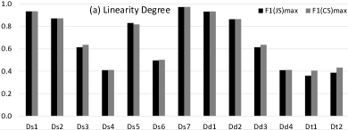
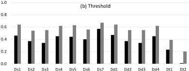
Figure 1. Degree of linearity per dataset in Table 3 (left) and the respective threshold (right) with respect to Equations 1 and 2.

5.1. Theoretical Measures

Degree of Linearity. The results for each benchmark dataset are shown in Figure 1. We observe that the linearity of six datasets exceeds 0.8 (with three exceeding 0.9) for both similarity measures, which indicates rather easy classification tasks, as the two classes can be separated by a linear classifier with high accuracy. The maximum values are obtained with $D_{s7}$, where indeed practically all DL-based algorithms achieve a perfect F-measure of F1=1.0 (Zhang et al., 2020).

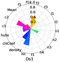
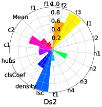
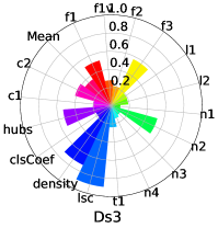
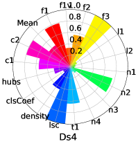
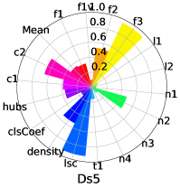
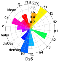
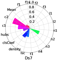
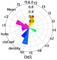
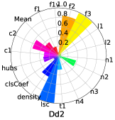
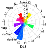
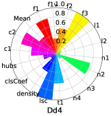
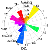
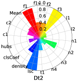
Figure 2. Complexity measures per dataset in Table 3.

There is a wide deviation between the thresholds used by the Cosine and Jaccard similarities, but the actual difference between them is rather low: $F1_{CS}^{max}$ is higher than $F1_{JS}^{max}$ by just 0.8%, on average, across the structured and dirty datasets. In the case of textual datasets, though, Cosine similarity outperforms Jaccard similarity by 12.3% on average. This is due to the large number of tokens per record, which significantly reduces the Jaccard scores.

Overall, $F1_{CS}^{max}$ and $F1_{JS}^{max}$ suggest that among the structured datasets, only $D_{s3}$, $D_{s4}$ and $D_{s6}$ are complex enough to call for non-linear classification models. The same applies only to $D_{d3}$ and $D_{d4}$ from the dirty datasets, and to both textual datasets ($D_{t1}$, $D_{t2}$).

Complexity Measures. We now present the first complexity analysis of the main benchmark datasets for matching algorithms. All measures are implemented by the problexity Python package (Komorniczak et al., 2022), using the two-dimensional feature vector defined at the end of Section 3.2. The results are shown in Figure 2.

More specifically, datasets identified as rather easy by the above linearity degree analysis achieve the lowest scores for the majority of the complexity measures, and the lowest ones on average. As expected, the lowest average score corresponds to $D_{s7}$ (0.179), since the vast majority of its individual measures falls far below 0.2. Among the remaining easy datasets ($D_{s1}$, $D_{s2}$, $D_{s5}$, $D_{d1}$ and $D_{d2}$), the maximum average score corresponds to $D_{s5}$, amounting to 0.346.

We observe that there are three datasets with an average score close to 0.346: $D_{s3}$ with 0.354, $D_{d2}$ with 0.341 and $D_{d3}$ with 0.355. Comparing them with $D_{s5}$, we observe that they get higher scores for most measures. However, $D_{s3}$ and $D_{d3}$ achieve the minimum value for $f_{2}$ among all datasets, i.e., the overlapping region between the two classes has the smallest volume among all datasets. They also exhibit comparatively low values for $f_{3}$, which implies that the two features we have defined are quite effective in separating the two classes. Most importantly, their scores for both class imbalance measures are close to the minimum score across all datasets. The reason is that they have an unrealistically high portion of positive instances, which, as shown in Table 3, is second only to that of $D_{t2}$ (which gets the lowest scores for $c_{1}$ and $c_{2}$ in Figure 2). Regarding $D_{d2}$, it exhibits scores close to the minimum ones for $l_{1}$, which indicates low distances of incorrectly classified instances from a linear classification boundary, as well as for $n_{1}$ and $n_{2}$, which indicate a low number of instances surrounded by examples from the other class. As a result, the complexity measures indicate that $D_{s3}$, $D_{d2}$ and $D_{d3}$ pose easy classification tasks, which is in line with Table 4, where most matchers achieve high $F1$ over these datasets.

All other datasets achieve an average score that fluctuates between 0.423 and 0.457. Overall, a mean complexity score below 0.400 indicates easy classification tasks, with only $D_{s4}$, $D_{s6}$, $D_{d4}$, $D_{t1}$ and $D_{t2}$ being challenging.

5.2. Practical Measures

Table 4. F1 per method and data set. Hyphen indicates insufficient memory. The highest F1 per category and dataset is in bold.

	$D_{s1}$	$D_{s2}$	$D_{s3}$	$D_{s4}$	$D_{s5}$	$D_{s6}$	$D_{s7}$	$D_{d1}$	$D_{d2}$	$D_{d3}$	$D_{d4}$	$D_{t1}$	$D_{t2}$
(a) DL-based matching algorithms
DeepMatcher (15)	98.65	95.50	88.46	69.66	75.86	65.98	95.45	96.63	93.07	75.00	46.56	68.53	94.04
DeepMatcher (40)	98.76	93.70	84.62	64.42	66.67	53.73	91.67	96.54	92.73	66.67	46.99	69.21	-
DeepMatcher (Mudgal et al., 2018)	98.40	94.00	88.00	66.90	72.70	69.30	100.00	98.10	93.80	74.50	46.00	62.80	92.70
DITTO (15)	51.46	88.62	67.61	51.44	42.62	70.66	28.76	42.29	91.21	61.73	44.15	38.94	54.60
DITTO (40)	89.43	91.18	56.82	58.02	28.00	66.94	65.67	90.16	91.05	65.06	60.80	42.09	64.77
DITTO (Li et al., 2020a)	98.99	95.60	97.06	86.76	94.37	75.58	100.00	99.03	95.75	95.65	85.69	89.33	93.85
EMTransformer-B (15)	98.99	95.42	92.59	80.80	82.35	68.14	97.78	98.88	95.24	98.04	79.59	83.94	78.31
EMTransformer-B (40)	99.21	95.38	92.31	82.72	82.35	66.20	97.78	98.99	95.53	94.34	82.81	85.42	77.65
EMTransformer-R (15)	98.87	95.90	96.15	84.83	80.00	69.04	100.00	98.19	95.78	94.12	83.95	89.29	77.65
EMTransformer-R (40)	98.52	95.83	94.55	85.04	80.00	68.36	100.00	98.30	95.22	94.34	82.69	87.11	77.12
EMTransformer (Li et al., 2020b; Brunner and Stockinger, 2020)	N/A	N/A	N/A	N/A	N/A	N/A	N/A	98.90	95.60	94.20	85.50	90.90	N/A
GNEM (10)	98.21	95.19	96.43	84.96	77.78	70.85	100.00	98.87	93.93	94.74	79.19	88.66	-
GNEM (40)	98.55	94.95	98.18	20.45	80.00	74.75	100.00	98.87	93.92	89.66	83.87	86.49	-
GNEM (Chen et al., 2020b)	N/A	N/A	N/A	86.70	N/A	74.70	N/A	N/A	N/A	N/A	N/A	87.70	N/A
HierMatcher (10)	-	94.85	-	79.37	72.00	72.06	100.00	-	-	-	58.63	-	-
HierMatcher (40)	-	94.85	-	79.37	72.00	72.06	100.00	-	-	-	58.63	-	-
HierMatcher (Fu et al., 2020)	98.80	95.30	N/A	81.60	N/A	74.90	N/A	98.01	94.50	N/A	68.50	N/A	N/A
(b) Non-neural, non-linear ML-based matching algorithms
Magellan-DT	97.65	86.88	88.52	62.37	84.85	54.42	100.00	40.07	78.76	50.00	33.89	48.46	100.00
Magellan-LR	97.66	88.61	84.21	65.99	80.00	44.44	100.00	83.20	76.03	50.00	32.77	37.36	100.00
Magellan-RF	98.32	92.96	89.66	67.76	84.85	56.10	100.00	60.47	81.67	52.00	38.06	51.30	100.00
Magellan-SVM	90.19	81.41	84.62	65.03	84.62	2.53	84.21	10.99	48.15	12.12	12.62	0.00	99.96
Magellan (Mudgal et al., 2018)	98.40	92.30	91.20	71.90	78.80	49.10	100.00	91.90	82.50	46.80	37.40	43.60	79.80
ZeroER	98.80	65.67	49.81	64.41	35.90	18.50	90.91	36.53	39.23	10.42	20.00	2.56	-
ZeroER (Wu et al., 2020)	96.00	86.00	N/A	N/A	N/A	48.00	100.00	N/A	N/A	N/A	N/A	52.00	N/A
(c) Non-neural, linear supervised matching algorithms
SA-ESDE	93.06	87.57	52.94	45.27	85.71	51.58	100.00	92.71	86.80	52.94	45.27	37.67	43.97
SAQ-ESDE	93.08	88.62	55.81	43.91	82.76	54.13	97.77	93.16	88.51	49.41	42.82	37.94	58.40
SAF-ESDE	88.84	83.14	32.43	28.51	61.54	36.36	76.92	88.94	82.64	33.71	27.29	21.24	40.08
SAS-ESDE	93.49	87.40	64.00	43.62	87.50	48.17	95.45	93.35	86.79	64.00	42.27	40.57	79.86
SB-ESDE	91.19	79.63	92.31	67.81	82.76	52.65	84.44	84.27	78.18	46.43	42.94	45.63	41.23
SBQ-ESDE	91.44	82.71	84.21	67.55	83.33	45.20	100.00	87.54	82.29	55.70	37.47	47.17	58.37
SBF-ESDE	90.89	80.69	77.27	67.34	78.57	33.88	95.65	70.36	69.91	30.43	22.27	33.91	39.12
SBS-ESDE	90.89	82.45	87.72	67.35	82.76	46.68	100.00	85.68	80.06	43.14	41.29	49.15	79.86

Setup. We conducted all experiments on a server with an Nvidia GeForce RTX 3090 GPU (24 GB RAM) and a dual AMD EPYC 7282 16-Core CPU (256 GB RAM), with all implementations running in Python. Given that every method depends on different Python versions and packages, we aggregated all of them into a Docker image, which facilitates the reproducibility of our experiments. Note that every evaluated method requires a different format for the input data; we performed all necessary transformations and will publish the resulting files and the Docker image upon acceptance.

Methods Configuration. Following (Mudgal et al., 2018), DeepMatcher is combined with fastText (Bojanowski et al., 2017) embeddings in the attribute embedding module, the Hybrid model in the attribute similarity vector module, and a two layer fully connected ReLU HighwayNet (Zilly et al., 2017) classifier followed by a softmax layer in the classification module.

EMTransformer has two different versions: EMTransformer-B and EMTransformer-R, which use BERT and RoBERTa, respectively. As noted in (Li et al., 2020b) (Section E in their Appendix), its original implementation ignores the validation set. Instead, “it reports the best F1 on the test set among all the training epochs”. To align it with the other methods, we modified its code so that it uses the validation set to select the best performing model that is applied to the testing set.

For GNEM, we employ a BERT-based embedding model, because its dynamic nature outperforms the static pre-trained models like fastText, as shown by the authors in (Bojanowski et al., 2017). In the interaction module, we apply a single-layer gated graph convolution network, following the recommendation of the authors.

DITTO employs RoBERTa, since it is best performing in (Li et al., 2020a, 2021). However, we were not able to run DITTO with part-of-speech tags, because these tags are provided by a service that was not available. Therefore, like all other methods we evaluated, DITTO did not employ any external knowledge.

HierMatcher employs the pre-trained fastText model (Bojanowski et al., 2017) for embeddings, while the hidden size of each GRU layer is set to 150 in the representation layer, following (Fu et al., 2020).

We also modified the functionality of ZeroER, decoupling it from the blocking function that is hand-crafted for each dataset. Only in this way we can ensure that it applies to exactly the same instances as all other methods, allowing for a fair comparison.

Finally, we combine Magellan with four different classification algorithms: Magellan-DT uses a Decision Tree, Magellan-LR Logistic Regression, Magellan-RF a Random Forest, and Magellan-SVM a Support Vector Machine. Similar to ZeroER, for a fair comparison, we decoupled the blocking functionality provided by Magellan, applying it to the same blocked data sets as all other methods.

Hyperparameters. Initial experiments showed that the number of epochs is probably the most important hyperparameter for most DL-based matching algorithms. To illustrate this, we report the performance of every DL algorithm for two different settings: (1) the default number of epochs as reported in the corresponding paper, and (2) 40 epochs, which is common in the original papers. Table 4 shows the resulting performance, with the number in parenthesis next to each DL-based algorithm indicating the number of epochs.

Reproducibility Analysis. To verify the validity of the above configurations, which will also be applied to the new datasets, Table 4 also presents the fine-tuned performance of each non-linear matching algorithm, as reported in the literature. The lower the difference between the best F1 performance we achieved for each method on a specific dataset and the one reported in the literature, the closer we are to the optimal configuration for this method.

Starting with the DL-based matching algorithms, our experiments with DeepMatcher exceed those of (Mudgal et al., 2018) in most cases, by 1.5%, on average. For EMTransformer, we consider the results reported in (Li et al., 2020b), because the original experiments in (Brunner and Stockinger, 2020) show the evolution of F1 across the various epochs, without presenting exact numbers. The average difference with our F1 is just 0.15% on average. Slightly higher, albeit negligible, just 0.3%, is the mean difference between our results and GNEM’s performance in (Chen et al., 2020b). Our results for HierMatcher are consistently lower than those in (Fu et al., 2020), with an average difference of 5.4%. HierMatcher constitutes a relatively reproducible algorithm. Finally, DITTO’s performance in (Li et al., 2020a) is consistently higher than our experimental results to a significant extent – on average by 25%. This is caused by the lack of external knowledge and the absence of two optimizations (see Section 3 in (Li et al., 2020a)). Yet, our best performance among all DL-based matching algorithms per dataset is very close or even higher than DITTO’s performance in (Li et al., 2020a) in all datasets, but $D_{s5}$.

Regarding the ML-based matching algorithms, Magellan underperforms the results in (Mudgal et al., 2018) in $D_{s4}$ and $D_{d1}$, while for $D_{s1}$, $D_{s2}$, $D_{s3}$, $D_{d2}$ and $D_{d4}$, the differences are minor ($\leq 1.8\%$ in absolute terms). For the remaining five datasets, though, our results are significantly higher than (Mudgal et al., 2018), by 13% on average. For ZeroER, we get slightly better performance in $D_{s1}$, while for the other four datasets examined in (Wu et al., 2020), our results are lower by 60%, on average. The reason is that (Wu et al., 2020) combines ZeroER with custom blocking methods and configurations in each case, whereas we use the same configuration in all datasets. Yet, the best performance per dataset that is achieved by one of Magellan’s variants consistently outperforms ZeroER’s performance in (Wu et al., 2020), except for $D_{t1}$, where its top F1 is 0.7% lower.

On the whole, the selected configurations provide an overall performance close to or even better than the best one for non-linear matching algorithms in the literature.

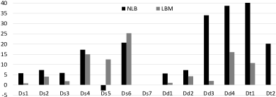
Figure 3. Practical measures per dataset in Table 3.

Aggregate Practical Measures. Figure 3 presents the non-linear boost (NLB) and the learning-based margin (LBM), as we described in Section 3.3, per dataset. Both measures should exceed 5%, ideally 10%, in a dataset that is considered as challenging. Only in such a dataset are the two classes linearly inseparable to a large extent, while there is a significant room for improvements.

Among the structured datasets, this requirement is met only by $D_{s4}$ and $D_{s6}$. The first three datasets exhibit a high NLB, demonstrating their non-linearity, but have a very low LBM, as many algorithms achieve a practically perfect performance. In $D_{s5}$, there is room for improvements, but the two classes are linearly separable to a large extent, as the best linear algorithms outperform the best non-linear ones. Finally, both measures are reduced to 0 over $D_{s7}$, because both linear and non-linear algorithms achieve perfect F1.

All dirty datasets have a higher degree of non-linearity, as indicated by their NLB, which consistently exceeds 5%. However, the first three datasets are ideally solved by the DL-based matching algorithms, especially EMTransformer, leaving $D_{d4}$ as the only challenging dataset of this type.

Finally, both textual datasets exhibit high non-linearly, but on $D_{t2}$, all Magellan variants achieve perfect performance (outperforming the DL-based matchers). Hence, only $D_{t1}$ is challenging.

6. Methodology for New Benchmarks

Table 5. Existing Vs New Benchmarks

$D_{t1}$	0.955	0.120	12.03%	$D_{n1}$	0.899	0.029	2.90%
$D_{s1}$	0.998	0.137	13.68%	$D_{n3}$	0.983	0.953	95.30%
$D_{s2}$	1.000	0.229	22.89%	$D_{n8}$	0.906	0.166	16.60%
$D_{s4}$	1.000	0.104	10.37%	$D_{n7}$	0.894	0.018	1.80%
$D_{s6}$	0.898	0.247	24.66%	$D_{n2}$	0.910	0.074	7.40%

Table 6. Characteristics of the new datasets generated by DeepBlocker (Thirumuruganathan et al., 2021). The blocking performance is reported with recall ($PC$), precision ($PQ$), the total number of candidates ($|C|$) and the number of matching candidates ($|P|$). DeepBlocker applies Autoenconder to the selected attribute(s) ($attr.$) using stemming and stop-word removal or not ($cl.$), and $K$ candidates per query record of the indexed dataset ($ind.$).

	$D_{1}$	$D_{2}$	$|D_{1}|$	$|D_{2}|$	$|A|$	Blocking performance				DeepBlocker config.				$|I_{tr}|$	$|I_{te}|$	$|P_{tr}|$	$|P_{te}|$	$|N_{tr}|$	$|N_{te}|$	IR
						$PC$	$PQ$	$|C|$	$|P|$	$attr.$	$cl.$	$K$	$ind.$
$D_{n1}$	Abt	Buy	1,076	1,076	3	0.899	0.029	33,356	967	name	$\times$	31	$D_{2}$	20,014	6,671	580	193	19,433	6,478	2.9%
$D_{n2}$	Amazon	GP	1,354	3,039	4	0.910	0.074	13,540	1,005	title	$\times$	10	$D_{1}$	8,124	2,708	603	201	7,521	2,507	7.4%
$D_{n3}$	DBLP	ACM	2,616	2,294	4	0.983	0.953	2,294	2,186	all	✓	1	$D_{2}$	1,376	459	1,312	437	65	22	95.3%
$D_{n4}$	IMDB	TMDB	5,118	6,056	5	0.898	0.011	158,658	1,768	all	✓	31	$D_{1}$	95,195	31,732	1,061	354	94,134	31,378	1.1%
$D_{n5}$	IMDB	TVDB	5,118	7,810	4	0.891	0.003	322,434	955	all	$\times$	63	$D_{1}$	193,460	64,487	573	191	192,887	64,296	0.3%
$D_{n6}$	TMDB	TVDB	6,056	7,810	6	0.927	0.130	7,810	1,015	all	✓	1	$D_{2}$	4,686	1,562	609	203	4,077	1,359	13.0%
$D_{n7}$	Walmart	Amazon	2,554	22,074	6	0.894	0.018	43,418	763	all	✓	17	$D_{1}$	26,051	8,684	458	153	25,593	8,531	1.8%
$D_{n8}$	DBLP	GS	2,516	61,353	4	0.906	0.166	12,580	2,091	all	✓	5	$D_{1}$	7,548	2,516	1,255	418	6,293	2,098	16.6%

Our methodology for creating new benchmarks consists of the following three steps:

1. Given a dataset with a complete ground truth, apply a state-of-the-art blocking method that is suitable for the data at hand. Blocking is indispensable for reducing the search space to the most likely duplicates, which can be processed by a matching algorithm within a reasonable time frame.

2. Based on the available ground truth, fine-tune the selected blocking method for a minimum level of recall. In practical situations, recall should be very high (e.g., 90%), because most learning-based matchers take decisions at the level of individual record pairs and, thus, they cannot infer duplicates not included in the candidate pairs. The fine-tuning maximizes precision for the selected recall so as to minimize the class imbalance. In this process, the selected recall level determines the difficulty of the labeled instances. The higher the recall levels are, the more difficult to classify positive instances (true matches) are included at the expense of including more and easier negative instances (true non-matches), and vice versa for low recall levels. We term “easy positive instances” the duplicate entities whose similarity is higher than most non-matching pairs, whereas “easy negative instances” involve non-matching entities with a similarity lower than most matching ones.

3. Randomly split the candidates pairs into training, validation and testing sets with a typical ratio, using the ground truth.

4. Apply all difficulty measures from Section 3 to decide whether the resulting benchmark is challenging enough.

To put this methodology into practice, we use the eight, publicly available, established datasets for RL in Table 6. They cover a wide range of domains, from product matching ($D_{n1}$, $D_{n2}$, $D_{n7}$) to bibliographic data ($D_{n3}$, $D_{n8}$) and movies ($D_{n4}$-$D_{n6}$). We apply DeepBlocker (Thirumuruganathan et al., 2021) to these datasets, a generic state-of-the-art approach leveraging Autoenconder, self-supervised learning and fastText embeddings. Through grid search, DeepBlocker is configured so that its recall, also known as pair completeness ($PC$) (Christen, 2012), exceeds 90%. Note that our methodology is generic enough to support any other blocking method and recall limit.

For every dataset, DeepBlocker generates the candidate pair set $C$ by indexing one of the two data sources ($D_{1}$ or $D_{2}$ in Table 6), while every record of the other source is used as a query that retrieves the $K$ most likely matches. To maximize precision, we consider the lowest $K$ that exceeds the minimum recall. In each dataset, we use both combinations of indexing and query sets and select the one yielding the lowest number of candidates for the required recall.

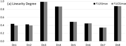
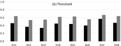
Figure 4. Degree of linearity per dataset in Table 6 (left) and the respective threshold (right) with respect to Equations 1 and 2.

We also fine-tune two more hyperparameters: (1) whether cleaning is used or not (if it does, stop-words are removed and stemming is applied to all words), and (2) the attributes providing the values to be blocked. We consider all individual attributes as well as a schema-agnostic setting that concatenates all attributes into a sentence. Note that DeepBlocker converts these attributes into embedding vectors using fastText and then applies self-supervised learning to boost its accuracy without requiring any manually labelled instances; fastText’s static nature ensures that the order of words in the concatenated text does not affect the resulting vector. For every hyperparameter, we consider all possible options and select the one minimizing the returned set of candidates. This means that we maximize precision, also known as pairs quality ($PQ$) (Christen, 2012), so as to maximize the portion of matching pairs in the resulting candidate set, minimizing the class imbalance.

The exact configuration of DeepBlocker per dataset is shown in Table 6. Column attr. indicates that the schema-agnostic setting yields the best performance in most cases, column cl. suggests that cleaning is typically required, and column ind. shows that the smallest data source is typically indexed. Finally, the number of candidates per query entity, $K$, differs widely among the datasets, depending heavily on the data at hand.

Given that DeepBlocker constitutes a stochastic approach, the performance reported in Table 6 corresponds to the average after 10 repetitions. For this reason, in some cases, $PC$ drops slightly lower than 0.9. The resulting candidate pairs are randomly split into training, validation, and testing sets with the same ratio as the benchmarks in Table 3 (3:1:1). These settings simulate the realistic scenarios, where blocking is applied to exclude obvious non-matches, and then a subset of the generated candidate pairs is labelled to train a matching algorithm that resolves the rest of the candidates. The instances per class and set are reported in Table 6 (note that the testing and validation sets have the same size).

At this point, it is worth juxtaposing the existing and the new benchmarks that have the same origin. These datasets are compared in Table 5. We observe that $D_{t1}$ and $D_{s2}$ outperform $D_{n1}$ and $D_{n8}$, respectively, both in terms of recall and precision, even though DeepBlocker outperforms Magellan’s blocking methods (Thirumuruganathan et al., 2021). Therefore, the higher precision of $D_{t1}$ and $D_{s2}$ is most likely achieved due to the removal of negative pairs. Moreover, the recall of $D_{s4}$ is lower than $D_{s7}$ by just 6%, but its precision is higher by a whole order of magnitude, whereas the recall of $D_{s6}$ is lower than $D_{n2}$ by just 1.2%, but its precision is higher by 3.3 times. These tradeoffs are not common in blocking over these two particular datasets (Papadakis et al., 2022) and could be caused by removing a large portion of negative pairs. Finally, $D_{n3}$ exhibits much higher precision (almost by 7 times) than $D_{s1}$, even though their difference in recall is just 1.5%. Given that a wide range of blocking methods achieves exceptionally high precision in this bibliographic dataset (Papadakis et al., 2022), the low precision of the existing benchmark could be caused by including a large number of easy, negative pairs, i.e. obvious non-matches. Overall, the five existing benchmarks in Table 5 seem to involve an undocumented approach for inserting or removing an arbitrary number of negative pairs.

The only exception is $D_{n3}$, which is dominated by positive candidate pairs after blocking. This indicates a rather easy RL dataset, where blocking suffices for detecting the duplicate records, rendering matching superfluous. This is due to the low levels of noise and the distinguishing information in its bibliographic data. Yet, the imbalance ratio in the respective existing benchmarks, $D_{s1}$ and $D_{d1}$, is 81% lower, which implies that they contain a large portion of obvious non-matches. This explains why $D_{s1}$ and $D_{d1}$ have been marked as easy classification tasks in the analysis of Section 5.

6.1. Analysis of new benchmarks

The above process is not guaranteed to yield challenging classification tasks for learning-based matching algorithms. For this reason, our methodology includes a third step, which assesses the difficulty of each new benchmark through the theoretical and practical measures defined in Sections 3 and 4, respectively. We should stress, though, that our methodology allows analysts to tune the difficulty level of the generated datasets by changing the level of blocking recall (90% in our case) and by replacing DeepBlocker with another state-of-the-art blocking algorithm.

6.1.1. Theoretical Measures

Degree of Linearity. In Figure 4(a), we show the values of $F1_{CS}^{max}$ and $F1_{JS}^{max}$ per dataset along with the respective thresholds. We observe that both measures exceed 0.87 for $D_{n3}$, $D_{n4}$ and $D_{n8}$, while remaining below 0.49 for all other datasets. For $D_{n3}$, this is expected, because, as explained above, it involves quite unambiguous duplicates, due to the low levels of noise. The same is also true for $D_{n8}$, which also conveys bibliographic data, with its duplicates sharing clean and distinguishing information. The opposite is true for $D_{n4}$: its low precision after blocking indicates high levels of noise and missing values, requiring many candidates per entity to achieve high recall. The fastText embeddings may add to this noise, as the attribute values are dominated by movie titles and the names of actors and directors, which are underrepresented in its training corpora. In contrast, the traditional textual similarity measures at the core of $F1_{CS}^{max}$ and $F1_{JS}^{max}$ are capable of separating linearly the two matching classes.

On the whole, these a-priori measures suggest that $D_{n1}$, $D_{n2}$, and $D_{n5}$ to $D_{n7}$ pose challenging matching tasks.

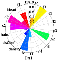
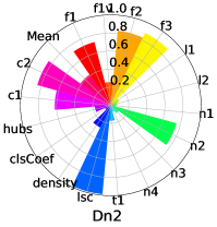
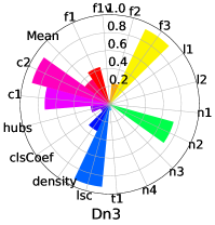
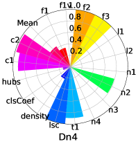
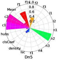
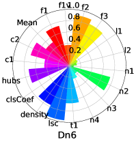
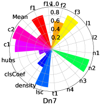
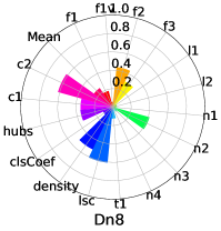
Figure 5. Complexity measures per dataset in Table 6.

Table 7. F1 per method and dataset in Tb. 6. Hyphen indicates insufficient memory. The highest F1 per category and dataset is in bold.

	$D_{n1}$	$D_{n2}$	$D_{n3}$	$D_{n4}$	$D_{n5}$	$D_{n6}$	$D_{n7}$	$D_{n8}$
(a) DL-based matching algorithms
DM(15)	70.49	52.01	99.32	90.50	59.88	69.95	56.57	95.10
DM(40)	71.43	56.15	99.32	89.73	63.18	67.28	57.14	93.51
DITTO(15)	86.43	38.10	-	86.50	66.82	-	71.73	95.31
DITTO(40)	-	67.95	-	86.84	0.59	-	63.91	95.04
EM-B(15)	84.68	64.39	99.43	91.91	67.14	77.78	67.56	93.16
EM-B(40)	85.88	65.38	99.54	91.26	-	78.54	62.86	92.98
EM-R(15)	91.35	65.49	99.43	92.51	-	79.28	67.55	94.81
EM-R(40)	-	70.12	99.54	-	-	77.56	63.29	93.21
GNEM(10)	-	-	99.43	-	-	-	62.89	95.53
GNEM(40)	-	-	99.43	-	-	-	60.05	95.34
HM(10)	-	-	-	91.39	58.52	-	63.31	-
HM(40)	-	-	-	91.39	58.52	-	63.31	-
(b) Non-neural, non-linear ML-based matching algorithms
MG-DT	52.55	41.67	99.54	91.69	59.72	56.84	50.00	91.73
MG-LR	43.84	39.19	99.66	91.25	59.64	61.10	55.65	91.06
MG-RF	57.42	44.44	99.66	92.64	61.11	59.74	61.18	93.82
MG-SVM	-	-	98.20	91.01	59.34	61.01	61.67	88.70
ZeroER	32.66	22.14	99.32	43.32	0.50	53.76	61.52	84.14
(c) Non-neural, linear supervised matching algorithms
SA-ESDE	47.79	40.35	98.64	85.75	47.86	43.98	34.41	88.24
SAQ-ESDE	44.59	41.41	98.64	82.80	49.93	43.96	37.77	88.57
SAF-ESDE	20.27	28.09	98.75	82.69	49.25	44.20	29.08	76.38
SAS-ESDE	47.97	39.58	98.75	77.41	49.53	44.22	35.19	87.47
SB-ESDE	49.62	46.87	99.66	61.95	58.87	60.50	66.13	89.95
SBQ-ESDE	52.95	49.79	99.66	20.00	7.61	54.26	34.07	91.36
SBF-ESDE	36.64	36.52	99.66	20.00	7.61	53.81	33.40	85.41
SBS-ESDE	53.65	45.39	99.66	20.00	7.61	53.60	33.43	88.29

Complexity Measures. TThese are presented in Figure 5. The average complexity score is lower than 0.40 for $D_{n3}$ and $D_{n8}$ (0.339 and 0.251, respectively), in line with the degree of linearity, but it exceeds this threshold for $D_{n4}$ (0.431). This is caused by its very low imbalance ratio (see also Table 6), which results in high scores for the class imbalance measures and some of the feature overlapping ones. In all other cases, though, it exhibits the (second) lowest score among all datasets, including the established ones. Note also that $D_{n5}$ yields a very low average score (0.282), that surpasses only $D_{n8}$. This indicates a rather easy classification task, because of the very low values ($\ll$0.2) for 9 out of the 17 complexity measures. Hence, only $D_{n1}$, $D_{n2}$, $D_{n6}$ and $D_{n7}$ correspond to challenging, non-linearly separable matching benchmarks.

6.1.2. Practical Measures

For the DL-based matching algorithms, we use the same configurations as for the existing benchmarks in Table 4, due to their high performance, which matches or surpasses the literature. The results appear in Table 7, while Figure 5 reports the non-linear boost (NLB) and the learning-based margin (LBM).

For the datasets marked as challenging by the theoretical measures ($D_{n1}$, $D_{n2}$, $D_{n6}$ and $D_{n7}$), both practical measures take values well above 5%. LBM takes its minimum value (8.7%) over $D_{n1}$, as EMTransformer with RoBERTa performs exceptionally well, outperforming all other DL-based algorithms by at least 5% and all others by at least 34%. NLB takes its minimum value over $D_{n7}$, because the F1 for SB-ESDE is double as that of all other linear algorithms, reducing is distance from the top DL-based one to 5.6%.

Among the remaining datasets, all algorithms achieve perfect performance over $D_{n3}$, thus reducing both practical measures to 0. The same applies to a lesser extent to $D_{n8}$, where both measures amount to $\sim$4.3%. In $D_{n4}$ and $D_{n5}$, both practical measures exceed 5% to a significant extent. The reason for the former is that the best DL- and ML-matchers lie in the middle between the perfect F1 and the best linear algorithm, whose performance matches the degree of linearity. For $D_{n5}$, the practical measures are in line with the degree of linearity, unlike the complexity measures, which suggest low levels of difficulty.

Overall, the practical measures suggest that, with the exception of $D_{n3}$ and $D_{n8}$ (which exhibit linear separability of their classes), all other datasets are challenging enough for assessing the relative performance of DL-based matchers.

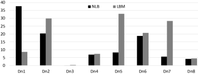
Figure 6. Practical measures per dataset in Table 6.

6.2. Memory Consumption and Run-times.

We now investigate the space and time requirements of all matching algorithms across the nine selected datasets. The results are shown in Figure 7.

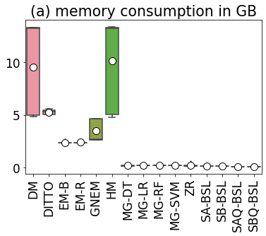
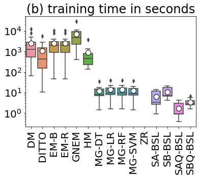
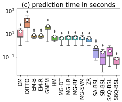
Figure 7. Memory and time requirements per algorithm across the datasets $D_{s4}$, $D_{s6}$, $D_{d3}$, $D_{d4}$, $D_{t1}$, $D_{n1}$, $D_{n2}$, $D_{n6}$, $D_{n7}$.

Starting with Figure 7(a), we observe that all baseline methods occupy $\leq$200 MB, on average, because their space complexity is dominated by the input data. In contrast, the space requirements of the DL-based algorithms is determined by their embeddings and their learned model, which together increase the memory consumption by an entire order of magnitude. The most frugal among them is EMTransformer, which occupies $\sim$2.5 GB on every dataset, regardless of the underlying language model. The reason is that it involves a simple local, heterogeneous operation, which leverages language models in a straightforward manner. Hence, its space complexity is dominated by its 768-dimensional embeddings vectors.

The next most memory efficient approach is DeepMatcher, which requires 10 GB, on average ($\sim$14 GB on every existing and $\sim$5.3 GB on every new dataset). This is determined by the 300-dimensional fastText vectors and the hybrid attribute summarization.

The remaining DL-based algorithms run out of memory in at least one case, making it hard to assess their actual memory consumption. DITTO fails in just three cases, while requiring $\sim$5.5 GB in all other cases. This is determined by the 768-dimensional RoBERTa vectors and the additional records generated during the data augmentation process. GNEM fails in three new datasets for both number of epochs, while requiring $\sim$3.7 GB, on average, in all other cases. The higher memory consumption of GNEM should be attributed to its global operation, which uses a graph to model the relations between all candidate pairs. Finally, HierMatcher has the highest memory consumption among all DL-based algorithms, as it is able to process only four of the nine benchmark datasets. In these cases, it requires 10.6 GB, on average. Its high space complexity should be attributed to its complex, hierarchical neural network, which computes contextual fastText vectors for each token and performs cross-attribute token alignment in one of its layers.

Regarding the training times, their distribution is shown in Figure 7(b). As indicated by the log-scale of the vertical axis, the baseline methods are more efficient by at least two orders of magnitude. Magellan requires just 13 seconds, on average, with minor variations among the various classifiers. Our threshold-based baselines are even faster, fluctuating between 1 (SAQ-BSL) and 10 (SB-BSL) seconds per dataset, on average.

For the DL-based algorithms, the training time is determined to a large extent by the number of epochs. The most efficient training corresponds to HierMatcher: 8 and 22 min for 10 and 40 epochs, respectively, on average. However, these measurements probably overestimate its time efficiency, as they capture only the four datasets where HierMatcher is applicable. The second shortest training time is achieved by DITTO, with an average of 12 and 24 min for 15 and 40 epochs, resp. Both times would probably be higher if DITTO was fully applicable to all datasets. The third place involves all methods that apply to all datasets, namely DeepMatcher and EMTransformer with both language models. Despite their fundamentally different functionality, their training takes 23 (61) min for 15 (40) epochs, on average. The most time consuming training corresponds to GNEM: 65 (167) min for 10 (40) epochs, but is most likely even higher over the datasets, where it ran out of memory. Again, this is caused by its global operation.

The most important aspect of time efficiency is the prediction time in Figure 7(c). The difference between the non-neural and the DL-based approaches is again high, but does not exceed the two orders of magnitude. The fastest approaches are our threshold-based baselines, which process every dataset in (far) less than 1 second. They are followed by ZeroER and Magellan, which both require $\sim$4 seconds per dataset, on average. The fastest DL-based approach is HierMatcher, with a mean of $\sim$6 seconds. This is overestimated, though, due to the missing cases. The next fastest approach is EMTransformer, which takes $\sim$8 seconds per dataset, in the average case. This high efficiency stems from the simple, local operation that applies the selected language model in a straightforward manner. DeepMatcher requires twice as much time (i.e., $\sim$16s), on average, due to the higher complexity of its hybrid attribute summarization model. GNEM is much slower, with $\sim$40 seconds per dataset, on average, due to its global operation that examines the relations between all candidate pairs. Yet, the most time-consuming prediction corresponds to DITTO, which depends on the number of epochs (unlike all other DL-based matchers): it requires $\sim$109 and $\sim$219 seconds for 15 and 40 epochs, respectively. This should be attributed to the attribute normalization and the TF-IDF-based summarization of long attribute values, due to its heterogeneous functionality.

7. Conclusions

We make the following observations: (1) The datasets used for benchmarking matching algorithms should be evaluated both a-priori, through their degree of linearity and complexity, and a-posteriori, through the aggregate measures summarizing the performance of linear and non-linear matchers. Excelling in all these respects is necessary for datasets that leave enough room for improvements by complex, DL-based classifiers. (2) Most of the popular datasets used as benchmarks for DL-based matchers involve almost linearly separable candidate pairs, or are perfectly solved by most existing matching algorithms (therefore, leaving no room for improvement). These characteristics render these datasets unsuitable for benchmarking matching algorithms. (3) We experimentally demonstrate that the proposed methodology for creating new ER benchmarks leads to datasets that are better suited for assessing the benefits of DL-based matchers. Moreover, our methodology is flexible, and can be used to produce benchmark datasets with a tunable degree of difficulty. In order to promote further progress, we make all our code and datasets available through a Docker image.

In the future, we plan to examine whether different configurations for DeepBlocker, or different blocking methods can extract challenging benchmarks from one of the easy datasets, like the bibliographic ones (DBLP-ACM and DBLP-Google Scholar). We actually intend to create a series of datasets that cover the entire continuum of benchmark difficulty.

Appendix

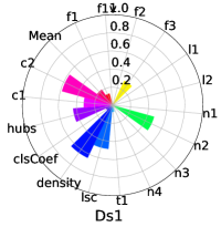
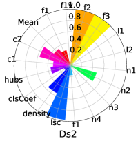
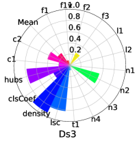
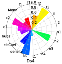
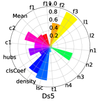
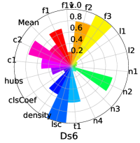
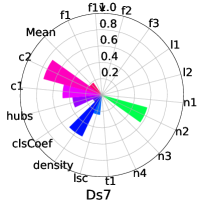
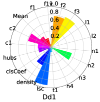
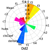
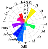
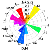
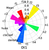
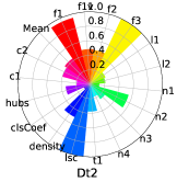
Figure 8. Schema-based complexity measures per dataset in Table 3.

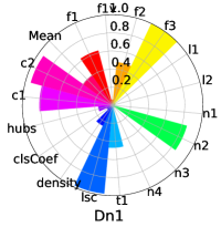
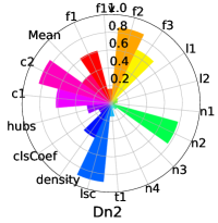
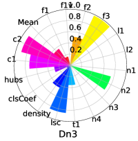
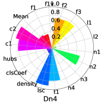
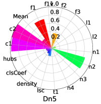
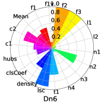
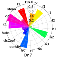
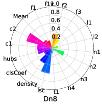
Figure 9. Schema-based complexity measures per dataset in Table 6.

A. Schema-based Theoretical Measures

The a-priori measures in Section 3 leverage schema-agnostic settings, which disregard the attribute values associated with every record. It is possible, though, to adapt them to a schema-aware functionality. Algorithm 1 can actually be restricted to the tokens of a specific attribute in a straightforward way.

Moreover, the complexity measures in Section 3.2 can be coupled with the Cosine and Jaccard similarities that are calculated for each attribute, representing every candidate pair $c_{i,j}$ through the multi-dimensional feature vector:

$$f_{i,j}=[CS^{a_{1}}(c_{i,j}),JS^{a_{1}}(c_{i,j}),\ldots,CS^{|A|}(c_{i,j}),JS^{|A|}(c_{i,j}),]$$

where $x^{a_{k}}(c_{i,j})$ denotes the $x\in\{CS,JS\}$ similarity over the values of attribute $a_{k}\in A$, while $A$ stands for the set of all attributes describing the records in the input dataset $D$, with $|A|$ being the number of attributes in $D$. The actual value of the complexity measures when using this multi-dimensional feature vector appear in Figures 8 and 9 for the existing and the new benchmarks in Tables 3 and 6, respectively.

Comparing Figure 8 with Figure 2, we observe significant variation among the individual measures. Inevitably, the same applies to the mean score across all measures. Yet, using a mean value of 0.4 as the threshold for distinguishing between easy and difficult benchmarks, we are led to the same conclusion: only datasets $D_{s4}$ (0.409), $D_{s6}$ (0.467), $D_{d4}$ (0.438), $D_{t1}$ (0.423) and $D_{t2}$ (0.431) are challenging, as all others have an average score well below this threshold, fluctuating between 0.183 ($D_{s7}$) and 0.386 ($D_{d3}$).

The same pattern appears in Figure 9; there is a significant fluctuation between the individual measures, but when comparing the average one to the cut-off threshold (0.4), the challenging datasets are the , same as the schema-agnostic settings in Figure 5: $D_{n1}$, $D_{n2}$, $D_{n6}$ and $D_{n7}$.

B. Existing Benchmark Datasets

This section compares in more detail the characteristics of the existing benchmark datasets with those created by following our proposed approach in Section 6.

Starting with the generation process, the datasets typically used for benchmarking learning-based matching algorithms (i.e., the datasets in Table 3) stem from the Magellan repository (note that some publications on the topic use additional datasets, but only the ones in Table appear in multiple publications). Their generation process was originally described at: https://sites.google.com/site/anhaidgroup/useful-stuff/the-magellan-data-repository/description-of-the-784-data-sets and repeated in https://github.com/anhaidgroup/deepmatcher/blob/master/Datasets.md. It involves the following steps for most datasets:

1. Given the two tables (tableA.csv and tableB.csv), perform dataset specific blocking to obtain a candidate set $C$.

2. For each tuple pair in set $C$, if the pair is present in the golden matches file (gold.csv), mark the pair as a match. Else, mark the pair as a non-match.

3. Randomly split the labeled candidate set C into 3 sets, i.e., train, validation, and test, with ratio 3:1:1.

The procedure is slightly different for $D_{s5}$:

1. Crawled HTML pages from the two websites.

2. Extracted tuples from the HTML pages to create two tables, one per site.

3. Performed blocking on these tables (to remove obviously non-matched tuple pairs), producing a set of candidate tuple pairs.

4. Took a random sample of pairs from the above set and labeled the pairs in the sample as “match” / “non-match”.

In both cases, there is no reference to the blocking method that was used and to its parameter configuration (e.g., which attributes were considered in the creation of blocks?). The blocking configuration typically has a significant impact on the resulting performance (Zeakis et al., 2023; Papadakis et al., 2022). This means that the dataset generation process is not reproducible and that there is no way of evaluating its outcomes. In general, a loose blocking approach achieves high recall, ensuring that all positive pairs are included in the labeled instances, at the cost of including many negative pairs with low similarity, which can thus be easily discarded by a learning-based matching algorithm, even a linear one. In contrast, a strict blocking approach might sacrifice a small part of the positive pairs, but mostly includes highly similar negative pairs, which are harder to be classified, thus requiring more effective, complex and non-linear learning-based matching algorithms. DeepBlocker, with its high effectiveness, ensures that only negative pairs involving nearest neighbors are included in the labeled instances, without sacrificing a significant portion of the positive

As a result of this unclear generation pnrocess, the imbalance ratio of the datasets generated by our methodology in Section 6, which leverages DeepBlocker, is much lower than that in the existing benchmark datasets, even though the difference in recall is low. More specifically, we focus on the datasets in Tables 3 and 6 that have the same origin, which are $D_{s1}$-$D_{n3}$, $D_{s2}$-$D_{n8}$, $D_{s4}$-$D_{n7}$, $D_{s6}$-$D_{n2}$ and $D_{t1}$-$D_{n1}$. Note that for $D_{s1}$, $D_{s2}$, $D_{s6}$ and $D_{t1}$, we rely on the original version of the datasets released by (Köpcke et al., 2010). For $D_{s6}$, we use the statistics of the website that provides this dataset. For the corresponding new benchmarks datasets, we use the clean versions employed in a series of past publications (e.g., (Gagliardelli et al., 2022; Zeakis et al., 2023; Papadakis et al., 2022)).

Table 8 compares the number of entities and duplicates per dataset.

Table 8. Characteristics of the datasets lying at the core of ER benchmarks

	Original Dataset			Clean Version			Existing	New
	$D_{1}$ Entities	$D_{2}$ Entities	Duplicates	$D_{1}$ Entities	$D_{2}$ Entities	Duplicates	Dataset	Dataset
Abt-Buy	1,081	1,092	1,097	1,076	1,076	1,076	$D_{t1}$	$D_{n1}$
DBLP-ACM	2,616	2,294	2,224	2,616	2,294	2,224	$D_{s1}$	$D_{n3}$
DBLP-GS	2,616	64,263	5,347	2,516	61,353	2,308	$D_{s2}$	$D_{n8}$
Walmart-Amazon	2,554	22,074	962	2,554	22,074	853	$D_{s4}$	$D_{n7}$
Amazon-GP	1,363	3,226	1,300	1,354	3,039	1,104	$D_{s6}$	$D_{n2}$

We observe that the two versions agree only in DBLP-ACM. For Abt-Buy, DBLP-GS and Amazon-GP, the clean version involves both fewer entities and fewer duplicates than the original one, because the latter matches multiple entities from D1 with the same entity in D2 and vice versa. This is evident in Abt-Buy and DBLP-GS by the fact that the number of duplicates is higher than the number of D1 and/or D2 entities. These settings are in conflict with the definition of Record Linkage (aka Clean-Clean ER) (Christophides et al., 2015), which requires that every data source is individually duplicate-free. For this reason, the clean versions of these datasets have removed all entities involved in the contradictory matches. In the case of the Walmart-Amazon dataset, we kept all entities, but removed the contradictory matches from the ground truth.

Based on these generic characteristics, Table 5 compares the ER-specific measures per dataset.

We observe that in Abt-Buy and DBLP-GS, the existing benchmark outperforms the new one both with respect to recall and precision, even though the latter uses a much more effective blocking method than the former (Thirumuruganathan et al., 2021) (note also that the configuration of DeepBlocker has been optimized through grid search in order to maximize the precision of the new benchmarks). Therefore, the higher precision of the existing benchmarks is most likely achieved due to the removal of negative pairs.

For the Walmart-Amazon and Amazon-GP pairs of datasets, the existing benchmarks offer a different balance between recall and precision. In the former pair, the recall of the existing benchmark is lower than the new one by just 6%, while its precision is higher by a whole order of magnitude. In the latter pair, the recall of the existing benchmark is lower than the new one by just 1.2%, while its precision is higher by 3.3 times. These tradeoffs are not common in blocking over these two particular datasets and could be caused by removing a large portion of negative pairs.

The opposite is true in the case of DBLP-ACM, where the new benchmark exhibits much higher precision (almost by 7 times) than the existing one, even though their difference in recall is just 1.5%. Given that a wide range of blocking methods achieves exceptionally high precision in this bibliographic dataset, the low precision of the existing benchmark could be caused by including a large number of easy, negative pairs.

Overall, all five dataset pairs seem to involve an undocumented approach for inserting or removing an arbitrary number of negative pairs.

References

- (1)
- DMd (2018) 2018. DeepMatcher data repository. https://github.com/anhaidgroup/deepmatcher/blob/master/Datasets.md.
- Acheampong et al. (2021) Francisca Adoma Acheampong, Henry Nunoo-Mensah, and Wenyu Chen. 2021. Transformer models for text-based emotion detection: a review of BERT-based approaches. Artif. Intell. Rev. 54, 8 (2021), 5789–5829.
- Barella et al. (2018) Victor H. Barella, Luís Paulo F. Garcia, Marcilio C. P. de Souto, Ana Carolina Lorena, and André C. P. L. F. de Carvalho. 2018. Data Complexity Measures for Imbalanced Classification Tasks. In IEEE International Joint Conference on Neural Networks IJCNN. 1–8.
- Barlaug and Gulla (2021) Nils Barlaug and Jon Atle Gulla. 2021. Neural Networks for Entity Matching: A Survey. Transactions on Knowledge Discovery from Data 15, 3 (2021).
- Binette and Steorts (2022) Olivier Binette and Rebecca C Steorts. 2022. (Almost) all of entity resolution. Science Advances 8, 12 (2022), eabi8021.
- Bojanowski et al. (2017) Piotr Bojanowski, Edouard Grave, Armand Joulin, and Tomás Mikolov. 2017. Enriching Word Vectors with Subword Information. Trans. Assoc. Comput. Linguistics 5 (2017), 135–146.
- Brunner and Stockinger (2020) Ursin Brunner and Kurt Stockinger. 2020. Entity Matching with Transformer Architectures - A Step Forward in Data Integration. In EDBT. 463–473.
- Cappuzzo et al. (2020) Riccardo Cappuzzo, Paolo Papotti, and Saravanan Thirumuruganathan. 2020. Creating Embeddings of Heterogeneous Relational Datasets for Data Integration Tasks. In SIGMOD. 1335–1349.
- Chen et al. (2020a) Deli Chen, Yankai Lin, Wei Li, Peng Li, Jie Zhou, and Xu Sun. 2020a. Measuring and Relieving the Over-Smoothing Problem for Graph Neural Networks from the Topological View. In AAAI. 3438–3445.
- Chen et al. (2020b) Runjin Chen, Yanyan Shen, and Dongxiang Zhang. 2020b. GNEM: A Generic One-to-Set Neural Entity Matching Framework. In WWW. 1686–1694.
- Christen (2012) Peter Christen. 2012. Data Matching – Concepts and Techniques for Record Linkage, Entity Resolution, and Duplicate Detection. Springer.
- Christen et al. (2023) Peter Christen, David J. Hand, and Nishadi Kirielle. 2023. A Review of the F-Measure: Its History, Properties, Criticism, and Alternatives. ACM Comput. Surv. (2023). https://doi.org/10.1145/3606367
- Christen et al. (2020) Peter Christen, Thilina Ranbaduge, and Rainer Schnell. 2020. Linking Sensitive Data – Methods and Techniques for Practical Privacy-Preserving Information Sharing. Springer, Heidelberg.
- Christophides et al. (2021) Vassilis Christophides, Vasilis Efthymiou, Themis Palpanas, George Papadakis, and Kostas Stefanidis. 2021. An Overview of End-to-End Entity Resolution for Big Data. ACM Comput. Surv. 53, 6 (2021), 127:1–127:42.
- Christophides et al. (2015) Vassilis Christophides, Vasilis Efthymiou, and Kostas Stefanidis. 2015. Entity Resolution in the Web of Data. Morgan & Claypool Publishers.
- Devlin et al. (2019) Jacob Devlin, Ming-Wei Chang, Kenton Lee, and Kristina Toutanova. 2019. BERT: Pre-training of Deep Bidirectional Transformers for Language Understanding. In NAACL-HLT. 4171–4186.
- Devlin et al. (2018) Jacob Devlin, Ming-Wei Chang, Kenton Lee, and Kristina Toutanova. 2018. Bert: Pre-training of deep bidirectional transformers for language understanding. arXiv preprint arXiv:1810.04805 (2018).
- Dong and Srivastava (2015) Xin Luna Dong and Divesh Srivastava. 2015. Big Data Integration. Morgan and Claypool Publishers.
- Ebraheem et al. (2018) Muhammad Ebraheem, Saravanan Thirumuruganathan, Shafiq R. Joty, Mourad Ouzzani, and Nan Tang. 2018. Distributed Representations of Tuples for Entity Resolution. Proc. VLDB Endow. 11, 11 (2018), 1454–1467.
- Foxcroft et al. (2019) Jeremy Foxcroft, Adrian d’Alessandro, and Luiza Antonie. 2019. Name2vec: Personal names embeddings. In Canadian Conference on Artificial Intelligence. Springer, 505–510.
- Fu et al. (2020) Cheng Fu, Xianpei Han, Jiaming He, and Le Sun. 2020. Hierarchical Matching Network for Heterogeneous Entity Resolution. In IJCAI. 3665–3671.
- Gagliardelli et al. (2022) Luca Gagliardelli, George Papadakis, Giovanni Simonini, Sonia Bergamaschi, and Themis Palpanas. 2022. Generalized Supervised Meta-blocking. Proc. VLDB Endow. 15, 9 (2022), 1902–1910.
- Goodfellow et al. (2016) Ian Goodfellow, Yoshua Bengio, and Aaron Courville. 2016. Deep Learning. MIT Press. http://www.deeplearningbook.org.
- Gower (1971) John C Gower. 1971. A general coefficient of similarity and some of its properties. Biometrics (1971), 857–871.
- Hand and Christen (2018) David J. Hand and Peter Christen. 2018. A note on using the F-measure for evaluating record linkage algorithms. Statistics and Computing 28, 3 (2018), 539–547.
- Herzog et al. (2007) T.N. Herzog, F. Scheuren, and W.E. Winkler. 2007. Data Quality and Record Linkage Techniques. Springer Verlag.
- Jain et al. (2021) Arjit Jain, Sunita Sarawagi, and Prithviraj Sen. 2021. Deep indexed active learning for matching heterogeneous entity representations. Proceedings of the VLDB Endowment 15, 1 (2021), 31–45.
- Kasai et al. (2019) Jungo Kasai, Kun Qian, Sairam Gurajada, Yunyao Li, and Lucian Popa. 2019. Low-resource Deep Entity Resolution with Transfer and Active Learning. In Annual Meeting of the Association for Computational Linguistics. Florence, 5851–5861.
- Komorniczak et al. (2022) Joanna Komorniczak, , and Pawel Ksieniewicz. 2022. problexity — an open-source Python library for binary classification problem complexity assessment. arXiv preprint arXiv:2207.06709 (2022).
- Konda et al. (2016) Pradap Konda, Sanjib Das, Paul Suganthan G. C., AnHai Doan, Adel Ardalan, Jeffrey R. Ballard, Han Li, Fatemah Panahi, Haojun Zhang, Jeffrey F. Naughton, Shishir Prasad, Ganesh Krishnan, Rohit Deep, and Vijay Raghavendra. 2016. Magellan: Toward Building Entity Matching Management Systems. Proc. VLDB Endow. 9, 12 (2016), 1197–1208.
- Köpcke et al. (2010) Hanna Köpcke, Andreas Thor, and Erhard Rahm. 2010. Evaluation of entity resolution approaches on real-world match problems. Proc. VLDB Endow. 3, 1 (2010), 484–493.
- Lan et al. (2019) Zhenzhong Lan, Mingda Chen, Sebastian Goodman, Kevin Gimpel, Piyush Sharma, and Radu Soricut. 2019. Albert: A lite bert for self-supervised learning of language representations. arXiv preprint arXiv:1909.11942 (2019).
- Leone et al. (2022) Manuel Leone, Stefano Huber, Akhil Arora, Alberto García-Durán, and Robert West. 2022. A Critical Re-evaluation of Neural Methods for Entity Alignment. Proc. VLDB Endow. 15, 8 (2022), 1712–1725.
- Li et al. (2020c) Bing Li, Wei Wang, Yifang Sun, Linhan Zhang, Muhammad Asif Ali, and Yi Wang. 2020c. GraphER: Token-Centric Entity Resolution with Graph Convolutional Neural Networks. In AAAI Conference on Artificial Intelligence, Vol. 34. 8172–8179.
- Li et al. (2020a) Yuliang Li, Jinfeng Li, Yoshihiko Suhara, AnHai Doan, and Wang-Chiew Tan. 2020a. Deep Entity Matching with Pre-Trained Language Models. Proc. VLDB Endow. 14, 1 (2020), 50–60.
- Li et al. (2020b) Yuliang Li, Jinfeng Li, Yoshihiko Suhara, AnHai Doan, and Wang-Chiew Tan. 2020b. Deep Entity Matching with Pre-Trained Language Models. CoRR abs/2004.00584 (2020).
- Li et al. (2021) Yuliang Li, Jinfeng Li, Yoshihiko Suhara, Jin Wang, Wataru Hirota, and Wang-Chiew Tan. 2021. Deep Entity Matching: Challenges and Opportunities. ACM J. Data Inf. Qual. 13, 1 (2021), 1:1–1:17.
- Liu et al. (2019a) Yinhan Liu, Myle Ott, Naman Goyal, Jingfei Du, Mandar Joshi, Danqi Chen, Omer Levy, Mike Lewis, Luke Zettlemoyer, and Veselin Stoyanov. 2019a. Roberta: A robustly optimized bert pretraining approach. arXiv preprint arXiv:1907.11692 (2019).
- Liu et al. (2019b) Yinhan Liu, Myle Ott, Naman Goyal, Jingfei Du, Mandar Joshi, Danqi Chen, Omer Levy, Mike Lewis, Luke Zettlemoyer, and Veselin Stoyanov. 2019b. RoBERTa: A Robustly Optimized BERT Pretraining Approach. CoRR abs/1907.11692 (2019).
- Lorena et al. (2018) A Lorena, L Garcia, Jens Lehmann, M Souto, and T Ho. 2018. How complex is your classification problem. A survey on measuring classification complexity. arXiv (2018).
- Mikolov et al. (2013a) Tomas Mikolov, Kai Chen, Greg Corrado, and Jeffrey Dean. 2013a. Efficient estimation of word representations in vector space. arXiv preprint arXiv:1301.3781 (2013).
- Mikolov et al. (2013b) Tomas Mikolov, Ilya Sutskever, Kai Chen, Greg S Corrado, and Jeff Dean. 2013b. Distributed representations of words and phrases and their compositionality. Advances in neural information processing systems 26 (2013).
- Mudgal et al. (2018) Sidharth Mudgal, Han Li, Theodoros Rekatsinas, AnHai Doan, Youngchoon Park, Ganesh Krishnan, Rohit Deep, Esteban Arcaute, and Vijay Raghavendra. 2018. Deep Learning for Entity Matching: A Design Space Exploration. In SIGMOD. 19–34.
- Naumann and Herschel (2010) F. Naumann and M. Herschel. 2010. An Introduction to Duplicate Detection. Morgan and Claypool Publishers.
- Newcombe et al. (1959) H.B. Newcombe, J.M. Kennedy, SJ Axford, and AP James. 1959. Automatic linkage of vital records. Science 130, 3381 (1959), 954–959.
- Ni et al. (2021) Jianmo Ni, Chen Qu, Jing Lu, Zhuyun Dai, Gustavo Hernández Ábrego, Ji Ma, Vincent Y Zhao, Yi Luan, Keith B Hall, Ming-Wei Chang, et al. 2021. Large dual encoders are generalizable retrievers. arXiv preprint arXiv:2112.07899 (2021).
- Nie et al. (2019) Hao Nie, Xianpei Han, Ben He, Le Sun, Bo Chen, Wei Zhang, Suhui Wu, and Hao Kong. 2019. Deep Sequence-to-Sequence Entity Matching for Heterogeneous Entity Resolution. In International Conference on Information and Knowledge Management. ACM, Beijing, China, 629–638.
- Paganelli et al. (2022) Matteo Paganelli, Francesco Del Buono, Andrea Baraldi, and Francesco Guerra. 2022. Analyzing How BERT Performs Entity Matching. Proc. VLDB Endow. 15, 8 (2022), 1726–1738.
- Paganelli et al. (2021) Matteo Paganelli, Francesco Del Buono, Pevarello Marco, Francesco Guerra, and Maurizio Vincini. 2021. Automated machine learning for entity matching tasks. In EDBT.
- Papadakis et al. (2022) George Papadakis, Marco Fisichella, Franziska Schoger, George Mandilaras, Nikolaus Augsten, and Wolfgang Nejdl. 2022. How to reduce the search space of Entity Resolution: with Blocking or Nearest Neighbor search? CoRR abs/2202.12521 (2022). https://arxiv.org/abs/2202.12521
- Papadakis et al. (2021) George Papadakis, Ekaterini Ioannou, Emanouil Thanos, and Themis Palpanas. 2021. The Four Generations of Entity Resolution. Morgan and Claypool.
- Papadakis et al. (2020) George Papadakis, Dimitrios Skoutas, Emmanouil Thanos, and Themis Palpanas. 2020. Blocking and Filtering Techniques for Entity Resolution: A Survey. Comput. Surveys 53, 2 (2020), 1–42.
- Peeters and Bizer (2021) Ralph Peeters and Christian Bizer. 2021. Dual-Objective Fine-Tuning of BERT for Entity Matching. Proc. VLDB Endow. 14, 10 (2021), 1913–1921.
- Pennington et al. (2014) Jeffrey Pennington, Richard Socher, and Christopher D Manning. 2014. Glove: Global vectors for word representation. In Proceedings of the 2014 conference on empirical methods in natural language processing (EMNLP). 1532–1543.
- Sagi et al. (2016) Tomer Sagi, Avigdor Gal, Omer Barkol, Ruth Bergman, and Alexander Avram. 2016. Multi-Source Uncertain Entity Resolution at Yad Vashem: Transforming Holocaust Victim Reports into People. In SIGMOD. 807–819.
- Sanh et al. (2019) Victor Sanh, Lysandre Debut, Julien Chaumond, and Thomas Wolf. 2019. DistilBERT, a distilled version of BERT: smaller, faster, cheaper and lighter. CoRR abs/1910.01108 (2019).
- Thirumuruganathan et al. (2021) Saravanan Thirumuruganathan, Han Li, Nan Tang, Mourad Ouzzani, Yash Govind, Derek Paulsen, Glenn M. Fung, and AnHai Doan. 2021. Deep Learning for Blocking in Entity Matching: A Design Space Exploration. Proc. VLDB Endow. 14, 11 (2021), 2459–2472.
- Tu et al. (2022) Jianhong Tu, Ju Fan, Nan Tang, Peng Wang, Chengliang Chai, Guoliang Li, Ruixue Fan, and Xiaoyong Du. 2022. Domain Adaptation for Deep Entity Resolution. In ACM Conference on Management of Data. Philadelphia.
- Villani and Villani (2009) Cédric Villani and Cédric Villani. 2009. The wasserstein distances. Optimal Transport: Old and New (2009), 93–111.
- Wang et al. (2022) Tianshu Wang, Hongyu Lin, Cheng Fu, Xianpei Han, Le Sun, Feiyu Xiong, Hui Chen, Minlong Lu, and Xiuwen Zhu. 2022. Bridging the Gap between Reality and Ideality of Entity Matching: A Revisiting and Benchmark Re-Construction. arXiv preprint arXiv:2205.05889 (2022).
- Wang et al. (2020) Zhengyang Wang, Bunyamin Sisman, Hao Wei, Xin Luna Dong, and Shuiwang Ji. 2020. CorDEL: A Contrastive Deep Learning Approach for Entity Linkage. In ICDM. 1322–1327.
- Wu et al. (2020) Renzhi Wu, Sanya Chaba, Saurabh Sawlani, Xu Chu, and Saravanan Thirumuruganathan. 2020. Zeroer: Entity resolution using zero labeled examples. In Proceedings of the 2020 ACM SIGMOD International Conference on Management of Data. 1149–1164.
- Yang et al. (2019) Zhilin Yang, Zihang Dai, Yiming Yang, Jaime G. Carbonell, Ruslan Salakhutdinov, and Quoc V. Le. 2019. XLNet: Generalized Autoregressive Pretraining for Language Understanding. In NeurIPS. 5754–5764.
- Yao et al. (2021) Zijun Yao, Chengjiang Li, Tiansi Dong, Xin Lv, Jifan Yu, Lei Hou, Juanzi Li, Yichi Zhang, and Zelin Dai. 2021. Interpretable and Low-Resource Entity Matching via Decoupling Feature Learning from Decision Making. In ACL/IJCNLP. 2770–2781.
- Zeakis et al. (2023) Alexandros Zeakis, George Papadakis, Dimitrios Skoutas, and Manolis Koubarakis. 2023. Pre-trained Embeddings for Entity Resolution: An Experimental Analysis. Proc. VLDB Endow. 16, 9 (2023), 2225–2238.
- Zeng et al. (2021) Kaisheng Zeng, Chengjiang Li, Lei Hou, Juanzi Li, and Ling Feng. 2021. A comprehensive survey of entity alignment for knowledge graphs. AI Open 2 (2021), 1–13.
- Zhang et al. (2020) Dongxiang Zhang, Yuyang Nie, Sai Wu, Yanyan Shen, and Kian-Lee Tan. 2020. Multi-Context Attention for Entity Matching. In WWW. 2634–2640.
- Zhang et al. (2022) Rui Zhang, Bayu Distiawan Trisedya, Miao Li, Yong Jiang, and Jianzhong Qi. 2022. A benchmark and comprehensive survey on knowledge graph entity alignment via representation learning. The VLDB Journal (2022), 1–26.
- Zhao and He (2019) Chen Zhao and Yeye He. 2019. Auto-EM: End-to-end Fuzzy Entity-Matching using Pre-trained Deep Models and Transfer Learning. In The World Wide Web Conference. ACM, San Francisco, USA, 2413–2424.
- Zhao and Fernandez (2022) Zixuan Zhao and Raul Castro Fernandez. 2022. Leva: Boosting Machine Learning Performance with Relational Embedding Data Augmentation. In SIGMOD. 1504–1517.
- Zilly et al. (2017) Julian Georg Zilly, Rupesh Kumar Srivastava, Jan Koutník, and Jürgen Schmidhuber. 2017. Recurrent Highway Networks. In ICML, Vol. 70. 4189–4198.