ESGCN: Edge Squeeze Attention Graph Convolutional Network
for Traffic Flow Forecasting

Abstract

Traffic forecasting is a highly challenging task owing to the dynamical spatio-temporal dependencies of traffic flows. To handle this, we focus on modeling the spatio-temporal dynamics and propose a network termed Edge Squeeze Graph Convolutional Network (ESGCN) to forecast traffic flow in multiple regions. ESGCN consists of two modules: W-module and ES module. W-module is a fully node-wise convolutional network. It encodes the time-series of each traffic region separately and decomposes the time-series at various scales to capture fine and coarse features. The ES module models the spatio-temporal dynamics using Graph Convolutional Network (GCN) and generates an Adaptive Adjacency Matrix (AAM) with temporal features. To improve the accuracy of AAM, we introduce three key concepts. 1) Using edge features to directly capture the spatio-temporal flow representation among regions. 2) Applying an edge attention mechanism to GCN to extract the AAM from the edge features. Here, the attention mechanism can effectively determine important spatio-temporal adjacency relations. 3) Proposing a novel node contrastive loss to suppress obstructed connections and emphasize related connections. Experimental results show that ESGCN achieves state-of-the-art performance by a large margin on four real-world datasets (PEMS03, 04, 07, and 08) with a low computational cost.

1 Introduction

Traffic flow forecasting is a core component of intelligent transportation systems. It is essential for analyzing traffic situations and aims at predicting the future traffic flow of regions using historical traffic data. However, this task is challenging because of the heterogeneity and dynamic spatio-temporal dependence of traffic data.

Traffic data can be modeled using Graph Neural Networks (GNNs). In such networks, the regions are represented as nodes and flows between regions as edges. Graph Convolutional Network (GCN) is a type of GNN commonly used to handle traffic flow forecasting tasks. It can adequately leverage the graph structure and aggregate node information Wu et al. (2019, 2020); Kong et al. (2020); Song et al. (2020); Li and Zhu (2021). Because the edges define the intensity of the adjacency matrix in a graph operation, accurate edge graph is an important factor in determining the performance of a GCN. Recent studies focus on capturing the connection patterns via an adaptive adjacency matrix (AAM) that is found in the training process BAI et al. (2020a); Wu et al. (2019). In our study, we focus on enhancing the AAM with the following three distinctive features.

First, we propose an Edge Squeeze (ES) module that directly uses spatio-temporal flows with edge features to construct an AAM. Recent studies in GCN revealed that edge features are equally important as node features Gong and Cheng (2019); Chen and Chen (2021). While the edge features can be used to simulate the traffic flows between regions, to the best of our knowledge this is the first study to build an adjacency matrix from the edge features in this task. Existing methods use node embeddings which cannot accurately reflect the relationship among nodes because the embedding vectors are fixed for inference and only represent spatial nodes. Therefore, they cannot handle dynamic patterns occurred in the inference and are unable to accurately capture spatio-temporal features. However, the ES module leverages the temporal features directly to construct the AAM and reflects the changes of temporal features in the inference. ES module creates three-dimensional (3D) spatio-temporal correlations beyond the spatial-specific embeddings.

Second, we develop a novel edge attention mechanism. We further explore the edge features with the attention mechanism to refine the AAM. Because the edge features represent the adjacency relations, we apply the attention mechanism to activate meaningful edges and suppress the others of the adjacency matrix. The edge attention exploits feature’s channel information such as SENet Hu et al. (2020), referred to as the squeeze attention. Existing methods apply transformer attention mechanism Vaswani et al. (2017) which presents high computational burden. The channel attention mechanism provides relatively lower computation cost and can generate more refined AAM.

Third, we introduce a novel node contrastive loss. Previous studies computed the similarities between the node embeddings that were trained with a forecasting objective function for the AAM. This method generated the adjacency matrix without an explicit objective for the shape of the graph, consequently inducing suboptimal performance. To overcome this, we maximize the difference between related and unrelated nodes to facilitate separation of the forecasting relevant nodes from the residuals. This aids in preventing the propagation of information on unrelated nodes through AAM.

Additionally, we propose a backbone network, W-module, to extract multi-scale temporal features for traffic flow forecasting. W-module is a fully convolutional network that consists of node-wise convolution to handle time-series features of each node separately. Owing to its non-autoregressive attributes and receptive field of convolution layers, the W-module can extract multiple levels of temporal features from shallow to deep layers and provide a hierarchical decomposition. We combine the ES module with W-module and propose ESGCN to forecast traffic flow. The main contributions of this study are summarized as follows:

• We propose an end-to-end framework (ESGCN) using two novel modules: ES module and W-module. ESGCN effectively learns hidden and dynamic spatio-temporal relationships using edge features.

• We introduce an edge attention mechanism and node contrastive loss to construct an AAM which captures accurately the relationships among nodes.

• We perform extensive experiments on four real-world datasets (PEMS03, 04, 07, and 08); the results shows that ESGCN achieves state-of-the-art performance by a large margin with a low computational cost.

2 Related Work

GCN for traffic forecasting. GCN is a special type of convolutional neural network that is widely used in traffic forecasting tasks Hechtlinger et al. (2017); Kipf and Welling (2017). Recurrent-based GCN adopts a recurrent architecture, such as LSTM and replaces inner layers with GCN Li et al. (2018); Bai et al. (2020b). This type of GCN handles spatial and temporal features recurrently, however it has long-range memory loss problem. STGCN Yu et al. (2017), GSTNet Fang et al. (2019), and Graph WaveNet Wu et al. (2019) use fully convolutional architecture and graph operation. They exploit spatial and temporal convolution separately to model spatio-temporal data. These methods show relatively fast inference speed and improved performance on long-range temporal data.

Attention mechanism for traffic forecasting. Attention mechanisms are used to effectively capture spatio-temporal dynamics for traffic forecasting. ASTGCN  Guo et al. (2019), GMAN Zheng et al. (2020), and STGRAT Park et al. (2020) exploited the attention mechanism which considers changes in road speed and diverse influence of spatial and temporal network. Existing approaches leveraged transformer attention Vaswani et al. (2017) that computes key, query and value relations. Contrastingly, our proposed network adopts a channel attention such as SENet Hu et al. (2020) and CBAM Woo et al. (2018) which have relatively low computation cost and high speed.

Adaptive Adjacency Matrix Construction. Previous studies used a predefined adjacency matrix for GCN Li et al. (2018); Yu et al. (2017); Yao et al. (2019); Guo et al. (2019). In a previous study, a spatial AAM was proposed as a supplementary for the predefined adjacency matrix for graph WaveNet Wu et al. (2019). STGAT Kong et al. (2020) also utilized the AAM, however, they were limited by spatial dependencies. AGCRN Bai et al. (2020b) exploited an AAM solely based on spatial node embedding. In this study, we introduce a spatio-temporal based AAM that captures accurate relations.

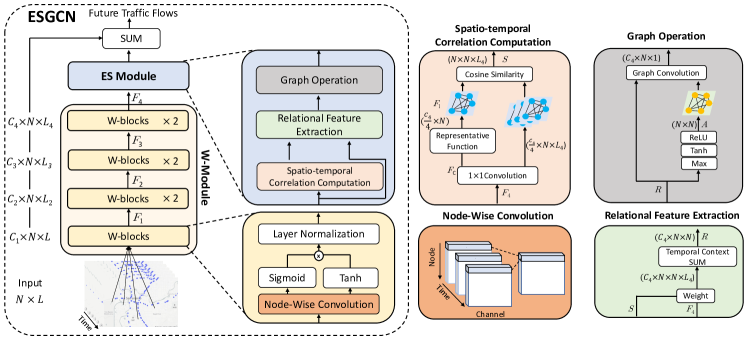
Figure 1: Overall architecture of ESGCN. ESGCN comprises the ES module and W-module consisting of four stages. Each stage of the W-module consists of multiple W-blocks, namely gated node-wise convolution layers with a layer normalization. The ES module computes the spatio-temporal correlation, generates an adaptive adjacency matrix with attention mechanism, and finally conducts GCN.

3 Problem Definition

To predict future traffic, univariate time-series data from each region ${\{X_{1},X_{2},X_{3},\dots\}}$ are provided where $X_{i}\in\mathbb{R}^{n}$ is the traffic record at time step $i$ and $n$ is the number of regions. The purpose is to find a function $\mathcal{E}$ that is capable of predicting the future of length $o$ by analyzing existing $T$-length past data. Traffic flows are generated for multiple regions and the problem is formulated as follows:

$$\{X_{t+1},\dots,X_{t+o}\}=\mathcal{E}(X_{t-T+1},\dots,X_{t}),$$ (1)

where $t$ is an arbitrary time step.

4 Proposed Method

This section describes the edge squeeze graph convolution network (ESGCN). The network comprises two modules: W-module and edge squeeze (ES) module, as shown in Fig. 1. W-module extracts region-specific temporal features and ES module produces an AAM using temporal features with an edge attention and 3D spatio-temporal relations.

4.1 W-Module

W-module extracts the time-series features of each node and is split into four W-block groups as illustrated in Fig. 1. We call each group as stage. To organize the W-module, we use a combination of gated node-wise convolutions (GNC) and a layer normalization Ba et al. (2016), namely W-block as the smallest unit. GNC has two node-wise convolution layers: one for embedding features with a tanh function and the other for gating with a sigmoid function, as shown in Fig. 1. The two outputs are multiplied element-wise and summarized as follows:

$$GNC(X)=sigmoid(\mathcal{C}(X))\circ tanh(\mathcal{C}(X)),$$ (2)

where $\mathcal{C}$ is a 2D convolution layer with a 1 $\times$ 3 kernel and 0$\times$1 padding, and $\circ$ is element-wise multiplication. $X$ is an input feature of $X\in\mathbb{R}^{c\times n\times t}$, where $c$ is the number of channels, $n$ is the number of nodes, and $t$ is an arbitrary temporal dimension. This 1$\times$3 convolution layer is referred to as node-wise convolution. Given that the convolution kernel has a size of one in the node dimension and expands the receptive field in the time dimension, the W-block is only responsible for extracting temporal features. The output features of the GNC are fed to the layer normalization layer. Each stage has 1, 2, 2, and 2 W-blocks with a stride of 1 for first stage and a stride of 2 for the others. The output of $i^{th}$ stage is defined as $F_{i}\in\mathbb{R}^{~{}c_{i}\times n\times\frac{l}{2^{i-1}}}$, where $c_{i}$ is specified as a hyperparameter and $l$ is input time-series length.

The receptive field of convolution layer expands as the feature passes through the various stages. Therefore, the features of the early stages capture local signals and subtle changes and the features of late stages are learned for global signals and overall movements. To take this advantages in handling multiple levels of signal size, the outputs of the intermediate stages are also used with the last output features for the final prediction. In W-module, each stage has 3, 9, 12, and 12 receptive field sizes in a sequential order. This can decompose the time-series hierarchically and each stage is efficiently trained to be responsible for possible signals.

4.2 Edge Squeeze Module

The ES module is a spatio-temporal feature extractor, which enhances temporal features with relations from the W-module. As described in Fig. 1, it reflects the node relations through three steps: spatio-temporal correlation computation, relational feature extraction, and GCN operation.

Spatio-temporal correlation computation. In this step, we construct spatio-temporal correlations to model flows among nodes. The modeling involves three steps. First, we feed the last features of W-module, $F_{4}$, to a single convolution layer to reduce the channel size and computation cost. This is defined as:

$$F_{c}=\mathcal{C}(F_{4}),F_{c}\in\mathbb{R}^{~{}\frac{c_{4}}{4}\times n\times l_{4}},$$ (3)

where $\mathcal{C}$ is $1\times 1$ convolution of output channels and $l_{4}$ is $\frac{l}{8}$.

Second, we extract a temporal representative from $l_{4}$ temporal nodes in each region to compute spatio-temporal correlations between the representatives ($n$) and all nodes ($n\times l_{4}$). The node is set in the last time step as a representative node. This is inspired by the Markov decision process (MDP) Bellman and Howard (1961), which considers only a state of current time step to decide an action at the subsequent time, and the representative of node is the closest value to the prediction value of the last element on the time dimension. The representative function $\mathcal{T}$ is as follows:

$$F_{l}=\mathcal{T}(F_{c}),~{}F_{l}\in\mathbb{R}^{~{}c_{4}\times n},$$ (4)

where $F_{l}$ denotes the last node on the time dimension.

Finally, the relations between the features and the representatives are computed. The original feature, $F_{c}$ has $n\times l_{4}$ nodes, and representative, $F_{l}$ has $n$ nodes. The spatio-temporal correlations between $F_{c}$ and $F_{l}$ are in $n\times n\times l_{4}$ space. Inspired by previous studies Wu et al. (2019); Li and Zhu (2021); Kong et al. (2020), a similarity function is adopted to measure the correlations between spatio-temporal nodes. The cosine similarity is adopted for this study. The result of cosine similarity is bounded from -1 to 1, and it is suitable for comparing high-dimensional features  Luo et al. (2018). The cosine similarity $cos$ is defined as follows:

$$cos(x_{1},x_{2})=\frac{x_{1}\cdot x_{2}}{\|x_{1}\|_{2}\cdot\|x_{2}\|_{2}},$$ (5)

where $\cdot$ is dot product and $\|\cdot\|_{2}$ is Euclidean norm. The final spatio-temporal correlations $S$ is defined as:

$$S=cos(F_{l},F_{c}),~{}S\in\mathbb{R}^{n\times n\times l_{4}}$$ (6)

Relational features extraction. Based on the previous step, each node has $n\times l_{4}$ correlations. We employ these correlations to weight $F_{4}$ and generate correlation-aware features, $\in\mathbb{R}^{c_{4}\times n\times l_{4}}$, for each node. Subsequently, we aggregate the temporal channel features, $l_{4}$, to reflect temporal contexts. To facilitate computation, we expand the dimension of $S$ to $S^{e}\in\mathbb{R}^{n\times c_{4}\times n\times l_{4}}$ (1 to $c_{4}$) and define $S_{i}^{e}\in\mathbb{R}^{c_{4}\times n\times l_{4}}$ as the correlation of the $i^{th}$ node. In following equations, $z(:,:,*)$ denotes $*^{th}$ tensor of $z$ on the last dimension. The computation process is defined as:

$$R(:,:,k)=\sum_{j\in l_{4}}S_{k}^{e}(:,:,j)\circ F_{4}(:,:,j),$$ (7)

where $R(:,:,k)\in\mathbb{R}^{c_{4}\times n}$ is the $k^{th}$ node’s relational features between all nodes, $k=1,2,\dots,n$.

We use the relational features as a feature matrix for graph convolution. This has an advantage over other features as it reflects temporal relations. GCN conducts operation only considering of spatial node relations. However, in spatio-temporal data, temporal relations need to be included. In the relational features, each node has $n$ different nodes created by considering temporal contexts. Thus, we use $R(:,:,k)$ tensor as $n$ neighbor nodes with $c_{4}$ dimension to predict $k^{th}$ node future flow. It can reflect the temporal relations in the relational features and spatial relations in GCN operation.

GCN operation. GCN requires a feature matrix and an adjacency matrix. As previously mentioned, the relational features are used as the feature matrix. To construct the adjacency matrix, we apply an attention mechanism to the relational features. Inspired by SENet Hu et al. (2020) and CBAM Woo et al. (2018), we adopt a channel attention mechanism known as squeeze attention to refine the AAM from the relational features. The squeeze attention activates important spatial and channel positions. Therefore, we use this mechanism to extract the edge positions’ importance. To squeeze the edge features, we feed the relational features to max operation, tanh, and ReLU activation as following:

$$A=ReLU(tanh(max(R)))$$ (8)

The outcome, $A\in n\times n$, is the generated AAM. The graph operation with $A$ and $R$ is defined as:

$$F_{g}(:,k)=W\otimes R(:,:,k)\otimes A(k,:)+B,$$ (9)

where $F_{g}(:,k)\in\mathbb{R}^{c_{4}}$ represents features for $k^{th}$ node, $W$ is a learnable weight denoted as $W\in\mathbb{R}^{c_{4}\times c_{4}}$, $B$ is a bias as $B\in R^{c_{4}}$, and $\otimes$ is matrix multiplication.

4.3 ESGCN

The proposed framework consists of the W-module and ES module. The outputs of the first three stages of the W-module and ES module are employed to access all levels of features. The computation process is summarized as follows:

$$P=\sum_{i=1}^{t-1}\mathcal{C}^{~{}i}(F_{i})+\mathcal{C}^{e}(F_{g}),$$ (10)

where $t$ is the number of stages, $\mathcal{C}^{~{}i}$ and $\mathcal{C}^{e}$ are a $1\times 1$ convolution layer for the $i$-th stage and ES module respectively.

To predict future flow, two fully connected layers with ReLU activation function are used. $P$ is fed to the two fully connected layers.

$$\hat{Y}=W_{b}\otimes ReLU(W_{a}\otimes P+B_{a})+B_{b},~{}\hat{Y}\in\mathbb{R}^{~{}h\times n},$$ (11)

where $W_{a}$ and $W_{b}$ are weights and $B_{a}$ and $B_{b}$ are bias of the fully connected layers and $h$ is the number of time steps in the prediction.

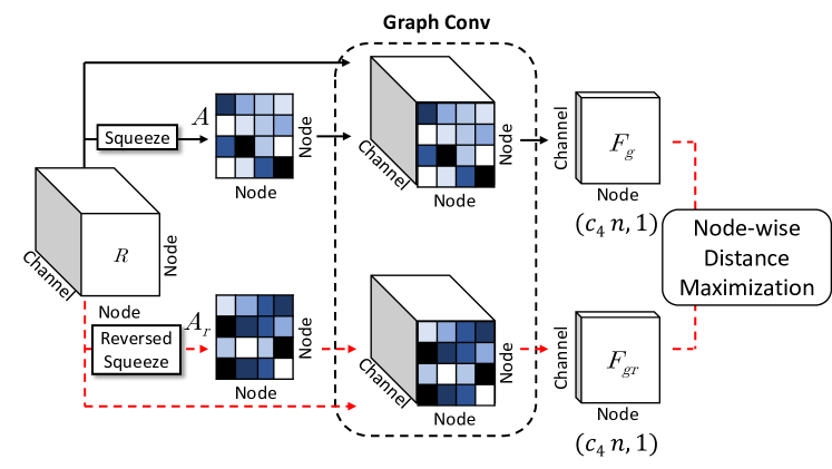
Figure 2: Proposed the node contrastive loss implementation. Note the branch with red dashed line is solely used for loss computation and not for inference.

4.4 Loss Function

We adopt the Huber loss and the proposed node contrastive loss. Huber loss is defined as follows:

$$h\big{(}\hat{Y},Y\big{)}=\left\{\begin{aligned} &\frac{1}{2}(\hat{Y}-Y)^{2},&|\hat{Y}-Y|<\delta\\ &\delta|\hat{Y}-Y|-\frac{1}{2}\delta^{2},&|\hat{Y}-Y|\geq\delta\end{aligned}\right.,$$ (12)

where $\delta$ is set to 1, $\hat{Y}$ denotes predicted values and $Y$ is ground truth values. The objective function, $L_{h}$ is defined as follows:

$$L_{h}=\frac{1}{b\times o}\sum\limits_{k=1}^{b}\sum\limits_{i=1}^{o}h(\hat{Y}_{i}^{k},Y_{i}^{k}),$$ (13)

where $\hat{Y}_{i}^{k}$ and $Y_{i}^{k}$ are the predicted value and ground truth of $i$-th time step of $k$-th sample in a mini batch respectively, and $b$ is the number of samples in a mini batch.

Node contrastive loss. This is used to effectively separate related and unrelated nodes. As shown in Fig. 2, the reversed adjacency matrix, $A_{r}$, is generated. We modify the squeeze function as follows:

$$A_{r}=ReLU(-tanh(max(R)))$$ (14)

Subsequently, the unrelated features are extracted using the graph operation in the reversed adjacency matrix. Finally, we maximize the distance between the related features, $F_{g}$, with the original adjacency matrix and the unrelated features, $F_{gr}$, with the reversed adjacency matrix. The node contrastive loss is defined as:

$$L_{n}=\frac{1}{n}tr(F_{g}^{T}\otimes F_{gr}),$$ (15)

where $tr$ is the trace of a matrix and $F_{g}^{T}\in\mathbb{R}^{~{}n\times c_{4}}$ denotes a transposed matrix. Minimizing an orthogonal of the multiplied matrix can be viewed as reducing the similarity between corresponding nodes based on a dot product.

The final loss function is calculated as follows:

$$L=L_{h}+\lambda L_{n},$$ (16)

where $\lambda$ is set to 0.1 in our experiments.

Dataset	Metric	STGCN$\dagger$	ASTGCN$\dagger$	Graph WaveNet$\dagger$	GMAN*	STSGCN$\dagger$	AGCRN*	STFGNN$\dagger$	ESGCN
PEMS03	RMSE	30.12 $\pm$ 0.70	29.66 $\pm$ 1.68	32.94 $\pm$ 0.18	27.92 $\pm$ 1.15	29.21 $\pm$ 0.56	28.19 $\pm$ 0.20	28.34$\pm$ 0.46	25.01 $\pm$ 0.34
	MAE	17.49 $\pm$ 0.46	17.69 $\pm$ 1.43	19.85 $\pm$ 0.03	16.87 $\pm$ 0.31	17.48 $\pm$ 0.15	15.93 $\pm$ 0.08	16.77 $\pm$ 0.09	15.05 $\pm$ 0.07
	MAPE	17.15 $\pm$ 0.45	19.40 $\pm$ 2.24	19.31 $\pm$ 0.49	18.23 $\pm$ 0.01	16.78 $\pm$ 0.20	14.97 $\pm$ 0.17	16.30 $\pm$ 0.09	14.32 $\pm$ 0.01
PEMS04	RMSE	35.55 $\pm$ 0.75	35.22 $\pm$ 1.90	39.70 $\pm$ 0.04	30.71 $\pm$ 0.09	33.65 $\pm$ 0.20	32.35 $\pm$ 0.22	31.88$\pm$ 0.14	30.38 $\pm$ 0.10
	MAE	22.70 $\pm$ 0.64	22.93 $\pm$ 1.29	25.45 $\pm$ 0.03	19.16 $\pm$ 0.04	21.19 $\pm$ 0.10	19.76 $\pm$ 0.09	19.83 $\pm$ 0.06	18.88 $\pm$ 0.05
	MAPE	14.59 $\pm$ 0.21	16.56 $\pm$ 1.36	17.29 $\pm$ 0.24	13.40 $\pm$ 0.01	13.90 $\pm$ 0.05	13.13 $\pm$ 0.35	13.02 $\pm$ 0.05	12.70 $\pm$ 0.01
PEMS07	RMSE	38.78 $\pm$ 0.58	42.57 $\pm$ 3.31	42.78 $\pm$ 0.07	-	39.03 $\pm$ 0.27	35.09 $\pm$ 0.10	35.80 $\pm$ 0.18	33.93 $\pm$ 0.28
	MAE	25.38 $\pm$ 0.49	28.05 $\pm$ 2.34	26.85 $\pm$ 0.05	-	24.26 $\pm$ 0.14	21.17 $\pm$ 0.13	22.07 $\pm$ 0.11	20.55 $\pm$ 0.10
	MAPE	11.08 $\pm$ 0.18	13.92 $\pm$ 1.65	12.12 $\pm$ 0.41	-	10.21 $\pm$ 1.65	8.97 $\pm$ 0.07	9.21 $\pm$ 0.07	8.61 $\pm$ 0.01
PEMS08	RMSE	27.83 $\pm$ 0.20	28.16 $\pm$ 0.48	31.05 $\pm$ 0.07	24.71 $\pm$ 0.13	26.80 $\pm$ 0.18	25.69 $\pm$ 0.21	26.22 $\pm$ 0.15	24.59 $\pm$ 0.15
	MAE	18.02 $\pm$ 0.14	18.61 $\pm$ 0.40	19.13 $\pm$ 0.08	15.69 $\pm$ 0.02	17.13 $\pm$ 0.09	16.22 $\pm$ 0.13	16.64 $\pm$ 0.09	15.56 $\pm$ 0.10
	MAPE	11.40 $\pm$ 0.10	13.08 $\pm$ 1.00	12.68 $\pm$ 0.57	10.04 $\pm$ 0.01	10.96 $\pm$ 0.07	10.50 $\pm$ 0.20	10.60 $\pm$ 0.06	9.88 $\pm$ 0.08
Comp. cost	# Param.	384,243	450,031	311,400	229,569	2,872,686	748,810	3,873,580	199,062
	Train	9.14	31.79	29.30	86.9	43.16	21.57	43.02	26.65
	Test	6.92	3.69	2.19	9.0	48.45	2.43	48.45	3.02

Table 1: Performance and computation cost comparison of ESGCN and baseline models on PEMS03, PEMS04, PEMS07 and PEMS08 datasets. The values in bold indicates the best performances. The experiments are repeated ten times. MAPE metric is measured as a percentage. Comp. cost denotes computational cost. The Train is average time in seconds per epoch and the Test is total time of running test dataset in seconds. The computation costs are computed on the same machine with the same mini batch size on PEMS04 dataset. $\dagger$: Experimental results are excerpted from [Li and Zhu, 2021] *: Experiment is conducted by us. For all metrics, a smaller value denotes superior performance.

5 Experiments

5.1 Implementation Details

The proposed model is trained with an Adam optimizer  Kingma and Ba (2015) for 50 epochs. The initial learning rate is 0.0003 and reduced by 0.7 every 5 epochs. The weight decay factor for L2 regulation is set to 0.0001, and the batch size is set to 30 for PEMS07 and 64 for PEMS03, 04, and 08. Training sessions are conducted on an NVIDIA Tesla V100 and Intel Xeon Gold 5120 CPU.

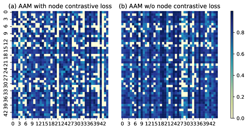
Figure 3: Heatmap of AAM with and without node contrastive loss on the first 45 nodes.

5.2 Datasets

Datasets	Nodes	MissingRatio	Range
PEMS03	358	0.672%	9/1/2018 - 11/30/2018
PEMS04	307	3.182%	1/1/2018 - 2/28/2018
PEMS07	883	0.452%	5/1/2017 - 8/31/2017
PEMS08	170	0.696%	7/1/2016 - 8/31/2016

Table 2: Dataset description and statistics.

The framework is validated on four real-world traffic datasets, namely: PEMS03, PEMS04, PEMS07, and PEMS08  Song et al. (2020). Table 2 shows the description of each dataset. These four datasets contain generated traffic flows in four different regions of California using the Caltrans Performance Measurement System. Time-series data are collected at 5-minute intervals. Standard normalization and linear interpolation are used for stable training. For a fair comparison, all datasets are split into training, validation, and test data at a ratio of 6 : 2 : 2. Twelve time steps (1 h) are used to predict the next 12 time steps (1 h) and all experiments are repeated 10 times with random seeds. The test data performance is verified by selecting the model of the epoch that showed the best performance in the validation data.

5.3 Baseline Methods

ESGCN is compared with the following models on the same hyperparameters and official implementations:

• STGCN: Spatio-temporal graph convolutional networks, which comprise spatial and temporal dilated convolutions Yu et al. (2017).

• ASTGCN: Attention-based spatial temporal graph convolutional networks, which adopt spatial and temporal attention into the model Guo et al. (2019).

• GraphWaveNet: Graph WaveNet exploits an adaptive adjacency graph and dilated 1D convolution Wu et al. (2019).

• GMAN: Graph multi-attention network uses spatial and temporal attention in graph neural network Zheng et al. (2020).

• STSGCN: Spatial–temporal synchronous graph convolutional networks, which utilize a spatio-temporal graph that extends the spatial graph to the temporal dimension Song et al. (2020).

• AGCRN: Adaptive graph convolutional recurrent network for traffic forecasting. This model exploits node adaptive parameter learning and an adaptive graph Bai et al. (2020b).

• STFGNN: Spatial–temporal fusion graph neural networks, which leverage fast-DTW to construct a spatiotemporal graph Li and Zhu (2021).

Case	ES module	Node contrastive loss	Attention Op.	$\lambda$	Rep. function	RMSE	MAE	MAPE(%)
1			-	-	-	30.69	19.12	12.91
2	✓		Max	-	Last	30.45	18.94	12.80
3(ours)	✓	✓	Max	0.1	Last	30.38	18.88	12.72
4	✓	✓	Max	0.3	Last	30.41	18.89	12.78
5	✓	✓	Max	0.5	Last	30.62	18.98	12.74
6	✓	✓	Max	0.7	Last	30.40	18.92	12.79
7	✓	✓	Max	0.9	Last	30.64	18.99	12.80
8	✓	✓	Avg	0.1	Last	30.46	18.98	12.91
9	✓	✓	Max + L	0.1	Last	30.48	18.89	12.87
10	✓	✓	Max	0.1	Middle	30.55	19.04	12.80
11	✓	✓	Max	0.1	First	30.64	19.12	12.87

Table 3: Ablation experiments on the PEMS04 dataset. Attention Op. , $\lambda$, and Rep. function denote Attention Operation, $\lambda$ weight for node contrastive loss, and representative function. Max, Avg, Max + L denote Max operation, Average operation, and Max operation with learnable layers. Last, Middle, and Last are representative node positions.

5.4 Comparison with the Baseline Methods

The proposed model is compared with state-of-the-art models. ESGCN outperformed all other baselines in terms of RMSE, MAE, and MAPE, as shown in Table 1. Compared to the current best performing models in each dataset (PEMS07: AGCRN, PEMS03,04, and 08: GMAN), ESGCN yields 4%, 2.7%, and 3.8% relative improvements on average for all datasets in RMSE, MAE, and MAPE. Graph WaveNet and AGCRN employ the AAM and STFGNN uses a non-adaptive spatio-temporal adjacency matrix. Compared to these methods, the proposed model showed superior performance and guaranteed the effectiveness of our AAM which is refined with attention and node contrastive loss. Based on the experimental results, ESGCN, has improved representation ability and exhibits promising forecasting performance.

5.5 Computational Cost

To evaluate the computational cost, we compare the number of parameters, the training time, and the inference time of our model with those of baselines in Table 1. ESGCN has the smallest parameters compared to other baselines. In training time, ESGCN is faster than STFGNN and slightly slower than AGCRN. ESGCN has the third-fastest inference speed. Although AGCRN shows faster training and inference time, specifically, 5 and 0.6 s in training and inference, respectively, the differences are insignificant. Additionally, AGCRN requires three times more parameters than ours. Especially, our model which has the channel attention shows faster running speed and includes fewer parameters than GMAN which leverages the transformer attention. Considering its superior performance, ESGCN has an acceptable computational cost.

5.6 Ablation Study

5.6.1 Components

To validate the proposed ES module and the node contrastive loss, we conduct experiments (cases 1-3) as shown in Table 3. The model with only W-module (case 1) shows the lowest performance. However, the W-module with the ES module which reflects traffic flows using GCN (case 2) achieves significant improvement. ESGCN, consisting of the W-module, ES module, and the node contrastive loss (case 3) outperforms the others. This highlights that the feature enhancement ability of ES module and the proposed loss function.

5.6.2 Attention operation

To extract important adjacency relations, our edge attention used max operation to squeeze channel features. However, CBAM Woo et al. (2018) also uses average operation to squeeze channel features. In this section, we conduct an ablation study (cases 3, 8, and 9) on the attention operation in Table 3. We empirically discovered that the max operation is the most optimal setting. Notably, the attention function with learnable layer (case 9) shows a lower performance because dimension reduction of the layer disturbs to extract the AAM Wang et al. (2020).

5.6.3 Node contrastive loss

We use a hyperparameter $\lambda$ to balance the Huber loss and node contrastive loss. Although the node contrastive loss assists in the construction of the refined AAM, an excessive effect of this loss can negatively affect forecasting performance. We empirically determine the magnitude of $\lambda$. The experimental results (cases 3-7) are shown in Table 3. Based on the results, the optimal value of $\lambda$ is 0.1. We set $\lambda$ as 0.1 across in all the experiments. In Fig 3, it shows additionally sparse AAM in which unrelated connections are removed.

5.6.4 Representative function

The representative function of ES module extracts temporal representatives on time dimension. Inspired by MDP, the representative function returns the last step node of $F_{c}$. To test whether the last node can be a temporal representative, we conduct an experiment by replacing the last node with the first node, $F_{c}(:,:,0)$, and the middle node, $F_{c}(:,:,l_{4}/2)$. The experiment results (cases 3,10, and 11) are shown in Table 3. The closer the node to the initial time step is, the lower the performance. Our representative function is based on the assumption the closest value to the prediction value can be the representatives. This ablation study empirically shows the assumption is reasonable.

6 Conclusion and Future Work

This study proposes a novel method, ESGCN, to address traffic flow forecasting. Experiments show that the proposed model achieves state-of-the-art performance on four real-world datasets and has the smallest parameters with relatively faster inference and training speed. In the future, given that ESGCN is designed as a general framework to handle spatio-temporal data, it can be applied to other applications that have spatio-temporal data structures such as regional housing market prediction and electricity demand forecasting.

References

- Ba et al. [2016] Jimmy Ba, J. Kiros, and Geoffrey E. Hinton. Layer normalization. ArXiv, abs/1607.06450, 2016.
- BAI et al. [2020a] LEI BAI, Lina Yao, Can Li, Xianzhi Wang, and Can Wang. Adaptive graph convolutional recurrent network for traffic forecasting. In Advances in Neural Information Processing Systems, volume 33, pages 17804–17815, 2020.
- Bai et al. [2020b] Lei Bai, Lina Yao, Can Li, Xianzhi Wang, and Can Wang. Adaptive graph convolutional recurrent network for traffic forecasting. arXiv preprint arXiv:2007.02842, 2020.
- Bellman and Howard [1961] R. Bellman and R. Howard. Dynamic programming and markov processes. Mathematics of Computation, 15:217, 1961.
- Chen and Chen [2021] Jun Chen and Hao-Peng Chen. Edge-featured graph attention network. ArXiv, abs/2101.07671, 2021.
- Fang et al. [2019] Shen Fang, Qi Zhang, Gaofeng Meng, Shiming Xiang, and Chunhong Pan. Gstnet: Global spatial-temporal network for traffic flow prediction. In IJCAI, pages 2286–2293, 2019.
- Gong and Cheng [2019] Liyu Gong and Qiang Cheng. Exploiting edge features for graph neural networks. 2019 IEEE/CVF Conference on Computer Vision and Pattern Recognition (CVPR), pages 9203–9211, 2019.
- Guo et al. [2019] Shengnan Guo, Youfang Lin, Ning Feng, Chao Song, and Huaiyu Wan. Attention based spatial-temporal graph convolutional networks for traffic flow forecasting. In Proceedings of the AAAI Conference on Artificial Intelligence, pages 922–929, 2019.
- Hechtlinger et al. [2017] Yotam Hechtlinger, Purvasha Chakravarti, and Jining Qin. A generalization of convolutional neural networks to graph-structured data. arXiv preprint arXiv:1704.08165, 2017.
- Hu et al. [2020] Jie Hu, Li Shen, Samuel Albanie, Gang Sun, and Enhua Wu. Squeeze-and-excitation networks. IEEE Transactions on Pattern Analysis and Machine Intelligence, 42:2011–2023, 2020.
- Kingma and Ba [2015] Diederik P. Kingma and Jimmy Ba. Adam: A method for stochastic optimization. CoRR, abs/1412.6980, 2015.
- Kipf and Welling [2017] Thomas Kipf and M. Welling. Semi-supervised classification with graph convolutional networks. ArXiv, abs/1609.02907, 2017.
- Kong et al. [2020] Xiangyuan Kong, Weiwei Xing, Xiang Wei, Peng Bao, Jia kui Zhang, and Wei Lu. Stgat: Spatial-temporal graph attention networks for traffic flow forecasting. IEEE Access, 8:134363–134372, 2020.
- Li and Zhu [2021] Mengzhang Li and Zhanxing Zhu. Spatial-temporal fusion graph neural networks for traffic flow forecasting. In AAAI, 2021.
- Li et al. [2018] Yaguang Li, Rose Yu, Cyrus Shahabi, and Yan Liu. Diffusion convolutional recurrent neural network: Data-driven traffic forecasting. In International Conference on Learning Representations (ICLR ’18), 2018.
- Luo et al. [2018] Chunjie Luo, Jianfeng Zhan, Lei Wang, and Qiang Yang. Cosine normalization: Using cosine similarity instead of dot product in neural networks. ArXiv, abs/1702.05870, 2018.
- Park et al. [2020] Cheonbok Park, Chunggi Lee, Hyojin Bahng, Yunwon Tae, Seungmin Jin, Kihwan Kim, Sungahn Ko, and Jaegul Choo. St-grat: A novel spatio-temporal graph attention networks for accurately forecasting dynamically changing road speed. Proceedings of the 29th ACM International Conference on Information & Knowledge Management, 2020.
- Song et al. [2020] Chao Song, Youfang Lin, S. Guo, and Huaiyu Wan. Spatial-temporal synchronous graph convolutional networks: A new framework for spatial-temporal network data forecasting. In AAAI, 2020.
- Vaswani et al. [2017] Ashish Vaswani, Noam M. Shazeer, Niki Parmar, Jakob Uszkoreit, Llion Jones, Aidan N. Gomez, Lukasz Kaiser, and Illia Polosukhin. Attention is all you need. ArXiv, abs/1706.03762, 2017.
- Wang et al. [2020] Qilong Wang, Banggu Wu, Pengfei Zhu, P. Li, Wangmeng Zuo, and Qinghua Hu. Eca-net: Efficient channel attention for deep convolutional neural networks. 2020 IEEE/CVF Conference on Computer Vision and Pattern Recognition (CVPR), pages 11531–11539, 2020.
- Woo et al. [2018] Sanghyun Woo, Jongchan Park, Joon-Young Lee, and In-So Kweon. Cbam: Convolutional block attention module. In ECCV, 2018.
- Wu et al. [2019] Zonghan Wu, Shirui Pan, Guodong Long, Jing Jiang, and Chengqi Zhang. Graph wavenet for deep spatial-temporal graph modeling. arXiv preprint arXiv:1906.00121, 2019.
- Wu et al. [2020] Zonghan Wu, Shirui Pan, Guodong Long, Jing Jiang, Xiaojun Chang, and C. Zhang. Connecting the dots: Multivariate time series forecasting with graph neural networks. Proceedings of the 26th ACM SIGKDD International Conference on Knowledge Discovery & Data Mining, 2020.
- Yao et al. [2019] Huaxiu Yao, Xianfeng Tang, Hua Wei, Guanjie Zheng, and Z. Li. Revisiting spatial-temporal similarity: A deep learning framework for traffic prediction. In AAAI, 2019.
- Yu et al. [2017] Bing Yu, Haoteng Yin, and Zhanxing Zhu. Spatio-temporal graph convolutional networks: A deep learning framework for traffic forecasting. arXiv preprint arXiv:1709.04875, 2017.
- Zheng et al. [2020] Chuanpan Zheng, Xiaoliang Fan, C. Wang, and Jianzhong Qi. Gman: A graph multi-attention network for traffic prediction. In AAAI, 2020.