Reliever: Relieving the Burden of Costly Model Fits for Changepoint Detection

Abstract

We propose a general methodology Reliever for fast and reliable changepoint detection when the model fitting is costly. Instead of fitting a sequence of models for each potential search interval, Reliever employs a substantially reduced number of proxy/relief models that are trained on a predetermined set of intervals. This approach can be seamlessly integrated with state-of-the-art changepoint search algorithms. In the context of high-dimensional regression models with changepoints, we establish that the Reliever, when combined with an optimal search scheme, achieves estimators for both the changepoints and corresponding regression coefficients that attain optimal rates of convergence, up to a logarithmic factor. Through extensive numerical studies, we showcase the ability of Reliever to rapidly and accurately detect changes across a diverse range of parametric and nonparametric changepoint models.

1 Introduction

Changepoint detection refers to the process of identifying changes in statistical properties, such as mean, variance, slope, or distribution, within ordered observations. This technique has gained increasing attention in a broad range of applications including time series analysis, signal processing, finance, neuroscience, and environmental monitoring.

To identify the number and locations of changepoints, a common approach is to conduct a grid search to find the optimal partition that minimizes (or maximizes) a specific criterion. The criterion for each potential partition is typically composed of a sum of losses (or gains, respectively) evaluated for the corresponding segments, along with a penalty term that encourages parsimonious partitions. Grid search algorithms can be broadly classified into two categories: optimal schemes based on dynamic programming (Auger and Lawrence, 1989; Jackson et al., 2005; Killick et al., 2012), which are capable of finding the global minimum, and greedy strategies based on binary segmentation (Fryzlewicz, 2014; Baranowski et al., 2019; Kovács et al., 2022) or moving windows (Niu and Zhang, 2012; Cho and Kirch, 2022), which iteratively refine the search space to approximate the minimum. Both types of algorithms require evaluating a loss function for a sequence of potential search intervals, denoted as $\mathcal{I}$, which represents a set of intervals determined sequentially according to specific algorithms. Table 1.1 provides an overview of the number of loss function evaluations required by various grid search algorithms, highlighting their relative efficiency and scalability in terms of the sample size $n$. These algorithms include the segment neighborhood (Auger and Lawrence, 1989, SN), optimal partitioning (Jackson et al., 2005, OP), pruned exact linear time (Killick et al., 2012, PELT), wild binary segmentation (Fryzlewicz, 2014, WBS), and seeded binary segmentation (Kovács et al., 2022, SeedBS). For an extensive review of different grid search algorithms, please refer to Cho and Kirch (2021).

Table 1.1: Number of loss function evaluations required by different grid search algorithms, along with the total operations for model fits for each original algorithm (referred to as “Original”) and the Reliever counterpart.

	Optimal search			Greedy search
Algorithm	SN	OP	PELTa	WBS	SeedBS
Number of loss evaluations
	$O(Kn^{2})$b	$O(n^{2})$	$O(n)$	$O(Mn)$c	$O(n\log n)$
Number of total operations for model fitsd
Original	$O(n^{2}a_{n})$	$O(n^{2}a_{n})$	$O(na_{n})$	$O(Mna_{n})$	$O\big{(}n(\log n)a_{n}\big{)}$
Reliever e	$O(|\mathcal{R}|a_{n})$	$O(|\mathcal{R}|a_{n})$	$O(|\mathcal{R}|a_{n})$	$O(|\mathcal{R}|a_{n})$	$O(|\mathcal{R}|a_{n})$

• The cases when pruning is applicable are presented, as described in Eq. (4) in Killick et al. (2012). In the worst-case scenarios where pruning is not possible, the PELT algorithm reduces to the OP algorithm.

• $K$: Maximum number of changepoints to be searched for.

• $M$: Number of random intervals.

• The number of operations required to fit a model once within an interval of length $n$ is denoted by $a_{n}$. For instance, in the case of applying coordinate descent for a standard LASSO problem, $a_{n}=O(knp)$, where $k$ denotes the number of iterations.

• The worst-case scenario is considered, where $|\mathcal{R}|=O(n)$ indicates the number of predetermined intervals. However, for greedy algorithms, the computational complexity can be further reduced since not all intervals need to be visited.

The evaluation or calculation of the loss function within a potential search interval $I\in\mathcal{I}$, denoted as $\mathcal{L}(I;\widehat{\mathcal{M}}_{I})$, involves fitting a model $\widehat{\mathcal{M}}_{I}$ within that interval $I$. This process is often the primary contributor to computational time, especially for complex changepoint models. Moreover, obtaining model fits along the search path, i.e., $\{\widehat{\mathcal{M}}_{I}\}_{I\in\mathcal{I}}$, usually dominates the computation of $\{\mathcal{L}(I;\widehat{\mathcal{M}}_{I})\}_{I\in\mathcal{I}}$. For instance, in high-dimensional linear models with changepoints, utilizing a LASSO-based model fitting procedure (Lee et al., 2016; Leonardi and Bühlmann, 2016; Kaul et al., 2019b; Wang et al., 2021b) for a search interval of length $n$ would require $O(np)$ operations per iteration using coordinate descent. This computational cost becomes significant when the number of variables $p$ is large. If the tuning parameter is selected via cross-validation, a single fit becomes even more computationally intensive. Additionally, updating neighboring fits by adding or deleting a few observations is not straightforward in complex models, unlike classical mean change models that utilize the sample mean (Auger and Lawrence, 1989). While problem-specific strategies may exist to expedite the calculations, there is a lack of systematic updating approaches for complex models (Kovács et al., 2020). Consequently, the total computational cost of model fits is multiplied; see Table 1.1.

1.1 Our Contribution

We introduce Reliever, a highly versatile framework designed to speed up changepoint detection while maintaining reliable accuracy in scenarios where model fits are computationally expensive. Our approach can seamlessly integrate with a wide range of changepoint detection methods that involve evaluating a loss function over a sequence of potential search intervals. By leveraging Reliever, we effectively address the computational complexities associated with changepoint detection across diverse models characterized by high dimensionality (Leonardi and Bühlmann, 2016), graphical structures (Londschien et al., 2021), vector autoregressive dynamics (Bai et al., 2023), network topologies (Wang et al., 2021a), nonparametric frameworks (Zou et al., 2014; Jiang et al., 2022; Chen and Chu, 2023), and missing data mechanism (Follain et al., 2022). In particular, in the context of high-dimensional linear models with changepoints, which has been a topic of active research interest, we demonstrate that the Reliever method, when coupled with the OP algorithm (Leonardi and Bühlmann, 2016), produces rate-optimal estimators (up to a certain log factor) for both the changepoints and corresponding regression coefficients.

Our approach is simple yet effective. We begin by pre-specifying a set of deterministic intervals, say $\mathcal{R}$, with a cardinality of $O(n)$. When evaluating the loss $\mathcal{L}(I;\widehat{\mathcal{M}}_{I})$ for a potential search interval $I\in\mathcal{I}$, a proxy or relief model $\widehat{\mathcal{M}}_{R}$, fitted for a relief interval $R\in\mathcal{R}$, arrives to replace the model $\widehat{\mathcal{M}}_{I}$. By employing relief models, the computational complexity of model fitting is reduced to $O(na_{n})$ for any grid search algorithm, which represents a significant reduction compared to the original scheme that goes over all search intervals. It is important to note that the actual number of relief intervals visited during the search depends on the specific algorithm, allowing for further complexity reduction. The relief intervals are constructed in a multiscale manner to ensure accurate tracking of the search path and successful recovery of the changepoints. Specifically, for any search interval $I\in\mathcal{I}$, there exists a relief interval $R\in\mathcal{R}$ such that $R\subset I$ and both intervals have similar lengths. Through our analysis, we demonstrate that the loss values $\{\mathcal{L}(I;\widehat{\mathcal{M}}_{I})\}$ and $\{\mathcal{L}(I;\widehat{\mathcal{M}}_{R})\}$ behave similarly, thus yielding satisfactory changepoint estimators.

To provide a glimpse into the benefits of employing Reliever, we examine a high-dimensional linear model with multiple changepoints, as described in Section 4. The example comprises $n=600$ observations and $p=100$ variables. In Figure 1.1(a), we present the average computation time required for model fits (including loss computation) with and without employing Reliever, as well as the average time for the pure grid search using each algorithm. The results clearly demonstrate that model fitting is the primary contributor to computational time, and the use of Reliever significantly alleviates the computational burden. Figure 1.1(b) displays the average number of model fits required along the search path for each algorithm, while Figure 1.1(c) presents a boxplot of detection errors measured in terms of the Hausdorff distance (see Section 4 for details). The results illustrate that Reliever achieves comparable detection accuracy while considerably reducing the number of model fits required.

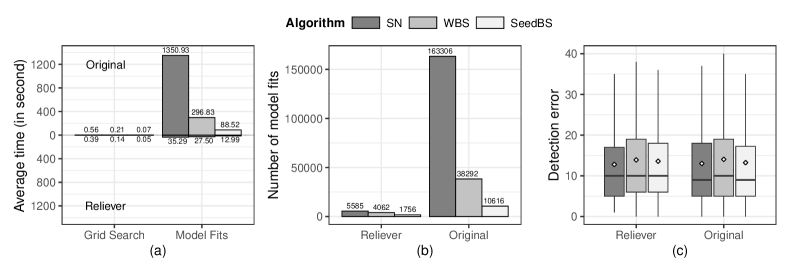
Figure 1.1: Comparison of computational efficiency and detection accuracy with and without Reliever for a high-dimensional linear model with multiple changepoints. The points in the boxplot represent the mean value.

1.2 Related Works

Most greedy grid search algorithms aim to alleviate the computational burden in changepoint detection by narrowing down the search space, which reduces the cardinality of $\mathcal{I}$. By doing so, these algorithms indirectly reduce the number of model fits. In contrast, our approach directly addresses the reduction of model fits. This strategy is particularly beneficial when the computational cost of fitting a model is high, as it often dominates the overall loss evaluations.

Our use of deterministic intervals is inspired by the concept of seeded intervals proposed by Kovács et al. (2022). In their work, the authors suggested replacing random intervals in the WBS algorithm with seeded intervals to achieve near-linear scaling of the number of loss evaluations with the sample size. However, the number of model fits could still be large, as a complete search for the best split within each seeded interval is required. Kovács et al. (2020) further proposed an optimistic search strategy that adaptively determines the best split within an interval instead of performing a complete search and paired this approach with the SeedBS algorithm for detecting multiple changepoints. In contrast, our approach utilizes deterministic intervals (i.e., relief intervals) to replace every search interval for model fitting (while the loss is still evaluated for that search interval). The reduction in the number of such intervals directly leads to computational speed-up. It is important to note that the design of relief intervals differs significantly from that of seeded intervals due to disparate objectives. For a more detailed discussion, please refer to Section 2.2.

Our approach of reducing heavy model fits is also related to the two-step procedures that utilize a preliminary set of changepoint candidates. In the context of high-dimensional linear models with a single changepoint, Kaul et al. (2019b) proposed a method that fits two regression models before and after an initial changepoint estimator and then searches for the best split to minimize the training error. The two fitted models are used for data before and after a candidate split. To achieve near-optimal convergence rates of the changepoint update, the initial changepoint estimator needs to be consistent. For multiple changepoint detection, Kaul et al. (2019a) extended this approach by initializing with multiple changepoint candidates and developing a simulated annealing algorithm to allocate available model fits. However, this method assumes that all true changepoints are located near some of the initial candidates. Similarly, in the context of univariate mean change models, Lu et al. (2017) proposed a method that uses a sparse subsample to obtain pilot changepoint estimators and then updates these estimators by sampling densely in neighborhoods around them. The pilot estimators need to be consistent in both the number and their locations of changepoints to obtain optimal changepoint estimators. Distinct from those works, our new proposal does not require consistent initial estimators and has general applicability, serving as a building block for existing changepoint detection algorithms.

1.3 Notations

The $L_{q}$ norm of a vector $\mathbf{z}\in\mathbb{R}^{p}$ is denoted as $\lVert\mathbf{z}\rVert_{q}=(\sum_{j=1}^{p}z_{j}^{q})^{1/q}$. The sub-Gaussian norm of a sub-Gaussian random variable $X$ is defined as $\|X\|_{\Psi_{2}}=\inf\{t>0:\mathbb{E}\{\exp(X^{2}/t^{2})\}\leq 2\}$. For $\bm{X}\in\mathbb{R}^{p}$, we define $\|\bm{X}\|_{\Psi_{2}}=\sup_{\bm{v}\in\mathbb{S}^{p-1}}\|\bm{v}^{\top}\bm{X}\|_{\Psi_{2}}$, where $\mathbb{S}^{p-1}$ represents the unit sphere. Let

$$\mathcal{T}_{K}(\delta_{m})=\{(\tau_{1},\ldots,\tau_{K}):0\equiv\tau_{0}<\tau_{1}<\cdots<\tau_{K}<\tau_{K+1}\equiv n,\tau_{k}-\tau_{k-1}\geq\delta_{m},\ k=1,\ldots,K+1\}$$

be a set of $K$ ordered integers with a minimal spacing $\delta_{m}>0$.

2 Methodology

2.1 The Changepoint Model and Grid Search Algorithms

Suppose we observe $\{\mathbf{z}_{i}\}_{i=1}^{n}$ from a multiple changepoint model

$$\mathbf{z}_{i}\sim\mathcal{M}_{k}^{\ast},\ \tau_{k-1}^{\ast}<i\leq\tau_{k}^{\ast},\ k=1,\ldots,K^{\ast}+1;\ i=1,\ldots,n,$$ (2.1)

where $K^{\ast}$ and $\{\tau_{k}^{\ast}\}$ denote the number and locations of changepoints, respectively, with the convention that $\tau_{0}^{\ast}=0$ and $\tau_{K^{\ast}+1}^{\ast}=n$. The notations $\{\mathcal{M}_{k}^{\ast}\}$ refer to the underlying models, where $\mathcal{M}_{k-1}^{\ast}\neq\mathcal{M}_{k}^{\ast}$. These models can represent either generally unknown distributions of $\{\mathbf{z}_{i}\}$ or specific parametric models such that $\mathcal{M}_{k}^{\ast}=\mathcal{M}_{\bm{\theta}_{k}^{\ast}}$ for a known model $\mathcal{M}$ and a sequence of unknown parameters of interest $\{\bm{\theta}_{k}^{\ast}\}$ satisfying $\bm{\theta}_{k-1}^{\ast}\neq\bm{\theta}_{k}^{\ast}$. A concrete example of such a model is the linear model with structural breaks (Bai and Perron, 1998), where we have paired observations $\{\mathbf{z}_{i}=(y_{i},\mathbf{x}_{i})\}_{i=1}^{n}$ with responses $y_{i}\in\mathbb{R}$ and covariates $\mathbf{x}_{i}\in\mathbb{R}^{p}$, admitting $y_{i}=\mathbf{x}_{i}^{\top}\bm{\theta}_{k}^{\ast}+\epsilon_{i}$, where $\{\bm{\theta}_{k}^{\ast}\}$ and $\{\epsilon_{i}\}$ are the regression coefficients and random noises, respectively.

We introduce a model fitting procedure that yields a fitted model $\widehat{\mathcal{M}}_{I}$ (or $\mathcal{M}_{\widehat{\theta}_{I}}$ in the case of parametric scenarios) based on the data $\{\mathbf{z}_{i}:i\in I\}$ within a specific interval $I\subset(0,n]$, e.g., the LASSO in situations where the linear model involves a large number of covariates. Following the model fitting step, we evaluate the quality of the fit by the loss function $\mathcal{L}(I;\widehat{\mathcal{M}}_{I})$ (or $\mathcal{L}(I;\widehat{\theta}_{I})$ in the parametric case), for the given interval $I$. Typically, the loss $\mathcal{L}$ is defined as the negative log-likelihood or least-squares loss for parametric models. A grid search algorithm is then employed to minimize a specific criterion over all possible segmented data sequences. This criterion typically comprises the sum of losses evaluated for each segment, along with a penalty that accounts for the complexity of the segmentation. Specially, consider a set of candidate changepoints $(\tau_{1},\ldots,\tau_{K})\in\mathcal{T}_{K}(\delta_{m})$ which partitions the data into $K+1$ segments, and the criterion is generally formed as

$$\sum_{k=1}^{K+1}\mathcal{L}((\tau_{k-1},\tau_{k}];\widehat{\mathcal{M}}_{k})+\gamma K,$$ (2.2)

where $\gamma\geq 0$ controls the level of penalization to prevent overestimation. Optimal-kind algorithms, such as the SN, OP, or PELT algorithm mentioned in Section 1, aim to find the exact minimizer over the entire search space $\mathcal{T}_{K}(\delta_{m})$. This involves evaluating a sequence of losses (along with fitting the corresponding models) for all $O(n^{2})$ intervals $I\subset(0,n]$ satisfying $|I|\geq\delta_{m}$, which are explored sequentially using a dynamic programming scheme. Although the PELT algorithm utilizes a pruning strategy to skip certain intervals and reduce its complexity to $O(n)$, this does not always apply (see Eq. (4) in Killick et al. (2012)). In contrast, greedy-kind algorithms, such as binary segmentation (BS), WBS, narrowest-over-threshold, or SeedBS algorithm, only consider a subset of these intervals $I$ in a sequential and greedy manner, aiming to reach a local minimizer. To illustrate, consider the BS algorithm. This algorithm begins by solving (2.2) with $K=1$, which involves approximately $O(n)$ intervals. The resulting changepoint divides the data sequence into two segments. Next, the algorithm applies the same procedure within each segment to identify new changepoints. This iterative process continues until a segment contains fewer observations than $\delta_{m}$ or a stopping rule is triggered. Overall, the BS algorithm requires evaluating approximately $O(n\log n)$ intervals. The intervals that are sequentially considered in the search path, whether using a global or greedy grid search algorithm, are referred to as search intervals. We can represent a grid search algorithm by $\mathcal{A}:=\mathcal{A}(\{\mathcal{L}(I;\widehat{\mathcal{M}}_{I})\}_{I\in\mathcal{I}})$, where $\mathcal{I}$ denotes the set of all search intervals.

2.2 Relief Intervals

Obtaining all model fits $\{\widehat{\mathcal{M}}_{I}\}_{I\in\mathcal{I}}$ along the search path can be computationally demanding, particularly when dealing with expensive-to-fit models. Our approach is straightforward yet versatile, and it can be used in conjunction with any grid search algorithm $\mathcal{A}=\mathcal{A}(\{\mathcal{L}(I;\widehat{\mathcal{M}}_{I})\}_{I\in\mathcal{I}})$. We begin by constructing a set of deterministic intervals $\mathcal{R}$. During the search process, for each search interval $I\in\mathcal{I}$, we employ a proxy or relief model $\widehat{\mathcal{M}}_{R}$ fitted using data from an interval $R\in\mathcal{R}$ to replace $\widehat{\mathcal{M}}_{I}$ when evaluating the loss $\mathcal{L}(I;\widehat{\mathcal{M}}_{I})$. The intervals $R\in\mathcal{R}$ are referred to as relief intervals to distinguish them from search intervals $I\in\mathcal{I}$. It is possible for multiple search intervals to correspond to a single relief interval, and not all relief intervals may be visited during the search. The key to this construction lies in satisfying two properties: first, significantly reducing the number of intervals for which a sequence of models needs to be fitted compared to considering all search intervals, and second, ensuring that the corresponding losses exhibit similar behavior to the original losses, allowing for the successful recovery of consistent changepoint estimators.

Definition 2.1 (Relief intervals).

Let $\delta_{m}>0$ represent the minimum length required between two successive candidate changepoints in a grid search algorithm. Let $0<w\leq 1$ be the wriggle parameter and $b>1$ be the growth parameter. For $0\leq k\leq\lfloor\log_{b}\{(1+w)n/\delta_{m}\}\rfloor$, define the $k$th layer as the collection of $n_{k}$ intervals of length $\ell_{k}$ that are evenly shifted by $s_{k}$ as $\mathcal{R}_{k}=\Bigl{\{}\Bigl{(}qs_{k},qs_{k}+\ell_{k}\Bigr{]}+a_{k}:0\leq q\leq n_{k}\Bigr{\}}$ and their collection $\mathcal{R}=\bigcup_{k=0}^{\lfloor\log_{b}\{(1+w)n/\delta_{m}\}\rfloor}\mathcal{R}_{k}$ as the set of relief intervals, where $\ell_{k}=b^{k}\delta_{m}/(1+w)$, $s_{k}=w\ell_{k}$, $n_{k}=\lfloor(n-\ell_{k})/s_{k}\rfloor$, and $a_{k}=n/2-(\ell_{k}+n_{k}s_{k})/2$ is an adjustment factor to center the intervals in $\mathcal{R}_{k}$ around $n/2$.

Figure 2.1: Construction of relief intervals with $n=200,\delta_{m}=50,w=0.25$ and $b=1.25$.

In Figure 2.1, we provide an illustration of the construction of relief intervals with $n=200$, $\delta_{m}=50$, $w=0.25$, and $b=1.25$. The rationale behind this construction is to ensure that for any search interval $I\in\mathcal{I}$ with $|I|\geq\delta_{m}$, we can always find a relief interval $R\in\mathcal{R}$ such that $R\subset I$ and $|R|/|I|$ is maximized. We define the coverage rate as $r=\min_{I\in\mathcal{I}:|I|\geq\delta_{m}}\max_{R\in\mathcal{R};R\subset I}|R|/|I|$.

Proposition 2.1.

(i) $|\mathcal{R}|\leq c_{w,b}n/\delta_{m}$ and $r\geq\{(1+w)b\}^{-1}$, where $c_{w,b}=\{(1+w)b\}/\{w(b-1)\}$.

(ii) If we set $\delta_{m}=C\log n$ for some constant $C>0$ and $w=b-1=\delta_{m}^{-1/2}$, then $|\mathcal{R}|\leq n\{1+(C\log n)^{-1/2}\}^{2}=O(n)$ and $r\geq\{1+(C\log n)^{-1/2}\}^{-2}\approx 1-2(C\log n)^{-1/2}$.

Proposition 2.1 demonstrates that, by selecting appropriate wriggle and growth parameters along with the minimal search distance, the number of relief intervals approaches linearity in the sample size $n$ while achieving a nearly perfect coverage rate. In practical applications, we can set a coverage parameter $r\in(0,1)$ and let $1+w=b=r^{-1/2}$. The $r$ acts as a tuning parameter that balances computational complexity and estimation accuracy. Table 2.1 displays the number of search intervals obtained from a complete search over all intervals with a minimum length of $\delta_{m}=30$ for $n=1200$, as well as the number of relief intervals corresponding to different coverage parameters $r$. In practice, we recommend selecting $r\in[0.8,0.9]$, as it significantly reduces computational time while producing satisfactory performances compared to the original implementation.

Table 2.1: The number of relief intervals across the coverage parameter $r$ for $(n,\delta_{m})=(1200,30)$.

Complete search	Reliever with coverage $r$
	0.5	0.6	0.7	0.8	0.9	0.95	0.97	0.99
686206	440	762	1298	2744	12227	31699	57522	196395

Remark.

The deterministic nature of our relief intervals is inspired by the concept of seeded intervals introduced by Kovács et al. (2022). They proposed replacing random intervals in the WBS algorithm and its variants with deterministic intervals. Their approach focused on constructing shorter intervals that contain a single changepoint, thereby reducing the occurrence of longer intervals that may contain multiple changepoints. In contrast, our approach is applicable to a wide range of grid search algorithms beyond WBS. We construct deterministic intervals to replace all search intervals that enter the search path, ensuring that each search interval approximately covers a relief interval.

2.3 The Reliever Procedure

• Require a gird search algorithm $\mathcal{A}=\mathcal{A}(\{\mathcal{L}(I;\widehat{\mathcal{M}}_{I})\})$ with a minimal search distance $\delta_{m}\geq 0$ and a model fitting procedure $\widehat{\mathcal{M}}_{I}$ for any interval $I$ such that $|I|\geq\delta_{m}$, and a coverage parameter $r\in(0,1)$;

• Create a collection of relief intervals $\mathcal{R}$ according to Definition 2.1 with the wriggle and growth parameters $1+w=b=r^{-1/2}$;

• Apply the gird search algorithm with relief models, i.e., $\mathcal{A}=\mathcal{A}(\{\mathcal{L}(I;\widehat{\mathcal{M}}_{R})\})$ with $R=\operatorname*{\mathrm{arg\,max}}\nolimits_{R\in\mathcal{R},R\subset I}|R|$.

The Reliever procedure can be utilized in conjunction with both optimal- and greedy-kind grid search algorithms that can be represented as $\mathcal{A}=\mathcal{A}(\{\mathcal{L}(I;\widehat{\mathcal{M}}_{I})\})$. When employing the Reliever approach, the only difference from the original implementation lies in the employment of a relief model $\widehat{\mathcal{M}}_{R}$ to evaluate the loss function $\mathcal{L}(I;\cdot)$. This key characteristic renders Reliever highly versatile. By constructing relief intervals $\mathcal{R}$, the number of model fits required in the Reliever procedure can be bounded by $O(n)$, resulting in a significant reduction compared to the original implementation (see Table 1.1).

3 Theoretical Justifications

Despite the applicability of Reliever to various detection algorithms and model settings, establishing a unified theoretical framework for analyzing detection accuracy is challenging without specific assumptions regarding the involved model, fitting algorithm, and grid search algorithm. Here, we first offer an informal justification by examining the variations in loss values resulting from the application of the Reliever technique. Additionally, in Section 3.1, we present rigorous results on changepoints estimation for a concrete example involving high-dimensional linear regression models.

We focus on parametric change detection using loss functions $\mathcal{L}(I;\bm{\theta}_{I})=\sum_{i\in I}\ell(\mathbf{z}_{i},\bm{\theta}_{I})$, where $\ell(\cdot,\bm{\theta})$ is a convex function with respect to the parameter $\bm{\theta}\in\Theta\subset\mathbb{R}^{p}$. We consider the small-$p$-and-large-$n$ scenario. For the model-fitting module, we utilize the M-estimator, which estimates the parameter as $\widehat{\bm{\theta}}_{I}=\operatorname*{\mathrm{arg\,min}}_{\bm{\theta}\in\Theta}\sum_{i\in I}\ell(\mathbf{z}_{i},\bm{\theta})$. The corresponding population version is defined as $\bm{\theta}_{I}^{\circ}=\operatorname*{\mathrm{arg\,min}}_{\bm{\theta}\in\Theta}\sum_{i\in I}\mathbb{E}\{\ell(\mathbf{z}_{i},\bm{\theta})\}$. In the original implementation of a grid search algorithm $\mathcal{A}$, the losses $\mathcal{L}(I,\widehat{\bm{\theta}}_{I})=\sum_{i\in I}\ell(\mathbf{z}_{i},\widehat{\bm{\theta}}_{I})$ are evaluated. With the Reliever approach, these losses are replaced by $\mathcal{L}(I,\widehat{\bm{\theta}}_{R})=\sum_{i\in I}\ell(\mathbf{z}_{i},\widehat{\bm{\theta}}_{R})$, where $R\in\mathcal{R}$ represents a relif interval corresponding to $I$ such that $R\subset I$. Theorem 3.1 establishes the distinction between the losses $\mathcal{L}(I,\widehat{\bm{\theta}}_{I})$ and $\mathcal{L}(I,\widehat{\bm{\theta}}_{R})$ uniformly across all intervals $I\subset(0,n]$.

Theorem 3.1.

Given that the conditions outlined in Appendix A are satisfied. With probability at least $1-n^{-C}$ for some constant $C>0$, the event

$$0\leq\frac{1}{|I|}\{\mathcal{L}(I,\widehat{\bm{\theta}}_{R})-\mathcal{L}(I,\widehat{\bm{\theta}}_{I})\}\leq O\biggl{(}\biggl{\lVert}\frac{1}{|I|}\sum_{i\in I\setminus R}\mathbb{E}\nabla_{\bm{\theta}}\ell(\mathbf{z}_{i},\bm{\theta}_{R}^{\circ})\biggr{\rVert}_{2}^{2}+(1-r)\frac{\log n}{|I|}+\frac{(\log n)^{2}}{|I|^{2}}\biggr{)}$$ (3.1)

holds uniformly for all intervals $R\subset I\subset(0,n]$, where $\nabla_{\bm{\theta}}\ell(\cdot,\bm{\theta})$ denotes the gradient or sub-gradient. Moreover, for the cases where either $I=(s,e]$ contains no changepoint or there is only one changepoint $\tau\in I$ such that $\min(\tau-s,e-\tau)=O(\log n)$, this event simplifies to

$$0\leq\frac{1}{|I|}\{\mathcal{L}(I,\widehat{\bm{\theta}}_{R})-\mathcal{L}(I,\widehat{\bm{\theta}}_{I})\}\leq C_{1}\biggl{(}(1-r)\frac{\log n}{|I|}+\frac{(\log n)^{2}}{|I|^{2}}\biggr{)},$$ (3.2)

where $C_{1}>0$ is a constant.

Remark.

The conditions in Appendix A bear similarities to those presented in Niemiro (1992), which focused on the asymptotic properties of M-estimators obtained through convex minimization based on independent and identically distributed (i.i.d.) data sequence. These conditions primarily impose requirements on the smoothness and convexity of the loss function $\ell$ and its expectation. The proof of Theorem 3.1 relies on a novel non-asymptotic Bahadur-type representation of $\widehat{\bm{\beta}}_{I}-\widehat{\bm{\beta}}_{R}$ in the presence of changepoints across all sub-intervals $I\subset(0,n]$.

In Theorem 3.1, Eq. (3.2) indicates that the discrepancy between a Reliever-based loss $\mathcal{L}(I,\widehat{\bm{\theta}}_{R})$ and its original counterpart $\mathcal{L}(I,\widehat{\bm{\theta}}_{I})$ vanishes when the data within $I$ are (nearly) homogeneous and $\log n/|I|\rightarrow 0$, which provides a justification for the use of of Reliever. However, for heterogeneous $I$ that contains a changepoint located far from the boundaries, this vanishing property is not ensured. Surprisingly, the inequality $\mathcal{L}(I,\widehat{\bm{\theta}}_{R})\geq\mathcal{L}(I,\widehat{\bm{\theta}}_{I})$ in Eq. (3.1) becomes valuable in excluding inconsistent changepoint estimators in these cases. Therefore, we can expect that Reliever can effectively track the original search path. To gain some intuition, consider a scenario where there is a single changepoint $\tau^{\ast}$ such that $\min(\tau^{\ast},n-\tau^{\ast})\geq\delta_{m}$ or $\tau^{\ast}\in\mathcal{T}_{1}(\delta_{m})$. We specify the grid search algorithm as the first step of the BS procedure and define the changepoint estimator as $\widehat{\tau}_{\mathrm{original}}=\operatorname*{\mathrm{arg\,min}}_{\tau\in\mathcal{T}_{1}(\delta_{m})}S^{(I)}_{I}(\tau)$, where $S^{(I)}_{I}(\tau)=\mathcal{L}(I_{1,\tau},\widehat{\bm{\theta}}_{I_{1,\tau}})+\mathcal{L}(I_{2,\tau},\widehat{\bm{\theta}}_{I_{2,\tau}})$, and for any $\tau$, $I_{1,\tau}=(0,\tau]$ and $I_{2,\tau}=(\tau,n]$. The Reliever-based changepoint estimator is denoted as $\widehat{\tau}=\operatorname*{\mathrm{arg\,min}}_{\tau\in\mathcal{T}_{1}(\delta_{m})}S^{(R)}_{I}(\tau)$, where $S^{(R)}_{I}(\tau)=\mathcal{L}(I_{1,\tau},\widehat{\bm{\theta}}_{R_{1,\tau}})+\mathcal{L}(I_{2,\tau},\widehat{\bm{\theta}}_{R_{2,\tau}})$, and $R_{j,\tau}\subset I_{j,\tau}$ is the corresponding relief interval for $j=1,2$. We present the following corollary which establishes the consistency of $\widehat{\tau}$.

Corollary 3.2.

Assume $\delta_{m}=C_{m}\log n$ for some constant $C_{m}>0$, and the event described in Theorem 3.1 holds. If there exists a sufficiently large constant $C_{2}>0$ such that for any $\tau\in\mathcal{T}_{1}(\delta_{m})$ satisfying $|\tau-\tau^{\ast}|>\delta$ for a constant $\delta>0$,

$$S^{(I)}_{I}(\tau)-S^{(I)}_{I}(\tau^{\ast})>C_{2}\log n$$ (3.3)

holds, then $|\widehat{\tau}-\tau^{\ast}|\leq\delta$.

Corollary 3.2 is a direct consequence of Theorem 3.1. Assume $|\widehat{\tau}-\tau^{\ast}|>\delta$. Since $\mathcal{L}(I,\widehat{\bm{\theta}}_{R})\leq\mathcal{L}(I,\widehat{\bm{\theta}}_{I})$ according to Eq. (3.1), it implies that $S^{(R)}_{I}(\widehat{\tau})\geq S^{(I)}_{I}(\widehat{\tau})$. By utilizing Eq. (3.2), we can derive

$$S^{(R)}_{I}(\tau^{\ast})\leq S^{(I)}_{I}(\tau^{\ast})+2C_{1}\Big{\{}(1-r)+\frac{n\log n}{\tau^{\ast}(n-\tau^{\ast})}\Big{\}}\log n.$$

Considering Eq. (3.3), we have $S^{(R)}_{I}(\widehat{\tau})-S^{(R)}_{I}(\tau^{\ast})>C_{2}\log n-2C_{1}\Big{\{}(1-r)+C_{m}^{-1}\Big{\}}\log n\geq 0$, by selecting $C_{2}\geq 2C_{1}\{(1-r)+C_{m}^{-1}\}$. Therefore, the assumption $|\widehat{\tau}-\tau^{\ast}|>\delta$ leads to a contradiction, consequently establishing the validity of Corollary 3.2. Eq. (3.3) imposes implicit constraints on the model, ensuring that the original grid search algorithm produces a consistent changepoint estimator, i.e., $|\widehat{\tau}_{\mathrm{original}}-\tau^{\ast}|\leq\delta$. The verification of Eq. (3.3) or the establishment of a lower bound for $S^{(I)}_{I}(\tau)-S^{(I)}_{I}(\tau^{\ast})$ is a widely accepted technique for justifying the consistency of changepoint estimators (Csörgő and Horváth, 1997). Corollary 3.2 demonstrates that the consistency proof for the original grid search algorithm can readily be extended to the Reliever estimator.

3.1 High-dimensional Linear Models with Changepoints

To gain a comprehensive understanding of how variations in loss functions impact the accuracy of changepoint detection using the Reliever device, we investigate the problem of detecting multiple changepoints in high-dimensional linear models, which has recently garnered considerable attention (Leonardi and Bühlmann, 2016; Kaul et al., 2019a; Rinaldo et al., 2021; Wang et al., 2021b; Xu et al., 2022). In our study, the data consists of independent pairs of response and covariates, denoted as $(y_{i},\mathbf{x}_{i})\in\mathbb{R}\times\mathbb{R}^{p}$, satisfying

$$y_{i}=\mathbf{x}_{i}^{\top}\bm{\beta}_{k}^{\ast}+\epsilon_{i},\ \tau_{k-1}^{\ast}<i\leq\tau_{k}^{\ast},\ k=1,\ldots,K^{\ast}+1;\ i=1,\ldots,n.$$ (3.4)

Here, $\{\bm{\beta}_{k}^{\ast}\}$ represent the regression coefficients, and $\{\epsilon_{i}\}$ denote the random noises. Our objective is to identify the unknown number of changepoints $K^{\ast}$ and their corresponding locations $\{\tau_{k}^{\ast}\}$ from the observed data. We take a conventional high-dimensional regime where both $n$ and $p$ diverge, and focus on the case of sparse regression coefficients.

We adopt the OP algorithm for detecting multiple changepoints, as proposed by Leonardi and Bühlmann (2016). We utilize the LASSO procedure to estimate the regression coefficients within a given interval $I\subset(0,n]$ with $|I|\geq\delta_{m}$. The estimated coefficients, denoted as $\widehat{\bm{\beta}}_{I}$, are obtained by solving

$$\widehat{\bm{\beta}}_{I}=\operatorname*{\mathrm{arg\,min}}_{\bm{\beta}\in\mathbb{R}^{p}}\{\mathcal{L}(I;\bm{\beta})+\lambda_{I}\lVert\bm{\beta}\rVert_{1}\},$$

where $\mathcal{L}(I;\bm{\beta})=\sum_{i\in I}(y_{i}-\mathbf{x}_{i}^{\top}\bm{\beta})^{2}$ represents the loss function for the interval $I$, and $\lambda_{I}$ is a tuning parameter that promotes sparsity in the estimated coefficients. The original implementation of the OP algorithm involves minimizing the criterion

$$\sum_{k=1}^{K+1}\mathcal{L}((\tau_{k-1},\tau_{k}];\widehat{\bm{\beta}}_{(\tau_{k-1},\tau_{k}]})+\gamma K,$$ (3.5)

over all candidate changepoints $(\tau_{1},\ldots,\tau_{K})\in\mathcal{T}_{K}(\delta_{m})$. Here, $\gamma$ is an additional tuning parameter that discourages overestimation of the number of changepoints. The specific values of $\lambda_{I}$ and $\gamma$ will be specified later in our theoretical analysis. To incorporate the Reliever procedure into the OP algorithm, as outlined in Section 2.3, we construct a collection of relief intervals $\mathcal{R}$ with a coverage parameter $0<r<1$. The criterion to be minimized then becomes

$$\sum_{k=1}^{K+1}\mathcal{L}((\tau_{k-1},\tau_{k}];\widehat{\bm{\beta}}_{R_{k}})+\gamma K,\mbox{ with }R_{k}=\operatorname*{\mathrm{arg\,max}}\nolimits_{R\in\mathcal{R},R\subset(\tau_{k-1},\tau_{k}]}|R|.$$ (3.6)

The optimization problems (3.5) and (3.6) can indeed be regarded as special cases of a more general optimization problem

$$\min_{(\tau_{1},\ldots,\tau_{K})\in\mathcal{T}_{K}(\delta_{m})}\left\{\sum_{k=1}^{K+1}\mathcal{L}\Big{(}(\tau_{k-1},\tau_{k}];\widetilde{\bm{\beta}}\big{(}(\tau_{k-1},\tau_{k}]\big{)}\Big{)}+\gamma K\right\}.$$ (3.7)

Here, $\widetilde{\bm{\beta}}(I)$ can represent any valid estimator of the regression coefficients within an interval $I$ such that $|I|\geq\delta_{m}$. By setting $\widetilde{\bm{\beta}}(I)=\widehat{\bm{\beta}}_{I}$, we can recover (3.5). Similarly, if we choose $\widetilde{\bm{\beta}}(I)=\widehat{\bm{\beta}}_{R_{I}}$ with $R_{I}=\operatorname*{\mathrm{arg\,max}}\nolimits_{R\in\mathcal{R},R\subset I}|R|$, we obtain the problem (3.6). The optimization (3.7) can be addressed using the OP algorithm, which integrates a sequence of parameter estimation and loss evaluation steps along the search path, i.e., $\{\mathcal{L}_{I}\equiv\mathcal{L}(I;\widetilde{\bm{\beta}}(I)):I\subset(0,n],|I|\geq\delta_{m}\}$. The dynamic ordering of the intervals $I$ is determined by the OP algorithm itself.

We first state a deterministic claim regarding the consistency and near rate-optimality of the resulting changepoint estimators, but conditional on an event measuring the goodness of the solution path. To this end, we introduce some notations and conditions. For any interval $I\subset(0,n]$, denote $\bm{\beta}_{I}^{\circ}=\operatorname*{\mathrm{arg\,min}}_{\bm{\beta}\in\mathbb{R}^{p}}\mathbb{E}\{\mathcal{L}(I;\bm{\beta})\}$, and define $\Delta_{I}=({|I|}^{-1}\sum_{i\in I}\lVert\bm{\beta}_{i}^{\circ}-\bm{\beta}_{I}^{\circ}\rVert_{\Sigma}^{2})^{1/2}$, where $\bm{\beta}_{i}^{\circ}=\bm{\beta}_{\{i\}}^{\circ}$ for $i=1,\ldots,n$. For $k=1,\ldots,K^{\ast}$, let $\Delta_{k}=\lVert\bm{\beta}_{k+1}^{\ast}-\bm{\beta}_{k}^{\ast}\rVert_{\Sigma}$ be the change magnitude at $\tau_{k}^{\ast}$, and we extend the definition to $\Delta_{0}=\Delta_{K^{\ast}+1}=\infty$.

Condition 3.1 (Change signals).

There exists a sufficiently large constant $C_{\mathsf{snr}}>0$ such that for $k=1,\dots,K^{\ast}+1$, $\tau_{k}^{\ast}-\tau_{k-1}^{\ast}\geq C_{\mathsf{snr}}s\log(p\vee n)(\Delta_{k-1}^{-2}\vee 1+\Delta_{k}^{-2}\vee 1)$.

Condition 3.2 (Regression coefficients).

(a) Sparsity: $|\mathcal{S}_{k}|\leq s<p$, where $\mathcal{S}_{k}=\{1\leq j\leq p:\beta_{k,j}^{\ast}\neq 0\}$ and $\beta_{k,j}^{\ast}$ is the $j$th component of $\bm{\beta}_{k}^{\ast}$; (b) Boundness: $|\beta_{k,j}^{\ast}|\leq C_{\beta}$ for some constant $C_{\beta}>0$.

Condition 3.3 (Covariates and noises).

(a) $\{\mathbf{x}_{i}\}_{i=1}^{n}$ are i.i.d. with a sub-Gaussian distribution, having zero mean and covariance $\Sigma$. The $\Sigma$ satisfies that $0<\underline{\kappa}\leq\sigma_{x}^{2}<\infty$, where $\underline{\kappa}=\lambda_{\min}(\Sigma)$ and $\sigma_{x}^{2}=\lambda_{\max}(\Sigma)$ are the minimum and maximum eigenvalues of $\Sigma$, respectively. Furthermore, $\lVert\Sigma^{-1/2}\mathbf{x}_{i}\rVert_{\Psi_{2}}\leq C_{x}$ for some constant $C_{x}>0$; (b) $\{\epsilon_{i}\}_{i=1}^{n}$ are i.i.d. with a sub-Gaussian distribution, having zero mean, variance $\sigma_{\epsilon}^{2}$, and sub-Gaussian norm $C_{\epsilon}$.

These conditions are commonly adopted in the literature for multiple changepoint detection in high-dimensional linear models (Leonardi and Bühlmann, 2016; Wang et al., 2021b; Rinaldo et al., 2021; Xu et al., 2022). Specifically, Condition 3.1 introduces a local multiscale signal-to-noise ratio (SNR) requirement for the spacing between neighboring changepoints, providing greater flexibility compared to the global SNR condition in existing works like Leonardi and Bühlmann (2016) and Wang et al. (2021b).

Lemma 3.3.

Given that Condition 3.1 is satisfied. The solution $(\widehat{\tau}_{1},\ldots,\widehat{\tau}_{\widehat{K}})$ of the optimization problem (3.7) with $\delta_{m}=C_{m}s\log(p\vee n)$ for a sufficiently large constant $C_{m}>0$, and $\gamma=C_{\gamma}s\log(p\vee n)$ for a constant $C_{\gamma}>0$, satisfies that

$$\widehat{K}=K^{\ast}\mbox{ and }\max_{1\leq k\leq K^{\ast}}\min_{1\leq j\leq\widehat{K}}\frac{1}{2}\Delta_{k}^{2}|\tau_{k}^{\ast}-\widehat{\tau}_{j}|\leq\widetilde{C}s\log(p\vee n),$$

for some constant $\widetilde{C}>0$, conditional on the event $\mathbb{G}=\mathbb{G}_{1}\cap\mathbb{G}_{2}\cap\mathbb{G}_{3}$. Here,

$$\mathbb{G}_{1} =\left\{\mbox{for any }I\in E_{1},\Bigl{|}\mathcal{L}_{I}-\sum_{i\in I}\epsilon_{i}^{2}\Bigr{|}<C_{\ref*{lem:loc_err_g}.1}s\log(p\vee n)\right\},$$

$$\mathbb{G}_{2} =\left\{\mbox{for any }I\in E_{2},\Bigl{|}\mathcal{L}_{I}-\sum_{i\in I}\epsilon_{i}^{2}-\Delta_{I}^{2}|I|\Bigr{|}<C_{\ref*{lem:loc_err_g}.2}s\log(p\vee n)\right\},$$

$$\mathbb{G}_{3} =\left\{\mbox{for any }I\in E_{3},\mathcal{L}_{I}-\sum_{i\in I}\epsilon_{i}^{2}>(1-C_{\ref*{lem:loc_err_g}.3})\Delta_{I}^{2}|I|\right\},$$

with $E_{1}=\{I:\Delta_{I}=0\}$, $E_{2}=\{I:0<\Delta_{I}^{2}|I|\leq\widetilde{C}s\log(p\vee n),|I\cap\mathcal{T}^{\ast}|\leq 1\}$and $E_{3}=\{I:\Delta_{I}^{2}|I|\geq\widetilde{C}s\log(p\vee n)\}$, and $C_{\ref*{lem:loc_err_g}.1}$, $C_{\ref*{lem:loc_err_g}.2}$ and $C_{\ref*{lem:loc_err_g}.3}$ are positive constants. In addition, the constants $C_{\gamma}$ and $\widetilde{C}$ only depends on $C_{\mathsf{snr}}$, $C_{m}$, $C_{\ref*{lem:loc_err_g}.1}$, $C_{\ref*{lem:loc_err_g}.2}$, and $C_{\ref*{lem:loc_err_g}.3}$.

Lemma 3.3 is actually a deterministic result. The probabilistic conditions come into play when certifying that the event $\mathbb{G}$ holds with high probability for both the original implementation of the detection procedure with $\mathcal{L}_{I}=\mathcal{L}(I;\widehat{\bm{\beta}}_{I})$ and the accelerated version achieved through Reliever with $\mathcal{L}_{I}=\mathcal{L}(I;\widehat{\bm{\beta}}_{R_{I}})$. Lemma 3.3 offers new insights into the requirements for the solution path of the OP algorithm to produce consistent and nearly rate-optimal changepoint estimators, which may be of independent interest. Theorem 3.4 asserts that the event $\mathbb{G}$ occurs with high probability when additional Conditions 3.2–3.3 are satisfied.

Theorem 3.4.

Given that Conditions 3.1–3.3 are satisfied. Let $C_{\lambda}$ and $C_{\gamma}$ be positive constants, and $0<C_{m}<C_{\mathsf{snr}}$ be sufficiently large constants. The solution $(\widehat{\tau}_{1},\ldots,\widehat{\tau}_{\widehat{K}})$ of either Problem (3.5) or Problem (3.6) with $\delta_{m}=C_{m}s\log(p\vee n)$, $\lambda_{I}=C_{\lambda}C_{x}\sigma_{x}D_{I}\sqrt{|I|\log(p\vee n)}$, and $\gamma=C_{\gamma}s\log(p\vee n)$, satisfies that

$$\mathbb{P}\Bigl{\{}\widehat{K}=K^{\ast}\mbox{ and }\max_{1\leq k\leq K^{\ast}}\min_{1\leq j\leq\widehat{K}}\Delta_{k}^{2}|\tau_{k}^{\ast}-\widehat{\tau}_{j}|\leq\widetilde{C}s\log(p\vee n)\Bigr{\}}\geq 1-(p\vee n)^{-c},$$

where $D_{I}=\sqrt{C_{x}^{2}\Delta_{I}^{2}+C_{\epsilon}^{2}}$. The constants $C_{\gamma}$, $C_{\lambda}$, $\widetilde{C}$ and $c$ are independent of $(n,p,s,K^{\ast})$. Moreover, under the same event, there exists a constant $C>0$ such that for all $1\leq k\leq K^{\ast}+1$,

$$\lVert\widehat{\bm{\beta}}_{(\widehat{\tau}_{k-1},\widehat{\tau}_{k}]}-\bm{\beta}_{k}^{\ast}\rVert_{2}\leq C\sqrt{\frac{s\log(p\vee n)}{\tau_{k}^{\ast}-\tau_{k-1}^{\ast}}}.$$

Theorem 3.4 demonstrates that under mild conditions and by appropriately choosing the tuning parameters $\gamma$ and $\lambda_{I}$, both the original implementation of the OP algorithm (3.5) and its Reliever counterpart (3.6) consistently estimate the number of changepoints and achieve a state-of-the-art localization rate $|\tau_{k}^{\ast}-\widehat{\tau}_{k}|/n\leq C\Delta_{k}^{-2}s\log(p\vee n)/n$ with high probability. This localization rate exhibits the phenomenon of superconsistency for changepoint estimation in high-dimensional linear regression with multiple changepoints, extending a well-known result for single changepoint scenarios (Lee et al., 2016). Importantly, our analysis allows for $K^{*}$ to depend on $n$ and potentially diverge. When $K^{*}=O(1)$, the rate aligns with the findings in Rinaldo et al. (2021) and Xu et al. (2022), which employ OP-type algorithms. Wang et al. (2021b) allows for $K^{*}$ to diverge and derives this rate using a WBS-type algorithm. Additionally, it is noteworthy that the tuning parameter $\lambda_{I}$, which controls the level of penalization for the model within $I$, not only scales with $|I|^{1/2}$ but also depends on the change magnitude $\Delta_{I}^{2}$. In fact, determining the rate of $\lambda_{I}$ involves examining the uniform bound of a sequence of mean-zero (sub-)gradients, where the variance is, however, influenced by $\Delta_{I}^{2}$. When assuming that $\sup_{I}\Delta_{I}^{2}=O(1)$, as done in previous works (Wang et al., 2021b; Xu et al., 2022), this dependence disappears, and thus $\lambda_{I}$ specified in those works scales solely with $|I|^{1/2}$. Theorem 3.4 offers valuable insights into the selection of the nuisance parameter, highlighting its change-adaptive nature. Although the detailed exploration of this aspect is beyond the scope of our paper, it calls for further research and investigation.

Upon initial examination, it may seem that Reliever enjoys a free lunch, as the localization rate appears to be independent of the coverage rate $r$. However, with a closer inspection of the proof, it becomes apparent that the coverage rate $r$ is absorbed into the localization rate constant $\tilde{C}$ since $r$ is fixed. Specifically, the value of $\tilde{C}$ depends on the constants $C_{\mathsf{snr}}$, $C_{m}$, $C_{\ref*{lem:loc_err_g}.1}$, $C_{\ref*{lem:loc_err_g}.2}$, and $C_{\ref*{lem:loc_err_g}.3}$, as stated in Lemma 3.3. In fact, by choosing $C_{\mathsf{snr}}$ and $C_{m}$ sufficiently large, we have $\widetilde{C}=2(1-C_{\ref*{lem:loc_err_g}.3})^{-1}(3C_{\ref*{lem:loc_err_g}.1}+10C_{\ref*{lem:loc_err_g}.2})$. It can be shown that the constants $C_{\ref*{lem:loc_err_g}.j}$ for $j=1,2,3$ increase as $r$ decreases, resulting in an increase in $\tilde{C}$ with respect to $r$. In other words, smaller values of $r$ lead to worse localization rates. Therefore, the coverage rate $r$ in Reliever provides a trade-off between computational efficiency and localization accuracy, as anticipated. In the regime where $r\rightarrow 1$, one can expect that the difference between the Reliever and the original grid search algorithm would diminish. See Corollary C.11 in Supplementary Material for specific values of $C_{\ref*{lem:loc_err_g}.j}$, $j=1,2,3$.

4 Numerical Studies

To demonstrate the advantages of employing the Reliever approach in conjunction with various change detection algorithms, we examine three grid search algorithms: SN, WBS, and SeedBS. We evaluate each algorithm under both a high-dimensional linear model and a nonparametric model. For illustrative purposes, we fix the number of wild intervals $M=100$ for WBS, and set the decay parameter $a=1/\sqrt{2}$ for SeedBS as recommended in Kovács et al. (2022). All the results presented in Section 4 are based on $500$ replications.

4.1 High-dimensional Linear Regression Models

In the first scenario, we investigate the linear model (3.4) with $p=100$ and $n\in\{300,600,900,1200\}$. The covariates $\{\mathbf{x}_{i}\}$ are i.i.d. from the standard multivariate Gaussian distribution, and the noises $\{\epsilon_{i}\}$ are i.i.d. from the standard Gaussian distribution $\mathcal{N}(0,1)$. We introduce three changepoints $\{\tau_{k}^{\ast}\}_{k=1}^{3}=\{\lfloor 0.22n\rfloor,\lfloor 0.55n\rfloor,\lfloor 0.77n\rfloor\}$ into the model. The regression coefficients $\{\bm{\theta}_{k}^{\ast}\}$ are generated such that $\theta_{k,j}=0$ for $j=3,\ldots,p$, and $\theta_{k,1}$ and $\theta_{k,2}$ are uniformly sampled, satisfying the signal-to-noise ratios $\lVert\bm{\theta}_{1}\rVert_{2}/\sqrt{\operatorname*{\mathrm{Var}}\{\epsilon_{1}\}}=2$ and $\lVert\bm{\theta}_{k}-\bm{\theta}_{k-1}\rVert_{2}/\sqrt{\operatorname*{\mathrm{Var}}\{\epsilon_{1}\}}=1/2$ for $k=2,3,4$. Here $\theta_{k,j}$ denotes the $j$th element of $\bm{\theta}_{k}$. To estimate the sparse linear regression model, we utilize the glmnet package (Friedman et al., 2010) in R. We specify a set of hyperparameters $\{\lambda\}$, consisting of $30$ values, and for each search interval $I$, we set $\lambda_{I}=\lambda\sqrt{|I|}$. For a specific $\lambda$, we can apply any of the three grid search algorithms with the prior knowledge of the number of changepoints $K^{\ast}=3$. Across the entire set of hyperparameters $\{\lambda\}$, we report the smallest detection error measured by the Hausdorff distance between the estimated and true changepoints, i.e.

$$\max\Bigl{(}\max_{1\leq k\leq K^{\ast}}\min_{1\leq j\leq K^{\ast}}|\tau_{k}^{\ast}-\widehat{\tau}_{j}|,\max_{1\leq j\leq K^{\ast}}\min_{1\leq k\leq K^{\ast}}|\tau_{k}^{\ast}-\widehat{\tau}_{j}|\Bigr{)}.$$ (4.1)

Figures 4.1–4.2 display the detection error and computation time associated with different grid search algorithms at varying values of the coverage rate parameter $r$. Notice that $r=0.9$ represents the recommended value for the Reliever method, while $r=1$ corresponds to the original implementation of each respective algorithm. The results indicate that as the coverage rate parameter $r$ approaches $1$, the performance of the Reliever method converges to that of the original implementation. Furthermore, when $r=0.9$, the performance remains nearly identical to the original implementation, while achieving significant time savings. Even when $r=0.6$, the performance is still acceptable, considering the negligible running time.

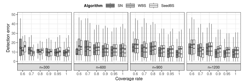
Figure 4.1: Detection error for SN, WBS and SeedBS algorithms across varying values of the coverage rate parameter, under the high-dimensional linear model.

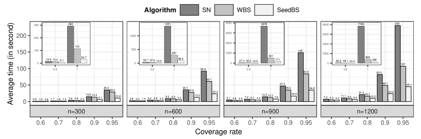
Figure 4.2: Computation time for SN, WBS and SeedBS algorithms across varying values of the coverage rate parameter, under the high-dimensional linear model.

4.2 Changepoint Detection in the Nonparametric Model

In the second scenario, we examine the nonparametric changepoint model (2.1), where the data $\{z_{i}\}_{i=1}^{n}$ follows the distribution

$$z_{i}\sim F_{k}(z),\ \tau_{k-1}^{\ast}<i\leq\tau_{k}^{\ast},\ k=1,\dots,K^{\ast}+1;\ i=1,\dots,n.$$

Here $F_{k}$ represents the cumulative distribution function (C.D.F.). Zou et al. (2014) proposed an NMCD method. This approach involves defining the loss function corresponding to a search interval as the integrated nonparametric maximum log-likelihood function, fitting the model using the empirical C.D.F. of the data within that interval, and employing the OP algorithm to search for multiple changepoints. Haynes et al. (2017) further enhanced the computational efficiency by discretizing the integral and applying the PELT algorithm. To reduce the computational cost of fitting the model, which involves approximating the integral and can be computationally intensive, we leverage the Reliever method. Instead of using the empirical C.D.F. for the search interval, we replace it with its Reliever counterpart, constructed based on data within a relief interval. In this scenario, we consider the same three-changepoint setting as in the first scenario. The data for the four segments are generated from four different distributions, i.e., $\mathcal{N}(0,1)$, $\chi_{(3)}^{2}$ (standardized chi-squared with $3$ degrees of freedom), $\chi_{(1)}^{2}$ and $\mathcal{N}(0,1)$. Figures 4.3 and 4.4 provide a summary of the detection error and computation time for the SN, WBS, and SeedBS algorithms. Notably, the Reliever method performs effectively for values of $r$ larger than $0.7$. In particular, the SN method is stable across different values of $r$.

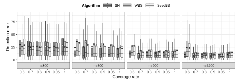
Figure 4.3: Detection error for SN, WBS and SeedBS algorithms across varying values of the coverage rate parameter, under the nonparametric model.

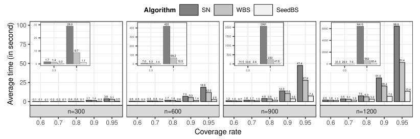
Figure 4.4: Computation time for SN, WBS and SeedBS algorithms across varying values of the coverage rate parameter, under the nonparametric model.

4.3 Comparison with the Two-step Method

We present a comparative analysis between the Reliever method and the two-step approach proposed by Kaul et al. (2019b). The two-step method is specifically designed to detect a single changepoint in a high-dimensional linear model. It involves an initial guess of the changepoint, which divides the data into two intervals. Proxy models are then fitted within these intervals. Consequently, both methods expedite the process of change detection by reducing extensive model fits. To mitigate the uncertainty in the initialization, multiple guesses are considered, and a changepoint estimator that minimizes the total loss on both segments is reported. In our study, we consider the high-dimensional linear model discussed in Section 5.1 of Kaul et al. (2019b), with $n=1200$ and $\tau^{\ast}=120$. We consider multiple initial guesses, specifically ${0.25n,0.5n,0.75n}$. The results presented in Table 4.1 indicate that although the two-step method may offer faster computation due to fewer model fits, it also exhibits larger detection errors. This can be attributed to its performance being heavily reliant on the accuracy of the initial changepoint estimate (or the quality of the corresponding intervals). In contrast, the Reliever method demonstrates stability across a range of choices for the parameter $r$, varying from $0.9$ to $0.3$.

Table 4.1: Comparison of detection error and average computational time between the Reliever method and the two-step method under the single changepoint setting with $(n,\delta_{m})=(1200,30)$. The numbers in parentheses represent the corresponding standard errors.

	Two-step	$r=0.9\,$	$r=0.7\,$	$r=0.5\,$	$r=0.3\,$
Error	$18.6(3.2)$	$9.2(1.0)$	$9.4(1.1)$	$7.6(0.8)$	$8.7(1.4)$
Time ($10$ms)	$60.7(0.6)$	$480.5(1.1)$	$141.0(0.4)$	$89.0(0.3)$	$64.1(0.3)$

The two-step method can be extended for multiple changepoint detection by incorporating the BS algorithm along with the multiple guess scheme, as suggested by Londschien et al. (2022). This extension can also be applied to the WBS and SeedBS methods in a similar manner. In our study, we examine the examples presented in Sections 4.1 and 4.2 with $n=1200$. Multiple initial guesses are selected as $m$-equally spaced quantiles within a search interval, following the recommendation by Londschien et al. (2022). The results depicted in Table 4.2 reveal that the two-step approach is less efficient for multiple changepoint detection, and increasing the number of multiple initial guesses can even have a detrimental impact on its performance. In contrast, the Reliever method (with $r=0.9$) exhibits performances that are almost comparable to the original implementation.

Table 4.2: Comparison of detection error and average computational time between the Reliever method and the two-step method under the multiple changepoint setting in Section 4.1 and 4.2. The numbers in parentheses represent the corresponding standard errors.

		$m=1\,$	$m=3\,$	$m=5\,$	Reliever	Original
High-dimensional	WBS	$19.7(0.9)$	$14.7(0.6)$	$16.8(0.8)$	$13.3(0.7)$	$12.1(0.6)$
	SeedBS	$21.4(1.0)$	$17.3(0.8)$	$17.8(0.8)$	$13.9(0.7)$	$12.0(0.6)$
Nonparametric	WBS	$85.5(3.2)$	$17.4(1.2)$	$17.5(1.2)$	$11.1(0.5)$	$13.6(1.0)$
	SeedBS	$87.5(3.2)$	$18.7(1.5)$	$17.6(1.2)$	$11.4(0.5)$	$14.1(1.0)$

5 Concluding Remarks

Searching for multiple changepoints in complex models with large datasets poses significant computational challenges. Current algorithms involve fitting a sequence of models and evaluating losses within numerous intervals during the search process. Existing approaches, such as PELT, WBS, SeedBS, and optimistic search algorithms, aim to reduce the number of (search) intervals. In this paper, we introduce Reliever which specifically relieves the computational burden by reducing the number of fitted models, as they are the primary contributors to computational costs. Our method associates each search interval with a deterministic (relief) interval from a pre-defined pool, enabling the fitting of models only within (or partially within) these selected intervals. The simplicity of the Reliever approach allows for seamless integration with various grid search algorithms and accommodates different models, providing tremendous potential for leveraging modern machine learning tools (Londschien et al., 2022; Liu et al., 2021; Li et al., 2022).

Reliever incorporates a coverage rate parameter, which balances computational efficiency and estimation accuracy. For high-dimensional regression models with changepoints, by employing an OP algorithm, we characterize requirements on the search path to ensure consistent and nearly rate-optimal estimators for changepoints; see Lemma 3.3. Our analysis demonstrates that the Reliever method satisfies these properties for any fixed coverage rate parameter. Further investigation is warranted to characterize the search path for other algorithms and broader model classes. Additionally, our theoretical analysis highlights the importance of adaptively selecting the nuisance parameter based on the underlying change magnitude. Future research should focus on extending the Reliever to enable data-driven selection of nuisance parameters. While the Reliever focuses on changepoint estimation, it is worth exploring the generalization of these concepts to quantify uncertainty in changepoint detection (Frick et al., 2014; Chen et al., 2023) and perform post-change-estimation inference (Jewell et al., 2022).

Appendix

Appendix A Conditions in Theorem 3.1

Define $\mathcal{L}(I,\bm{\theta})=\sum_{i\in I}\ell(\mathbf{z}_{i},\bm{\theta})$, $\overline{\mathcal{L}}(I,\bm{\theta})=\mathbb{E}\mathcal{L}(I,\bm{\theta})$, $G_{I}(\bm{\alpha})=|I|^{-1}\sum_{i\in I}g(\mathbf{z}_{i},\bm{\theta}_{I}^{\circ}+\bm{\alpha}|I|^{-1/2})$ and $\overline{G}_{I}(\bm{\alpha})=\mathbb{E}G_{I}(\bm{\alpha})$, where $g(\mathbf{z},\bm{\theta})=\nabla_{\bm{\theta}}\ell(\mathbf{z},\bm{\theta})$. The sub-Exponential norm of a sub-Exponential random variable $X$ is defined as $\lVert X\rVert_{\Psi_{1}}=\inf\{t>0:\mathbb{E}\exp(|X|/t)\leq 2\}$. For $\bm{X}\in\mathbb{R}^{p}$, we define $\lVert\mathbf{X}\rVert_{\Psi_{1}}=\sup_{\mathbf{v}\in\mathcal{S}^{p-1}}\lVert\mathbf{v}^{\top}\mathbf{X}\rVert_{\Psi_{1}}$.

1. $\ell(\cdot,\mathbf{z})$ is convex on the domain $\Theta$ for all fixed $\mathbf{z}$ and $\Theta$ is a compact and convex subset of $\mathbb{R}^{p}$.

2. The expectation $\mathbb{E}\ell(\mathbf{z}_{i},\bm{\theta})$ is finite for all $\mathbf{z}_{i}$ and fixed $\bm{\theta}\in\Theta$.

3. The population minimizer $\bm{\theta}_{I}^{\circ}$ uniquely exists and is interior point of $\Theta$.

4. $\lVert g(\mathbf{z}_{i},\bm{\theta})\rVert_{\Psi_{1}}\leq C_{\ref*{sec:proof_mest}.1}$ for each $\bm{\theta}$ near $\bm{\theta}_{I}^{\circ}$.

5. $\overline{\mathcal{L}}(I,\bm{\theta})$ is twice differentiable at $\bm{\theta}_{I}^{\circ}$ and $\mathbf{H}_{I}\triangleq|I|^{-1}\nabla_{\bm{\theta}}^{2}\overline{\mathcal{L}}(I,\bm{\theta}_{I}^{\circ})$ is positive-define.

6. $|\overline{G}_{I}(|I|^{\frac{1}{2}}(\bm{\theta}-\bm{\theta}_{I}^{\circ}))-\mathbf{H}_{I}(\bm{\theta}-\bm{\theta}_{I}^{\circ})|=C_{\ref*{sec:proof_mest}.2}\lVert{\bm{\theta}-\bm{\theta}_{I}^{\circ}}\rVert_{2}^{2}$.

7. $\lVert g(\mathbf{z}_{i},\bm{\theta})-g(\mathbf{z}_{i},\bm{\theta}_{I}^{\circ})\rVert_{\Psi_{1}}\leq C_{\ref*{sec:proof_mest}.3}\lVert\bm{\theta}-\bm{\theta}_{I}^{\circ}\rVert_{2}$.

1. $|I|^{-1}\overline{\mathcal{L}}(I,\bm{\theta})$ is $\rho$-strongly convex in the compact set $\Theta$.

2. $\mathbb{E}g(\mathbf{z}_{i},\bm{\theta})$ is $\zeta$-Lipschitz continuous w.r.t. $\bm{\theta}$.

3. For $i\in I\setminus R$, $\lVert\bm{\theta}_{R}^{\circ}-\bm{\theta}_{i}^{\circ}\rVert_{2}\leq\Delta_{\infty}$ where $\Delta_{\infty}>0$ is a fixed constant.

4. $\lVert\mathbf{H}_{R}^{-1}-\mathbf{H}_{I}^{-1}\rVert_{\mathsf{op}}\leq C_{\ref*{sec:proof_mest}.4}\lVert\bm{\theta}_{R}^{\circ}-\bm{\theta}_{I}^{\circ}\rVert_{2}$ and $\lVert\mathbf{H}_{I}^{-1}\rVert_{\mathsf{op}}\leq C_{\ref*{sec:proof_mest}.5}$ for any interval $I$.

Supplementary Material for “Reliever: Relieving the Burden of Costly Model Fits for Changepoint Detection”

Supplementary Material includes proofs of Theorem 3.1, Lemma 3.3 and Theorem 3.4, and additional simulation results.

Appendix A Proof of Theorem 3.1

For a fixed $\bm{\alpha}$, denote the random vectors $\mathbf{x}_{i}$ by

$$\mathbf{x}_{i}=g\Bigl{(}\mathbf{z}_{i},\bm{\theta}_{I}^{\circ}+\frac{\bm{\alpha}}{\sqrt{|I|}}\Bigr{)}-g(\mathbf{z}_{i},\bm{\theta}_{I}^{\circ}).$$

Denote $v_{I}=(\log n)^{1/2}$. By (g), uniformly for all $\lVert\bm{\alpha}\rVert_{2}\leq Mv_{I}$ (with some constant $M>0$), $\lVert\mathbf{x}_{i}\rVert_{\Psi_{1}}\leq C_{\ref*{sec:proof_mest}.3}Mv_{I}|I|^{-1/2}$. Therefore by applying an exponential inequality,

$$\sup_{\lVert\bm{\alpha}\rVert_{2}\leq Mv_{I}}\mathbb{P}\biggl{[}\Bigl{|}G_{I}(\bm{\alpha})-G_{I}(\bm{0})-\overline{G}_{I}(\bm{\alpha})\Bigr{|}\geq\frac{C_{u}C_{\ref*{sec:proof_mest}.3}M}{c_{b}}|I|^{-1}v_{I}\sqrt{\log n}\biggr{]}\leq 2\exp(-C_{u}\log n).$$

By (f),

$$\sup_{\lVert\bm{\alpha}\rVert_{2}\leq Mv_{I}}\Bigl{|}\frac{\mathbf{H}_{I}\bm{\alpha}}{\sqrt{|I|}}-\overline{G}_{I}(\bm{\alpha})\Bigr{|}\leq C_{\ref*{sec:proof_mest}.2}M^{2}v_{I}^{2}|I|^{-1}.$$

The above two inequalities imply that

$$\sup_{\lVert\bm{\alpha}\rVert_{2}\leq Mv_{I}}\mathbb{P}\biggl{[}\Bigl{|}G_{I}(\bm{\alpha})-G_{I}(\bm{0})-\frac{\mathbf{H}_{I}\bm{\alpha}}{\sqrt{|I|}}\Bigr{|}\geq\frac{C_{u}C_{\ref*{sec:proof_mest}.3}M}{c_{b}}|I|^{-1}v_{I}\sqrt{\log n}\biggr{]}\leq 2\exp(-C_{u}\log n).$$

By the chaining technique for convex function, i.e. the $\delta$-triangulation argument used in Niemiro (1992),

$$\mathbb{P}\biggl{[}\sup_{\lVert\bm{\alpha}\rVert_{2}\leq Mv_{I}}\Bigl{|}G_{I}(\bm{\alpha})-G_{I}(\bm{0})-\frac{\mathbf{H}_{I}\bm{\alpha}}{\sqrt{|I|}}\Bigr{|}\geq C_{\ref*{sec:proof_mest}.6}|I|^{-1}v_{I}\sqrt{\log n}\biggr{]}\leq 2|I|^{\frac{p}{2}}\exp(-C_{u}\log n).$$ (A.1)

By the sub-Exponential assumption, We can choose $M>0$ such that $\mathbb{P}[\lVert\sqrt{|I|}\mathbf{H}_{I}^{-1}G_{I}(\bm{0})\rVert_{2}\geq(M-1)\sqrt{\log n}]\leq 2\exp(-C_{u}\log n)$. It implies that with high probability, $\sqrt{|I|}\mathbf{H}_{I}^{-1}G_{I}(\bm{0})$ is in the ball $\{\mathbf{x}\in\mathbb{R}^{p}:\lVert\mathbf{x}\rVert_{2}<(M-1)\sqrt{\log n}\}$. For all $\mathbf{e}\in\mathbb{R}^{p}$ with $\lVert\mathbf{e}\rVert_{2}=1$, let $\bm{\alpha}=-\sqrt{|I|}\{\mathbf{H}_{I}^{-1}G_{I}(\bm{0})+(K\log n)|I|^{-1}\mathbf{e}\}$ with $K=2C_{\ref*{sec:proof_mest}.6}/\lambda_{\min}(\mathbf{H}_{I})$. With probability at least $1-2(1+|I|^{p/2})\exp(-C_{u}\log n)$,

$$\mathbf{e}^{\top}G_{I}\bigl{(}|I|^{\frac{1}{2}}\mathbf{H}_{I}^{-1}G_{I}(\bm{0})+(K\log n)|I|^{-1/2}\mathbf{e}\bigr{)}$$

$$\geq (K|I|^{-1}\log n)\cdot\mathbf{e}^{\top}\mathbf{H}_{I}\mathbf{e}-C_{\ref*{sec:proof_mest}.6}|I|^{-1}\log n>0.$$

It means that $\widehat{\bm{\theta}}_{I}$ is in the open ball $\{\bm{\theta}_{I}^{\circ}-\mathbf{H}_{I}^{-1}G_{I}(\bm{0})+(K\log n)|I|^{-1}\mathbf{e}:\lVert\mathbf{e}\rVert_{2}<1\}$. By taking the union bounds over the intervals $I\subset(0,n]$, uniformly with probability at least $1-\exp(-C_{\ref*{sec:proof_mest}.7}\log n)$,

$$(\widehat{\bm{\theta}}_{I}-\bm{\theta}_{I}^{\circ})=-\mathbf{H}_{I}^{-1}G_{I}(\bm{0})+\mathbf{r}_{I},$$ (A.2)

where $\max_{|I|\subset(0,n]}\mathbf{r}_{I}|I|/\log n=O(1)$.

Now we have obtained the uniform Bahadur representation that holds over $I\subset(0,n]$ with high probability. To measure the difference between $\widehat{\bm{\theta}}_{I}$ and $\widehat{\bm{\theta}}_{R}$, we first consider the population one. Recall that $R\in\mathcal{R}$ is the Relief interval of $I$. First of all, we study the population minimizers. By the $\rho$-strong convexity and the definition of $\bm{\theta}_{I}^{\circ}$ and $\bm{\theta}_{R}^{\circ}$,

$$0\leq\overline{\mathcal{L}}(I,\bm{\theta}_{R}^{\circ})-\overline{\mathcal{L}}(I,\bm{\theta}_{I}^{\circ})\leq\nabla_{\theta}\overline{\mathcal{L}}(I,\bm{\theta}_{R}^{\circ})^{\top}(\bm{\theta}_{R}^{\circ}-\bm{\theta}_{I}^{\circ})-\frac{\rho|I|}{2}\lVert\bm{\theta}_{R}^{\circ}-\bm{\theta}_{I}^{\circ}\rVert_{2}^{2},$$

which implies that

$$\lVert\bm{\theta}_{R}^{\circ}-\bm{\theta}_{I}^{\circ}\rVert_{2}\leq\frac{2}{\rho|I|}\Bigl{\lVert}\sum_{i\in I\setminus R}\mathbb{E}g(\mathbf{z}_{i},\bm{\theta}_{R}^{\circ})\Bigr{\rVert}_{2}\leq\frac{2\zeta}{\rho|I|}\sum_{i\in I\setminus R}\lVert\bm{\theta}_{R}^{\circ}-\bm{\theta}_{i}^{\circ}\rVert_{2}=O(1-r).$$

Assume that the Bahadur representation Eq. (A.2) holds thereinafter. We the following identity of the difference between $\widehat{\bm{\beta}}_{I}$ and $\widehat{\bm{\beta}}_{R}$,

$$\widehat{\bm{\theta}}_{I}-\widehat{\bm{\theta}}_{R}=\bm{\theta}_{I}^{\circ}-\bm{\theta}_{R}^{\circ}+\mathbf{H}_{R}^{-1}G_{R}(\bm{0})-\mathbf{H}_{I}G_{I}(\bm{0})+\mathbf{r}_{I}-\mathbf{r}_{R}.$$ (A.3)

For $\mathbf{H}_{R}^{-1}G_{R}(\bm{0})-\mathbf{H}_{I}G_{I}(\bm{0})$, further consider the following decomposition,

$$\mathbf{H}_{R}^{-1}G_{R}(\bm{0})-\mathbf{H}_{I}G_{I}(\bm{0})=(\mathbf{H}_{R}^{-1}-\mathbf{H}_{I}^{-1})G_{R}(\bm{0})+\mathbf{H}_{I}^{-1}\{G_{R}(\bm{0})-G_{I}(\bm{0})\}.$$

For the first part, by the sub-Exponential assumption (d), with probability at least $1-\exp(-C_{u}\log n)$,

$$\lVert(\mathbf{H}_{R}^{-1}-\mathbf{H}_{I}^{-1})G_{R}(\bm{0})\rVert_{2}\leq C_{\ref*{sec:proof_mest}.8}\lVert\bm{\theta}_{I}^{\circ}-\bm{\theta}_{R}^{\circ}\rVert_{2}\biggl{[}\Bigl{(}\frac{\log n}{|R|}\Bigr{)}^{\frac{1}{2}}+\frac{\log n}{|R|}\biggr{]}.$$ (A.4)

For the second part,

$$G_{R}(\bm{0})-G_{I}(\bm{0})=\sum_{i\in R}\Bigl{[}\frac{1}{|R|}g(\mathbf{z}_{i},\bm{\theta}_{R}^{\circ})-\frac{1}{|I|}g(\mathbf{z}_{i},\bm{\theta}_{I}^{\circ})\Bigr{]}-\sum_{i\in I\setminus R}\frac{1}{|I|}g(\mathbf{z}_{i},\bm{\theta}_{I}^{\circ})\triangleq\frac{1}{|I|}\sum_{i\in I}\mathbf{x}_{i},$$ (A.5)

where $\mathbf{x}_{i}=[g(\mathbf{z}_{i},\bm{\theta}_{R}^{\circ})|I|/|R|]-g(\mathbf{z}_{i},\bm{\theta}_{I}^{\circ})$ for $i\in R$ and $\mathbf{x}_{i}=-g(\mathbf{z}_{i},\bm{\theta}_{I}^{\circ})$ for $i\in I\setminus R$. For any individual $i\in R$, by assumptions (d) and (g),

$$\lVert\mathbf{x}_{i}\rVert_{\Psi_{1}} =\Bigl{\lVert}\{g(\mathbf{z}_{i},\bm{\theta}_{R}^{\circ})-g(\mathbf{z}_{i},\bm{\theta}_{I}^{\circ})\}+\frac{(1-r)}{r}g(\mathbf{z}_{i},\bm{\theta}_{R}^{\circ})\Bigr{\rVert}_{\Psi_{1}}$$

$$\leq\lVert\bm{\theta}_{I}^{\circ}-\bm{\theta}_{R}^{\circ}\rVert_{2}+\frac{1-r}{r}(C_{\ref*{sec:proof_mest}.3}\lVert\bm{\theta}_{R}^{\circ}-\bm{\theta}_{i}^{\circ}\rVert_{2}+C_{\ref*{sec:proof_mest}.1})\leq\lVert\bm{\theta}_{I}^{\circ}-\bm{\theta}_{R}^{\circ}\rVert_{2}+\frac{1-r}{r}C_{\ref*{sec:proof_mest}.9}$$

For $i\in I\setminus R$,

$$\lVert\mathbf{x}_{i}\rVert_{\Psi_{1}}\leq(C_{\ref*{sec:proof_mest}.3}\lVert\bm{\theta}_{I}^{\circ}-\bm{\theta}_{i}^{\circ}\rVert_{2}+C_{\ref*{sec:proof_mest}.1})\leq C_{\ref*{sec:proof_mest}.9}.$$

In the above two bounds, we use Condition (j), the boundness of parameters. By Bernstein’s inequality (Lemma C.1), with probability at least $1-\exp(-C_{u}\log n)$,

$$\lVert G_{R}(\bm{0})-G_{I}(\bm{0})\rVert_{2}=C_{\ref*{sec:proof_mest}.10}\biggl{[}\bigl{(}\lVert\bm{\theta}_{I}^{\circ}-\bm{\theta}_{R}^{\circ}\rVert_{2}+(1-r)^{\frac{1}{2}}\bigr{)}\Bigl{(}\frac{\log n}{|I|}\Bigr{)}^{\frac{1}{2}}+\frac{\log n}{|I|}\biggr{]}.$$ (A.6)

Overall we obtain,

$$\lVert\widehat{\bm{\theta}}_{I}-\widehat{\bm{\theta}}_{R}\rVert_{2}\leq O\biggl{(}\lVert\bm{\theta}_{I}^{\circ}-\bm{\theta}_{R}^{\circ}\rVert_{2}+(1-r)^{\frac{1}{2}}\Bigl{(}\frac{\log n}{|I|}\Bigr{)}^{\frac{1}{2}}+\frac{\log n}{|I|}\biggr{)}.$$ (A.7)

By the definition of $\widehat{\bm{\theta}}_{R}$, one obtains $\nabla_{\bm{\theta}}\mathcal{L}(I,\widehat{\bm{\theta}}_{R})=\sum_{i\in I\setminus R}g(\mathbf{z}_{i},\widehat{\bm{\theta}}_{R})$. Similarly, by the $\delta$-triangulation argument used in the proof of the Bahadur representation, with probability at least $1-\exp(-C_{u}\log n)$, uniformly for all intervals $I$,

$$\Bigl{\lVert}\sum_{i\in I\setminus R}\Bigl{\{}g(\mathbf{z}_{i},\widehat{\bm{\theta}}_{R})-g(\mathbf{z}_{i},\bm{\theta}_{R}^{\circ})-\mathbb{E}\bigl{[}g(\mathbf{z}_{i},\widehat{\bm{\theta}}_{R})-g(\mathbf{z}_{i},\bm{\theta}_{R}^{\circ})\bigr{]}\Bigr{\}}\Bigr{\rVert}_{2}=O(\log n),$$

$$\Bigl{\lVert}\sum_{i\in I\setminus R}\mathbb{E}\{g(\mathbf{z}_{i},\widehat{\bm{\theta}}_{R})-g(\mathbf{z}_{i},\bm{\theta}_{R}^{\circ})\}\Bigr{\rVert}_{2}\leq\zeta(1-r)\lVert\widehat{\bm{\theta}}_{R}-\bm{\theta}_{R}^{\circ}\rVert_{2}=O((1-r)\sqrt{|I|\log n}+\log n),$$

$$\Bigl{\lVert}\sum_{i\in I\setminus R}g(\mathbf{z}_{i},\bm{\theta}_{R}^{\circ})\Bigr{\rVert}_{2}=\Bigl{\lVert}\sum_{i\in I\setminus R}\mathbb{E}g(\mathbf{z}_{i},\bm{\theta}_{R}^{\circ})\Bigr{\rVert}_{2}+O(\sqrt{(1-r)|I|\log n}+\log n).$$

Combining the above three upper bounds,

$$\nabla_{\bm{\theta}}\mathcal{L}(I,\widehat{\bm{\theta}}_{R})=\Bigl{\lVert}\sum_{i\in I\setminus R}\mathbb{E}g(\mathbf{z}_{i},\bm{\theta}_{R}^{\circ})\Bigr{\rVert}_{2}+O\bigl{(}(1-r)\sqrt{|I|\log n}+\log n\bigr{)}.$$ (A.8)

By the convexity condition (h),

$$\frac{1}{|I|}\{\mathcal{L}(I,\widehat{\bm{\theta}}_{R})-\mathcal{L}(I,\widehat{\bm{\theta}}_{I})\}\leq\frac{1}{|I|}\nabla_{\bm{\theta}}\mathcal{L}(I,\widehat{\bm{\theta}}_{R})^{\top}(\widehat{\bm{\theta}}_{R}-\widehat{\bm{\theta}}_{I})\leq\frac{1}{|I|}\lVert\nabla_{\bm{\theta}}\mathcal{L}(I,\widehat{\bm{\theta}}_{R})\rVert_{2}\lVert\widehat{\bm{\theta}}_{R}-\widehat{\bm{\theta}}_{I}\rVert_{2}$$

$$= O\biggl{(}\frac{1}{\rho|I|^{2}}\Bigl{\lVert}\sum_{i\in I\setminus R}\mathbb{E}g(\mathbf{z}_{i},\bm{\theta}_{R}^{\circ})\Bigr{\rVert}_{2}^{2}+(1-r)\frac{\log n}{|I|}+\frac{(\log n)^{2}}{|I|^{2}}\biggr{)}.$$ (A.9)

When $I=(s,e]$ contains no changepoint, or it is nearly homogeneous such that if a true changepoint $\tau\in I$, then $\min(\tau-s,e-\tau)=O(\log n)$, we have $\sum_{i\in I\setminus R}\mathbb{E}g(\mathbf{z}_{i},\bm{\theta}_{R}^{\circ})=O(\min(\tau-s,e-\tau))=O(\log n)$. Therefore,

$$\frac{1}{|I|}\{\mathcal{L}(I,\widehat{\bm{\theta}}_{R})-\mathcal{L}(I,\widehat{\bm{\theta}}_{I})\}=O\biggl{(}(1-r)\frac{\log n}{|I|}+\frac{(\log n)^{2}}{|I|^{2}}\biggr{)}.$$ (A.10)

Appendix B Proof of Lemma 3.3

We first introduce some notations. For a given changepoint estimation $\tau\in[n]$ and a changepoints set $\mathcal{T}=\{0<\tau_{1}<\dots<\tau_{K}<\tau_{K+1}<n\}$, denote $\mathcal{K}_{+}(\tau,\mathcal{T})\triangleq\min_{k}\{k:\tau_{k}>\tau\}$ and $\mathcal{K}_{-}(\tau,\mathcal{T})\triangleq\max_{k}\{k:\tau_{k}<\tau\}$. For simplicity, further denote $k_{\tau,+}^{\ast}=\mathcal{K}_{+}(\tau,\mathcal{T}^{\ast})$, $\widehat{k}_{\tau,+}=\mathcal{K}_{+}(\tau,\widehat{\mathcal{T}})$, $k_{\tau,-}^{\ast}=\mathcal{K}_{-}(\tau,\mathcal{T}^{\ast})$ and $\widehat{k}_{\tau,-}=\mathcal{K}_{-}(\tau,\widehat{\mathcal{T}})$. Let $\widehat{\mathcal{T}}=\{\widehat{\tau}_{1},\dots,\widehat{\tau}_{\widehat{K}}\}$ be the minimizer of Eq. (3.7). Denote $\delta_{m}=C_{m}s\log(p\vee n)$ and $\delta_{k}=2\widetilde{C}s\log(p\vee n)\Delta_{k}^{-2}$ where $\Delta_{k}=\lVert\bm{\beta}_{k+1}^{\ast}-\bm{\beta}_{k}^{\ast}\rVert_{\Sigma}$, and $\mathcal{H}=\{(\widehat{\tau}_{a},\widehat{\tau}_{a+1}]:\exists h\in[K^{\ast}],\min(\tau_{h}^{\ast}-\widehat{\tau}_{a},\widehat{\tau}_{a+1}-\tau_{h}^{\ast})>\delta_{h}\}$.

Assume that $\mathcal{H}\neq\emptyset$, i.e. $\exists h\in[K^{\ast}]$ such that $\widehat{\mathcal{T}}\cap[\tau_{h}^{\ast}-\delta_{h},\tau_{h}^{\ast}+\delta_{h}]=\emptyset$. For such $h$ and $a$, without loss of generality assume that $\tau_{h}^{\ast}-\widehat{\tau}_{a}>\delta_{h}$, it can be observed that $(\tau_{h}^{\ast}-\delta_{h},\tau_{h}^{\ast}+\delta_{h}]\subset(\widehat{\tau}_{a},\widehat{\tau}_{a+1}]$ and $\Delta_{(\widehat{\tau}_{a},\widehat{\tau}_{a+1}]}^{2}(\widehat{\tau}_{a+1}-\widehat{\tau}_{a})\geq 2\delta_{h}\Delta_{(\tau_{h}^{\ast}-\delta_{h},\tau_{h}^{\ast}+\delta_{h}]}^{2}=\frac{\delta_{h}\Delta_{h}^{2}}{2}=\widetilde{C}s\log(p\vee n)$.

To move further, we need the following definitions to divide $\mathcal{H}$ into four groups.

Definition B.1 (Separability of a point).

For a changepoint estimation $\tau$ and the true changepoint set $\mathcal{T}^{\ast}$, let $u=k_{\tau,-}^{\ast}$ and $v=k_{\tau,+}^{\ast}$. We say that $\tau$ is separable from the left if $\tau-\tau_{u}^{\ast}>\delta_{u}\vee\delta_{m}$ and separable from the right if $\tau_{v}^{\ast}-\tau>\delta_{v}\vee\delta_{m}$. Otherwise, $\tau$ is inseparable from the left (right).

Definition B.2 (Separability of an interval).

For the intervals $(\tau_{l},\tau_{r}]\in\mathcal{H}$, we make the following definitions,

1. $(\tau_{l},\tau_{r}]\in(0,n]$ is separable if $\tau_{l}$ is separable from the right and $\tau_{r}$ is separable from the left.

2. $(\tau_{l},\tau_{r}]\in(0,n]$ is left-separable if $\tau_{l}$ is separable from the right and $\tau_{r}$ is inseparable from the left.

3. $(\tau_{l},\tau_{r}]\in(0,n]$ is right-separable if $\tau_{l}$ is inseparable from the right and $\tau_{r}$ is separable from the left.

4. $(\tau_{l},\tau_{r}]\in(0,n]$ is inseparable if $\tau_{l}$ is inseparable from the right and $\tau_{r}$ is inseparable from the left.

Now the sub-intervals in $\mathcal{H}$ have been classified into four groups $\mathcal{H}=\mathcal{H}_{1}\cup\mathcal{H}_{2}\cup\mathcal{H}_{3}\cup\mathcal{H}_{4}$. We will show that $\mathcal{H}=\emptyset$ by emptying these groups.

Case 1: $\mathcal{H}_{1}=\emptyset$

For $(\widehat{\tau}_{a},\widehat{\tau}_{a+1}]\in\mathcal{H}_{1}$, let $h=k_{\widehat{\tau}_{a},+}^{\ast}$. Denote $\mathcal{T}_{a}=\{\tau_{h}^{\ast},\dots,\tau_{h+t}^{\ast}\}=\mathcal{T}^{\ast}\cap(\widehat{\tau}_{a},\widehat{\tau}_{a+1})$. Let $\widetilde{\mathcal{T}}=\widehat{\mathcal{T}}\cup\mathcal{T}_{a}$. Since $\gamma=C_{\gamma}s\log(p\vee n)$,

$$L(\widehat{\mathcal{T}})-L(\widetilde{\mathcal{T}})=C_{(\widehat{\tau}_{a},\widehat{\tau}_{a+1}]}-\Bigl{[}C_{(\widehat{\tau}_{a},\tau_{h}^{\ast}]}+C_{(\tau_{h+t}^{\ast},\widehat{\tau}_{a+1}]}+\sum_{j=h}^{h+t-1}C_{(\tau_{j}^{\ast},\tau_{j+1}^{\ast}]}+(t+1)\gamma\Bigr{]}$$

$$> (1-C_{\ref*{lem:loc_err_g}.3})\Delta_{(\widehat{\tau}_{a},\widehat{\tau}_{a+1}]}^{2}(\widehat{\tau}_{a+1}-\widehat{\tau}_{a})-(t+2)C_{\ref*{lem:loc_err_g}.1}s\log(p\vee n)-(t+1)\gamma$$

$$= (1-C_{\ref*{lem:loc_err_g}.3})\sum_{i\in(\widehat{\tau}_{a},\widehat{\tau}_{a+1}]}\lVert\bm{\beta}_{i}^{\circ}-\bm{\beta}_{(\widehat{\tau}_{a},\widehat{\tau}_{a+1}]}^{\circ}\rVert_{\Sigma}^{2}-[(t+2)C_{\ref*{lem:loc_err_g}.1}+(t+1)C_{\gamma}]s\log(p\vee n)$$

$$\geq \Bigl{[}(1-C_{\ref*{lem:loc_err_g}.3})(t+1)\tilde{C}-(t+2)C_{\ref*{lem:loc_err_g}.1}-(t+1)C_{\gamma}\Bigr{]}s\log(p\vee n)>0,$$

provided that $\tilde{C}\geq(1-C_{\ref*{lem:loc_err_g}.3})^{-1}(2C_{\ref*{lem:loc_err_g}.1}+C_{\gamma})$. Therefore $\mathcal{H}_{1}=\emptyset$.

Case 2: $\mathcal{H}_{2}=\mathcal{H}_{3}=\emptyset$

Without loss of generality, by the symmetry of $\mathcal{H}_{2}$ and $\mathcal{H}_{3}$, we only show that $\mathcal{H}_{3}=\emptyset$. If the claim does not hold, one can choose $(\widehat{\tau}_{a},\widehat{\tau}_{a+1}]\in\mathcal{H}_{3}$ to be the leftmost one. Hence $\widehat{\tau}_{a}$ must be separable from the left by Condition 3.1. Since $\mathcal{H}_{1}=\emptyset$ and $(\widehat{\tau}_{a},\widehat{\tau}_{a+1}]$ is the leftmost interval in $\mathcal{H}_{3}$, one obtains $(\widehat{\tau}_{a-1},\widehat{\tau}_{a}]\not\in\mathcal{H}$. Denote $h=k_{\widehat{\tau}_{a},+}^{\ast}$ and $\mathcal{T}_{a}=\mathcal{T}^{\ast}\cap(\widehat{\tau}_{a}+\delta_{m},\widehat{\tau}_{a+1}-\delta_{m})=\{\tau_{h+1}^{\ast},\dots,\tau_{h+t}^{\ast}\}$ ($t=0$ if $\mathcal{T}_{a}=\emptyset$). Let $\widetilde{\mathcal{T}}=(\widehat{\mathcal{T}}\setminus{\widehat{\tau}_{a}})\cup{\tau_{h}^{\ast}}\cup\mathcal{T}_{a}=(\widehat{\mathcal{T}}\setminus{\widehat{\tau}_{a}})\cup\{\tau_{j}^{\ast}\}_{j=h}^{h+t}$.

$$L(\widehat{\mathcal{T}})-L(\widetilde{\mathcal{T}})= C_{(\widehat{\tau}_{a},\widehat{\tau}_{a+1}]}+\bigl{(}C_{(\widehat{\tau}_{a-1},\widehat{\tau}_{a}]}-C_{(\widehat{\tau}_{a-1},\tau_{h}^{\ast}]}\bigr{)}-\Bigl{[}\sum_{j=h}^{h+t-1}C_{(\tau_{j}^{\ast},\tau_{j+1}^{\ast}]}+C_{(\tau_{h+t}^{\ast},\widehat{\tau}_{a+1}]}+t\gamma\Bigr{]}$$

$$> (1-C_{\ref*{lem:loc_err_g}.3})\Delta_{(\widehat{\tau}_{a},\widehat{\tau}_{a+1}]}^{2}(\widehat{\tau}_{a+1}-\widehat{\tau}_{a})-[(t+1)C_{\ref*{lem:loc_err_g}.1}+tC_{\gamma}]s\log(p\vee n)$$

$$+ \Bigl{(}\sum_{i\in(\widehat{\tau}_{a},\tau_{h}^{\ast}]}\epsilon_{i}^{2}+C_{(\widehat{\tau}_{a-1},\widehat{\tau}_{a}]}-C_{(\widehat{\tau}_{a-1},\tau_{h}^{\ast}]}\Bigr{)}.$$ (B.1)

Since $(\widehat{\tau}_{a-1},\widehat{\tau}_{a}]\not\in\mathcal{H}$ and $0<\widehat{\tau}_{a}-\tau_{h}^{\ast}<\delta_{m}$, one must obtain that either $(\widehat{\tau}_{a-1},\widehat{\tau}_{a})\cap\mathcal{T}^{\ast}=\emptyset$ or $0<\tau_{h-1}^{\ast}-\widehat{\tau}_{a-1}<\delta_{h-1}=2\widetilde{C}\Delta_{h-1}^{-2}s\log(p\vee n)$.

For the first scenario, under $\mathbb{G}_{1}$,

$$\Bigl{|}\sum_{i\in(\widehat{\tau}_{a},\tau_{h}^{\ast}]}\epsilon_{i}^{2}+C_{(\widehat{\tau}_{a-1},\widehat{\tau}_{a}]}-C_{(\widehat{\tau}_{a-1},\tau_{h}^{\ast}]}\Bigr{|}\leq 2C_{\ref*{lem:loc_err_g}.1}s\log(p\vee n).$$ (B.2)

Hence,

$$L(\widehat{\mathcal{T}})-L(\widetilde{\mathcal{T}}) >(1-C_{\ref*{lem:loc_err_g}.3})\Delta_{(\widehat{\tau}_{a},\widehat{\tau}_{a+1}]}^{2}(\widehat{\tau}_{a+1}-\widehat{\tau}_{a})-[(t+3)C_{\ref*{lem:loc_err_g}.1}+tC_{\gamma}]s\log(p\vee n)$$

$$\geq\Bigl{\{}(1-C_{\ref*{lem:loc_err_g}.3})(t\vee 1)\tilde{C}-(t+3)C_{\ref*{lem:loc_err_g}.1}-tC_{\gamma}\Bigr{\}}s\log(p\vee n)>0,$$

provided that $\tilde{C}\geq(1-C_{\ref*{lem:loc_err_g}.3})^{-1}(4C_{\ref*{lem:loc_err_g}.1}+C_{\gamma})$.

For the second scenario, let $I_{1}=(\widehat{\tau}_{a-1},\widehat{\tau}_{a}]$ and $I_{2}=(\widehat{\tau}_{a-1},\tau_{h}^{\ast}]$. Firstly, we will bound the gap $\Delta_{I_{2}}^{2}|I_{2}|-\Delta_{I_{1}}^{2}|I_{1}|$. Since $I_{1}\subset I_{2}$, we have $\Delta_{I_{2}}^{2}|I_{2}|-\Delta_{I_{1}}^{2}|I_{1}|\geq 0$.

Denote $d_{1}=\tau_{h-1}^{\ast}-\widehat{\tau}_{a-1}$, $d_{2}=\widehat{\tau}_{a}-\tau_{h-1}^{\ast}$ and $d_{3}=\tau_{h}^{\ast}-\widehat{\tau}_{a}$. Recall that $\Delta_{h-1}=\lVert\bm{\beta}_{h}^{\ast}-\bm{\beta}_{h-1}^{\ast}\rVert_{\Sigma}$ and the definition of $\Delta_{I}^{2}$, we have

$$\Delta_{I_{2}}^{2}|I_{2}|=\frac{d_{1}(d_{2}+d_{3})}{d_{1}+d_{2}+d_{3}}\Delta_{h-1}^{2},\,\Delta_{I_{1}}^{2}|I_{1}|=\frac{d_{1}d_{2}}{d_{1}+d_{2}}\Delta_{h-1}^{2}.$$

It follows that

$$\Delta_{I_{2}}^{2}|I_{2}|-\Delta_{I_{1}}^{2}|I_{1}|=\frac{d_{1}^{2}d_{3}\Delta_{h-1}^{2}}{(d_{1}+d_{2})(d_{1}+d_{2}+d_{3})}\leq\frac{\widetilde{C}^{2}(\widetilde{C}\vee C_{m})}{C_{\mathsf{snr}}(C_{\mathsf{snr}}-\widetilde{C}\vee C_{m})}s\log(p\vee n).$$

where the last inequality is from the conditions $d_{1}\leq\widetilde{C}\Delta_{h-1}^{-2}s\log(p\vee n)$, $d_{3}\leq\delta_{h}\vee\delta_{m}$ and $d_{1}+d_{2}+d_{3}\geq C_{\mathsf{snr}}s\log(p\vee n)[1+\Delta_{h-1}^{-2}+\Delta_{h}^{-2}]$. Denote $C_{m,1}=\frac{\widetilde{C}^{2}(\widetilde{C}\vee C_{m})}{C_{\mathsf{snr}}(C_{\mathsf{snr}}-\widetilde{C}\vee C_{m})}$.

By $0<\tau_{h-1}^{\ast}-\widehat{\tau}_{a-1}<\delta_{h-1}=2\widetilde{C}\Delta_{h-1}^{-2}s\log(p\vee n)$, $\Delta_{I_{1}}^{2}|I_{1}|\leq\Delta_{I_{2}}^{2}|I_{2}|\leq\widetilde{C}s\log(p\vee n)$. Hence combining $\mathbb{G}_{2}$,

$$\sum_{i\in(\widehat{\tau}_{a},\tau_{h}^{\ast}]}\epsilon_{i}^{2}+C_{(\widehat{\tau}_{a-1},\widehat{\tau}_{a}]}-C_{(\widehat{\tau}_{a-1},\tau_{h}^{\ast}]}>-(2C_{\ref*{lem:loc_err_g}.2}+C_{m,1})s\log(p\vee n).$$ (B.3)

By Eq. (B) and Eq. (B.3),

$$L(\widehat{\mathcal{T}})-L(\widetilde{\mathcal{T}}) >(1-C_{\ref*{lem:loc_err_g}.3})\Delta_{(\widehat{\tau}_{a},\widehat{\tau}_{a+1}]}^{2}(\widehat{\tau}_{a+1}-\widehat{\tau}_{a})-[(t+1)C_{\ref*{lem:loc_err_g}.1}+tC_{\gamma}+2C_{\ref*{lem:loc_err_g}.2}+C_{m,1}]s\log(p\vee n)$$

$$\geq[(1-C_{\ref*{lem:loc_err_g}.3})(t\vee 1)\tilde{C}-(t+1)C_{\ref*{lem:loc_err_g}.1}-tC_{\gamma}-2C_{\ref*{lem:loc_err_g}.2}-C_{m,1}]s\log(p\vee n)>0,$$

provided that $\tilde{C}\geq(1-C_{\ref*{lem:loc_err_g}.3})^{-1}(2C_{\ref*{lem:loc_err_g}.1}+C_{\gamma}+2C_{\ref*{lem:loc_err_g}.2}+C_{m,1})$. Hence $\mathcal{H}_{2}\cup\mathcal{H}_{3}=\emptyset$.

Case 3: $\mathcal{H}_{4}=\emptyset$

Similar to Case 2, let $(\widehat{\tau}_{a},\widehat{\tau}_{a+1}]\in\mathcal{H}_{4}$, then $\widehat{\tau}_{a}$ is separable from the left and $\widehat{\tau}_{a+1}$ is separable from the right. By the fact that $\mathcal{H}_{1}\cup\mathcal{H}_{2}\cup\mathcal{H}_{3}=\emptyset$, we also obtain $(\widehat{\tau}_{a-1},\widehat{\tau}_{a}]\not\in\mathcal{H}$ and $(\widehat{\tau}_{a+1},\widehat{\tau}_{a+2}]\not\in\mathcal{H}$. Let $h=k_{\widehat{\tau}_{a},+}^{\ast}$ and $h+t=k_{\widehat{\tau}_{a+1},-}^{\ast}$. Denote $\mathcal{T}_{a}=\{\tau_{h}^{\ast},\dots,\tau_{h+t}^{\ast}\}$ and $\widetilde{\mathcal{T}}=(\widehat{\mathcal{T}}\setminus\{\widehat{\tau}_{a},\widehat{\tau}_{a+1}\}\cup\mathcal{T}_{a}$. We have

$$L(\widehat{\mathcal{T}})-L(\widetilde{\mathcal{T}})= C_{(\widehat{\tau}_{a},\widehat{\tau}_{a+1}]}+[C_{(\widehat{\tau}_{a-1},\widehat{\tau}_{a}]}+C_{(\widehat{\tau}_{a+1},\widehat{\tau}_{a+2}]}-C_{(\widehat{\tau}_{a-1},\tau_{h}^{\ast}]}-C_{(\tau_{h+t}^{\ast},\widehat{\tau}_{a+2}]}]$$

$$- \sum_{j=h}^{h+t-1}C_{(\tau_{j}^{\ast},\tau_{j+1}^{\ast}]}-(t-1)\gamma$$

$$> (1-C_{\ref*{lem:loc_err_g}.3})\Delta_{(\widehat{\tau}_{a},\widehat{\tau}_{a+1}]}^{2}(\widehat{\tau}_{a+1}-\widehat{\tau}_{a})-(tC_{\ref*{lem:loc_err_g}.1}+(t-1)C_{\gamma})s\log(p\vee n)$$

$$+ [\sum_{i\in(\widehat{\tau}_{a},\tau_{h}^{\ast}]\cup(\tau_{h+1}^{\ast},\widehat{\tau}_{a+1}]}\epsilon_{i}^{2}+C_{(\widehat{\tau}_{a-1},\widehat{\tau}_{a}]}+C_{(\widehat{\tau}_{a+1},\widehat{\tau}_{a+2}]}-C_{(\widehat{\tau}_{a-1},\tau_{h}^{\ast}]}-C_{(\tau_{h+t}^{\ast},\widehat{\tau}_{a+2}]}].$$

Follow the same discussion in Case 2, see Eq. (B.3), we have

$$\sum_{i\in(\widehat{\tau}_{a},\tau_{h}^{\ast}]\cup(\tau_{h+1}^{\ast},\widehat{\tau}_{a+1}]}\epsilon_{i}^{2}+C_{(\widehat{\tau}_{a-1},\widehat{\tau}_{a}]}+C_{(\widehat{\tau}_{a+1},\widehat{\tau}_{a+2}]}-C_{(\widehat{\tau}_{a-1},\tau_{h}^{\ast}]}-C_{(\tau_{h+t}^{\ast},\widehat{\tau}_{a+2}]}>-(4C_{\ref*{lem:loc_err_g}.2}+2C_{m,1})s\log(p\vee n).$$ (B.4)

Hence,

$$L(\widehat{\mathcal{T}})-L(\widetilde{\mathcal{T}})$$

$$> (1-C_{\ref*{lem:loc_err_g}.3})\Delta_{(\widehat{\tau}_{a},\widehat{\tau}_{a+1}]}^{2}(\widehat{\tau}_{a+1}-\widehat{\tau}_{a})-[tC_{\ref*{lem:loc_err_g}.1}+(t-1)C_{\gamma}+4C_{\ref*{lem:loc_err_g}.2}+2C_{m,1}]s\log(p\vee n)$$

$$\geq \Bigl{\{}(1-C_{\ref*{lem:loc_err_g}.3})[(t-1)\vee 1]\tilde{C}-tC_{\ref*{lem:loc_err_g}.1}-(t-1)C_{\gamma}-4C_{\ref*{lem:loc_err_g}.2}-2C_{m,1}\Bigr{\}}s\log(p\vee n)\geq 0$$

provided that $\tilde{C}\geq(1-C_{\ref*{lem:loc_err_g}.3})^{-1}(2C_{\ref*{lem:loc_err_g}.1}+C_{\gamma}+4C_{\ref*{lem:loc_err_g}.2}+2C_{m,1})$.

In summary, we obtain $\mathcal{H}=\emptyset$ provided that $\tilde{C}\geq(1-C_{\ref*{lem:loc_err_g}.3})^{-1}(2C_{\ref*{lem:loc_err_g}.1}+C_{\gamma}+4C_{\ref*{lem:loc_err_g}.2}+2C_{m,1})$. Hence $\max_{1\leq j\leq K^{\ast}}\min_{1\leq k\leq\widehat{K}}\frac{1}{2}\Delta_{j}^{2}|\tau_{j}^{\ast}-\widehat{\tau}_{k}|\leq\tilde{C}s\log(p\vee n)$. It also implies that $\widehat{K}\geq K^{\ast}$.

It remains to show that $\widehat{K}\leq K^{\ast}$. Otherwise, assume that $\widehat{K}>K^{\ast}$. Then there must be $j\in[0,K^{\ast}]$ and $k\in[1,\widehat{K}]$ such that $\tau_{j}^{\ast}-\delta_{j}\leq\widehat{\tau}_{k-1}<\widehat{\tau}_{k}<\widehat{\tau}_{k+1}\leq\tau_{j+1}^{\ast}+\delta_{j+1}$. Similar to the decomposition of $\mathcal{H}$, we can also divide it into four groups.

1. $\tau_{j}^{\ast}\leq\widehat{\tau}_{k-1}<\widehat{\tau}_{k}<\widehat{\tau}_{k+1}\leq\tau_{j+1}^{\ast}$.

2. $\tau_{j}^{\ast}-\delta_{j}\leq\widehat{\tau}_{k-1}<\tau_{j}^{\ast}$ and $\tau_{j}^{\ast}\leq\widehat{\tau}_{k}<\widehat{\tau}_{k+1}\leq\tau_{j+1}^{\ast}$.

3. $\tau_{j}^{\ast}\leq\widehat{\tau}_{k-1}<\widehat{\tau}_{k}\leq\tau_{j+1}^{\ast}$ and $\tau_{j+1}^{\ast}<\widehat{\tau}_{k+1}\leq\tau_{j+1}^{\ast}+\delta_{j+1}$.

4. $\tau_{j}^{\ast}-\delta_{j}\leq\widehat{\tau}_{k-1}<\tau_{j}^{\ast}\leq\widehat{\tau}_{k}\leq\tau_{j+1}^{\ast}<\widehat{\tau}_{k+1}\leq\tau_{j+1}^{\ast}+\delta_{j+1}$

Case 1: $\mathcal{G}_{1}=\emptyset$

Let $\widetilde{\mathcal{T}}=\widehat{\mathcal{T}}\setminus\{\widehat{\tau}_{k}\}$. We have

$$L(\widetilde{\mathcal{T}})-L(\widehat{\mathcal{T}}) =C_{(\widehat{\tau}_{k-1},\widehat{\tau}_{k+1}]}-C_{(\widehat{\tau}_{k-1},\widehat{\tau}_{k}]}-C_{(\widehat{\tau}_{k},\widehat{\tau}_{k+1}]}-\gamma$$

$$<(3C_{\ref*{lem:loc_err_g}.1}-C_{\gamma})s\log(p\vee n)\leq 0,$$

provided that $C_{\gamma}\geq 3C_{\ref*{lem:loc_err_g}.1}$.

Case 2: $\mathcal{G}_{2}\cup\mathcal{G}_{3}=\emptyset$

We will show that $\mathcal{G}_{2}=\emptyset$ because the proof for $\mathcal{G}_{3}=\emptyset$ is the same by symmetry. Assume that $j$ and $k$ are the leftmost one that satisfies $\mathcal{G}_{2}$. It implies that $\widehat{\tau}_{k-2}\in[\tau_{j-1}^{\ast}-\delta_{j-1},\tau_{j-1}^{\ast}+\delta_{j-1}]$. Otherwise assume $\widehat{\tau}_{k-2}>\tau_{j-1}^{\ast}+\delta_{j-1}$. Since $\max_{1\leq j\leq K^{\ast}}\min_{1\leq k\leq\widehat{K}}\Delta_{j}^{2}|\tau_{j}^{\ast}-\widehat{\tau}_{k}|\leq\widetilde{C}s\log(p\vee n)$, there must be $\widehat{\tau}_{k-h}\in[\tau_{j-1}^{\ast}-\delta_{j-1},\tau_{j-1}^{\ast}+\delta_{j-1}]$ for some $h>2$. It contradicts the fact that $\mathcal{G}_{1}=\emptyset$ and the choice of $k$.

Let $\widetilde{\mathcal{T}}=\{\tau_{j}^{\ast}\}\cup\widehat{\mathcal{T}}\setminus\{\widehat{\tau}_{k-1},\widehat{\tau}_{k}\}$.

$$L(\widetilde{\mathcal{T}})-L(\widehat{\mathcal{T}}) =C_{(\widehat{\tau}_{k-2},\tau_{j}^{\ast}]}+C_{(\tau_{j}^{\ast},\widehat{\tau}_{k+1}]}-\Bigl{[}\sum_{t=k-2}^{k}C_{(\widehat{\tau}_{t},\widehat{\tau}_{t+1}]}+\gamma\Bigr{]}$$

$$=[C_{(\widehat{\tau}_{k-2},\tau_{j}^{\ast}]}-C_{(\widehat{\tau}_{k-2},\widehat{\tau}_{k-1}]}]+C_{(\tau_{j}^{\ast},\widehat{\tau}_{k+1}]}-\Bigl{[}\sum_{t=k-1}^{k}C_{(\widehat{\tau}_{t},\widehat{\tau}_{t+1}]}+\gamma\Bigr{]}$$

$$<\Bigl{[}C_{(\widehat{\tau}_{k-2},\tau_{j}^{\ast}]}-C_{(\widehat{\tau}_{k-2},\widehat{\tau}_{k-1}]}-\sum_{i\in(\widehat{\tau}_{k-1},\tau_{j}^{\ast}]}\epsilon_{i}^{2}\Bigr{]}+(2C_{\ref*{lem:loc_err_g}.1}+C_{\ref*{lem:loc_err_g}.2}-C_{\gamma})s\log(p\vee n)$$

$$\leq(2C_{\ref*{lem:loc_err_g}.1}+3C_{\ref*{lem:loc_err_g}.2}+C_{m,1}-C_{\gamma})s\log(p\vee n)\leq 0,$$

provided $C_{\gamma}\geq 2C_{\ref*{lem:loc_err_g}.1}+3C_{\ref*{lem:loc_err_g}.2}+C_{m,1}$. The second last inequality is from Eq. (B.3).

Case 3: $\mathcal{G}_{4}=\emptyset$

Now $\mathcal{G}_{1}\cup\mathcal{G}_{2}\cup\mathcal{G}_{3}=\emptyset$. Assume that $\{\widehat{\tau}_{k-1},\widehat{\tau}_{k},\widehat{\tau}_{k+1}\}$ satisfies $\mathcal{G}_{4}$. Similar to the analysis of $\mathcal{G}_{2}=\emptyset$, we have $\widehat{\tau}_{k-2}\in[\tau_{j-1}^{\ast}-\delta_{j-1},\tau_{j-1}^{\ast}+\delta_{j-1}]$ and $\widehat{\tau}_{k+2}\in[\tau_{j+1}^{\ast}+\delta_{j+1},\tau_{j+1}^{\ast}+\delta_{j+1}]$. Follow the same arguments in the proof for $\mathcal{H}_{4}=\emptyset$, we can set $\widetilde{\mathcal{T}}=\{\tau_{j}^{\ast},\tau_{j+1}^{\ast}\}\cup\widehat{\mathcal{T}}\setminus\{\widehat{\tau}_{k-1},\widehat{\tau}_{k},\widehat{\tau}_{k+1}\}$.

$$L(\widetilde{\mathcal{T}})-L(\widehat{\mathcal{T}}) =C_{(\widehat{\tau}_{k-2},\tau_{j}^{\ast}]}+C_{(\tau_{j}^{\ast},\tau_{j+1}^{\ast}]}+C_{(\tau_{j+1}^{\ast},\widehat{\tau}_{k+2}]}-\Bigl{[}\sum_{t=k-2}^{k+1}C_{(\widehat{\tau}_{t},\widehat{\tau}_{t+1}]}+\gamma\Bigr{]}$$

$$=[C_{(\widehat{\tau}_{k-2},\tau_{j}^{\ast}]}-C_{(\widehat{\tau}_{k-2},\widehat{\tau}_{k-1}]}+C_{(\tau_{j+1}^{\ast},\widehat{\tau}_{k+2}]}-C_{(\widehat{\tau}_{k+1},\widehat{\tau}_{k+2}]}]$$

$$+C_{(\tau_{j}^{\ast},\tau_{j+1}^{\ast}]}-\Bigl{[}\sum_{t=k-1}^{k}C_{(\widehat{\tau}_{t},\widehat{\tau}_{t+1}]}+\gamma\Bigr{]}$$

$$<\Bigl{[}C_{(\widehat{\tau}_{k-2},\tau_{j}^{\ast}]}-C_{(\widehat{\tau}_{k-2},\widehat{\tau}_{k-1}]}+C_{(\tau_{j+1}^{\ast},\widehat{\tau}_{k+2}]}-C_{(\widehat{\tau}_{k+1},\widehat{\tau}_{k+2}]}-\sum_{i\in(\widehat{\tau}_{k-1},\tau_{j}^{\ast}]\cup(\tau_{j+1}^{\ast},\widehat{\tau}_{k+1}]}\epsilon_{i}^{2}\Bigr{]}$$

$$+(C_{\ref*{lem:loc_err_g}.1}+2C_{\ref*{lem:loc_err_g}.2}-C_{\gamma})s\log(p\vee n)$$

$$\leq(C_{\ref*{lem:loc_err_g}.1}+6C_{\ref*{lem:loc_err_g}.2}+2C_{m,1}-C_{\gamma})s\log(p\vee n)\leq 0,$$

provided $C_{\gamma}\geq C_{\ref*{lem:loc_err_g}.1}+6C_{\ref*{lem:loc_err_g}.2}+2C_{m,1}$. The second last inequality is from Eq. (B.3).

Combining the proof in the $\mathcal{H}$ and $\mathcal{G}$ parts, we can determine the two constants by solving the following inequalities,

$$\left\{\begin{aligned} C_{\gamma}&\geq C_{\ref*{lem:loc_err_g}.1}+6C_{\ref*{lem:loc_err_g}.2}+2C_{m,1}\\ \widetilde{C}&\geq(1-C_{\ref*{lem:loc_err_g}.3})^{-1}(2C_{\ref*{lem:loc_err_g}.1}+C_{\gamma}+4C_{\ref*{lem:loc_err_g}.2}+2C_{m,1})\end{aligned}\right.$$ (B.5)

Since $C_{\mathsf{snr}}$ and $C_{m}$ are sufficiently large, $C_{m,1}=\frac{\widetilde{C}^{2}(\widetilde{C}\vee C_{m})}{C_{\mathsf{snr}}(C_{\mathsf{snr}}-\widetilde{C}\vee C_{m})}=\frac{\widetilde{C}^{2}C_{m}}{C_{\mathsf{snr}}(C_{\mathsf{snr}}-C_{m})}$. Let $C_{\gamma}=C_{\ref*{lem:loc_err_g}.1}+6C_{\ref*{lem:loc_err_g}.2}+2C_{m,1}$, one obtains the following inequality w.r.t. $\widetilde{C}$,

$$\frac{4C_{m}\widetilde{C}^{2}}{C_{\mathsf{snr}}(C_{\mathsf{snr}}-C_{m})}-(1-C_{\ref*{lem:loc_err_g}.3})\widetilde{C}+3C_{\ref*{lem:loc_err_g}.1}+10C_{\ref*{lem:loc_err_g}.2}\geq 0.$$

Treat it as a quadratic inequality w.r.t. $\widetilde{C}$, we can figure out that there exist solutions if and only if $C_{\mathsf{snr}}(C_{\mathsf{snr}}-C_{m})\geq 16(1-C_{\ref*{lem:loc_err_g}.3})^{-2}C_{m}(3C_{\ref*{lem:loc_err_g}.1}+10C_{\ref*{lem:loc_err_g}.2})$. And by solving it, we have

$$\widetilde{C}=a-\sqrt{a^{2}-b}\leq\frac{b}{2\sqrt{a^{2}-b}}\leq\frac{b}{a}=2(1-C_{\ref*{lem:loc_err_g}.3})^{-1}(3C_{\ref*{lem:loc_err_g}.1}+10C_{\ref*{lem:loc_err_g}.2}),$$ (B.6)

satisfies Eq. (B.5). Here $a=\frac{(1-C_{\ref*{lem:loc_err_g}.3})C_{\mathsf{snr}}(C_{\mathsf{snr}}-C_{m})}{8C_{m}}$ and $b=\frac{(3C_{\ref*{lem:loc_err_g}.1}+10C_{\ref*{lem:loc_err_g}.2})C_{\mathsf{snr}}(C_{\mathsf{snr}}-C_{m})}{4C_{m}}$. The last inequality in Eq. (B.6) holds provided that $C_{\mathsf{snr}}$ is sufficiently large such that $b\leq 3a^{2}/4$.

And it follows that $\widehat{\mathcal{T}}=\widetilde{\mathcal{T}}$ provided that Eq. (B.5) holds. Finally, we obtain

$$\widehat{K}=K^{\ast};\max_{1\leq k\leq K^{\ast}}\min_{1\leq j\leq\widehat{K}}\frac{1}{2}\Delta_{k}^{2}|\tau_{k}^{\ast}-\widehat{\tau}_{j}|\leq\widetilde{C}s\log(p\vee n),$$ (B.7)

with $\widetilde{C}=2(1-C_{\ref*{lem:loc_err_g}.3})^{-1}(3C_{\ref*{lem:loc_err_g}.1}+10C_{\ref*{lem:loc_err_g}.2})$.

Appendix C Proof of Theorem 3.4

For a interval $I$, denote the sparsity constant $s_{I}=s\vee|\{1\leq j\leq p:\exists i\in I,\bm{\beta}_{i,j}^{\circ}\neq 0\}|\geq s$. Observe that $s_{I}\leq|\mathcal{T}^{\ast}\cap I|\times s$. Define $\Delta_{I,q}=({|I|}^{-1}\sum_{i\in I}\lVert\bm{\beta}_{i}^{\circ}-\bm{\beta}_{I}^{\circ}\rVert_{\Sigma}^{q})^{{1}/{q}}$ and $\Delta_{I}=\Delta_{I,2}$ be the root average square variation of $I$ and $\Delta_{I,\infty}=\max_{i\in I}\lVert\bm{\beta}_{i}^{\circ}-\bm{\beta}_{I}^{\circ}\rVert_{\Sigma}$ be the maximum variation of $I$. As stated in Lemma 3.3, to show that the bound of localization error in Theorem 3.4 holds, we only need to certify that the event $\mathbb{G}$ holds with high probability for both the original full model-fitting approach and the Reliever approach with suitable constants. These two claims are shown in Corollary C.8 and Corollary C.11, respectively. Finally, the $L_{2}$ error bound of the parameter estimation follows the oracle inequality of LASSO.

This section is organized as follows. In Section C.1, we introduce several useful non-asymptotic probability bounds, including the oracle inequality of LASSO with heterogeneous data. In Section C.2 and C.3, we show that $\mathbb{G}$ holds with high probability for the two approaches correspondingly. All the proofs are relegated to the last part.

C.1 Supporting Lemmas

Lemma C.1 (Bernstein’s inequality; Proposition 2.8.1. in vershynin_high-dimensional_2018).

Let $X_{1},\dots,X_{n}$ be independent, mean zero, sub-exponential random variables. For every $t>0$, we have

$$\mathbb{P}\Bigl{\{}\Bigl{|}\sum_{i=1}^{n}X_{i}\Bigr{|}>t\Bigr{\}}\leq 2\exp\Bigl{[}-c_{b}\Bigl{(}\frac{t^{2}}{\sum_{i=1}^{n}\lVert X_{i}\rVert_{\Psi_{1}}^{2}}\wedge\frac{t}{\max_{i}\lVert X_{i}\rVert_{\Psi_{1}}}\Bigr{)}\Bigr{]},$$

where $c_{b}>0$ is an absolute constant. Choose $t=\frac{C_{u}}{c_{b}}[\sqrt{\sum_{i\in[n]}\lVert X_{i}\rVert_{\Psi_{1}}^{2}\log(p\vee n)}\vee\{\max_{i}\lVert X_{i}\rVert_{\Psi_{1}}\log(p\vee n)\}]$ with $C_{u}\geq c_{b}$, we have

$$\mathbb{P}\Bigl{\{}\Bigl{|}\sum_{i=1}^{n}X_{i}\Bigr{|}>t\Bigr{\}}\leq 2\exp\{-C_{u}\log(p\vee n)\},$$

Lemma C.2 (Uniform Restricted Eigenvalue Condition).

Assume Condition 3.3 (a) holds. For any interval $I\subset(0,n]$, denote $\widehat{\Sigma}_{I}=|I|^{-1}\sum_{i\in I}\mathbf{x}_{i}\mathbf{x}_{i}^{\top}$. Uniformly for all intervals $I\subset(0,n]$ such that $|I|\geq s_{I}\log(p\vee n)$, with probability at least $1-\exp\{-C_{u,1}\log(p\vee n)\}$,

$$\mathbf{v}^{\top}\widehat{\Sigma}_{I}\mathbf{v}\geq\lVert\mathbf{v}\rVert_{\Sigma}^{2}-C_{u,2}C_{x}^{2}\sigma_{x}^{2}\sqrt{\frac{s_{I}\log(p\vee n)}{|I|}}(\lVert\mathbf{v}\rVert_{2}^{2}+\frac{1}{s_{I}}\lVert\mathbf{v}\rVert_{1}^{2}),\,\forall\mathbf{v}\in\mathbb{R}^{p},$$

where $C_{u,1}$ and $C_{u,2}$ are two universal constants. Let $|I|\geq C_{\mathsf{re}}s_{I}\log(p\vee n)$ with a sufficiently large constant $C_{\mathsf{re}}\geq 1\vee(\frac{34C_{u,2}C_{x}^{2}\sigma_{x}^{2}}{\underline{\kappa}})^{2}$. For any support set $\mathcal{S}\in[p]$ with $|\mathcal{S}|\leq s_{I}$ and $\mathbf{v}\in\mathbb{R}^{p}$ such that $\lVert\mathbf{v}_{\mathcal{S}^{\complement}}\rVert_{1}\leq 3\lVert\mathbf{v}_{\mathcal{S}}\rVert_{1}$, under the same event above,

$$\mathbf{v}^{\top}\widehat{\Sigma}_{I}\mathbf{v}\geq\frac{\underline{\kappa}}{2}\lVert\mathbf{v}\rVert_{2}^{2}.$$

Lemma C.3.

Assume Condition 3.3 holds. With probability at least $1-\exp\{-C_{u,1}\log(p\vee n)\}$, uniformly for any sub-interval $I\subset(0,n]$,

$$\Bigl{\lVert}\sum_{i\in I}\mathbf{x}_{i}[\mathbf{x}_{i}^{\top}(\bm{\beta}_{i}^{\circ}-\bm{\beta}_{I}^{\circ})+\epsilon_{i}]\Bigr{\rVert}_{\infty}$$

$$\leq C_{u,2}C_{x}\sigma_{x}\sqrt{(C_{x}^{2}\Delta_{I}^{2}+C_{\epsilon}^{2})\vee\frac{(C_{x}^{2}\Delta_{I,\infty}^{2}+C_{\epsilon}^{2})\log(p\vee n)}{|I|}}\sqrt{|I|\log(p\vee n)}$$

$$\leq C_{u,2}C_{x}\sigma_{x}\sqrt{(C_{x}^{2}\Delta_{I}^{2}+C_{\epsilon}^{2})\vee\frac{(C_{x}^{2}\sigma_{x}^{2}C_{\beta}^{2}s_{I}+C_{\epsilon}^{2})\log(p\vee n)}{|I|}}\sqrt{|I|\log(p\vee n)},$$

where $C_{u,2}=c_{b}^{-1}(C_{u,1}+3)$, $\Delta_{I}^{2}=\frac{1}{|I|}\sum_{i\in I}\lVert\bm{\beta}_{i}^{\circ}-\bm{\beta}_{I}^{\circ}\rVert_{\Sigma}^{2}$ is the mean square variation and $\Delta_{I,\infty}=\max_{i\in I}\lVert\bm{\beta}_{i}^{\circ}-\bm{\beta}_{I}^{\circ}\rVert_{\Sigma}$ is the maximum jumps.

Lemma C.4.

Denote $\Delta_{I,4}=(\frac{1}{|I|}\sum_{i\in I}\lVert\bm{\beta}_{i}^{\circ}-\bm{\beta}_{I}^{\circ}\rVert_{\Sigma}^{4})^{\frac{1}{4}}$. Assume Condition 3.3 holds. With probability at least $1-\exp\{-C_{u,1}\log(p\vee n)\}$, uniformly for any sub-interval $I\subset(0,n]$,

$$\Bigl{|}\sum_{i\in I}\{\mathbf{x}_{i}^{\top}(\bm{\beta}_{i}^{\circ}-\bm{\beta}_{I}^{\circ})\}^{2}-\Delta_{I}^{2}|I|\Bigr{|}\leq C_{u,2}C_{x}^{2}\sqrt{\Delta_{I,4}^{4}\vee\frac{\Delta_{I,\infty}^{4}\log(p\vee n)}{|I|}}\sqrt{|I|\log(p\vee n)}$$

$$\leq C_{u,2}C_{x}^{2}\sqrt{\Delta_{I}^{2}\vee\frac{C_{\beta}^{2}\sigma_{x}^{2}s_{I}\log(p\vee n)}{|I|}}\sqrt{C_{\beta}^{2}\sigma_{x}^{2}|I|s_{I}\log(p\vee n)}.$$

Lemma C.5.

Assume Condition 3.3 holds. With probability at least $1-\exp\{-C_{u,1}\log(p\vee n)\}$, uniformly for any sub-interval $I\subset(0,n]$,

$$\Bigl{|}\sum_{i\in I}\mathbf{x}_{i}^{\top}(\bm{\beta}_{i}^{\circ}-\bm{\beta}_{I}^{\circ})\epsilon_{i}\Bigr{|}\leq C_{u,2}C_{x}C_{\epsilon}\sqrt{\Delta_{I}^{2}\vee\frac{\Delta_{I,\infty}^{2}\log(p\vee n)}{|I|}}\sqrt{|I|\log(p\vee n)},$$

Lemma C.6 (Oracle inequalities).

Assume Condition 3.2 (a) and Condition 3.3 hold. For any interval $I\subset(0,n]$, let $D_{I}=\sqrt{(C_{x}^{2}\Delta_{I}^{2}+C_{\epsilon}^{2})\vee\frac{(C_{x}^{2}\Delta_{I,\infty}^{2}+C_{\epsilon}^{2})\log(p\vee n)}{|I|}}$. We have with probability at least $1-2\exp\{-C_{u,1}\log(p\vee n)\}$, uniformly for any interval $I\subset(0,n]$ with $|I|\geq C_{\mathsf{re}}s_{I}\log(p\vee n)$, provided that $\lambda_{I}=4C_{u,2}C_{x}\sigma_{x}D_{I}\sqrt{|I|\log(p\vee n)}$, the solution $\widehat{\bm{\beta}}_{I}$ satisfies that

$$\lVert\widehat{\bm{\beta}}_{I}-\bm{\beta}_{I}^{\circ}\rVert_{2}\leq C_{\ref*{lem:oracle}}D_{I}\sqrt{\frac{s_{I}\log(p\vee n)}{|I|}},$$

$$\lVert\widehat{\bm{\beta}}_{I}-\bm{\beta}_{I}^{\circ}\rVert_{1}\leq C_{\ref*{lem:oracle}}D_{I}s_{I}\sqrt{\frac{\log(p\vee n)}{|I|}},$$

where the model-based constant $C_{\ref*{lem:oracle}}=\frac{12C_{u,2}C_{x}\sigma_{x}}{\underline{\kappa}}$.

C.2 Certifying $\mathbb{G}$ for the Full Model-fitting

Lemma C.7 (in-sample error).

Assume Condition 3.2 and Condition 3.3 (a) hold. For any interval $I\subset(0,n]$, let $D_{I}=\sqrt{(C_{x}^{2}\Delta_{I}^{2}+C_{\epsilon}^{2})\vee\frac{(C_{x}^{2}\Delta_{I,\infty}^{2}+C_{\epsilon}^{2})\log(p\vee n)}{|I|}}$. Under the setting in Lemma C.6, with probability at least $1-4\exp\{-C_{u,1}\log(p\vee n)\}$, for any interval $I=(\tau_{l},\tau_{r}]$ such that $|I|\geq C_{\mathsf{re}}s_{I}\log(p\vee n)$,

$$\Bigl{|}\mathcal{L}_{I}-\sum_{i\in I}\epsilon_{i}^{2}-\Delta_{I}^{2}|I|\Bigr{|}\leq\frac{48C_{u,2}^{2}C_{x}^{2}\sigma_{x}^{2}D_{I}^{2}s_{I}\log(p\vee n)}{\underline{\kappa}}$$

$$+ C_{u,2}C_{x}(C_{x}\Delta_{I,\infty}+2C_{\epsilon})\sqrt{[(\Delta_{I}^{2}|I|)\vee\{\Delta_{I,\infty}^{2}\log(p\vee n)\}]\log(p\vee n)}.$$

Additionally if Condition 3.3 (b) holds,

$$\Bigl{|}\mathcal{L}_{I}-\sum_{i\in I}\epsilon_{i}^{2}-\Delta_{I}^{2}|I|\Bigr{|}\leq\frac{48C_{u,2}^{2}C_{x}^{2}\sigma_{x}^{2}D_{I}^{2}s_{I}\log(p\vee n)}{\underline{\kappa}}$$

$$+ C_{u,2}C_{x}(C_{x}\sigma_{x}C_{\beta}+\frac{2C_{\epsilon}}{\sqrt{s_{I}}})\sqrt{[(\Delta_{I}^{2}|I|)\vee\{\sigma_{x}^{2}C_{\beta}^{2}s_{I}\log(p\vee n)\}]s_{I}\log(p\vee n)}.$$

Corollary C.8.

Assume Condition 3.1, Condition 3.2, and Condition 3.3 hold. Under the same probability event in Lemma C.7 and with sufficiently large $C_{m}$, we have the following conclusions.

1. For $I$ such that $\Delta_{I}=0$ and $|I|\geq C_{m}s\log(p\vee n)$,

   $$\Bigl{|}\mathcal{L}_{I}-\sum_{i\in I}\epsilon_{i}^{2}\Bigr{|}\leq\frac{48C_{u,2}^{2}C_{x}^{2}\sigma_{x}^{2}C_{\epsilon}^{2}s\log(p\vee n)}{\underline{\kappa}}\triangleq C_{\ref*{cor:in_err}.1}s\log(p\vee n).$$

2. For $I$ such that $\Delta_{I}^{2}|I|\leq\widetilde{C}s\log(p\vee n)$ for some sufficiently large $\widetilde{C}\geq 2C_{\beta}^{2}\sigma_{x}^{2}$, $|I\cap\mathcal{T}^{\ast}|\leq 1$ and $|I|\geq C_{m}s\log(p\vee n)$,

   $$\Bigl{|}\mathcal{L}_{I}-\sum_{i\in I}\epsilon_{i}^{2}-\Delta_{I}^{2}|I|\Bigr{|}\leq C_{\ref*{cor:in_err}.2}s\log(p\vee n),$$

   where $C_{\ref*{cor:in_err}.2}=2C_{\ref*{cor:in_err}.1}+\frac{96C_{u,2}^{2}C_{x}^{4}\sigma_{x}^{2}\widetilde{C}}{C_{m}\underline{\kappa}}+C_{u,2}C_{x}(C_{x}\sigma_{x}C_{\beta}+\frac{2C_{\epsilon}}{\sqrt{s}})\sqrt{2\widetilde{C}}$.

3. For $I$ such that $|I|\geq C_{m}s\log(p\vee n)$ and $\Delta_{I}^{2}|I|\geq\widetilde{C}s\log(p\vee n)$ for some sufficiently large $\widetilde{C}\geq 3C_{\beta}^{2}\sigma_{x}^{2}$,

   $$\mathcal{L}_{I}-\sum_{i\in I}\epsilon_{i}^{2}\geq(1-C_{\ref*{cor:in_err}.3})\Delta_{I}^{2}|I|,$$

   where

   $$C_{\ref*{cor:in_err}.3}=\frac{96C_{u,2}^{2}C_{x}^{4}\sigma_{x}^{2}}{\underline{\kappa}C_{m}}+C_{u,2}C_{x}\biggl{(}C_{x}\sigma_{x}C_{\beta}+\frac{2C_{\epsilon}}{\sqrt{s}}\biggr{)}\sqrt{\frac{3}{\widetilde{C}}}+\frac{3C_{\ref*{cor:in_err}.1}}{\widetilde{C}}.$$

C.3 Certifying $\mathbb{G}$ for Reliever

Notations: Let $R$ be the surrogate interval w.r.t. $I$ and $J=I\setminus R$ be the complement. Denote $\overline{\Delta}_{I}^{2}=\frac{1}{|I|}\sum_{i\in I}\lVert\bm{\beta}_{i}^{\circ}-\bm{\beta}_{R}^{\circ}\rVert_{\Sigma}^{2}$, $\widetilde{\Delta}_{J}^{2}=\frac{1}{|J|}\sum_{i\in J}\lVert\bm{\beta}_{i}^{\circ}-\bm{\beta}_{R}^{\circ}\rVert_{\Sigma}^{2}$ and $\widehat{\Delta}_{J}^{2}=\frac{1}{|J|}\sum_{i\in J}\lVert\bm{\beta}_{i}^{\circ}-\widehat{\bm{\beta}}_{R}\rVert_{\Sigma}^{2}$. Let $\widetilde{\Delta}_{J,q}^{q}=\frac{1}{|J|}\sum_{i\in J}\lVert\bm{\beta}_{i}^{\circ}-\bm{\beta}_{R}^{\circ}\rVert_{\Sigma}^{q}$. The following identity holds for these variations, $\overline{\Delta}_{I}^{2}|I|=\Delta_{R}^{2}|R|+\widetilde{\Delta}_{J}^{2}|J|$. Denote the cost function of interval $I$ by $\overline{\mathcal{L}}_{I}=\sum_{i\in I}(y_{i}-\mathbf{x}_{i}^{\top}\widehat{\bm{\beta}}_{R})^{2}$.

Lemma C.9 (mixed-sample error).

Assume Condition 3.2 and Condition 3.3 (a) hold. With probability at least $1-4\exp\{-C_{u,1}\log(p\vee n)\}$, for any interval $I=(\tau_{l},\tau_{r}]$ such that $|R|\geq C_{\mathsf{re}}s_{R}\log(p\vee n)$,

$$\Bigl{|}\overline{\mathcal{L}}_{I}-\sum_{i\in I}\epsilon_{i}^{2}-\widehat{\Delta}_{J}^{2}|J|-\Delta_{R}^{2}|R|\Bigr{|}\leq\frac{48C_{u,2}^{2}C_{x}^{2}\sigma_{x}^{2}D_{R}^{2}s_{R}\log(p\vee n)}{\underline{\kappa}}$$

$$+ C_{u,2}C_{x}(C_{x}\Delta_{R,\infty}+2C_{\epsilon})\sqrt{[(\Delta_{R}^{2}|R|)\vee\{\Delta_{R,\infty}^{2}\log(p\vee n)\}]\log(p\vee n)}$$

$$+ C_{u,2}C_{x}(C_{x}\widehat{\Delta}_{J,\infty}+2C_{\epsilon})\sqrt{[(\widehat{\Delta}_{J}^{2}|J|)\vee\{\widehat{\Delta}_{J,\infty}^{2}\log(p\vee n)\}]\log(p\vee n)}$$

In the final bound of Lemma C.9, there exists a random variation term $\widehat{\Delta}_{J}^{2}$. To obtain deterministic result, we will show that $|\widehat{\Delta}_{J}^{2}-\widetilde{\Delta}_{J}^{2}||J|$ is relatively small in the following lemma.

Lemma C.10 (bound for the random variation).

Assume Condition 3.2 and Condition 3.3 hold. Assume that the joint probability event of Lemmas C.2–C.4 holds, which implies a probability lower bound $1-3\exp\{-C_{u,1}\log(p\vee n)\}$. For any $I=(\tau_{l},\tau_{r}]\in(0,n]$ such that $|I|\geq C_{m}s\log(p\vee n)$ and $|R|\geq r|I|$, the set $J=I\setminus R$ satisfies that,

• For $I$ such that $\Delta_{I}=0$ and $|I|\geq C_{m}s\log(p\vee n)$,

  $$\bigl{|}\widehat{\Delta}_{J}^{2}-\widetilde{\Delta}_{J}^{2}\bigr{|}|J|\leq C_{\ref*{lem:oracle}}^{2}\sigma_{x}^{2}\frac{|J|}{|R|}C_{\epsilon}^{2}s\log(p\vee n)\leq\frac{C_{\ref*{lem:oracle}}^{2}C_{\epsilon}^{2}\sigma_{x}^{2}(1-r)}{r}s\log(p\vee n).$$

  Also since $|R|\geq rC_{m}s\log(p\vee n)$, we have the upper bound for the average term,

  $$\widehat{\Delta}_{J,\infty}^{2}=\widehat{\Delta}_{J}^{2}=\Bigl{|}\widehat{\Delta}_{J}^{2}-\widetilde{\Delta}_{J}^{2}\Bigr{|}\leq\frac{C_{\ref*{lem:oracle}}^{2}\sigma_{x}^{2}C_{\epsilon}^{2}}{|R|}s\log(p\vee n)\leq\frac{C_{\ref*{lem:oracle}}^{2}\sigma_{x}^{2}C_{\epsilon}^{2}}{C_{m}r}.$$

• For $I$ such that $\Delta_{I}^{2}|I|\leq\widetilde{C}s\log(p\vee n)$, $|I\cap\mathcal{T}^{\ast}|\leq 1$ and $|I|\geq C_{m}s\log(p\vee n)$, we have

  $$\bigl{|}\widehat{\Delta}_{J}^{2}-\widetilde{\Delta}_{J}^{2}\bigr{|}|J|\leq C_{\ref*{lem:rd_var}.1}s\log(p\vee n),$$

  where

  $$C_{\ref*{lem:rd_var}.1}=4C_{\ref*{lem:oracle}}\sigma_{x}\sqrt{\frac{1-r}{r}}\sqrt{\frac{2C_{x}^{2}\widetilde{C}^{2}}{C_{m}r}+C_{\epsilon}\widetilde{C}}+2C_{\ref*{lem:oracle}}^{2}\sigma_{x}^{2}\frac{1-r}{r}\Bigl{(}\frac{2C_{x}^{2}\widetilde{C}}{C_{m}r}+C_{\epsilon}^{2}\Bigr{)}.$$

• For $I$ such that $|I|\geq C_{m}s\log(p\vee n)$ and $\Delta_{I}^{2}|I|\geq\widetilde{C}s\log(p\vee n)$,

  $$\bigl{|}\widehat{\Delta}_{J}^{2}-\widetilde{\Delta}_{J}^{2}\bigr{|}|J|\leq C_{\ref*{lem:rd_var}.2}\overline{\Delta}_{I}^{2}|I|,$$

  where

  $$C_{\ref*{lem:rd_var}.2}=2C_{\ref*{lem:oracle}}\sigma_{x}\sqrt{\frac{1-r}{r}}\sqrt{\frac{2C_{x}^{2}}{C_{m}r}+\frac{3C_{\epsilon}^{2}}{\widetilde{C}}}+C_{\ref*{lem:oracle}}^{2}\sigma_{x}^{2}\frac{1-r}{r}\Bigl{(}\frac{2C_{x}^{2}}{C_{m}r}+\frac{3C_{\epsilon}^{2}}{\widetilde{C}}\Bigr{)}.$$

Remark.

Both of the constants $C_{\ref*{lem:rd_var}.1}$ and $C_{\ref*{lem:rd_var}.2}$ are $o(1)$ provided that $|J|=o(|R|)$.

Corollary C.11.

Assume Condition 3.2 and Condition 3.3 hold. Here we only consider those intervals $I$ such that $|I|\geq C_{m}s\log(p\vee n)$ for some sufficiently large constant $C_{m}$. With probability at least $1-4\exp\{-C_{u,1}\log(p\vee n)\}$, we have the following conclusions uniformly.

1. If $\Delta_{I}=0$,

   $$\Bigl{|}\overline{\mathcal{L}}_{I}-\sum_{i\in I}\epsilon_{i}^{2}\Bigr{|}\leq C_{\ref*{cor:mix_err}.1}s\log(p\vee n),$$

   where $C_{\ref*{cor:mix_err}.1}=C_{\ref*{cor:in_err}.1}+\frac{(1-r)C_{\ref*{lem:oracle}}^{2}\sigma_{x}^{2}C_{\epsilon}^{2}}{r}+C_{u,2}C_{x}(\frac{C_{x}C_{\ref*{lem:oracle}}^{2}\sigma_{x}^{2}C_{\epsilon}^{2}}{\sqrt{C_{m}r}}+2C_{\epsilon}^{2}C_{\ref*{lem:oracle}}\sigma_{x})\sqrt{\frac{(1-r)}{rs}\vee\frac{1}{C_{m}rs^{2}}}$.

2. For $I$ such that $\Delta_{I}^{2}|I|\leq\widetilde{C}s\log(p\vee n)$ for some sufficiently large $\widetilde{C}\geq 3C_{\beta}^{2}\sigma_{x}^{2}$, $|I\cap\mathcal{T}^{\ast}|\leq 1$ and $|I|\geq C_{m}s\log(p\vee n)$, we have

   $$\Bigl{|}\overline{\mathcal{L}}_{I}-\sum_{i\in I}\epsilon_{i}^{2}-\overline{\Delta}_{I}^{2}|I|\Bigr{|}\leq C_{\ref*{cor:mix_err}.2}s\log(p\vee n),$$

   where $C_{\ref*{cor:mix_err}.2}=2C_{\ref*{cor:in_err}.1}+C_{\ref*{lem:rd_var}.1}+\frac{96C_{u,2}^{2}C_{x}^{4}\sigma_{x}^{2}\widetilde{C}}{C_{m}r\underline{\kappa}}+C_{u,2}C_{x}(\sqrt{3}C_{x}\sigma_{x}C_{\beta}+\frac{2C_{\epsilon}}{\sqrt{s}})[\widetilde{C}^{\frac{1}{2}}+(2\widetilde{C}+C_{\ref*{lem:rd_var}.1})^{\frac{1}{2}}]$.

3. If $\Delta_{I}^{2}|I|\geq\widetilde{C}s\log(p\vee n)$ for some sufficiently large $\widetilde{C}\geq 3C_{\beta}^{2}\sigma_{x}^{2}$,

   $$\overline{\mathcal{L}}_{I}-\sum_{i\in I}\epsilon_{i}^{2}\geq(1-C_{\ref*{cor:mix_err}.3})\overline{\Delta}_{I}^{2}|I|,$$

   where $C_{\ref*{cor:mix_err}.3}=C_{\ref*{lem:rd_var}.2}+\frac{3C_{\ref*{cor:in_err}.1}}{\widetilde{C}}+\frac{96C_{u,2}^{2}C_{x}^{4}\sigma_{x}^{2}}{C_{m}r\underline{\kappa}}+\frac{C_{u,2}C_{x}\sqrt{3}}{\sqrt{\widetilde{C}}}(C_{x}\sigma_{x}C_{\beta}+\frac{2C_{\epsilon}}{\sqrt{s}})(1+\sqrt{1+C_{\ref*{lem:rd_var}.2}})$.

C.4 Proofs

Proof of Lemma C.2.

To ease the notation, we will replace $s_{I}$ with $s$ without loss of generality in the proof. Denote $\mathcal{A}(s)=\{\mathbf{v}\in\mathbb{R}^{p}:\lVert\mathbf{v}\rVert_{2}=1,|\operatorname*{\mathrm{supp}}(\mathbf{v})|\leq s\}$. We will show that with high probability, $\sup_{\mathbf{v}\in\mathcal{A}(2s)}|\mathbf{v}^{\top}(\widehat{\Sigma}_{I}-\Sigma)\mathbf{v}|=O(C_{x}^{2}\sqrt{\frac{s\log(p\vee n)}{|I|}})$, then the result follows from Lemma 12 in loh_high-dimensional_2012. Let $\mathbf{D}=\widehat{\Sigma}_{I}-\Sigma$.

For any $\mathcal{U}\subset[p]$ and $|\mathcal{U}|=2s$, let $\mathbf{D}_{\mathcal{U}}\in\mathbb{R}^{s\times s}$ be the sub-matrix of $\mathbf{D}$ with $\mathcal{U}$ being the set of row and column indices. Let $\mathcal{B}_{\mathcal{U}}=\{\mathbf{v}\in\mathbb{R}^{p}:\lVert\mathbf{v}\rVert_{2}=1,\operatorname*{\mathrm{supp}}(\mathbf{v})=\mathcal{U}\}$. There is a $\frac{1}{4}$-net $\mathcal{N}_{\mathcal{U}}$ of $\mathcal{B}_{\mathcal{U}}$ with cardinality $|\mathcal{N}_{\mathcal{U}}|\leq 9^{s}$. For any $\mathbf{v}\in\mathcal{B}_{\mathcal{U}}-\mathcal{N}_{\mathcal{U}}$, there is $\mathbf{u}\in\mathcal{N}_{\mathcal{U}}$ such that $\lVert\mathbf{v}-\mathbf{u}\rVert_{2}\leq\frac{1}{4}$ and $\frac{\mathbf{v}-\mathbf{u}}{\lVert\mathbf{v}-\mathbf{u}\rVert_{2}}\in\mathcal{S}_{\mathcal{U}}$. Therefore,

$$|\mathbf{v}^{\top}\mathbf{D}\mathbf{v}-\mathbf{u}^{\top}\mathbf{D}\mathbf{u}|=|\mathbf{v}^{\top}\mathbf{D}(\mathbf{v}-\mathbf{u})+\mathbf{u}^{\top}\mathbf{D}(\mathbf{v}-\mathbf{u})|\leq 2\lVert\mathbf{D}_{\mathcal{U}}\rVert_{\mathsf{op}}\lVert\mathbf{v}-\mathbf{u}\rVert_{2}\leq\frac{1}{2}\lVert\mathbf{D}_{\mathcal{U}}\rVert_{\mathsf{op}}.$$

By the definition of $\mathbf{D}_{\mathcal{U}}$, we have $\lVert\mathbf{D}_{\mathcal{U}}\rVert_{\mathsf{op}}=\sup_{\mathbf{v}\in\mathcal{B}_{\mathcal{U}}}|\mathbf{v}^{\top}\mathbf{D}\mathbf{v}|$. Hence

$$\sup_{\mathbf{v}\in\mathcal{B}_{\mathcal{U}}}|\mathbf{v}^{\top}\mathbf{D}\mathbf{v}|\leq 2\sup_{\mathbf{v}\in\mathcal{N}_{\mathcal{U}}}|\mathbf{v}^{\top}\mathbf{D}\mathbf{v}|.$$

Let $\mathcal{N}=\cup_{|\mathcal{U}|=2s}\mathcal{N}_{\mathcal{U}}$. We have $|\mathcal{N}|\leq\binom{p}{2s}9^{2s}\leq(9p)^{2s}$ and $\mathcal{N}$ is the $\frac{1}{4}$-net of $\mathcal{A}(2s)$ because $\mathcal{A}(2s)=\cup_{|\mathcal{U}|=2s}\mathcal{B}_{\mathcal{U}}$. Also,

$$\sup_{\mathbf{v}\in\mathcal{A}(2s)}|\mathbf{v}^{\top}\mathbf{D}\mathbf{v}|\leq 2\sup_{\mathbf{v}\in\mathcal{N}}|\mathbf{v}^{\top}\mathbf{D}\mathbf{v}|.$$

For a fixed $\mathbf{v}\in\mathcal{A}(2s)$, by the Bernstein’s inequality (Lemma C.1),

$$\mathbb{P}\biggl{[}|\mathbf{v}^{\top}\mathbf{D}\mathbf{v}|>\frac{t}{|I|}\biggr{]}\leq 2\exp\biggl{[}-c_{b}\Bigl{(}\frac{t^{2}}{C_{x}^{4}|I|}\wedge\frac{t}{C_{x}^{2}}\Bigr{)}\biggr{]}.$$

Set $t=c_{b}^{-1}C_{u}C_{x}^{2}\sqrt{|I|s\log(p\vee n)}$ with $C_{u}\geq c_{b}$ be a sufficiently large constant. With probability at least $1-\exp\{-C_{u}s\log(p\vee n)\}$,

$$|\mathbf{v}^{\top}\mathbf{D}\mathbf{v}|\leq c_{b}^{-1}C_{u}C_{x}^{2}\sqrt{\frac{s\log(p\vee n)}{|I|}}.$$

By taking the union bound over $\mathbf{v}\in\mathcal{N}$ and $\{I:|I|\geq s\log(p\vee n)\}$, with probability at least $1-n^{2}(9p)^{2s}\exp\{-C_{u}s\log(p\vee n)\}\geq 1-\exp\{-C_{u,1}\log(p\vee n)\}$ for some $C_{u,1}>0$,

$$\sup_{\mathbf{v}\in\mathcal{A}(2s)}|\mathbf{v}^{\top}(\widehat{\Sigma}_{I}-\Sigma)\mathbf{v}|\leq 2\sup_{\mathbf{v}\in\mathcal{N}}|\mathbf{v}^{\top}(\widehat{\Sigma}_{I}-\Sigma)\mathbf{v}|\leq 2c_{b}^{-1}C_{u}C_{x}^{2}\sqrt{\frac{s\log(p\vee n)}{|I|}}.$$

By Lemma 12 in loh_high-dimensional_2012, under the above event,

$$|\mathbf{v}^{\top}(\widehat{\Sigma}_{I}-\Sigma)\mathbf{v}|\leq 54c_{b}^{-1}C_{u}C_{x}^{2}\sqrt{\frac{s\log(p\vee n)}{|I|}}(\lVert\mathbf{v}\rVert_{2}^{2}+\frac{1}{s}\lVert\mathbf{v}\rVert_{1}^{2}),$$ (C.1)

for all $\mathbf{v}\in\mathbb{R}^{p}$ and all intervals in $\{I:|I|\geq s\log(p\vee n)\}$. Let $C_{u,1}=(C_{u}-4)s-2$ and $C_{u,2}=54c_{b}^{-1}C_{u}$. With probability at least $1-\exp\{-C_{u,1}\log(p\vee n)\}$,

$$\mathbf{v}^{\top}\widehat{\Sigma}_{I}\mathbf{v}\geq\underline{\kappa}\lVert\mathbf{v}\rVert_{2}^{2}-C_{u,2}C_{x}^{2}\sqrt{\frac{s\log(p\vee n)}{|I|}}(\lVert\mathbf{v}\rVert_{2}^{2}+\frac{1}{s}\lVert\mathbf{v}\rVert_{1}^{2}).$$ (C.2)

If there exists a support set $\mathcal{S}\in[p]$ with $|\mathcal{S}|\leq s$ and $\lVert\mathbf{v}_{\mathcal{S}^{\complement}}\rVert_{1}\leq 3\lVert\mathbf{v}_{\mathcal{S}}\rVert_{1}$, we have $\lVert\mathbf{v}\rVert_{1}\leq 4\lVert\mathbf{v}_{\mathcal{S}}\rVert_{1}\leq 4\sqrt{s}\lVert\mathbf{v}_{\mathcal{S}}\rVert_{2}\leq 4\sqrt{s}\lVert\mathbf{v}\rVert_{2}$. The second result in the lemma follows from Eq. (C.2) and the inequality that $\frac{1}{s}\lVert\mathbf{v}\rVert_{1}^{2}\leq 16\lVert\mathbf{v}\rVert_{2}^{2}$ then

$$\mathbf{v}^{\top}\widehat{\Sigma}_{I}\mathbf{v}\geq\underline{\kappa}\lVert\mathbf{v}\rVert_{2}^{2}-17C_{u,2}C_{x}^{2}\sqrt{\frac{s\log(p\vee n)}{|I|}}\lVert\mathbf{v}\rVert_{2}^{2}\geq\frac{\underline{\kappa}}{2}\lVert\mathbf{v}\rVert_{2}^{2},$$ (C.3)

where the last inequality is due to the condition that $|I|\geq C_{\mathsf{re}}s\log(p\vee n)$ with $C_{\mathsf{re}}\geq 1\vee(\frac{34C_{u,2}C_{x}^{2}}{\underline{\kappa}})^{2}$. ∎

Proof of Lemma C.3.

By the definition of $\bm{\beta}_{i}^{\circ}$ and $\bm{\beta}_{I}^{\circ}$, $\mathbb{E}\{\sum_{i\in I}\mathbf{x}_{i}\mathbf{x}_{i}^{\top}(\bm{\beta}_{i}^{\circ}-\bm{\beta}_{I}^{\circ})\}=\bm{0}$. By Condition 3.3, $\mathbf{x}_{i}^{\top}(\bm{\beta}_{i}^{\circ}-\bm{\beta}_{I}^{\circ})$ is sub-Gaussian with mean zero and $\Psi_{2}$-norm $C_{x}\lVert\bm{\beta}_{i}^{\circ}-\bm{\beta}_{I}^{\circ}\rVert_{\Sigma}$ and $\epsilon_{i}$ is sub-Gaussian with mean zero and $\Psi_{2}$-norm $\lVert\epsilon\rVert_{\Psi_{2}}=C_{\epsilon}$. Hence $\mathbf{x}_{i}^{\top}(\bm{\beta}_{i}^{\circ}-\bm{\beta}_{I}^{\circ})+\epsilon_{i}$ is sub-Gaussian with mean zero and

$$\lVert\mathbf{x}_{i}^{\top}(\bm{\beta}_{i}^{\circ}-\bm{\beta}_{I}^{\circ})+\epsilon_{i}\rVert_{\Psi_{2}}\leq\sqrt{C_{x}^{2}\lVert\bm{\beta}_{i}^{\circ}-\bm{\beta}_{I}^{\circ}\rVert_{\Sigma}^{2}+C_{\epsilon}^{2}}.$$

Then $\mathbf{x}_{i}[\mathbf{x}_{i}^{\top}(\bm{\beta}_{i}^{\circ}-\bm{\beta}_{I}^{\circ})+\epsilon_{i}]$ is sub-exponential with $\Psi_{1}$-norm

$$\lVert\mathbf{x}_{i}[\mathbf{x}_{i}^{\top}(\bm{\beta}_{i}^{\circ}-\bm{\beta}_{I}^{\circ})+\epsilon_{i}]\rVert_{\Psi_{1}}\leq C_{x}\sigma_{x}\sqrt{C_{x}^{2}\lVert\bm{\beta}_{i}^{\circ}-\bm{\beta}_{I}^{\circ}\rVert_{\Sigma}^{2}+C_{\epsilon}^{2}}.$$

By the Bernstein’s inequality (Lemma C.1), for any given $\mathbf{v}\in\mathbb{S}^{p-1}$,

$$\mathbb{P}\Bigl{\{}\Bigl{|}\sum_{i\in I}\mathbf{v}^{\top}\mathbf{x}_{i}[\mathbf{x}_{i}^{\top}(\bm{\beta}_{i}^{\circ}-\bm{\beta}_{I}^{\circ})+\epsilon_{i}]\Bigr{|}>t\Bigr{\}}$$

$$\leq 2\exp\biggl{(}-\frac{c_{b}t^{2}}{C_{x}^{2}\sigma_{x}^{2}(C_{x}^{2}\Delta_{I}^{2}+C_{\epsilon}^{2})|I|}\wedge\frac{c_{b}t}{C_{x}\sigma_{x}\sqrt{C_{x}^{2}\Delta_{I,\infty}^{2}+C_{\epsilon}^{2}}}\biggr{)}.$$

By the union-bound inequality,

$$\mathbb{P}\Bigl{\{}\sup_{I=(s,e]\subset[n]}\Bigl{\lVert}\sum_{i\in I}\mathbf{x}_{i}[\mathbf{x}_{i}^{\top}(\bm{\beta}_{i}^{\circ}-\bm{\beta}_{I}^{\circ})+\epsilon_{i}]\Bigr{\rVert}_{\infty}>t\Bigr{\}}$$

$$\leq n^{2}p\exp\biggl{(}-\frac{c_{b}t^{2}}{C_{x}^{2}\sigma_{x}^{2}(C_{x}^{2}\Delta_{I}^{2}+C_{\epsilon}^{2})|I|}\wedge\frac{c_{b}t}{C_{x}\sigma_{x}\sqrt{C_{x}^{2}\Delta_{I,\infty}^{2}+C_{\epsilon}^{2}}}\biggr{)}.$$

Set $t=c_{b}^{-1}(C_{u,1}+3)C_{x}\sigma_{x}[\sqrt{(C_{x}^{2}\Delta_{I}^{2}+C_{\epsilon}^{2})|I|\log(p\vee n)}\vee\sqrt{(C_{x}^{2}\Delta_{I,\infty}^{2}+C_{\epsilon}^{2})\log^{2}(p\vee n)}]$ with $C_{u,1}\geq c_{b}$. With probability at least $1-n^{2}p\exp\{-(C_{u,1}+3)\log(p\vee n)\}\geq 1-\exp\{-C_{u,1}\log(p\vee n)\}$,

$$\Bigl{\lVert}\sum_{i\in I}\mathbf{x}_{i}[\mathbf{x}_{i}^{\top}(\bm{\beta}_{i}^{\circ}-\bm{\beta}_{I}^{\circ})+\epsilon_{i}]\Bigr{\rVert}_{\infty}$$

$$\leq C_{u,2}C_{x}\sigma_{x}\Bigl{[}\sqrt{(C_{x}^{2}\Delta_{I}^{2}+C_{\epsilon}^{2})|I|\log(p\vee n)}\vee\sqrt{(C_{x}^{2}\Delta_{I,\infty}^{2}+C_{\epsilon}^{2})\log^{2}(p\vee n)}\Bigr{]},$$

where $C_{u,2}=c_{b}^{-1}(C_{u,1}+3)$. ∎

Proof of Lemma C.4–C.5.

It follows from Bernstein’s inequality with similar arguments in the proof of Lemma C.3. ∎

Proof of Lemma C.6..

(Oracle inequality for the mixture of distributions.)

In the following proof, we assume that the inequalities in Lemma C.2, C.3 hold. It implies a probability lower bound $1-2\exp\{-C_{u,1}\log(p\vee n)\}$.

By the definition of $\widehat{\bm{\beta}}_{I}$,

$$\sum_{i\in I}(y_{i}-\mathbf{x}_{i}^{\top}\widehat{\bm{\beta}})^{2}+\lambda_{I}\lVert\widehat{\bm{\beta}}\rVert_{1}=\sum_{i\in I}\{y_{i}-\mathbf{x}_{i}^{\top}\bm{\beta}_{i}^{\circ}+\mathbf{x}^{\top}(\bm{\beta}_{i}^{\circ}-\bm{\beta}_{I}^{\circ})+\mathbf{x}_{i}^{\top}(\bm{\beta}_{I}^{\circ}-\widehat{\bm{\beta}}_{I})\}^{2}+\lambda_{I}\lVert\widehat{\bm{\beta}}_{I}\rVert_{1}$$

$$= \sum_{i\in I}\epsilon_{i}^{2}+\{\mathbf{x}_{i}^{\top}(\bm{\beta}_{i}^{\circ}-\bm{\beta}_{I}^{\circ})\}^{2}+\{\mathbf{x}_{i}^{\top}(\bm{\beta}_{I}^{\circ}-\widehat{\bm{\beta}}_{I})\}^{2}+\lambda_{I}\lVert\widehat{\bm{\beta}}_{I}\rVert_{1}$$

$$+ 2\sum_{i\in I}\{\epsilon_{i}\mathbf{x}_{i}^{\top}(\bm{\beta}_{i}^{\circ}-\bm{\beta}_{I}^{\circ})+\epsilon_{i}\mathbf{x}_{i}^{\top}(\bm{\beta}_{I}^{\circ}-\widehat{\bm{\beta}}_{I})\}+2(\bm{\beta}_{I}^{\circ}-\widehat{\bm{\beta}}_{I})^{\top}\sum_{i\in I}\mathbf{x}_{i}\mathbf{x}_{i}^{\top}(\bm{\beta}_{i}^{\circ}-\bm{\beta}_{I}^{\circ})$$

$$\leq \sum_{i\in I}(y_{i}-\mathbf{x}_{i}^{\top}\bm{\beta}_{I}^{\circ})^{2}+\lambda_{I}\lVert\bm{\beta}_{I}^{\circ}\rVert_{1}=\sum_{i\in I}\{y_{i}-\mathbf{x}_{i}^{\top}\bm{\beta}_{i}^{\circ}+\mathbf{x}^{\top}(\bm{\beta}_{i}^{\circ}-\bm{\beta}_{I}^{\circ})\}^{2}+\lambda_{I}\lVert\bm{\beta}_{I}^{\circ}\rVert_{1}$$

$$= \sum_{i\in I}\epsilon_{i}^{2}+\{\mathbf{x}_{i}^{\top}(\bm{\beta}_{i}^{\circ}-\bm{\beta}_{I}^{\circ})\}^{2}+2\sum_{i\in I}\epsilon_{i}\mathbf{x}_{i}^{\top}(\bm{\beta}_{i}^{\circ}-\bm{\beta}_{I}^{\circ})+\lambda_{I}\lVert\bm{\beta}_{I}^{\circ}\rVert_{1}.$$

Hence,

$$\sum_{i\in I}\{\mathbf{x}_{i}^{\top}(\widehat{\bm{\beta}}_{I}-\bm{\beta}_{I}^{\circ})\}^{2}+\lambda_{I}\lVert\widehat{\bm{\beta}}_{I}\rVert_{1}$$

$$\leq 2(\widehat{\bm{\beta}}_{I}-\bm{\beta}_{I}^{\circ})^{\top}\sum_{i\in I}\{\epsilon_{i}\mathbf{x}_{i}+\mathbf{x}_{i}\mathbf{x}_{i}^{\top}(\bm{\beta}_{i}^{\circ}-\bm{\beta}_{I}^{\circ})\}+\lambda_{I}\lVert\bm{\beta}_{I}^{\circ}\rVert_{1}\leq\lambda_{I,1}\lVert\widehat{\bm{\beta}}_{I}-\bm{\beta}_{I}^{\circ}\rVert_{1}+\lambda_{I}\lVert\bm{\beta}_{I}^{\circ}\rVert_{1},$$

where $\lambda_{I,1}=2\lVert\sum_{i\in I}\{\epsilon_{i}\mathbf{x}_{i}+\mathbf{x}_{i}\mathbf{x}_{i}^{\top}(\bm{\beta}_{i}^{\circ}-\bm{\beta}_{I}^{\circ})\}\rVert_{\infty}$. By Lemma C.3,

$$\lambda_{I,1}\leq 2C_{u,2}C_{x}\sigma_{x}D_{I}\sqrt{|I|\log(p\vee n)}.$$ (C.4)

where $D_{I}=\sqrt{(C_{x}^{2}\Delta_{I}^{2}+C_{\epsilon}^{2})\vee\frac{(C_{x}^{2}\Delta_{I,\infty}^{2}+C_{\epsilon}^{2})\log(p\vee n)}{|I|}}$ for easing the notation. Since $\sum_{i\in I}\{\mathbf{x}_{i}^{\top}(\widehat{\bm{\beta}}_{I}-\bm{\beta}_{I}^{\circ})\}^{2}\geq 0$, $(\lambda_{I}-\lambda_{I,1})\lVert\widehat{\bm{\beta}}_{I,\mathcal{S}^{\complement}}-\bm{\beta}_{I,\mathcal{S}^{\complement}}^{\circ}\rVert_{1}\leq(\lambda_{I}+\lambda_{I,1})\lVert\widehat{\bm{\beta}}_{I,\mathcal{S}}-\bm{\beta}_{I,\mathcal{S}}^{\circ}\rVert_{1}$. Choosing $\lambda_{I}=2\lambda_{I,1}$, we have $\lVert\widehat{\bm{\beta}}_{I,\mathcal{S}^{\complement}}-\bm{\beta}_{I,\mathcal{S}^{\complement}}^{\circ}\rVert_{1}\leq 3\lVert\widehat{\bm{\beta}}_{I,\mathcal{S}}-\bm{\beta}_{I,\mathcal{S}}^{\circ}\rVert_{1}$.

Apply Lemma C.2, the uniform restricted eigenvalue condition holds for any interval $I$ with $|I|\geq C_{\mathsf{re}}s_{I}\log(p\vee n)$. Hence $\frac{1}{2}|I|\underline{\kappa}\lVert\widehat{\bm{\beta}}_{I}-\bm{\beta}_{I}^{\circ}\rVert_{2}^{2}\leq\sum_{i\in I}\{\mathbf{x}_{i}^{\top}(\widehat{\bm{\beta}}_{I}-\bm{\beta}_{I}^{\circ})\}^{2}\leq\lambda_{I,1}\lVert\widehat{\bm{\beta}}_{I}-\bm{\beta}_{I}^{\circ}\rVert_{1}+\lambda_{I}\lVert\bm{\beta}_{I}^{\circ}\rVert_{1}-\lambda_{I}\lVert\widehat{\bm{\beta}}_{I}\rVert_{1}\leq(\lambda_{I}+\lambda_{I,1})\lVert\widehat{\bm{\beta}}_{I,\mathcal{S}}-\bm{\beta}_{I,\mathcal{S}}^{\circ}\rVert_{1}-\lambda_{I,1}\lVert\widehat{\bm{\beta}}_{I,\mathcal{S}^{\complement}}\rVert_{1}\leq(\lambda_{I}+\lambda_{I,1})\sqrt{s_{I}}\lVert\widehat{\bm{\beta}}_{I}-\bm{\beta}_{I}^{\circ}\rVert_{2}$. By basic algebra,

$$\lVert\widehat{\bm{\beta}}_{I}-\bm{\beta}_{I}^{\circ}\rVert_{2}\leq\frac{3\lambda_{I,1}\sqrt{s_{I}}}{2^{-1}\underline{\kappa}|I|}\leq\frac{12C_{u,2}C_{x}\sigma_{x}D_{I}}{\underline{\kappa}}\sqrt{\frac{s_{I}\log(p\vee n)}{|I|}},$$ (C.5)

and

$$\lVert\widehat{\bm{\beta}}_{I}-\bm{\beta}_{I}^{\circ}\rVert_{1}\leq\frac{3\lambda_{I,1}s_{I}}{2^{-1}\underline{\kappa}|I|}\leq\frac{12C_{u,2}C_{x}\sigma_{x}D_{I}s_{I}}{\underline{\kappa}}\sqrt{\frac{\log(p\vee n)}{|I|}}.$$ (C.6)

∎

Proof of Lemma C.7.

Assume that the joint probability of Lemmas C.2–C.5 event holds, which implies a probability lower bound $1-4\exp\{-C_{u,1}\log(p\vee n)\}$.

For any interval $I=(c,d]$, we will analyze the cost $\mathcal{L}_{I}$. By the definition of the cost $\mathcal{L}_{I}$,

$$\mathcal{L}_{I}= \sum_{i\in I}(y_{i}-\mathbf{x}_{i}^{\top}\widehat{\bm{\beta}}_{I})^{2}=\sum_{i\in I}\{y_{i}-\mathbf{x}_{i}^{\top}\bm{\beta}_{I}^{\circ}+\mathbf{x}_{i}^{\top}(\bm{\beta}_{I}^{\circ}-\widehat{\bm{\beta}}_{I})\}^{2}$$

$$= \sum_{i\in I}\{(y_{i}-\mathbf{x}_{i}^{\top}\bm{\beta}_{I}^{\circ})^{2}+\{\mathbf{x}_{i}^{\top}(\bm{\beta}_{I}^{\circ}-\widehat{\bm{\beta}}_{I})\}^{2}\}+2\sum_{i\in I}\{\mathbf{x}_{i}\epsilon_{i}+\mathbf{x}_{i}\mathbf{x}_{i}^{\top}(\bm{\beta}_{i}^{\circ}-\bm{\beta}_{I}^{\circ})\}^{\top}(\bm{\beta}_{I}^{\circ}-\widehat{\bm{\beta}}_{I})$$

$$\geq \sum_{i\in I}(y_{i}-\mathbf{x}_{i}^{\top}\bm{\beta}_{I}^{\circ})^{2}-\lambda_{I,1}\lVert\bm{\beta}_{I}^{\circ}-\widehat{\bm{\beta}}_{I}\rVert_{1}\geq\sum_{i\in I}(y_{i}-\mathbf{x}_{i}^{\top}\bm{\beta}_{I}^{\circ})^{2}-\lambda_{I}\lVert\bm{\beta}_{I}^{\circ}-\widehat{\bm{\beta}}_{I}\rVert_{1},$$

where the second last inequality follows from Lemma C.3 and the last one is from $\lambda_{I}=2\lambda_{I,1}>0$. By the definition of $\widehat{\bm{\beta}}_{I}$,

$$\mathcal{L}_{I}-\sum_{i\in I}(y_{i}-\mathbf{x}_{i}^{\top}\bm{\beta}_{I}^{\circ})^{2}\leq\lambda_{I}(\lVert\bm{\beta}_{I}^{\circ}\rVert_{1}-\lVert\widehat{\bm{\beta}}_{I}\rVert_{1})\leq\lambda_{I}\lVert\bm{\beta}_{I}^{\circ}-\widehat{\bm{\beta}}_{I}\rVert_{1}.$$ (C.7)

By combining the result in Lemma C.6,

$$\Bigl{|}\mathcal{L}_{I}-\sum_{i\in I}(y_{i}-\mathbf{x}_{i}^{\top}\bm{\beta}_{I}^{\circ})^{2}\Bigr{|}\leq\lambda_{I}\lVert\bm{\beta}_{I}^{\circ}-\widehat{\bm{\beta}}_{I}\rVert_{1}\leq\frac{12\lambda_{I,1}^{2}s}{\underline{\kappa}|I|}\leq\frac{48C_{u,2}^{2}C_{x}^{2}\sigma_{x}^{2}D_{I}^{2}s\log(p\vee n)}{\underline{\kappa}}.$$ (C.8)

By Lemma C.4 and Lemma C.5,

$$\Bigl{|}\sum_{i\in I}[(y_{i}-\mathbf{x}_{i}^{\top}\bm{\beta}_{I}^{\circ})^{2}-\epsilon_{i}^{2}]-\Delta_{I}^{2}|I|\Bigr{|}$$

$$= \Bigl{|}\sum_{i\in I}\{\mathbf{x}_{i}^{\top}(\bm{\beta}_{i}^{\circ}-\bm{\beta}_{I}^{\circ})\}^{2}-\Delta_{I}^{2}|I|+\sum_{i\in I}2\epsilon_{i}\mathbf{x}_{i}^{\top}(\bm{\beta}_{i}^{\circ}-\bm{\beta}_{I}^{\circ})\Bigr{|}$$

$$\leq C_{u}C_{x}^{2}\sqrt{\Delta_{I,4}^{4}\vee\frac{\Delta_{I,\infty}^{4}\log(p\vee n)}{|I|}}\sqrt{|I|\log(p\vee n)}$$

$$+ 2C_{u}C_{x}C_{\epsilon}\sqrt{\Delta_{I}^{2}\vee\frac{\Delta_{I,\infty}^{2}\log(p\vee n)}{|I|}}\sqrt{|I|\log(p\vee n)}.$$ (C.9)

From Eq. (C.8) and Eq. (C.4),

$$\Bigl{|}\mathcal{L}_{I}-\sum_{i\in I}\epsilon_{i}^{2}-\Delta_{I}^{2}|I|\Bigr{|}\leq\frac{48C_{u,2}^{2}C_{x}^{2}\sigma_{x}^{2}D_{I}^{2}s\log(p\vee n)}{\underline{\kappa}}$$

$$+ C_{u}C_{x}^{2}\sqrt{\Delta_{I,4}^{4}\vee\frac{\Delta_{I,\infty}^{4}\log(p\vee n)}{|I|}}\sqrt{|I|\log(p\vee n)}$$

$$+ 2C_{u}C_{x}C_{\epsilon}\sqrt{\Delta_{I}^{2}\vee\frac{\Delta_{I,\infty}^{2}\log(p\vee n)}{|I|}}\sqrt{|I|\log(p\vee n)}.$$

By Condition 3.2 (b), $\Delta_{I,\infty}\leq C_{\beta}\sqrt{s}$. Hence one obtains

$$\sqrt{\Delta_{I}^{2}\vee\frac{\Delta_{I,\infty}^{2}\log(p\vee n)}{|I|}}\sqrt{|I|\log(p\vee n)}\leq\frac{1}{\sqrt{s}}\Bigl{[}\{C_{\beta}s\log(p\vee n)\}\vee\sqrt{\Delta_{I}^{2}|I|s\log(p\vee n)}\Bigr{]}.$$

Note that $\Delta_{I,4}^{2}\leq\Delta_{I,\infty}\Delta_{I,2}$, it also holds that

$$\sqrt{\Delta_{I,4}^{4}\vee\frac{\Delta_{I,\infty}^{4}\log(p\vee n)}{|I|}}\sqrt{|I|\log(p\vee n)}\leq C_{\beta}\Bigl{[}\{C_{\beta}s\log(p\vee n)\}\vee\sqrt{\Delta_{I}^{2}|I|s\log(p\vee n)}\Bigr{]}.$$

Finally, we obtain,

$$\Bigl{|}\mathcal{L}_{I}-\sum_{i\in I}\epsilon_{i}^{2}-\Delta_{I}^{2}|I|\Bigr{|}\leq\frac{48C_{u,2}^{2}C_{x}^{2}\sigma_{x}^{2}D_{I}^{2}s\log(p\vee n)}{\underline{\kappa}}$$

$$+ C_{u,2}C_{x}(C_{x}\sigma_{x}C_{\beta}+\frac{2C_{\epsilon}}{\sqrt{s}})\sqrt{[(\Delta_{I}^{2}|I|)\vee\{\sigma_{x}^{2}C_{\beta}^{2}s\log(p\vee n)\}]s\log(p\vee n)}.$$ (C.10)

∎

Proof of Corollary C.8.

All of the results in these three parts follow from the proof of Lemma C.7 and the conditions about the variations $\Delta_{I}^{2}|I|$.

1. If $\Delta_{I}=0$, we have $D_{I}^{2}=C_{\epsilon}^{2}$ and $\Delta_{I,\infty}=0$. Lemma C.7 reduces to

   $$\Bigl{|}\mathcal{L}_{I}-\sum_{i\in I}\epsilon_{i}^{2}-\Delta_{I}^{2}|I|\Bigr{|}\leq\frac{48C_{u,2}^{2}C_{x}^{2}\sigma_{x}^{2}C_{\epsilon}^{2}}{\underline{\kappa}}s\log(p\vee n)=C_{\ref*{cor:in_err}.1}s\log(p\vee n).$$ (C.11)

2. Since $|I\cap\mathcal{T}^{\ast}|\leq 1$, we have $s_{I}\leq 2s$ and Lemma C.7 still holds for $|I|\geq C_{m}s\log(p\vee n)\geq\frac{C_{m}}{2}s_{I}\log(p\vee n)\geq C_{\mathsf{re}}s_{I}\log(p\vee n)$ with sufficiently large $C_{m}\geq 2C_{\mathsf{re}}$. Recall that $\Delta_{I}^{2}|I|\leq\widetilde{C}s\log(p\vee n)$ and $|I|\geq C_{m}s\log(p\vee n)$. We have $\frac{(C_{x}^{2}\Delta_{\infty}^{2}+C_{\epsilon}^{2})\log(p\vee n)}{|I|}\leq\frac{2C_{x}^{2}\sigma_{x}^{2}C_{\beta}^{2}s+C_{\epsilon}^{2}}{C_{m}s}\leq C_{\epsilon}^{2}$ provided that $C_{m}$ is sufficiently large. Hence $D_{I}^{2}=C_{x}^{2}\Delta_{I}^{2}+C_{\epsilon}^{2}$. Combining $\Delta_{I}^{2}|I|\leq\widetilde{C}s\log(p\vee n)$ and $|I|\geq C_{m}s\log(p\vee n)$, $\Delta_{I}^{2}\leq\frac{\widetilde{C}}{C_{m}}$. Therefore by Lemma C.7,

   $$\Bigl{|}\mathcal{L}_{I}-\sum_{i\in I}\epsilon_{i}^{2}-\Delta_{I}^{2}|I|\Bigr{|}\leq C_{\ref*{cor:in_err}.2}s\log(p\vee n),$$ (C.12)

   where $C_{\ref*{cor:in_err}.2}=\frac{96C_{u,2}^{2}C_{x}^{2}\sigma_{x}^{2}C_{\epsilon}^{2}}{\underline{\kappa}}+\frac{96C_{u,2}^{2}C_{x}^{4}\sigma_{x}^{2}\widetilde{C}}{C_{m}\underline{\kappa}}+C_{u,2}C_{x}(C_{x}\sigma_{x}C_{\beta}+\frac{2C_{\epsilon}}{\sqrt{s}})[(2C_{\beta}\sigma_{x})\vee\sqrt{2\widetilde{C}}]$.

3. When $|I\cap\mathcal{T}^{\ast}|\leq 1$, the discussion in (ii) follows and $|I|\geq C_{m}s\log(p\vee n)\geq\frac{C_{m}}{2}s_{I}\log(p\vee n)$ and $\Delta_{I}^{2}|I|\geq\frac{\widetilde{C}}{2}s_{I}\log(p\vee n)$. Otherwise when $|I\cap\mathcal{T}^{\ast}|\geq 2$, by condition 3.1, we can obtain $|I|\geq\frac{C_{\mathsf{snr}}}{3}s_{I}\log(p\vee n)\geq\frac{C_{m}}{2}s_{I}\log(p\vee n)$ and $\Delta_{I}^{2}|I|\geq\frac{\widetilde{C}}{3}s_{I}\log(p\vee n)$ since $C_{\mathsf{snr}}$ is sufficiently large. Recall that $\widetilde{C}\geq 3C_{\beta}^{2}\sigma_{x}^{2}$. We have $\Delta_{I}^{2}\geq\frac{\widetilde{C}s_{I}\log(p\vee n)}{3|I|}\geq\frac{C_{\beta}^{2}\sigma_{x}^{2}s_{I}\log(p\vee n)}{|I|}\geq\frac{\Delta_{I,\infty}^{2}\log(p\vee n)}{|I|}$. Again, it implies that $D_{I}^{2}=C_{x}^{2}\Delta_{I}^{2}+C_{\epsilon}^{2}$. By Lemma C.7,

   $$\mathcal{L}_{I}-\sum_{i\in I}\epsilon_{i}^{2}\geq\Delta_{I}^{2}|I|-\frac{48C_{u,2}^{2}C_{x}^{2}\sigma_{x}^{2}(C_{x}^{2}\Delta_{I}^{2}+C_{\epsilon}^{2})s_{I}\log(p\vee n)}{\underline{\kappa}}$$

   $$- C_{u,2}C_{x}(C_{x}\sigma_{x}C_{\beta}+\frac{2C_{\epsilon}}{\sqrt{s_{I}}})\sqrt{\Delta_{I}^{2}|I|s_{I}\log(p\vee n)}\geq(1-C_{\ref*{cor:in_err}.3})\Delta_{I}^{2}|I|,$$ (C.13)

   where

   $$C_{\ref*{cor:in_err}.3}=\frac{96C_{u,2}^{2}C_{x}^{4}\sigma_{x}^{2}}{\underline{\kappa}C_{m}}+C_{u,2}C_{x}\biggl{(}C_{x}\sigma_{x}C_{\beta}+\frac{2C_{\epsilon}}{\sqrt{s}}\biggr{)}\sqrt{\frac{3}{\widetilde{C}}}+\frac{3C_{\ref*{cor:in_err}.1}}{\widetilde{C}}.$$

∎

Proof of Lemma C.9.

Assume that the joint probability of Lemmas C.2–C.5 event holds, which implies a probability lower bound $1-4\exp\{-C_{u,1}\log(p\vee n)\}$.

Let $J=I\setminus R$, $\widehat{\Delta}_{J,q}^{q}=\frac{1}{|J|}\sum_{i\in J}\lVert\bm{\beta}_{i}^{\circ}-\widehat{\bm{\beta}}_{R}\rVert_{\Sigma}^{q}$ and $\widehat{\Delta}_{J,\infty}=\max_{i\in J}\lVert\bm{\beta}_{i}^{\circ}-\widehat{\bm{\beta}}_{R}\rVert_{\Sigma}$. For simplicity, denote $\widehat{\Delta}_{J}=\widehat{\Delta}_{J,2}$. We first perform a common decomposition of the out-of-sample error,

$$\sum_{i\in J}(y_{i}-\mathbf{x}_{i}^{\top}\widehat{\bm{\beta}}_{R})^{2}=\sum_{i\in J}\{\epsilon_{i}^{2}+\{\mathbf{x}_{i}^{\top}(\bm{\beta}_{i}^{\circ}-\widehat{\bm{\beta}}_{R})\}^{2}+2\epsilon_{i}\mathbf{x}_{i}^{\top}(\bm{\beta}_{i}^{\circ}-\widehat{\bm{\beta}}_{R})\}.$$

Denote $\infty\cdot 0=0$ for the case that $|J|=0$. By the Bernstein’s inequality, uniformly for all intervals $\{I\}$ and their surrogates $\{R\}$, with probability at least $1-\exp\{-C_{u,1}\log(p\vee n)\}$,

$$\Bigl{|}\sum_{i\in J}\epsilon_{i}\mathbf{x}_{i}^{\top}(\bm{\beta}_{i}^{\circ}-\widehat{\bm{\beta}}_{R})\Bigr{|}\leq C_{u,2}C_{x}C_{\epsilon}\sqrt{\widehat{\Delta}_{J}^{2}\vee\frac{\widehat{\Delta}_{J,\infty}^{2}\log(p\vee n)}{|J|}}\sqrt{|J|\log(p\vee n)},$$

$$\Bigl{|}\sum_{i\in J}\{\mathbf{x}_{i}^{\top}(\bm{\beta}_{i}^{\circ}-\widehat{\bm{\beta}}_{R})\}^{2}-\widehat{\Delta}_{J}^{2}|J|\Bigr{|}\leq C_{u,2}C_{x}^{2}\sqrt{\widehat{\Delta}_{J,4}^{4}\vee\frac{\widehat{\Delta}_{J,\infty}^{4}\log(p\vee n)}{|J|}}\sqrt{|J|\log(p\vee n)}$$

$$\leq C_{u,2}C_{x}^{2}\widehat{\Delta}_{J,\infty}\sqrt{\widehat{\Delta}_{J}^{2}\vee\frac{\widehat{\Delta}_{J,\infty}^{2}\log(p\vee n)}{|J|}}\sqrt{|J|\log(p\vee n)}.$$

Note that $\Delta_{R,4}^{4}\leq\Delta_{R,\infty}^{2}\Delta_{R}^{2}\leq C_{\beta}^{2}\sigma_{x}^{2}s_{R}\Delta_{R}^{2}$. By Lemma C.7, we have the following in-sample control,

$$\Bigl{|}\mathcal{L}_{R}-\sum_{i\in R}\epsilon_{i}^{2}-\Delta_{R}^{2}|R|\Bigr{|}\leq\frac{48C_{u,2}^{2}C_{x}^{2}\sigma_{x}^{2}D_{R}^{2}s_{R}\log(p\vee n)}{\underline{\kappa}}$$

$$+ C_{u,2}C_{x}(C_{x}\Delta_{R,\infty}+2C_{\epsilon})\sqrt{[(\Delta_{R}^{2}|R|)\vee\{\Delta_{R,\infty}^{2}\log(p\vee n)\}]\log(p\vee n)}$$ (C.14)

Combining the out-of-sample error and in-sample error,

$$\Bigl{|}\overline{\mathcal{L}}_{I}-\sum_{i\in I}\epsilon_{i}^{2}-\widehat{\Delta}_{J}^{2}|J|-\Delta_{R}^{2}|R|\Bigr{|}\leq\frac{48C_{u,2}^{2}C_{x}^{2}\sigma_{x}^{2}D_{R}^{2}s_{R}\log(p\vee n)}{\underline{\kappa}}$$

$$+ C_{u,2}C_{x}(C_{x}\Delta_{R,\infty}+2C_{\epsilon})\sqrt{[(\Delta_{R}^{2}|R|)\vee\{\Delta_{R,\infty}^{2}\log(p\vee n)\}]\log(p\vee n)}$$

$$+ C_{u,2}C_{x}(C_{x}\widehat{\Delta}_{J,\infty}+2C_{\epsilon})\sqrt{[(\widehat{\Delta}_{J}^{2}|J|)\vee\{\widehat{\Delta}_{J,\infty}^{2}\log(p\vee n)\}]\log(p\vee n)}$$ (C.15)

∎

Proof of Lemma C.10.

Assume that the joint probability of Lemmas C.2–C.4 event holds, which implies a probability lower bound $1-3\exp\{-C_{u,1}\log(p\vee n)\}$.

In this part, we measure the difference between $\widehat{\Delta}_{J}^{2}|J|$ and $\widetilde{\Delta}_{J}^{2}|J|$. It begins with the following relation between them,

$$\widehat{\Delta}_{J}^{2}=\widetilde{\Delta}_{J}^{2}+2(\bm{\beta}_{J}^{\circ}-\bm{\beta}_{R}^{\circ})^{\top}\Sigma(\bm{\beta}_{R}^{\circ}-\widehat{\bm{\beta}}_{R})+\lVert\bm{\beta}_{R}^{\circ}-\widehat{\bm{\beta}}_{R}\rVert_{\Sigma}^{2}.$$ (C.16)

By Eq. (C.16), the measurement is done if the absolute values of $(\bm{\beta}_{J}^{\circ}-\bm{\beta}_{R}^{\circ})^{\top}\Sigma(\bm{\beta}_{R}^{\circ}-\widehat{\bm{\beta}}_{R})$ and $\lVert\bm{\beta}_{R}^{\circ}-\widehat{\bm{\beta}}_{R}\rVert_{\Sigma}^{2}$ can be successfully upper-bounded. For the first term, by Lemma C.6,

$$\Bigl{|}|J|(\bm{\beta}_{J}^{\circ}-\bm{\beta}_{R}^{\circ})^{\top}\Sigma(\bm{\beta}_{R}^{\circ}-\widehat{\bm{\beta}}_{R})\Bigr{|}=\Bigl{|}\sum_{i\in J}(\bm{\beta}_{i}^{\circ}-\bm{\beta}_{R}^{\circ})^{\top}\Sigma(\bm{\beta}_{R}^{\circ}-\widehat{\bm{\beta}}_{R})\Bigr{|}\leq\sum_{i\in J}\lVert\bm{\beta}_{i}^{\circ}-\bm{\beta}_{R}^{\circ}\rVert_{\Sigma}\lVert\bm{\beta}_{R}^{\circ}-\widehat{\bm{\beta}}_{R}\rVert_{\Sigma}$$

$$\leq \widetilde{\Delta}_{J}|J|C_{\ref*{lem:oracle}}\sigma_{x}D_{R}\sqrt{\frac{s_{R}\log(p\vee n)}{|R|}}=C_{\ref*{lem:oracle}}\sigma_{x}D_{R}\sqrt{\widetilde{\Delta}_{J}^{2}|J|}\sqrt{\frac{|J|s_{R}\log(p\vee n)}{|R|}}.$$ (C.17)

Following the discussion in Corollary C.8, across all the three cases in the lemma, we have $D_{R}=\sqrt{C_{x}^{2}\Delta_{R}^{2}+C_{\epsilon}^{2}}$ and $|R|\geq C_{\mathsf{re}}s_{R}\log(p\vee n)$ provided that $|R|\geq C_{m}s\log(p\vee n)$ and $C_{m}$ is sufficiently large. Hence by Eq. (C.4),

$$\Bigl{|}|J|(\bm{\beta}_{J}^{\circ}-\bm{\beta}_{R}^{\circ})^{\top}\Sigma(\bm{\beta}_{R}^{\circ}-\widehat{\bm{\beta}}_{R})\Bigr{|}\leq C_{\ref*{lem:oracle}}\sigma_{x}\sqrt{\frac{|J|}{|R|}}\sqrt{\widetilde{\Delta}_{J}^{2}|J|}\sqrt{C_{x}^{2}\Delta_{R}^{2}+C_{\epsilon}^{2}}\sqrt{s_{R}\log(p\vee n)}.$$ (C.18)

By Lemma C.6,

$$|J|\lVert\bm{\beta}_{R}^{\circ}-\widehat{\bm{\beta}}_{R}\rVert_{\Sigma}^{2}\leq C_{\ref*{lem:oracle}}^{2}\sigma_{x}^{2}\frac{|J|D_{R}^{2}s_{R}\log(p\vee n)}{|R|}\leq C_{\ref*{lem:oracle}}^{2}\sigma_{x}^{2}\frac{|J|}{|R|}\bigl{(}C_{\epsilon}^{2}+C_{x}^{2}\Delta_{R}^{2}\bigr{)}s_{R}\log(p\vee n).$$ (C.19)

1. For $I$ such that $\Delta_{I}=0$ and $|I|\geq C_{m}s\log(p\vee n)$, we have $\widetilde{\Delta}_{J}=\Delta_{R}=0$ and $s_{R}=s$. Hence

   $$\bigl{|}\widehat{\Delta}_{J}^{2}-\widetilde{\Delta}_{J}^{2}\bigr{|}|J|\leq C_{\ref*{lem:oracle}}^{2}\sigma_{x}^{2}\frac{|J|}{|R|}C_{\epsilon}^{2}s\log(p\vee n)\leq\frac{C_{\ref*{lem:oracle}}^{2}C_{\epsilon}^{2}\sigma_{x}^{2}(1-r)}{r}s\log(p\vee n).$$ (C.20)

2. For $I$ such that $\Delta_{I}^{2}|I|\leq\widetilde{C}s\log(p\vee n)$, $|I\cap\mathcal{T}^{\ast}|\leq 1$ and $|I|\geq C_{m}s\log(p\vee n)$, we have $s_{R}\leq 2s$ and $\overline{\Delta}_{I}^{2}|I|\leq 2\Delta_{I}^{2}|I|\leq 2\widetilde{C}s\log(p\vee n)$ provided that $r\geq\frac{1}{2}$. And for $r\in(0,1]$, one can obtain $\overline{\Delta}_{I}^{2}|I|\leq C\Delta_{I}^{2}|I|$ for some constant $C$ that only depends on $r$. Here we only consider the case that $r\geq\frac{1}{2}$ for simplicity. Since $\Delta_{R}^{2}|R|\leq\Delta_{I}^{2}|I|\leq\widetilde{C}s\log(p\vee n)$ and $|R|\geq rC_{m}s\log(p\vee n)$, one obtains $\Delta_{R}^{2}\leq\frac{\widetilde{C}}{C_{m}r}\leq\frac{2\widetilde{C}}{C_{m}}$. By Eq. (C.16), Eq. (C.18) and Eq. (C.19), we have

   $$\bigl{|}\widehat{\Delta}_{J}^{2}-\widetilde{\Delta}_{J}^{2}\bigr{|}|J|\leq C_{\ref*{lem:rd_var}.1}s\log(p\vee n),$$ (C.21)

   where

   $$C_{\ref*{lem:rd_var}.1}=4C_{\ref*{lem:oracle}}\sigma_{x}\sqrt{\frac{1-r}{r}}\sqrt{\frac{2C_{x}^{2}\widetilde{C}^{2}}{C_{m}r}+C_{\epsilon}\widetilde{C}}+2C_{\ref*{lem:oracle}}^{2}\sigma_{x}^{2}\frac{1-r}{r}\Bigl{(}\frac{2C_{x}^{2}\widetilde{C}}{C_{m}r}+C_{\epsilon}^{2}\Bigr{)}.$$

3. Assume that $|I|\geq C_{m}s\log(p\vee n)$ and $\Delta_{I}^{2}|I|\geq\widetilde{C}s\log(p\vee n)$. By Conditions 3.1 and 3.2, $|I|\geq\frac{C_{m}}{2}s_{I}\log(p\vee n)$ and $|R|\geq\frac{C_{m}r}{2}s_{R}\log(p\vee n)$ provided that $C_{\mathsf{snr}}$ is sufficiently large. Similarly $\Delta_{I}^{2}|I|\geq\frac{\widetilde{C}s_{I}\log(p\vee n)}{3}\geq\frac{\widetilde{C}s_{R}\log(p\vee n)}{3}$. Therefore we have $s_{R}\log(p\vee n)\leq\frac{2|R|}{C_{m}r}$ and $s_{R}\log(p\vee n)\leq\frac{3\Delta_{I}^{2}|I|}{\widetilde{C}}$. Therefore By Eq. (C.16), Eq. (C.18) and Eq. (C.19),

   $$\bigl{|}\widehat{\Delta}_{J}^{2}-\widetilde{\Delta}_{J}^{2}\bigr{|}|J|\leq C_{\ref*{lem:rd_var}.2}\overline{\Delta}_{I}^{2}|I|,$$ (C.22)

   where

   $$C_{\ref*{lem:rd_var}.2}=2C_{\ref*{lem:oracle}}\sigma_{x}\sqrt{\frac{1-r}{r}}\sqrt{\frac{2C_{x}^{2}}{C_{m}r}+\frac{3C_{\epsilon}^{2}}{\widetilde{C}}}+C_{\ref*{lem:oracle}}^{2}\sigma_{x}^{2}\frac{1-r}{r}\Bigl{(}\frac{2C_{x}^{2}}{C_{m}r}+\frac{3C_{\epsilon}^{2}}{\widetilde{C}}\Bigr{)}.\qed$$

Proof of Corollary C.11.

Assume that the joint probability of Lemmas C.2–C.5 event holds, which implies a probability lower bound $1-4\exp\{-C_{u,1}\log(p\vee n)\}$.

In Lemma C.10, we have analyzed the approximation error between the random variation $\widehat{\Delta}^{2}|J|$ and the ground truth $\widetilde{\Delta}_{J}^{2}|J|$. The three parts of Corollary C.11 follow by aggregating the results in Lemma C.10 and Lemma C.9.

1. The condition $\Delta_{I}=0$ implies that $\Delta_{R}=\widetilde{\Delta}_{J}=0$ and $\widehat{\Delta}_{J,\infty}=\widehat{\Delta}_{J}$. By Lemma C.10 (a) and Lemma C.9,

   $$\Bigl{|}\overline{\mathcal{L}}_{I}-\sum_{i\in I}\epsilon_{i}^{2}-\widehat{\Delta}_{J}^{2}|J|\Bigr{|}\leq C_{\ref*{cor:in_err}.1}s\log(p\vee n)$$

   $$+ C_{u,2}C_{x}(C_{x}\widehat{\Delta}_{J,\infty}+2C_{\epsilon})\sqrt{[(\widehat{\Delta}_{J}^{2}|J|)\vee\{\widehat{\Delta}_{J,\infty}^{2}\log(p\vee n)\}]\log(p\vee n)}$$

   $$\leq C_{\ref*{cor:in_err}.1}s\log(p\vee n)$$

   $$+ C_{u,2}C_{x}(C_{x}\sqrt{\frac{C_{\ref*{lem:oracle}}^{2}\sigma_{x}^{2}C_{\epsilon}^{2}}{C_{m}r}}+2C_{\epsilon})C_{\ref*{lem:oracle}}C_{\epsilon}\sigma_{x}\sqrt{[\frac{(1-r)s\log(p\vee n)}{r}\vee\frac{\log(p\vee n)}{C_{m}r}]\log(p\vee n)}$$

   $$\leq C_{\ref*{cor:in_err}.1}s\log(p\vee n)+C_{u,2}C_{x}(\frac{C_{x}C_{\ref*{lem:oracle}}^{2}\sigma_{x}^{2}C_{\epsilon}^{2}}{\sqrt{C_{m}r}}+2C_{\epsilon}^{2}C_{\ref*{lem:oracle}}\sigma_{x})\sqrt{\frac{(1-r)}{rs}\vee\frac{1}{C_{m}rs^{2}}}s\log(p\vee n)$$

   Hence,

   $$\Bigl{|}\overline{\mathcal{L}}_{I}-\sum_{i\in I}\epsilon_{i}^{2}\Bigr{|}\leq C_{\ref*{cor:mix_err}.1}s\log(p\vee n),$$ (C.23)

   where $C_{\ref*{cor:mix_err}.1}=C_{\ref*{cor:in_err}.1}+\frac{(1-r)C_{\ref*{lem:oracle}}^{2}\sigma_{x}^{2}C_{\epsilon}^{2}}{r}+C_{u,2}C_{x}(\frac{C_{x}C_{\ref*{lem:oracle}}^{2}\sigma_{x}^{2}C_{\epsilon}^{2}}{\sqrt{C_{m}r}}+2C_{\epsilon}^{2}C_{\ref*{lem:oracle}}\sigma_{x})\sqrt{\frac{(1-r)}{rs}\vee\frac{1}{C_{m}rs^{2}}}$.

2. For $I$ such that $\Delta_{I}^{2}|I|\leq\widetilde{C}s\log(p\vee n)$ for some sufficiently large $\widetilde{C}\geq 3C_{\beta}^{2}\sigma_{x}^{2}$, $|I\cap\mathcal{T}^{\ast}|\leq 1$ and $|I|\geq C_{m}s\log(p\vee n)$, we have $\Delta_{R}^{2}|R|\leq\Delta_{I}^{2}|I|\leq\widetilde{C}s\log(p\vee n)$, $\Delta_{R}^{2}\leq\frac{\widetilde{C}}{C_{m}r}$ and $\overline{\Delta}_{I}^{2}|I|\leq 2\Delta_{I}^{2}|I|\leq 2\widetilde{C}s\log(p\vee n)$ as discussed in the proof of Lemma C.10 (ii). By the definition of $\Delta_{R,\infty}$, we have $\Delta_{R,\infty}^{2}\leq 2C_{\beta}^{2}\sigma_{x}^{2}s$. By Lemma C.6, $\lVert\widehat{\bm{\beta}}_{R}-\bm{\beta}_{R}^{\circ}\rVert_{\Sigma}^{2}\leq\frac{C_{\ref*{lem:oracle}}^{2}\sigma_{x}^{2}D_{R}^{2}}{C_{m}r}\leq\frac{C_{\ref*{lem:oracle}}^{2}\sigma_{x}^{2}}{C_{m}r}(C_{\epsilon}^{2}+\frac{C_{x}^{2}\widetilde{C}}{C_{m}r})$ which can be sufficiently small provided that $C_{\mathsf{re}}$ and $C_{\mathsf{snr}}$ are sufficiently large. Hence w.l.o.g. we can assume that $\widehat{\Delta}_{J,\infty}^{2}\leq 3C_{\beta}^{2}\sigma_{x}^{2}s$. By Lemma C.10 (b),

   $$\widehat{\Delta}_{J}^{2}|J|\leq\widehat{\Delta}_{J}^{2}|J|+\Delta_{R}^{2}|R|\leq\overline{\Delta}_{I}^{2}|I|+C_{\ref*{lem:rd_var}.1}s\log(p\vee n)\leq(2\widetilde{C}+C_{\ref*{lem:rd_var}.1})s\log(p\vee n)$$

   Combining the result in Lemma C.9,

   $$\Bigl{|}\overline{\mathcal{L}}_{I}-\sum_{i\in I}\epsilon_{i}^{2}-\overline{\Delta}_{I}^{2}|I|\Bigr{|}$$

   $$\leq \bigl{|}\widehat{\Delta}_{J}^{2}-\widetilde{\Delta}^{2}_{J}\bigr{|}|J|+2C_{\ref*{cor:in_err}.1}s\log(p\vee n)+\frac{96C_{u,2}^{2}C_{x}^{4}\sigma_{x}^{2}\widetilde{C}s\log(p\vee n)}{C_{m}r\underline{\kappa}}$$

   $$+ C_{u,2}C_{x}\Bigl{(}\sqrt{2}C_{x}\sigma_{x}C_{\beta}+\frac{2C_{\epsilon}}{\sqrt{s}}\Bigr{)}\sqrt{[(\Delta_{R}^{2}|R|)\vee\{2C_{\beta}^{2}\sigma_{x}^{2}s\log(p\vee n)\}]s\log(p\vee n)}$$

   $$+ C_{u,2}C_{x}\Bigl{(}\sqrt{3}C_{x}\sigma_{x}C_{\beta}+\frac{2C_{\epsilon}}{\sqrt{s}}\Bigr{)}\sqrt{[(\widehat{\Delta}_{J}^{2}|J|)\vee\{3C_{\beta}^{2}\sigma_{x}^{2}s\log(p\vee n)\}]s\log(p\vee n)}$$

   $$\leq C_{\ref*{cor:mix_err}.2}s\log(p\vee n),$$ (C.24)

   where $C_{\ref*{cor:mix_err}.2}=C_{\ref*{lem:rd_var}.1}+2C_{\ref*{cor:in_err}.1}+\frac{96C_{u,2}^{2}C_{x}^{4}\sigma_{x}^{2}\widetilde{C}}{C_{m}r\underline{\kappa}}+C_{u,2}C_{x}(\sqrt{3}C_{x}\sigma_{x}C_{\beta}+\frac{2C_{\epsilon}}{\sqrt{s}})\{\widetilde{C}^{\frac{1}{2}}+(2\widetilde{C}+C_{\ref*{lem:rd_var}.1})^{\frac{1}{2}}\}$.

3. When $\Delta_{I}^{2}|I|\geq\widetilde{C}s\log(p\vee n)$ and $|I|\geq C_{m}s\log(p\vee n)$, by Conditions 3.1–3.2, we have $\widetilde{\Delta}_{J}^{2}|J|+\Delta_{R}|R|=\overline{\Delta}_{I}^{2}|I|\geq\Delta_{I}^{2}|I|\geq\frac{\widetilde{C}}{3}s_{I}\log(p\vee n)$ and $|R|\geq\frac{C_{m}r}{2}s_{R}\log(p\vee n)$, c.f. the proof of Lemma C.10. By Lemma C.10 (c), $\widehat{\Delta}_{J}^{2}|J|\leq\widetilde{\Delta}_{J}^{2}|J|+C_{\ref*{lem:rd_var}.2}\overline{\Delta}_{I}^{2}|I|\leq(1+C_{\ref*{lem:rd_var}.2})\overline{\Delta}_{I}^{2}|I|$ and $\widehat{\Delta}_{J}^{2}|J|+\Delta_{R}^{2}|R|\geq(1-C_{\ref*{lem:rd_var}.2})\overline{\Delta}_{I}^{2}|I|$.

   By Lemma C.9,

   $$\overline{\mathcal{L}}_{I}-\sum_{i\in I}\epsilon_{i}^{2}\geq (1-C_{\ref*{lem:rd_var}.2})\overline{\Delta}_{I}^{2}|I|-C_{\ref*{cor:in_err}.1}s_{R}\log(p\vee n)-\frac{48C_{u,2}^{2}C_{x}^{4}\sigma_{x}^{2}\Delta_{R}^{2}s_{R}\log(p\vee n)}{\underline{\kappa}}$$

   $$- C_{u,2}C_{x}\Bigl{(}C_{x}\sigma_{x}C_{\beta}+\frac{2C_{\epsilon}}{\sqrt{s_{I}}}\Bigr{)}\bigl{(}1+\sqrt{1+C_{\ref*{lem:rd_var}.2}}\bigr{)}\sqrt{\overline{\Delta}_{I}^{2}|I|s_{I}\log(p\vee n)}$$

   $$\geq (1-C_{\ref*{cor:mix_err}.3})\overline{\Delta}_{I}^{2}|I|,$$ (C.25)

   where $C_{\ref*{cor:mix_err}.3}=C_{\ref*{lem:rd_var}.2}+\frac{3C_{\ref*{cor:in_err}.1}}{\widetilde{C}}+\frac{96C_{u,2}^{2}C_{x}^{4}\sigma_{x}^{2}}{C_{m}r\underline{\kappa}}+\frac{C_{u,2}C_{x}\sqrt{3}}{\sqrt{\widetilde{C}}}(C_{x}\sigma_{x}C_{\beta}+\frac{2C_{\epsilon}}{\sqrt{s}})(1+\sqrt{1+C_{\ref*{lem:rd_var}.2}})$.

∎

Proof of Theorem 3.4.

The localization error bound of $\{\widehat{\tau}_{k}\}$ in Theorem 3.4 follows from Lemma 3.3, Corollary C.8 and Corollary C.11. And provided the localization error bound, the error bound of the parameter estimation follows from Lemma C.6. ∎

Appendix D Additional Numerical Results

D.1 The Single Changepoint Model in Section 4.3

The data in the single changepoint scenario in Section 4.3 are generated from the following model,

$$y_{i}=\mathbf{x}_{i}^{\top}\bm{\beta}_{1}\bm{1}\{i\leq\tau^{\ast}\}+\mathbf{x}_{i}^{\top}\bm{\beta}_{2}\bm{1}\{i>\tau^{\ast}\}+\epsilon_{i},\,i=1,\dots,n,$$

where $\{\epsilon_{i}\}$ and $\{\mathbf{x}_{i}\}$ are drawn independently satisfying $\epsilon_{i}\sim\mathcal{N}(0,1)$ and $\mathbf{x}_{i}\sim\mathcal{N}_{p}(0,\Sigma)$. Here $\Sigma$ is a $p\times p$ matrix with elements $\Sigma_{ij}=1/2^{|i-j|}$. The regression parameters of the model are set to be $\bm{\beta}_{1}=(1/3,1/3,1/3,1/3,0,\dots,0)_{p\times 1}^{\top}$ and $\bm{\beta}_{2}=(\bm{0}_{1\times 4},1/3,1/3,1/3,1/3,0,\dots,0)_{p\times 1}^{\top}$. We set $n=1200$ and the true changepoint $\tau^{\ast}=120$.

D.2 Complementary Numerical Results in Section 4.3

We provide the complementary numerical results of the multiple changepoint scenarios in Section 4.3 with $n$ varying from $n=300$ to $n=1200$. In the Reliever method, we set $r=0.9$ as recommended. The Reliever provides almost comparable performance with the original algorithm in all the cases.

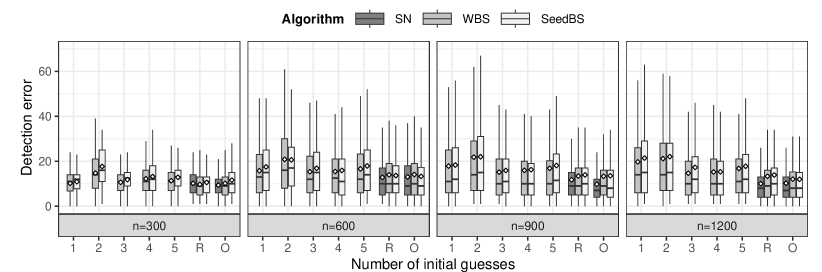
Figure D.1: Comparison of the modified two-step approach with multiple initial guesses ($1$-$5$), the Reliever method (R) and the original full model-fitting (O), under the setting in Section 4.1.

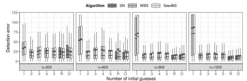
Figure D.2: Comparison of the modified two-step approach with multiple initial guesses ($1$-$5$), the Reliever method (R) and the original full model-fitting (O), under the setting in Section 4.2.

rss ref.bib

References

- Auger and Lawrence (1989) Auger, I. E. and Lawrence, C. E. (1989) Algorithms for the optimal identification of segment neighborhoods. Bull. Math. Biol., 51, 39–54.
- Bai and Perron (1998) Bai, J. and Perron, P. (1998) Estimating and testing linear models with multiple structural changes. Econometrica, 66, 47–78.
- Bai et al. (2023) Bai, P., Safikhani, A. and Michailidis, G. (2023) Multiple change point detection in reduced rank high dimensional vector autoregressive models. J. Amer. Statist. Assoc., To appear.
- Baranowski et al. (2019) Baranowski, R., Chen, Y. and Fryzlewicz, P. (2019) Narrowest-over-threshold detection of multiple change points and change-point-like features. J. R. Stat. Soc. Ser. B. Stat. Methodol., 81, 649–672.
- Chen and Chu (2023) Chen, H. and Chu, L. (2023) Graph-based change-point analysis. Annu. Rev. Stat. Appl., 10, 475–499.
- Chen et al. (2023) Chen, H., Ren, H., Yao, F. and Zou, C. (2023) Data-driven selection of the number of change-points via error rate control. J. Amer. Statist. Assoc., 118, 1415–1428.
- Cho and Kirch (2021) Cho, H. and Kirch, C. (2021) Data segmentation algorithms: Univariate mean change and beyond. Econom. Stat., To appear.
- Cho and Kirch (2022) — (2022) Two-stage data segmentation permitting multiscale change points, heavy tails and dependence. Ann. Inst. Statist. Math., 74, 653–684.
- Csörgő and Horváth (1997) Csörgő, M. and Horváth, L. (1997) Limit theorems in change-point analysis. John Wiley & Sons, Ltd., Chichester.
- Follain et al. (2022) Follain, B., Wang, T. and Samworth, R. J. (2022) High-dimensional changepoint estimation with heterogeneous missingness. J. R. Stat. Soc. Ser. B. Stat. Methodol., 84, 1023–1055.
- Frick et al. (2014) Frick, K., Munk, A. and Sieling, H. (2014) Multiscale change point inference. J. R. Stat. Soc. Ser. B. Stat. Methodol., 76, 495–580. With discussion.
- Friedman et al. (2010) Friedman, J. H., Hastie, T. and Tibshirani, R. (2010) Regularization paths for generalized linear models via coordinate descent. J. Stat. Softw., 33, 1–22.
- Fryzlewicz (2014) Fryzlewicz, P. (2014) Wild binary segmentation for multiple change-point detection. Ann. Statist., 42, 2243–2281.
- Haynes et al. (2017) Haynes, K., Fearnhead, P. and Eckley, I. A. (2017) A computationally efficient nonparametric approach for changepoint detection. Stat. Comput., 27, 1293–1305.
- Jackson et al. (2005) Jackson, B., Scargle, J. D., Barnes, D., Arabhi, S., Alt, A., Gioumousis, P., Gwin, E., Sangtrakulcharoen, P., Tan, L. and Tsai, T. T. (2005) An algorithm for optimal partitioning of data on an interval. IEEE Signal Proc. Let., 12, 105–108.
- Jewell et al. (2022) Jewell, S., Fearnhead, P. and Witten, D. (2022) Testing for a change in mean after changepoint detection. J. R. Stat. Soc. Ser. B. Stat. Methodol., 84, 1082–1104.
- Jiang et al. (2022) Jiang, F., Zhao, Z. and Shao, X. (2022) Modelling the COVID-19 infection trajectory: a piecewise linear quantile trend model. J. R. Stat. Soc. Ser. B. Stat. Methodol., 84, 1589–1607.
- Kaul et al. (2019a) Kaul, A., Jandhyala, V. K. and Fotopoulos, S. B. (2019a) Detection and estimation of parameters in high dimensional multiple change point regression models via regularization and discrete optimization. arXiv preprint, arXiv:1906.04396.
- Kaul et al. (2019b) — (2019b) An efficient two step algorithm for high dimensional change point regression models without grid search. J. Mach. Learn. Res., 20, 1–40.
- Killick et al. (2012) Killick, R., Fearnhead, P. and Eckley, I. A. (2012) Optimal detection of changepoints with a linear computational cost. J. Amer. Statist. Assoc., 107, 1590–1598.
- Kovács et al. (2022) Kovács, S., Li, H., Bühlmann, P. and Munk, A. (2022) Seeded binary segmentation: A general methodology for fast and optimal changepoint detection. Biometrika, To appear.
- Kovács et al. (2020) Kovács, S., Li, H., Haubner, L., Munk, A. and Bühlmann, P. (2020) Optimistic search: Change point estimation for large-scale data via adaptive logarithmic queries. arXiv preprint, arXiv:2010.10194.
- Lee et al. (2016) Lee, S., Seo, M. H. and Shin, Y. (2016) The lasso for high dimensional regression with a possible change point. J. R. Stat. Soc. Ser. B. Stat. Methodol., 78, 193–210.
- Leonardi and Bühlmann (2016) Leonardi, F. and Bühlmann, P. (2016) Computationally efficient change point detection for high-dimensional regression. arXiv preprint, arXiv:1601.03704.
- Li et al. (2022) Li, J., Fearnhead, P., Fryzlewicz, P. and Wang, T. (2022) Automatic change-point detection in time series via deep learning. arXiv preprint arXiv:2211.03860.
- Liu et al. (2021) Liu, L., Salmon, J. and Harchaoui, Z. (2021) Score-based change detection for gradient-based learning machines. In ICASSP 2021-2021 IEEE International Conference on Acoustics, Speech and Signal Processing (ICASSP), 4990–4994. IEEE.
- Londschien et al. (2022) Londschien, M., Bühlmann, P. and Kovács, S. (2022) Random forests for change point detection. arXiv preprint, arXiv:2205.04997.
- Londschien et al. (2021) Londschien, M., Kovács, S. and Bühlmann, P. (2021) Change-point detection for graphical models in the presence of missing values. J. Comput. Graph. Statist., 30, 768–779.
- Lu et al. (2017) Lu, Z., Banerjee, M. and Michailidis, G. (2017) Intelligent sampling for multiple change-points in exceedingly long time series with rate guarantees. arXiv preprint, arXiv:1710.07420.
- Niemiro (1992) Niemiro, W. (1992) Asymptotics for -estimators defined by convex minimization. Ann. Statist., 20, 1514–1533.
- Niu and Zhang (2012) Niu, Y. S. and Zhang, H. (2012) The screening and ranking algorithm to detect DNA copy number variations. Ann. Appl. Stat., 6, 1306–1326.
- Rinaldo et al. (2021) Rinaldo, A., Wang, D., Wen, Q., Willett, R. and Yu, Y. (2021) Localizing changes in high-dimensional regression models. In Proceedings of The 24th International Conference on Artificial Intelligence and Statistics, vol. 130, 2089–2097. PMLR.
- Wang et al. (2021a) Wang, D., Yu, Y. and Rinaldo, A. (2021a) Optimal change point detection and localization in sparse dynamic networks. Ann. Statist., 49, 203–232.
- Wang et al. (2021b) Wang, D., Zhao, Z., Lin, K. Z. and Willett, R. (2021b) Statistically and computationally efficient change point localization in regression settings. J. Mach. Learn. Res., 22, 1–46.
- Xu et al. (2022) Xu, H., Wang, D., Zhao, Z. and Yu, Y. (2022) Change point inference in high-dimensional regression models under temporal dependence. arXiv preprint, arXiv:2207.12453.
- Zou et al. (2014) Zou, C., Yin, G., Feng, L. and Wang, Z. (2014) Nonparametric maximum likelihood approach to multiple change-point problems. Ann. Statist., 42, 970–1002.