Nonparametric Bayesian approach for quantifying the conditional uncertainty of input parameters in chained numerical models

Abstract

Nowadays, numerical models are widely used in most of engineering fields to simulate the behaviour of complex systems, such as for example power plants or wind turbine in the energy sector. Those models are nevertheless affected by uncertainty of different nature (numerical, epistemic) which can affect the reliability of their predictions. We develop here a new method for quantifying conditional parameter uncertainty within a chain of two numerical models in the context of multiphysics simulation. More precisely, we aim to calibrate the parameters $\theta$ of the second model of the chain conditionally on the value of parameters $\lambda$ of the first model, while assuming the probability distribution of $\lambda$ is known. This conditional calibration is carried out from the available experimental data of the second model. In doing so, we aim to quantify as well as possible the impact of the uncertainty of $\lambda$ on the uncertainty of $\theta$. To perform this conditional calibration, we set out a nonparametric Bayesian formalism to estimate the functional dependence between $\theta$ and $\lambda$, denoted by $\theta(\lambda)$. First, each component of $\theta(\lambda)$ is assumed to be the realization of a Gaussian process prior. Then, if the second model is written as a linear function of $\theta(\lambda)$, the Bayesian machinery allows us to compute analytically the posterior predictive distribution of $\theta(\lambda)$ for any set of realizations $\lambda$. The effectiveness of the proposed method is illustrated on several analytical examples.

Keywords. Conditional Bayesian calibration, nonparametric regression, Gaussian process, empirical Bayes, cut-off models.

AMS classification: 60G15, 62G07, 62J05, 62F15.

1 Introduction

Over the last thirty years, numerical models have become important tools for modeling, understanding, analyzing and predicting the physical phenomena studied. In nuclear engineering, such models are essential because the physical experiments are often limited or even impossible for economic or ethical reasons (e.g., simulation of accidental transients for safety demonstration). The models, implemented to represent the physical reality faithfully, may depend on the specification of a large number of calibration parameters characterizing the studied phenomenon which are most often uncertain. Such parameters uncertainties are often due to a lack of knowledge of the phenomenon and, as a consequence, to some modeling assumptions. The process of quantifying parameter uncertainty according to the available experimental data is called model calibration. There are basically two types of calibration: deterministic calibration and calibration under uncertainties using Bayesian framework (Bayesian calibration) [21, 6, 12, 38, 41, 40]. Bayesian calibration allows us to quantify the parameter uncertainty by probability distribution instead of a single optimal value as in deterministic calibration. Such an optimal value is generally obtained by minimizing a criterion which quantifies a difference between the simulated data and the available experimental data (e.g., least square criterion).

This paper focuses on Bayesian calibration of models in the framework of multiphysics simulation. Multiphysics simulation refers to several numerical models of different physics which are connected to one another to simulate the entire phenomenon of interest. For example, in fuel simulation for nuclear power plants, the ALYCONE application is a multiphysics application [31]. It is composed of interdependent physical models that represent the mechanical, thermal and chemical behaviors of fuel rods in the core of pressurized water reactors. Among these different models, we will focus here on the thermal and the fission gas behavior models. The thermal model simulates the evolution of the temperature within the fuel rod during the fission reaction and provides as output, the associated temperature field. The fission gas behavior model, as a function of the thermal model, continuously represents the behavior of the fission products (fuel swelling and release of fission gas atoms) during the fission reaction.

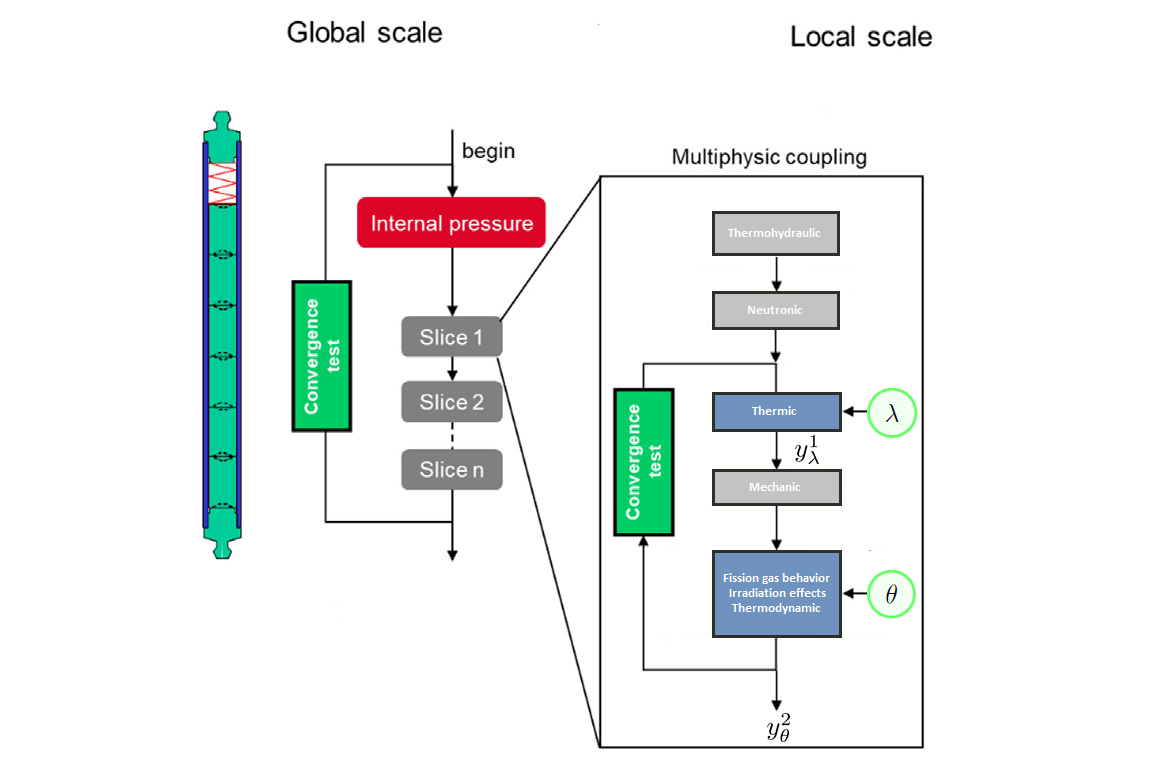
Figure 1: Chaining of the thermal and fission gas behavior models of the ALCYONE application [31]: $\lambda$ is the thermal conductivity and $\theta$ represents the parameters of the fission gas behavior model.

Figure 1 represents the chaining of these two models and their integration within the global calculation workflow. These models represented by blue boxes have as input parameters, respectively, the thermal conductivity $\lambda\in\mathbb{R}^{q}\,(q=1)$ and the parameters of the fission gas behavior model denoted $\theta\in\mathbb{R}^{p}\,(p\geq 1)$.

In the literature, two methods stand out for quantifying parameter uncertainties in interconnected models. First, we could calibrate $\theta$ of Model $2$ (fission gas behavior model in Figure 1) and $\lambda$ of Model $1$ (thermal model in Figure 1) independently of each other using experimental data from each phenomenon separately. Alternatively, we could opt for joint calibration using the whole set of data as proposed in [25], then enabling us to derive the posterior distribution of $\theta$ conditionally on $\lambda$. However, in this paper, our focus is only on the latter distribution given a prescribed marginal posterior distribution of $\lambda$, assumed accurate enough, thus eliminating the need for its re-estimation. Therefore, the approaches presented in [25] are not suitable in our context. Since a posterior probability density of $\theta$ given $\lambda$ is generally known upto a constant (unless for specific modeling assumptions), Markov chain Monte Carlo (MCMC) methods [36] are often necessary to sample it. Based on experimental data of Model $2$, a naive approach for the conditional calibration of $\theta$ given $\lambda$ would then be to run as many independent Markov chains as the number of $\lambda$ samples of interest. This approach is computationally expensive and omits that, under some regularity conditions, the conditional distribution $\theta|\lambda$ may give some informations about $\theta|\lambda^{\prime}$ if $\lambda$ is not too far from $\lambda^{\prime}$.

To overcome the above drawback, we propose a nonparameteric approach which directly learn the functional relation $\theta(\lambda)$ and infers its probability distribution. This approach is inspired by the work of [5] presented in another calibration context. The functional approach is based on the assumption that each component of $\theta(\lambda)$ is represented a priori as a trajectory of an independent Gaussian process. Moreover, it is implemented in the special case where the output of Model $2$ is assumed to be linear in $\theta$ given $\lambda$. The proposed method eventually provides a posterior predictive probability distribution of $\theta$ conditionally on any $\lambda$ and its feasibility is studied on analytical examples.

This paper is divided into five sections. In Section 2, we present a short state of the art of Bayesian calibration of numerical models. Section 3 is devoted to possible methods for conditional density estimation. In Section 4, we detail our approach, called GP-LinCC for Gaussian process and Linearization-based Conditional Calibration, and whose performances are illustrated in Section 5. Section 6 concludes the paper.

2 Bayesian calibration of numerical models

A physical system of interest $r(x)\in\mathcal{Y}\subset\mathbb{R}^{d^{\prime}}$ (here $d^{\prime}=1$) can be seen as a function describing the relationship between the input $x$ and the output of interest $r(x)$. The vector $x\in\mathcal{X}\subset\mathbb{R}^{d}$ is most often constituted of variables called control variables which typically represent experimental conditions and geometry of the physical system. Let $y_{\theta,\lambda}(x):=y^{2}_{\theta}(y^{1}_{\lambda}(x))$ be a deterministic numerical model resulting from the chaining of two physical models (like in Figure 1) and supposed to be representative of $r(x)$. Inspired by the work of [21], the experimental measurements $z=(z_{1},\cdots,z_{n})^{t}$ are related to the model outputs at the input values $(x_{i})_{i=1}^{n}$ by the following general probabilistic equation:

$$z_{i}=y_{\theta,\lambda}(x_{i})+b(x_{i})+\epsilon_{i},\,1\leq i\leq n,$$ (1)

where $\epsilon_{i}$ is the experimental uncertainty often considered as a realization of a zero-mean Gaussian distribution and the variance $\sigma^{2}_{\epsilon_{i}}$ is known. The unobserved term $b(x)$, called model discrepancy in [21], represents the gap between the numerical model $y_{\theta,\lambda}(x)$ and the physical system $r(x)$ when the model is run at the optimal value (or true) but unknown $(\theta,\lambda)$ of the uncertain parameters. The term $b(x)$ is often modeled by a Gaussian process [21, 2]. In the literature dedicated to Bayesian calibration, the term $b(x)$ is sometimes neglected and thus assumed to be indistinguishable from the experimental uncertainty [13]. Similarly, we will instead consider the simplified probabilistic equation:

$$z_{i}=y_{\theta,\lambda}(x_{i})+\epsilon_{i},\,1\leq i\leq n.$$ (2)

The joint posterior distribution is obtained by using Bayes’ formula:

$$\pi_{\text{full}}(\theta,\lambda|z)\propto\mathcal{L}(z|\theta,\lambda)\pi(\theta,\lambda),$$ (3)

where $\pi(\theta,\lambda)$ is the prior distribution quantiying the uncertainty of $(\theta,\lambda)$ before collecting the data $z$, $\mathcal{L}(z|\theta,\lambda)$ is the likelihood of the data $z$ conditionally on the couple $(\theta,\lambda)$ and the posterior distribution $\pi_{\text{full}}(\theta,\lambda|z)$ quantifies the residual uncertainty of $(\theta,\lambda)$ conditionally on $z$.

Sometimes, as in fuel simulation, there may be other sources of data which can bring information on some components of $(\theta,\lambda)$. In such cases, cut-off models can be used to properly partition the different sources of data that can provide information on the model parameters involved in the chaining [23, 33, 20]. Inspired by the work of [33], Figure 2 presents a cut-off model for the two chained physical models where the direct measurements $w$ (a realization of a some random variable $W$) bring information on $\lambda$ whereas the data $z$ (a realization of random variable $Z$) are seen by experts as uninformative on this parameter. More precisely, in Figure 2, the graph is divided by a cut into two subgroups (left and rigth of the dotted red line). The posterior distribution of $\lambda$ of the left subgroup is computed without considering the random variables of the right subgroup. Thus, the estimation of this posterior distribution is done only with the observation $w$ of W despite its possible dependence on $Z$. On the opposite, when estimating the posterior distribution of $\theta$ of the right subgroup, the terms of the left subgroup are taken into account.

Figure 2: Graphical representation of a cut-off model for two chained physical models. Single and double arrows give respectively stochastic and logical dependences. Square nodes are used for observed data.

Then, we can write the probability distribution of the parameters $(\theta,\lambda)$ conditionally on the complete data $(W=w,Z=z)$ as:

$$\pi_{\text{cut}}(\theta,\lambda|w,z)=\pi(\theta|\lambda,z)\pi(\lambda|w),$$ (4)

where $\pi(\lambda|w)\propto\mathcal{L}(w|\lambda)\pi(\lambda)$ is the posterior distribution when $w$ is observed only and $\pi(\theta|\lambda,z)$ is the posterior distribution of $\theta$ conditionally on $\lambda$. The distribution $\pi_{\text{cut}}(\theta,\lambda|w,z)$, called the cut distribution in [33], is different from the true joint posterior probability distribution $\pi_{\text{full}}(\theta,\lambda|w,z)$ which is written as:

$$\pi_{\text{full}}(\theta,\lambda|w,z)=\pi(\theta|\lambda,z)\pi(\lambda|w,z).$$ (5)

The two distributions are linked by the following relation:

$$\pi_{\text{cut}}(\theta,\lambda|w,z)\propto\frac{\pi_{\text{full}}(\theta,\lambda|w,z)}{\pi(z|\lambda)}.$$ (6)

Indeed, we have:

$$\pi_{\text{full}}(\theta,\lambda|w,z) =\frac{\mathcal{L}(z|\theta,\lambda)\pi(\theta|\lambda)\times\mathcal{L}(w|\lambda)\pi(\lambda)}{\pi(w,z)}$$ (7)

$$=\frac{\pi(\theta|\lambda,z)\pi(z|\lambda)\times\pi(\lambda|w)\pi(w)}{\pi(w,z)}$$ (8)

$$=\pi_{\text{cut}}(\theta,\lambda|w,z)\times\frac{\pi(z|\lambda)}{\pi(z|w)}.$$ (9)

In the sequel, the posterior distribution $\pi(\lambda|w)$ is assumed to be well-known and thus our goal comes down to estimating only the conditional posterior distribution $\pi(\theta|\lambda,z)$ in Equation (4). In the next section, we present some potential methods to achieve this goal.

3 Approaches for conditional density estimation

We aim to estimate the distribution of $\theta$ conditionally on any $\lambda$ varying in the support of $\pi(\lambda|w)$ and deduce an associated estimator for $\theta(\lambda)$. At first glance, one could use a kernel density estimator (KDE) [19, 32] to approximate the conditional posterior distribution $\pi(\theta|\lambda,z)$. This density estimator would require a large number $N$ of samples $\{\theta_{i},\lambda_{i}\}_{i=1}^{N}$ of $\pi_{\text{cut}}(\theta,\lambda|w,z)$ which could be generated by a Gibbs algorithm with possibly an inner Metropolis step (also called Metropolis-within-Gibbs) [36] as follows:

$$\theta_{i}\sim\pi_{\text{cut}}(\theta,\lambda_{i-1}|w,z)\propto\pi_{\text{full}}(\theta,\lambda_{i-1}|w,z)\,\text{(Equation \eqref{eq6})},$$ (10)

$$\lambda_{i}\sim\pi_{\text{cut}}(\lambda,\theta_{i}|w,z)\propto\frac{\pi_{\text{full}}(\theta_{i},\lambda|w,z)}{\pi(z|\lambda)},\,1\leq i\leq N.$$ (11)

However, in the general case, the marginal likelihood in the denominator of Equation (11) is computationally intractable

$$\pi(z|\lambda)=\int\mathcal{L}(z|\theta,\lambda)\pi(\theta|\lambda)d\theta.$$ (12)

As a result, the above sampling scheme is unfeasible because we are not able to sample the $\lambda_{i}$ according to Equation (11). Therefore, KDE-based appraoch could not be used with this sampling scheme to approximate $\pi(\theta|\lambda,z)$. Another solution may be for each $\lambda$ drawn in $\pi(\lambda|w)$, to use a Metropolis-Hastings algorithm (MH) [8] to approximate the associated conditional posterior distribution. More precisely, we would have the following MCMC sampling scheme:

$$\lambda_{i}\sim\pi(\lambda|w),$$ (13)

$$\theta_{i}\sim\pi(\theta|\lambda_{i},z),\,1\leq i\leq N.$$ (14)

However, if the numerical model is computationally expensive, this MH-based sampling scheme could not be repeated for a large number of different $\lambda$. This is why we can envisage to carry out this scheme by considering only a limited number $m$ of well-chosen values of $\lambda$, then using them to build a regression model to extrapolate the conditional distribution to another values of $\lambda$. This is presented hereafter.

3.1 Moment-based estimation method

We begin by creating a numerical design for $\lambda$, $D_{m}:=(\lambda_{1},\cdots,\lambda_{m})^{t}$ of size $m$ by Latin hypercube sampling [30] to spread out the samples in the support of the distribution $\pi(\lambda|w)$. Then, we estimate independently each conditional distribution $\pi(\theta|\lambda=\lambda_{j},z)$ for $j=1,\cdots,m$. Finally, we interpolate by a Gaussian process (GP) regression [34] the first two moments of the conditional posterior distribution of $\theta$ with respect to $D_{m}$ in order to predict them at new realizations $\lambda^{\star}\notin D_{m}$. More precisely, the steps are the following:

1. Creation of a numerical design $D_{m}$ according to $\pi(\lambda|w)$,

2. Computation of the $m$ conditional posterior distributions $\pi(\theta|\lambda_{j},z)$ by running a MH algorithm for each $1\leq j\leq m$. Let $(\theta^{j}_{i})_{i=1}^{N}$ be the resulting set of samples associated with $\lambda_{j}$ and generated from $\pi(\theta|\lambda_{j},z)$. The expectation and covariance matrix are then estimated by

   $$\bar{\theta}(\lambda_{j}):=\mathbb{E}(\theta|\lambda_{j},z)\approx\frac{1}{N}\sum_{i=1}^{N}\theta^{j}_{i},$$ (15)

   $$\operatorname{cov}(\theta|\lambda_{j},z)\approx\frac{1}{N}\sum_{i=1}^{N}(\theta^{j}_{i}-\bar{\theta}(\lambda_{j}))(\theta^{j}_{i}-\bar{\theta}(\lambda_{j}))^{t}.$$ (16)

3. Fitting of a GP model on the quantities (15) and (16) respectively based on their estimated values on $D_{m}$. From the two first moments learnt by the two GP, a Gaussian assumption is finally used to build a predictive distribution associated with any new realization $\lambda^{\star}\notin D_{m}$.

The main difficulty of Step $(iii)$ lies in preserving the positive semi-definite property of covariance matrices in the GP regression model. There are some solutions to satisfy this property:

• for $p=1$, GP regression on the log variance can be considered,

• for $p>1$, the solution proposed in [15] is to first carry out a regression on the Cholesky factors and then to use the inverse Cholesky decomposition to obtain predicted matrices ensuring the positive semi-definite property. However, this method is rather complex and omits any assessment of the prediction uncertainty.

To circumvent the use of an MH algorithm for estimating $\pi(\theta(\lambda)|z):=\pi(\theta|\lambda,z)$ in Step $(ii)$, we assume in the remainder of the paper that the output of the numerical model $y_{\theta,\lambda}(x)$ is linear in $\theta$ conditionally on $\lambda$. Regarding the fuel application which constitutes the applicative framework, the available simulations of the fission gas behavior model show that this linearity assumption is reasonable. With this assumption, Steps $(i)$ and $(ii)$ are easier to implement because MH sampling is not required anymore. However, the problem of interpolating covariance matrices remains. This is why we propose in the next section a new method for the approximation of $\pi(\theta(\lambda)|z)$ still under the framework of the linear assumption.

3.2 Proposed solution: method based on GP-prior and linear assumption (GP-LinCC method)

We aim to estimate the conditional posterior distribution $\pi(\theta|z,\lambda)$ for any realization $\lambda$. Our approach is to learn the relationship between $\theta$ and $\lambda$ through the function $\theta(\lambda)$ (called the calibration function) using the Bayesian paradigm based on three assumptions: a Gaussian process prior, the linearity of the output of the numerical model in $\theta(\lambda)$ and the compensation hypothesis that will be presented later (see Subsection 3.2.3).

3.2.1 Gaussian Process prior

Among the metamodels classically used for approximating computationally intensive numerical models, the GP regression is a powerful tool for nonparametric function metamodeling [37, 27]. The theory of GP is extensively detailed in [34] and more recently in [16]. Choosing it as a prior class of random functions (characterized by its mean and covariance functions) and conditioning on observed data yields a posterior GP which delivers a Gaussian predictive distribution for the model output at each prediction point with anaytical formulas for mean and covariance matrix [10] (see Appendix A.4). GP regression’s property of providing a predictive distribution (resulting in a probabilistic metamodel) rather than a simple predictor, largely explains its popularity, particularly in risk and safety assessment applications. Indeed, an uncertainty and confidence intervals can be derived for any quantity of interest estimated from the GP predictive distribution: estimation of a quantile, probability [29] or sensitivity indices [28, 22], performing an inversion problem [7], or construction of a sequential design of experiments [4, 16]. These properties have also been successfully used to emulate several chained (also called nested) or coupled codes, as in [25, 26] for calibration purpose.

In our case, we are quantifying the relationship between $\theta$ and $\lambda$ by learning the function $\theta(\lambda)\in\mathbb{R}^{p}$. We suppose each component of $\theta(\lambda)$ follows an independent GP which can be written as

$$\theta_{u}(\lambda)\overset{indep}{\sim}\mathcal{GP}\big{(}m_{\beta_{u}}(\lambda),\,\sigma_{u}^{2}K_{\psi_{u}}(\lambda,\,\lambda^{\prime})\big{)},\,1\leq u\leq p,$$ (17)

where $m_{\beta_{u}}(\lambda)$ is the mean function (also called trend) of the $u$-th GP which has to be specified or estimated. A constant $m_{\beta_{u}}(\lambda)=\beta_{u}$ or a one-degree polynomial trend is usually considered and recommended in practice. But any linear regression model on a set of known basis functions could be used instead. For simplicity, we will assume in the sequel that the prior mean is a constant $\beta_{u}$. The covariance function $\sigma_{u}^{2}K_{\psi_{u}}(\lambda,\,\lambda^{\prime})$ controls the regularity and scale of the trajectories of the GP ($\psi_{u}$ is the correlation length and $\sigma_{u}^{2}$ is the variance parameter). The covariance function $\sigma_{u}^{2}K_{\psi_{u}}(\lambda,\,\lambda^{\prime})$ is positive semi-definite and encodes the dependence structure of the $u$-th GP. One of the most popular choice of the covariance function is the Matérn $5/2$ covariance function, as recommended in [18], among others. The Matérn $5/2$ covariance function is given by:

$$\sigma_{u}^{2}K_{\psi_{u}}(\lambda,\,\lambda^{\prime})=\sigma_{u}^{2}\left(1+\sqrt{5}\frac{|\lambda-\lambda^{\prime}|}{{\psi_{u}}}+\frac{5}{3}{\frac{|\lambda-\lambda^{\prime}|}{{\psi_{u}}}}^{2}\right)e^{-\sqrt{5}\frac{|\lambda-\lambda^{\prime}|}{{\psi_{u}}}},$$ (18)

In the multidimensional case (i.e., $\lambda\in\mathbb{R}^{q},\,q\geq 1$), we can use a tensorization of $1$D-Matérn $5/2$ covariance function.

3.2.2 Linear case

The interest for a linear framework is that the posterior distribution of $\theta$ conditionally on $\lambda$ can be computed explicitly without any use of MCMC algorithms. We will consider that for any $\lambda$, the output of the numerical model $y_{\theta,\lambda}(x_{i})$ is linear in $\theta(\lambda)$. Thus, (2) becomes:

$$z_{i}=g_{\lambda,\,0}(x_{i})+g_{\lambda,\,1}(x_{i})^{t}\theta(\lambda)+\epsilon_{i},\,1\leq i\leq n,$$ (19)

where $\epsilon_{i}\sim\mathcal{N}(0,\sigma^{2}_{\epsilon_{i}}+\delta^{2}_{i})$ with $\delta^{2}_{i}$ being an extra scale parameter modelling the possible linearization error. In practice, the coefficients $g_{\lambda}(x_{i}):=\big{(}g_{\lambda,\,0}(x_{i}),\,g_{\lambda,\,1}(x_{i})\big{)}$ are often unknown and must be estimated by linearizing the code in $\theta(\lambda)$ at a fixed $(\lambda,x_{i})$. To perform the linearization, we fit for each $(\lambda_{j})_{j=1,\cdots,m}\in D_{m}$ and for each $x_{i}$, a linear regression from a set of training samples. More precisely, for each $(\lambda_{j})_{j=1,\cdots,m}$, a $n_{sim}$-size random sample of $\theta$ denoted $\Theta_{j}$ is generated and the corresponding simulations $y_{\Theta_{j},\,\lambda_{j}}(x_{i})$ are run. In the end, a total of $m\times n\times n_{sim}$ simulations are performed. Each set of the $n$ regression coefficients of these $m$ different linear regressions will constitute the estimates of the coefficients $(g_{\lambda_{j}}(x_{i}))_{i=1,\cdots,n}$ for each $(\lambda_{j})_{j=1,\cdots,m}\in D_{m}$.

3.2.3 Compensation hypothesis

In the context of the fuel application considered and introduced in Section 1, the compensation hypothesis is considered by experts as a necessary condition to address the problem of conditional calibration in a consistent way. This hypothesis states that the experimental data $z$ of the physical quantities of interest provide negligible information on the uncertainty of $\lambda$ (compared to that brought by $w$). And the same is desired for the corresponding simulated quantities $y^{2}_{\theta}(y^{1}_{\lambda}(x))$ with $x=(x_{1},\cdots,x_{n})^{t}$ (Figure 2). This means that $\pi(\lambda|z,w)$ must be as close as possible to $\pi(\lambda|w)$ in the sense of a dissimilarity measure (e.g. the Kullback-Leibler divergence). From Equations (4) and (5), this is equivalent to postulating that $\pi_{\text{cut}}(\theta,\lambda|z,w)$ is as close as possible to $\pi_{\text{full}}(\theta,\lambda|z,w)$, which happens when the ratio of the two marginal densities $\pi(z|w)$ and $\pi(z|\lambda)$ comes to $1$ (see Equation (9)). Therefore, this hypothesis will be satisfied if the likelihood of the data $z$ conditionally on the couple $(\theta,\lambda)$ is non-identifiable. That is to say that for any $\lambda\neq\lambda^{\prime}$, there would exist $\theta(\lambda)\neq\theta(\lambda^{\prime})$ giving the same likelihood [9].

4 GP-LinCC method: estimation and prediction

4.1 GP-LinCC method resulting from Gaussian process prior and Linearization

The combination of a Gaussian prior given by Equation (17) with a Gaussian likelihood due to the linearity hypothesis leads to an explicit posterior Gaussian distribution: we speak in this case of a conjugate family [35]. Thus, a Gaussian predictive distribution of $\theta$ conditionally on any $\lambda$ of non-zero probability with respect to $\pi(\lambda|w)$ is obtained, as detailed in Subsection 4.3.

4.2 GP-LinCC method in practice

To apply GP-LinCC method in practice to calibrate $\theta$ conditionally on $\lambda$, we need, in addition to the three basic assumptions described above (compensation, linearity of numerical model and GP prior), the following data:

• a set of experimental data noted $z$ of size $n$,

• a set of simulations of the numerical model $\{y_{\theta,\,\lambda}(x_{i})\}_{i=1,\cdots,n}$ for different values of $\lambda$ and $\theta$ to estimate the coefficients $(g_{\lambda}(x_{i}))_{i=1,\cdots,n}=\big{(}g_{\lambda,\,0}(x_{i}),\,g_{\lambda,\,1}(x_{i})\big{)}_{i=1,\cdots,n}$ of the linear model of Equation (19).

In the sequel, it is assumed that the coefficients of $(g_{\lambda}(x_{i}))_{i=1,\cdots,n}$ of the linear model of Equation (19) are well known and that $g_{\lambda,\,0}(x_{i})=0,$ $\forall\,\,1\leq i\leq n$.

4.3 Estimation: calculation of the posterior distribution

Equation (19) is applied to the $m$ realizations of $\lambda$ to learn the relation between $\theta$ and $\lambda$. Due to the compensation hypothesis presented above, we can then write $m$ equations involving the vector of experimental data $z=(z_{1},\cdots,z_{n})^{t}\in\mathbb{R}^{n}$:

$$z=g_{\lambda_{j}}(x)\theta(\lambda_{j})+\epsilon,\,1\leq j\leq m$$ (20)

where $g_{\lambda_{j}}(x):=\big{(}g_{\lambda_{j}}(x_{1})^{t},\cdots,g_{\lambda_{j}}(x_{n})^{t}\big{)}^{t}\in\mathbb{R}^{n\times p}$ and $\epsilon:=(\epsilon_{1},\cdots,\epsilon_{n})^{t}$. By summarizing these $m$ equations into a single matrix equation, we obtain:

$$\big{(}z,\cdots,z\big{)}=\big{(}g_{\lambda_{1}}(x)\theta(\lambda_{1}),\cdots,g_{\lambda_{m}}(x)\theta(\lambda_{m})\big{)}+\big{(}\epsilon,\cdots,\epsilon\big{)}.$$ (21)

Let $\mathbf{z}:=(z,\cdots,z)\in\mathbb{R}^{n\times m}$ be the matrix of the $m$ copies of $z$ and the associated macro parameter $\Theta_{m}:=\big{(}\theta(\lambda_{1}),\cdots,\theta(\lambda_{m})\big{)}^{t}\in\mathbb{R}^{m\times p}$. Each component of this macro parameter is a realization of a multivariate normal distribution according to Equation (17). Then, one way to infer the random matrix $\Theta_{m}$ is to work on the vectorized form of $\Theta_{m}$ noted $\vec{\Theta}_{m}\in\mathbb{R}^{pm}$ [3] (see Appendix A.3). Therefore, the prior distribution on $\Theta_{m}$ is written as:

$$\pi(\Theta_{m}|\phi)\propto|\textbf{K}_{\phi}|^{-\frac{1}{2}}\exp-\frac{1}{2}\big{(}\vec{\Theta}_{m}-\vec{M}_{\beta}\big{)}^{t}\textbf{K}_{\phi}^{-1}\big{(}\vec{\Theta}_{m}-\vec{M}_{\beta}\big{)},$$ (22)

where

$$\vec{M}_{\beta}=\big{(}m_{\beta_{1}}(\lambda_{1}),\cdots,m_{\beta_{p}}(\lambda_{1}),\cdots,m_{\beta_{1}}(\lambda_{m}),\cdots,m_{\beta_{p}}(\lambda_{m})\big{)}^{t}\in\mathbb{R}^{pm},$$

$$\textbf{K}_{\phi}=\{\operatorname{cov}\big{(}\theta(\lambda_{j}),\theta(\lambda_{j^{\prime}})\big{)}\}_{j,j^{\prime}=1}^{m},\text{ with }\operatorname{cov}\big{(}\theta(\lambda_{j}),\theta(\lambda_{j^{\prime}})\big{)}=\text{diag}\Big{\{}\sigma_{l}^{2}K_{\psi_{l}}(\lambda_{j},\,\lambda_{j^{\prime}})\Big{\}}_{l=1}^{p},$$

and $\phi:=(\beta_{l},\sigma^{2}_{l},\psi_{k})^{p}_{l=1}$. The expression of the likelihood of $\mathbf{z}$ conditionally on $\Theta_{m}$ is given by:

$$\mathcal{L}(\mathbf{z}|\Theta_{m}) =\mathcal{L}(z_{1}=z,\cdots,z_{m}=z|\theta(\lambda_{1}),\cdots,\cdots\theta(\lambda_{m}))$$ (23)

$$\propto\prod_{j=1}^{m}\exp-\frac{1}{2}\big{(}z-g_{\lambda_{j}}(x)^{t}\theta(\lambda_{j})\big{)}^{t}\Sigma_{\epsilon}^{-1}\big{(}z-g_{\lambda_{j}}(x)^{t}\theta(\lambda_{j})\big{)},$$ (24)

with $\Sigma_{\epsilon}:=\text{diag}(\sigma^{2}_{\epsilon_{1}}+\delta^{2}_{1},\cdots,\sigma^{2}_{\epsilon_{n}}+\delta^{2}_{n})$. Finally, the posterior probability distribution is given by the Bayes’ formula:

$$\pi(\Theta_{m}|\mathbf{z},\phi)\propto\mathcal{L}(\mathbf{z}|\Theta_{m})\pi(\Theta_{m}|\phi).$$ (25)

Theorem 1.

The posterior probability distribution $\pi(\Theta_{m}|\mathbf{z},\phi)$ is a multivariate normal distribution with mean $\mathbb{E}[\Theta_{m}|\mathbf{z},\phi]$ and covariance matrix $\mathbf{\Sigma}_{\phi}$ given below:

$$\mathbb{E}[\Theta_{m}|\mathbf{z},\phi]=\mathbf{\Sigma}_{\phi}\big{(}\textbf{K}_{\phi}^{-1}\vec{M}_{\beta}+G^{t}\Sigma_{\epsilon}^{-1}z\big{)}\in\mathbb{R}^{pm},$$ (26)

$$\mathbf{\Sigma}_{\phi}=\big{(}\mathbf{\Delta}^{-1}+\textbf{K}_{\phi}^{-1}\big{)}^{-1}\in\mathbb{R}^{pm\times pm},$$ (27)

where

$$G=(g_{\lambda_{1}}(x),\cdots,g_{\lambda_{m}}(x))\in\mathbb{R}^{n\times pm},$$

$$\mathbf{\Delta}^{-1}=\text{diag}\big{(}g_{\lambda_{1}}(x)^{t}\Sigma_{\epsilon}^{-1}g_{\lambda_{1}}(x),\cdots,g_{\lambda_{m}}(x)^{t}\Sigma_{\epsilon}^{-1}g_{\lambda_{m}}(x)\big{)}.$$

See Appendix B.1 for the proof of the theorem. From this posterior distribution, we can deduce a predictive distribution denoted $\pi_{pred}(\theta(\lambda^{\star})|\mathbf{z},\phi)$ associated with any new realization or set of realizations $\lambda^{\star}\notin D_{m}$.

4.4 Prediction: calculation of the predictive distribution

For any new set of realizations $\lambda^{\star}=(\lambda_{1}^{\star},\cdots,\lambda_{k}^{\star})^{t}$ belonging to the support of the distribution $\pi(\lambda|w)$, a predictive distribution of $\theta(\lambda^{\star})$ can be derived by integrating the conditional Gaussian distribution $\pi(\theta(\lambda^{\star})|\Theta_{m},\phi)$ over the posterior probability measure $\pi(\Theta_{m}|\mathbf{z},\phi)d\Theta_{m}$ given by Theorem 1:

$$\pi_{pred}(\theta(\lambda^{\star})|\mathbf{z},\phi)=\int\pi(\theta(\lambda^{\star})|\Theta_{m},\phi)\pi(\Theta_{m}|\mathbf{z},\phi)d\Theta_{m}.$$ (28)

Theorem 2.

The predictive distribution $\pi_{pred}(\theta(\lambda^{\star})|\mathbf{z},\phi)$ is a multivariate normal distribution with mean and covariance matrix respectively denoted by $\bar{\theta}_{pred}(\lambda^{\star})$ and $\Sigma_{pred}(\lambda^{\star},\lambda^{\star}{}^{\prime})$ such that

$$\bar{\theta}_{pred}(\lambda^{\star}):=\vec{m}_{\beta}(\lambda^{\star})+\mathbf{C}(\lambda^{\star},D_{m})\textbf{K}_{\phi}^{-1}\big{(}\mathbb{E}[\Theta_{m}|\mathbf{z},\phi]-\vec{M}_{\beta}\big{)},$$ (29)

$$\Sigma_{pred}(\lambda^{\star},\lambda^{\star}{}^{\prime}):=\mathbf{\Sigma}_{cond}(\lambda^{\star},\lambda^{\star}{}^{\prime})+\mathbf{C}(\lambda^{\star},D_{m})\textbf{K}_{\phi}^{-1}\,\mathbf{\Sigma}_{\phi}\,\textbf{K}_{\phi}^{-1}\mathbf{C}(D_{m},\lambda^{\star}{}^{\prime}),$$ (30)

where

$$\vec{m}_{\beta}(\lambda^{\star})=\big{(}m_{\beta_{1}}(\lambda^{\star}_{1}),\cdots,m_{\beta_{p}}(\lambda^{\star}_{1}),\cdots,m_{\beta_{1}}(\lambda^{\star}_{k}),\cdots,m_{\beta_{p}}(\lambda^{\star}_{k})\big{)}^{t}\in\mathbb{R}^{pk},$$

$$\mathbf{C}(\lambda^{\star},D_{m})=\big{\{}\operatorname{cov}\big{(}\theta(\lambda^{\star}_{i}),\theta(\lambda_{j})\big{)}\big{\}}_{1\leq i\leq k,1\leq j\leq m}\in\mathbb{R}^{pk\times pm},$$

$$\mathbf{\Sigma}_{cond}(\lambda^{\star},\lambda^{\star}{}^{\prime})=\mathbf{C}(\lambda^{\star},\lambda^{\star}{}^{\prime})-\mathbf{C}(\lambda^{\star},D_{m})\textbf{K}_{\phi}^{-1}\mathbf{C}(D_{m},\lambda^{\star}{}^{\prime})\in\mathbb{R}^{pk\times pk}.$$

The expression of $\bar{\theta}_{pred}(\lambda^{\star})$ corresponds to the classical expression of the mean of a conditional GP where the unknown quantity $\Theta_{m}$ is replaced by its posterior expectation $\mathbb{E}[\Theta_{m}|\mathbf{z},\phi]$. The mean $\bar{\theta}_{pred}(\lambda^{\star})$ is a predictor of $\theta(\lambda^{\star})$ which does not require the knowledge of $g_{\lambda^{\star}}(x_{i})_{i=1}^{n}$ for any $\lambda^{\star}$. The predictive covariance matrix $\Sigma_{pred}(\lambda^{\star},\lambda^{\star}{}^{\prime})$ is composed of two terms. The first one $\mathbf{\Sigma}_{cond}(\lambda^{\star},\lambda^{\star}{}^{\prime})$ corresponds to the classical formula for the covariance matrix of a conditional GP when $\Theta_{m}$ is known (we would have in this case $\Sigma_{pred}(\lambda^{\star},\lambda^{\star}{}^{\prime})=\mathbf{\Sigma}_{cond}(\lambda^{\star},\lambda^{\star}{}^{\prime})$). The additional term is related to the lack of knowledge of $\Theta_{m}$ conveyed by $\mathbf{\Sigma}_{\phi}$. Appendix (B.2) details the calculations of this predictive distribution.

All the previous formulas involve the hyperparameters $\phi$ which are never known in advance. We can estimate them either by likelihood maximization or by cross-validation [1]. This adds a preliminary step to enable us to evaluate the distributions of Theorems 1 and 2. In this paper, the hyperparameters $\phi$ are estimated by marginal likelihood maximization [34]. This technique, kwown as empirical Bayes, consists in maximizing the marginal likelihood in $\phi$ obtained by integrating the likelihood $\mathcal{L}(\mathbf{z}|\Theta_{m})$ over $\Theta_{m}$:

$$\widehat{\phi}:=\operatorname*{argmax}_{\phi}\int\mathcal{L}(\mathbf{z}|\Theta_{m})\pi(\Theta_{m}|\phi)d\Theta_{m}.$$ (31)

Finally, the accuracy of the predictive distribution in Theorem 2 can be evaluated by comparison with the distribution that we would obtain if using $g_{\lambda^{\star}}(x_{i})_{i=1}^{n}$ along with a Jeffreys prior on $\theta(\lambda^{\star})$. The expression of this distribution, called target distribution, is given by:

$$\pi_{target}(\theta(\lambda^{\star})|z\textbf{1}^{t}_{k})\sim\mathcal{N}_{pk}(\bar{\theta}_{target}(\lambda^{\star}),\Sigma_{target}(\lambda^{\star},{\lambda^{\star}}^{\prime})).$$ (32)

It is obtained from Theorem 1 where the matrix $\textbf{K}_{\phi}^{-1}$, the vector $\vec{M}_{\beta}$ and $m$ are replaced respectively by the null matrix of $\mathbb{R}^{pk\times pk}$, the null vector of $\mathbb{R}^{pk}$ and $k$. Another target distribution might be the one using $g_{\lambda^{\star}}(x_{i})_{i=1}^{n}$ along with a Gaussian prior whose hyperparameters are given by Equation (31):

$$\pi_{targetGP}(\theta(\lambda^{\star})|z\textbf{1}^{t}_{k},\hat{\phi})\sim\mathcal{N}_{pk}(\bar{\theta}_{targetGP}(\lambda^{\star}),\Sigma_{targetGP}(\lambda^{\star},{\lambda^{\star}}^{\prime})).$$ (33)

It is derived from Theorem 1 with $m=k$ and $\phi=\hat{\phi}$. The comparison between the three distributions (predictive and the two targets) will be done via the MSE criterion described in the next section.

4.5 Accuracy criterion: MSE

The criterion we consider is the mean square error (MSE). It is calculated by integrating over $\pi(\lambda|w)$ the difference between the true value $\theta(\lambda)$ and the mean predictor $\bar{\theta}_{pred}(\lambda)$ (respectively $\bar{\theta}_{target}(\lambda)$, $\bar{\theta}_{targetGP}(\lambda)$ for the target distributions):

$$\text{MSE}=\int(\theta(\lambda)-\bar{\theta}_{pred}(\lambda))^{t}(\theta(\lambda)-\bar{\theta}_{pred}(\lambda))\pi(\lambda|w)d\lambda.$$ (34)

In practice, it is approximated by a Monte Carlo estimator:

$$\frac{1}{N_{\lambda}}\sum_{j=1}^{N_{\lambda}}(\theta(\lambda_{j})-\bar{\theta}_{pred}(\lambda_{j}))^{t}(\theta(\lambda_{j})-\bar{\theta}_{pred}(\lambda_{j})),$$ (35)

where $(\lambda_{j})_{j=1,\cdots,N_{\lambda}}$ are a $N_{\lambda}$-size sample of i.i.d. realizations of $\lambda$. The lower the MSE, the more accurate the predictor $\bar{\theta}_{pred}(\lambda)$. In the numerical examples, we will consider an empirical MSE for each component $\theta_{u}(\lambda)$ of $\theta(\lambda)$:

$$\text{MSE}_{u}\approx\frac{1}{N_{\lambda}}\sum_{j=1}^{N_{\lambda}}(\theta_{u}(\lambda_{j})-\bar{\theta}_{pred_{u}}(\lambda_{j}))^{2},\,1\leq u\leq p\,\text{ (and resp. for $\bar{\theta}_{target}(\lambda)$, $\bar{\theta}_{targetGP}(\lambda)$)}.$$ (36)

Afterwards, we can check to which extend the calibrated model $\{g_{\lambda}(x_{i})^{t}\bar{\theta}_{pred}(\lambda)\}_{1\leq i\leq n}$ is constant in $\lambda$ (in other words whether the compensation hypothesis is verified).

4.6 A test for checking the compensation hypothesis

The compensation hypothesis states that the predictions of the numerical model should be constant in $\lambda$. To inspect this hypothesis, we compute the predictive distribution of the numerical model associated to each $\lambda$:

$$\pi(g_{\lambda}(x)\theta(\lambda)|\mathbf{z},\lambda,\phi)\sim\mathcal{N}_{n}(g_{\lambda}(x)\bar{\theta}_{pred}(\lambda),\,g_{\lambda}(x)\Sigma_{pred}(\lambda,\lambda^{\prime})g_{\lambda}(x)^{t}).$$ (37)

By integrating over the whole uncertainty of $\lambda$, we have:

$$\pi(g_{\lambda}(x)\theta(\lambda)|\mathbf{z},\phi)=\int\pi(g_{\lambda^{\prime}}(x)\theta(\lambda^{\prime})|\mathbf{z},\phi,\lambda^{\prime})\pi(\lambda^{\prime}|w)d\lambda^{\prime}.$$ (38)

Using the cross-validation technique [19, 1], we can derive for any configuration $x_{i}$, the predictive distribution of the associated numerical model for any $\lambda$, for $1\leq i\leq n$:

$$\pi(g_{\lambda}(x_{i})^{t}\theta(\lambda)|\mathbf{z}_{-i},\lambda,\phi)\sim\mathcal{N}\big{(}g_{\lambda}(x_{i})^{t}\bar{\theta}_{pred,-i}(\lambda),g_{\lambda}(x_{i})^{t}\Sigma_{pred,-i}(\lambda,\lambda)g_{\lambda}(x_{i})\big{)},$$ (39)

where $\mathbf{z}_{-i}$ is equal to $\mathbf{z}$ without the column $i$, $\bar{\theta}_{pred,-i}$ and $\Sigma_{pred,-i}$ are given by Theorem 2 where $\mathbf{z}$ is replaced by $\mathbf{z}_{-i}$. If the compensation hypothesis is achieved by the numerical model, then for any $\lambda_{1}\neq\lambda_{2}$, the distributions $\pi(g_{\lambda_{1}}(x_{i})^{t}\theta(\lambda_{1})|\mathbf{z}_{-i},\lambda_{1})$, $\pi(g_{\lambda_{2}}(x_{i})^{t}\theta(\lambda_{2})|\mathbf{z}_{-i},\lambda_{2})$ and $\pi(g_{\lambda}(x_{i})^{t}\theta(\lambda)|\mathbf{z}_{-i},\phi)$ are expected to be similar to each other. Thus the predictive credibility interval of the distribution of the random variable

$$g_{\lambda_{1}}(x_{i})^{t}\theta(\lambda_{1})-g_{\lambda}(x_{i})^{t}\theta(\lambda_{2})|\mathbf{z}_{-i},\lambda_{1},\lambda_{2},\phi$$ (40)

is likely to cover $0$. This random variable follows a normal distribution of mean and variance given respectively by:

$$\mu_{i}(\lambda_{1},\lambda_{2}) :=g_{\lambda_{1}}(x_{i})^{t}\bar{\theta}_{pred,-i}(\lambda_{1})-g_{\lambda_{2}}(x_{i})^{t}\bar{\theta}_{pred,-i}(\lambda_{2}),$$

$$\sigma^{2}_{i}(\lambda_{1},\lambda_{2}) :=g_{\lambda_{1}}(x_{i})^{t}\Sigma_{pred,-i}(\lambda_{1},\lambda_{1})g_{\lambda_{1}}(x_{i})-2g_{\lambda_{1}}(x_{i})^{t}\Sigma_{pred,-i}(\lambda_{1},\lambda_{2})g_{\lambda_{2}}(x_{i})$$

$$+g_{\lambda_{2}}(x_{i})^{t}\Sigma_{pred,-i}(\lambda_{2},\lambda_{2})g_{\lambda_{2}}(x_{i}).$$

From this distribution, we can compute an empirical coverage probability for $0$ for $1-\alpha$ level, from $N$ different i.i.d. sample pairs $(\lambda_{1},\lambda_{2})\sim\pi(\lambda|w)\times\pi(\lambda|w)$:

$$\hat{\Delta}(\alpha,x_{i})=\frac{1}{N}\sum_{j=1}^{N}\textbf{1}_{\big{\{}0\in\big{[}\mu_{i}(\lambda^{j}_{1},\lambda^{j}_{2})\pm q_{1-\frac{\alpha}{2}}\sqrt{\sigma^{2}_{i}(\lambda^{j}_{1},\lambda^{j}_{2})}\big{]}\big{\}}}$$ (41)

where $q_{1-\frac{\alpha}{2}}$ is the $(1-\frac{\alpha}{2})$ quantile of the standard Gaussian distribution. The objective is to obtain $\hat{\Delta}(\alpha,x_{i})$ as close as possible to the theoretical probability of interval $1-\alpha$. For instance, considering a standard level $\alpha=5\%$, if the coverage probability $\hat{\Delta}(5\%,x_{i})$ is lower than $95\%$, then the compensation hypothesis must be questioned.

5 Numerical examples

5.1 Example $1$ in $1$D $(\theta\in\mathbb{R})$

We consider the following probabilistic model:

$$z_{i}=r+\epsilon_{i},\,1\leq i\leq n,$$ (42)

where $\epsilon_{i}\sim\mathcal{N}(0,2)$ and the chosen $r$ system is assumed to be constant and equal to $5$. We model it by

$$y_{\theta,\lambda}=\lambda\theta,$$ (43)

where

$$\pi(\lambda|w)\sim\mathcal{U}[1,\,10],$$ (44)

Equation (42) can thus be rewritten as,

$$z_{i}=\lambda\theta+\epsilon_{i},\,1\leq i\leq n.$$ (46)

The prior distribution on $\Theta_{m}$ is chosen with:

• a Matérn $5$/$2$ covariance function given by Equation (18),

• a constant mean function: $m_{\beta}(\lambda)=\beta$.

A Latin hypercuble sampling (LHS) [30] is used to sample $\lambda\sim\pi(\lambda|w)$ and generate the design $D_{m}$. The GP hyperparameters $\phi=(\beta,\psi,\sigma^{2})$ are estimated by marginal likelihood maximization (Equation (31)). Appendix B.3 details this estimation. Once $\phi$ is estimated and denoting $\hat{\phi}$ its estimator, the predictive distribution $\pi_{pred}(\theta(\lambda^{\star})|z\textbf{1}^{t},\hat{\phi})$ is computed for a vector $\lambda^{\star}\in[1,10]^{k}$ with $k$ new realizations, and then compared to the target distribution $\pi_{target}(\theta(\lambda^{\star})|z\textbf{1}^{t}_{k})$. Figure 3 presents the results obtained with $n=50$ i.i.d. samples generated by Equation (42) , $m=10$ and $k=500$. On this figure, we have printed the true function $\theta(\lambda)=\frac{r}{\lambda}$ as well as the means of the predictive and target distributions denoted respectively by $\bar{\theta}_{pred}(\lambda)$ and $\bar{\theta}_{target}(\lambda)$. The $95\%$ credibility intervals associated with these two distributions are also represented. It can be seen that the predicted mean $\bar{\theta}_{pred}(\lambda)$ is relatively close to both the true and target functions and that the predicted credibility intervals of $95\%$ cover them relatively well. We have not plotted $\bar{\theta}_{targetGP}(\lambda)$ (respectively its credibility interval of $95\%$). In fact, we can easily notice that $\bar{\theta}_{targetGP}(\lambda)$ and $\Sigma_{targetGP}(\lambda,\lambda)$ are very close to $\bar{\theta}_{target}(\lambda)$ and $\Sigma_{target}(\lambda,\lambda)$ respectively because the estimated variance $\hat{\sigma}^{2}$ of the GP is greater than $\Sigma_{target}(\lambda,\lambda)$. These quantities are related by

$$\Sigma_{targetGP}(\lambda,\lambda)=\frac{\Sigma_{target}(\lambda,\lambda)}{1+\frac{\Sigma_{target}(\lambda,\lambda)}{\hat{\sigma}^{2}}}\approx\frac{\sigma^{2}_{\epsilon}}{n\lambda^{2}}$$ (47)

$$\bar{\theta}_{targetGP}(\lambda)=\frac{\sigma^{2}_{\epsilon}}{\sigma^{2}_{\epsilon}+n\lambda^{2}\hat{\sigma}^{2}}\hat{\beta}+\frac{\bar{z}}{\lambda}\frac{1}{1+\frac{\sigma^{2}_{\epsilon}}{n\lambda^{2}\hat{\sigma}^{2}}}\approx\bar{\theta}_{target}(\lambda)$$ (48)

where $\Sigma_{target}(\lambda,\lambda)=\frac{\sigma^{2}_{\epsilon}}{n\lambda^{2}}=\frac{2}{n\lambda^{2}}$, $\bar{\theta}_{target}(\lambda)=\frac{\bar{z}}{\lambda}$, $\hat{\sigma}^{2}=8.72$, $\hat{\beta}=2.98$.

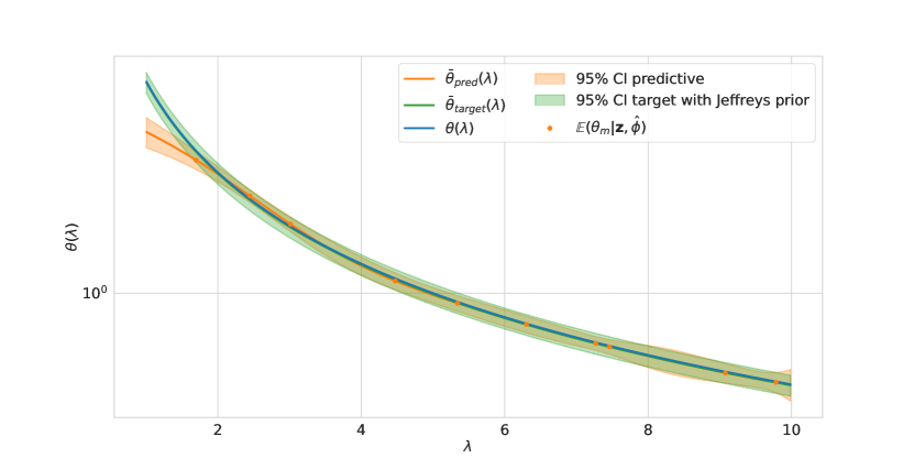
Figure 3: True function $\theta(\lambda)$, predicted mean denoted by $\bar{\theta}_{pred}(\lambda)$, target mean denoted by $\bar{\theta}_{target}(\lambda)$ (with Jeffreys prior) and associated $95\%$ credibility intervals, obtained from a sample of $n=50$ observations and a design $D_{m}$ with $m=10$. The $y$-axis is in log-scale.

For a given vector $\lambda^{\star}\in[1,10]^{N_{\lambda}}$ with ${N_{\lambda}}=1000$ new i.i.d. realizations of $\lambda$, we have computed the empirical MSE of the following estimators:

• $\bar{\theta}_{pred}(\lambda^{\star})$ the mean of the predictive distribution given by Theorem 2 with $p=1$,

• $\bar{\theta}_{target}(\theta(\lambda^{\star})|z)$ the mean of the target distribution with Jeffreys prior given by 32 with $p=1$,

• $\bar{\theta}_{targetGP}(\lambda^{\star})$ the mean of the target distribution with a Gaussian prior on $\theta(\lambda^{\star})$ whose hyperparameters are estimated from $D_{m}$ and $z$. It is given by Equation (33) with $p=1$.

This procedure is randomly replicated $100$ times for two sample sizes $n\in\{50,100\}$ of observations $z$ and three sample sizes $m\in\{10,15,20\}$ of $D_{m}$. Each replication is performed from independent samples of $z$ and independent LHS designs $D_{m}$. Figure 4 shows the boxplots of the empirical MSE thus obtained. For both sample sizes $n$, two phenomena are observed as $m$ increases:

• the boxplot of the empirical MSE of $\bar{\theta}_{pred}(\lambda^{\star})$ comes close to that of $\bar{\theta}_{targetGP}(\lambda^{\star})$,

• the results obtained for the two target distributions but calculated with two different priors differ little. The impact of the prior choice is therefore limited in this case, mostly due to the use of empirical Bayes.

Figure 4: Boxplots of the MSE of the means of predictive and target distributions for observations samples of size $n\in\{50,100\}$ and from a design $D_{m}$ with $m\in\{10,15,20\}$ replicated $100$ times.

5.2 Example $2$ in $2$D $(\theta\in\mathbb{R}^{2})$

We consider the following analytical example:

• an additive physical system of interest: $r(x)=r_{1}(x)+r_{2}(x)$ avec $r_{1}(x)\neq r_{2}(x)\,\,\forall\,x\in[-4,\,4]$,

• the experimental data are linked to the system via:

  $$z_{i}=r(x_{i})+\epsilon_{i},\,-4\leq x_{i}\leq 4,\,i=1,\cdots,n,$$ (49)

  $$\epsilon_{i}\sim\mathcal{N}(0,\sigma^{2}_{\epsilon_{i}}),\,\sigma^{2}_{\epsilon_{i}}:=(0.06|r(x_{i})|)^{2}.$$ (50)

We postulate the following linear numerical model, supposed to represent $r(x)$ and verifying the compensation hypothesis:

$$r(x_{i})=g_{\lambda}(x_{i})^{t}\theta(\lambda),\,\theta(\lambda)\in\mathbb{R}^{2},$$ (51)

where the components of $\theta(\lambda)$ are given by:

$$\theta_{1}(\lambda)=\lambda\sin(10\lambda)+1,\,\theta_{2}(\lambda)=\sin(2\pi\lambda/10)+0.2\sin(20\pi\lambda/2.5)+1.75,$$ (52)

and $\pi(\lambda|w)\sim\mathcal{U}[0,\,1]$. The two functions $\theta_{l}(\lambda)_{l=\{1,2\}}$ are chosen from [39]. We need to construct $g_{\lambda}(x_{i})$ in such a way that the numerical model $g_{\lambda}(x_{i})^{t}\theta(\lambda)$ remains unchanged in $\lambda$. To do this, we propose to set:

$$g_{1}(x_{i},\lambda)=\frac{r_{1}(x_{i})}{\theta_{1}(\lambda)}=\frac{x_{i}^{2}+x_{i}+1}{\theta_{1}(\lambda)}\,\text{and }g_{2}(x_{i},\lambda)=\frac{r_{2}(x_{i})}{\theta_{2}(\lambda)}=\frac{x_{i}^{2}+x_{i}+4}{\theta_{2}(\lambda)}.$$ (53)

With this choice, the compensation hypothesis is verified and moreover, the matrix $\mathbf{\Delta}$ of Theorem 1 is invertible. The prior distribution on $\Theta_{m}$ is chosen from two GP prior for $\theta_{1}(\lambda)$ and $\theta_{2}(\lambda)$ with for each:

• a Matérn 5/2 covariance function given by Equation (18),

• a constant mean function: $m_{\beta_{l}}(\lambda)=\beta_{l},\,l\in\{1,\,2\}$.

Once $\phi=(\beta_{l},\sigma^{2}_{l},\psi_{l})_{1\leq l\leq 2}$ is estimated, the predictive distribution $\pi_{pred}(\theta(\lambda^{\star})|\mathbf{z},\hat{\phi})$ is computed for a vector $\lambda^{\star}\in[1,10]^{k}$ with $k=500$ new realizations, then compared to the target distribution $\pi_{target}(\theta(\lambda^{\star})|z\textbf{1}^{t}_{k})$. Figures 5 (a) and (b) present respectively the two components $\theta_{1}(\lambda)$ et $\theta_{2}(\lambda)$ of the true function $\theta(\lambda)$ as well as the two means of both the predictive and target distributions calculated with a sample of $n=50$ i.i.d. observations generated by Equation (49) and a design $D_{m}$ of size $m=10$. The $95\%$ credibility intervals cover relatively well the two components of the true function ((a) for $\theta_{1}(\lambda)$ and (b) for $\theta_{2}(\lambda)$). We also observe that the marginal predictors are able to approximate well the components of the true function and those of the target function. Figure 6 presents the comparison between the marginal predictive and target densities for a specific $\lambda^{\star}$, equal to 0.45. For this $\lambda$ realization, the three densities are in good agreeement.

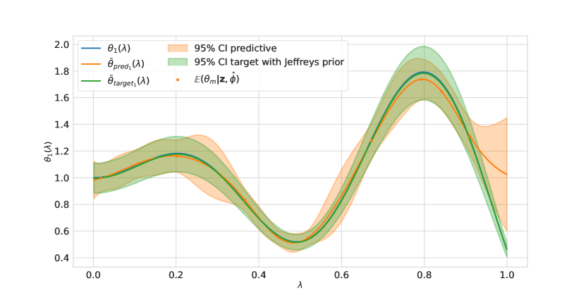
(a)

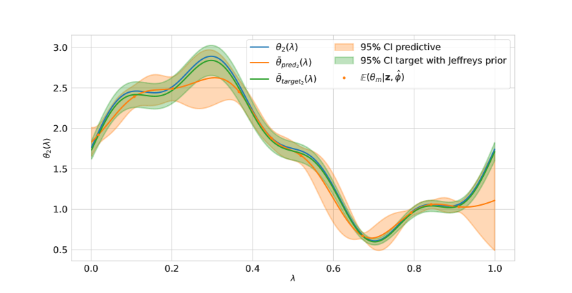
(b)

Figure 5: Comparison of the three functions $\theta(\lambda),\,\bar{\theta}_{pred}(\lambda)$ and $\bar{\theta}_{target}(\lambda)$, for the two components of $\theta(\lambda)$.

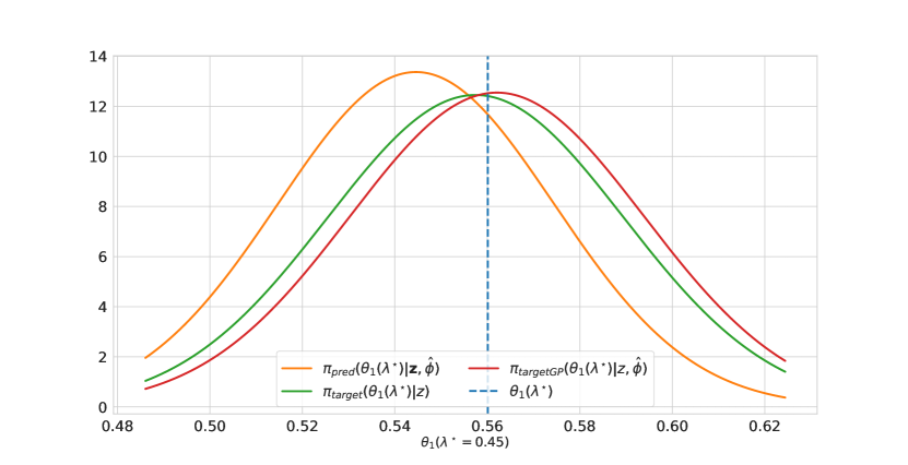
(a)

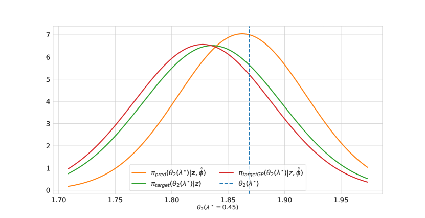
(b)

Figure 6: Comparison of the three marginal probability densities obtained from a sample of $n=50$ observations and $D_{m}$ with $m=10$.

For a given vector $\lambda^{\star}\in[1,10]^{N_{\lambda}}$ with $N_{\lambda}=1000$ new i.i.d. realizations of $\lambda$, we have computed the empirical MSE of the following estimators:

• $\bar{\theta}_{pred}(\lambda^{\star})$ the mean of the predictive distribution given by Theorem 2 with $p=2$,

• $\bar{\theta}_{target}(\lambda^{\star})$ the mean of the target distribution with Jeffreys prior given by Equation (32) with $p=2$,

• $\bar{\theta}_{targetGP}(\lambda^{\star})$ the mean of the target distribution with a Gaussian prior on $\theta(\lambda^{\star})$ whose hyperparameters are estimated from $D_{m}$ and $z$. It is given by Equation (33) with $p=2$.

This procedure is randomly replicated $100$ times for two sample sizes $n\in\{50,100\}$ of observations $z$ and three sample sizes $m\in\{10,15,20\}$ of $D_{m}$. Results are given by Figures 7 and 8, for $\theta_{1}(\lambda)$ and $\theta_{2}(\lambda)$ respectively. We can see that for $m=10$, the GP-LinCC method predicts better the first component than the second one. This could be due to the shape of these two components. However, when $m$ increases, it predicts well the components of $\theta(\lambda)$.

Figure 7: Boxplots of the MSE of the first marginal predictive and both target distributions for a design $D_{m}$ of size $m\in\{10,15,20\}$ and a sample of size $n\in\{50,100\}$ of the observations replicated $100$ times.

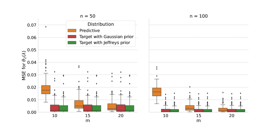
Figure 8: Boxplots of the MSE of the second marginal predictive and both target distributions for a design $D_{m}$ of size $m\in\{10,15,20\}$ and a sample of size $n\in\{50,100\}$ of the observations repeated $100$ times.

5.3 Example $3$ in $1$D $(\theta\in\mathbb{R})$ with falsification of the compensation hypothesis

In this example, we will test the GP-LinCC method in the case where the compensation hypothesis is violated. The sampling of experimental data now depends on $\lambda$. We have chosen a specific sample $\lambda_{0}$ such that:

$$z_{i}=r_{\lambda_{0}}(x_{i})+\epsilon_{i},\,1\leq i\leq n,$$ (54)

$$z_{i}=g_{\lambda_{0}}(x_{i})^{t}\theta(\lambda_{0})+\epsilon_{i},\,1\leq i\leq n,$$ (55)

with $r_{\lambda}$ not being equal to $r_{\lambda_{0}}$ if and only if $\lambda$ is not equal to $\lambda_{0}$. For any $\lambda$, the observations $z$ can actually be related to the numerical model outputs via:

$$z_{i}=g_{\lambda}(x_{i})^{t}\theta(\lambda)+b(x_{i},\lambda)+\epsilon_{i},\,1\leq i\leq n,$$ (56)

where the discrepancy term $b(x_{i},\lambda)$ is equal to:

$$b(x_{i},\lambda) =g_{\lambda_{0}}(x_{i})^{t}\theta(\lambda_{0})-g_{\lambda}(x_{i})^{t}\theta(\lambda)=g_{\lambda}(x_{i})^{t}\big{(}\frac{g_{\lambda_{0}}(x_{i})^{t}\theta(\lambda_{0})}{g_{\lambda}(x_{i})^{t}\theta(\lambda)}-1\big{)}\theta(\lambda)$$ (57)

$$=(\alpha(x_{i},\lambda)-1)g_{\lambda}(x_{i})^{t}\theta(\lambda),$$ (58)

where

$$\alpha(x_{i},\lambda)=\frac{g_{\lambda_{0}}(x_{i})^{t}\theta(\lambda_{0})}{g_{\lambda}(x_{i})^{t}\theta(\lambda)}=\frac{r_{\lambda_{0}}(x_{i})}{r_{\lambda}(x_{i})}.$$ (59)

Equation (56) becomes:

$$z_{i}=g_{\lambda}(x_{i})^{t}\alpha(x_{i},\lambda)\theta(\lambda)+\epsilon_{i},\,1\leq i\leq n.$$ (60)

As $\alpha(x_{i},\lambda)$ is neglected by the GP-LinCC method, the mean estimators $\bar{\theta}_{pred}(\lambda)$ are equal to $\bar{\theta}_{target}(\lambda)=(g_{\lambda}(x)^{t}g_{\lambda}(x))^{-1}g_{\lambda}(x)^{t}z$. By propagating these estimators through the model, we obtain the following calibrated predictions that depend on $\lambda$:

$$\widehat{r}_{\lambda}(x_{i}):=g_{\lambda}(x_{i})^{t}\bar{\theta}_{pred}(\lambda),\ 1\leq i\leq n\Longrightarrow\widehat{r}_{\lambda}(x)=g_{\lambda}(x)\bar{\theta}_{pred}(\lambda).$$ (61)

For our test case, we choose the following physical system

$$r_{\lambda}(x_{i})=3x_{i}^{2}+2\lambda^{2}x_{i}+1+\lambda,\,-2\leq x_{i}\leq 2,$$ (62)

$\pi(\lambda|w)\sim\mathcal{U}[0,\,1]$ and the numerical model $g_{\lambda}(x)\theta(\lambda)$ such that

$$g_{\lambda}(x_{i})=\frac{r_{\lambda}(x_{i})}{\theta(\lambda)},\theta(\lambda)=1+\lambda\sin(10\lambda).$$ (63)

The i.i.d. observations $z=(z_{1},\cdots,z_{n})^{t}$ are generated with $\lambda_{0}=0.5$ and the variance $\sigma^{2}_{i}=0.06(r_{\lambda_{0}}(x_{i}))^{2}$ for $1\leq i\leq n$ by Equation (54). Once $\phi=(\beta_{l},\sigma^{2}_{l},\psi_{l})_{1\leq l\leq 2}$ is estimated, the predictive distribution is computed for a vector $\lambda^{\star}\in[1,10]^{k}$ with $k=500$ new realizations, then compared to the target distribution $\pi_{target}(\theta(\lambda^{\star})|z\textbf{1}^{t}_{k})$. Figure 9 presents the true function $\theta(\lambda)$, the predicted function $\bar{\theta}_{pred}(\lambda)$ and the target function $\bar{\theta}_{target}(\lambda)$ computed from a sample of $z$ and a design $D_{m}$ of size $m=10$, as well as the associated $95\%$ credibility intervals. We can see that the predicted function does not match the true function whereas, as expected, it approximates well the target function. The predictors $\widehat{r}_{\lambda}(x)$ for different $\lambda$ and the physical system $r_{\lambda_{0}}(x)$ are plotted in Figure 10 where we can observe that these predictors vary with the chosen value of $\lambda$. This reveals that the calibrated model does not compensate in $\lambda$. This absence of compensation is also confirmed by the predictive distributions $\pi(g_{\lambda_{j}}(x_{i})^{t}\theta(\lambda)|\mathbf{z}_{-i},\lambda_{j},\hat{\phi}),\,x_{i}\in\{x_{1},x_{4}\}$ for $1\leq j\leq 4$ as presented in Figure 11. The empirical coverage probabilities $\hat{\Delta}(5\%,x_{i})$, computed with $N=5000$ pairs of samples $(\lambda_{1},\lambda_{2})$, presented in Figure 12 do not exceed the threshold of $95\%$, revealing once again that the compensation hypothesis is not satisfied. These results are coherent with the simulation procedure of the observations $z$. Indeed, since $z$ has been simulated with a nominal value $\lambda_{0}=0.5$, the predicted function $\theta_{pred}(\lambda)$ is not able to predict well the true function for new realizations of $\lambda$ not close to $\lambda_{0}$. This can be observed in Figure 9.

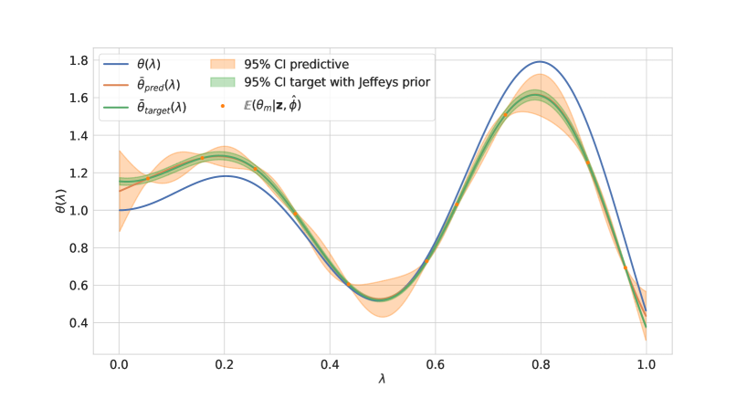
Figure 9: True function $\theta(\lambda)$, predicted mean noted $\bar{\theta}_{pred}(\lambda)$, target mean noted $\bar{\theta}_{target}(\lambda)$ and associated $95\%$ credibility intervals, obtained with a sample of $n=50$ observations and a design $D_{m}$ of size $m=10$.

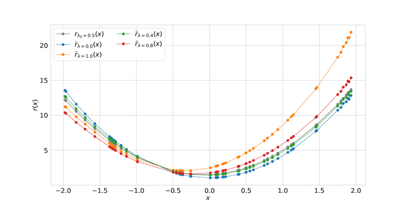
Figure 10: Predictors $\widehat{r}_{\lambda}(x)$ for different values of $\lambda$ compared to $r_{\lambda_{0}}(x)$.

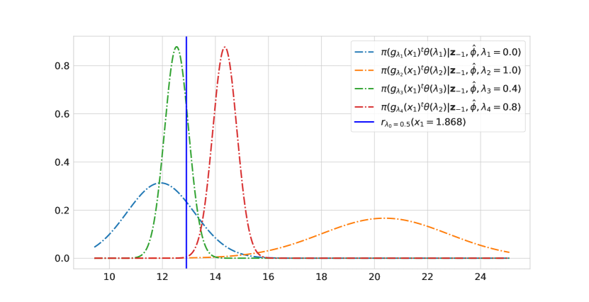
(a)

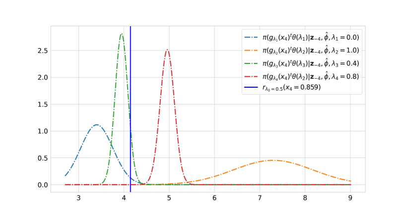
(b)

Figure 11: Predictive densities $\pi(g_{\lambda_{j}}(x_{i})^{t}\theta(\lambda)|\mathbf{z}_{-i},\lambda_{j},\hat{\phi}),\,x_{i}\in\{x_{1},x_{4}\}$ for $1\leq j\leq 4$.

Figure 12: Coverage probabilities $\hat{\Delta}(5\%,x_{i})_{i=1}^{n}$, computed with $N=5000$ pairs of samples $(\lambda_{1},\lambda_{2})$ (see Equation (41)).

The GP-LinCC method based on both linearization and Gaussian processes has allowed us to perform a joint calibration of the calibration parameters $\theta(\lambda_{j})$ for a set of training samples $\lambda_{j}\in D_{m}$. From this calibration, we have derived a predictive distribution for some new realizations $\lambda^{\star}$ whose mean is the predictor of $\theta(\lambda^{\star})$ and covariance matrix is the predictive covariance matrix between the components of $\theta(\lambda^{\star})$. The accuracy of the predictive mean function $\bar{\theta}_{pred}(\lambda)$ directly depends on both the size of the design $D_{m}$ and the number of observations $n$.

6 Conclusion

In this paper, we have proposed a new method to address the problem of conditional calibration in the framework of two chained numerical models. The parameters $\theta$ of the second model of the chain are calibrated conditionally on the parameters $\lambda$ of the first model whose probability distribution is known. By leveraging some modeling assumptions consistent with the targeted application framework, the new method GP-LinCC, offers an analytical resolution, avoiding the use of a MCMC algorithm.

The GP-LinCC method can learn the relationship between $\theta$ and $\lambda$ via the calibration function $\theta(\lambda)$ from available experimental data and from a numerical design of the model for a set of $\lambda$. To do so, it relies on three hypotheses. First, the prior distribution for $\theta(\lambda)$ is assumed to be a Gaussian process of given mean and covariance functions (but whose parameters are to be estimated). Then, a compensation hypothesis supported by expert opinion is made to ensure the consistency of the calibration problem. This hypothesis states that the experimental data provide negligible information on the uncertainty of $\lambda$ and, as a result, on the corresponding simulated quantities. Finally, the last assumption states that the output of the second model is linear in $\theta(\lambda)$. Under these three hypotheses, we have demonstrated that the GP-LinCC method provides a Gaussian predictive probability distribution of $\theta\left(\lambda^{\star}\right)$ for any new set of realizations $\lambda^{\star}$.

We have implemented this method on analytical examples for small dimensions of the parameters $\theta$ and the results obtained are convincing. Moreover, we propose a way to assess the accuracy of the predictive distribution by comparing it with a target distribution (unknown in practice but computable for analytical test cases). The latter corresponds to the posterior distribution that we would obtain if we knew the linearization coefficients of the model in $\lambda^{\star}$ while assuming a Jeffreys prior on $\theta(\lambda^{\star})$. The predictive distribution has also been compared to another target distribution obtained with a Gaussian prior whose hyperparameters are estimated on the numerical design for $\lambda$.

Further work is planned to apply the GP-LinCC method to the fuel application in pressurized water reactors which has motivated this methodological work: namely the calibration of the parameters of the gas behavior model conditionally on the thermal conductivity $\lambda$. However, a preliminary sensitivity analysis must be done before deploying the GP-LinCC method to this physical problem. Indeed, the large dimension of $\theta$ (more than ten parameters) requires a pre-selection of the most important parameters. To achieve this, we propose to carry out a Global sensitivity analysis can be carried out in order to identify the most influencing parameters to be calibrated. More precisely, we propose to use the multivariate version of the sensitivity indices based on the Hilbert-Schmidt independence criterion (HSIC). First introduced in [17] and recently, HSIC extensions for multivariate and functional outputs have then been proposed in [14].

Finally, the parameters $\theta$ may have bounded variation ranges related to their physical meaning. It would be necessary to incorporate such bound constraints in the GP-LinCC method to guarantee that the results make physical sense. The predictive distribution provided by the GP-LinCC method will thereby transform into a truncated multivariate normal distribution [11, 24].

Appendix A Some useful mathematical results

A.1 Sherman-Morrisson formula

Let $A\text{ and }B\in\mathbb{R}^{n\times n}$ be two invertible matrices. Then we have:

$$(A^{-1}+B^{-1})^{-1}=A-A(A+B)^{-1}A=B-B(A+B)^{-1}B.$$ (A.1.1)

A.2 Woodbury-Sherman-Morrisson identity

Let $Z\in\mathbb{R}^{n\times n},\,W\in\mathbb{R}^{m\times m},\,U\text{ and }V\in\mathbb{R}^{n\times m}$ be matrices. Suppose that $Z$ and $W$ are invertible. Then, the Woodbury identity and its associated determinant are:

$$(Z+UWV^{t})^{-1}=Z^{-1}-Z^{-1}U(W^{-1}+V^{t}Z^{-1}U)^{-1}V^{t}Z^{-1},$$ (A.2.1)

$$|Z+UWV^{t}|=|Z||W||W^{-1}+V^{t}Z^{-1}U|.$$ (A.2.2)

A.3 Vectorization

Vectorization is an operator that transforms any matrix $A\in\mathbb{R}^{m\times p}$ into a column vector denoted $\vec{A}\in\mathbb{R}^{mp}$. This operation consists in stacking the components of $A$ successively, from the first to the last column of $A$. For example,

$$A=\begin{pmatrix}a&b\\ c&d\end{pmatrix}\in\mathbb{R}^{2\times 2}\Rightarrow\vec{A}=\begin{pmatrix}a\\ c\\ b\\ d\end{pmatrix}\in\mathbb{R}^{4}.$$

A.4 Gaussian process

Definition A.1.

A Gaussian process (GP) is a collection of random variables, any finite number of which is a realization of a multivariate normal distribution. The basic idea of GP regression is to consider that the available observations (or realizations) of a variable of interest can be modeled by a GP prior. Suppose that we have $m$ observations $\Theta_{m}=(\theta(\lambda_{j}))_{1\leq j\leq m}$ of the variable of interest which are realizations of a GP prior where $\theta(\lambda_{j})\in\mathbb{R},\,\lambda_{j}\in\mathbb{R}^{q}(q\geq 1)$ and $D_{m}=(\lambda_{1},\cdots,\lambda_{m})^{t}$ is a numerical design. A GP is fully defined by its mean function $m_{\beta}(\lambda)$ and its covariance function $\sigma^{2}K_{\psi}(\lambda,\lambda^{\prime})$. The predictive GP distribution is therefore given by the GP conditioned by the known observations $\Theta_{m}$. More precisely, this conditional distribution for any new set of $\lambda^{\star}=(\lambda^{\star}_{1},\cdots,\lambda^{\star}_{k})^{t}$ can be obtained analytically from the following joint distribution:

$$\begin{pmatrix}\theta(\lambda^{\star})\\ \Theta_{m}\end{pmatrix}\sim\mathcal{N}_{m+k}\bigg{(}\begin{pmatrix}m_{\beta}(\lambda^{\star})\\ m_{\beta}(D_{m})\end{pmatrix},\sigma^{2}\begin{pmatrix}K(\lambda^{\star},\lambda^{\star})&K(\lambda^{\star},D_{m})^{t}\\ K(\lambda^{\star},D_{m})&K(D_{m},D_{m})\end{pmatrix}\bigg{)},$$

where

• $m_{\beta}(D_{m})=(m_{\beta}(\lambda_{1}),\cdots,m_{\beta}(\lambda_{m}))^{t}\in\mathbb{R}^{m}$ is the mean vector of GP evaluated in each location of $D_{m}$,

• $K(D_{m},D_{m})=(K_{\psi}(\lambda_{i},\lambda_{j}))_{1\leq i,j\leq m}\in\mathbb{R}^{m\times m}$ is the correlation matrix at sample of $D_{m}$,

• $K(\lambda^{\star},D_{m})\in\mathbb{R}^{k\times m}$ is the correlation matrix between $\lambda^{\star}$ and $D_{m}$.

By applying the conditioning formula of Gaussian vectors to the above joint distribution, we obtain that the conditional vector $\theta(\lambda^{\star})|\Theta_{m}$ is still a GP characterized by its mean given by:

$$\bar{\theta}(\lambda^{\star}):=\mathbb{E}(\theta(\lambda^{\star})|\Theta_{m},\beta,\sigma^{2},\psi)=m_{\beta}(\lambda^{\star})+K(\lambda^{\star},D_{m})K(D_{m},D_{m})^{-1}(\Theta_{m}-m_{\beta}(D_{m})),$$

and its covariance function:

$$\Sigma_{pred}(\lambda^{\star},\lambda^{\star}{}^{\prime}):=\sigma^{2}(K(\lambda^{\star},\lambda^{\star})-K(\lambda^{\star},D_{m})K(D_{m},D_{m})^{-1}K(D_{m},\lambda^{\star}{}^{\prime})),$$

where the GP hyperparameters $\phi:=(\beta,\sigma^{2},\psi)$ are not known in practice and have to be estimated. This estimation can be done by marginal likelihood maximization.

Appendix B Proof of the results of Section 4

B.1 Proof of Theorem 1

Proof.

From Bayes rule, we have:

$$\pi(\Theta_{m}|\mathbf{z},\phi)=\frac{\mathcal{L}(\mathbf{z}|\Theta_{m})\pi(\Theta_{m}|\phi)}{\int\mathcal{L}(\mathbf{z}|\Theta_{m})\pi(\Theta_{m}|\phi)d\Theta_{m}}.$$

We rewrite the likelihood function as a function of $\vec{\Theta}_{m}$ and we obtain:

$$\mathcal{L}(\mathbf{z}|\Theta_{m}) =\frac{1}{\sqrt{2\pi}^{nm}|\Sigma_{\epsilon}|^{m/2}}\overset{m}{\underset{j=1}{\prod}}\exp\big{(}-\frac{1}{2}\big{(}z-g_{\lambda_{j}}(x)\theta(\lambda_{j})\big{)}^{t}\Sigma_{\epsilon}^{-1}\big{(}z-g_{\lambda_{j}}(x)\theta(\lambda_{j})\big{)}\big{)}$$

$$\propto\exp-\frac{1}{2}\big{(}mz^{t}\Sigma_{\epsilon}^{-1}z-2\sum_{j=1}^{m}z^{t}\Sigma_{\epsilon}^{-1}g_{\lambda_{j}}(x)\theta(\lambda_{j})+\sum_{j=1}^{m}\theta(\lambda_{j})^{t}g_{\lambda_{j}}(x)^{t}\Sigma_{\epsilon}^{-1}g_{\lambda_{j}}(x)\theta(\lambda_{j})\big{)}$$

$$=\frac{\sqrt{2\pi}^{-nm}}{|\Sigma_{\epsilon}|^{m/2}}\exp-\frac{1}{2}\big{(}mz^{t}\Sigma_{\epsilon}^{-1}z-2z^{t}\Sigma_{\epsilon}^{-1}G\vec{\Theta}_{m}+\vec{\Theta}_{m}^{t}\mathbf{\Delta}^{-1}\vec{\Theta}_{m}\big{)},$$

where

$$G=(g_{\lambda_{1}}(x),\cdots,g_{\lambda_{m}}(x))\in\mathbb{R}^{n\times pm},$$

$$\mathbf{\Delta}^{-1}=\text{diag}\big{(}g_{\lambda_{1}}(x)^{t}\Sigma_{\epsilon}^{-1}g_{\lambda_{1}}(x),\cdots g_{\lambda_{m}}(x)^{t}\Sigma_{\epsilon}^{-1}g_{\lambda_{m}}(x)\big{)}\in\mathbb{R}^{pm\times pm}.$$

Then, we have:

$$\mathcal{L}(\mathbf{z}|\Theta_{m})\pi(\Theta_{m}|\phi)=\frac{\sqrt{2\pi}^{-nm}}{|\Sigma_{\epsilon}|^{m/2}}\exp-\frac{1}{2}\big{(}mz^{t}\Sigma_{\epsilon}^{-1}z-2z^{t}\Sigma_{\epsilon}^{-1}G\vec{\Theta}_{m}+\vec{\Theta}_{m}^{t}\mathbf{\Delta}^{-1}\vec{\Theta}_{m}\big{)}\times\\ \frac{1}{\sqrt{2\pi}^{pm}|\textbf{K}_{\phi}|^{1/2}}\exp-\frac{1}{2}(\vec{\Theta}_{m}-\vec{M}_{\beta})^{t}\textbf{K}_{\phi}^{-1}(\vec{\Theta}_{m}-\vec{M}_{\beta}).$$

By grouping the terms in $\vec{\Theta}_{m}$, we obtain:

$$\mathcal{L}(\mathbf{z}|\Theta_{m})\pi(\Theta_{m}|\phi)=\frac{\sqrt{2\pi}^{-m(n+p)}|\textbf{K}_{\phi}|^{-1/2}}{|\Sigma_{\epsilon}|^{m/2}}\exp-\frac{1}{2}\big{(}mz^{t}\Sigma_{\epsilon}^{-1}z+\vec{M}_{\beta}^{t}\textbf{K}_{\phi}^{-1}\vec{M}_{\beta}\big{)}\times\\ \exp-\frac{1}{2}\Big{[}-2\big{(}\textbf{K}_{\phi}^{-1}\vec{M}_{\beta}+G^{t}\Sigma_{\epsilon}^{-1}z\big{)}^{t}\vec{\Theta}_{m}+\vec{\Theta}_{m}^{t}\big{(}\mathbf{\Delta}^{-1}+\textbf{K}_{\phi}^{-1}\big{)}\vec{\Theta}_{m}\Big{]}.$$ (B.1.1)

We conclude:

$$\pi(\Theta_{m}|\mathbf{z},\phi)\propto\exp-\frac{1}{2}\Big{[}-2\big{(}\textbf{K}_{\phi}^{-1}\vec{M}_{\beta}+G^{t}\Sigma_{\epsilon}^{-1}z\big{)}^{t}\vec{\Theta}_{m}+\vec{\Theta}_{m}^{t}\big{(}\mathbf{\Delta}^{-1}+\textbf{K}_{\phi}^{-1}\big{)}\vec{\Theta}_{m}\Big{]}\\ \Rightarrow\pi(\Theta_{m}|\mathbf{z},\phi)\sim\mathcal{N}_{pm}(\mathbb{E}[\Theta_{m}|\mathbf{z},\phi],\mathbf{\Sigma}_{\phi}),$$

where

$$\mathbb{E}[\Theta_{m}|\mathbf{z},\phi]=\mathbf{\Sigma}_{\phi}\big{(}\textbf{K}_{\phi}^{-1}\vec{M}_{\beta}+G^{t}\Sigma_{\epsilon}^{-1}z\big{)}\in\mathbb{R}^{pm},$$

$$\mathbf{\Sigma}_{\phi}=\big{(}\mathbf{\Delta}^{-1}+\textbf{K}^{-1}_{\phi}\big{)}^{-1}\in\mathbb{R}^{pm\times pm}.$$

∎

B.2 Proof of Theorem 2

Proof.

We consider any new set of realizations $\lambda^{\star}=(\lambda_{1}^{\star},\cdots,\lambda_{k}^{\star})^{t}$ and the predictive distribution associated to $\theta(\lambda^{\star})$ is obtained by integrating the Gaussian conditional distribution $\pi(\theta(\lambda^{\star})|\Theta_{m},\phi)$ over the posterior probability measure $\pi(\Theta_{m}|\mathbf{z},\phi)d\Theta_{m}$:

$$\pi_{pred}(\theta(\lambda^{\star})|\mathbf{z},\phi)=\int\pi(\theta(\lambda^{\star})|\Theta_{m},\phi)\pi(\Theta_{m}|\mathbf{z},\phi)d\Theta_{m},$$

with $\pi(\theta(\lambda^{\star})|\Theta_{m},\phi)\sim\mathcal{N}_{pk}(\vec{\mu}_{cond}(\lambda^{\star}),\Sigma_{cond}(\lambda^{\star},\lambda^{\star}{}^{\prime}))$ where

$$\vec{\mu}_{cond}(\lambda^{\star})=\vec{m}_{\beta}(\lambda^{\star})+\textbf{C}(\lambda^{\star},D_{m})\textbf{K}_{\phi}^{-1}(\vec{\Theta}_{m}-\vec{M}_{\beta})=:\vec{\mu}^{\star}+X^{t}\vec{\Theta}_{m},$$

$$\Sigma_{cond}(\lambda^{\star},\lambda^{\star}{}^{\prime})=\textbf{C}(\lambda^{\star},\lambda^{\star}{}^{\prime})-\textbf{C}(\lambda^{\star},D_{m})\textbf{K}_{\phi}^{-1}\textbf{C}(D_{m},\lambda^{\star}),$$

and

$$X^{t}:=\textbf{C}(\lambda^{\star},D_{m})\textbf{K}_{\phi}^{-1},$$

$$\vec{\mu}^{\star}:=\vec{m}_{\beta}(\lambda^{\star})+X^{t}\vec{M}_{\beta}.$$

Then, we have:

$$\pi_{pred}(\theta(\lambda^{\star})|\mathbf{z},\phi)=\int\Big{\{}\frac{\sqrt{2\pi}^{-pk}}{|\Sigma_{cond}(\lambda^{\star},\lambda^{\star}{}^{\prime})|^{1/2}}\exp{-\frac{1}{2}}\Big{[}\big{(}\vec{\theta}(\lambda^{\star})-(\vec{\mu}^{\star}-X^{t}\vec{\Theta}_{m})\big{)}^{t}\Sigma_{cond}(\lambda^{\star},\lambda^{\star}{}^{\prime})^{-1}\\ \times\big{(}\vec{\theta}(\lambda^{\star})-(\vec{\mu}^{\star}+X^{t}\vec{\Theta}_{m})\big{)}\Big{]}\frac{\sqrt{2\pi}^{-pm}}{|\mathbf{\Sigma}_{\phi}|^{1/2}}\exp{-\frac{1}{2}}\Big{[}\big{(}\vec{\Theta}_{m}-\mathbb{E}[\Theta_{m}|\mathbf{z},\phi]\big{)}^{t}\mathbf{\Sigma}_{\phi}^{-1}\big{(}\vec{\Theta}_{m}-\mathbb{E}[\Theta_{m}|\mathbf{z},\phi]\big{)}\Big{]}d\Theta_{m}\Big{\}}.$$

By setting $\vec{\theta}^{\star}:=\vec{\theta}(\lambda^{\star})-\vec{\mu}^{\star}$ and by expanding the expression in the integral while grouping the terms in $\vec{\Theta}_{m}$, we obtain:

$$\pi_{pred}(\theta(\lambda^{\star})|\mathbf{z},\phi)=\int\Big{\{}\frac{\sqrt{2\pi}^{-p(k+m)}}{|\Sigma_{cond}(\lambda^{\star},\lambda^{\star}{}^{\prime})|^{1/2}|\mathbf{\Sigma}_{\phi}|^{1/2}}\exp{-\frac{1}{2}}\Big{(}\vec{\theta}^{\star}{}^{t}\Sigma_{cond}(\lambda^{\star},\lambda^{\star}{}^{\prime})^{-1}\vec{\theta}^{\star}+\\ \mathbb{E}[\Theta_{m}|\mathbf{z},\phi]^{t}\mathbf{\Sigma}_{\phi}^{-1}\mathbb{E}[\Theta_{m}|\mathbf{z},\phi]\Big{)}\\ \times\exp{-\frac{1}{2}}\Big{[}-2\big{(}\vec{\theta}^{\star}{}^{t}\Sigma_{cond}(\lambda^{\star},\lambda^{\star}{}^{\prime})^{-1}X^{t}+\mathbb{E}[\Theta_{m}|\mathbf{z},\phi]^{t}\mathbf{\Sigma}_{\phi}^{-1}\big{)}\vec{\Theta}_{m}+\\ \vec{\Theta}_{m}^{t}(\mathbf{\Sigma}_{\phi}^{-1}+X\Sigma^{cond}(\lambda^{\star},\lambda^{\star}{}^{\prime})^{-1}X^{t})\Big{]}d\Theta_{m}\Big{\}}.$$

The expression of $\pi_{pred}(\theta(\lambda^{\star})|\mathbf{z},\phi)$ becomes:

$$\pi_{pred}(\theta(\lambda^{\star})|\mathbf{z},\phi)=\frac{\sqrt{2\pi}^{-pk}}{|\Sigma_{cond}(\lambda^{\star},\lambda^{\star}{}^{\prime})|^{1/2}|\mathbf{\Sigma}_{\phi}|^{1/2}}\exp{-\frac{1}{2}}\Big{(}\vec{\theta}^{\star}{}^{t}\Sigma_{cond}(\lambda^{\star},\lambda^{\star}{}^{\prime})^{-1}\vec{\theta}^{\star}+\\ \mathbb{E}[\Theta_{m}|\mathbf{z},\phi]^{t}\mathbf{\Sigma}_{\phi}^{-1}\mathbb{E}[\Theta_{m}|\mathbf{z},\phi]\Big{)}\\ \times{\color[rgb]{1,0,0}\Big{\{}}\int\frac{1}{\sqrt{2\pi}^{pm}}\exp{-\frac{1}{2}}\Big{[}-2\big{(}\vec{\theta}^{\star}{}^{t}\Sigma_{cond}(\lambda^{\star},\lambda^{\star}{}^{\prime})^{-1}X^{t}+\mathbb{E}[\Theta_{m}|\mathbf{z},\phi]^{t}\mathbf{\Sigma}_{\phi}^{-1}\big{)}\vec{\Theta}_{m}+\\ \vec{\Theta}_{m}^{t}(\mathbf{\Sigma}_{\phi}^{-1}+X\Sigma_{cond}(\lambda^{\star},\lambda^{\star}{}^{\prime})^{-1}X^{t})\Big{]}d\Theta_{m}{\color[rgb]{1,0,0}\Big{\}}}.$$

Using the integration formula for multivariate Gaussian densities, the expression ${\color[rgb]{1,0,0}\Big{\{}}\cdots{\color[rgb]{1,0,0}\Big{\}}}$ becomes:

$$|\big{(}\mathbf{\Sigma}_{\phi}^{-1}+X\Sigma_{cond}(\lambda^{\star},\lambda^{\star}{}^{\prime})^{-1}X^{t}\big{)}^{-1}|^{1/2}\exp\frac{1}{2}\Big{[}\big{(}X\Sigma_{cond}(\lambda^{\star},\lambda^{\star}{}^{\prime})^{-1}\vec{\theta}^{\star}+\mathbf{\Sigma}_{\phi}^{-1}\mathbb{E}[\Theta_{m}|\mathbf{z},\phi]\big{)}^{t}\times\\ \big{(}\mathbf{\Sigma}_{\phi}^{-1}+X\Sigma_{cond}(\lambda^{\star},\lambda^{\star}{}^{\prime})^{-1}X^{t}\big{)}^{-1}\big{(}X\Sigma_{cond}(\lambda^{\star},\lambda^{\star}{}^{\prime})^{-1}\vec{\theta}^{\star}+\mathbf{\Sigma}_{\phi}^{-1}\mathbb{E}[\Theta_{m}|\mathbf{z},\phi]\big{)}\Big{]}.$$

Therefore, we can write:

$$\pi_{pred}(\theta(\lambda^{\star})|\mathbf{z},\phi)=\frac{\sqrt{2\pi}^{-pk}}{|\Sigma_{cond}(\lambda^{\star},\lambda^{\star}{}^{\prime})|^{1/2}|\mathbf{\Sigma}_{\phi}|^{1/2}}\exp{-\frac{1}{2}}\Big{(}\vec{\theta}^{\star}{}^{t}\Sigma_{cond}(\lambda^{\star},\lambda^{\star}{}^{\prime})^{-1}\vec{\theta}^{\star}+\\ \mathbb{E}[\Theta_{m}|\mathbf{z},\phi]^{t}\mathbf{\Sigma}_{\phi}^{-1}\mathbb{E}[\Theta_{m}|\mathbf{z},\phi]\Big{)}\times{\color[rgb]{1,0,0}\Big{\{}}|\big{(}\mathbf{\Sigma}_{\phi}^{-1}+X\Sigma_{cond}(\lambda^{\star},\lambda^{\star}{}^{\prime})^{-1}X^{t}\big{)}^{-1}|^{1/2}\\ \exp\frac{1}{2}\Big{[}\big{(}X\Sigma_{cond}(\lambda^{\star},\lambda^{\star}{}^{\prime})^{-1}\vec{\theta}^{\star}+\mathbf{\Sigma}_{\phi}^{-1}\mathbb{E}[\Theta_{m}|\mathbf{z},\phi]\big{)}^{t}\times\\ \big{(}\mathbf{\Sigma}_{\phi}^{-1}+X\Sigma_{cond}(\lambda^{\star},\lambda^{\star}{}^{\prime})^{-1}X^{t}\big{)}^{-1}\big{(}X\Sigma_{cond}(\lambda^{\star},\lambda^{\star}{}^{\prime})^{-1}\vec{\theta}^{\star}+\mathbf{\Sigma}_{\phi}^{-1}\mathbb{E}[\Theta_{m}|\mathbf{z},\phi]\big{)}\Big{]}{\color[rgb]{1,0,0}\Big{\}}}.$$ (B.2.1)

By (A.2.2), we have:

$$|\mathbf{\Sigma}_{\phi}^{-1}+X\Sigma_{cond}(\lambda^{\star},\lambda^{\star}{}^{\prime})^{-1}X^{t}|=|\mathbf{\Sigma}_{\phi}^{-1}||\Sigma_{cond}(\lambda^{\star},\lambda^{\star}{}^{\prime})^{-1}||\Sigma_{cond}(\lambda^{\star},\lambda^{\star}{}^{\prime})+X^{t}\mathbf{\Sigma}_{\phi}X|.$$

By replacing it in (B.2.1), we obtain:

$$\pi_{pred}(\theta(\lambda^{\star})|\mathbf{z},\phi)=\frac{\sqrt{2\pi}^{-pk}}{|\Sigma_{cond}(\lambda^{\star},\lambda^{\star}{}^{\prime})+X^{t}\mathbf{\Sigma}_{\phi}X|^{1/2}}\exp{-\frac{1}{2}}\Big{(}\vec{\theta}^{\star}{}^{t}\Sigma_{cond}(\lambda^{\star},\lambda^{\star}{}^{\prime})^{-1}\vec{\theta}^{\star}+\\ \mathbb{E}[\Theta_{m}|\mathbf{z},\phi]^{t}\mathbf{\Sigma}_{\phi}^{-1}\mathbb{E}[\Theta_{m}|\mathbf{z},\phi]\Big{)}\exp\frac{1}{2}{\color[rgb]{1,0,0}\Big{\{}}\big{(}X\Sigma_{cond}(\lambda^{\star},\lambda^{\star}{}^{\prime})^{-1}\vec{\theta}^{\star}+\mathbf{\Sigma}_{\phi}^{-1}\mathbb{E}[\Theta_{m}|\mathbf{z},\phi]\big{)}^{t}\times\\ \big{(}\mathbf{\Sigma}_{\phi}^{-1}+X\Sigma_{cond}(\lambda^{\star},\lambda^{\star}{}^{\prime})^{-1}X^{t}\big{)}^{-1}\big{(}X\Sigma_{cond}(\lambda^{\star},\lambda^{\star}{}^{\prime})^{-1}\vec{\theta}^{\star}+\mathbf{\Sigma}_{\phi}^{-1}\mathbb{E}[\Theta_{m}|\mathbf{z},\phi]\big{)}{\color[rgb]{1,0,0}\Big{\}}}.$$ (B.2.2)

We expand the expression ${\color[rgb]{1,0,0}\Big{\{}}\cdots{\color[rgb]{1,0,0}\Big{\}}}$ in (B.2.2):

$$\vec{\theta}^{\star}{}^{t}{\color[rgb]{0,0,1}\big{[}}\Sigma_{cond}(\lambda^{\star},\lambda^{\star}{}^{\prime})^{-1}X^{t}\big{(}\mathbf{\Sigma}_{\phi}^{-1}+X\Sigma_{cond}(\lambda^{\star},\lambda^{\star}{}^{\prime})^{-1}X^{t}\big{)}^{-1}X\Sigma_{cond}(\lambda^{\star},\lambda^{\star}{}^{\prime})^{-1}{\color[rgb]{0,0,1}\big{]}}\vec{\theta}^{\star}+\\ \\ 2\vec{\theta}^{\star}{}^{t}{\color[rgb]{1,0,0}\big{[}}\Sigma_{cond}(\lambda^{\star},\lambda^{\star}{}^{\prime})^{-1}X^{t}\big{(}\mathbf{\Sigma}_{\phi}^{-1}+X\Sigma_{cond}(\lambda^{\star},\lambda^{\star}{}^{\prime})^{-1}X^{t}\big{)}^{-1}\mathbf{\Sigma}_{\phi}^{-1}{\color[rgb]{1,0,0}\big{]}}\mathbb{E}[\Theta_{m}|\mathbf{z},\phi]+\\ \\ \mathbb{E}[\Theta_{m}|\mathbf{z},\phi]^{t}{\color[rgb]{1,0,0}\{}\mathbf{\Sigma}_{\phi}^{-1}\big{(}\mathbf{\Sigma}_{\phi}^{-1}+X\Sigma_{cond}(\lambda^{\star},\lambda^{\star}{}^{\prime})^{-1}X^{t}\big{)}^{-1}\mathbf{\Sigma}_{\phi}^{-1}{\color[rgb]{1,0,0}\}}\mathbb{E}[\Theta_{m}|\mathbf{z},\phi].$$ (B.2.3)

By the Woodbury identity (A.2.1) (with $Z=\Sigma^{cond}(\lambda^{\star},\lambda^{\star}{}^{\prime}),\,W=\mathbf{\Sigma}_{\phi},\,U=V=X^{t}$), the expression ${\color[rgb]{0,0,1}\big{[}}\cdots{\color[rgb]{0,0,1}\big{]}}$ is equal to:

$$\Sigma_{cond}(\lambda^{\star},\lambda^{\star}{}^{\prime})^{-1}-\big{(}\Sigma_{cond}(\lambda^{\star},\lambda^{\star}{}^{\prime})+X^{t}\mathbf{\Sigma}_{\phi}X\big{)}^{-1}.$$

The expression ${\color[rgb]{1,0,0}\big{[}}\cdots{\color[rgb]{1,0,0}\big{]}}$ becomes:

$$\Sigma_{cond}(\lambda^{\star},\lambda^{\star}{}^{\prime})^{-1}X^{t}\big{(}I_{pm}+\mathbf{\Sigma}_{\phi}X\Sigma_{cond}(\lambda^{\star},\lambda^{\star}{}^{\prime})^{-1}X^{t}\big{)}^{-1}\underset{(*)}{=}\Sigma_{cond}(\lambda^{\star},\lambda^{\star}{}^{\prime})^{-1}X^{t}\Big{[}I_{pm}-\mathbf{\Sigma}_{\phi}X\\ \\ \times\big{(}I_{pk}+\Sigma_{cond}(\lambda^{\star},\lambda^{\star}{}^{\prime})^{-1}X^{t}\mathbf{\Sigma}_{\phi}X\big{)}^{-1}\Sigma_{cond}(\lambda^{\star},\lambda^{\star}{}^{\prime})^{-1}X^{t}\Big{]}=\Sigma_{cond}(\lambda^{\star},\lambda^{\star}{}^{\prime})^{-1}X^{t}\\ \\ \times\Big{[}I_{pm}-\mathbf{\Sigma}_{\phi}X\big{(}\Sigma_{cond}(\lambda^{\star},\lambda^{\star}{}^{\prime})+X^{t}\mathbf{\Sigma}_{\phi}X\big{)}^{-1}\Big{]}=\Big{[}\Sigma_{cond}(\lambda^{\star},\lambda^{\star}{}^{\prime})^{-1}-\\ \\ \Sigma_{cond}(\lambda^{\star},\lambda^{\star}{}^{\prime})^{-1}X^{t}\mathbf{\Sigma}_{\phi}X\big{(}\Sigma_{cond}(\lambda^{\star},\lambda^{\star}{}^{\prime})+X^{t}\mathbf{\Sigma}_{\phi}X\big{)}^{-1}\Big{]}X^{t}=\\ \\ \Big{[}\Sigma_{cond}(\lambda^{\star},\lambda^{\star}{}^{\prime})^{-1}{\color[rgb]{1,0,0}\big{(}\Sigma_{cond}(\lambda^{\star},\lambda^{\star}{}^{\prime})+X^{t}\mathbf{\Sigma}_{\phi}X\big{)}}{\color[rgb]{1,0,0}\big{(}\Sigma_{cond}(\lambda^{\star},\lambda^{\star}{}^{\prime})+X^{t}\mathbf{\Sigma}_{\phi}X\big{)}^{-1}}-\\ \\ \Sigma_{cond}(\lambda^{\star},\lambda^{\star}{}^{\prime})^{-1}X^{t}\mathbf{\Sigma}_{\phi}X\big{(}\Sigma_{cond}(\lambda^{\star},\lambda^{\star}{}^{\prime})+X^{t}\mathbf{\Sigma}_{\phi}X\big{)}^{-1}\Big{]}X^{t}.$$ (B.2.4)

Therefore, the above equality becomes:

$$\Big{[}\Sigma_{cond}(\lambda^{\star},\lambda^{\star}{}^{\prime})^{-1}{\color[rgb]{1,0,0}\big{(}}\Sigma_{cond}(\lambda^{\star},\lambda^{\star}{}^{\prime})+X^{t}\mathbf{\Sigma}_{\phi}X{\color[rgb]{1,0,0}\big{)}}-\Sigma_{cond}(\lambda^{\star},\lambda^{\star}{}^{\prime})^{-1}X^{t}\mathbf{\Sigma}_{\phi}X\Big{]}\times\\ \big{(}\Sigma_{cond}(\lambda^{\star},\lambda^{\star}{}^{\prime})+X^{t}\mathbf{\Sigma}_{\phi}X\big{)}^{-1}X^{t}=\Big{[}I_{pk}+\Sigma_{cond}(\lambda^{\star},\lambda^{\star}{}^{\prime})^{-1}X^{t}\mathbf{\Sigma}_{\phi}X-\\ \Sigma_{cond}(\lambda^{\star},\lambda^{\star}{}^{\prime})^{-1}X^{t}\mathbf{\Sigma}_{\phi}X\Big{]}\big{(}\Sigma_{cond}(\lambda^{\star},\lambda^{\star}{}^{\prime})+X^{t}\mathbf{\Sigma}_{\phi}X\big{)}^{-1}X^{t}=\Big{(}\Sigma_{cond}(\lambda^{\star},\lambda^{\star}{}^{\prime})\\ +X^{t}\mathbf{\Sigma}_{\phi}X\Big{)}^{-1}X^{t}.$$

Note that in step $\underset{(*)}{=}$ of (B.2.4), we used (A.2.1) with $Z=I_{pm},\,W=I_{pk},U=\mathbf{\Sigma}_{\phi}X$ and $V^{t}=\Sigma_{cond}(\lambda^{\star},\lambda^{\star}{}^{\prime})^{-1}X^{t}$.

By applying the Woodbury identity (A.2.1) with $Z=\mathbf{\Sigma}_{\phi}^{-1},\,W=\Sigma_{cond}(\lambda^{\star},\lambda^{\star}{}^{\prime})^{-1},\,U=V=X$, the expression ${\color[rgb]{1,0,0}\{}\cdots{\color[rgb]{1,0,0}\}}$ of (B.2.3) becomes:

$$\mathbf{\Sigma}_{\phi}^{-1}\Big{[}\mathbf{\Sigma}_{\phi}-\mathbf{\Sigma}_{\phi}X\big{(}\Sigma_{cond}(\lambda^{\star},\lambda^{\star}{}^{\prime})+X^{t}\mathbf{\Sigma}_{\phi}X\big{)}^{-1}X^{t}\mathbf{\Sigma}_{\phi}\Big{]}\mathbf{\Sigma}_{\phi}^{-1}=\mathbf{\Sigma}_{\phi}^{-1}-X\Big{(}\Sigma_{cond}(\lambda^{\star},\lambda^{\star}{}^{\prime})+\\ X^{t}\mathbf{\Sigma}_{\phi}X\Big{)}^{-1}X^{t}.$$

Therefore, the expression ${\color[rgb]{1,0,0}\Big{\{}}\cdots{\color[rgb]{1,0,0}\Big{\}}}$ of (B.2.2) is equal to:

$$\vec{\theta}^{\star}{}^{t}{\color[rgb]{0,0,1}\big{[}}\Sigma_{cond}(\lambda^{\star},\lambda^{\star}{}^{\prime})^{-1}-\big{(}\Sigma_{cond}(\lambda^{\star},\lambda^{\star}{}^{\prime})+X^{t}\mathbf{\Sigma}_{\phi}X\big{)}^{-1}{\color[rgb]{0,0,1}\big{]}}+2\vec{\theta}^{\star}{}^{t}{\color[rgb]{1,0,0}\big{[}}\big{(}\Sigma_{cond}(\lambda^{\star},\lambda^{\star}{}^{\prime})+X^{t}\mathbf{\Sigma}_{\phi}X\big{)}^{-1}X^{t}{\color[rgb]{1,0,0}\big{]}}\\ \times\mathbb{E}[\Theta_{m}|\mathbf{z},\phi]+\mathbb{E}[\Theta_{m}|\mathbf{z},\phi]^{t}{\color[rgb]{1,0,0}\{}\mathbf{\Sigma}_{\phi}^{-1}-X\big{(}\Sigma_{cond}(\lambda^{\star},\lambda^{\star}{}^{\prime})+X^{t}\mathbf{\Sigma}_{\phi}X\big{)}^{-1}X^{t}{\color[rgb]{1,0,0}\}}\mathbb{E}[\Theta_{m}|\mathbf{z},\phi].$$

The above expression is equal to:

$$\vec{\theta}^{\star}{}^{t}\Sigma_{cond}(\lambda^{\star},\lambda^{\star}{}^{\prime})^{-1}\vec{\theta}^{\star}+\mathbb{E}[\Theta_{m}|\mathbf{z},\phi]^{t}\mathbf{\Sigma}_{\phi}^{-1}\mathbb{E}[\Theta_{m}|\mathbf{z},\phi]-\big{(}\vec{\theta}^{\star}-X^{t}\mathbb{E}[\Theta_{m}|\mathbf{z},\phi]\big{)}^{t}\Big{(}\Sigma_{cond}(\lambda^{\star},\lambda^{\star}{}^{\prime})\\ +X^{t}\mathbf{\Sigma}_{\phi}X\Big{)}^{-1}\big{(}\vec{\theta}^{\star}-X^{t}\mathbb{E}[\Theta_{m}|\mathbf{z},\phi]\big{)}.$$

As a result, the predictive distribution is given by:

$$\pi_{pred}(\theta(\lambda^{\star})|\mathbf{z},\phi)=\frac{\sqrt{2\pi}^{-pk}}{|\Sigma_{cond}(\lambda^{\star},\lambda^{\star}{}^{\prime})+X^{t}\mathbf{\Sigma}_{\phi}X|^{1/2}}\exp{-\frac{1}{2}}\Big{(}\vec{\theta}^{\star}{}^{t}\Sigma_{cond}(\lambda^{\star},\lambda^{\star}{}^{\prime})^{-1}\vec{\theta}^{\star}+\\ \mathbb{E}[\Theta_{m}|\mathbf{z},\phi]^{t}\mathbf{\Sigma}_{\phi}^{-1}\mathbb{E}[\Theta_{m}|\mathbf{z},\phi]\Big{)}\times\exp\frac{1}{2}{\color[rgb]{1,0,0}\Big{\{}}\vec{\theta}^{\star}{}^{t}\Sigma_{cond}(\lambda^{\star},\lambda^{\star}{}^{\prime})^{-1}\vec{\theta}^{\star}+\\ \mathbb{E}[\Theta_{m}|\mathbf{z},\phi]^{t}\mathbf{\Sigma}_{\phi}^{-1}\mathbb{E}[\Theta_{m}|\mathbf{z},\phi]-\big{(}\vec{\theta}^{\star}-X^{t}\mathbb{E}[\Theta_{m}|\mathbf{z},\phi]\big{)}^{t}\\ \times\big{(}\Sigma_{cond}(\lambda^{\star},\lambda^{\star}{}^{\prime})+X^{t}\mathbf{\Sigma}_{\phi}X\big{)}^{-1}\big{(}\vec{\theta}^{\star}-X^{t}\mathbb{E}[\Theta_{m}|\mathbf{z},\phi]\big{)}{\color[rgb]{1,0,0}\Big{\}}}.$$

Finally, the predictive distribution becomes:

$$\pi_{pred}(\theta(\lambda^{\star})|\mathbf{z},\phi)=\frac{\sqrt{2\pi}^{-pk}}{|\Sigma_{cond}(\lambda^{\star},\lambda^{\star}{}^{\prime})+X^{t}\mathbf{\Sigma}_{\phi}X|^{1/2}}\exp\frac{1}{2}{\color[rgb]{1,0,0}\Big{\{}}-\big{(}\vec{\theta}^{\star}-X^{t}\mathbb{E}[\Theta_{m}|\mathbf{z},\phi]\big{)}^{t}\\ \times\big{(}\Sigma_{cond}(\lambda^{\star},\lambda^{\star}{}^{\prime})+X^{t}\mathbf{\Sigma}_{\phi}X\big{)}^{-1}\big{(}\vec{\theta}^{\star}-X^{t}\mathbb{E}[\Theta_{m}|\mathbf{z},\phi]\big{)}{\color[rgb]{1,0,0}\Big{\}}},$$

which can be rewritten as:

$$\pi_{pred}(\theta(\lambda^{\star})|\mathbf{z},\phi)=\frac{\sqrt{2\pi}^{-pk}}{|\Sigma_{cond}(\lambda^{\star},\lambda^{\star}{}^{\prime})+X^{t}\mathbf{\Sigma}_{\phi}X|^{1/2}}\exp-\frac{1}{2}{\color[rgb]{1,0,0}\Big{\{}}\big{(}\vec{\theta}(\lambda^{\star})-\vec{\mu}^{\star}-X^{t}\mathbb{E}[\Theta_{m}|\mathbf{z},\phi]\big{)}^{t}\\ \times\big{(}\Sigma_{cond}(\lambda^{\star},\lambda^{\star}{}^{\prime})+X^{t}\mathbf{\Sigma}_{\phi}X\big{)}^{-1}\big{(}\vec{\theta}(\lambda^{\star})-\vec{\mu}^{\star}-X^{t}\mathbb{E}[\Theta_{m}|\mathbf{z},\phi]\big{)}{\color[rgb]{1,0,0}\Big{\}}}.$$

∎

B.3 Marginal likelihood expression and hyperparameters tuning

The optimal hyperparameters $\hat{\phi}$ are obtained by maximizing the marginal likelihood:

$$\widehat{\phi}:=\operatorname*{argmax}_{\phi=(\beta_{l},\sigma^{2}_{l},\psi_{k})^{p}_{l=1}}\int\mathcal{L}(\mathbf{z}|\Theta_{m})\pi(\Theta_{m}|\phi)d\Theta_{m}.$$ (B.3.1)

B.3.1 Marginal likelihood expression

Proof.

Starting from Equation (B.1.1), the above integral is equal to:

$$\int\mathcal{L}(\mathbf{z}|\Theta_{m})\pi(\Theta_{m}|\phi)d\Theta_{m}=\frac{\sqrt{2\pi}^{-mn}|\textbf{K}_{\phi}|^{-1/2}}{|\Sigma_{\epsilon}|^{m/2}}\exp-\frac{1}{2}\big{(}mz^{t}\Sigma_{\epsilon}^{-1}z+\vec{M}_{\beta}^{t}\textbf{K}_{\phi}^{-1}\vec{M}_{\beta}\big{)}\times\\ {\color[rgb]{0,0,1}(}\int\frac{1}{\sqrt{2\pi}^{pm}}\exp-\frac{1}{2}\Big{[}-2\big{(}\textbf{K}_{\phi}^{-1}\vec{M}_{\beta}+G^{t}\Sigma_{\epsilon}^{-1}z\big{)}^{t}\vec{\Theta}_{m}+\vec{\Theta}_{m}^{t}\mathbf{\Sigma}_{\phi}^{-1}\vec{\Theta}_{m}\Big{]}d\Theta_{m}{\color[rgb]{0,0,1})},$$

where

$${\color[rgb]{0,0,1}(}\cdots{\color[rgb]{0,0,1})}=|\mathbf{\Sigma}_{\phi}|^{1/2}\exp-\frac{1}{2}\big{(}\textbf{K}_{\phi}^{-1}\vec{M}_{\beta}+G^{t}\Sigma_{\epsilon}^{-1}z\big{)}^{t}\mathbf{\Sigma}_{\phi}\big{(}\textbf{K}_{\phi}^{-1}\vec{M}_{\beta}+G^{t}\Sigma_{\epsilon}^{-1}z\big{)}.\\$$

Therefore, we write:

$$\int\mathcal{L}(\mathbf{z}|\Theta_{m})\pi(\Theta_{m}|\phi)d\Theta_{m}=\frac{\sqrt{2\pi}^{-mn}|\textbf{K}_{\phi}|^{1/2}}{|\Sigma_{\epsilon}|^{m/2}}|\mathbf{\Sigma}_{\phi}|^{1/2}\exp-\frac{1}{2}\Big{[}mz^{t}\Sigma_{\epsilon}^{-1}z+\vec{M}_{\beta}^{t}\textbf{K}_{\phi}^{-1}\vec{M}_{\beta}\\ -{\color[rgb]{1,0,0}\{}\big{(}\textbf{K}_{\phi}^{-1}\vec{M}_{\beta}+G^{t}\Sigma_{\epsilon}^{-1}z\big{)}^{t}\mathbf{\Sigma}_{\phi}\big{(}\textbf{K}_{\phi}^{-1}\vec{M}_{\beta}+G^{t}\Sigma_{\epsilon}^{-1}z\big{)}{\color[rgb]{1,0,0}\}}\Big{]},$$

where

$${\color[rgb]{1,0,0}\{}\cdots{\color[rgb]{1,0,0}\}}=\vec{M}_{\beta}^{t}\textbf{K}_{\phi}^{-1}\mathbf{\Sigma}_{\phi}\textbf{K}_{\phi}\vec{M}_{\beta}+2\vec{M}_{\beta}^{t}\textbf{K}_{\phi}\mathbf{\Sigma}_{\phi}G^{t}\Sigma_{\epsilon}^{-1}z+z^{t}\Sigma_{\epsilon}^{-1}G\mathbf{\Sigma}_{\phi}G^{t}\Sigma_{\epsilon}^{-1}z.$$

By using the Sherman-Morrisson formula given by (A.1.1) (with $A=\textbf{K}_{\phi}^{-1}$ and $B=\mathbf{\Delta}^{-1}$), we obtain:

$$\vec{M}_{\beta}^{t}\textbf{K}_{\phi}^{-1}\mathbf{\Sigma}_{\phi}\textbf{K}_{\phi}^{-1}\vec{M}_{\beta}=\vec{M}_{\beta}^{t}\Big{(}\textbf{K}_{\phi}^{-1}-(\mathbf{\Delta}+\textbf{K}_{\phi})^{-1}\Big{)}\vec{M}_{\beta},$$

$$2\vec{M}_{\beta}^{t}\textbf{K}_{\phi}^{-1}\mathbf{\Sigma}_{\phi}G^{t}\Sigma_{\epsilon}^{-1}z=2\vec{M}_{\beta}^{t}\textbf{K}_{\phi}^{-1}\mathbf{\Sigma}_{\phi}{\color[rgb]{1,0,0}\mathbf{\Delta}^{-1}\mathbf{\Delta}}G^{t}\Sigma_{\epsilon}^{-1}z=2\vec{M}_{\beta}^{t}\textbf{K}_{\phi}^{-1}\big{(}\mathbf{\Delta}^{-1}+\textbf{K}^{-1}_{\phi}\big{)}^{-1}{\color[rgb]{1,0,0}\mathbf{\Delta}^{-1}}\\ \times{\color[rgb]{1,0,0}\mathbf{\Delta}}G^{t}\Sigma_{\epsilon}^{-1}z=2\vec{M}_{\beta}^{t}(\mathbf{\Delta}+\textbf{K}_{\phi})^{-1}\mathbf{\Delta}G^{t}\Sigma_{\epsilon}^{-1}z,$$

and

$$z^{t}\Sigma_{\epsilon}^{-1}G\mathbf{\Sigma}_{\phi}^{-1}G^{t}\Sigma_{\epsilon}^{-1}z=z^{t}\Sigma_{\epsilon}^{-1}G{\color[rgb]{1,0,0}\mathbf{\Delta}\mathbf{\Delta}^{-1}}\big{(}\mathbf{\Delta}^{-1}+\textbf{K}_{\phi}^{-1}\big{)}^{-1}{\color[rgb]{1,0,0}\mathbf{\Delta}^{-1}\mathbf{\Delta}}G^{t}\Sigma_{\epsilon}^{-1}z\underset{(\star)}{=}z^{t}\Sigma_{\epsilon}^{-1}G\mathbf{\Delta}\\ \times\big{(}\mathbf{\Delta}^{-1}-(\mathbf{\Delta}+\textbf{K}_{\phi})^{-1}\big{)}\mathbf{\Delta}G^{t}\Sigma_{\epsilon}^{-1}z.$$

Note that at step $\underset{(\star)}{=}$, we use again the Sherman-Morrisson formula given by (A.1.1) (with $A=\mathbf{\Delta}^{-1}$ and $B=\textbf{K}_{\phi}^{-1}$). Therefore, we have:

$${\color[rgb]{1,0,0}\{}\cdots{\color[rgb]{1,0,0}\}}=\vec{M}_{\beta}^{t}\textbf{K}_{\phi}^{-1}\vec{M}_{\beta}-\vec{M}_{\beta}^{t}(\mathbf{\Delta}+\textbf{K}_{\phi})^{-1}\vec{M}_{\beta}+2\vec{M}_{\beta}^{t}(\mathbf{\Delta}+\textbf{K}_{\phi})^{-1}\mathbf{\Delta}G^{t}\Sigma_{\epsilon}^{-1}z+z^{t}\Sigma_{\epsilon}^{-1}G\mathbf{\Delta}G^{t}\Sigma_{\epsilon}^{-1}z-\\ \\ z^{t}\Sigma_{\epsilon}^{-1}G\mathbf{\Delta}(\mathbf{\Delta}+\textbf{K}_{\phi})^{-1}\mathbf{\Delta}G^{t}\Sigma_{\epsilon}^{-1}z=\vec{M}_{\beta}^{t}\textbf{K}_{\phi}^{-1}\vec{M}_{\beta}+z^{t}\Sigma_{\epsilon}^{-1}G\mathbf{\Delta}G^{t}\Sigma_{\epsilon}^{-1}z\\ -\big{(}\vec{M}_{\beta}-\mathbf{\Delta}G^{t}\Sigma_{\epsilon}^{-1}z\big{)}^{t}(\mathbf{\Delta}+\textbf{K}_{\phi})^{-1}\big{(}\vec{M}_{\beta}-\mathbf{\Delta}G^{t}\Sigma_{\epsilon}^{-1}z\big{)}.$$

As a result, the marginal likelihood is equal to:

$$\int\mathcal{L}(\mathbf{z}|\Theta_{m})\pi(\Theta_{m}|\phi)d\Theta_{m}=\frac{\sqrt{2\pi}^{-mn}|\textbf{K}_{\phi}|^{-1/2}}{|\Sigma_{\epsilon}|^{m/2}}|\mathbf{\Sigma}_{\phi}|^{1/2}\exp-\frac{1}{2}\Big{[}\big{(}\vec{M}_{\beta}-\mathbf{\Delta}G^{t}\Sigma_{\epsilon}^{-1}z\big{)}^{t}\times\\ (\mathbf{\Delta}+\textbf{K}_{\phi})^{-1}\big{(}\vec{M}_{\beta}-\mathbf{\Delta}G^{t}\Sigma_{\epsilon}^{-1}z\big{)}\Big{]}=\exp-\Big{[}\frac{1}{2}\big{(}\vec{M}_{\beta}-\mathbf{\Delta}G^{t}\Sigma_{\epsilon}^{-1}z\big{)}^{t}\times(\mathbf{\Delta}+\textbf{K}_{\phi})^{-1}\big{(}\vec{M}_{\beta}-\mathbf{\Delta}G^{t}\Sigma_{\epsilon}^{-1}z\big{)}\Big{]}\times\\ \frac{|\mathbf{\Delta}|^{1/2}}{\sqrt{2\pi}^{nm}|\Sigma_{\epsilon}|^{m/2}|\mathbf{\Delta}+\textbf{K}_{\phi}|^{1/2}},$$

because

$$mz^{t}\Sigma_{\epsilon}^{-1}z=z^{t}\Sigma_{\epsilon}^{-1}G\mathbf{\Delta}G^{t}\Sigma_{\epsilon}^{-1}z.$$

In fact, we have:

$$\Sigma_{\epsilon}^{-1}G\mathbf{\Delta}G^{t} =\Sigma_{\epsilon}^{-1}\sum_{j=1}^{m}g_{\lambda_{j}}(x)(g_{\lambda_{j}}(x)^{t}\Sigma_{\epsilon}^{-1}g_{\lambda_{j}}(x))^{-1}g_{\lambda_{j}}(x)^{t}$$

$$=\sum_{j=1}^{m}\Sigma_{\epsilon}^{-1}g_{\lambda_{j}}(x)(g_{\lambda_{j}}(x)^{t}\Sigma_{\epsilon}^{-1}g_{\lambda_{j}}(x))^{-1}g_{\lambda_{j}}(x)^{t}$$

$$=mI_{n}.$$

The last equality can be proved by contradiction. Indeed, if

$$\Sigma_{\epsilon}^{-1}g_{\lambda_{j}}(x)(g_{\lambda_{j}}(x)^{t}\Sigma_{\epsilon}^{-1}g_{\lambda_{j}}(x))^{-1}g_{\lambda_{j}}(x)^{t}\neq I_{n},$$

then, we have:

$$g_{\lambda_{j}}(x)^{t}\Sigma_{\epsilon}^{-1}g_{\lambda_{j}}(x)(g_{\lambda_{j}}(x)^{t}\Sigma_{\epsilon}^{-1}g_{\lambda_{j}}(x))^{-1}g_{\lambda_{j}}(x)^{t}\neq g_{\lambda_{j}}(x)^{t},$$

which yields the absurd result : $g_{\lambda_{j}}(x)^{t}\neq g_{\lambda_{j}}(x)^{t},\forall\,j.$ ∎

B.3.2 Hyperparameters tuning

Equation (B.3.1) gives the optimal hyperparameters:

$$\widehat{\phi}:=\operatorname*{argmax}_{\phi=(\beta_{l},\sigma^{2}_{l},\psi_{k})^{p}_{l=1}}\mathbf{L}(\phi),$$

where $\mathbf{L}(\phi)$ is the marginal likelihood. Taking the opposite of the marginal log likelihood, we obtain:

$$\hat{\phi}=\operatorname*{argmin}_{\phi}\,\bm{\ell}(\phi),$$ (B.3.2)

where

$$\bm{\ell}(\phi)=\big{(}\vec{M}_{\beta}-\mathbf{\Delta}G^{t}\Sigma_{\epsilon}^{-1}z\big{)}^{t}(\mathbf{\Delta}+\textbf{K}_{\phi})^{-1}\big{(}\vec{M}_{\beta}-\mathbf{\Delta}G^{t}\Sigma_{\epsilon}^{-1}z\big{)}-\log|\mathbf{\Delta}|+nm\log(2\pi)+\\ m\log|\Sigma_{\epsilon}|+\log|\mathbf{\Delta}+\textbf{K}_{\phi}|.$$

Suppose that $\vec{M}_{\beta}\in\mathbb{R}^{pm}$ is of the following form:

$$\vec{M}_{\beta}=\mathbf{H}\beta,$$

where $\beta=(\beta_{1},\cdots,\beta_{p})^{t}\in\mathbb{R}^{q}$ with $q\geq p$ et $\mathbf{H}\in\mathbb{R}^{pm\times q}$. Then, the optimum in $\beta$ is given by the following proposition:

Proposition 3.

The optimum in $\beta$ is equal to:

$$\hat{\beta}(\sigma^{2},\psi)=\big{(}\mathbf{H}^{t}(\mathbf{\Delta}+\textbf{K}_{\phi})^{-1}\mathbf{H}\big{)}^{-1}\mathbf{H}^{t}(\mathbf{\Delta}+\textbf{K}_{\phi})^{-1}\mathbf{\Delta}G^{t}\Sigma_{\epsilon}^{-1}z,$$

where $\sigma^{2}=(\sigma^{2}_{1},\cdots,\sigma^{2}_{p})^{t}\in{\mathbb{R}^{+}}^{p}$ and $\psi=(\psi_{1},\cdots,\psi_{p})^{t}\in\mathbb{R}^{q^{\prime}}$ with $q^{\prime}\geq p$.

Therefore, the optimization problem given by Equation (B.3.2) becomes:

$$\hat{\sigma}^{2},\hat{\psi}=\operatorname*{argmin}_{\sigma^{2},\psi}\,\bm{\ell}(\hat{\beta}(\sigma^{2},\psi),\sigma^{2},\psi).$$ (B.3.3)

This optimization problem will be solved by using numerical optimization algorithms.

Proof of proposition 3

Proof.

Let us derive $\bm{\ell}$ with respect to $\beta$ using chain rule derivative:

$$\frac{\partial\ell(\beta,\sigma^{2},\psi)}{\partial\beta} =\frac{\partial\ell(\beta,\sigma^{2},\psi)}{\partial(\mathbf{H}\beta-\mathbf{\Delta}G^{t}\Sigma_{\epsilon}^{-1}z)}\times\frac{\partial(\mathbf{H}\beta-\mathbf{\Delta}G^{t}\Sigma_{\epsilon}^{-1}z)}{\partial\beta}$$

$$=\frac{\partial\ell(\beta,\sigma^{2},\psi)}{\partial(\mathbf{H}\beta-\mathbf{\Delta}G^{t}\Sigma_{\epsilon}^{-1}z)}\times\mathbf{H}$$

$$=2(\mathbf{H}\beta-\mathbf{\Delta}G^{t}\Sigma_{\epsilon}^{-1}z)^{t}(\mathbf{\Delta}+\textbf{K}_{\phi})^{-1}\mathbf{H}.$$

Then, we have:

$$\frac{\partial\ell(\beta,\sigma^{2},\psi)}{\partial\beta}=0$$

$$\iff(\mathbf{H}\beta-\mathbf{\Delta}G^{t}\Sigma_{\epsilon}^{-1}z)^{t}(\mathbf{\Delta}+\textbf{K}_{\phi})^{-1}\mathbf{H}=0$$

$$\iff\mathbf{H}^{t}(\mathbf{\Delta}+\textbf{K}_{\phi})^{-1}\mathbf{H}\beta=\mathbf{H}^{t}(\mathbf{\Delta}+\textbf{K}_{\phi})^{-1}\mathbf{\Delta}G^{t}\Sigma_{\epsilon}^{-1}z.$$

∎

References

- Bachoc [2013] F. Bachoc. Estimation paramétrique de la fonction de covariance dans le modèle de krigeage par processus gaussiens: application à la quantification des incertitudes en simulation numérique. PhD thesis, Paris 7, 2013.
- Bachoc et al. [2014] F. Bachoc, G. Bois, J. Garnier, and J.-M. Martinez. Calibration and Improved Prediction of Computer Models by Universal Kriging. Nuclear Science and Engineering, 176(1):81–97, 2014.
- Barratt [2018] S. Barratt. A Matrix Gaussian Distribution. arXiv preprint arXiv:1804.11010, 2018.
- Bect et al. [2012] J. Bect, D. Ginsbourger, L. Li, V. Picheny, and E. Vazquez. Sequential design of computer experiments for the estimation of a probability of failure. Statistics and Computing, 22:773–793, 2012.
- Brown and Atamturktur [2018] D. A. Brown and S. Atamturktur. Nonparametric Functional Calibration of Computer Models. Statistica Sinica, pages 721–742, 2018.
- Campbell [2006] K. Campbell. Statistical calibration of computer simulations. Reliability Engineering & System Safety, 91(10-11):1358–1363, 2006.
- Chevalier et al. [2014] C. Chevalier, J. Bect, D. Ginsbourger, E. Vazquez, V. Picheny, and Y. Richet. Fast Parallel Kriging-Based Stepwise Uncertainty Reduction With Application to the Identification of an Excursion Set. Technometrics, 56(4):455–465, 2014.
- Chib and Greenberg [1995] S. Chib and E. Greenberg. Understanding the Metropolis-Hastings Algorithm. The american statistician, 49(4):327–335, 1995.
- Cole [2020] D. Cole. Parameter Redundancy and Identifiability. CRC Press, 2020.
- Currin et al. [1991] C. Currin, T. Mitchell, M. Morris, and D. Ylvisaker. Bayesian Prediction of Deterministic Functions, with Applications to the Design and Analysis of Computer Experiments. Journal of the American Statistical Association, 86(416):953–963, 1991.
- Da Veiga and Marrel [2020] S. Da Veiga and A. Marrel. Gaussian process regression with linear inequality constraints. Reliability Engineering & System Safety, 195:106732, 2020.
- Damblin [2015] G. Damblin. Contributions statistiques au calage et à la validation des codes de calcul. PhD thesis, Paris, AgroParisTech, 2015.
- Damblin et al. [2018] G. Damblin, P. Barbillon, M. Keller, A. Pasanisi, and É. Parent. Adaptive Numerical Designs for the Calibration of Computer Codes. SIAM/ASA Journal on Uncertainty Quantification, 6(1):151–179, 2018.
- El Amri and Marrel [2021] M. R. El Amri and A. Marrel. More powerful HSIC-based independence tests, extension to space-filling designs and functional data. https://hal.archives-ouvertes.fr/cea-03406956/, 2021.
- Fiszeder and Orzeszko [2021] P. Fiszeder and W. Orzeszko. Covariance matrix forecasting using support vector regression. Applied intelligence, 51(10):7029–7042, 2021.
- Gramacy [2020] R. B. Gramacy. Surrogates: Gaussian Process Modeling, Design, and Optimization for the Applied Sciences. Chapman and Hall/CRC, 2020.
- Gretton et al. [2005] A. Gretton, R. Herbrich, A. Smola, O. Bousquet, and B. Schölkopf. Kernel Methods for Measuring Independence. Journal of Machine Learning Research, 6(70):2075–2129, 2005.
- Gu et al. [2018] M. Gu, X. Wang, and J. O. Berger. Robust Gaussian stochastic process emulation. The Annals of Statistics, 46(6A):3038–3066, 2018.
- Hastie et al. [2009] T. Hastie, R. Tibshirani, J. H. Friedman, and J. H. Friedman. The Elements of Statistical Learning: Data Mining, Inference and Prediction, volume 2. Springer, 2009.
- Jacob et al. [2017] P. E. Jacob, L. M. Murray, C. C. Holmes, and C. P. Robert. Better together? Statistical learning in models made of modules. arXiv preprint arXiv:1708.08719, 2017.
- Kennedy and O’Hagan [2001] M. C. Kennedy and A. O’Hagan. Bayesian calibration of computer models. Journal of the Royal Statistical Society: Series B (Statistical Methodology), 63(3):425–464, 2001.
- Le Gratiet et al. [2014] L. Le Gratiet, C. Cannamela, and B. Iooss. A Bayesian Approach for Global Sensitivity Analysis of (Multifidelity) Computer Codes. SIAM/ASA Journal on Uncertainty Quantification, 2(1):336–363, 2014.
- Liu et al. [2009] F. Liu, M. Bayarri, and J. Berger. Modularization in Bayesian Analysis, with Emphasis on Analysis of Computer Models. Bayesian Analysis, 4(1):119–150, 2009.
- López-Lopera et al. [2018] A. F. López-Lopera, F. Bachoc, N. Durrande, and O. Roustant. Finite-Dimensional Gaussian Approximation with Linear Inequality Constraints. SIAM/ASA Journal on Uncertainty Quantification, 6(3):1224–1255, 2018.
- Marque-Pucheu et al. [2016] S. Marque-Pucheu, G. Perrin, and J. Garnier. Calibration of Nested Computer Models. In VII European Congress on Computational Methods in Applied Sciences and Engineering (ECCOMAS Congress), Crete Island, Greece, 5-10 June 2016, 2016.
- Marque-Pucheu et al. [2017] S. Marque-Pucheu, G. Perrin, and J. Garnier. Calibration and prediction of two nested computer codes. preprint, July 2017. URL https://hal.science/hal-01566968.
- Marrel et al. [2008] A. Marrel, B. Iooss, F. Van Dorpe, and E. Volkova. An efficient methodology for modeling complex computer codes with gaussian processes. Computational Statistics & Data Analysis, 52(10):4731–4744, 2008.
- Marrel et al. [2009] A. Marrel, B. Iooss, B. Laurent, and O. Roustant. Calculations of Sobol indices for the Gaussian process metamodel. Reliability Engineering & System Safety, 94(3):742–751, 2009.
- Marrel et al. [2022] A. Marrel, B. Iooss, and V. Chabridon. The ICSCREAM Methodology: Identification of Penalizing Configurations in Computer Experiments Using Screening and Metamodel—Applications in Thermal Hydraulics. Nuclear Science and Engineering, 196(3):301–321, 2022.
- McKay et al. [1979] M. McKay, R. Beckman, and W. Conover. A Comparison of Three Methods for Selecting Values of Input Variables in the Analysis of Output From a Computer Code. Technometrics 21 (2): 239–245. ISSN 0040-1706, 1979.
- Michel et al. [2021] B. Michel, I. Ramière, I. Viallard, C. Introini, M. Lainet, N. Chauvin, V. Marelle, A. Boulore, T. Helfer, R. Masson, et al. Two fuel performance codes of the PLEIADES platform: ALCYONE and GERMINAL. In Nuclear Power Plant Design and Analysis Codes, pages 207–233. Elsevier, 2021.
- Murphy [2022] K. P. Murphy. Probabilistic Machine Learning: An Introduction. MIT press, 2022.
- Plummer [2015] M. Plummer. Cuts in Bayesian graphical models. Statistics and Computing, 25:37–43, 2015.
- Rasmussen and Williams [2006] C. E. Rasmussen and C. K. Williams. Gaussian Processes for Machine Learning, volume 1. Springer, 2006.
- Reich and Ghosh [2019] B. J. Reich and S. K. Ghosh. Bayesian Statistical Methods. Chapman and Hall/CRC, 2019.
- Robert et al. [1999] C. P. Robert, G. Casella, and G. Casella. Monte Carlo Statistical Methods, volume 2. Springer, 1999.
- Sacks et al. [1989] J. Sacks, W. J. Welch, T. J. Mitchell, and H. P. Wynn. Design and Analysis of Computer Experiments. Statistical science, 4(4):409–423, 1989.
- Santner et al. [2018] T. J. Santner, B. J. Williams, and W. I. Notz. The Design and Analysis of Computer Experiments. Springer, 2018.
- Surjanovic and Bingham [2013] S. Surjanovic and D. Bingham. Virtual Library of Simulation Experiments: Test Functions and Datasets. http://www.sfu.ca/~ssurjano, 2013.
- Willmann et al. [2022] H. Willmann, J. Nitzler, S. Brandstäter, and W. A. Wall. Bayesian calibration of coupled computational mechanics models under uncertainty based on interface deformation. Advanced Modeling and Simulation in Engineering Sciences, 9(1):24, 2022.
- Wu et al. [2018] X. Wu, T. Kozlowski, H. Meidani, and K. Shirvan. Inverse uncertainty quantification using the modular Bayesian approach based on Gaussian process, Part 1: Theory. Nuclear Engineering and Design, 335:339–355, 2018.