The Lawn Mowing Problem: From Algebra to Algorithms

Abstract

For a given polygonal region $P$, the Lawn Mowing Problem (LMP) asks for a shortest tour $T$ that gets within Euclidean distance 1/2 of every point in $P$; this is equivalent to computing a shortest tour for a unit-diameter cutter $C$ that covers all of $P$. As a generalization of the Traveling Salesman Problem, the LMP is NP-hard; unlike the discrete TSP, however, the LMP has defied efforts to achieve exact solutions, due to its combination of combinatorial complexity with continuous geometry.

We provide a number of new contributions that provide insights into the involved difficulties, as well as positive results that enable both theoretical and practical progress. (1) We show that the LMP is algebraically hard: it is not solvable by radicals over the field of rationals, even for the simple case in which $P$ is a $2\times 2$ square. This implies that it is impossible to compute exact optimal solutions under models of computation that rely on elementary arithmetic operations and the extraction of $k$th roots, and explains the perceived practical difficulty. (2) We exploit this algebraic analysis for the natural class of polygons with axis-parallel edges and integer vertices (i.e., polyominoes), highlighting the relevance of turn-cost minimization for Lawn Mowing tours, and leading to a general construction method for feasible tours. (3) We show that this construction method achieves theoretical worst-case guarantees that improve previous approximation factors for polyominoes. (4) We demonstrate the practical usefulness beyond polyominoes by performing an extensive practical study on a spectrum of more general benchmark polygons: We obtain solutions that are better than the previous best values by Fekete et al., for instance sizes up to 20 times larger.

1 Introduction

Many geometric optimization problems are NP-hard: the number of possible solutions is finite, but there may not be an efficient method for systematically finding a best one. A different kind of difficulty considered in geometry is rooted in the impossibility of obtaining solutions with a given set of construction tools: Computing the length of a diagonal of a square is not possible with only rational numbers; trisecting any given angle cannot be done with ruler and compass, and neither can a square be constructed whose area is equal to that of a given circle.

In this paper, we consider the Lawn Mowing Problem (LMP), in which we are given a polygonal region $P$ and a disk cutter $C$ of diameter $1$; the task is to find a closed roundtrip of minimum Euclidean length, such that the cutter “mows” all of $P$ , i.e., a shortest tour that moves the center of $C$ within distance $1/2$ from every point in $P$. The LMP naturally occurs in a wide spectrum of practical applications, such as robotics, manufacturing, farming, quality control, and image processing, so it is of both theoretical and practical importance. As a generalization of the classic Traveling Salesman Problem (TSP), the LMP is also NP-hard; however, while the TSP has shown to be amenable to exact methods for computing provably optimal solutions even for large instances [1], the LMP has defied such attempts, with only recently some first practical progress by Fekete et al. [26].

1.1 Related Work

There is a wide range of practical applications for the LMP, including manufacturing [5, 30, 31], cleaning [12], robotic coverage [13, 15, 28, 34], inspection [21], CAD [20], farming [6, 16, 39], and pest control [9]. In Computational Geometry, the Lawn Mowing Problem was first introduced by Arkin et al. [3], who later gave the currently best approximation algorithm with a performance guarantee of $2\sqrt{3}\alpha_{\mbox{\scriptsize{TSP}}}\approx 3.46\alpha_{\mbox{\scriptsize{TSP}}}$ [4], where $\alpha_{\mbox{\scriptsize{TSP}}}$ is the performance guarantee for an approximation algorithm for the TSP.

Optimally covering even relatively simple regions such as a disk by a set of $n$ stationary unit disks has received considerable attention, but is excruciatingly difficult; see [10, 11, 27, 32, 35, 37]. As recently as 2005, Fejes Tóth [22] established optimal values for the maximum radius of a disk that can be covered by $n=8,9,10$ unit circles. Recent progress on covering by (not necessarily equal) disks has been achieved by Fekete et al. [23, 24].

A first practical breakthrough on computing provably good Lawn Mowing tours was achieved by Fekete et al. [26], who established a primal-dual algorithm for the LMP by iteratively covering an expanding witness set of finitely many points in $P$. In each iteration, their method computes a lower bound, which involves solving a special case of a TSP instance with neighborhoods, the Close-Enough TSP (CETSP) to provable optimality; for an upper bound, the method is enhanced to provide full coverage. In each iteration, this establishes both a valid solution and a valid lower bound, and thereby a bound on the remaining optimality gap. They also provided a computational study, with good solutions for a large spectrum of benchmark instances with up to $2000$ vertices. However, this approach encounters scalability issues for larger instances, due to the considerable number of witnesses that need to be placed.

A seminal result on algebraic aspects of geometric optimization problems was achieved by Bajaj [7], who established algebraic hardness for the Fermat-Weber problem of finding a point in $\mathbb{R}^{2}$ that minimizes the sum of Euclidean distances to all points in a given set. Others have studied the Galois complexity for geometric problems like Graph Drawing or the Weighted Shortest Path Problem [8, 14, 38].

As we will see in the course of our algorithmic analysis the number of turns in a tour is of crucial importance for the overall cost; this has been previously studied by Arkin et al. [2] in a discrete setting. This objective is also of practical importance in the context of physical coverage, e.g., in the context of efficient drone trajectories [9].

1.2 Our Results

We provide a spectrum of new theoretical and practical results for the Lawn Mowing Problem.

• We prove that computing an optimal Lawn Mowing tour is algebraically hard, even for the case of mowing a $2\times 2$ square by a unit-diameter disk, as it requires computing zeroes of high-order irreducible polynomials.

• We exploit the algebraic analysis to achieve provably good trajectories for polyominoes, based on the consideration of turn cost, and provide a method for general polygons.

• We show that this construction method achieves theoretical worst-case guarantees that improve previous approximation factors for polyominoes.

• We demonstrate the practical usefulness beyond polyominoes on a spectrum of more general benchmark polygons, obtaining better solutions than the previous values by Fekete et al. [26], for instance sizes up to 20 times larger.

1.3 Definitions

A (simple) polygon $P$ is a (non-self-intersecting) shape in the plane, bounded by a finite number $n$ of line segments. The boundary of a polygon $P$ is denoted by $\partial P$. A polyomino is a polygon with axis-parallel edges and vertices with integer coordinates; any polyomino can be canonically partitioned into a finite number $N$ of unit-squares, called pixels. A tour is a closed continuous curve $T:[0,1]\rightarrow\mathbb{R}^{2}$ with $T(0)=T(1)$. The cutter $C$ is a disk of diameter $d$, centered in its midpoint. W.l.o.g., we assume $d=1$ for the rest of the paper. The coverage of a tour $T$ with the disk cutter $C$ is the Minkowski sum $T\oplus C$. A Lawn Mowing tour $T$ of a polygon $P$ with a cutter $C$ is a tour whose coverage contains $P$. An optimal Lawn Mowing tour is a Lawn Mowing tour of shortest length.

2 Algebraic Hardness

In their recent work, Fekete et al. [26] prove that an optimal Lawn Mowing tour for a polygonal region is necessarily polygonal itself; on the other hand, they show that optimal tours may need to contain vertices with irrational coordinates corresponding to arbitrary square roots, even if $P$ is just a triangle. In the following we show that if $P$ is a $2\times 2$ square, an optimal tour may involve coordinates that cannot even be described with radicals. See Figure 3 for the structure of optimal trajectories.

Theorem 2.1.

For the case in which $P$ is a $2\times 2$ square, the Lawn Mowing Problem is algebraically hard: an optimal tour involves coordinates that are zeroes of polynomials that cannot be expressed by radicals.

A key observation is that covering each of the four corners $(0,-1),(2,-1),(2,1),(0,1)$ of a $2\times 2$ square $P$ requires the disk center to leave the subsquare $\lambda$ with vertices $\lambda_{0}=(1/2,-1/2)$, $\lambda_{1}=(3/2,-1/2)$, $\lambda_{2}=(3/2,1/2)$, $\lambda_{3}=(1/2,1/2)$, obtained by offsetting the boundary of $P$ by the radius of $C$, which is the locus of all disk centers for which $\lambda$ stays inside $P$. However, covering the area close to the center of $P$ also requires keeping the center of $C$ within $\lambda$; as we argue in the following, this results in a trajectory with a “long” portion (shown vertically in the figure) for which the disk covers the center of $P$ and the boundary of $C$ traces the boundary of $P$, and a “short” portion for which $C$ only dips into $\lambda$ without tracing the boundary of $P$.

2.1 Optimal Tours at Corners

For the $2\times 2$ square $P$, consider the upper left $1\times 1$ subsquare $S_{0}$ with corners $(0,0)$, $(0,1)$, $(1,1)$, $(0,1)$, further subdivided into four $1/2\times 1/2$ quadrants $S_{0,0},\ldots,S_{0,3}$, as shown in Figure 1(a), and an optimal path $\omega$ that enters $S_{0}$ at the bottom and leaves it to the right. Let $p_{s}=(p_{s}^{x},0)$, $p_{t}=(1,p_{t}^{y})$ be the points where $\omega$ enters and leaves $S_{0}$, respectively. For the following lemmas, we assume that a covering path exists that obeys the above conditions. We will later determine that path and show that it covers $S_{0}$.

Lemma 2.2.

$p_{s}^{x}\leq 1/2$ and $p_{t}^{y}\geq 1/2$ and either $p_{s}^{x}=1/2$ or $p_{t}^{y}=1/2$.

Proof 2.3.

To cover $s_{1}$, $\omega$ must intersect a circle with diameter $1$ centered in $s_{1}$. Any path with $p_{s}$ right of $(1/2,0)$ or $p_{t}$ below $(1,1/2)$ can be made shorter by shifting the point $p_{s}$ to $(1/2,0)$ or $p_{t}$ to $(1,1/2)$. Any path with $p_{s}$ left of $(1/2,0)$ and $p_{t}$ above $(1,1/2)$ must enter $S_{0,1}$, resulting in a detour.

Without loss of generality, we assume that $p_{s}^{x}=1/2$. The next step is to find the optimal position of $p_{t}$. As an optimal path $\omega$ must enter the quadrant $S_{0,3}$ once, we can subdivide the path into two parts. For some $\delta>0$, let $p_{t}^{y}=1/2+\delta$ and $p_{\delta}=(1/2,\delta)$.

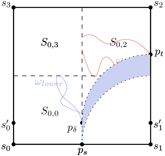
(a) The upper left $1\times 1$ subsquare $S_{0}$ of $P$.

(b) Visualization of Lemma 2.4.

Figure 1: Computing an optimal path $\omega$ through the square $S_{0}$.

Lemma 2.4.

For any $\delta>0$, $\omega$ has a subpath $p_{s}p_{\delta}$.

Proof 2.5.

We denote the part from $p_{s}$ to $S_{0,3}$ as the lower portion and from $S_{0,3}$ to $p_{t}$ as the upper portion of $\omega$, see Figure 1. Let $s_{1}^{\prime}=(1,\delta)$ and $\varepsilon=s_{1}s_{1}^{\prime}$. Segment $\varepsilon$ must be covered by $\omega$. We distinguish two cases; (i) $\varepsilon$ is covered by the lower portion of $\omega$ or (ii) $\varepsilon$ is covered by the upper portion of $\omega$. For case (i), let us assume that $\varepsilon$ is covered by the lower portion of $\omega$. When $\omega$ would enter $S_{0,1}$ it would also have to enter $S_{0,0}$ to cover the left side of $S_{0,0}$. It is clear that traversing the segment $p_{s}p_{\delta}$ of length $\delta$ is the best way to cover the lower portion of $S_{0,0},S_{0,1}$, as any other path would need additional segments in $x$-direction, see Figure 1(b). Any path that obeys case (ii) is suboptimal, as it has to cover $\varepsilon$ from within $S_{0,2}$, for a detour of at least $2\delta$.

Lemma 2.6.

The uniquely-shaped optimal Lawn Mowing path $\omega$ between two adjacent sides of $S_{0}$ has length $L_{S_{0}}\approx 1.309$ with $\omega=(p_{s},p_{\delta},q,p_{t})$ and

$$p_{s}=(\frac{1}{2},0)\quad p_{\delta}=(\frac{1}{2},\delta)\approx(\frac{1}{2},0.168)\quad q\approx(0.386,0.682)\quad p_{t}=(1,\frac{1}{2}+\delta)\approx(1,0.668).$$

Proof 2.7.

Let $s_{3}$ be the top left corner of $S_{0}$. We identify a shortest path for visiting one point $q$ on a circle $U$ with diameter $1$ centered in $s_{3}$ dependent on $\delta$, a necessary condition for a feasible path. Let $c=d(p_{\delta},q)+d(q,p_{t})$ be the distance from both points to $U$. Consider an ellipse $E$ with foci $p_{\delta},p_{t}$ that touches $U$ in a single point, see Figure 2(a). By definition, the intersection point $q$ minimizes the distance $c$. For $\delta\in[0,1]$ we want to find an intersection point between $E$ and $U$ that minimizes distance $c$. Let $p_{c}=(p_{c}^{x},p_{c}^{y})$ be the center point of $E$ and $d_{E}$ be the distance from the center point of $E$ and $a,b$ the major/minor axis.

$$p_{c}^{x}=\frac{3}{4}\quad p_{c}^{y}=\frac{1}{4}+\delta\quad d_{E}=d(p_{\delta},p_{c})=\frac{\sqrt{2}}{4}\quad a=\frac{1}{2}d_{E}\quad b=\sqrt{a^{2}-d_{E}^{2}}$$ (1)

The ellipse can now be defined with its center point $p_{c}$, the major/minor axis $a,b$ and the angle $\theta$, which is the angle between a line through $p_{\delta},p_{t}$ and the $x$-axis. We formulate the shortest path problem as a minimization problem while inserting Equation 1.

min $$c+\delta$$

s.t. $$x^{2}+(y-2)^{2}-\frac{1}{4} \leavevmode\nobreak\ =\leavevmode\nobreak\ 0$$

$$\dfrac{((x-p_{c}^{x})\cos(\theta)+(y-p_{c}^{y})\sin(\theta))^{2}}{a^{2}}+\dfrac{((x-p_{c}^{x})\sin(\theta)-(y-p_{c}^{y})\cos(\theta))^{2}}{b^{2}} \leavevmode\nobreak\ =\leavevmode\nobreak\ 1$$

$$\sqrt{(x-1)^{2}+(y-\delta)^{2}}+\sqrt{(x-2)^{2}+(y-1-\delta)^{2}}-c \leavevmode\nobreak\ =\leavevmode\nobreak\ 0$$

The objective minimizes the total length of the path $\omega$ with variables that encode the exact coordinates of $p_{\delta},q,p_{t}$. An intersection point of $E$ and $C$ with center $s_{3}=(0,1)$ is a solution to the first and second constraints, respectively. An exact optimization approach using Mathematica reveals that $\delta,q^{x},q^{y}$ can only be expressed as the first, third, and first roots of three irreducible high-degree polynomials $f_{\delta},f_{q^{x}},f_{q^{y}}$, see Equations 2, 3 and 4.

$$f_{\delta}(x)= $589\,824$x^{16}-$7\,077\,888$x^{15}+$41\,189\,376$x^{14}-$154\,386\,432$x^{13}+$$ (2)

$$$416\,788\,480$x^{12}-$857\,112\,576$x^{11}+$1\,383\,417\,856$x^{10}-$1\,779\,354\,624$x^{9}+$$

$$$1\,834\,437\,632$x^{8}-$1\,514\,108\,928$x^{7}+$992\,782\,336$x^{6}-$509\,312\,064$x^{5}+$$

$$$199\,354\,208$x^{4}-$57\,160\,752$x^{3}+$11\,200\,088$x^{2}-$1\,313\,928$x+$67\,417$$$

$$f_{q^{x}}(x)= $16\,777\,216$x^{16}-$29\,360\,128$x^{14}+$21\,757\,952$x^{12}-$8\,978\,432$x^{10}+$196\,608$x^{9}+$$ (3)

$$$2\,187\,264$x^{8}-$208\,896$x^{7}-$233\,472$x^{6}+$38\,400$x^{5}-$2432$x^{4}+$2304$x^{3}+$$

$$$1008$x^{2}-$648$x+$81$$$

$$f_{q^{y}}(x)= $16\,777\,216$x^{16}-$268\,435\,456$x^{15}+$2\,009\,071\,616$x^{14}-$9\,336\,520\,704$x^{13}+$$ (4)

$$$30\,152\,589\,312$x^{12}-$71\,751\,434\,240$x^{11}+$130\,119\,041\,024$x^{10}-$$

$$$183\,392\,632\,832$x^{9}+$202\,951\,155\,712$x^{8}-$176\,850\,272\,256$x^{7}+$$

$$$120\,867\,188\,736$x^{6}-$64\,057\,278\,976$x^{5}+$25\,783\,384\,192$x^{4}-$$

$$$7\,610\,732\,416$x^{3}+$1\,551\,687\,280$x^{2}-$194\,938\,464$x+$11\,350\,269$$$

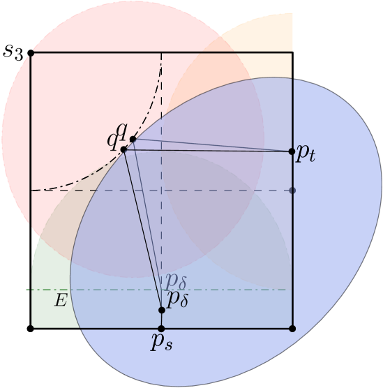
(a) Any $0\leq\delta\leq 1$ defines $p_{\delta},p_{t},q$ and ellipse $E$.

(b) The optimal path $\omega$ through $S_{0}$.

Figure 2: Visualizations for Lemma 2.6.

The value for $\delta\approx 0.167876$ defines the points $p_{\delta}$ and $p_{t}$. Together with the values for $q^{x},q^{y}$, we obtain the path above. The combined length of the path is $\delta+c\approx 1.308838224$. As $\omega$ contains a subpath that crosses the full height of $S_{0,0}$ and another subpath that crosses the full width of $S_{0,2}$, both quadrants are covered by $\omega$, see Figure 2(b). By construction, the bottom right quadrant is covered by the segment $p_{s}p_{\delta}$ and the point $p_{t}$. The top left quadrant is covered by $q$, because $S_{0,3}$ is fully contained in a disk with diameter $1$ centered in $q$. Therefore, $\omega$ is a feasible path between two adjacent edges of $S_{0}$ with a length of $L\approx 1.309$.

Lemma 2.8.

A square $P$ of side length $2$ has a uniquely-shaped optimal Lawn Mowing tour $T$ of length $L=4L_{S_{0}}$, where $L_{S_{0}}\approx 1.309$.

Proof 2.9.

We start by subdividing $P$ by its vertical and horizontal center line into four quadrants (squares) $S_{0},\dots,S_{3}$ with side length $1$. To cover the center point of each quadrant, a Lawn Mowing tour has to intersect it at least once. As $P$ is convex, $T$ cannot leave $P$ at any point. Finally, $T$ is symmetric with respect to the vertical and horizontal lines because otherwise, the quadrant subpaths could be replaced by the shortest one. By Lemma 2.6, there is a unique optimal Lawn Mowing path through each quadrant yielding an optimal tour of length $L=4L_{S_{0}}\approx 4\cdot 1.309\approx 5.235$, see Figure 3(a).

2.2 Galois Group of the Polynomial

Now we show that the coordinates of the optimal path $\omega$ can not be expressed by radicals. We employ a similar technique as Bajaj [7] for the generalized Weber problem. A field $K$ is said to be an extension (written as $K/\mathbb{Q}$) of $\mathbb{Q}$ if $K$ contains $\mathbb{Q}$. Given a polynomial $f(x)\in\mathbb{Q}[x]$, a finite extension $K$ of $\mathbb{Q}$ is a splitting field over $\mathbb{Q}$ for $f(x)$ if it can be factorized into linear polynomials $f(x)=(x-a_{1})\cdots(x-a_{k})\in K[x]$ but not over any proper subfield of $K$. Alternatively, $K$ is a splitting field of $f(x)$ of degree $n$ over $\mathbb{Q}$ if $K$ is a minimal extension of $\mathbb{Q}$ in which $f(x)$ has $n$ roots. Then the Galois group of the polynomial $f$ is defined as the Galois group of $K/\mathbb{Q}$. In principle, the Galois group is a certain permutation group of the roots of the polynomial. From the fundamental theorem of Galois theory, one can derive a condition for solvability by radicals of the roots of $f(x)$ in terms of algebraic properties of its Galois group. We state three additional theorems from Galois theory and Bajaj’s work. The proofs can be found in [7, 33].

Lemma 2.10 ([33]).

$f(x)\in\mathbb{Q}[x]$ is solvable by radicals over $\mathbb{Q}$ iff the Galois group over $\mathbb{Q}$ of $f(x)$, $Gal(f(x))$, is a solvable group.

Lemma 2.11 ([33]).

The symmetric group $S_{n}$ is not solvable for $n\geq 5$.

Lemma 2.12 ([7]).

If $n\equiv 0\mod 2$ and $n>2$ then the occurrence of an $(n-1)$-cycle, an $n$-cycle, and a permutation of type $2+(n-3)$ on factoring the polynomial $f(x)$ modulo primes that do not divide the discriminant of $f(x)$ establishes that $Gal(f(x))$ over $\mathbb{Q}$ is the symmetric group $S_{n}$.

Proof 2.13 (Proof of Theorem 2.1).

It suffices to show that $f_{\delta}$ is not solvable by the radicals as it describes the y-coordinates of two points in the solution. We provide three factorizations of $f_{\delta}$ modulo three primes that do not divide the discriminant $disc(f_{\delta}(x))$.

$$f_{\delta}(x)\equiv\; $12$(x^{16}+$11$x^{15}+$20$x^{14}+$20$x^{13}+$12$x^{12}+$15$x^{11}+$20$x^{10}+$22$x^{9}+$19$x^{8}+$2$x^{7}+$$

$$$18$x^{6}+$10$x^{5}+$12$x^{4}+$19$x^{3}+$16$x^{2}+$9$x+$8$)\mod 23$$

$$f_{\delta}(x)\equiv\; $21$(x+$44$)(x^{2}+$34$x+$39$)(x^{13}+$4$x^{12}+x^{11}+$41$x^{10}+$12$x^{9}+$21$x^{8}+$24$x^{7}+$$

$$$32$x^{5}+$22$x^{4}+$10$x^{3}+$24$x^{2}+$18$x+$13$)\mod 47$$

$$f_{\delta}(x)\equiv\; (x+$39$)(x^{15}+$8$x^{14}+$43$x^{13}+$23$x^{12}+$19$x^{11}+$38$x^{10}+$9$x^{9}+$6$x^{8}+$17$x^{7}+$$

$$$34$x^{6}+$46$x^{5}+$43$x^{4}+$27$x^{3}+$50$x^{2}+$56$x+$1$)\mod 59$$

For the good primes $p=23,47,$ and $59$, the degrees of the irreducible factors of $f_{\delta}(x)\mod p$ gives us an $16-cycle$, a $2+13$ permutation and a $15$-cycle, which is enough to show with Lemma 2.12 and $n=16$ that $Gal(f_{\delta})=S_{16}$. By Lemma 2.11, $S_{16}$ is not solvable; with Lemma 2.10, this proves the theorem.

3 Mowing Polyominoes

In the following, we analyze good tours for polyominoes, which naturally arise when a geometric (or geographic) region is mapped, resulting in axis-parallel edges and integer vertices. In the subsequent two sections, we describe the ensuing theoretical worst-case guarantees (Section 4) and the practical performance (Section 5).

3.1 Combinatorial Bounds

For a unit-square cutter, the LMP on polyominoes naturally turns into the TSP on the dual grid graph induced by pixel centers.

Lemma 3.1.

Let $N\geq 2$ be the area of a polyomino $P$ to be mowed with a unit-square cutter, and let $L$ be the minimum length of a Lawn Mowing tour. Then $L\geq N$. In the case of a unit-square cutter, $L=N$ iff the dual grid graph of $P$ has a Hamiltonian cycle.

This follows from Lemma 2 in the paper by Arkin et al. [4] (which argues that there is an optimal LMP tour for a polyomino whose vertices are pixel centers) and implies the NP-hardness of the LMP (Theorem 1 in [4]). In particular, they focused on grid graphs without a cut vertex, which is a node $v$ whose removal disconnects $G$: “If $G$ has a cut vertex $v$, then we can consider separately the approximation problem in each of the components obtained by removing $v$, and then splice the tours back together at the vertex $v$ to obtain a tour in the entire graph $G$. Thus, we concentrate on the case in which $G$ has no cut vertices.”

For a simply connected polyomino consisting of $N$ pixels, the corresponding grid graph $G$ does not have any holes, i.e., the complement of $G$ in the infinite integer lattice is connected. These allow a tight combinatorial bound on the tour length. If $G$ has no cut vertices, then a combinatorially bounded tour of $G$ exists, as noted by Arkin et al. [4] as follows.

Theorem 3.2 (Theorem 5 in [4]).

Let $G$ be a simple grid graph, having $N$ nodes at the centerpoints, $V$, of pixels within a simple rectilinear polygon, $R$, having $n$ (integer-coordinate) sides. Assume that $G$ has no cut vertices. Then, in time $O(n)$, one can find a representation of a tour, $T$, that visits all $N$ nodes of $G$, of length at most $\frac{6N-4}{5}$.

For polyominoes with holes, there is a slightly worse, but still relatively tight combinatorial bound of $\frac{53N}{40}=1.325N$ for the tour length, as follows.

Theorem 3.3 (Theorem 7 in [4]).

Let $G$ be a connected grid graph, having $N$ nodes at the centerpoints, $V$, of pixels within a (multiply connected) rectilinear polygon, $R$, having $n$ (integer-coordinate) sides. Assume that $G$ has no local cut vertices. Then, in time $O(n)$, one can find a representation of a tour, $T$, that visits all $N$ nodes of $G$, of length at most $1.325N$.

3.2 Mowing with a Disk

The natural lower bound of Lemma 3.1 still applies when mowing with a circular cutter, because any unit distance covered by the cutter can at most cover a unit area. However, meeting (or approximating) this bound is no longer possible by simply finding a Hamiltonian cycle (or a good tour) in the underlying grid graph, as a circular cutter may cover already mowed area or area outside of $P$ when dealing with pixel corners. Minimizing this effect ultimately leads to the algebraic analysis from the previous section.

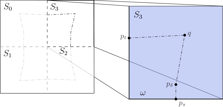
(a) Optimal Lawn Mowing tour for a $2\times 2$ square.

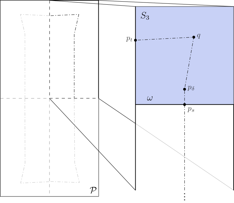
(b) Optimal Lawn Mowing tour for a rectangle.

Figure 3: Optimal Lawn Mowing tours for a square and a rectangle.

A starting point for further insights is illustrated in Figure 3: The optimal path from Lemma 2.6 with length $L_{S_{0}}$ can be used for rectangles with width $2$ and arbitrary height $h\geq 2$.

Corollary 3.4.

Any rectangle $P$ with width $2$ and height $h>2$ has a uniquely-shaped optimal Lawn Mowing tour $T$ of length $L=4L_{S_{0}}+2h-8$.

Extending this idea to more general polyominoes leads to realizing a tour of the dual grid with locally optimal “puzzle pieces”: a limited set of locally good trajectories that mow each visited pixel, which are merged at transition points on the pixel boundaries; see Figure 4(a). The construction of the puzzle pieces is done in Section 3.3.

(a) A pixel $S$ with transition points.

(b) A straight-line covering, with zero turn

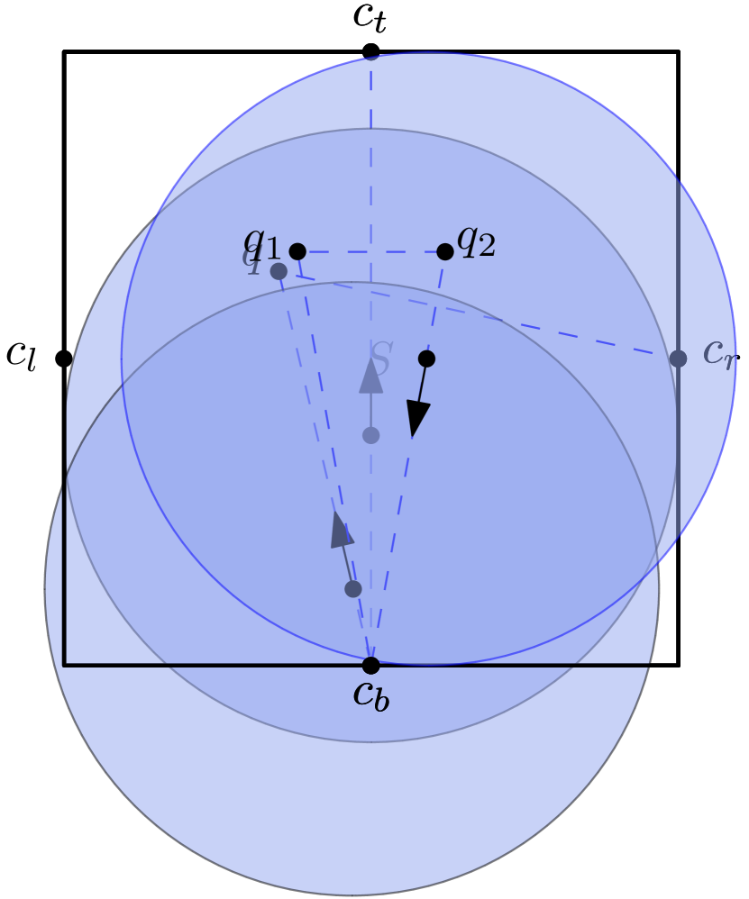
(c) A covering for a single, 90-degree turn

(d) A covering for a double, 180-degree U-turn

Figure 4: A pixel $S$ with three elementary covering trajectories.

3.3 Constructing Puzzle Pieces

In order to analyze locally good trajectories for mowing visited pixels, consider the four corners of a pixel with coordinates $(0,0),(1,0),(1,1),(0,1)$. We consider transition points $c_{b}=(1/2,0)$, $c_{r}=(1,1/2)$, $c_{t}=(1/2,1)$, and $c_{l}=(0,1/2)$ at the edge centers to ensure an overall connected trajectory, as shown in Figure 4(a). There are three combinatorially distinct ways for visiting a pixel, corresponding to Figures 4(b), 4(c) and 4(d). These are (i) a straight path, (ii) a simple turn, and (iii) a U-turn.

1. The straight path connects $c_{b}$ and $c_{t}$ and has length $L_{\omega}=1$, see Figure 4(b).

2. The simple turn connects $c_{b}$ and $c_{r}$. Solving a minimization problem similar to the one from the proof of Lemma 2.6 with a fixed $\delta=0$ yields a path $c_{b},q,c_{t}$ of length $L_{\omega}\approx 1.32566$ and $q=(\frac{1}{2\sqrt{2}},\frac{1}{4}(4-\sqrt{2}))$, see Figure 4(c).

3. The U-turn connects $c_{b}$ with itself while covering $S$ completely. An optimal solution must visit both circles of unit diameter centered at $(0,1),(1,1)$. Thus, we can formulate the following minimization problem

   min $$\sqrt{(x_{1}-\frac{1}{2})^{2}+y_{1}^{2}}+\sqrt{(x_{2}-\frac{1}{2})^{2}+y_{2}^{2}}+\sqrt{(x_{1}-x_{2})^{2}+(y_{1}-y_{2})^{2}\vphantom{\frac{1}{2}}}$$

   s.t. $$x_{1}^{2}+(y_{1}-1)^{2}-\frac{1}{4} =\leavevmode\nobreak\ 0$$

   $$(x_{2}-1)^{2}+(y_{2}-1)^{2}-\frac{1}{4} =\leavevmode\nobreak\ 0$$

   This yields an optimal solution $c_{b},q_{1},q_{2},c_{b}$ with $q_{1}\approx(0.383,0.678)$, $q_{2}\approx(0.617,0.678)$ and length $L_{\omega}\approx 1.611183$.

Note that we do not use the optimal path from Lemma 2.6, because it uses transition points that are slightly off center, $p_{t}\neq c_{r}$, with the imbalance canceled out between two adjacent simple turns. Thus, using central transition points incurs a small marginal cost when compared to an optimal trajectory ($1.32566$ vs. $1.309$, or about 1.2% longer for each simple turn), but it sidesteps the higher-order difficulties of combining longer off-center strips.

3.4 Building an Overall Tour

Making use of the puzzle pieces, we can now approach the LMP in three steps, as follows.

1. Find a cheap roundtrip on the dual grid graph.

2. Carry out the individual pixel transitions based on the above puzzle pieces as building blocks to ensure coverage of all pixels and thus a feasible tour.

3. Perform post-processing sensitive to the transition costs on the resulting tour to achieve further improvement.

In the following sections, we describe how the involved steps can be carried out either with an emphasis on worst-case runtime and worst-case performance guarantee (giving rise to theoretical approximation algorithms, as discussed in the following Section 4), or with the goal of good practical performance in reasonable time for a suite of benchmark instances (leading to the experimental study described in Section 5).

4 Theoretical Performance: Approximation

For constant-factor approximation, we start with a low-cost roundtrip in the dual grid graph (Step A), e.g., with the previous results of Arkin et al. [4]. Step B is realized using the puzzle pieces of Section 3.3 for a feasible tour, at a cost of $1+\tau:=1.32566$ for each 90-degree turn in the grid tour (corresponding to piece (ii)); note that the turn cost for a U-turn of $1.61118$ (corresponding to piece (iii)) does not exceed $1+2\tau$. By using combinatorial arguments for the post-processing Step C, we can prove that a limited number of covering turns (with an additional turn cost $\tau$) suffices for overall feasibility.

Theorem 4.1.

Let $P$ be a polyomino with $N>5$ pixels, and let $T$ be a tour of the dual grid graph of length $L$. Then we can find a feasible Lawn Mowing tour for a unit-diameter disk of length at most $L(1+\tau)$.

Proof 4.2.

Let $T$ be a tour of the dual grid graph; let $L$ be the length of $T$. $L$ is the total number of visits of individual pixels, inducing the following three categories of pixel visits.

1. $L_{0}$ “free” visits of pixels, in which no covering turn occurs, and no turn cost is incurred.

2. $L_{1}$ “one-turn” visits of pixels, in which one covering turn occurs, for a turn cost of $\tau$.

3. $L_{2}$ “U-turn” visits of pixels, in which a double covering turn occurs, for a turn cost of not more than $2\tau$.

Let $p_{i}$ be a pixel that is visited in step $i$ of the tour by a U-turn of $T$. Then $p_{i}$ is adjacent to a pixel $q=p_{i-1}=p_{i+1}$ that was left in step $i$ and entered in step $i+1$. Because no pixel visited by a U-turn needs to be visited more than once, as well as $N>5$, the pixel $q$ cannot only have neighbors that are visited by U-turns. Therefore, $q$ has a predecessor in the tour that is not a U-turn, (w.l.o.g., $p_{i-2}$); this visit from $p_{i-2}$ is either a one-turn visit with a covering turn, or a free visit. In either case, $q$ is already covered when visited from $p_{i}$, and we can simply follow the grid path at only the distance cost of 1.

As a consequence, each U-turn visit (incurring a cost not exceeding $2\tau$) can be uniquely mapped to a free visit of its successor (incurring no turn cost), and the overall cost for all covering turns does not exceed $L\tau$, for a total length of at most $L(1+\tau)$, as claimed.

For simple polyominoes without cut vertices, Theorem 3.2 provides a tour $T$ in the dual grid graph of length at most $\frac{6N-4}{5}$, implying the following.

Corollary 4.3.

Let $P$ be a simple polyomino with $n$ vertices and $N$ pixels, whose dual grid graph does not have any cut vertices. Then, in time $O(n)$, one can find a representation of a feasible Lawn Mowing trajectory $T$ for a unit-diameter disk of length at most $\frac{6N-4}{5}\tau$, which is within $1.5908$ of the optimum.

For polyominoes with holes, we can apply the same line of argument to a tour $T$ of the dual grid graph obtained from Theorem 3.3.

Corollary 4.4.

Let $P$ be a (not necessarily simple) polyomino with $n$ vertices and $N$ pixels, whose dual grid graph does not have any cut vertices. Then, in time $O(n)$, one can find a representation of a feasible Lawn Mowing trajectory $T$ for a unit-diameter disk of length at most $\frac{53N}{40}\tau$, which is within $1.7565$ of the optimum.

As the number of turns is of critical importance for the overall cost of a Lawn Mowing tour obtained from a tour of the dual grid graph, we can consider optimizing a linear combination of tour length and turn cost. Arkin et al. [2] gave a PTAS for this problem, as follows.

Theorem 4.5 (Theorem 5.17 in [2]).

Define the cost of a tour to be its length plus $C$ times the number of (90-degree) turns. For any fixed $\varepsilon>0$, there is a $(1+\varepsilon)$-approximation algorithm, with running time $2^{O(h)}N^{O(C)}$, for minimizing the cost of a tour for an integral orthogonal polygon $P$ with $h$ holes and $N$ pixels.

Combining tour length and turns allows providing more explicit bounds, as follows. Additional local considerations are possible, but these do not necessarily improve the worst-case bounds. Instead, they are employed heuristically in the practical section.

Theorem 4.6.

Let $P$ be a polyomino with $n$ vertices and $N$ pixels, and let $T$ be a tour of the dual grid graph of length $L$ and a total of $t$ (weighted) turns. Then there is a feasible Lawn Mowing tour of cost at most $L+t\tau$.

5 Practical Performance: Algorithm Engineering

5.1 Algorithmic Tools

Here we exploit the algorithmic approach of Section 3.4 for good practical performance for general polygonal regions, starting with a preprocessing step: For a given polygonal region $Q$, find a suitable polyomino $P$ that covers it.

We can then aim for practical minimization of tour length and turn cost for A (analogous to the theoretical Theorem 4.5), and use puzzle pieces in B for a feasible tour. In principle, we can approach A by considering an integer program (IP); however, solving this IP becomes too costly for larger instances, so we use a more scalable approach: (A) Find a good TSP solution on the dual grid graph; (B) insert puzzle pieces; (C) minimize the induced turn cost by Integer Programming and Large Neighborhood Search (LNS).

5.1.1 Choosing a Suitable Grid

Consider a non-degenerate polygonal region $Q$, and a minimal covering polyomino $P$ of cell size $\ell$. Without loss of generality, $Q$ contains only pixels with a point of $Q$ in their interior; furthermore, we can assume that both an $x$- and a $y$-coordinate of a grid point coincide with a coordinate of $Q$. This limits the number of relevant grid positions to a quadratic number of choices, from which one can choose the one with the smallest number of pixels contained in the resulting polygon $P$.

5.1.2 Minimizing Tour and Turn Cost

Finding a covering tour of minimum combined tour length and turn cost can be formulated as an IP. As the cost for each turn can be specified individually in this IP, we can also minimize the final tour length directly instead of just approximating it based on the number of turns. In principle, this IP can be solved with CPLEX [17] or Gurobi [29]; however, this fails when aiming for truly large instances. (Even without the length of the tour, the turn-cost problem is notoriously difficult [25].) Thus, we have pursued an alternative approach that starts with a cheap roundtrip on the dual grid graph in which we ignore the turn cost. We then use this IP as part of a Large Neighborhood Search (described in Section 5.1.4) to minimize the actual costs of this solution, and for computing lower bounds on the best possible solution based on puzzle pieces.

Formulating the Integer Program

To formulate the integer program, let $\widehat{uvw}$ with $uv,vw\in E_{H}$ be the puzzle piece covering the pixel $v$ and connecting $c_{uv}$ and $c_{vw}$, and $\overline{uvw}$ be the direct path between $c_{uv}$ and $c_{vw}$. We call these tour elements (covering and non-covering) tiles. We use the variables $x_{\widehat{uvw}}\in\mathbb{B},uv,vw\in E_{H}$ to denote which covering tile, i.e., puzzle piece, is used for $v\in V_{P}$ is in the tour. For simplicity, $x_{\widehat{uvw}}$ is also defined for $v\in V\setminus V_{P}$, but fixed to $0$. Analogously, we are using the variables $x_{\overline{uvw}}\in\mathbb{N}_{0},uv,vw\in E_{H}$ to denote how often which non-covering tiles, i.e., direct paths, for $v\in V$ are used in the tour. Because we may need to pass a pixel multiple times, this is an integer variable.

Finding the shortest set of cycles that cover all pixels $t\in V_{P}$ can be expressed as follows. Enforcing a single cycle, i.e., tour, is done later by some more complex constraints that need additional discussion.

$$\min \displaystyle\sum_{uv,vw\in E_{H}}||\overline{uvw}||\cdot x_{\overline{uvw}}+||\widehat{uvw}||\cdot x_{\widehat{uvw}}$$ (5)

s.t. $$\displaystyle\sum_{u,w\in N(v)}x_{\widehat{uvw}}=1 \forall v\in V_{P}$$ (6)

$$\begin{array}[]{l}\displaystyle 2\cdot(x_{\overline{wvw}}+x_{\widehat{wvw}})+\sum_{n\in N(v),n\not=w}(x_{\overline{nvw}}+x_{\widehat{nvw}})\\ =\displaystyle 2\cdot(x_{\overline{vwv}}+x_{\widehat{vwv}})+\sum_{n\in N(w),n\not=v}(x_{\overline{vwn}}+x_{\widehat{vwn}})\end{array} \forall vw\in E_{H}$$ (9)

$$x_{\widehat{vwv}}\in\mathbb{B},x_{\overline{vwv}}\in\mathbb{N}_{0} \forall uv,vw\in E_{H}$$ (10)

The objective function (5) minimizes the sum of lengths of the used tiles (the length of a tile is denoted by $||\cdot||$). Equation 6 enforces that every pixel $v\in V_{P}$ that intersects the polygon $P$ has one covering tile; $N(v)$ are the neighbors of $v$. Equation 9 ensures that every tile has a matching incident tile on each end, i.e., connecting all tiles yields feasible cycles.

Subtour Elimination

Next, we have to add constraints that enforce a single tour. A simple, but insufficient, constraint is similar to the classical subtour elimination constraint of the Dantzig-Fulkerson-Johnson formulation [18] for the Traveling Salesman Problem. For every non-empty subset $S\subset V,S\not=\emptyset,V\not\subset S,V\setminus S\not=\emptyset$ that contains a real part of $V_{P}$, there has to be some path leaving the set to connect to $V\setminus S$.

$$\sum_{uv,vw\in E_{H},v\in S,w\not\in S}x_{\overline{uvw}}+x_{\widehat{uvw}}\geq 1$$ (11)

Unfortunately, this is not sufficient as we can have cycles that cross but are not connected, e.g., for the tiles $\overline{uvw}$ and $\widehat{svt}$ with $\{u,w\}\cap\{s,t\}=\emptyset$. While they share the same pixel $v$ in the grid graph, the paths themselves do not have to intersect. We can also not expect them to be exchangeable as this may increase the objective. Let $O$ be a cycle of tiles that cover only a real subset of $V_{P}$, $E(O)$ denote the edges in the grid graph, and $\widehat{abc}\in O$ be a covering tile of $O$ with $b\in V(O)\cap V_{P}$. The following constraint now forces the path that covers $v$ to change and connect to exterior parts.

$$\sum_{u,w\in N(b),\widehat{ubw}\not\in O}x_{\widehat{ubw}}+\sum_{vw\in E(O),u\in N(v),\overline{uvw}\not\in O,\widehat{uvw}\not\in O}(x_{\overline{uvw}}+x_{\widehat{uvw}})\geq 1$$ (12)

This constraint is sufficient as it can be applied to any cycle that is covering only a subset of $V_{P}$, but generally less efficient.

5.1.3 Finding a Cheap Roundtrip and Ensure Coverage

We consider two different methods for computing different initial tours.

TSP${}_{\text{Small}}$:

Previous authors [12, 36, 41, 43] have suggested using a grid graph $H^{\prime}$ with smaller cell size $\ell=\frac{\sqrt{2}}{2}$ for covering $P$, or simply assumed square-shaped tools. This eliminates the need to consider any turn cost, as smaller pixels are covered when the cutter visits their centers. This yields TSP${}_{\text{Small}}$, which we use as a baseline. Because of the smaller grid size, this may result in double coverage when parallel unit strips suffice to cover the $P$, for a worst-case overhead of $\sqrt{2}-1$, or about $41.4\text{\,}\mathrm{\char 37\relax}$.

TSP${}_{\text{Cov}}$:

As described in the preceding Section 3, we can use a cheap tour for the grid graph $H$ with cell size $\ell=1$, and perform the puzzle piece modification. This combined solver is called TSP${}_{\text{Cov}}$. As shown in Section 4, we can limit the worst-case overhead for performing turns of TSP${}_{\text{Cov}}$ to $\tau=0.32566$ per length of the tour, or about $32.6\text{\,}\mathrm{\char 37\relax}$.

5.1.4 Improving the Tour

For a feasible tour from TSP${}_{\text{Cov}}$, we use an LNS-algorithm [40], which iteratively fixes a large part of the IP and only optimizes a small region of tiles; this yields TSP${}_{\text{Turn}}$. We select a random tile from the current tour and a fixed number of adjacent pixels. This yields a limited-size integer program, in which only the involved puzzle pieces are allowed to change. To escape local minima, we tune the size (and runtime) of the IP after each iteration based on the runtime of the previous iteration. In the end, we attempt to solve the IP on the complete instance, using the start solution from the LNS. This provides lower bounds on the best placement of puzzle pieces.

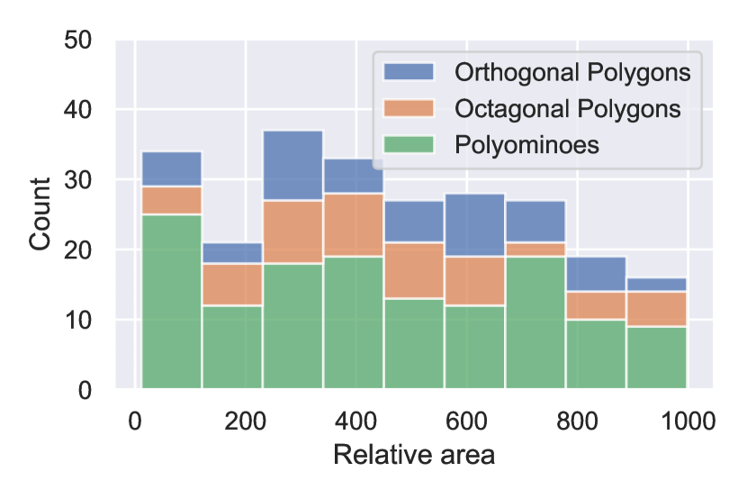
(a) Distribution of instances.

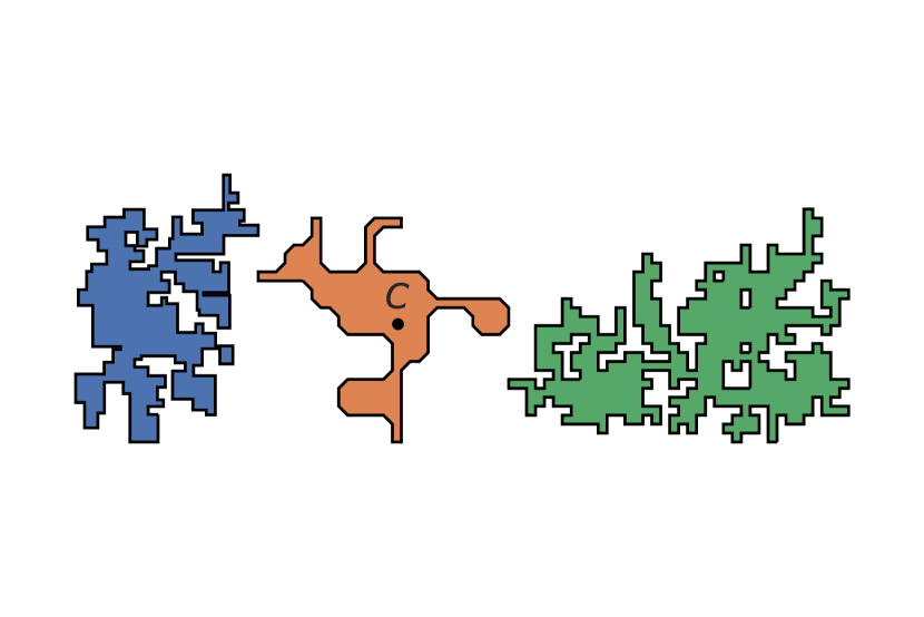
(b) Three instances with the cutter $C$.

Figure 5: Examples of the used polygons and their size distribution.

5.2 Experimental Setup

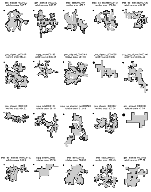
Figure 12: Examples of the used polygons. The black circles show the respective cutter size; the relative area denotes the ratio of convex hull area and cutter area.

Our practical implementation was tested on a workstation with an AMD Ryzen 7 5800X ($8\times$3.8\text{\,}\mathrm{GHz}$$) CPU and $128\text{\,}\mathrm{GB}$ of RAM. The code and data are publicly available. We used the srpg_iso, srpg_iso_aligned and srpg_octa instances and generated additional polyominoes with the open-source code from the Salzburg Database of Geometric Inputs [19]. See Figure 5 for the overall distribution and Figure 12 for examples. We considered polygons with up to $n=300$ vertices and a cutter with diameter 1. Overall, this resulted in $327$ instances. All experiments were carried out with a maximum runtime of $300\text{\,}\mathrm{s}$ for TSP, LNS and final IP computation. To solve the TSP efficiently, we used the python binding pyconcorde of the Concorde TSP Solver [42]. All components of TSP${}_{\text{Cov}}$ and TSP${}_{\text{Turn}}$ were implemented in Python 3.10 and used the IP solver Gurobi (v10.0) [29]. As in previous work [26] the relative area (ratio of convex hull area of $P$ and cutter area $A(C)$) is more significant for the difficulty of an instance than number of vertices of $P$.

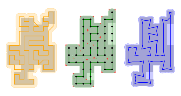
Figure 6: (Left) A TSP${}_{\text{Small}}$ tour yields a feasible but expensive LMP tour. (Middle) A TSP tour of the underlying dual grid graph, with uncovered patches shown in red. (Right) A feasible LMP tour after puzzle piece modification of the TSP tour.

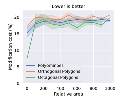
Figure 7: Modification cost over size and instance type. The modification induces a cost of around $19\text{\,}\mathrm{\char 37\relax}$ over all instance types and sizes. The plot shows the average modification cost and the $95\text{\,}\mathrm{\char 37\relax}$ confidence interval.

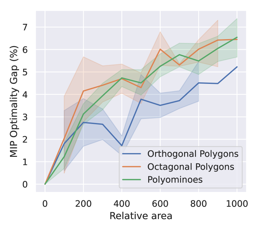
(a) Optimality gap of the IP.

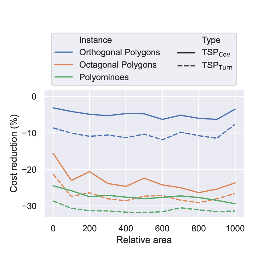
(b) Cost reduction.

Figure 8: (a) Remaining average optimality gaps for the integer program and the $95\text{\,}\mathrm{\char 37\relax}$ confidence interval. (b) Comparison of the average cost reduction for different approaches and polygon types.

5.3 Evaluation

We discuss our practical results along a number of research questions (RQ).

RQ1: How does TSP${}_{\text{Cov}}$ compare to TSP${}_{\text{Small}}$ in practice?

We compared the worst-case bound of $32.6\text{\,}\mathrm{\char 37\relax}$ for TSP${}_{\text{Cov}}$ to the actual performance, using the total cost of TSP${}_{\text{Small}}$ as a baseline. See Figure 6 for an example and Figure 7 for the average relative modification cost. This shows not more than an additional $19\text{\,}\mathrm{\char 37\relax}$ cost, with only small variation over size and type. Figure 8(b) shows that the practical average reduction from TSP${}_{\text{Small}}$ is independent from the size of the polygon, but differs strongly for the different instance classes; we save $\approx$27\text{\,}\mathrm{\char 37\relax}$$ for polyominoes, $\approx$24\text{\,}\mathrm{\char 37\relax}$$ for octagonal polygons, and $\approx$5\text{\,}\mathrm{\char 37\relax}$$ for orthogonal polygons.

RQ2: How good are the solutions achieved by TSP${}_{\text{Turn}}$?

For the considered large instances, provably optimal solutions for the turn-cost minimizing IP are hard to find, so we considered the remaining optimality gap in the IP. Figure 8(a) shows that gaps remain below $7\text{\,}\mathrm{\char 37\relax}$ even for large instances, and below $5\text{\,}\mathrm{\char 37\relax}$ on average for medium-sized instances.

We also compared the tours from TSP${}_{\text{Cov}}$ with the cheapest tours obtained by TSP${}_{\text{Turn}}$ and TSP${}_{\text{Small}}$. As shown in Figure 8(b), on average we obtain $\approx$5\text{\,}\mathrm{\char 37\relax}$$ shorter tours when compared to the TSP${}_{\text{Cov}}$ tours, independent of instance size and type. For orthogonal polygons, this doubles the cost reduction.

RQ3: How far are we from the geometric area lower bound?

A remaining gap between TSP${}_{\text{Turn}}$ and the area bound may result from two sources, both from (i) the quality of the upper bound (and thus TSP${}_{\text{Turn}}$) and (ii) the quality of the area lower bound, for the following reasons. (i) The optimal LMP tour is not restricted to the grid graph $H$, so there may be cheaper tours than what we obtain from TSP${}_{\text{Turn}}$. (ii) The simple area bound (corresponding to Lemma 3.1) is relatively weak, so it is conceivable that a serious gap to this lower bound remains.

Overall, the combination of both effects remains limited, as can be seen from Figure 9 (showing the ratio of TSP${}_{\text{Turn}}$ value and area bound): For the octagonal polygons and polyominoes, we are on average at most $50\text{\,}\mathrm{\char 37\relax}$ above the area bound. For orthogonal polygons, the relative gap is on average below $80\text{\,}\mathrm{\char 37\relax}$.

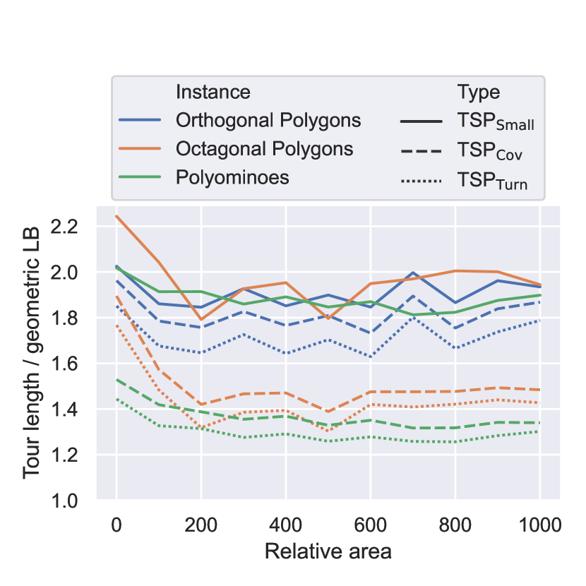
(a) Tour length compared to the area bound.

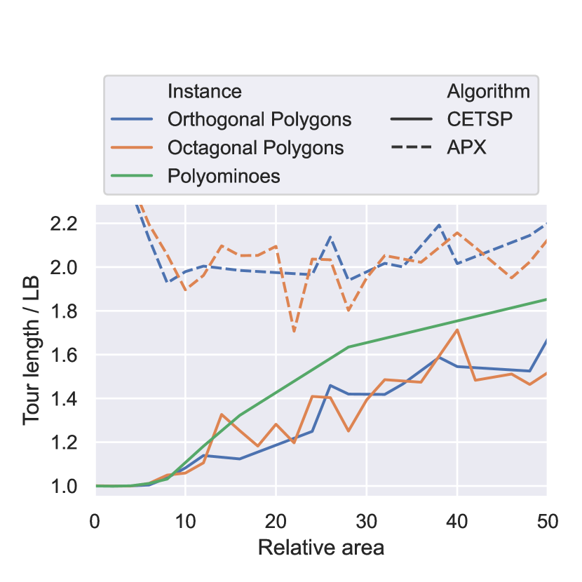
(b) Solution quality of [26].

Figure 9: (a) Tour length compared to the (weaker) area lower bound in terms of the average ratio. For octagonal polygons and polyominoes, we can get below $50\text{\,}\mathrm{\char 37\relax}$ on average. (b) Comparable results for the average solution quality of [26] based on a (stronger) CETSP bound; here APX denotes the performance of the approximation algorithm by [4]. Note the considerably larger relative area in comparison to [26].

RQ4: How do our solutions compare to previous practical work?

As shown before, our results are already considerably better than work based on TSP${}_{\text{Small}}$. A comparison to the previous best practical results by Fekete et al. [26] (whose instances were used as a subset of our benchmarks) is shown in Figure 9; plotted are the ratios between the achieved solution values and the respective lower bounds. Fekete et al. [26] employ a more sophisticated lower bound based on an evaluation of a series of Close-Enough TSP (CETSP) instances. The authors pointed out that the lower bound computation becomes very expensive even for instances with relative area smaller than $50$, see Figures $11$ and $12$ in [26]. Because we evaluate much larger instances, our ratios only use the relatively straightforward area bound. As a consequence, the denominators of these ratios favor the evaluation for [26], which are shown in Figure 9(b); see Figures 10(a) and 10(b) for a comparison on a relatively small example that was also shown in [26]. In addition, we were able to achieve results for instances with a relative area 20 times larger than [26].

Despite these additional challenges (of weaker bounds and larger instance sizes), our results compare favorably to the ones reported by [26]. The main reason lies in our structurally simpler approach that still yields good results when the complex evaluation of the CETSP from [26] reaches computational limitations. As can be seen from a comparison of computed trajectories for the visual example (Figures 10(c) and 10(d)), this is also reflected in simpler trajectories obtained from TSP${}_{\text{Turn}}$.

(a) Area (LB): $36.25$

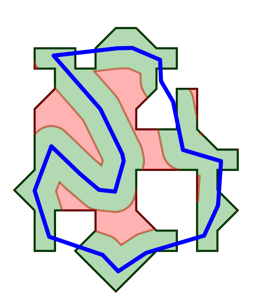
(b) LB: $40.94$ [26]

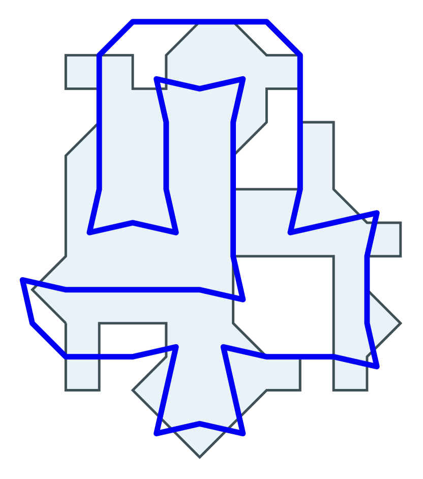
(c) TSP${}_{\text{Turn}}$ (UB): $66.71$

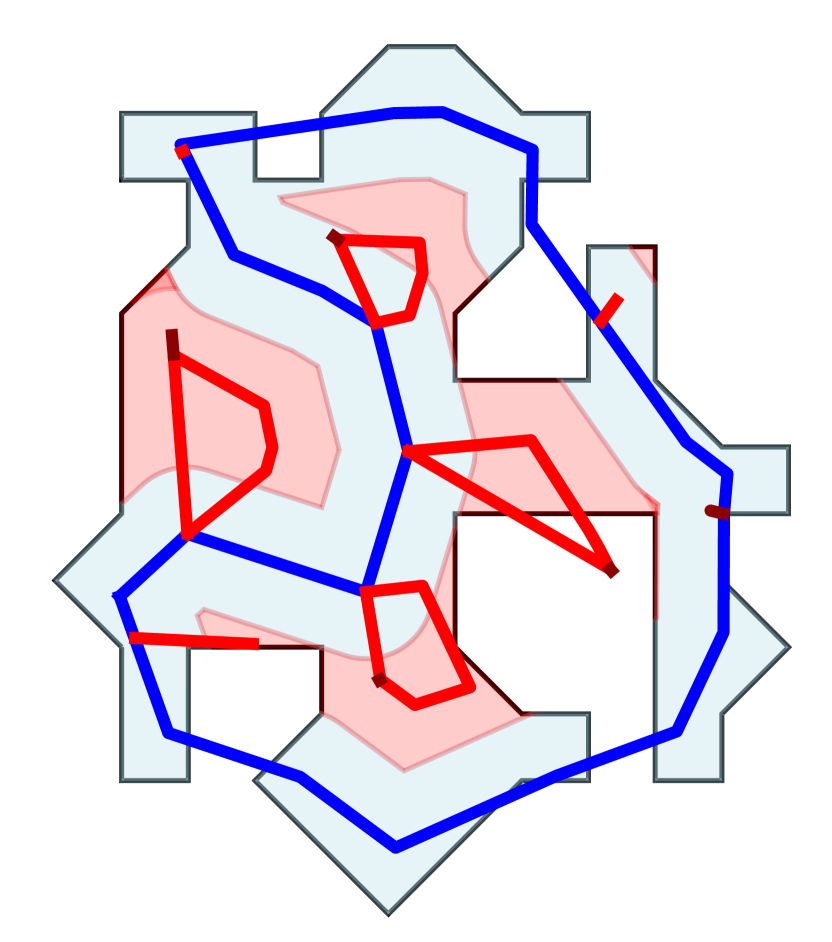
(d) UB: $68.16$ [26]

Figure 10: Comparison of TSP${}_{\text{Turn}}$ with lower and upper bounds from Fekete et al. [26].

6 Conclusion

We have presented new insights for the Lawn Mowing Problem, starting with an algebraic analysis of the structure of optimal trajectories. As a consequence, we can pinpoint a particular source of the perceived overall difficulty of the problem, and prove that constructing optimal tours necessarily involves operations that go beyond simple geometric means; we can also use these insights to come up with better construction methods for tours, both on the theoretical and the practical side, with minimizing overall turn cost playing a crucial role.

Our results also clear the way for a number of important followup questions. Is it possible to improve our approach for polyominoes? As discussed in the text, considering higher-order connectivity between turns and using slightly off-center, axis-parallel strips appears to be a relatively easy way for (albeit marginal) improvement. It may very well be that this ultimately leads to optimal tours for polyominoes; however, final success on this fundamental challenge will require another breakthrough in establishing lower bounds, as neither the polygon area (which may incur a gap from the optimal value, similar to the number of vertices in a grid graph does from a TSP solution) nor the Close-Enough TSP bound for a finite set of witness points may suffice to certify optimality. Given that an optimal tour may also involve portions that are not axis-parallel, it will also require further algebraic analysis of turns that are not multiples of 90 degrees.

For the Lawn Mowing Problem on general regions (which may not even have to be connected), our hardness result hints at further difficulties. It is quite conceivable that the general LMP is not just algebraically hard, but even $\exists\mathbb{R}$-complete. Even in that case, we believe that further engineering of the tile-based mowing of polyominoes (with attention to turn cost) and Close-Enough TSP may be the most helpful tools for further systematic improvement.

Appendix A Source Code for Algebraic Verification of Lemma 2.6

Source Code 1: Mathematica source code for the calculating the optimal values for $p_{\delta},q,p_{t}$

⬇

1r = 1 / 2;

2xPos[delta_] := 3/2* r

3yPos[delta_] := 1/2 * (r + delta*r + delta*r)

4

5Dist[x_, y_, z_, v_] := Sqrt[(x - z)^2 + (y - v)^2]

6Angle[x_, y_, z_, v_] := VectorAngle[{x - z, y - v}, {1, 0}]

7

8Theta[x_, y_, delta_] := Pi - Angle[r, delta*r, 2 r, r + delta*r]

9f[delta_] := Dist[xPos[delta], yPos[delta], r, r*delta]

10a[x_, y_, delta_] := 1/2 * (Dist[x, y, r, delta*r] + Dist[x, y, 2 r, r + delta*r])

11b[x_, y_, delta_] := Sqrt[a[x, y, delta]^2 - f[delta]^2]

12

13ellipseEquation[x_, y_, delta_] := ((x - xPos[delta])* Cos[Theta[x, y, delta]] + (y - yPos[delta])* Sin[Theta[x, y, delta]])^2/ a[x, y, delta]^2 + ((x - xPos[delta])* Sin[Theta[x, y, delta]] - (y - yPos[delta])* Cos[Theta[x, y, delta]])^2/b[x, y, delta]^2

14

15distanceToQ[x_, y_, delta_] := Dist[x, y, r, delta*r] + Dist[x, y, 2 r, r + delta*r]

16distanceToCircleCenter[x_, y_] := x^2 + (y - 2 *r)^2

17

18result =

19 Minimize[{c + delta*r,

20 distanceToCircleCenter[x, y] == r^2 &&

21 ellipseEquation[x, y, delta] == 1 &&

22 distanceToQ[x, y, delta] - c == 0 && 0 <= delta <= 1 &&

23 0 <= x <= r && r <= y <= 2 r && c > 0}, {x, y, c, delta}];

24

25yReduce = RootReduce[y /. Last@result];

26xReduce = RootReduce[x /. Last@result];

27deltaReduce = RootReduce[delta /. Last@result];

Appendix B Additional Figures

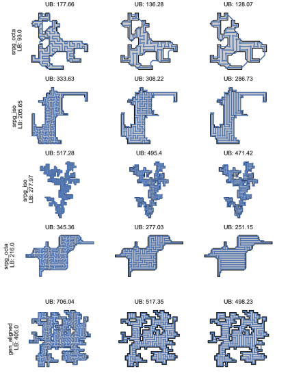
Figure 11: Examples of different solutions. Left column is the TSP${}_{\text{Small}}$ solver which operates on a $\sqrt{2}/2$ grid. The middle column shows solutions to TSP${}_{\text{Cov}}$ which operates on a larger grid. The right column shows TSP${}_{\text{Turn}}$ solutions which modify and improve the TSP${}_{\text{Cov}}$ solution by minimizing the number of turns.

References

- [1] David L. Applegate, Robert E. Bixby, Vašek Chvátal, and William J. Cook. The Traveling Salesman Problem: A Computational Study. Princeton Series in Applied Mathematics. Princeton University Press, 2007. doi:10.1016/j.orl.2007.06.002.
- [2] Esther M. Arkin, Michael A. Bender, Erik D. Demaine, Sándor P. Fekete, Joseph S. B. Mitchell, and Saurabh Sethia. Optimal covering tours with turn costs. SIAM Journal on Computing, 35(3):531–566, 2005. doi:10.1137/S0097539703434267.
- [3] Esther M. Arkin, Sándor P. Fekete, and Joseph S. B. Mitchell. The lawnmower problem. In Canadian Conference on Computational Geometry (CCCG), pages 461–466, 1993. URL: https://cglab.ca/~cccg/proceedings/1993/Paper79.pdf.
- [4] Esther M. Arkin, Sándor P. Fekete, and Joseph S. B. Mitchell. Approximation algorithms for lawn mowing and milling. Computational Geometry, 17:25–50, 2000. doi:10.1016/S0925-7721(00)00015-8.
- [5] Esther M. Arkin, Martin Held, and Christopher L. Smith. Optimization problems related to zigzag pocket machining. Algorithmica, 26(2):197–236, 2000. doi:10.1007/s004539910010.
- [6] Rik Bähnemann, Nicholas Lawrance, Jen Jen Chung, Michael Pantic, Roland Siegwart, and Juan Nieto. Revisiting Boustrophedon coverage path planning as a generalized traveling salesman problem. In Field and Service Robotics, pages 277–290, 2021. doi:10.1007/978-981-15-9460-1_20.
- [7] Chanderjit Bajaj. The algebraic degree of geometric optimization problems. Discrete & Computational Geometry, 3(2):177–191, 1988. doi:10.1007/BF02187906.
- [8] Michael J. Bannister, William E. Devanny, David Eppstein, and Michael T. Goodrich. The galois complexity of graph drawing: Why numerical solutions are ubiquitous for force-directed, spectral, and circle packing drawings. Journal of Graph Algorithms and Applications, 19(2):619–656, 2015. doi:10.7155/jgaa.00349.
- [9] Aaron T. Becker, Mustapha Debboun, Sándor P. Fekete, Dominik Krupke, and An Nguyen. Zapping zika with a mosquito-managing drone: Computing optimal flight patterns with minimum turn cost. In Symposium on Computational Geometry (SoCG), pages 62:1–62:5, 2017. Video at https://www.youtube.com/watch?v=SFyOMDgdNao. doi:10.4230/LIPIcs.SoCG.2017.62.
- [10] Károly Bezdek. Körök optimális fedései (Optimal Covering of Circles). PhD thesis, Eötvös Lorand University, 1979.
- [11] Károly Bezdek. Über einige optimale Konfigurationen von Kreisen. Ann. Univ. Sci. Budapest Rolando Eötvös Sect. Math, 27:143–151, 1984.
- [12] Richard Bormann, Joshua Hampp, and Martin Hägele. New brooms sweep clean - an autonomous robotic cleaning assistant for professional office cleaning. In IEEE International Conference on Robotics and Automation (ICRA), pages 4470–4477, 2015. doi:10.1109/ICRA.2015.7139818.
- [13] Tauã M. Cabreira, Lisane B. Brisolara, and Paulo R. Ferreira Jr. Survey on coverage path planning with unmanned aerial vehicles. Drones, 3(1):4, 2019. doi:10.3390/drones3010004.
- [14] Jean-Lou De Carufel, Carsten Grimm, Anil Maheshwari, Megan Owen, and Michiel H. M. Smid. A note on the unsolvability of the weighted region shortest path problem. Computational Geometry, 47(7):724–727, 2014. doi:10.1016/j.comgeo.2014.02.004.
- [15] Howie Choset. Coverage for robotics–a survey of recent results. Annals of Mathematics and Artificial Intelligence, 31(1):113–126, 2001. doi:10.1023/A:1016639210559.
- [16] Howie Choset and Philippe Pignon. Coverage path planning: The Boustrophedon cellular decomposition. In Field and Service Robotics, pages 203–209, 1998. doi:10.1007/978-1-4471-1273-0_32.
- [17] International Business Machines Corporation. IBM ILOG CPLEX Optimization Studio, 2023.
- [18] George Dantzig, Ray Fulkerson, and Selmer Johnson. Solution of a large-scale traveling-salesman problem. Journal of the Operations Research Society of America, 2(4):393–410, 1954. doi:10.1287/opre.2.4.393.
- [19] Günther Eder, Martin Held, Steinþór Jasonarson, Philipp Mayer, and Peter Palfrader. Salzburg database of polygonal data: Polygons and their generators. Data in Brief, 31:105984, 2020. doi:10.1016/j.dib.2020.105984.
- [20] Gershon Elber and Myung-Soo Kim. Offsets, sweeps and Minkowski sums. Computer-Aided Design, 31(3), 1999. doi:10.1016/S0010-4485(99)00012-3.
- [21] Brendan Englot and Franz Hover. Sampling-based coverage path planning for inspection of complex structures. In International Conference on Automated Planning and Scheduling (ICAPS), pages 29–37, 2012. URL: http://www.aaai.org/ocs/index.php/ICAPS/ICAPS12/paper/view/4728.
- [22] Gábor Fejes Tóth. Thinnest covering of a circle by eight, nine, or ten congruent circles. Combinatorial and Computational Geometry, 52:361–376, 2005. URL: http://library.msri.org/books/Book52/files/18fejes.pdf.
- [23] Sándor P. Fekete, Utkarsh Gupta, Phillip Keldenich, Christian Scheffer, and Sahil Shah. Worst-case optimal covering of rectangles by disks. In Symposium on Computational Geometry (SoCG), pages 42:1–42:23, 2020. doi:10.4230/LIPIcs.SoCG.2020.42.
- [24] Sándor P. Fekete, Phillip Keldenich, and Christian Scheffer. Covering rectangles by disks: The video. In Symposium on Computational Geometry (SoCG), pages 71:1–75:5, 2020. https://www.youtube.com/watch?v=Cwn9ZimX2XE. doi:10.4230/LIPIcs.SoCG.2020.75.
- [25] Sándor P. Fekete and Dominik Krupke. Practical methods for computing large covering tours and cycle covers with turn cost. In Algorithm Engineering and Experiments (ALENEX), pages 186–198, 2019. doi:10.1137/1.9781611975499.15.
- [26] Sándor P. Fekete, Dominik Krupke, Michael Perk, Christian Rieck, and Christian Scheffer. A closer cut: Computing near-optimal lawn mowing tours. In Symposium on Algorithm Engineering and Experiments (ALENEX), pages 1–14, 2023. doi:10.1137/1.9781611977561.ch1.
- [27] Erich Friedman. Circles covering squares web page. https://erich-friedman.github.io/packing/circovsqu, 2014. Online, accessed January 10, 2023.
- [28] Enric Galceran and Marc Carreras. A survey on coverage path planning for robotics. Robotics and Autonomous Systems, 61(12):1258–1276, 2013. doi:10.1016/j.robot.2013.09.004.
- [29] Gurobi Optimization, LLC. Gurobi Optimizer Reference Manual, 2023.
- [30] Martin Held. On the Computational Geometry of Pocket Machining, volume 500 of LNCS. Springer, 1991. doi:10.1007/3-540-54103-9.
- [31] Martin Held, Gábor Lukács, and László Andor. Pocket machining based on contour-parallel tool paths generated by means of proximity maps. Computer-Aided Design, 26(3):189–203, 1994. doi:10.1016/0010-4485(94)90042-6.
- [32] Aladár Heppes and Hans Melissen. Covering a rectangle with equal circles. Periodica Mathematica Hungarica, 34(1-2):65–81, 1997. doi:10.1023/A:1004224507766.
- [33] Israel N. Herstein. Topics in algebra. John Wiley & Sons, 1991.
- [34] Katharin R. Jensen-Nau, Tucker Hermans, and Kam K. Leang. Near-optimal area-coverage path planning of energy-constrained aerial robots with application in autonomous environmental monitoring. IEEE Transactions on Automation Science and Engineering, 18(3):1453–1468, 2021. doi:10.1109/TASE.2020.3016276.
- [35] Johannes B. M. Melissen and Peter C. Schuur. Covering a rectangle with six and seven circles. Discrete Applied Mathematics, 99(1-3):149–156, 2000. doi:10.1016/S0166-218X(99)00130-4.
- [36] Ghulam Murtaza, Salil S. Kanhere, and Sanjay K. Jha. Priority-based coverage path planning for aerial wireless sensor networks. In IEEE International Conference on Intelligent Sensors, Sensor Networks and Information Processing (IPSN), pages 219–224, 2013. doi:10.1109/ISSNIP.2013.6529792.
- [37] Eric H. Neville. On the solution of numerical functional equations. Proceedings of the London Mathematical Society, 2(1):308–326, 1915. doi:10.1112/plms/s2_14.1.308.
- [38] David Nistér, Richard I. Hartley, and Henrik Stewénius. Using galois theory to prove structure from motion algorithms are optimal. In IEEE Computer Society Conference on Computer Vision and Pattern Recognition (CVPR), 2007. doi:10.1109/CVPR.2007.383089.
- [39] Timo Oksanen and Arto Visala. Coverage path planning algorithms for agricultural field machines. Journal of Field Robotics, 26(8):651–668, 2009. doi:10.1002/rob.20300.
- [40] David Pisinger and Stefan Ropke. Large neighborhood search. Handbook of metaheuristics, pages 99–127, 2019. doi:10.1007/978-3-319-91086-4_4.
- [41] Gokarna Sharma, Ayan Dutta, and Jong-Hoon Kim. Optimal online coverage path planning with energy constraints. In International Conference on Autonomous Agents and MultiAgent Systems (AAMAS), pages 1189–1197, 2019. URL: https://dl.acm.org/doi/10.5555/3306127.3331820.
- [42] Solver, Concorde TSP. Concorde TSP Solver, 2023. URL: https://www.math.uwaterloo.ca/tsp/concorde.html.
- [43] Xiaoming Zheng, Sven Koenig, David Kempe, and Sonal Jain. Multirobot forest coverage for weighted and unweighted terrain. IEEE Transactions on Robotics, 26(6):1018–1031, 2010. doi:10.1109/TRO.2010.2072271.